Kinematic design and analysis of a novel overconstraint walking mechanism

Abstract

Walking mechanisms offer advantages over wheels or tracks for locomotion but often require complex designs. This paper presents the kinematic design and analysis of a novel overconstrained spatial a single degree-of-freedom leg mechanism for walking robots. The mechanism is generated by combining spherical four-bar linkages into two interconnecting loops, resulting in an overconstrained design with compact scalability. Kinematic analysis is applied using recurrent unit vector methods. Dimensional synthesis is performed using the Firefly optimization algorithm to achieve a near-straight trajectory during the stance phase for efficient walking. Constraints for mobility, singularity avoidance, and transmission angle are also implemented. The optimized design solution is manufactured using 3D printing and experimentally tested. Results verify the kinematic properties including near-straight-line motion during stance. The velocity profile shows low perpendicular vibrations. Advantages of the mechanism include compact scalability allowing variable stride lengths, smooth motion from overconstraint, and simplicity of a single actuator. The proposed overconstrained topology provides an effective option for the leg design of walking robots and mechanisms.

1. Introduction

Walking mechanisms offer several advantages over conventional modes of locomotion such as wheels or tracks. These advantages include reduced vibration through the discrete contact of endpoints, the ability to traverse multiple terrains with minimal contact area, controllable vehicle height, increased traction, climbing abilities, and obstacle negotiation. Inspired by the walking motion of humans, insects, and animals, walking mechanisms have been developed and used in various applications such as rehabilitation, search and rescue, military, and entertainment. As such, they have gained significant attention in the field of robotics, where they offer a versatile and adaptable means of locomotion.

A considerable amount of literature has been published on walking mechanisms. One of the most popular walking mechanisms is presented in Jansen’s work [1]. Jansen’s work has been a reference for many researchers. Ghassaei [2] has designed and analyzed the crank-based leg mechanism using Jansen’s mechanism as a reference walking paths required for walking are compared. As a result of the optimizations made, the aimed mechanism was designed and produced. Kim et al. [3] used an algorithm to design the leg length of a legged walking robot based on the Theo Jansen mechanism, utilizing kinematic analysis, and demonstrated the validity of the method through simulation results. Nansai et al. [4] analyzed the dynamics of a four-legged Theo Jansen mechanism robot. They used the projection method while making an analysis. Bhavsar et al. [5] have performed kinematic and dynamic analyses of the eight-legged Theo Jansen mechanism. In addition to these analyses, they have shown the changes in energy consumption because of the changes made. Daniel et al. [6] designed a new walking mechanism with reference to Theo Jansen’s mechanism. In their design, they aimed to optimize the step length and energy consumption of the Theo Jansen mechanism.

There are many researchers who have worked on the optimization of single degree-of-freedom (DoF) leg mechanisms. Klann [7] designed a single DoF mechanism to represent animal gait. Kim et al. [8] designed a Klann’s mechanism that can travel both in water and on land. James et al. [9] designed a single DoF bi-pedal walking robot. In the tests, they mentioned that it was more inefficient at low speeds than at high speeds. Anthony et al. [10] designed a Klann’s mechanism with two DoF controlled by two motors and capable of traveling both on land and in water. Gong et al. [11] designed a four-legged climbing robot with two DoF and handling capability. Selvi et al. [12] used the firefly algorithm to optimize a planar linkage for the minimum number of links for walking. In Selvi et al. [13], a single-loop 6R overconstrained leg mechanism is generated for walking using the firefly algorithm. Desai et al. [14] presented a planar Peaucellier-Lipkin type with eight walking mechanism links and optimized the dimensions for a straight line using genetic algorithms. In the work of Tsai et al. [15], a single DoF leg mechanism with only six bars is proposed and optimized where they get a symmetric curvy path for the leg tip without straight lines. Deb and Tiwari [16] solved the optimization problem simultaneously using evolutionary multi-objective optimization for the exact mechanism.

Furthermore, many researchers in the literature have studied walking mechanisms. Fedorov and Birglen [17] created an obstacle-avoiding-legged robot using Hoeckens-pantograph leg architecture and a passive trigger. Kamidi et al. [18] designed a six-link mechanism with a single DoF. Four of the designed mechanisms were positioned on a platform to create a fast-walking robot. Ottaviano et al. [19] designed a low-cost single DoF biped machine for a rickshaw robot, validated through kinematic analysis and experimental tests, demonstrating its feasibility in various operating conditions. Geonea et al. [20] optimized the design solution to achieve proper motion of the mechanism and foot trajectory, formulating kinematic equations for the proposed leg mechanism; they simulated the walking activity while considering ground and foot contact as well as joint friction, obtaining joint reaction forces and contact forces. Al-Araidah et al. [21] presented a nine-bar single DoF path generator that simulates the shape and motion of a human leg, featuring design specifications for leg slenderness and the shape of the walking gait, and validated the mechanism’s usability through simulation, demonstrating the feasibility of a single DoF closed-loop mechanical linkage for biped human walking. Wu and Yao [22] developed and tested a walking leg that can transform its topological structure by shifting the joint type. Li et al. [23] analyzed the walking of dogs and derived a walking path. They designed a walking mechanism with reference to this path. Wang et al. [24] designed a mechanism with reference to the joints of kangaroos and performed kinematic analyses of the designed mechanism. Gonzalez et al. [25] designed a legged or hybrid robot with three DoF. The designed robot has lateral sliding, straight-line drawing, and obstacle-jumping capabilities. Böttcher [26] talked about legged and wheeled locomotion in his seminar. In the walking mechanisms chapter, he talked about the foot configurations required for single, double, four, and six-legged mechanisms to be able to walk. He explained the position of the legs with respect to the center of gravity of the robot. Zhonghua and Yingmiao [27] proposed a four-legged robot designed for climbing stairs, utilizing a single DoF planar eight-link mechanism; they derived the motion equation of the leg under different assembly conditions to obtain the foot endpoint trajectory and validated the kinematics analysis. Al-Shammari et al. [28] designed a hexapod robot for use in different land conditions. Gu et al. [29] built a four-legged robot with an overconstrained link with a single DoF. This robot is characterized by being omnidirectional. Hao et al. [30] performed a foot kinematics simulation for the designed single-leg walking mechanism, verifying that the robot’s design meets the requirements of motion law and stationarity. Kong [31] has analyzed the kinematics of a six-joint single-loop overconstrained spatial mechanism. Lu et al. [32] designed a four-legged robot with two DoF. In their work, they analyzed the kinematic analysis and walking path of the robot. Lu et al. [33] designed a hybrid robot with wheels and legs. These legs are activated in case the robot climbs stairs or jumps obstacles. Considering this situation, they analyzed the gait of the foot mechanism. Saha [34] built a sweeping robot using Hoeken and Pantograph mechanisms. Sweeping motion represents a walking path. Chen et al. [35] designed an eight-bar walking mechanism. They highlighted that the eight-bar walking mechanism is superior to the four-link and six-link mechanisms and can better meet the required movement needs. Zang et al. [36] proposed a global scale analysis method for the kinematic performance of mechanisms, using singular theory, geometric topology, and group theory. The method is applied to a six-bar agile bionic leg mechanism (ABLM) and is validated through virtual prototype simulation, while its application to a four-bar linkage is compared with the Grashof’s criterion. A comprehensive framework for the innovative design and analysis of ABLM is introduced. Sheba et al. [37] designed a novel reconfigurable Klann mechanism that can produce various useful gait cycles. They solved the position analysis problem using a bilateration method and aimed to generate useful gaits by changing the linkage configurations. The study identified and analyzed five gait patterns, validating the approach and enhancing the original design’s capabilities. Li et al. [38] designed a robot walker based on a new single DoF six-bar leg mechanism, providing rectilinear, non-rotating foot movement. The walker is statically stable and requires only two actuators for walking on a flat surface. They used curvature theory to design a four-bar linkage with a flat-sided coupler curve and added a translating link for rectilinear movement. When these studies are analyzed, it is seen that the proposed mechanisms have advantages such as being easy to produce because they are planar, some have high obstacle-jumping capacity, and some have less fluctuation during walking. On the other hand, limitations include the large number of joints and links, the shorter path compared to the body length, less oscillation during walking compared to some mechanisms, and the enlargement of the whole mechanism when we want to enlarge the walking path.

This paper proposes a spatial two-loop single DoF overconstrained leg mechanism for a walking machine. Overconstrained mechanism generation from linkage configuration is explained as devoted to the walking mechanism. Then kinematic solution is described using recurrent unit vectors for the proposed mechanism. The scalability of the mechanism and its benefits are defined, and different possible configurations of the mechanism are discussed. Objective functions and constraints are detailed for the optimization design process. The firefly algorithm is used for optimization, and linkage parameters are calculated for the desired objective. The kinematic properties of the solution design are analyzed in terms of position velocity and acceleration results. The actuator torque values and properties for the designed overconstrained mechanisms are compared with other a single DoF leg mechanism. Test setup was prepared to obtain an experimental comparison with dynamic simulation to velocity and walking path.

2. Topology design for overconstrained leg mechanism proposal

Scalability for a mechanism can be described as a property where the construction parameters of a given manipulator can be altered to achieve scaled end effector motion. This property can be classified into two groups: complex and compact. Complex scalability forces to alter all the construction parameters of the manipulator, while compact scalability allows reaching the desired scaled motion by only altering a minimal number of construction parameters. Some overconstrained mechanisms are, by nature, compact scalable. Therefore, this work is aimed at an overconstrained compact scalable walking mechanism with a single DoF.

The design problem is continued by using the mechanism from the study of Selvi et al. [13] as a starting point. While this mechanism is also compact scalable, it couldn’t a create straight line. For this reason, we decided to use a double-loop mechanism to increase the number of parameters for synthesis.

The design of the mechanism consists of four main stages. The endpoint of the newly designed mechanism is aimed to be operated in a planar plane. To achieve this, as shown in Fig. 1a, two revolute joints are initially utilized in the creation of the mechanism, allowing it to execute the desired movements in the plane.

Table I. Unit vector calculation sequence for mechanism in Fig. 2.

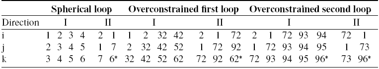
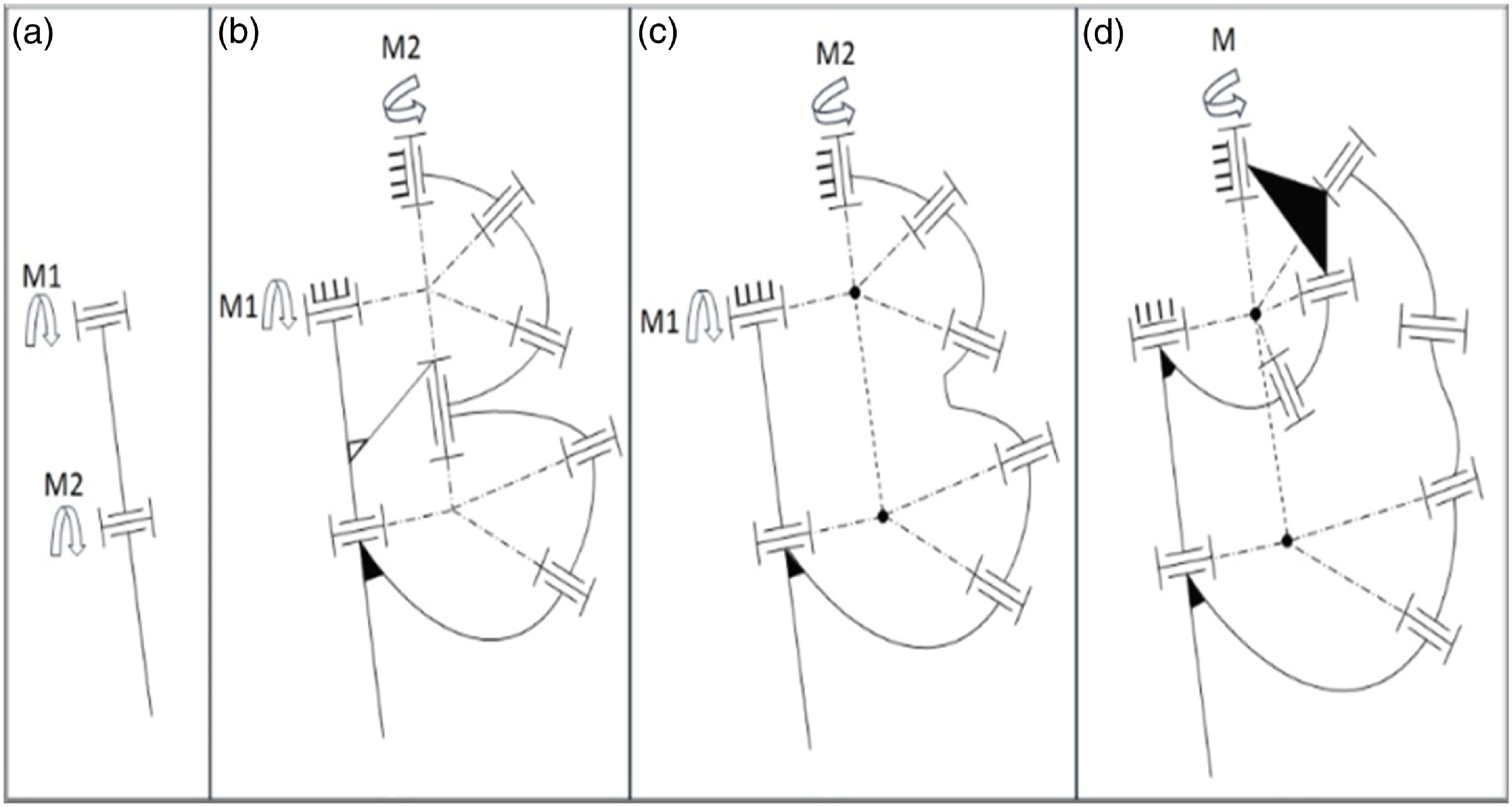
Figure 1. Progress stages of the overconstrained leg mechanism.

In the second stage, the aim is to transfer the motion from the second joint to the body. To accomplish this, two spherical four-bar mechanisms are incorporated into the mechanism initially presented in Fig. 1a, as seen in Fig. 1b. A common revolute joint is employed by intersecting one of the existing revolute joints. Additionally, the components labeled M1 and M2 in Fig. 1a are raised, and these joints are designated as fixed points by attaching motors to them.

In the third stage, with the help of an overconstrained loop structure, the joint that is commonly used is removed to reduce the number of joints and links, as depicted in Fig. 1c. Consequently, a double spherical bar linkage with λ=5 is derived. However, even in this configuration, two motors are still in use, resulting in two DoF.

In the final step, the motors are consolidated into a single location, as shown in Fig. 1d. Two additional revolute joints are added at the position of the relocated motor, creating a spherical four-bar mechanism. As a result, a mechanism with a single DoF driven by a solitary motor is defined.

DoF of the mechanism is verified using Alizade’s [39] formula for multi-loop mechanisms with variable subspace numbers in the form:

(2a) \begin{equation}DoF=\sum _{i=1}^{n}f_{i}-\sum _{i=1}^{2}{\unicode[Arial]{x03BB}} _{i}\end{equation}

where λ is the space or subspace number and f_i is the i^th joint DoF. Therefore, the mechanism has two independent loops: the first loop is in a spherical subspace with λ = 3, and the second loop is overconstrained with one general constraint loop with λ = 5. There are nine revolute joints in the mechanism so that the DoF of the mechanism is calculated as 9 – (5 + 3) = 1.

3. Kinematics analysis

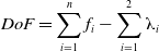
The present work involves a kinematic analysis of the mechanism with constant crank rotation, as well as the use of foot position equations to optimize the path of walking mechanisms. Recurrent unit vector algebra is employed to determine the equations for kinematic calculations. The unit vectors, referred to as "s_i," which describe the joints and links of the mechanism in Fig. 2, are calculated using recurrent unit vector algebra method [40]. The sequential use of recurrent unit vectors for each loop is shown in Table I.

Figure 2. Representation of the mechanism with unit vectors attached to joints and links axes.

To determine the unit vectors for the joints and links of the mechanism depicted in Fig. 2 and to use them in the analysis, Eq. (3a) is utilized. The unit vectors S ₁ and S ₂ are initially attached to the ground link and are placed on the z and x coordinates respectively, as described in Eq. (3b).

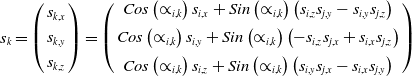(3a) \begin{equation}\boldsymbol{s}_{\boldsymbol{k}}=\left(\begin{array}{c} s_{k,x}\\[3pt] s_{k,y}\\[3pt] s_{k,z} \end{array}\right)=\left(\begin{array}{c} Cos\left(\propto _{i,k}\right)s_{i,x}+Sin\left(\propto _{i,k}\right)\left(s_{i,z}s_{j,y}-s_{i,y}s_{j,z}\right)\\[5pt] Cos\left(\propto _{i,k}\right)s_{i,y}+Sin\left(\propto _{i,k}\right)\left(-s_{i,z}s_{j,x}+s_{i,x}s_{j,z}\right)\\[5pt] Cos\left(\propto _{i,k}\right)s_{i,z}+Sin\left(\propto _{i,k}\right)\left(s_{i,y}s_{j,x}-s_{i,x}s_{j,y}\right) \end{array}\right)\end{equation}

Where ${\unicode[Arial]{x03B1}} _{\mathrm{i},\mathrm{k}}$ is the angle between i^th and the k^th unit vector

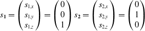(3b) \begin{equation}\boldsymbol{s}_{\mathbf{1}}=\left(\begin{array}{c} s_{1,x}\\ s_{1,y}\\ s_{1,z} \end{array}\right)=\left(\begin{array}{c} 0\\ 0\\ 1 \end{array}\right)\boldsymbol{s}_{\mathbf{2}}=\left(\begin{array}{c} s_{2,x}\\ s_{2,y}\\ s_{2,z} \end{array}\right)=\left(\begin{array}{c} 0\\ 1\\ 0 \end{array}\right)\end{equation}

For the analysis of the first spherical loop, Eq. (3b) is employed to perform recurrent calculations of the other unit vectors, as outlined in Table I. The unit vectors s_i , s_j , and s_k , where the indices i, j, and k denote specific joints or links within the mechanism, are systematically determined through this iterative process. This approach allows for the refinement of each vector’s orientation at each step in the calculation.

In this context, s₆ is calculated from both directions of the loop, with the notation s_6* indicating that the vector is derived from direction II. This reflects the recurrent nature of the calculations, which build on previous iterations to ensure accurate alignment. By structuring the calculations in this manner, as detailed in Table I, the method effectively supports the kinematic analysis, ensuring that each unit vector contributes meaningfully to the overall understanding of the mechanism’s motion. The indices i, j, and k for the unit vectors correspond to different components of the mechanism, helping to organize the calculations and track how each vector evolves throughout the analysis.

In particular referring to the solution two spherical loops in Table I, eliminating ${\unicode[Arial]{x03B1}} _{3,5}$ from equality of $s_{6}={s_{6}}^{\mathrm{*}}$ and solving for ${\unicode[Arial]{x03B1}} _{2,7}$ gives

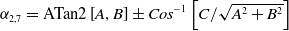(3c) \begin{equation}\alpha _{2,7}=\text{ATan}2\left[A,B\right]\pm Cos^{-1}\left[C/\sqrt{A^{2}+B^{2}}\right]\end{equation}

where

\begin{equation*} A=\mathrm{Cos}\left[\alpha _{1,3}\right]\mathrm{Sin}\left[\alpha _{1,8}\right]\mathrm{Sin}\left[\alpha _{2,4}\right] \end{equation*}

\begin{equation*} B=-\mathrm{Cos}\left[\alpha _{2,4}\right]\mathrm{Sin}\left[\alpha _{1,8}\right] \end{equation*}

\begin{equation*} C=-\left(\mathrm{Cos}\left[\alpha _{4,6}\right]-\mathrm{Cos}\left[\alpha _{1,8}\right]\mathrm{Sin}\left[\alpha _{1,3}\right]\mathrm{Sin}\left[\alpha _{2,4}\right]\right) \end{equation*}

Then using equality of $s_{6}={s_{6}}^{\mathrm{*}}, \alpha _{3,5}$ can be found as

(3d) \begin{equation}\alpha _{3,5}=ATan2[Cos\left(\alpha _{3,5}\right),Sin\left(\alpha _{3,5}\right)]\end{equation}

where

\begin{align*} \mathrm{Sin}\left[\alpha _{3,5}\right]&=\mathrm{Cos}\left[\alpha _{1,8}\right]\mathrm{Csc}\left[\alpha _{4,6}\right]\mathrm{Sec}\left[\alpha _{1,3}\right]\\&+\left(-\mathrm{Cot}\left[\alpha _{4,6}\right]\mathrm{Csc}\left[\alpha _{2,4}\right]+\mathrm{Cot}\left[\alpha _{2,4}\right]\mathrm{Csc}\left[\alpha _{4,6}\right]\mathrm{Sin}\left[\alpha _{1,8}\right]\mathrm{Sin}\left[\alpha _{2,7}\right]\right)\mathrm{Tan}\left[\alpha _{1,3}\right] \end{align*}

\begin{equation*} \mathrm{Cos}\left[\alpha _{3,5}\right]=\mathrm{Cot}\left[\alpha _{2,4}\right]\mathrm{Cot}\left[\alpha _{4,6}\right]-\mathrm{Csc}\left[\alpha _{2,4}\right]\mathrm{Csc}\left[\alpha _{4,6}\right]\mathrm{Sin}\left[\alpha _{1,8}\right]\mathrm{Sin}\left[\alpha _{2,7}\right] \end{equation*}

To increase the number of variables for optimization, constants ф_n are introduced as initial angles of respective joints. For example, ф₁ and ф₂ are added to joint angles $\alpha _{1,3}$ and $\alpha _{2,7}$ , and $\alpha _{1,32}$ and $\alpha _{2,72}$ are introduced, respectively, which also will be used in the optimization as construction parameters.

\begin{equation*} \alpha _{1,32}=\alpha _{1,3}+{\unicode[Arial]{x03D5}} _{1};\,\alpha _{2,72}=\alpha _{2,7}+{\unicode[Arial]{x03D5}} _{2}; \end{equation*}

Eliminating $\alpha _{32,52}$ from equality of $s_{62}={s_{62}}^{\mathrm{*}}$ and solving for $\alpha _{1,92}$ gives

(3e) \begin{equation}\alpha _{1,92}=\text{ATan}2\left[D,E\right]\pm Cos^{-1}\left[F/\sqrt{D^{2}+E^{2}}\right]\end{equation}

where

\begin{equation*} D=\left(-\mathrm{Cos}\left[\alpha _{1,32}\right]\mathrm{Cos}\left[\alpha _{2,72}\right]\mathrm{Sin}\left[\alpha _{2,42}\right]+\mathrm{Cos}\left[\alpha _{2,42}\right]\mathrm{Sin}\left[\alpha _{2,72}\right]\right)\mathrm{Sin}\left[\alpha _{72,82}\right] \end{equation*}

\begin{equation*} E=-\mathrm{Sin}\left[\alpha _{1,32}\right]\mathrm{Sin}\left[\alpha _{2,42}\right]\mathrm{Sin}\left[\alpha _{72,82}\right] \end{equation*}

\begin{equation*} F=-\left(\mathrm{Cos}\left[\alpha _{42,62}\right]-\mathrm{Cos}\left[\alpha _{72,82}\right]\left(\mathrm{Cos}\left[\alpha _{2,42}\right]\mathrm{Cos}\left[\alpha _{2,72}\right]+\mathrm{Cos}\left[\alpha _{1,32}\right]\mathrm{Sin}\left[\alpha _{2,42}\right]\mathrm{Sin}\left[\alpha _{2,72}\right]\right)\right) \end{equation*}

Similar to spherical loop, $\alpha _{32,52}$ can be found from equality of $s_{62}={s_{62}}^{\mathrm{*}}$ from the first imaginary spherical loop of the overconstrained loop:

(3f) \begin{equation}\alpha _{32,52}=ATan2[Sin\left(\alpha _{32,52}\right),Cos\left(\alpha _{32,52}\right)]\end{equation}

where

\begin{align*} \mathrm{Sin}\left[\alpha _{32,52}\right]&=-\mathrm{Csc}\left[\alpha _{42,62}\right]\left(\mathrm{Cos}\left[\alpha _{72,82}\right]\mathrm{Sin}\left[\alpha _{1,32}\right]\mathrm{Sin}\left[\alpha _{2,72}\right]\right.\\ & \left.+\left(\mathrm{Cos}\left[\alpha _{1,92}\right]\mathrm{Cos}\left[\alpha _{2,72}\right]\mathrm{Sin}\left[\alpha _{1,32}\right]-\mathrm{Cos}\left[\alpha _{1,32}\right]\mathrm{Sin}\left[\alpha _{1,92}\right]\right)\mathrm{Sin}\left[\alpha _{72,82}\right]\right) \end{align*}

\begin{align*} \mathrm{Cos}\left[\alpha _{32,52}\right]&=\mathrm{Csc}\left[\alpha _{42,62}\right]\mathrm{Sec}\left[\alpha _{2,42}\right]\mathrm{Sin}\left[\alpha _{1,32}\right]\mathrm{Sin}\left[\alpha _{1,92}\right]\mathrm{Sin}\left[\alpha _{72,82}\right]\\ & +\mathrm{Cos}\left[\alpha _{1,32}\right]\mathrm{Csc}\left[\alpha _{42,62}\right]\mathrm{Sec}\left[\alpha _{2,42}\right]\left(\mathrm{Cos}\left[\alpha _{72,82}\right]\mathrm{Sin}\left[\alpha _{2,72}\right] \right.\\ & \left.+\mathrm{Cos}\left[\alpha _{1,92}\right]\mathrm{Cos}\left[\alpha _{2,72}\right]\mathrm{Sin}\left[\alpha _{72,82}\right]\right)-\mathrm{Cot}\left[\alpha _{42,62}\right]\mathrm{Tan}\left[\alpha _{2,42}\right] \end{align*}

$\alpha _{1,93}$ is introduced adding another synthesis parameter ${\unicode[Arial]{x03D5}} _{3}$ to $\alpha _{1,92}$ :

(3g) \begin{equation}\alpha _{1,93}={\unicode[Arial]{x03D5}} _{3}+\alpha _{1,92};\end{equation}

Eliminating $\alpha _{93,95}$ from equality of $s_{96}={s_{96}}^{\mathrm{*}}$ and solving for $\alpha _{72,73}$ gives

(3h) \begin{equation}\alpha _{72,73}=\text{ATan}2\left[G,H\right]\pm Cos^{-1}\left[J/\sqrt{G^{2}+H^{2}}\right]\end{equation}

where

\begin{equation*} G=-\mathrm{Cos}\left[\alpha _{72,94}\right]\mathrm{Sin}\left[\alpha _{1,74}\right] \end{equation*}

\begin{equation*} H=\mathrm{Cos}\left[\alpha _{1,93}\right]\mathrm{Sin}\left[\alpha _{1,74}\right]\mathrm{Sin}\left[\alpha _{72,94}\right] \end{equation*}

\begin{equation*} J=-\left(\mathrm{Cos}\left[\alpha _{94,96}\right]-\mathrm{Cos}\left[\alpha _{1,74}\right]\mathrm{Sin}\left[\alpha _{1,93}\right]\mathrm{Sin}\left[\alpha _{72,94}\right]\right) \end{equation*}

Similar to spherical loop, $\alpha _{93,95}$ can be found from equality of $s_{96}={s_{96}}^{\mathrm{*}}$ from the second imaginary spherical loop of the overconstrained loop:

(3i) \begin{equation}\alpha _{93,95}=ATan2[Sin\left(\alpha _{93,95}\right),Cos\left(\alpha _{93,95}\right)]\end{equation}

where

\begin{align*} \mathrm{Sin}\left[\alpha _{93,95}\right]&=\left(\mathrm{Csc}\left[\alpha _{94,96}\right]\left(\mathrm{Sin}\left[\alpha _{1,93}\right]\left(\mathrm{Cos}\left[\alpha _{2,72}+\alpha _{72,73}\right]\mathrm{Cos}\left[\alpha _{72,94}\right]\mathrm{Sin}\left[\alpha _{1,74}\right]\right.\right.\right.\\&\left.\left.\left.+\mathrm{Cos}\left[\alpha _{94,96}\right]\mathrm{Sin}\left[\alpha _{2,72}\right]\right)+\mathrm{Cos}\left[\alpha _{1,74}\right]\left(\mathrm{Cos}\left[\alpha _{1,93}\right]\mathrm{Cos}\left[\alpha _{2,72}\right]\mathrm{Cos}\left[\alpha _{72,94}\right]\right.\right.\right.\\&\left.\left.\left.-\mathrm{Sin}\left[\alpha _{2,72}\right]\mathrm{Sin}\left[\alpha _{72,94}\right]\right)\right)\right)\left(\mathrm{Cos}\left[{\alpha _{2,72}}\right]\mathrm{Cos}\left[{\alpha _{72,94}}\right]-\mathrm{Cos}\left[{\alpha _{1,93}}\right]\mathrm{Sin}\left[{\alpha _{2,72}}\right]\mathrm{Sin}\left[{\alpha _{72,94}}\right]\right)^{-1} \end{align*}

\begin{align*} \mathrm{Cos}\left[\alpha _{93,95}\right]&=\left(\mathrm{Csc}\left[\alpha _{94,96}\right]\mathrm{Sec}\left[\alpha _{72,94}\right]\left(-\mathrm{Cos}\left[\alpha _{2,72}+\alpha _{72,73}\right]\mathrm{Csc}\left[\alpha _{2,72}\right]\mathrm{Sin}\left[\alpha _{1,74}\right]\right.\right.\\&\left.\left.+\mathrm{Cos}\left[\alpha _{1,74}\right]\mathrm{Cot}\left[\alpha _{2,72}\right]\mathrm{Tan}\left[\alpha _{1,93}\right]\right)\right.\\&\left.-\mathrm{Cot}\left[\alpha _{94,96}\right]\left(1+\mathrm{Cot}\left[\alpha _{2,72}\right]\mathrm{Sec}\left[\alpha _{1,93}\right]\mathrm{Tan}\left[\alpha _{72,94}\right]\right)\right)\left(\mathrm{Cot}\left[{\alpha _{2,72}}\right]\mathrm{Sec}\left[{\alpha _{1,93}}\right]-\mathrm{Tan}\left[{\alpha _{72,94}}\right]\right)^{-1} \end{align*}

$\alpha _{72,75}$ is introduced by adding another synthesis parameter ${\unicode[Arial]{x03D5}} _{4}$ to $\alpha _{72,73}$ :

(3j) \begin{equation}\alpha _{72,75}=\alpha _{72,73}+{\unicode[Arial]{x03D5}} _{4};\end{equation}

$\alpha _{2,72}and \alpha _{72,75}$ are used to find the position change of the path point P(P_x P_y) as shown in equation:

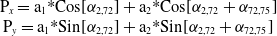(3k) \begin{equation}\begin{array}{c} \mathrm{P}_{x}=\mathrm{a}_{1}\text{*Cos}[\alpha _{2,72}]+\mathrm{a}_{2}\text{*Cos}[\alpha _{2,72}+\alpha _{72,75}]\\ \mathrm{P}_{y}=\mathrm{a}_{1}\text{*Sin}[\alpha _{2,72}]+\mathrm{a}_{2}\text{*Sin}[\alpha _{2,72}+\alpha _{72,75}] \end{array}\end{equation}

P_x and P_y define the path of the extremity of the leg concerning input α_1,3, which will be used later in the optimization design of the link lengths for a desired strider length and step height. If we define a₁ = k₁ * L and a₂ = k₂* L, Eq. (3k) shows that the path is independent of the radius of the spherical links; thus, they can independently be scaled without affecting the kinematic characteristic of the mechanism.

4. Leg trajectory for walking mechanisms

The locus of the P path consists of four segments as shown in Fig. 3. These are drive, lift, return, and lower. During the driving phase the foot is in contact with the ground and carries the weight of the body. In the lifting phase, the leg is lifted to overcome any obstacle and is crossed in the turning phase. The height of the obstacle it can pass is called the step height. Finally, the foot touches the ground again.

The kinematic analysis resulted in eight different path combinations. The combinations consist of multiple solutions in Eqs. (3c), (3f), and (3h). The walking paths obtained from alternative results are shown with respect to the general coordinate system (green lines) in Table II. In the table, + and - in the configuration section represent the sign at the beginning of the equations. Each of the lines in the Trial Result section is defined as 100 mm. Changes in walking were compared using stride to height of the step ratio and stride to leg height ratio. The larger both of these ratios, the greater the length of the distance taken by the mechanism when it completes one cycle and the height of the obstacle it can skip. Table II shows that in some of the walking paths, the height of the step ratio is large, but the stride to leg height ratio is small. Therefore, from the data in Table II, a combination with (+++) is selected for construction.

Table II. Alternative path solutions from Eqs. (3c), (3e), and (3h).

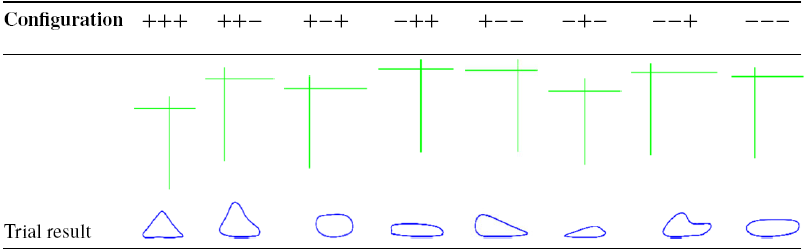
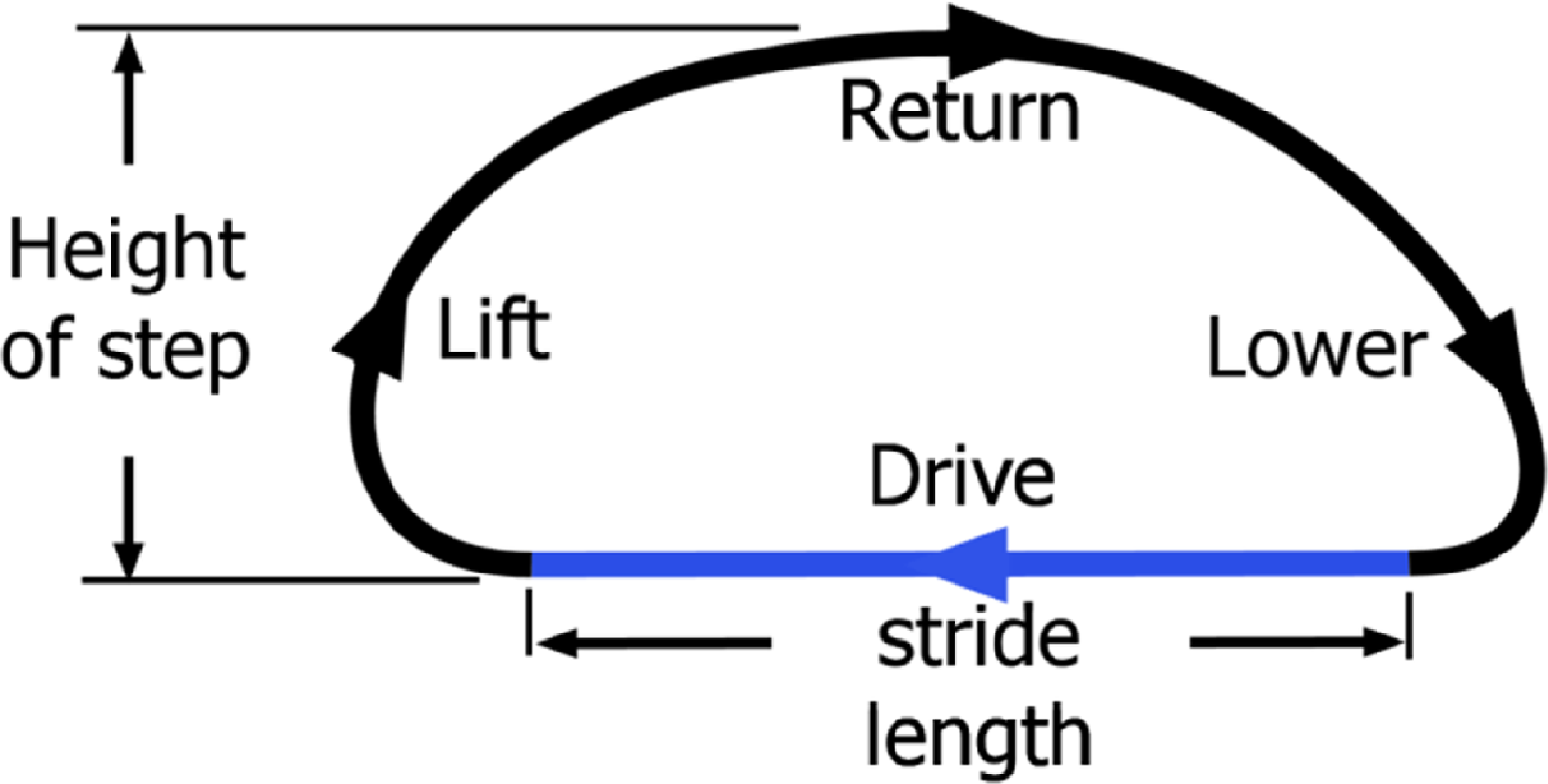
Figure 3. Locus of the leg mechanism during walking.

5. Optimization design using firefly algorithm

One of the optimization methods that generates a high-precision solution with a nonlinear approach to the nonlinear constrained problem is firefly algorithm [41]. It is a metaheuristic method using agents called fireflies that attract each other due to their lightness, which is related to the value of the objective function.

5.1. Objective function

The objective function for optimizing the mechanism’s path is formulated to minimize position errors while achieving desired path characteristics, including a specific stride length (s) of 86 mm. It considers the Euclidean distance of points along the straight part of the path to reduce y-direction variations. The function incorporates three key elements: the difference between the maximum y-value and the desired maximum y-value of −131 mm, the absolute difference between the maximum and minimum x-values compared to the desired x-range of 86 mm, and the cumulative difference between each of the 120 of the 360 path points’ y-values and the desired minimum y-value of −164 mm. These differences are weighted by a factor of 10 to balance their influence on the optimization. The firefly algorithm uses maximization; therefore, an inverted version of the error function is used. As the error approaches zero, the optimization result (objective function value) approaches a small value, which reflects minimized errors and indicates a near-optimal solution. The objective function is expressed mathematically as follows:

Maximize

(5a) \begin{equation}f\left(x\right)=1/\left\{1+10\left(y_{max}-y_{\textit{desired}}\right)+10\left(Abs\left[x_{max}-x_{min}\right]-s\right)+\sum _{i=1}^{120}\left(y_{i}-y_{\textit{desired}}\right)\right\}\end{equation}

By considering the following constraint conditions.

5.2. Constraint functions

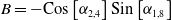
Three constraints that consider Grashof’s Law, transmission angle, and the range of design variables are imposed on the mechanism for full mobility.

5.2.1. Grashof’s criterion

In order to ensure the continuous rotation in the spherical four-bar (Fig. 4) part and the first imaginary spherical loop of the mechanisms, Grashof’s criterion must be considered (Table III). The parameters are defined as α for the crank, η for the coupler, β for the rocker, and γ for the ground, which is already selected π/2. The crank rocker criteria for the spherical four-bar linkages can be expressed with T values to be either positive or negative [42], in the form:

Table III. Link parameters for Grashof.

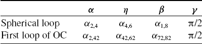
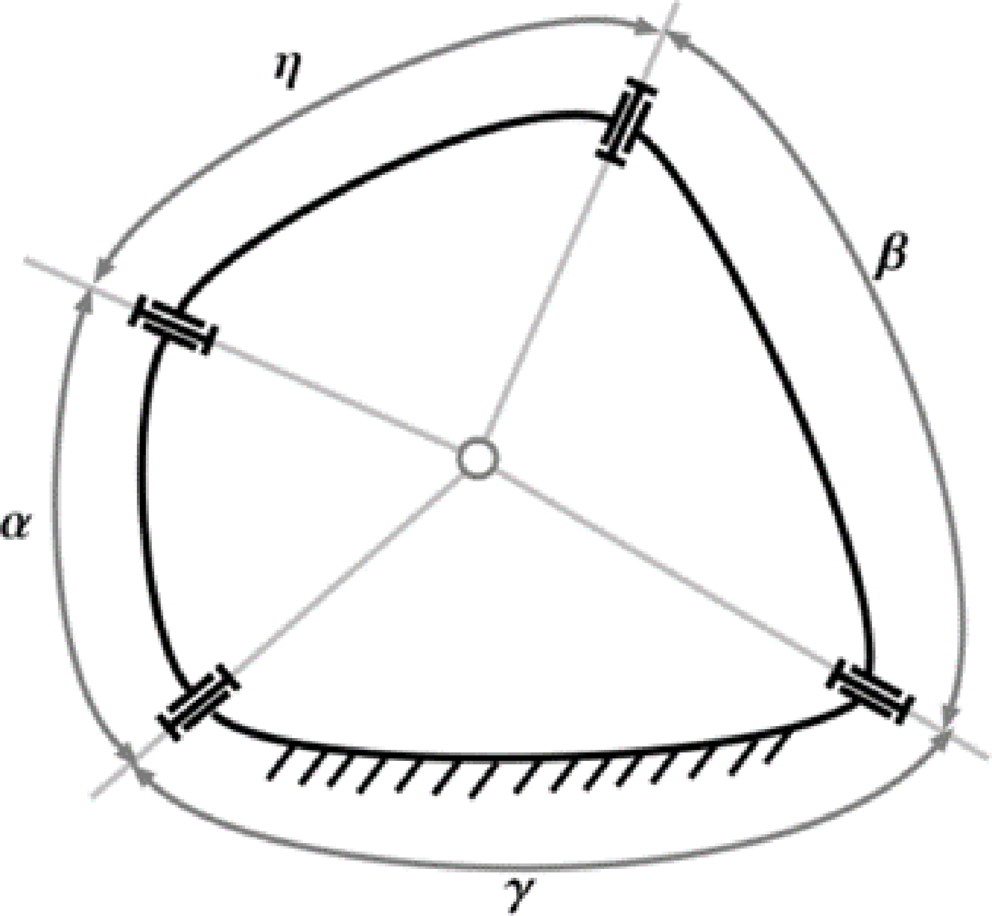
Figure 4. Spherical four-bar mechanism.

C1: $\mathrm{T}_{1}\gt 0\& \mathrm{T}_{2}\gt 0\& \mathrm{T}_{3}\gt 0\& \mathrm{T}_{4}\gt 0$ II $\mathrm{T}_{1}\lt 0\& \mathrm{T}_{2}\lt 0\& \mathrm{T}_{3}\lt 0\& \mathrm{T}_{4}\lt 0$

where

\begin{equation*}\mathrm{T}_{2}=\gamma -\alpha -\eta +\beta, \mathrm{T}_{3}=\eta +\beta -\gamma -\alpha, \mathrm{T}_{4}=2\pi -\eta -\beta -\gamma -\alpha\end{equation*}

5.2.2. Transmission angle

For the sake of torque transmission in the four-bar mechanism, the transmission angle should remain greater than 35° and less than 155° so that it yields to conditions:

C2: $35^{\circ}\lt \alpha _{5,7}\lt 155^{\circ}$ & $35^{\circ}\lt \alpha _{52,72}\lt 155^{\circ}$ & $35^{\circ}\lt \alpha _{95,75}\lt 155^{\circ}$

5.2.3. Design variables range

Spherical mechanisms tend to get into singularity when the value is around 0° or 180°; thus, a range is set as a constraint in the form:

C3: $10^{\circ}\lt \alpha _{i}\lt 170^{\circ}$ or $190^{\circ}\lt \alpha _{i}\lt 350^{\circ}$

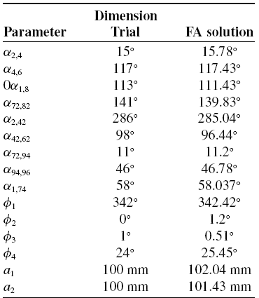
Table IV. Link dimensions by trial and error and after optimized by firefly algorithm.

5.3. Firefly optimization algorithm

In the firefly algorithm, the system’s variables are defined as a vector, and initially, agents (fireflies) are generated. The fireflies propagate lights proportional to the objective function resulting from the variables, and brighter ones pull other fireflies close [43]. Parameters used in the algorithm are selected according to previous research and experiences as reported in ref. [12, 13, 43]. The number of fireflies (n_f) is chosen as 20. The attractiveness (β₀) indicates a firefly’s capability to draw in other fireflies and is selected as 0.8. Randomness (α_r), the probability of random movement, is chosen as 0.2. Scale (S) is selected as 0.1 with intuition. 500 generations are applied. In the algorithm, the light intensity of a firefly is measured by I, and it directly impresses the movement of fireflies. Here, f(x_i) is the objective function, and xi is the vector of parameters that are wanted to be optimized at each iteration. Finally, r_i,j is the monotonically decreasing function of the distance between fireflies. Thus, the algorithm can be expressed as follows:

Generate initial population of fireflies

x_i,i = 1,2,…,n_f

Light intensity I at xi is determined by f(x_i)

Define light absorption coefficient γ

For m = 1, MaxGen

For i = 1: n_f

For j = 1: n_f

If (Ii < Ij); $r_{i,j}=\sqrt{\sum _{k=1}^{n_{c}}(x_{k,i}-x_{k,j})^{2}}$

$x_{k,i}=x_{k,i}+\frac{\beta _{0}S}{1+\gamma r_{i,j}^{2}}\left(x_{k,i}-x_{k,j}\right)+\alpha S \left(Rand\left(\!-.5,.5\right)\right), k=1,n_{c}$ %move firefly i toward j

else $x_{k,i}=x_{k,i}+\alpha S (Rand(\!-.5,.5)), k=1,n_{c}$ %move the brightest firefly randomly

end if

Evaluate new solutions of f(x_i) and update light intensity

end for j

end for i

Rank the fireflies and find the current global best

end for

5.4. Results for dimensional synthesis

Dimensional parameters are obtained after 500 iterations from firefly algorithm as listed in Table IV. In this section, it was checked whether the obtained optimum dimensional parameters provided the desired step profile. Figure 5a illustrates the objective function value with an increasing number of iterations. The results of the optimization demonstrate a significant improvement in the mechanism’s performance, with a 67% reduction in y-direction variation during the drive phase. This improvement was determined by analyzing the vertical deviation, while the input angle changes from 0° to 120°, comparing both the initial trial-and-error solution and the optimized solution. By examining the y-direction variation across this input angle range, the optimization process successfully reduced the vertical deviation, resulting in a smoother and more consistent walking motion.

Figure 5. (a) Firefly optimization by generations, (b) optimized and trial-and-error paths.

6. Simulation result

The simulation step is aimed at verifying the data obtained from the test and to prove the reliability of the method. Walking mechanisms should draw a line as straight as possible in the x-axis direction while touching the ground to move. The dynamic simulation of the models drawn in the CAD (computer-aided design) program is done and simulated using AutoCAD Inventor (Fig. 6).

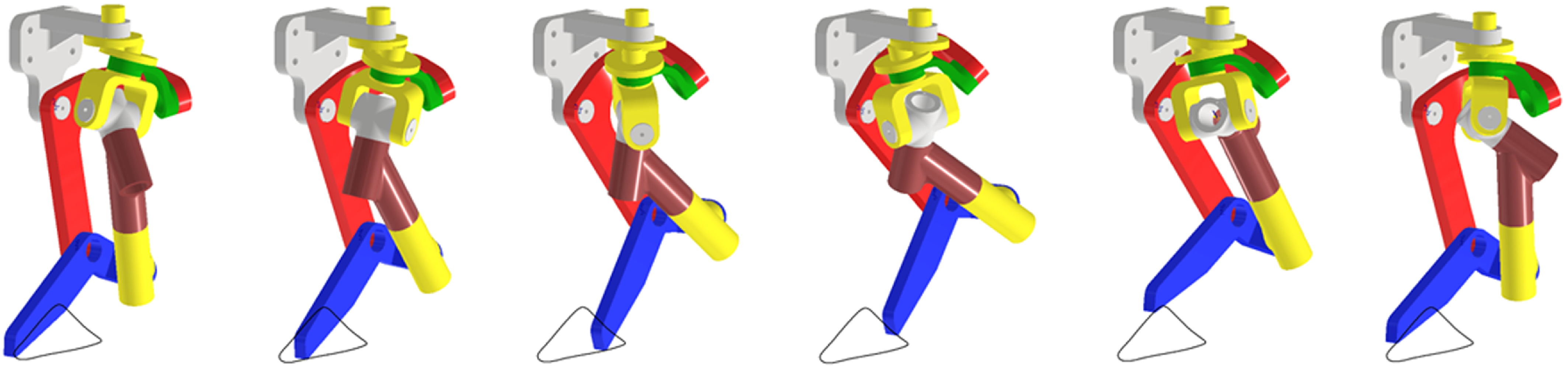
Figure 6. Resulting mechanism after optimization with the simulated path.

In the simulation phase, the initial input speed is given as 72 rad/s. The simulation is completed in two stages. In the first stage, the period of seconds when the mechanism touched the ground is determined. Different approaches are used to determine at which time intervals the mechanism draws a straight line. These are read as the zone where the velocity on the Y-axis is flattest or the zone where the value of Y is constant from the position graph. The time-dependent velocity graph of a moving mechanism on the Y-axis is shown in Fig. 7. Accordingly, from Fig. 7, it is assumed that the mechanism draws a straight line between 1.7 t and 3.6 t because there are fluctuations on Vx while Vy is near zero.

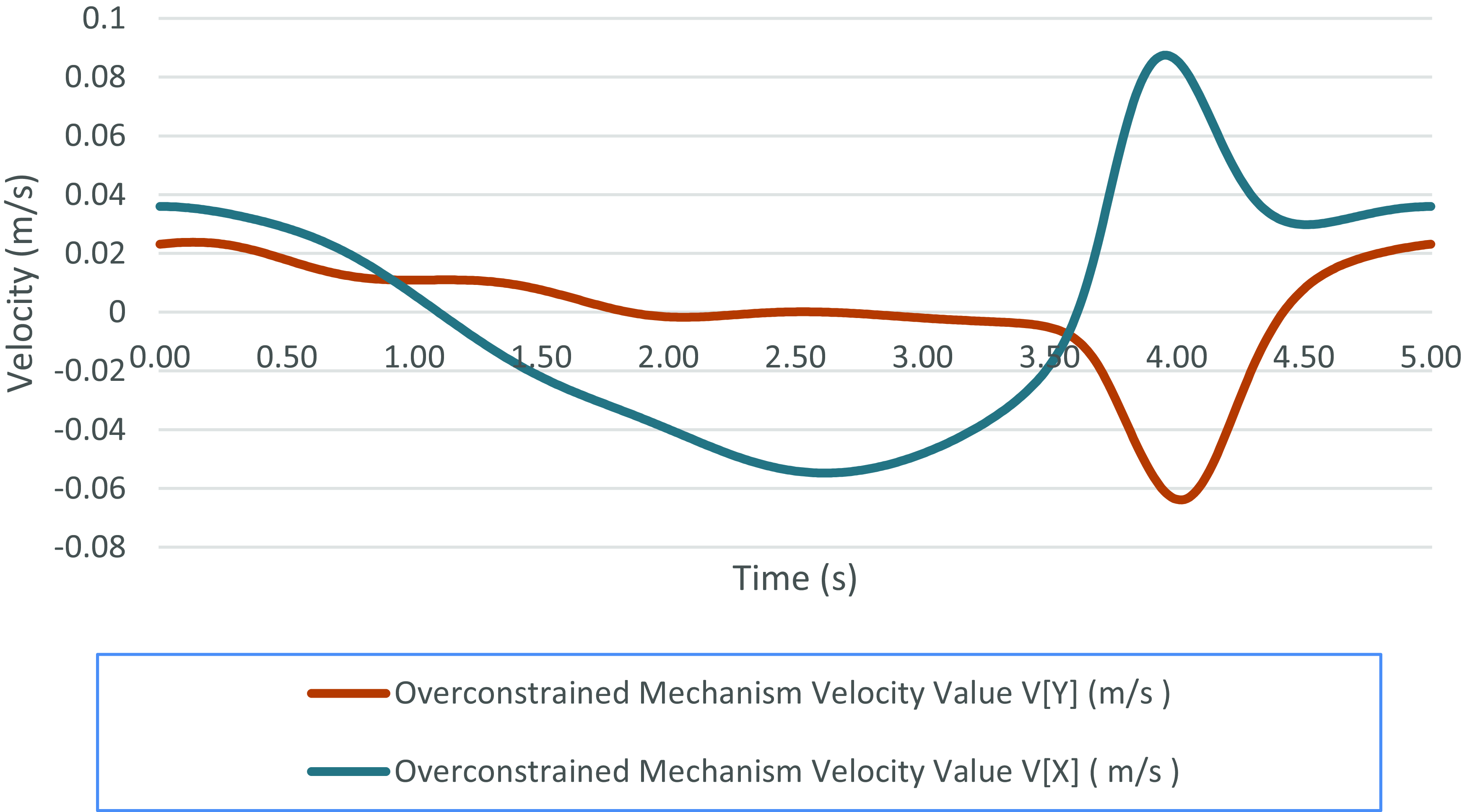
Figure 7. Computed torque in a simulated operation and maximum torque position.

In the second stage, friction force and reaction force are calculated. The robot to be manufactured is aimed to have six legs. All the equipment and the weight of the robot are summed up. During walking, only three legs will touch the ground, so the weight is multiplied by gravity and divided by three. The friction coefficient of the mechanism with the ground is assumed to be 0.9. In this way, the friction force is calculated as 10.7 N. These values are entered into the simulation.

The resultant path of the mechanism in simulation is shown in Fig. 8a. The drive phase of the leg is between 170° and 50° input of the crank. The Lift phase is between 270° and 50°. The return phase is between 235 ° and 270 °. The lowering phase is between 170° and 235°. The path is almost symmetrical concerning the Y-axis. In the drive phase during the stride, it is seen that the y motion is nearly straight. The foot trajectory is also drawn in CAD software and simulated. The comparison with the curve drawn with the analytical solution verifies the result as shown in Fig. 9.

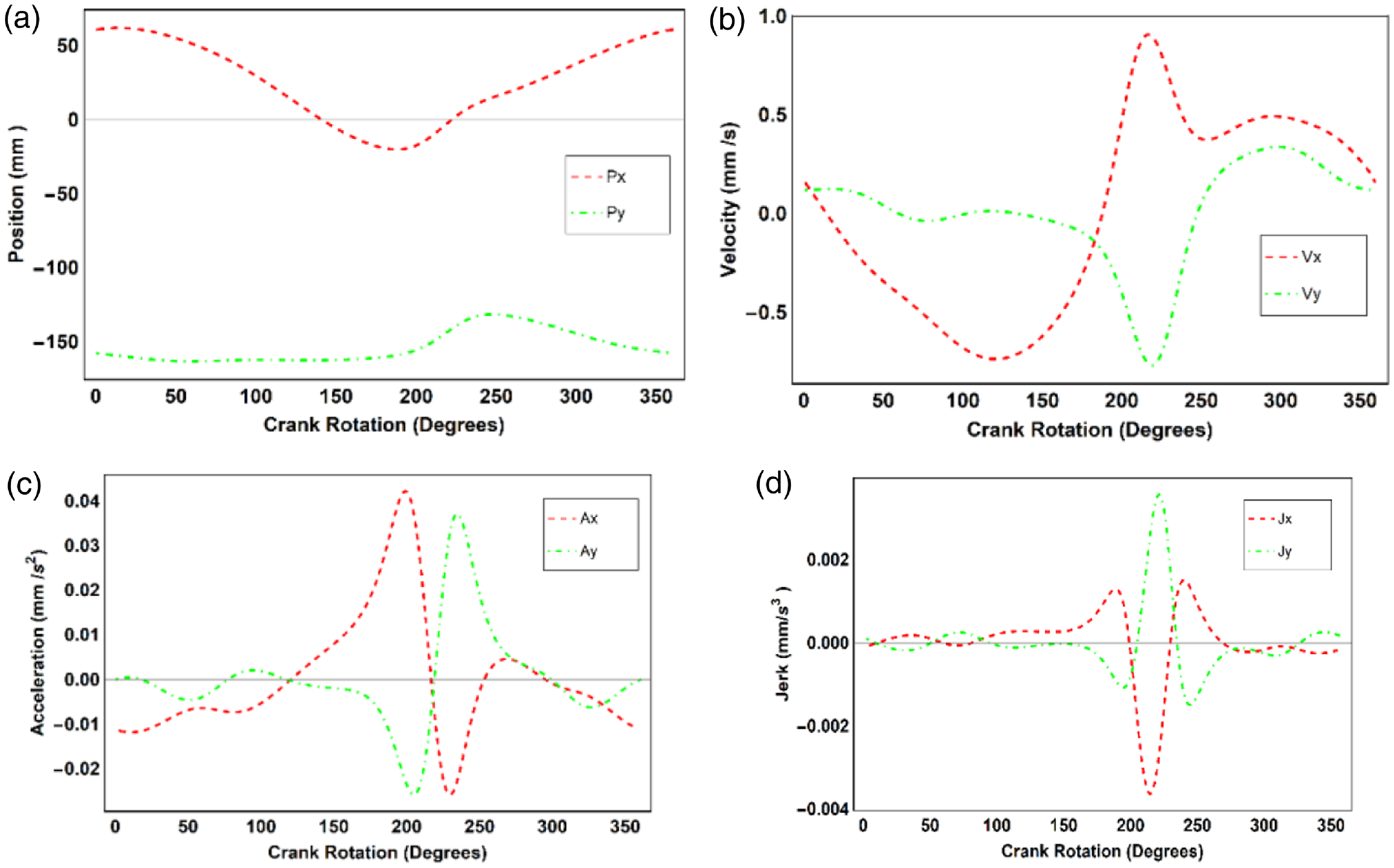
Figure 8. Kinematic results in x and y direction as function of crank rotation: (a) position, (b) velocity, (c) acceleration, (d) jerk.

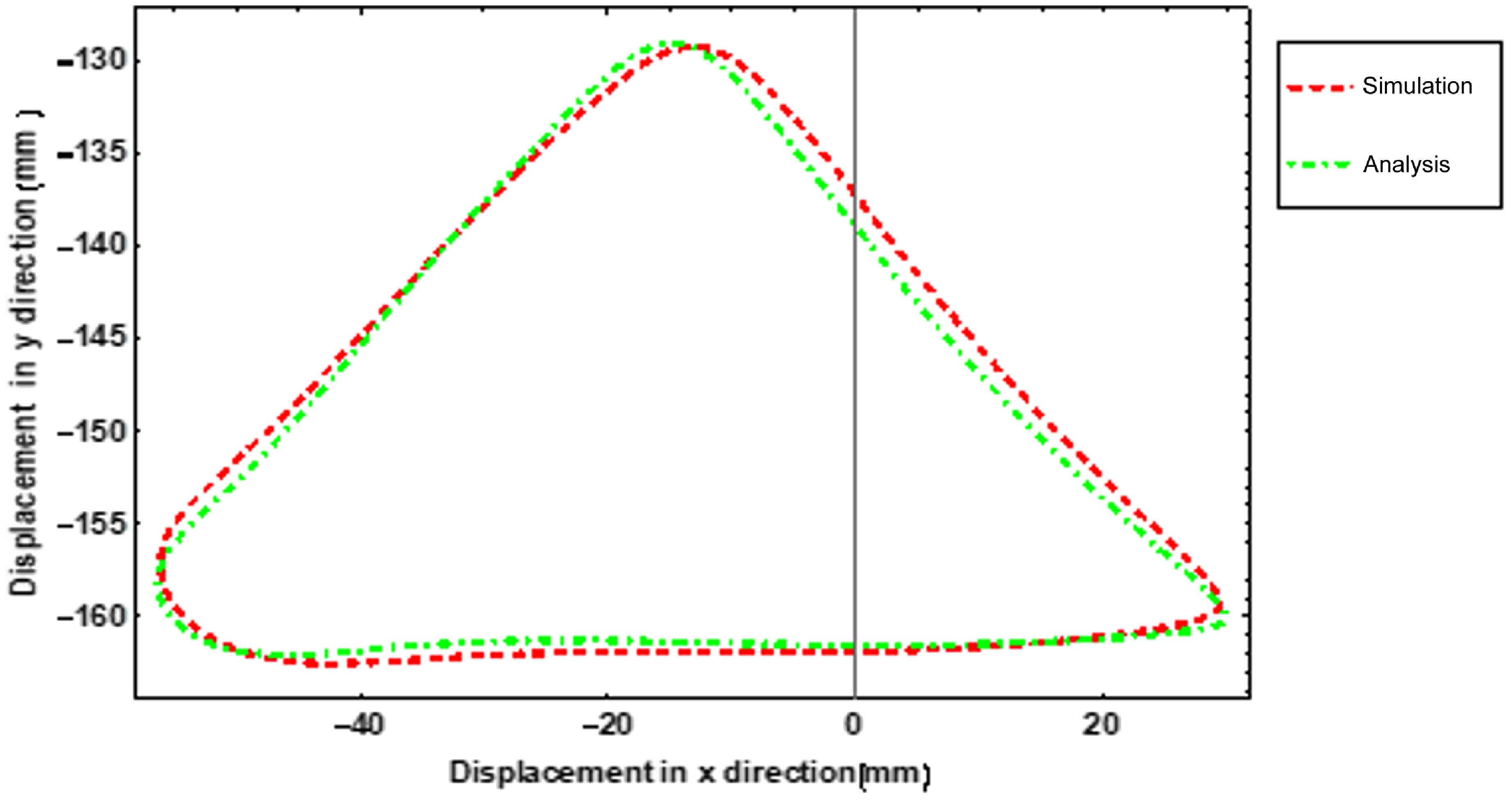
Figure 9. Simulation and analysis result comparison.

Since the increments between the independent variable times are equal, the Richardson method is used for numerical differentiation. The velocity diagram in Fig. 8b shows that velocity in the y direction is almost zero during the drive phase desired in the lift, and in the lower phases, the jerk is high. In the drive phase, the jerk has a low variation (Fig. 8d). At the same time, the end is in the lowering phase between 0° and 50°. During the lowering phase, acceleration is low (Fig. 8c). Thus, the undesirable chance of impact to the ground is softer.

As shown in Fig. 10, the overconstrained walking mechanism is scaled to ×1, ×2, ×4, and ×8 respectively. While scaling, only the dimensions a1 and a2 given in Fig. 2 are changed. Thanks to compact scalability, without scaling the whole mechanism, the walking path increases or decreases at the same rate.

Figure 10. Comparison of the walking paths of mechanisms drawn at different scales.

Figure 11 shows the torque graph obtained for the overconstrained mechanism. According to the torque graph, the force is zero at first, which indicates that the P point of the mechanism, that is, the end part of the foot, is in the air in the initial state. 1.7 s after the motor starts to move, torque is applied for about 2 s when the foot of the mechanism touches the ground. The desired torque value at the top point of the mechanism is approximately 0.52 Nm. The position of the mechanism when it reaches this value is shown in Fig. 11.

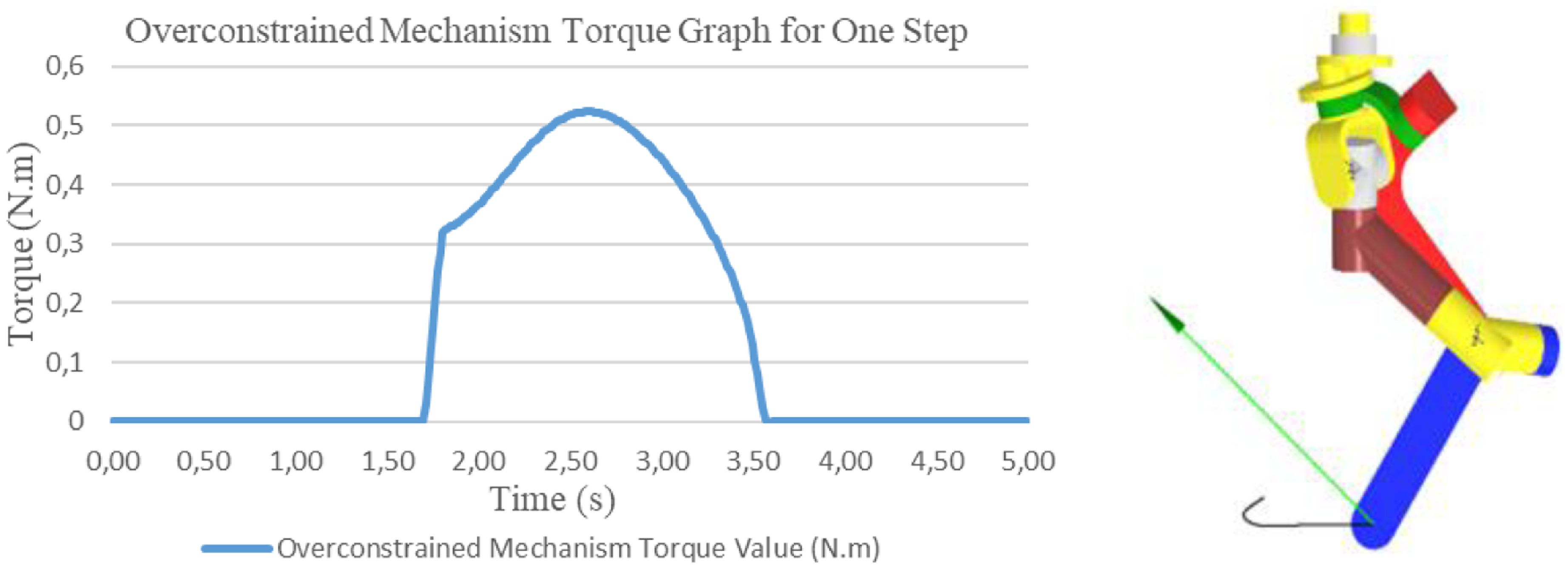
Figure 11. Computed torque in a simulated operation and maximum torque position.

7. Test setup

At this stage, it is aimed to assemble the mechanism to be used in the test setup. The mechanism consists of 13 parts as shown in Fig. 12. These parts are manufactured using a 3D printer with SLA technology. For the mechanism to move, bearings are inserted between the links where one of the links is designed with a pin and the other with a bearing. The bearings and pins are assembled to the links using adhesive, with interference fit.

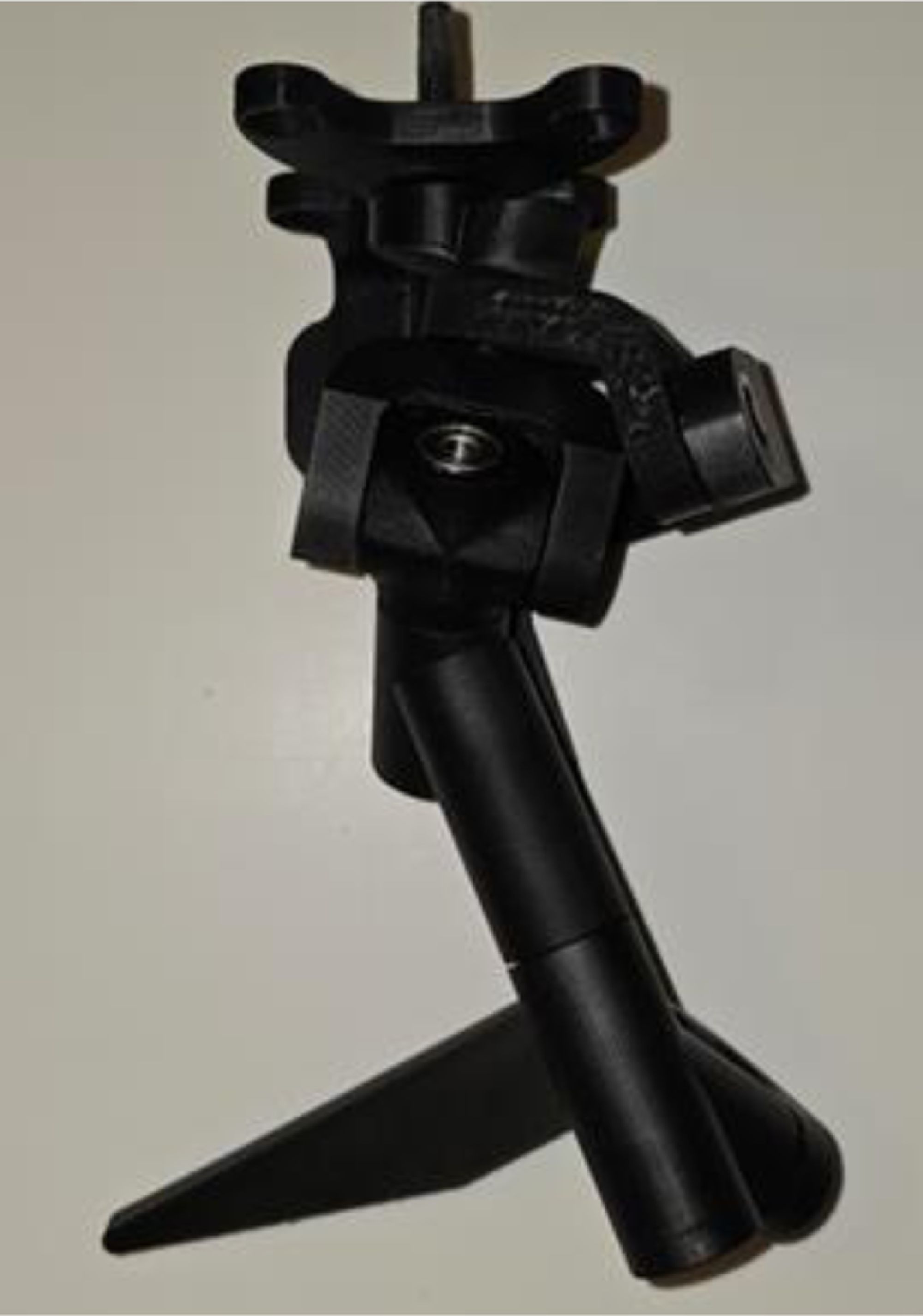
Figure 12. Assembled overconstrained walking mechanism.

A test setup is prepared to compare the simulation and analysis results with test results of the mechanism, as well as to simulate its implementation on a robot as shown in Fig. 13. During the test of the mechanism, it is designed in such a way that it could be elevation-adjustable since it is necessary to have data both while working in the air and on the ground during the test of the mechanism.

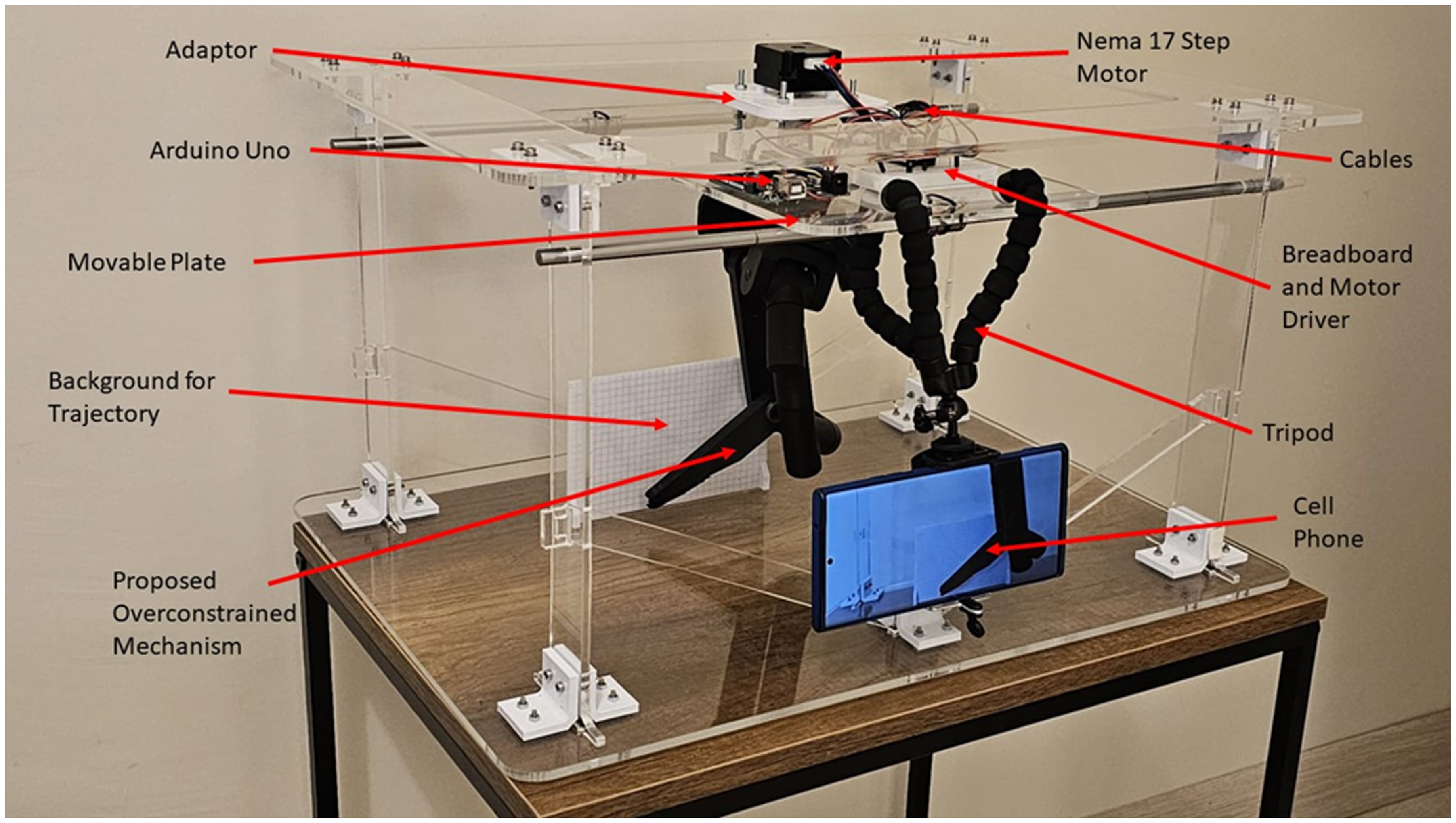
Figure 13. Assembled test setup.

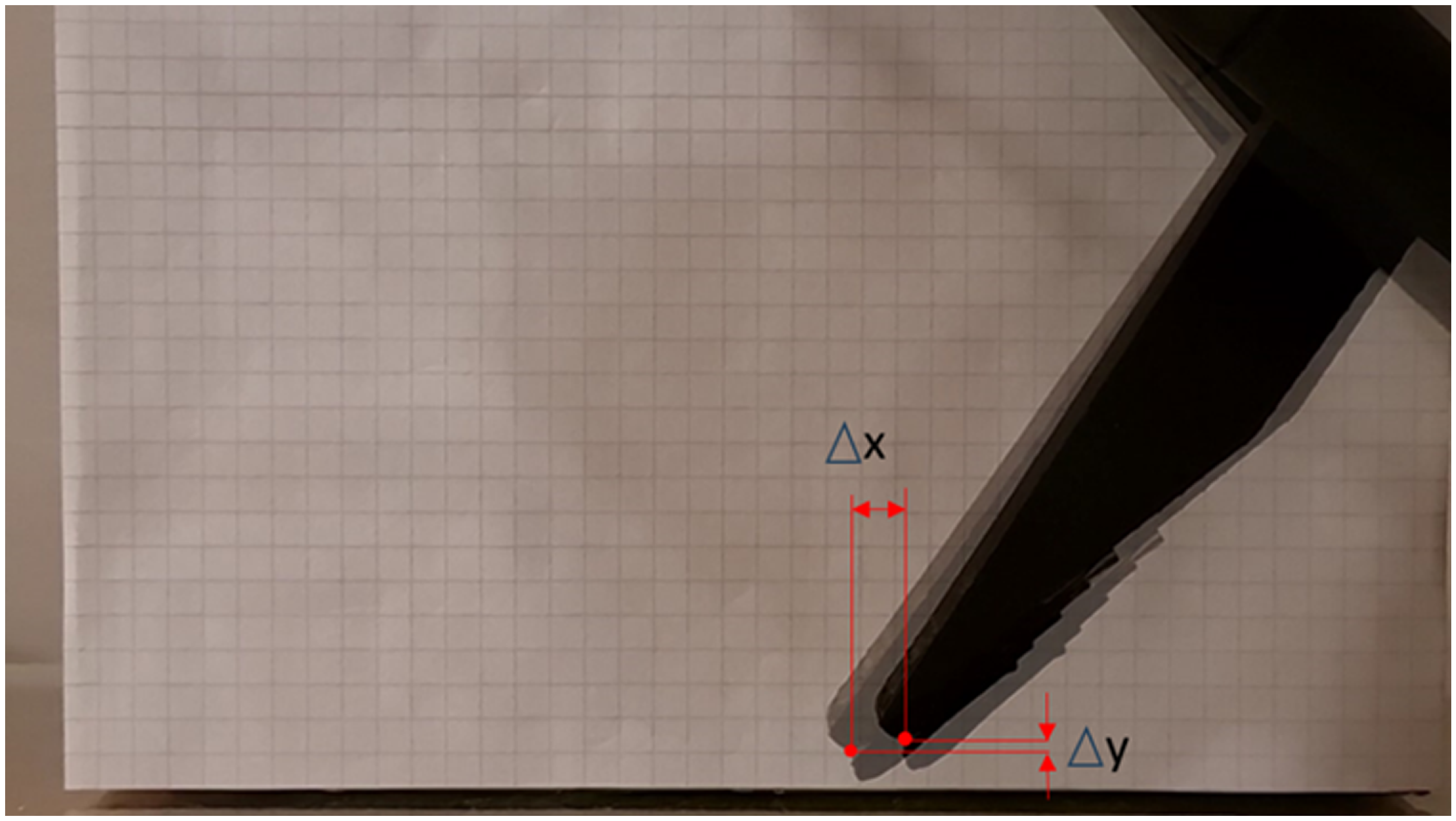
Figure 14. Time-dependent position changes of the mechanism on the X and Y axis.

In designing the test setup, an adaptor moving in the z-axis with the motor is used to adjust the elevation of the mechanism. The mechanism is connected to the stepper motor with a coupling and then to the moving plate with the adaptor. In the case where the mechanism touches the ground, it is aimed to move the foot forward or reverse with the moving plate. The circuit board, motor driver, and cables are placed on the moving plate.

The digital image correlation (tracker) method is used to compare the velocity value of the P point of the mechanism and the walking path with the analysis and simulation data. A camera with 60 fps video recording capability, which has a front view of the mechanism, is attached to the moving plate with the help of a tripod. A background for a trajectory with each square dimension of 5×5 mm is positioned behind the mechanism. In Fig. 14, the initial position of the mechanism is shown in a transparent line, and the final position is shown in a dark color. Since the positions of the mechanism at t_initial and t_final positions are known, it is aimed to extract the time-dependent X and Y graph of the mechanism.

8. Test result

Before checking the numerical accuracy of the experimental setup, the walking path obtained previously is checked. This is also done because the mechanism has more than one walking path. After confirming that the mechanism is in the correct position, the data obtained from the tracker is compared. At the end of the test, the data obtained from dynamic simulation and the data obtained experimentally matched each other.

Figure 15 shows the mechanism’s walking path, which is proven to be in the correct position, obtained by the tracker method. When compared with the walking paths obtained from simulation and analysis in Fig. 9, the walking path of the mechanism is obtained very close to the test result.

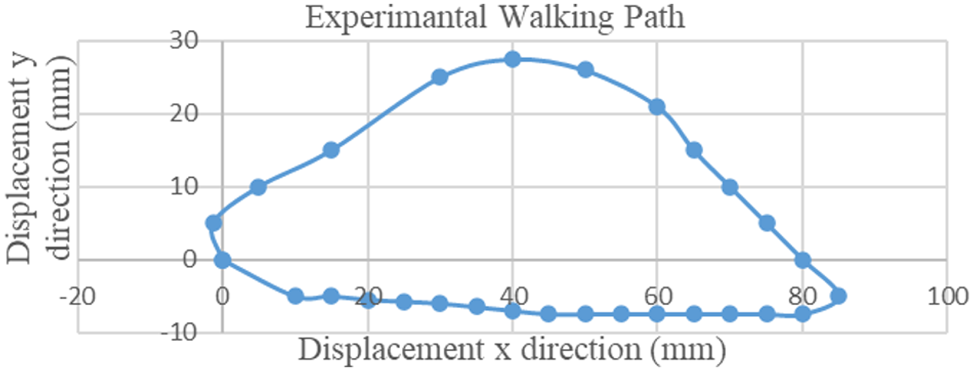
Figure 15. Walking path graph from experiment.

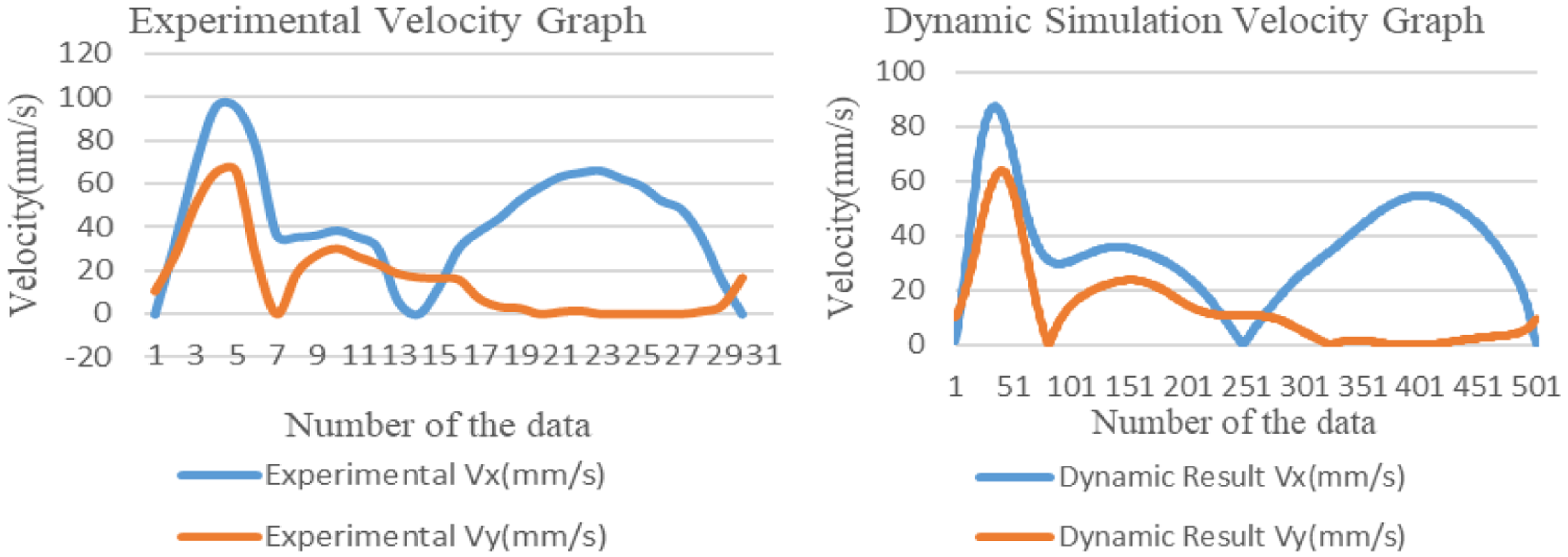
Figure 16. Velocity table comparison between dynamic simulation and experiment.

The difference between the data obtained from the simulation and kinematic analysis and the data obtained from the test setup can be explained in part by manufacturing errors and measuring device errors. Although the mechanism was produced on high-precision 3D printers, the design gaps given during the design phase are large. These design gaps caused a lot of oscillations during the movement of the mechanism. These oscillations also affected the comparison of the speed graphs obtained from the dynamic simulation of the mechanism.

When examining Fig. 16, the speed graphs obtained from the dynamic simulations are shown. A general observation from comparing these two graphs is that they exhibit a similar tendency. However, it becomes apparent that the data collected during the experiment was notably inadequate. This insufficiency in data collection can be attributed as the primary cause for the disparity observed in the dynamic simulation results. The emergence of these differences in the graphs can be attributed to a combination of insufficient data and other errors. Despite these challenges, the data acquired still corroborates the dynamic simulation of the mechanism.

9. Discussion

To observe the differences between the walking mechanisms in the literature and the possible benefits of the proposed overconstrained mechanism, parameters are defined. The comparison subjects are determined by considering the areas of use, assembly, and intended use of the mechanisms.

The main aspects for comparison are the following:

1. 1. Number of Links: It refers to the number of links used during the design of the mechanisms.

2. 2. Number of Joints: It refers to the joints used between the links of the mechanisms.

3. 3. Number of the Supports on the Frame: In order for the mechanism to make the desired movement in the desired plane, it must be fixed from a minimum of two points. This section shows how many points the mechanism is fixed.

4. 4. Compact Scalability: Compact scalability allows reaching the desired scaled walking path by only altering a minimal number of construction parameters.

5. 5. Stride Length Proportion to Body Size: It is the ratio of the distance that the mechanism is considered to be walking, that is, walking in a straight line, to the length of the mechanism. This ratio is changeable due to the compact scalability of the overconstrained mechanism (Fig. 17a).

6. 6. Stride Straightness Ratio Percent: It shows that the mechanism draws a straight line in the walking path it creates, that is, the ratio of the step distance to the path fluctuating height (Fig. 17b).

7. 7. Velocity Profile in the Direction of Stride: It shows the changes in the velocity perpendicular to the velocity of point P in the direction of the stride, that is, during the stride. The smaller the change in velocity perpendicular to the direction of stride, the smoother the straight line formed by the mechanism.

8. 8. Stride to Footprint Ratio Percent: It expresses the ratio of the area covered by the mechanism to the distance the mechanism draws a straight line (Fig. 17c).

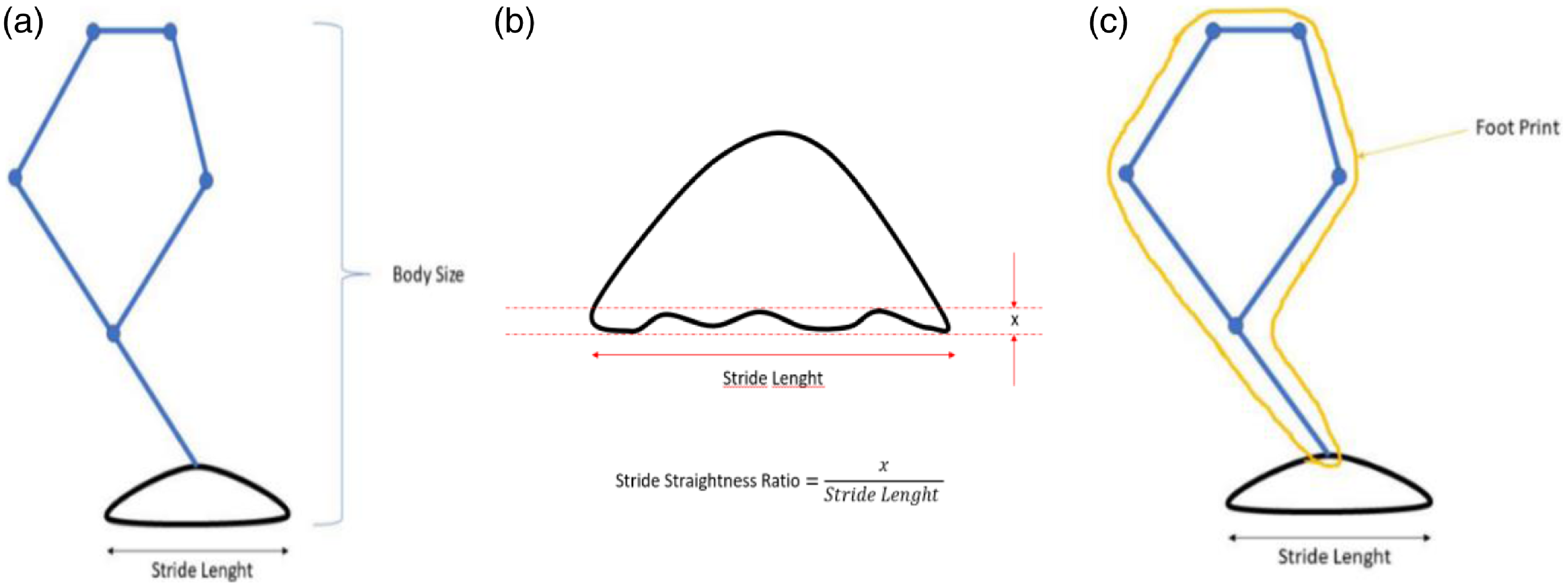
Figure 17. (a) Stride length proportion to body size, (b) stride straightness ratio percent, (c) stride to footprint ratio.

In Table V, The results of the comparisons are shown with the acquired walking path. To ensure that the comparison is made under the same conditions, the mechanism lengths are designed to be the same.

Table V. Comparison of walking mechanisms

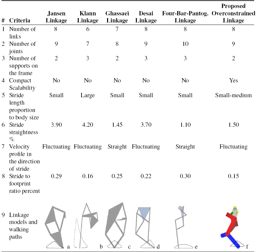
Link lengths related to Jansen’s mechanism are obtained from the work of Theo Jansen [1], Klann’s Linkage is created with parameters from the work of Klann [7], Ghassaei Linkage is derived from the work of Ghassaei et al. [2], Desai Linkage is created according to link lengths given in the work Desai et al. [14], and the parameters of the four-bar pantograph are taken from Ottaviano et al. [19].

As mentioned in the literature survey, the parameters affecting walking are controllable vehicle height, increased traction, climbing capabilities, obstacle-jumping capabilities, etc. The advantages and limitations of these widely used mechanisms are taken into account when making the comparison. The advantages and disadvantages vary depending on the goal to be reached. Jansen Linkage, Klann Linkage, and Desai Linkage are similar in their walking paths, but the distance they take in one step differs. If you want to cover a longer distance in one step, you can choose Jansen Linkage. However, in some cases, the obstacle-jumping capacity may be more important than the walking path. In such a case, the Klann Linkage makes a significant difference compared to other mechanisms. In other situations, the straightness of the mechanism is more important than the distance traveled or the obstacle-jumping capacity. In this case, it is more advantageous to use the Four-Bar Pantograph Linkage than other mechanisms. Comparing the mechanism, we designed with other mechanisms, it has the same walking path as the Jansen Linkage, Klann Linkage, and Desai Linkage mechanisms. However, thanks to its scalability, which we call compact scalability, the whole walking path is scalable and can travel longer. Likewise, thanks to its compact scalability, it can rival the obstacle-jumping capacity of the Klann Linkage mechanism. In addition, because the ratio of the path it takes in one step to the body length is the smallest, the path it travels in proportion to the body length is higher than all other mechanisms. The disadvantages are the high number of links and joints. Another disadvantage is the fluctuations that occur during the walking of the mechanism. However, this is not exactly a disadvantage because the fluctuations are the smallest in the four-bar pantograph mechanism. However, when the mechanism we have designed is compared with the Jansen Linkage, Klann Linkage, and Desai Linkage, the difference between them is negligible.

10. Conclusion

A new overconstrained leg mechanism is presented in this paper. The geometry and the derivation are discussed. The link lengths are designed with optimal values using kinematic analysis for a given objective path with defined constraints. The optimization method is carried out using the firefly algorithm. The designed mechanism has been manufactured and tested.

In terms of compact scalability, which is a characteristic property of the mechanism, different walking paths were derived by changing only three of the eight links. Several linkages from the literature are compared to the proposed mechanism to prove its advantages. It is seen that the proposed mechanisms’ scalability is a benefit. To prove this, four different scales of the mechanism were designed in the dynamic simulation stage, and the walking paths of all of them were demonstrated. It was clearly seen that this mechanism would be more efficient to be used in limited areas, in situations where large or small walking paths need to be obtained.