


1. Introduction
Branched networks for fluid transport are omnipresent in biology and engineering. Biological systems, such as vascular networks (Hutchins, Miner & Boitnott Reference Hutchins, Miner and Boitnott1976; Reichold et al. Reference Reichold, Stampanoni, Keller, Buck, Jenny and Weber2009; Kelch et al. Reference Kelch, Bogle, Sands, Phillips, LeGrice and Rod Dunbar2015) and the bronchial trees of the lungs (Hooper Reference Hooper1977; Xu et al. Reference Xu, Sasmito, Yu and Mujumdar2016; Sznitman Reference Sznitman2022), are capable of efficiently transporting heat or mass with low dissipation within limited volumes (Bejan & Lorente Reference Bejan and Lorente2013). Similarly, fluidic networks provide efficient transport in emerging engineering applications, such as microfluidics (Whitesides Reference Whitesides2006), additive manufacturing (Skylar-Scott et al. Reference Skylar-Scott, Mueller, Visser and Lewis2019; Shaqfeh et al. Reference Shaqfeh, Lipkowitz, Kishna, Coates and DeSimone2023), creation of synthetic vasculatures (Sexton et al. Reference Sexton, Hudson, Herrmann, Shiwarski, Pham, Szafron, Wu, Skylar-Scott, Feinberg and Marsden2023), microreactors (Dong et al. Reference Dong, Wen, Zhao, Kuhn and Noël2021) and multifunctional materials (Zheng et al. Reference Zheng, Shen, Wang, Li, Dunphy, Hasan, Brinker and Su2017). These networks were comprehensively analysed and optimised for Newtonian (Murray Reference Murray1926a ,Reference Murray b ; Kamiya, Togawa & Yamamota Reference Kamiya, Togawa and Yamamota1974; Zamir Reference Zamir1977; Oka & Nakai Reference Oka and Nakai1987), power-law (Mayrovitz Reference Mayrovitz1987; Revellin et al. Reference Revellin, Rousset, Baud and Bonjour2009; Stephenson & Lockerby Reference Stephenson and Lockerby2016; Miguel Reference Miguel2018) and yield-stress fluids (Ponalagusamy Reference Ponalagusamy2012; Smink et al. Reference Smink, Venner, Visser and Hagmeijer2023) in the laminar flow regime. However, a transition to turbulence commonly occurs in natural flows (Olson, Dart & Filley Reference Olson, Dart and Filley1970; Stein & Sabbah Reference Stein and Sabbah1976; Ku Reference Ku1997; Berger & Jou Reference Berger and Jou2000; Calmet et al. Reference Calmet, Gambaruto, Bates, Vázquez, Houzeaux and Doorly2016; Ha et al. Reference Ha, Ziegler, Welander, Bjarnegård, Carlhäll, Lindenberger, Länne, Ebbers and Dyverfeldt2018, Reference Ha, Kvitting, Dyverfeldt and Ebbers2019) and industrial flows such as district heating (Gumpert, Wieland & Spliethoff Reference Gumpert, Wieland and Spliethoff2019; Steinegger et al. Reference Steinegger, Wallner, Greiml and Kienberger2023), water distribution networks, heat exchangers (Siddiqui & Zubair Reference Siddiqui and Zubair2017), the paper making process (Lundell, Söderberg & Alfredsson Reference Lundell, Söderberg and Alfredsson2011) and inertial microfluidics (Wang, Yang & Zhao Reference Wang, Yang and Zhao2014). Similarly, fluidic networks that exhibit both turbulent flow and non-Newtonian behaviour may benefit upscaling of nozzle-based technologies via parallelisation, such as in-air microfluidics (Visser et al. Reference Visser, Kamperman, Karbaat, Lohse and Karperien2018), spray drying (van Deventer, Houben & Koldeweij Reference van Deventer, Houben and Koldeweij2013), prilling (Kamis et al. Reference Kamis, Prakash, Breugem and Eral2023) or 3D printing of polymer foams (Visser et al. Reference Visser, Amato, Mueller and Lewis2019). Finally, analytical optimisation of fluidic networks in various turbulent regimes would provide key validation data for computational fluid dynamics, which is increasingly used to describe (Morris et al. Reference Morris2016) or design (Sexton et al. Reference Sexton, Hudson, Herrmann, Shiwarski, Pham, Szafron, Wu, Skylar-Scott, Feinberg and Marsden2023) networks with e.g. complex geometries.
The parameter space spanned by the Reynolds number, the roughness and different fluid models is shown in figure 1(a,b). Applications are plotted in figure 1(a), showing the broad range of relevant Reynolds numbers, $Re$
, and relative channel wall roughnesses,
$Re$
, and relative channel wall roughnesses, $\delta$
, especially in the intermediate-
$\delta$
, especially in the intermediate- $Re$
turbulent regime (the Reynolds number is defined in (2.4)). Figure 1(b) shows that the energy consumption by the network has been minimised (Murray Reference Murray1926b
; Smink et al. Reference Smink, Venner, Visser and Hagmeijer2023) only for specific limits of this parameter space. This total energy consists of the sum of the power needed to maintain the flow (product of the pressure drop
$Re$
turbulent regime (the Reynolds number is defined in (2.4)). Figure 1(b) shows that the energy consumption by the network has been minimised (Murray Reference Murray1926b
; Smink et al. Reference Smink, Venner, Visser and Hagmeijer2023) only for specific limits of this parameter space. This total energy consists of the sum of the power needed to maintain the flow (product of the pressure drop $\Delta p$
and the volume flow rate
$\Delta p$
and the volume flow rate $Q$
) and a volumetric cost function
$Q$
) and a volumetric cost function $\alpha V$
, with
$\alpha V$
, with $\alpha$
a cost factor and
$\alpha$
a cost factor and $V$
the volume of the channel, for networks as schematically shown in figure 1(c, d). For example, in the case of a vascular network, the cost factor expresses the metabolic energy needed to maintain blood (
$V$
the volume of the channel, for networks as schematically shown in figure 1(c, d). For example, in the case of a vascular network, the cost factor expresses the metabolic energy needed to maintain blood ( $\alpha \approx$
1 kW m
$\alpha \approx$
1 kW m $^{-3}$
) (Murray Reference Murray1926b
); for other situations, see Smink et al. (Reference Smink, Venner, Visser and Hagmeijer2023). Note that optimising the relative channel radii for a given volume is a related problem, which has been pursued for many cases with e.g. a constructional law (Bejan, Rocha L.A. & Lorente Reference Bejan, Rocha L.A. and Lorente2000; Miguel & Rocha Reference Miguel and Rocha2018; Miguel Reference Miguel2018). Instead, we focus on optimisation against a cost factor, which is generalisable for different boundary conditions such as a cost function of the wall surface area (Woldenberg & Horsfield Reference Woldenberg and Horsfield1986) and readily provides access to the optimal channel radii.
$^{-3}$
) (Murray Reference Murray1926b
); for other situations, see Smink et al. (Reference Smink, Venner, Visser and Hagmeijer2023). Note that optimising the relative channel radii for a given volume is a related problem, which has been pursued for many cases with e.g. a constructional law (Bejan, Rocha L.A. & Lorente Reference Bejan, Rocha L.A. and Lorente2000; Miguel & Rocha Reference Miguel and Rocha2018; Miguel Reference Miguel2018). Instead, we focus on optimisation against a cost factor, which is generalisable for different boundary conditions such as a cost function of the wall surface area (Woldenberg & Horsfield Reference Woldenberg and Horsfield1986) and readily provides access to the optimal channel radii.
Figure 1. (a) Parameter space of the Reynolds number $Re$
and the relative channel wall roughness
$Re$
and the relative channel wall roughness $\delta$
for fluidic networks in coronary arteries (Singhal, Henderson & Horsfield Reference Singhal, Henderson and Horsfield1973; Kassab et al. Reference Kassab, Rider, Tang and Fung1993; Burton & Espino Reference Burton and Espino2019), paper making (Forgacs, Robertson & Mason Reference Forgacs, Robertson and Mason1957; Grossman & Carpenter Reference Grossman and Carpenter1968; Moller Reference Moller1976), water distribution (van der Schans et al. Reference van der Schans, Brussee, Niekus and Leunk2015; NEN 2018), inertial microfluidics (Di Carlo Reference Di Carlo2009; Zhang et al. Reference Zhang, Yan, Yuan, Alici, Nguyen, Warkiani and Li2016; Lu et al. Reference Lu, Liu, Hu and Xuan2017), heat exchangers (Towler & Sinnott Reference Towler and Sinnott2013) and district heating (Gumpert et al. Reference Gumpert, Wieland and Spliethoff2019; Steinegger et al. Reference Steinegger, Wallner, Greiml and Kienberger2023). The colour indicates a Newtonian (blue), power-law (green) or yield-stress (red) fluid. Here,
$\delta$
for fluidic networks in coronary arteries (Singhal, Henderson & Horsfield Reference Singhal, Henderson and Horsfield1973; Kassab et al. Reference Kassab, Rider, Tang and Fung1993; Burton & Espino Reference Burton and Espino2019), paper making (Forgacs, Robertson & Mason Reference Forgacs, Robertson and Mason1957; Grossman & Carpenter Reference Grossman and Carpenter1968; Moller Reference Moller1976), water distribution (van der Schans et al. Reference van der Schans, Brussee, Niekus and Leunk2015; NEN 2018), inertial microfluidics (Di Carlo Reference Di Carlo2009; Zhang et al. Reference Zhang, Yan, Yuan, Alici, Nguyen, Warkiani and Li2016; Lu et al. Reference Lu, Liu, Hu and Xuan2017), heat exchangers (Towler & Sinnott Reference Towler and Sinnott2013) and district heating (Gumpert et al. Reference Gumpert, Wieland and Spliethoff2019; Steinegger et al. Reference Steinegger, Wallner, Greiml and Kienberger2023). The colour indicates a Newtonian (blue), power-law (green) or yield-stress (red) fluid. Here, $Re_{crit}$
is assumed to be independent of
$Re_{crit}$
is assumed to be independent of $\delta$
for this parameter space. (b) Previously optimised parts of the parameter space include laminar flow and low-
$\delta$
for this parameter space. (b) Previously optimised parts of the parameter space include laminar flow and low- $Re$
turbulent flow in a smooth channel and a specific condition for complete rough-channel turbulence. (c) Schematic of a single branch with fully developed laminar flow profiles within the channels. (d) Schematic of a branched fluidic network, where a parent channel splits up into
$Re$
turbulent flow in a smooth channel and a specific condition for complete rough-channel turbulence. (c) Schematic of a single branch with fully developed laminar flow profiles within the channels. (d) Schematic of a branched fluidic network, where a parent channel splits up into $N$
daughter channels. The location of the branching point
$N$
daughter channels. The location of the branching point $\boldsymbol{x}$
follows from the analysis and determines the lengths
$\boldsymbol{x}$
follows from the analysis and determines the lengths $L_i$
of the channels. The grey channels indicate that it is possible to have many channels that originate from the branching point. (e, f) Examples of optimised branched fluidic networks. The colour indicates the Reynolds numbers in the channel. The position coordinates of the begin and endnodes are given as an input; the coordinates of intermediate nodes follows from the optimisation. Also the flow rates in all channels are given as an input. The following quantities are kept constant:
$L_i$
of the channels. The grey channels indicate that it is possible to have many channels that originate from the branching point. (e, f) Examples of optimised branched fluidic networks. The colour indicates the Reynolds numbers in the channel. The position coordinates of the begin and endnodes are given as an input; the coordinates of intermediate nodes follows from the optimisation. Also the flow rates in all channels are given as an input. The following quantities are kept constant: $Q_0 = 20$
l min
$Q_0 = 20$
l min $^{-1}$
,
$^{-1}$
, $\rho =1000$
kg m
$\rho =1000$
kg m $^{-3}$
,
$^{-3}$
, $\alpha =10^{3}$
W m
$\alpha =10^{3}$
W m $^{-3}$
and
$^{-3}$
and $\tau _0=0$
Pa. Fluid and system parameters are defined in § 2. (e) Newtonian fluid in rough channel (
$\tau _0=0$
Pa. Fluid and system parameters are defined in § 2. (e) Newtonian fluid in rough channel ( $\mu '=10^{-3}$
Pa s,
$\mu '=10^{-3}$
Pa s, $n=1.0$
,
$n=1.0$
, $\varepsilon = 10^{-5}$
m, 5 levels, symmetric branching). (f) Power-law fluid in smooth channel (
$\varepsilon = 10^{-5}$
m, 5 levels, symmetric branching). (f) Power-law fluid in smooth channel ( $\mu '=5\times 10^{-5}$
Pa s
$\mu '=5\times 10^{-5}$
Pa s $^{1.5}$
,
$^{1.5}$
, $n=1.5$
, 4 levels, asymmetric branching 1:2).
$n=1.5$
, 4 levels, asymmetric branching 1:2).
For a circular pipe with radius $R$
, the power is generally minimised if
$R$
, the power is generally minimised if
 \begin{equation} \frac {R^{x}}{Q} = \text{const.}, \end{equation}
with $x$
a flow-regime and fluid-model-dependent power;
$x$
a flow-regime and fluid-model-dependent power; $x = 3$
for laminar flow of an incompressible Newtonian fluid, as further analysed theoretically (e.g. revealing the shear forces, the optimal angles between channels or special cases such as curved pipes or porous channels) (Kamiya et al. Reference Kamiya, Togawa and Yamamota1974; Zamir Reference Zamir1977; Sherman Reference Sherman1981; Miguel Reference Miguel2018) and verified experimentally for e.g. human coronary and cerebral arteries (Hutchins et al. Reference Hutchins, Miner and Boitnott1976; Rossitti & Löfgren Reference Rossitti and Löfgren1993). The value
$x = 3$
for laminar flow of an incompressible Newtonian fluid, as further analysed theoretically (e.g. revealing the shear forces, the optimal angles between channels or special cases such as curved pipes or porous channels) (Kamiya et al. Reference Kamiya, Togawa and Yamamota1974; Zamir Reference Zamir1977; Sherman Reference Sherman1981; Miguel Reference Miguel2018) and verified experimentally for e.g. human coronary and cerebral arteries (Hutchins et al. Reference Hutchins, Miner and Boitnott1976; Rossitti & Löfgren Reference Rossitti and Löfgren1993). The value $x = 3$
also holds for laminar flows of different fluid models, including power-law (Mayrovitz Reference Mayrovitz1987; Revellin et al. Reference Revellin, Rousset, Baud and Bonjour2009; Stephenson & Lockerby Reference Stephenson and Lockerby2016; Miguel Reference Miguel2018) and yield-stress fluids, such as the Bingham, Herschel–Bulkley and Casson models (Smink et al. Reference Smink, Venner, Visser and Hagmeijer2023), as well as for channels with elliptical (Tesch Reference Tesch2010) and rectangular (Emerson & Barber Reference Emerson and Barber2012), or even arbitrary cross-sections (Emerson et al. Reference Emerson, Cieślicki, Gu and Barber2006; Stephenson et al. Reference Stephenson, Patronis, Holland and Lockerby2015; Zhou et al. Reference Zhou2024).
$x = 3$
also holds for laminar flows of different fluid models, including power-law (Mayrovitz Reference Mayrovitz1987; Revellin et al. Reference Revellin, Rousset, Baud and Bonjour2009; Stephenson & Lockerby Reference Stephenson and Lockerby2016; Miguel Reference Miguel2018) and yield-stress fluids, such as the Bingham, Herschel–Bulkley and Casson models (Smink et al. Reference Smink, Venner, Visser and Hagmeijer2023), as well as for channels with elliptical (Tesch Reference Tesch2010) and rectangular (Emerson & Barber Reference Emerson and Barber2012), or even arbitrary cross-sections (Emerson et al. Reference Emerson, Cieślicki, Gu and Barber2006; Stephenson et al. Reference Stephenson, Patronis, Holland and Lockerby2015; Zhou et al. Reference Zhou2024).
For turbulent flows, fluidic networks were optimised only for limit cases and approximations (Uylings Reference Uylings1977; Woldenberg & Horsfield Reference Woldenberg and Horsfield1986; Bejan et al. Reference Bejan, Rocha L.A. and Lorente2000; Stephenson & Lockerby Reference Stephenson and Lockerby2016). For turbulent flow of Newtonian fluids at intermediate Reynolds numbers $2\times 10^{4} \lt Re\lt 10^{6}$
in a hydraulically smooth channel (shaded for relative wall roughness
$2\times 10^{4} \lt Re\lt 10^{6}$
in a hydraulically smooth channel (shaded for relative wall roughness $\delta \rightarrow 0$
in figure 1
b),
$\delta \rightarrow 0$
in figure 1
b), $x = 17 / 7$
was derived from an empirical relation for the friction factor (Bejan Reference Bejan2013; Kou et al. Reference Kou, Chen, Zhou, Lu, Wu and Fan2014). For complete turbulence (the light-shaded area in figure 1(b), which is defined as
$x = 17 / 7$
was derived from an empirical relation for the friction factor (Bejan Reference Bejan2013; Kou et al. Reference Kou, Chen, Zhou, Lu, Wu and Fan2014). For complete turbulence (the light-shaded area in figure 1(b), which is defined as $Re\gt 3500/\delta$
Moody Reference Moody1944), it was derived that
$Re\gt 3500/\delta$
Moody Reference Moody1944), it was derived that $x = 7 / 3$
(Uylings Reference Uylings1977; Bejan et al. Reference Bejan, Rocha L.A. and Lorente2000; Williams et al. Reference Williams, Trask, Weaver and Bond2008; Stephenson & Lockerby Reference Stephenson and Lockerby2016). Several previous studies (e.g. Revellin et al. Reference Revellin, Rousset, Baud and Bonjour2009 and Zhou et al. Reference Zhou2024) have generalised the optimisation procedure for friction factors that are a power-law function of
$x = 7 / 3$
(Uylings Reference Uylings1977; Bejan et al. Reference Bejan, Rocha L.A. and Lorente2000; Williams et al. Reference Williams, Trask, Weaver and Bond2008; Stephenson & Lockerby Reference Stephenson and Lockerby2016). Several previous studies (e.g. Revellin et al. Reference Revellin, Rousset, Baud and Bonjour2009 and Zhou et al. Reference Zhou2024) have generalised the optimisation procedure for friction factors that are a power-law function of $R$
, and show that all these limit cases can be described by a single approach. However, the intermediate part of the parameter space is described by more complex friction factors that cannot be implemented in these existing approaches, such as the Colebrook–White equation. Stephenson et al. (Reference Stephenson, Patronis, Holland and Lockerby2015) and Stephenson & Lockerby (Reference Stephenson and Lockerby2016) use a different approach allowing friction factors in arbitrary functional form, but they do not apply this to the intermediate part of the parameter space. This terra incognita represents a major knowledge gap, both fundamentally, as it covers several orders of magnitude of both
$R$
, and show that all these limit cases can be described by a single approach. However, the intermediate part of the parameter space is described by more complex friction factors that cannot be implemented in these existing approaches, such as the Colebrook–White equation. Stephenson et al. (Reference Stephenson, Patronis, Holland and Lockerby2015) and Stephenson & Lockerby (Reference Stephenson and Lockerby2016) use a different approach allowing friction factors in arbitrary functional form, but they do not apply this to the intermediate part of the parameter space. This terra incognita represents a major knowledge gap, both fundamentally, as it covers several orders of magnitude of both $Re$
and
$Re$
and $\delta$
, and from an application perspective, as we will show that turbulent limit cases are rarely reached for realistic flows.
$\delta$
, and from an application perspective, as we will show that turbulent limit cases are rarely reached for realistic flows.
In this study, we introduce a universal approach for optimising fluidic networks in the entire parameter space. The optimisation procedure is applicable to any flow regime, wall roughness or fluid model for which the Darcy friction factor is known, even if its formulation is implicit. First, § 2 describes non-dimensionalisation of pipe flows, enabling calculation of the optimal Reynolds number within a channel and the corresponding channel radius. Subsequently, the optimal channel radius is derived for laminar and turbulent flow at arbitrary $Re$
, arbitrary channel roughness
$Re$
, arbitrary channel roughness $\delta$
and for both Newtonian and non-Newtonian fluids in § 3. Section 4 synthesises the results from §§ 2 and 3, resulting in approximations of
$\delta$
and for both Newtonian and non-Newtonian fluids in § 3. Section 4 synthesises the results from §§ 2 and 3, resulting in approximations of $x$
as a function of
$x$
as a function of $Re$
for all flow regimes and fluid models. The design procedure is presented in § 5. The conclusions are presented in § 6. The design of the optimal location of branching points within the network is described in Appendix A.1, resulting in fully optimised networks for e.g. rough-wall channels (figure 1
e) or for non-Newtonian fluids (figure 1
f). Finally, an application example is provided in Appendix F.
$Re$
for all flow regimes and fluid models. The design procedure is presented in § 5. The conclusions are presented in § 6. The design of the optimal location of branching points within the network is described in Appendix A.1, resulting in fully optimised networks for e.g. rough-wall channels (figure 1
e) or for non-Newtonian fluids (figure 1
f). Finally, an application example is provided in Appendix F.
2. Optimisation of fluidic branching
Consider a branching configuration comprising a parent channel connected to $N$
daughter channels at a branching point denoted as
$N$
daughter channels at a branching point denoted as $\boldsymbol{x}$
, as depicted in figure 1(d). The channels are labelled
$\boldsymbol{x}$
, as depicted in figure 1(d). The channels are labelled $0$
to
$0$
to $N$
, with index
$N$
, with index $0$
indicating the parent channel. The effective radii of the channels are represented as
$0$
indicating the parent channel. The effective radii of the channels are represented as $\boldsymbol{R}\equiv (R_0, R_1,\ldots, R_N)$
, while the termination points of the channels are fixed and denoted as
$\boldsymbol{R}\equiv (R_0, R_1,\ldots, R_N)$
, while the termination points of the channels are fixed and denoted as $\boldsymbol{x}_i$
for
$\boldsymbol{x}_i$
for $i=0,1,\ldots, N$
. The flow rates in the daughter channels are specified as
$i=0,1,\ldots, N$
. The flow rates in the daughter channels are specified as $Q_i$
for
$Q_i$
for $i=1,\ldots, N$
, with
$i=1,\ldots, N$
, with $Q_0$
corresponding to the flow rate in the parent channel;
$Q_0$
corresponding to the flow rate in the parent channel; $Q_0$
is considered positive towards the branching point, whereas the flow rates in the daughter channels (
$Q_0$
is considered positive towards the branching point, whereas the flow rates in the daughter channels ( $Q_i$
,
$Q_i$
, $i=1,\ldots, N$
) are taken positive away from the branching point. To ensure mass conservation, assuming incompressibility, the flow rates must satisfy
$i=1,\ldots, N$
) are taken positive away from the branching point. To ensure mass conservation, assuming incompressibility, the flow rates must satisfy $Q_0=\sum _{i=1}^{N} Q_i.$
The lengths of the channels,
$Q_0=\sum _{i=1}^{N} Q_i.$
The lengths of the channels, $L_i$
, are functions of the branching location, given by
$L_i$
, are functions of the branching location, given by $L_i\equiv |\boldsymbol{x}_i-\boldsymbol{x}|$
for
$L_i\equiv |\boldsymbol{x}_i-\boldsymbol{x}|$
for $i=0,1,\ldots, N$
. In this work, it is assumed that there is only an axial velocity
$i=0,1,\ldots, N$
. In this work, it is assumed that there is only an axial velocity $u$
. The channels are assumed to be cylindrical with
$u$
. The channels are assumed to be cylindrical with $R\ll L$
. The fluid properties are taken constant and the flow is fully developed.
$R\ll L$
. The fluid properties are taken constant and the flow is fully developed.
For optimisation of a fluidic network, the power to maintain the flow and to maintain a fluid is minimised. The power is represented by a cost function depending on the radii and lengths of the channels, and is the sum of the individual channel contributions
 \begin{equation} P(\boldsymbol{R},\boldsymbol{x}) \equiv \sum _{i=0}^{N} \left (\Delta p_i\, Q_i + \alpha V_i\right ). \end{equation}
Here, $V_i \equiv \pi R_i^{2} L_i$
is the channel volume and the pressure gradient
$V_i \equiv \pi R_i^{2} L_i$
is the channel volume and the pressure gradient ${\Delta p}/{L}$
is a fluid-type and flow-regime-dependent function. The pressure at the nodes is not defined or constrained. Differentiation of (2.1) to
${\Delta p}/{L}$
is a fluid-type and flow-regime-dependent function. The pressure at the nodes is not defined or constrained. Differentiation of (2.1) to $\boldsymbol{R}$
and
$\boldsymbol{R}$
and $\boldsymbol{x}$
and equating these expressions to 0 provides the optimisation problems for: (i) the channel radii
$\boldsymbol{x}$
and equating these expressions to 0 provides the optimisation problems for: (i) the channel radii $\boldsymbol{R}$
, and (ii) the location of the branching point
$\boldsymbol{R}$
, and (ii) the location of the branching point $\boldsymbol{x}$
(optimised in Appendix A.1). Optimisation of the channel radius is independent of
$\boldsymbol{x}$
(optimised in Appendix A.1). Optimisation of the channel radius is independent of $\boldsymbol{x}$
, because it is a decoupled problem (Smink et al. Reference Smink, Venner, Visser and Hagmeijer2023), in which the power defined by (2.1) attains a global minimum with respect to the radius if all channels satisfy
$\boldsymbol{x}$
, because it is a decoupled problem (Smink et al. Reference Smink, Venner, Visser and Hagmeijer2023), in which the power defined by (2.1) attains a global minimum with respect to the radius if all channels satisfy ${\partial P}/{\partial \boldsymbol{R}}=\boldsymbol{0}$
. Therefore, the optimisation condition for any radius
${\partial P}/{\partial \boldsymbol{R}}=\boldsymbol{0}$
. Therefore, the optimisation condition for any radius $R_i$
only depends on the power contribution of the corresponding channel and
$R_i$
only depends on the power contribution of the corresponding channel and $R_i$
does not depend on the lengths of the channels
$R_i$
does not depend on the lengths of the channels $L_i$
.
$L_i$
.
For minimising the power consumption in the network, every single channel has to be optimised individually according to
 \begin{equation} \frac {\partial {P}}{\partial {R_i}}=\frac {\partial {\Delta p_i}}{\partial {R_i}}Q_i+2\pi \alpha R_iL_i=0, \quad i=0,1,\ldots, N. \end{equation}
The pressure drop $\Delta p$
is represented as a function of a flow rate
$\Delta p$
is represented as a function of a flow rate $Q$
and a radius
$Q$
and a radius $R$
using the Darcy–Weisbach equation (Weisbach Reference Weisbach1845)
$R$
using the Darcy–Weisbach equation (Weisbach Reference Weisbach1845)
 \begin{equation} \Delta p = f\, \frac {\rho }{4\pi ^{2}}\frac {Q^{2}}{R^{5}}L. \end{equation}
Here, $\rho$
is the fluid density,
$\rho$
is the fluid density, $L$
is the length of the channel and
$L$
is the length of the channel and $f$
the Darcy friction factor. The friction factor
$f$
the Darcy friction factor. The friction factor $f$
as function of the Reynolds number for the different fluid models is presented in figures 2(b)–2(d). The specific equations of
$f$
as function of the Reynolds number for the different fluid models is presented in figures 2(b)–2(d). The specific equations of $f$
for different flow regimes and fluid models are provided in § 3. In this study, a generalised Reynolds number is defined as (Garcia & Steffe Reference Garcia and Steffe1986)
$f$
for different flow regimes and fluid models are provided in § 3. In this study, a generalised Reynolds number is defined as (Garcia & Steffe Reference Garcia and Steffe1986)
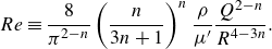 \begin{equation} Re\equiv \frac {8}{\pi ^{2-n}}\left (\frac {n}{3n+1}\right )^{n}\frac {\rho }{\mu '}\frac {Q^{2-n}}{R^{4-3n}}. \end{equation}
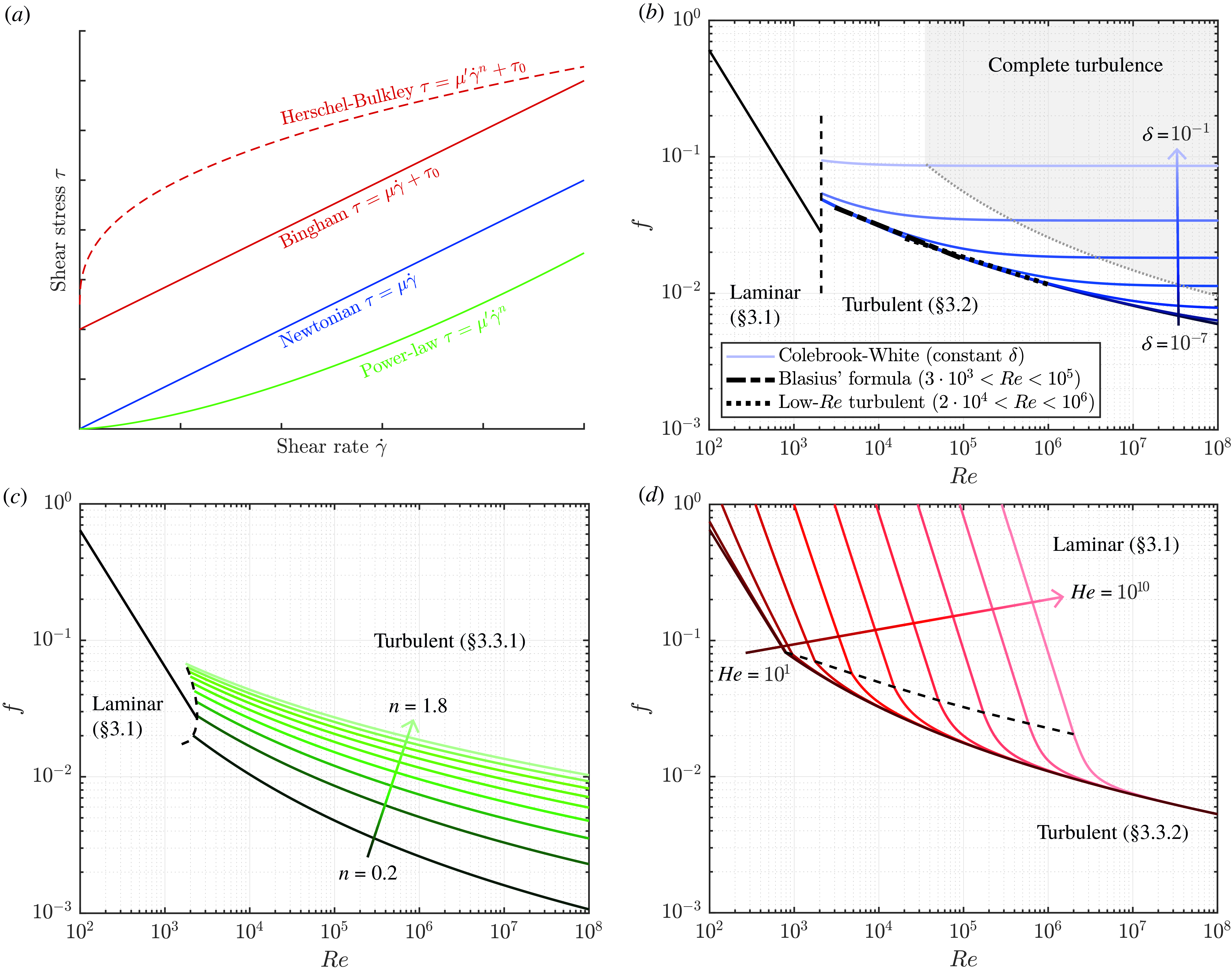
Figure 2. (a) Fluid models as analysed in this work. (b–d) Friction factor as function of the Reynolds number for different fluid models. The dashed black line indicates the transition from laminar to turbulent flow. (b) Newtonian fluid in rough channels (Moody diagram (Moody Reference Moody1944)). The blue lines represent constant relative roughness $\delta$
from
$\delta$
from $10^{-7}, 10^{-6}, \ldots 10^{-1}$
. (c) Power-law fluid in smooth channels. The green-scale lines represent values of the flow index
$10^{-7}, 10^{-6}, \ldots 10^{-1}$
. (c) Power-law fluid in smooth channels. The green-scale lines represent values of the flow index $n$
from
$n$
from $0.2, 0.4, \ldots 1.8$
. (d) Herschel–Bulkley fluid with
$0.2, 0.4, \ldots 1.8$
. (d) Herschel–Bulkley fluid with $n=1.0$
in smooth channels. the red-scale lines represent constant values of the Hedström number from
$n=1.0$
in smooth channels. the red-scale lines represent constant values of the Hedström number from $10^{1}, 10^{2}, \ldots, 10^{10}$
.
$10^{1}, 10^{2}, \ldots, 10^{10}$
.
The value of $f$
also depends on the Hedström number
$f$
also depends on the Hedström number $He$
(commonly used for description of yield-stress fluids), the relative wall roughness
$He$
(commonly used for description of yield-stress fluids), the relative wall roughness $\delta \equiv \varepsilon /2R$
(where
$\delta \equiv \varepsilon /2R$
(where $\varepsilon$
is the absolute channel wall roughness) and the flow index
$\varepsilon$
is the absolute channel wall roughness) and the flow index $n$
.
$n$
.
The effective dynamic viscosity $\mu$
describes the resistance of a fluid against shear, and is defined as
$\mu$
describes the resistance of a fluid against shear, and is defined as $\mu = \mu '|\dot {\gamma }|^{n-1}$
, where
$\mu = \mu '|\dot {\gamma }|^{n-1}$
, where $\dot {\gamma }$
is the shear rate,
$\dot {\gamma }$
is the shear rate, $\mu '$
is the flow consistency index and
$\mu '$
is the flow consistency index and $n$
the flow index, where
$n$
the flow index, where $0\lt n\lt 1$
represents a shear-thinning and
$0\lt n\lt 1$
represents a shear-thinning and $n\gt 1$
represents a shear-thickening fluid, as shown in figure 2(a). In addition, a fluid may show yield-stress behaviour if
$n\gt 1$
represents a shear-thickening fluid, as shown in figure 2(a). In addition, a fluid may show yield-stress behaviour if $\tau _0\geqslant 0$
(e.g. Bingham and Herschel–Bulkley fluids, see figure 2
a), where the fluid only shears once an effective local shear stress exceeds the yield stress
$\tau _0\geqslant 0$
(e.g. Bingham and Herschel–Bulkley fluids, see figure 2
a), where the fluid only shears once an effective local shear stress exceeds the yield stress $\tau _0$
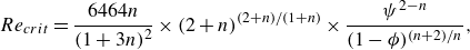
. The rheological behaviour for the shear rate of a Herschel–Bulkley fluid as function of the effective local shear stress is described as
$\tau _0$
. The rheological behaviour for the shear rate of a Herschel–Bulkley fluid as function of the effective local shear stress is described as
 \begin{equation} \dot {\gamma }(\tau ) = \begin{cases} \text{sign}(\tau _{rz})\left ( \frac {|\tau _{rz}|-\tau _0}{\mu '} \right )^{1/n} & \text{if $|\tau _{rz}|\geqslant \tau _0$},\\ 0 & \text{if $|\tau _{rz}|\lt \tau _0$},\\ \end{cases} \end{equation}
where $\tau _{rz}$
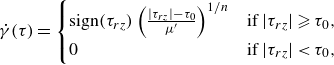
is the local shear stress induced by the flow. Figures 2(b)–2(d) also show the transition from laminar to turbulent flows at the critical Reynolds number (Hanks & Ricks Reference Hanks and Ricks1974)
$\tau _{rz}$
is the local shear stress induced by the flow. Figures 2(b)–2(d) also show the transition from laminar to turbulent flows at the critical Reynolds number (Hanks & Ricks Reference Hanks and Ricks1974)
 \begin{equation} Re_{crit} = \frac {6464n}{(1+3n)^{2}}\times (2+n)^{(2+n)/(1+n)}\times \frac {\psi ^{2-n}}{(1-\phi )^{(n+2)/n}}, \end{equation}
where $\psi (\phi, n)$
and
$\psi (\phi, n)$
and $\phi$
are defined in § 3.1. Although an increased relative roughness results in a decrease in
$\phi$
are defined in § 3.1. Although an increased relative roughness results in a decrease in $Re_{crit}$
, this effect becomes only dominant around
$Re_{crit}$
, this effect becomes only dominant around $\delta =0.1$
and larger (Everts, Robbertse & Spitholt Reference Everts, Robbertse and Spitholt2022). In order to ensure the validity of the used equations, the present study will limit the discussed optimisation results to
$\delta =0.1$
and larger (Everts, Robbertse & Spitholt Reference Everts, Robbertse and Spitholt2022). In order to ensure the validity of the used equations, the present study will limit the discussed optimisation results to $\delta \leqslant 0.1$
.
$\delta \leqslant 0.1$
.
The optimisation condition for the radius of every channel is obtained by substituting (2.3) into (2.2), providing
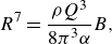 \begin{equation} R^{7}=\frac {\rho Q^{3}}{8\pi ^{3}\alpha } B, \end{equation}
where $B$
is defined as
$B$
is defined as
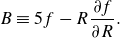 \begin{equation} B \equiv 5f -R\frac {\partial {f}}{\partial {R}}. \end{equation}
Here, $B$
is a function of
$B$
is a function of $f$
and
$f$
and $R$
and thus indirectly also a function of
$R$
and thus indirectly also a function of $Re$
,
$Re$
, $He$
,
$He$
, $\delta$
and
$\delta$
and $n$
.
$n$
.
The goal is to obtain an expression for the optimal channel radius as a function of parameters that are independent of $R$
. Therefore, dimensional analysis is carried out to find a dimensionless form of the channel radius as function of radius-independent dimensionless groups (for more details, see Appendix A.2). Scaling of the optimisation problem results in the following 5 dimensionless numbers:
$R$
. Therefore, dimensional analysis is carried out to find a dimensionless form of the channel radius as function of radius-independent dimensionless groups (for more details, see Appendix A.2). Scaling of the optimisation problem results in the following 5 dimensionless numbers:
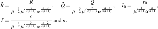 \begin{align} \tilde {R} &\equiv \frac {R}{\rho ^{-\frac {1}{2}} \mu ^{\prime \frac {3}{2(n+1)}} \alpha ^{\frac {n-2}{2(n+1)}}},\quad \tilde {Q} \equiv \frac {Q}{\rho ^{-\frac {3}{2}} \mu ^{\prime \frac {7}{2(n+1)}} \alpha ^{\frac {3n-4}{2(n+1)}}},\quad \tilde {\tau }_0 \equiv \frac {\tau _0}{\mu ^{\prime \frac {1}{n+1}} \alpha ^{\frac {n}{n+1}}}, \nonumber\\\tilde {\varepsilon } & \equiv \frac {\varepsilon }{\rho ^{-\frac {1}{2}} \mu ^{\prime \frac {3}{2(n+1)}} \alpha ^{\frac {n-2}{2(n+1)}}} \text{ and } n .\end{align}
To align with the literature, the Reynolds number will be used instead of $\tilde {R}$
. This choice will simplify the later computations in § 3 and enables direct characterisation of the flow in the channel. The Reynolds number is rewritten in dimensionless groups as follows:
$\tilde {R}$
. This choice will simplify the later computations in § 3 and enables direct characterisation of the flow in the channel. The Reynolds number is rewritten in dimensionless groups as follows:
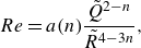 \begin{equation} Re=a(n)\frac {\tilde {Q}^{2-n}}{\tilde {R}^{4-3n}}, \end{equation}
where $a(n)$
is defined as
$a(n)$
is defined as
 \begin{equation} a(n) \equiv \frac {8}{\pi ^{2-n}}\left (\frac {n}{3n+1}\right )^n. \end{equation}
The network is described by the dimensionless numbers $Re$
,
$Re$
, $\tilde {Q}$
,
$\tilde {Q}$
, $\tilde {\tau }_0$
,
$\tilde {\tau }_0$
, $\tilde {\varepsilon }$
and
$\tilde {\varepsilon }$
and $n$
. As
$n$
. As $\tilde {\tau }_0$
,
$\tilde {\tau }_0$
, $\tilde {\varepsilon }$
and
$\tilde {\varepsilon }$
and $n$
are fluid or system parameters that are constant in a network,
$n$
are fluid or system parameters that are constant in a network, $Re$
and
$Re$
and $\tilde {Q}$
are the only flow-rate-dependent dimensionless numbers, which is convenient for network optimisation. Described with the new dimensionless numbers,
$\tilde {Q}$
are the only flow-rate-dependent dimensionless numbers, which is convenient for network optimisation. Described with the new dimensionless numbers, $f$
will now be a function of 5 dimensionless numbers instead of 4. Therefore, in the new domain, there will be a curve along which
$f$
will now be a function of 5 dimensionless numbers instead of 4. Therefore, in the new domain, there will be a curve along which $f$
is constant, removing one degree of freedom (see Appendix A.3).
$f$
is constant, removing one degree of freedom (see Appendix A.3).
For given fluid, flow and system properties, an optimal channel radius can be calculated via the Reynolds number using the non-dimensionalised optimisation condition (2.7)
 \begin{equation} (8\pi ^{3})^{4-3n}\, a^{7} \, \tilde {Q}^{2(n+1)}= \tilde {B}^{4-3n}Re^{7}, \end{equation}
where $\tilde {B}$
is a function of
$\tilde {B}$
is a function of $\tilde {f}$
, which is a function of
$\tilde {f}$
, which is a function of $Re$
,
$Re$
, $\tilde {\tau }_0$
,
$\tilde {\tau }_0$
, $\tilde {Q}$
,
$\tilde {Q}$
, $\tilde {\varepsilon }$
and
$\tilde {\varepsilon }$
and $n$
. Hence, (2.8) can be rewritten as
$n$
. Hence, (2.8) can be rewritten as
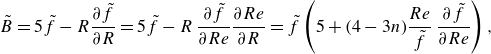 \begin{equation} \tilde {B} = 5\tilde {f}-R\frac {\partial {\tilde {f}}}{\partial {R}} = 5\tilde {f}-R\,\frac {\partial {\tilde {f}}}{\partial {Re}}\frac {\partial {Re}}{\partial {R}} = \tilde {f}\left (5 +(4-3n)\frac {Re}{\tilde {f}} \,\frac {\partial {\tilde {f}}}{\partial {Re}}\right ), \end{equation}
where differentiation of (2.4) provides ${\partial {Re}}/{\partial {R}} = -(4-3n) {Re}/{R}$
. Therefore, knowing
${\partial {Re}}/{\partial {R}} = -(4-3n) {Re}/{R}$
. Therefore, knowing $\tilde {\tau }_0$
,
$\tilde {\tau }_0$
, $\tilde {Q}$
,
$\tilde {Q}$
, $\tilde {\varepsilon }$
and
$\tilde {\varepsilon }$
and $n$
, one can determine the optimal
$n$
, one can determine the optimal $Re$
for a channel.
$Re$
for a channel.
We conclude this section by introducing dimensionless groups that will be used in § 3. The Hedström number $He$
is defined (Swamee & Aggarwal Reference Swamee and Aggarwal2011) and rewritten as follows:
$He$
is defined (Swamee & Aggarwal Reference Swamee and Aggarwal2011) and rewritten as follows:
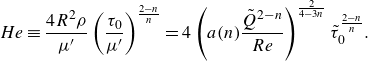 \begin{equation} He \equiv \frac {4R^{2}\rho }{\mu '}\left (\frac {\tau _0}{\mu '}\right )^{\frac {2-n}{n}} =4\left (a(n)\frac {\tilde {Q}^{2-n}}{Re}\right )^{\frac {2}{4-3n}}\tilde {\tau }_0^{\frac {2-n}{n}}. \end{equation}
The relative roughness $\delta$
becomes in the new dimensionless groups
$\delta$
becomes in the new dimensionless groups
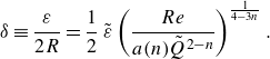 \begin{equation} \delta \equiv \frac {\varepsilon }{2R} =\frac {1}{2}\, \tilde {\varepsilon } \left ( \frac {Re}{a(n) \tilde {Q}^{2-n}}\right )^{\frac {1}{4-3n}}. \end{equation}
Characteristic for a yield-stress fluid is the formation of a plug in the centre of the channel, where the local shear stress $\tau _{rz}$
does not exceed the yield stress
$\tau _{rz}$
does not exceed the yield stress $\tau _0$
. The associated plug radius
$\tau _0$
. The associated plug radius $R_p$
is characterised by
$R_p$
is characterised by
 \begin{equation} R_p \equiv \frac {2\tau _0}{\dfrac {\Delta p}{L}}. \end{equation}
Non-dimensionalisation of the plug radius yields the dimensionless plug radius $\phi$
, which often appears in descriptions for
$\phi$
, which often appears in descriptions for $f$
in the case of yield-stress fluids
$f$
in the case of yield-stress fluids
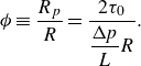 \begin{equation} \phi \equiv \frac {R_p}{R} = \frac {2\tau _0}{\dfrac {\Delta p}{L}R}. \end{equation}
By definition, $\phi$
can also be expressed in terms of the Reynolds and Hedström number and in the new dimensionless groups
$\phi$
can also be expressed in terms of the Reynolds and Hedström number and in the new dimensionless groups
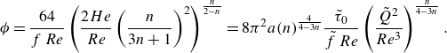 \begin{equation} \phi = \frac {64}{f\, Re}\left (\frac {2He}{Re}\left (\frac {n}{3n+1}\right )^{2}\right )^{\frac {n}{2-n}} = 8\pi ^{2} a(n)^{\frac {4}{4-3n}}\frac {\tilde {\tau }_0}{\tilde {f}\, Re}\left (\frac {\tilde {Q}^{2}}{Re^{3}}\right )^{\frac {n}{4-3n}}. \end{equation}
Up to here, no assumptions are made with respect to the flow type.
3. Network optimisation for different flow regimes and fluid models
The following flow regimes and fluid models are discussed in subsections:
-
§ 3.1 Laminar flow of a Newtonian and non-Newtonian fluids.
-
§ 3.2 Turbulent flow of Newtonian fluids, rough and smooth channels.
-
§ 3.3 Turbulent flow of non-Newtonian fluids, smooth channel, for power-law (§ 3.3.1) and Herschel–Bulkley fluids (§ 3.3.2).
For each fluid model, we will obtain expressions for $\tilde {f}$
, and thereafter for
$\tilde {f}$
, and thereafter for $\tilde {B}$
, which via (2.12) provides the optimal Reynolds number and therefore the optimal radius
$\tilde {B}$
, which via (2.12) provides the optimal Reynolds number and therefore the optimal radius $R$
for each channel via (2.4) and (2.9) . As many expressions for
$R$
for each channel via (2.4) and (2.9) . As many expressions for $\tilde {f}$
and
$\tilde {f}$
and $\tilde {B}$
are implicit, finding an optimal channel radius analytically is often impossible. Therefore, we also provide these results in the form of contour plots for the optimisation condition for
$\tilde {B}$
are implicit, finding an optimal channel radius analytically is often impossible. Therefore, we also provide these results in the form of contour plots for the optimisation condition for $Re$
as a function of
$Re$
as a function of $\tilde {Q}$
and
$\tilde {Q}$
and $\tilde {\tau }_0$
,
$\tilde {\tau }_0$
, $\tilde {\varepsilon }$
or
$\tilde {\varepsilon }$
or $n$
.
$n$
.
3.1. Laminar flow of Newtonian and non-Newtonian fluids
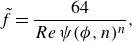
For laminar flow through a circular channel results in the friction factor (Smink et al. Reference Smink, Venner, Visser and Hagmeijer2023)
 \begin{equation} \tilde {f} =\frac {64}{Re \,\psi (\phi, n)^n}, \end{equation}
where $\psi$
is a dimensionless flow rate that ranges from 0 to 1. For laminar flow, the friction factor is often considered to be independent of the channel wall roughness, but this is only true for
$\psi$
is a dimensionless flow rate that ranges from 0 to 1. For laminar flow, the friction factor is often considered to be independent of the channel wall roughness, but this is only true for $\delta \lt 0.01$
. When the roughness becomes of the order of the channel size, then the resulting constricted diameter amplifies the friction factor (Liu, Li & Smits Reference Liu, Li and Smits2019). In this section, it is assumed that the relative channel wall roughness is sufficiently small (
$\delta \lt 0.01$
. When the roughness becomes of the order of the channel size, then the resulting constricted diameter amplifies the friction factor (Liu, Li & Smits Reference Liu, Li and Smits2019). In this section, it is assumed that the relative channel wall roughness is sufficiently small ( $\delta \lt 0.01$
), such that the influence of the wall roughness on the friction factor is negligible. For a Herschel–Bulkley fluid,
$\delta \lt 0.01$
), such that the influence of the wall roughness on the friction factor is negligible. For a Herschel–Bulkley fluid, $\psi$
is computed by integration of the velocity field over the channel’s cross-section as (Herschel & Bulkley Reference Herschel and Bulkley1926; Chilton & Stainsby Reference Chilton and Stainsby1998; Smink et al. Reference Smink, Venner, Visser and Hagmeijer2023)
$\psi$
is computed by integration of the velocity field over the channel’s cross-section as (Herschel & Bulkley Reference Herschel and Bulkley1926; Chilton & Stainsby Reference Chilton and Stainsby1998; Smink et al. Reference Smink, Venner, Visser and Hagmeijer2023)
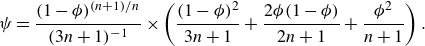 \begin{equation} \psi = \frac {(1-\phi )^{(n+1)/n}}{(3n+1)^{-1}} \times \left ( \frac {(1-\phi )^2}{3n+1}+\frac {2\phi (1-\phi )}{2n+1}+\frac {\phi ^2}{n+1}\right ). \end{equation}
For Bingham fluids ( $n=1$
),
$n=1$
), $\psi$
reduces to (Reiner Reference Reiner1926; Smink et al. Reference Smink, Venner, Visser and Hagmeijer2023)
$\psi$
reduces to (Reiner Reference Reiner1926; Smink et al. Reference Smink, Venner, Visser and Hagmeijer2023)
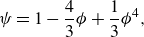 \begin{equation} \psi = 1-\frac {4}{3}\phi +\frac {1}{3}\phi ^4, \end{equation}
and for the case of $\tau _0=0$
(Newtonian and power-law fluids,
$\tau _0=0$
(Newtonian and power-law fluids, $\phi =0$
),
$\phi =0$
), $\psi$
further reduces to 1.
$\psi$
further reduces to 1.
Calculation of the optimisation condition results in the following expression for $\tilde {B}$
:
$\tilde {B}$
:
 \begin{equation} \tilde {B} = \tilde {f}J(\phi, n), \end{equation}
where the function $J(\phi, n)$
is defined as
$J(\phi, n)$
is defined as
 \begin{equation} J\equiv 1+\frac {3n}{1-\dfrac {n\phi }{\psi }\dfrac {\partial {\psi }}{\partial {\phi }}}. \end{equation}
For a Herschel–Bulkley fluid, substitution of $\psi$
from (3.2) into (3.5) results in the following expression for
$\psi$
from (3.2) into (3.5) results in the following expression for $J$
:
$J$
:
 \begin{equation} J = \frac {3n+1}{\dfrac {6n^3}{(2n+1)(n+1)}\phi ^3+\dfrac {6n^2}{(2n+1)(n+1)}\phi ^2+\dfrac {3n}{2n+1}\phi +1}. \end{equation}
For Bingham fluids ( $n=1$
), the expression for
$n=1$
), the expression for $J$
reduces to
$J$
reduces to
 \begin{equation} J = \frac {4}{\phi ^3+\phi ^2+\phi +1}, \end{equation}
and for non-yield fluids ( $\phi =0$
), it reduces to
$\phi =0$
), it reduces to $J=3n+1$
. Finally, for the yield limit (
$J=3n+1$
. Finally, for the yield limit ( $\phi =1$
), one obtains
$\phi =1$
), one obtains $J=1$
.
$J=1$
.
Substitution of $\tilde {B}$
into (2.12) reduces the optimisation condition to
$\tilde {B}$
into (2.12) reduces the optimisation condition to
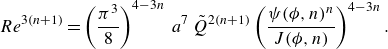 \begin{equation} Re^{3(n+1)}=\left (\frac {\pi ^3}{8}\right )^{4-3n}\, a^7\, \tilde {Q}^{2(n+1)} \left (\frac {\psi (\phi, n)^n}{J(\phi, n)}\right )^{4-3n}. \end{equation}
Together with (2.18) and (3.1), $Re$
is then explicitly solved for given
$Re$
is then explicitly solved for given $\tilde {Q}$
,
$\tilde {Q}$
, $\tilde {\tau }_0$
and
$\tilde {\tau }_0$
and $n$
, providing the optimal radius via (2.4) and (2.9). Figures 8(a)–8(c) in Appendix E present a contour plot for the optimal
$n$
, providing the optimal radius via (2.4) and (2.9). Figures 8(a)–8(c) in Appendix E present a contour plot for the optimal $Re$
as function of
$Re$
as function of $\tilde {Q}$
and
$\tilde {Q}$
and $\tilde {\tau }_0$
for different values of
$\tilde {\tau }_0$
for different values of $n$
. Note that the number of parameters can be reduced even further, by combining
$n$
. Note that the number of parameters can be reduced even further, by combining $\tilde {Q}$
and
$\tilde {Q}$
and $Re$
, to a parameter which is only a function of given
$Re$
, to a parameter which is only a function of given $\tilde {\tau }_0$
and
$\tilde {\tau }_0$
and $n$
. Then the optimisation condition becomes (Smink et al. Reference Smink, Venner, Visser and Hagmeijer2023)
$n$
. Then the optimisation condition becomes (Smink et al. Reference Smink, Venner, Visser and Hagmeijer2023)
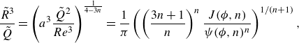 \begin{equation} \frac {\tilde {R}^3}{\tilde {Q}} =\left ( a^3\frac {\tilde {Q}^2}{Re^3}\right )^{\frac {1}{4-3n}}= \frac {1}{\pi }\left (\left (\frac {3n+1}{n}\right )^n \frac {J(\phi, n)}{\psi (\phi, n)^n}\right )^{1/(n+1)}, \end{equation}
where the right-hand side is constant for an optimised network. Plotting ${\tilde {R}^3}/{\tilde {Q}}$
as function of
${\tilde {R}^3}/{\tilde {Q}}$
as function of $\tilde {\tau }_0$
and
$\tilde {\tau }_0$
and $n$
gives the contour plot in figure 8(d) in Appendix E. This figure can be made for laminar flows because
$n$
gives the contour plot in figure 8(d) in Appendix E. This figure can be made for laminar flows because $\tilde {R}^3/\tilde {Q}$
is constant over the entire network, which is highly useful for design of optimised branched fluidic networks, as only one optimisation condition has to be calculated.
$\tilde {R}^3/\tilde {Q}$
is constant over the entire network, which is highly useful for design of optimised branched fluidic networks, as only one optimisation condition has to be calculated.
3.2. Turbulent flow of Newtonian fluid, rough and smooth channel
We now demonstrate that the proposed optimisation method is universal if the friction factor is known, by optimising networks for diverse turbulent flow regimes. For turbulent flow of a Newtonian fluid, the Colebrook-White equation (Colebrook Reference Colebrook1939) describes the friction factor for both low- and high-turbulent flow ( $Re = [Re_{crit},\infty \rangle$
) in hydraulically smooth and rough pipes using the following implicit equation:
$Re = [Re_{crit},\infty \rangle$
) in hydraulically smooth and rough pipes using the following implicit equation:
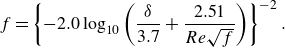 \begin{equation} f = \left \{-2.0\log _{10}\left (\frac {\delta }{3.7}+\frac {2.51}{Re\sqrt {f}}\right )\right \}^{-2}. \end{equation}
Equation (3.10) underlies the well-known Moody diagram (Moody Reference Moody1944) as shown in figure 2(b). Rewriting (3.10) in terms of the dimensionless numbers gives
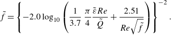 \begin{equation} \tilde {f} = \left \{-2.0\log _{10}\left (\frac {1}{3.7}\,\frac {\pi }{4}\frac {\tilde {\varepsilon }Re}{\tilde {Q}}+\frac {2.51}{Re\sqrt {\tilde {f}}}\right )\right \}^{-2}. \end{equation}
Differentiation to $Re$
gives
$Re$
gives
 \begin{equation} \frac {\partial {\tilde {f}}}{\partial {Re}} = -\frac {\tilde {f}}{Re}\frac {2\left (\dfrac {1}{3.7}\,\dfrac {\pi }{4}\dfrac {\tilde {\varepsilon }Re}{\tilde {Q}}-\dfrac {2.51}{Re\sqrt {\tilde {f}}}\right )}{\left (\dfrac {1}{3.7}\,\dfrac {\pi }{4}\dfrac {\tilde {\varepsilon }Re}{\tilde {Q}}+\dfrac {2.51}{Re\sqrt {\tilde {f}}}\right )\ln \left (\dfrac {1}{3.7}\,\dfrac {\pi }{4}\dfrac {\tilde {\varepsilon }Re}{\tilde {Q}}+\dfrac {2.51}{Re\sqrt {\tilde {f}}}\right )-\dfrac {2.51}{Re\sqrt {\tilde {f}}}}, \end{equation}
resulting in
 \begin{equation} \tilde {B} = \tilde {f}\left (5-\frac {2\left (\dfrac {1}{3.7}\,\dfrac {\pi }{4}\dfrac {\tilde {\varepsilon }Re}{\tilde {Q}}-\dfrac {2.51}{Re\sqrt {\tilde {f}}}\right )}{\left (\dfrac {1}{3.7}\,\dfrac {\pi }{4}\dfrac {\tilde {\varepsilon }Re}{\tilde {Q}}+\dfrac {2.51}{Re\sqrt {\tilde {f}}}\right )\ln \left (\dfrac {1}{3.7}\,\dfrac {\pi }{4}\dfrac {\tilde {\varepsilon }Re}{\tilde {Q}}+\dfrac {2.51}{Re\sqrt {\tilde {f}}}\right )-\dfrac {2.51}{Re\sqrt {\tilde {f}}}}\right ). \end{equation}
Substituting $\tilde {B}$
into (2.12) enables implicit solving
$\tilde {B}$
into (2.12) enables implicit solving $Re$
for given
$Re$
for given $\tilde {Q}$
. Contour plots of the optimal
$\tilde {Q}$
. Contour plots of the optimal $Re$
as function
$Re$
as function $\tilde {Q}$
and
$\tilde {Q}$
and $\tilde {\varepsilon }$
are presented in figure 3(a). Limit cases of the Colebrook–White equation include complete turbulence (for which Von Kármán’s formula applies), turbulence in smooth channels and low-Reynolds-number turbulence in smooth channels (e.g. Blasius’ formula). Expressions of the optimal channel radius for these cases are derived in Appendix B.
$\tilde {\varepsilon }$
are presented in figure 3(a). Limit cases of the Colebrook–White equation include complete turbulence (for which Von Kármán’s formula applies), turbulence in smooth channels and low-Reynolds-number turbulence in smooth channels (e.g. Blasius’ formula). Expressions of the optimal channel radius for these cases are derived in Appendix B.
Figure 3. Optimal $Re$
for different fluid models. The colour-scale contour lines represent the Reynolds numbers
$Re$
for different fluid models. The colour-scale contour lines represent the Reynolds numbers $2\times 10^{x}$
,
$2\times 10^{x}$
, $3\times 10^{x}$
, …
$3\times 10^{x}$
, … $9\times 10^{x}$
with decreasing brightness. (a) Contour plot of the optimal
$9\times 10^{x}$
with decreasing brightness. (a) Contour plot of the optimal $Re$
as function of
$Re$
as function of $\tilde {Q}$
and
$\tilde {Q}$
and $\tilde {\varepsilon }$
for a Newtonian fluid in a rough-wall channel. (b) Contour plot of the optimal
$\tilde {\varepsilon }$
for a Newtonian fluid in a rough-wall channel. (b) Contour plot of the optimal $Re$
as function of
$Re$
as function of $\tilde {Q}$
and
$\tilde {Q}$
and $n$
for a power-law fluid in a smooth-wall channel. (c) Contour plot of the optimal
$n$
for a power-law fluid in a smooth-wall channel. (c) Contour plot of the optimal $Re$
as function of
$Re$
as function of $\tilde {Q}$
and
$\tilde {Q}$
and $\tilde {\varepsilon }$
for a Herschel–Bulkley fluid (
$\tilde {\varepsilon }$
for a Herschel–Bulkley fluid ( $n=1$
) in a smooth-wall channel.
$n=1$
) in a smooth-wall channel.
3.3. Turbulent flow of non-Newtonian fluids, smooth channel
3.3.1. Power-law fluid
Turbulent pipe flow of non-Newtonian power-law fluids at low Reynolds numbers in a smooth circular channel ( $\varepsilon \rightarrow 0$
) was analysed by, amongst others, Dodge and Metzner (Dodge & Metzner Reference Dodge and Metzner1959). They modified the Von Kármán equation for turbulent Newtonian pipe flow, resulting in an implicit relation for the Darcy friction factor
$\varepsilon \rightarrow 0$
) was analysed by, amongst others, Dodge and Metzner (Dodge & Metzner Reference Dodge and Metzner1959). They modified the Von Kármán equation for turbulent Newtonian pipe flow, resulting in an implicit relation for the Darcy friction factor $f$
$f$
 \begin{equation} \frac {2}{\sqrt {f}}=\frac {4}{n^{0.75}}\log _{10}\left (Re\left (\frac {f}{4}\right )^{1-n/2}\right )-\frac {0.4}{n^{1.2}} .\end{equation}
The value of $f$
is shown as a function of
$f$
is shown as a function of $Re$
and
$Re$
and $n$
in figure 2(c).
$n$
in figure 2(c).
Implicit differentiation of $\tilde {f}$
to
$\tilde {f}$
to $Re$
gives
$Re$
gives
 \begin{equation} \frac {\partial {\tilde {f}}}{\partial {Re}} = -\frac {\tilde {f}}{Re}\left ( \frac {n^{0.75}\ln 10}{4\sqrt {\tilde {f}}}+1-\frac {n}{2} \right )^{-1}, \end{equation}
resulting in
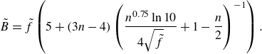 \begin{equation} \tilde {B} = \tilde {f}\left (5+(3n-4)\left ( \frac {n^{0.75}\ln 10}{4\sqrt {\tilde {f}}}+1-\frac {n}{2} \right )^{-1}\right ). \end{equation}
Here, $\tilde {B}$
is still a function of
$\tilde {B}$
is still a function of $\tilde {f}$
, which is in turn an implicit function of
$\tilde {f}$
, which is in turn an implicit function of $Re$
governed by (3.14). Therefore,
$Re$
governed by (3.14). Therefore, $\tilde {B}$
is governed by
$\tilde {B}$
is governed by $Re$
and the flow index
$Re$
and the flow index $n$
. Consequently, with this expression for
$n$
. Consequently, with this expression for $\tilde {B}$
, the optimal value of
$\tilde {B}$
, the optimal value of $Re$
in a channel can be calculated as function of
$Re$
in a channel can be calculated as function of $\tilde {Q}$
and
$\tilde {Q}$
and $n$
. A contour plot for the optimal Reynolds number in a channel is given in figure 3(b).
$n$
. A contour plot for the optimal Reynolds number in a channel is given in figure 3(b).
3.3.2. Herschel–Bulkley fluid
For a turbulent flow of a Herschel–Bulkley fluid in a smooth circular channel ( $\varepsilon \rightarrow 0$
), Torrance (Garcia & Steffe Reference Garcia and Steffe1986) developed a relationship for the friction factor. This relation for the Darcy friction factor is given by
$\varepsilon \rightarrow 0$
), Torrance (Garcia & Steffe Reference Garcia and Steffe1986) developed a relationship for the friction factor. This relation for the Darcy friction factor is given by
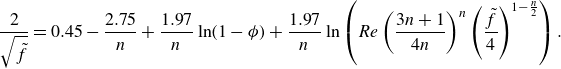 \begin{equation} \frac {2}{\sqrt {\tilde {f}}}=0.45-\frac {2.75}{n}+\frac {1.97}{n}\ln (1-\phi ) +\frac {1.97}{n}\ln \left (Re\left (\frac {3n+1}{4n}\right )^n \left (\frac {\tilde {f}}{4}\right )^{1-\frac {n}{2}}\right ). \end{equation}
Here, $\phi$
as given in (2.18) is used in the calculations. Figure 2(d) shows
$\phi$
as given in (2.18) is used in the calculations. Figure 2(d) shows $f$
as function of
$f$
as function of $Re$
for
$Re$
for $n=1.0$
and a range of values of
$n=1.0$
and a range of values of $\tilde {\tau }_0$
.The
$\tilde {\tau }_0$
.The $f$
-
$f$
- $Re$
plots for other values of
$Re$
plots for other values of $n$
are presented in figure 7 in Appendix E.
$n$
are presented in figure 7 in Appendix E.
Implicit differentiation of $\tilde {f}$
to
$\tilde {f}$
to $Re$
leads to
$Re$
leads to
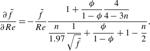 \begin{equation} \frac {\partial \tilde {f}}{\partial Re} = -\frac {\tilde {f}}{Re}\frac {1+\dfrac {\phi }{1-\phi }\dfrac {4}{4-3n}}{\dfrac {n}{1.97}\dfrac {1}{\sqrt {\tilde {f}}}+\dfrac {\phi }{1-\phi }+1-\dfrac {n}{2}}, \end{equation}
giving an expression for $\tilde {B}$
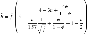 \begin{equation} \tilde {B} = \tilde {f}\left (5-\frac {4-3n+\dfrac {4\phi }{1-\phi }}{\dfrac {n}{1.97}\dfrac {1}{\sqrt {\tilde {f}}}+\dfrac {\phi }{1-\phi }+1-\dfrac {n}{2}}\right ). \end{equation}
Contour plots for the optimal Reynolds number in a channel as function of $\tilde {\tau }_0$
and
$\tilde {\tau }_0$
and $\tilde {Q}$
are given for
$\tilde {Q}$
are given for $n=1.0$
in figure 3(c) and the results for
$n=1.0$
in figure 3(c) and the results for $n=0.5$
and
$n=0.5$
and $n=1.5$
are provided in figure 9 in Appendix E. An additional fluid model covering laminar and turbulent flow of a Bingham fluid is presented in Appendix C.
$n=1.5$
are provided in figure 9 in Appendix E. An additional fluid model covering laminar and turbulent flow of a Bingham fluid is presented in Appendix C.
4. Scaling of the channel radii
In the literature, many attempts have been made to find the proportionality between the flow rate $Q$
and the channel radius
$Q$
and the channel radius $R$
for optimised networks, in the form of (1.1) (Uylings Reference Uylings1977; Sherman Reference Sherman1981; Woldenberg & Horsfield Reference Woldenberg and Horsfield1986; Williams et al. Reference Williams, Trask, Weaver and Bond2008; Kou et al. Reference Kou, Chen, Zhou, Lu, Wu and Fan2014). In the optimisation method of the present study, only
$R$
for optimised networks, in the form of (1.1) (Uylings Reference Uylings1977; Sherman Reference Sherman1981; Woldenberg & Horsfield Reference Woldenberg and Horsfield1986; Williams et al. Reference Williams, Trask, Weaver and Bond2008; Kou et al. Reference Kou, Chen, Zhou, Lu, Wu and Fan2014). In the optimisation method of the present study, only $Re$
and
$Re$
and $\tilde {Q}$
contain parameters involving
$\tilde {Q}$
contain parameters involving $R$
and
$R$
and $Q$
, while
$Q$
, while $\tilde {\tau }_0$
,
$\tilde {\tau }_0$
, $\tilde {\varepsilon }$
and
$\tilde {\varepsilon }$
and $n$
are independent of
$n$
are independent of $R$
and
$R$
and $Q$
. Therefore, when knowing the proportionality between
$Q$
. Therefore, when knowing the proportionality between $\tilde {Q}$
and
$\tilde {Q}$
and $Re$
,
$Re$
, $x$
can be calculated analytically. However, this only holds if
$x$
can be calculated analytically. However, this only holds if $\tilde {B} \propto Re^{c_1}\tilde {Q}^{c_2}$
, which is only true for relatively simple descriptions of
$\tilde {B} \propto Re^{c_1}\tilde {Q}^{c_2}$
, which is only true for relatively simple descriptions of $f$
applicable to laminar flows or limit cases of the turbulent regime (e.g. Blasius’ formula, Appendix B.3). Therefore, in the following,
$f$
applicable to laminar flows or limit cases of the turbulent regime (e.g. Blasius’ formula, Appendix B.3). Therefore, in the following, $x$
will be calculated by locally approximating
$x$
will be calculated by locally approximating $\tilde {B}$
by a power function via
$\tilde {B}$
by a power function via
 \begin{equation} x = \displaystyle\frac {R}{Q}\displaystyle\frac {\partial Q}{\partial R}= \displaystyle\frac {(4-3n)\dfrac {Re}{\tilde {Q}}\dfrac {\partial {\tilde {Q}}}{\partial {Re}}}{(2-n)\dfrac {Re}{\tilde {Q}}\dfrac {\partial {\tilde {Q}}}{\partial {Re}}-1}. \end{equation}
By calculating the fluid-model-specific $({Re}/{\tilde {Q}})\, {\partial {\tilde {Q}}}/{\partial {Re}}$
, one obtains
$({Re}/{\tilde {Q}})\, {\partial {\tilde {Q}}}/{\partial {Re}}$
, one obtains $x$
in the relevant (
$x$
in the relevant ( $Re,\tilde {\tau }_0,\tilde {\varepsilon },n$
)-space, as shown in figure 4 for the different fluid models (the underlying equations are shown in Appendix D). Known limit cases are shown in black; all coloured results are new. For laminar flow of all treated fluid models,
$Re,\tilde {\tau }_0,\tilde {\varepsilon },n$
)-space, as shown in figure 4 for the different fluid models (the underlying equations are shown in Appendix D). Known limit cases are shown in black; all coloured results are new. For laminar flow of all treated fluid models, $x$
becomes 3, as expected (Murray Reference Murray1926b
; Smink et al. Reference Smink, Venner, Visser and Hagmeijer2023) For networks that span ranges of
$x$
becomes 3, as expected (Murray Reference Murray1926b
; Smink et al. Reference Smink, Venner, Visser and Hagmeijer2023) For networks that span ranges of $Re$
for which
$Re$
for which $x$
is (almost) constant, the value of
$x$
is (almost) constant, the value of $x$
is readily used to scale all channels in the network if one optimal diameter is known, using
$x$
is readily used to scale all channels in the network if one optimal diameter is known, using $Q\propto R^{x}$
.
$Q\propto R^{x}$
.
Figure 4. Plot of $x$
(4.1) as function of
$x$
(4.1) as function of $Re$
for the different fluid models as discussed in § 3. The dashed lines for
$Re$
for the different fluid models as discussed in § 3. The dashed lines for $x=3$
and
$x=3$
and $x=7/3$
show the expected limit cases for laminar flow and high-turbulent flow, respectively (Uylings Reference Uylings1977). (a) Turbulent flow of Newtonian fluids, described by Colebrook–White (
$x=7/3$
show the expected limit cases for laminar flow and high-turbulent flow, respectively (Uylings Reference Uylings1977). (a) Turbulent flow of Newtonian fluids, described by Colebrook–White ( $\tilde {\varepsilon } \in [10^{-5},10^{1},10^{2},10^{3},10^{4},10^{5}]$
), Blasius’ formula (B12) and an empirical relation (B14). The blue
$\tilde {\varepsilon } \in [10^{-5},10^{1},10^{2},10^{3},10^{4},10^{5}]$
), Blasius’ formula (B12) and an empirical relation (B14). The blue $\times$
-symbols correspond with the optimised channels in figure 1(e), showing that the values for
$\times$
-symbols correspond with the optimised channels in figure 1(e), showing that the values for $x$
change significantly for that network. (b) Plot of
$x$
change significantly for that network. (b) Plot of $x$
as function of
$x$
as function of $Re$
for turbulent flow of a Newtonian fluid in a hydraulically smooth channel, described by (3.10) for the limit of
$Re$
for turbulent flow of a Newtonian fluid in a hydraulically smooth channel, described by (3.10) for the limit of $\tilde {\varepsilon }=0$
. For optimised networks, high-
$\tilde {\varepsilon }=0$
. For optimised networks, high- $Re$
turbulent flow in smooth channels will for realistic
$Re$
turbulent flow in smooth channels will for realistic $Re$
never reach
$Re$
never reach $x=7/3$
. (c) Plot of
$x=7/3$
. (c) Plot of $x$
as function of
$x$
as function of $\delta = \varepsilon /2R$
for high-
$\delta = \varepsilon /2R$
for high- $Re$
turbulent flow of a Newtonian fluid in a rough channel, described by (B1). For optimised networks, high-
$Re$
turbulent flow of a Newtonian fluid in a rough channel, described by (B1). For optimised networks, high- $Re$
turbulent flow in channels with finite roughness will never reach
$Re$
turbulent flow in channels with finite roughness will never reach $x=7/3$
. (d) Turbulent flow of a power-law fluid (Metzner & Dodge) (
$x=7/3$
. (d) Turbulent flow of a power-law fluid (Metzner & Dodge) ( $n\in [0.2,0.4,1.0,1.4,1.8]$
). (e) Turbulent flow of a Herschel–Bulkley fluid (Torrance) (
$n\in [0.2,0.4,1.0,1.4,1.8]$
). (e) Turbulent flow of a Herschel–Bulkley fluid (Torrance) ( $\tilde {\tau }_0 \in [0.1,0.25,1,2.5,10,25]$
with
$\tilde {\tau }_0 \in [0.1,0.25,1,2.5,10,25]$
with $n= 1.0$
). Plots for
$n= 1.0$
). Plots for $n=0.5$
and
$n=0.5$
and $n=1.5$
are presented in figure 10 in Appendix E.
$n=1.5$
are presented in figure 10 in Appendix E.
For a Newtonian fluid (figure 4
a), at the transition from laminar to turbulent flow, $x$
drops quickly from 3 to around 2.5 for hydraulically smooth channels. We find that the low-
$x$
drops quickly from 3 to around 2.5 for hydraulically smooth channels. We find that the low- $Re$
approximations (Blasius,
$Re$
approximations (Blasius, $x=27/11$
, and an empirical relation,
$x=27/11$
, and an empirical relation, $x=17/7$
(Kou et al. Reference Kou, Chen, Zhou, Lu, Wu and Fan2014)) correspond to the average value of
$x=17/7$
(Kou et al. Reference Kou, Chen, Zhou, Lu, Wu and Fan2014)) correspond to the average value of $x$
over their applicable
$x$
over their applicable $Re$
-range of the Colebrook–White equation for a smooth channel. Although these approximations and the resulting values of
$Re$
-range of the Colebrook–White equation for a smooth channel. Although these approximations and the resulting values of $x$
are valuable for networks that span a limited range of the Reynolds number, the network shown in figure 1(e) represents a case where
$x$
are valuable for networks that span a limited range of the Reynolds number, the network shown in figure 1(e) represents a case where $x$
is not applicable for determination of the optimal channel radii. Here, the optimal network partly corresponds to laminar flow and partly to turbulent flow. As these regimes result in strongly different values of
$x$
is not applicable for determination of the optimal channel radii. Here, the optimal network partly corresponds to laminar flow and partly to turbulent flow. As these regimes result in strongly different values of $x$
, as shown by the markers (
$x$
, as shown by the markers ( $\times$
) in figure 4(a), the so-called Murray’s law (Sherman Reference Sherman1981; Stephenson & Lockerby Reference Stephenson and Lockerby2016) (
$\times$
) in figure 4(a), the so-called Murray’s law (Sherman Reference Sherman1981; Stephenson & Lockerby Reference Stephenson and Lockerby2016) ( $R_0^{x} = \sum _i R_i^{x}$
, for one branching point) will not hold. Therefore, the optimal radius of each channel must be calculated individually.
$R_0^{x} = \sum _i R_i^{x}$
, for one branching point) will not hold. Therefore, the optimal radius of each channel must be calculated individually.
Figure 4(a) also shows that $x$
increases for increasing wall roughness. The lines are clipped for
$x$
increases for increasing wall roughness. The lines are clipped for $\delta = 0.1$
, corresponding to
$\delta = 0.1$
, corresponding to $x \approx 2.71$
. Analysing the Colebrook–White equation for the smooth-channel limit (
$x \approx 2.71$
. Analysing the Colebrook–White equation for the smooth-channel limit ( $\tilde {\varepsilon }=0$
) shows that, for extremely large
$\tilde {\varepsilon }=0$
) shows that, for extremely large $Re$
,
$Re$
, $x$
will indeed approach
$x$
will indeed approach $x=7/3$
, as shown in figure 4(b). The high-
$x=7/3$
, as shown in figure 4(b). The high- $Re$
limit for non-zero roughness, however (figure 4(c),
$Re$
limit for non-zero roughness, however (figure 4(c), $\tilde {\varepsilon }= \text{const.}$
), shows that
$\tilde {\varepsilon }= \text{const.}$
), shows that $x=7/3$
will never be reached if a finite value of
$x=7/3$
will never be reached if a finite value of $\delta$
is included in the optimisation process.
$\delta$
is included in the optimisation process.
When using the Colebrook–White equation, one has to make an assumption about the wall roughness. Figure 4(a) shows the results for a fixed dimensionless absolute roughness $\tilde {\varepsilon }$
. One can also choose to fix the relative wall roughness
$\tilde {\varepsilon }$
. One can also choose to fix the relative wall roughness $\delta$
, which has often been an implicit assumption in previous works (Uylings Reference Uylings1977; Bejan et al. Reference Bejan, Rocha L.A. and Lorente2000; Kou et al. Reference Kou, Chen, Zhou, Lu, Wu and Fan2014; Stephenson & Lockerby Reference Stephenson and Lockerby2016; Zhou et al. Reference Zhou2024). Then
$\delta$
, which has often been an implicit assumption in previous works (Uylings Reference Uylings1977; Bejan et al. Reference Bejan, Rocha L.A. and Lorente2000; Kou et al. Reference Kou, Chen, Zhou, Lu, Wu and Fan2014; Stephenson & Lockerby Reference Stephenson and Lockerby2016; Zhou et al. Reference Zhou2024). Then $\delta$
is excluded from the optimisation procedure. Only in this case, it holds for complete turbulence in rough-wall channels that
$\delta$
is excluded from the optimisation procedure. Only in this case, it holds for complete turbulence in rough-wall channels that $x=7/3$
(figure 4
c,
$x=7/3$
(figure 4
c, $\delta = \text{const.}$
). The assumption of a fixed
$\delta = \text{const.}$
). The assumption of a fixed $\delta$
requires that the absolute roughness
$\delta$
requires that the absolute roughness $\varepsilon$
is proportional to the optimised channel radius for every channel in the network. However, many networks consist of a given wall material with uniform absolute roughness
$\varepsilon$
is proportional to the optimised channel radius for every channel in the network. However, many networks consist of a given wall material with uniform absolute roughness $\varepsilon$
. Even when there is a changing absolute roughness in the network, the choice for the use of
$\varepsilon$
. Even when there is a changing absolute roughness in the network, the choice for the use of $\tilde {\varepsilon }$
is preferred and then the graphical approach (figure 3
a) can be used for optimisation of the channel radii.
$\tilde {\varepsilon }$
is preferred and then the graphical approach (figure 3
a) can be used for optimisation of the channel radii.
Figure 4(d) shows $x$
for turbulent flow of a power-law fluid in smooth channels. The behaviour of
$x$
for turbulent flow of a power-law fluid in smooth channels. The behaviour of $x$
is similar to that of a Newtonian fluid in a smooth channel, but increases slightly with increasing
$x$
is similar to that of a Newtonian fluid in a smooth channel, but increases slightly with increasing $n$
. Figure 4(e) shows the results for a Herschel–Bulkley fluid (
$n$
. Figure 4(e) shows the results for a Herschel–Bulkley fluid ( $n=1.0$
), which appears to have a complete transition from
$n=1.0$
), which appears to have a complete transition from $x=3$
to
$x=3$
to $x\rightarrow 7/3$
, with a remarkable bump in the transition, which is related to the sharp corner around
$x\rightarrow 7/3$
, with a remarkable bump in the transition, which is related to the sharp corner around $10^1\lt \tilde {\tau }_0\lt 10^2$
as observed in the optimisation plot (figure 3
c). The transition occurs at larger
$10^1\lt \tilde {\tau }_0\lt 10^2$
as observed in the optimisation plot (figure 3
c). The transition occurs at larger $Re$
for increasing
$Re$
for increasing $\tilde {\tau }_0$
, and for large
$\tilde {\tau }_0$
, and for large $Re$
, all lines converge. Results for
$Re$
, all lines converge. Results for $n=0.5$
and
$n=0.5$
and $n=1.5$
are presented in figure 10 in Appendix E.
$n=1.5$
are presented in figure 10 in Appendix E.
The transitional behaviour of $x$
as presented in figure 4 stresses its importance for network optimisation when considering turbulent flow. For domains of
$x$
as presented in figure 4 stresses its importance for network optimisation when considering turbulent flow. For domains of $Re$
where
$Re$
where $x$
is approximately constant, figure 4 enables making a quick estimation of the optimal channel radii within a network. If one channel within a network has been optimised, then the other channels can be optimised using
$x$
is approximately constant, figure 4 enables making a quick estimation of the optimal channel radii within a network. If one channel within a network has been optimised, then the other channels can be optimised using $Q\propto R^{x}$
. For domains of
$Q\propto R^{x}$
. For domains of $Re$
where
$Re$
where $x$
clearly non-constant, the full computations of the equations or the use of the graphical approach of figure 3 is required.
$x$
clearly non-constant, the full computations of the equations or the use of the graphical approach of figure 3 is required.
5. Synthesis: design of an optimised fluidic network
The framework described in §§ 2, 3 and 4 leads to the following approach for optimisation of branched fluidic networks (such as shown in figure 1 e,f):
-
(i) Determine the fluid model and the cost factor $\alpha$
, and calculate
$\tilde {\tau }_0$
,
$\tilde {\varepsilon }$
and
$n$
. Calculate
$\tilde {Q}$
for all the to be optimised channels (§ 2).
$\alpha$
, and calculate
$\tilde {\tau }_0$
,
$\tilde {\varepsilon }$
and
$n$
. Calculate
$\tilde {Q}$
for all the to be optimised channels (§ 2). -
(ii) Determine the optimal radius
$R$
in one channel.-
(a) First, determine the optimal
$Re$
by one of the following options:
-


-
– Read
$Re$
from an optimisation contour plot (e.g. Figure 3
a) for given
$\tilde {Q}$
. -
– Calculate
$\tilde {B}(\tilde {f},Re,\tilde {Q},\tilde {\tau }_0,\tilde {\varepsilon },n)$
via (2.13) and then solve (2.12) for
$Re$
for given
$\tilde {Q}$
.


-
(b) Subsequently, calculate
$R$
from the calculated
$Re$
by using (2.4).


-
(iii) Obtain all channel radii:
-
– By repeating step 2 for each channel, or
-
– by obtaining
$x$
from figure 4 and calculating all channel radii using
$Q\propto R^{x}$
. This option only applies if
$x$
is (almost) constant over the applicable range of
$Re$
.
-
-
(iv) Calculate the optimal location of the branching points (Appendix A.1).


This approach is illustrated by an example of the optimisation of a fluidic network with turbulent flow of a Newtonian fluid in rough-wall channels, presented in Appendix F.
6. Conclusion
A unifying design procedure for optimisation of branched fluidic networks was presented. The optimal channel radius is obtained by minimising the power consumption for maintaining the flow and minimising the volume simultaneously, which is carried out for all channel segments individually. The approach is applicable to every flow configuration for which the Darcy friction factor is available, even for non-power-law or implicit formulations.
Network optimisation was carried out for the parameter space spanned by the Reynolds number (laminar and turbulent flows), the wall roughness and for different rheologies. This parameter space is widely applicable to e.g. heat exchangers or (inertial) microfluidics, but was hardly covered in the literature, as shown in figure 1(a,b). First, the entire optimisation problem is non-dimensionalised in terms of $Re$
,
$Re$
, $\tilde {Q}$
,
$\tilde {Q}$
, $\tilde {\tau }_0$
,
$\tilde {\tau }_0$
, $\tilde {\varepsilon }$
and
$\tilde {\varepsilon }$
and $n$
. For every channel, the optimal Reynolds number and the optimal channel radius are obtained as a function of the dimensionless flow rate
$n$
. For every channel, the optimal Reynolds number and the optimal channel radius are obtained as a function of the dimensionless flow rate $\tilde {Q}$
. To minimise the required mathematical analysis, graphs are presented that readily provide the optimal Reynolds number for every fluid model.
$\tilde {Q}$
. To minimise the required mathematical analysis, graphs are presented that readily provide the optimal Reynolds number for every fluid model.
Subsequently, the value of $x$
in the proportionality
$x$
in the proportionality $Q\propto R^{x}$
was evaluated for the full parameter space of the Reynolds number and channel roughness for different fluid rheologies. The well-known limit values
$Q\propto R^{x}$
was evaluated for the full parameter space of the Reynolds number and channel roughness for different fluid rheologies. The well-known limit values $x=3$
for laminar flow and
$x=3$
for laminar flow and $x=7/3$
for high-
$x=7/3$
for high- $Re$
turbulence were recovered (Uylings Reference Uylings1977; Bejan et al. Reference Bejan, Rocha L.A. and Lorente2000; Kou et al. Reference Kou, Chen, Zhou, Lu, Wu and Fan2014; Stephenson & Lockerby Reference Stephenson and Lockerby2016; Zhou et al. Reference Zhou2024). However, as the latter value is hardly reached in practice, the intermediate values of
$Re$
turbulence were recovered (Uylings Reference Uylings1977; Bejan et al. Reference Bejan, Rocha L.A. and Lorente2000; Kou et al. Reference Kou, Chen, Zhou, Lu, Wu and Fan2014; Stephenson & Lockerby Reference Stephenson and Lockerby2016; Zhou et al. Reference Zhou2024). However, as the latter value is hardly reached in practice, the intermediate values of $x$
were calculated and plotted. This revealed in which case the entire network can be optimised based on one optimal channel radius, and in which case all radii must be optimised individually. Finally, a design procedure of optimised fluidic networks that incorporates all aforementioned elements was presented.
$x$
were calculated and plotted. This revealed in which case the entire network can be optimised based on one optimal channel radius, and in which case all radii must be optimised individually. Finally, a design procedure of optimised fluidic networks that incorporates all aforementioned elements was presented.
Our unifying approach for optimisation of fluidic networks can be extended to other configurations with known friction factors, including non-circular cross-sections, bended pipes, bubbly flows, porous walls (Miguel Reference Miguel2018), porous media (MacDonald et al. Reference MacDonald, Chu, Guilloit and Ng1991) or slip flow (Morini & Spiga Reference Morini and Spiga1998). As such, it enables optimisation of many realistically encountered configurations in nature and engineering.
Acknowledgements
E.A. Bramer, K. Jain and T.G. Vlogman are acknowledged for the helpful discussions.
Funding
This work was supported by the Dutch Research Council (NWO) under OCENW.M20.381.
Declaration of interests
The authors report no conflict of interest.
Appendix A. Details on optimisation of a fluidic branching
A.1 Optimal branching point location
To minimise the power in a network, the location of the branching point $\boldsymbol{x}$
must be chosen. If the channel radii are optimised according to (2.12), this is the same as minimising the total volume within the channels. Differentiation of the total power
$\boldsymbol{x}$
must be chosen. If the channel radii are optimised according to (2.12), this is the same as minimising the total volume within the channels. Differentiation of the total power $P$
(2.1) to
$P$
(2.1) to $\boldsymbol{x}$
results in
$\boldsymbol{x}$
results in
 \begin{equation} \nabla _{\boldsymbol{x}}{P}=\sum _{i=0}^N\left (\left |\frac {\textrm {d}p}{\textrm {d}z}\right |_i Q_i + \alpha \pi R_i^2\right ) \boldsymbol{\nabla } L_i=\textbf {0}, \quad i=0,1,\ldots, N, \end{equation}
where we define
 \begin{equation} \boldsymbol{e}_{i,*}\equiv \left (\boldsymbol{\nabla } L_i\right )_*=\frac {\boldsymbol{x}_*-\boldsymbol{x}_i}{|\boldsymbol{x}_*-\boldsymbol{x}_i|}. \end{equation}
Here, the subscript $i$
indicates the index of the channel, and the subscript
$i$
indicates the index of the channel, and the subscript $*$
indicates an optimised parameter.
$*$
indicates an optimised parameter.
Substituting the optimisation condition for the channel radii (2.12) results in the optimisation condition of the branching point $\boldsymbol{x}=\boldsymbol{x}_*$
(for a full derivation, see Smink et al. (Reference Smink, Venner, Visser and Hagmeijer2023))
$\boldsymbol{x}=\boldsymbol{x}_*$
(for a full derivation, see Smink et al. (Reference Smink, Venner, Visser and Hagmeijer2023))
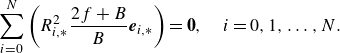 \begin{equation} \sum _{i=0}^N \left (R_{i,*}^2 \frac {2f+B}{B} \boldsymbol{e}_{i,*}\right )=\textbf {0}, \quad i=0,1,\ldots, N. \end{equation}
Alternatively, we can rewrite (A3) in terms of dimensionless numbers
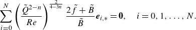 \begin{equation} \sum _{i=0}^N \left (\frac {\tilde {Q}^{2-n}}{Re}\right )^{\frac {2}{4-3n}} \frac {2\tilde {f}+\tilde {B}}{\tilde {B}} \boldsymbol{e}_{i,*}=\textbf {0}, \quad i=0,1,\ldots, N. \end{equation}
Equation (A4) requires the optimal Reynolds number and corresponding $\tilde {f}$
,
$\tilde {f}$
, $\tilde {B}$
and
$\tilde {B}$
and $\tilde {Q}$
for each channel for computation of the optimal branching point location. It is an implicit equation, such that the coordinates of
$\tilde {Q}$
for each channel for computation of the optimal branching point location. It is an implicit equation, such that the coordinates of $\boldsymbol{x}_*$
are solved by simple numerical methods, providing the lengths of the channels
$\boldsymbol{x}_*$
are solved by simple numerical methods, providing the lengths of the channels $L_i$
. The resulting
$L_i$
. The resulting $\boldsymbol{x}_*$
determines a network that is optimised both with respect to the channel radii (2.12) and the channel lengths (A4).
$\boldsymbol{x}_*$
determines a network that is optimised both with respect to the channel radii (2.12) and the channel lengths (A4).
A.2 Governing dimensionless numbers
Scaling of the problem for calculation of the optimisation condition for the channel radii is investigated using the Buckingham-Pi theorem. The goal is to find a non-dimensionalisation of the radius and the dimensionless parameters where it depends on. In this problem, the following 8 independent parameters are relevant: the channel radius $R$
in m, the flow rate
$R$
in m, the flow rate $Q$
in m
$Q$
in m $^3$
s
$^3$
s $^{-1}$
, the fluid density
$^{-1}$
, the fluid density $\rho$
in kg m
$\rho$
in kg m $^{-3}$
, the viscosity index
$^{-3}$
, the viscosity index $\mu '$
in Pa s
$\mu '$
in Pa s $^n$
, the cost factor
$^n$
, the cost factor $\alpha$
in W m
$\alpha$
in W m $^{-3}$
, the yield stress
$^{-3}$
, the yield stress $\tau _0$
in Pa, the channel absolute roughness
$\tau _0$
in Pa, the channel absolute roughness $\varepsilon$
in m and the flow index
$\varepsilon$
in m and the flow index $n$
. In these parameters, 3 independent physical dimensions are present. We choose
$n$
. In these parameters, 3 independent physical dimensions are present. We choose $\rho$
,
$\rho$
, $\mu '$
and
$\mu '$
and $\alpha$
to scale this problem, which are suitable for the scaling. We will end up with 5 dimensionless parameters, where
$\alpha$
to scale this problem, which are suitable for the scaling. We will end up with 5 dimensionless parameters, where $n$
is one of them.
$n$
is one of them.
In mathematical terms, the problem is then
 \begin{equation} R = g(\rho, \mu ',\alpha, Q,\tau _0,\varepsilon, n), \end{equation}
where scaling of the problem results in
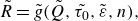 \begin{equation} \tilde {R} = \tilde {g}(\tilde {Q},\tilde {\tau _0},\tilde {\varepsilon },n), \end{equation}
with
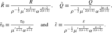 \begin{align} \tilde {R} &\equiv \frac {R}{\rho ^{-\frac {1}{2}} \mu ^{\prime \frac {3}{2(n+1)}} \alpha ^{\frac {n-2}{2(n+1)}}},\quad \tilde {Q} \equiv \frac {Q}{\rho ^{-\frac {3}{2}} \mu ^{\prime \frac {7}{2(n+1)}} \alpha ^{\frac {3n-4}{2(n+1)}}}, \nonumber \\[10pt] \tilde {\tau }_0 &\equiv \frac {\tau _0}{\mu ^{\prime \frac {1}{n+1}} \alpha ^{\frac {n}{n+1}}} \quad\text{ and }\quad \tilde {\varepsilon } \equiv \frac {\varepsilon }{\rho ^{-\frac {1}{2}} \mu ^{\prime \frac {3}{2(n+1)}} \alpha ^{\frac {n-2}{2(n+1)}}} .\end{align}
For convenience, the Reynolds number will be used instead of $\tilde {R}$
. This choice simplifies the calculations and provides direct characterisation of the flow in the channels. Expressed in dimensionless groups, the Reynolds number (2.4) becomes
$\tilde {R}$
. This choice simplifies the calculations and provides direct characterisation of the flow in the channels. Expressed in dimensionless groups, the Reynolds number (2.4) becomes
 \begin{equation} Re= a(n)\frac {\tilde {Q}^{2-n}}{\tilde {R}^{4-3n}}, \end{equation}
where $a(n)$
is defined as
$a(n)$
is defined as
 \begin{equation} a(n) \equiv \frac {8}{\pi ^{2-n}}\left (\frac {n}{3n+1}\right )^n .\end{equation}
In the end, a network can be described by the dimensionless numbers $Re$
,
$Re$
, $\tilde {Q}$
,
$\tilde {Q}$
, $\tilde {\tau }_0$
,
$\tilde {\tau }_0$
, $\tilde {\varepsilon }$
and
$\tilde {\varepsilon }$
and $n$
. All parameters except for
$n$
. All parameters except for $R$
and
$R$
and $Q$
are fluid or system parameters, which are constant in a network. In a branched fluidic network,
$Q$
are fluid or system parameters, which are constant in a network. In a branched fluidic network, $Q$
can change from channel to channel. Therefore, for design procedure purposes, it is convenient that
$Q$
can change from channel to channel. Therefore, for design procedure purposes, it is convenient that $Re$
and
$Re$
and $\tilde {Q}$
are the only flow-rate-dependent dimensionless numbers.
$\tilde {Q}$
are the only flow-rate-dependent dimensionless numbers.
Therefore, the optimisation problem is reduced to the dimensionless dependency
 \begin{equation} Re = \tilde {g}_1(\tilde {Q},\tilde {\tau }_0,\tilde {\varepsilon },n). \end{equation}
For $n=1$
, the dimensionless numbers reduce to
$n=1$
, the dimensionless numbers reduce to
 \begin{equation} Re = \frac {2}{\pi }\frac {\rho Q}{\mu ' R}, \quad \tilde {Q} = \frac {\alpha ^{\frac {1}{4}}\rho ^{\frac {3}{2}} Q}{\mu ^{\prime \frac {7}{4}}},\quad \tilde {\tau }_0 = \frac {\tau _0}{\left (\mu '\alpha \right )^{\frac {1}{2}}} \quad\text{ and }\quad \tilde {\varepsilon } = \frac {\rho ^{\frac {1}{2}}\alpha ^{\frac {1}{4}}\varepsilon }{\mu ^{\prime \frac {3}{4}}} .\end{equation}
For given fluid, flow and system properties, an optimal channel radius can be calculated from the obtained optimal Reynolds number.
A.3 Mapping from 4 to 5 variables for
$f$

The friction factor $f$
commonly depends on the Reynolds number
$f$
commonly depends on the Reynolds number $Re$
, the Hedström number
$Re$
, the Hedström number $He$
, the relative wall roughness
$He$
, the relative wall roughness $\delta$
and the flow index
$\delta$
and the flow index $n$
. These are 4 independent dimensionless groups. In the optimisation procedure, the following 5 dimensionless numbers are used (for details, see Appendix A.2):
$n$
. These are 4 independent dimensionless groups. In the optimisation procedure, the following 5 dimensionless numbers are used (for details, see Appendix A.2): $Re$
,
$Re$
, $\tilde {Q}$
,
$\tilde {Q}$
, $\tilde {\tau }_0$
,
$\tilde {\tau }_0$
, $\tilde {\varepsilon }$
and
$\tilde {\varepsilon }$
and $n$
. Because the friction factor will now be described by 5 instead of 4 dimensionless numbers, a curve in the 5-variable space exists along which
$n$
. Because the friction factor will now be described by 5 instead of 4 dimensionless numbers, a curve in the 5-variable space exists along which $f$
is constant. The direction of that curve is locally described by the vector
$f$
is constant. The direction of that curve is locally described by the vector $\boldsymbol{\beta } = (\beta _1, \beta _2,\beta _3, \beta _4, \beta _5)^T$
. Therefore, the inner product of this vector with the gradient of the original variables
$\boldsymbol{\beta } = (\beta _1, \beta _2,\beta _3, \beta _4, \beta _5)^T$
. Therefore, the inner product of this vector with the gradient of the original variables $\boldsymbol{F} = (Re,He, \delta, n)^T$
to the new variables
$\boldsymbol{F} = (Re,He, \delta, n)^T$
to the new variables $\tilde {\boldsymbol{F}} = (Re,\tilde {Q},\tilde {\tau }_0,\tilde {\varepsilon },n)^T$
must be zero. In that case,
$\tilde {\boldsymbol{F}} = (Re,\tilde {Q},\tilde {\tau }_0,\tilde {\varepsilon },n)^T$
must be zero. In that case, $Re$
,
$Re$
, $He$
,
$He$
, $\delta$
and
$\delta$
and $n$
are constant along the direction of
$n$
are constant along the direction of $\boldsymbol{\beta }$
. This results in the following 4 equations:
$\boldsymbol{\beta }$
. This results in the following 4 equations:
 \begin{equation} \sum _{j=1}^5\frac {\partial {F_i}}{\partial {\tilde {F}_j}}\beta _j =0, \quad \quad \quad i = 1, 2, 3, 4, \end{equation}
which are sufficient to define the direction of the vector $\boldsymbol{\beta }$
while choosing its arbitrary length by conveniently choosing
$\boldsymbol{\beta }$
while choosing its arbitrary length by conveniently choosing $\beta _2 =1$
. Solving (A12) results in
$\beta _2 =1$
. Solving (A12) results in $\beta _1 = 0$
,
$\beta _1 = 0$
, $\beta _3 = -(2n/(4-3n))\ \tilde{\tau}_0 \beta_2 / \tilde{Q}$
,
$\beta _3 = -(2n/(4-3n))\ \tilde{\tau}_0 \beta_2 / \tilde{Q}$
, $\beta _4 = ((2-n)/(4-3n))\ \tilde{\varepsilon} \beta_2 / \tilde{Q}$
and
$\beta _4 = ((2-n)/(4-3n))\ \tilde{\varepsilon} \beta_2 / \tilde{Q}$
and $\beta _5 = 0$
.
$\beta _5 = 0$
.
The function of $f$
will be restricted in the new parameter space by
$f$
will be restricted in the new parameter space by
 \begin{equation} \sum _{j=1}^5\frac {\partial {f}}{\partial {\tilde {F}_j}}\beta _j =0. \end{equation}
Substituting the obtained coefficients $\boldsymbol{\beta }$
results in the following expression:
$\boldsymbol{\beta }$
results in the following expression:
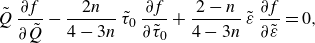 \begin{equation} \tilde {Q}\,\frac {\partial {f}}{\partial {\tilde {Q}}}-\frac {2n}{4-3n}\,\tilde {\tau }_0\,\frac {\partial {f}}{\partial {\tilde {\tau }_0}} + \frac {2-n}{4-3n}\,\tilde {\varepsilon }\,\frac {\partial {f}}{\partial {\tilde {\varepsilon }}} = 0, \end{equation}
which provides the curve along which $f$
is constant in the new parameter space.
$f$
is constant in the new parameter space.
Appendix B. Specific cases of turbulent flow of Newtonian fluid, rough and smooth channel
B.1 Complete turbulence, rough channel
For sufficiently large Reynolds numbers, the friction factor corresponding to fully developed turbulent flow in a circular channel can quite accurately be described by Von Kármán’s formula (Haaland Reference Haaland1983), which holds for rough channels in the limit of high Reynolds numbers
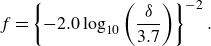 \begin{equation} f = \left \{-2.0\log _{10}\left (\frac {\delta }{3.7}\right )\right \}^{-2}. \end{equation}
This equation is a limit case of the Colebrook–White equation, valid for the complete turbulent regime ( $Re\gt 3500/\delta$
) (Moody Reference Moody1944). In terms of
$Re\gt 3500/\delta$
) (Moody Reference Moody1944). In terms of $\tilde {\varepsilon }$
,
$\tilde {\varepsilon }$
, $\tilde {Q}$
and
$\tilde {Q}$
and $Re$
,
$Re$
, $f$
becomes
$f$
becomes
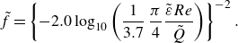 \begin{equation} \tilde {f} = \left \{-2.0\log _{10}\left (\frac {1}{3.7}\,\frac {\pi }{4}\frac {\tilde {\varepsilon }Re}{\tilde {Q}}\right )\right \}^{-2}. \end{equation}
Differentiation to $Re$
results in
$Re$
results in
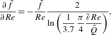 \begin{equation} \frac {\partial {\tilde {f}}}{\partial {Re}} = -\frac {\tilde {f}}{Re}\frac {2}{\ln \left (\dfrac {1}{3.7}\,\dfrac {\pi }{4}\dfrac {\tilde {\varepsilon }Re}{\tilde {Q}}\right ) }, \end{equation}
resulting in
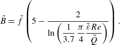 \begin{equation} \tilde {B} = \tilde {f}\left (5- \frac {2}{\ln \left (\dfrac {1}{3.7}\,\dfrac {\pi }{4}\dfrac {\tilde {\varepsilon }Re}{\tilde {Q}}\right ) } \right ). \end{equation}
Contour plots of the optimal $Re$
as function
$Re$
as function $\tilde {Q}$
and
$\tilde {Q}$
and $\tilde {\varepsilon }$
are presented in figure 3(a), for the high-
$\tilde {\varepsilon }$
are presented in figure 3(a), for the high- $\tilde {\varepsilon }$
limit.
$\tilde {\varepsilon }$
limit.
B.2 Turbulence, smooth channel
For a smooth-wall channel ( $\varepsilon \rightarrow 0$
), the Colebrook–White equation (Colebrook Reference Colebrook1939) reduces to
$\varepsilon \rightarrow 0$
), the Colebrook–White equation (Colebrook Reference Colebrook1939) reduces to
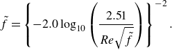 \begin{equation} \tilde {f} = \left \{-2.0\log _{10}\left (\frac {2.51}{Re\sqrt {\tilde {f}}}\right )\right \}^{-2}. \end{equation}
Differentiation to $Re$
gives
$Re$
gives
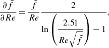 \begin{equation} \frac {\partial {\tilde {f}}}{\partial {Re}} = \frac {\tilde {f}}{Re}\frac {2}{\ln \left (\dfrac {2.51}{Re\sqrt {\tilde {f}}}\right )-1}, \end{equation}
resulting in
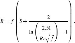 \begin{equation} \tilde {B} = \tilde {f}\left (5+\frac {2}{\ln \left (\dfrac {2.51}{Re\sqrt {\tilde {f}}}\right )-1}\right ). \end{equation}
Figure 5 shows the optimisation curve for $Re$
as function of
$Re$
as function of $\tilde {Q}$
. This result corresponds to the contour plot of the optimal
$\tilde {Q}$
. This result corresponds to the contour plot of the optimal $Re$
as function
$Re$
as function $\tilde {Q}$
and
$\tilde {Q}$
and $\tilde {\varepsilon }$
as presented in figure 3(a) for
$\tilde {\varepsilon }$
as presented in figure 3(a) for $\tilde {\varepsilon }\rightarrow 0$
.
$\tilde {\varepsilon }\rightarrow 0$
.
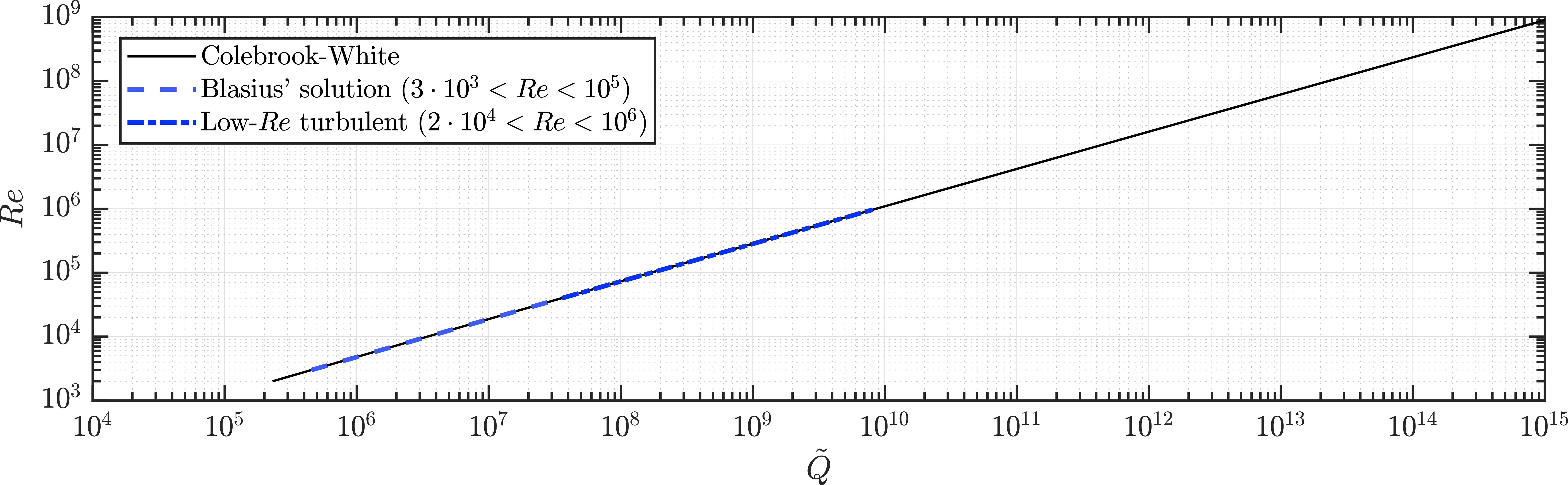
Figure 5. Optimal $Re$
as function of
$Re$
as function of $\tilde {Q}$
for a Newtonian fluid in a smooth-wall channel according to the Colebrook–White equation, together with the Blasius’ formula and a low-
$\tilde {Q}$
for a Newtonian fluid in a smooth-wall channel according to the Colebrook–White equation, together with the Blasius’ formula and a low- $Re$
turbulent approximation.
$Re$
turbulent approximation.
B.3 Low-Reynolds-number turbulence, smooth channel
Power-law approximations for the friction factor have been established for turbulent flows in smooth channels ( $\varepsilon \rightarrow 0$
), for specific and limited ranges of the Reynolds number, in the general form
$\varepsilon \rightarrow 0$
), for specific and limited ranges of the Reynolds number, in the general form
 \begin{equation} \tilde {f} = \frac {c_1}{Re^{c_2}}, \end{equation}
with $c_1$
and
$c_1$
and $c_2$
being two relation-dependent constants. This is an explicit expression for
$c_2$
being two relation-dependent constants. This is an explicit expression for $\tilde {f}$
as function of
$\tilde {f}$
as function of $Re$
, resulting in
$Re$
, resulting in $\tilde {B}$
being
$\tilde {B}$
being
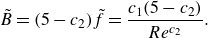 \begin{equation} \tilde {B} = (5-c_2)\tilde {f} = \frac {c_1(5-c_2)}{Re^{c_2}} .\end{equation}
For Newtonian fluids, the optimisation condition (2.12) reduces to
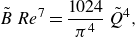 \begin{equation} \tilde {B} \, Re^7=\frac {1024}{\pi ^4}\, \tilde {Q}^4, \end{equation}
which can for this case be rewritten to
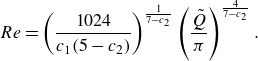 \begin{equation} Re =\left (\frac {1024}{c_1(5-c_2)}\right )^{\frac {1}{7-c_2}}\left (\frac {\tilde {Q}}{\pi }\right )^{\frac {4}{7-c_2}}. \end{equation}
Blasius’ formula (Blasius Reference Blasius1912, Reference Blasius1913), which is valid for $3\times 10^3\lt Re\lt 10^5$
, is given by
$3\times 10^3\lt Re\lt 10^5$
, is given by
 \begin{equation} \tilde {f}=\frac {0.3164}{Re^{\frac {1}{4}}}, \end{equation}
resulting in the optimisation condition
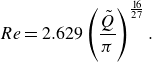 \begin{equation} Re = 2.629\left (\frac {\tilde {Q}}{\pi }\right )^{\frac {16}{27}}. \end{equation}
An empirical relation valid for turbulent flows at intermediate Reynolds numbers ( $2\times 10^4 \lt Re \lt 10^6$
) (Bejan Reference Bejan2013) is given by
$2\times 10^4 \lt Re \lt 10^6$
) (Bejan Reference Bejan2013) is given by
 \begin{equation} \tilde {f}=\frac {0.184}{Re^{\frac {1}{5}}}, \end{equation}
resulting in the optimisation condition
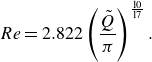 \begin{equation} Re = 2.822\left (\frac {\tilde {Q}}{\pi }\right )^{\frac {10}{17}}. \end{equation}
These explicit expressions for the optimal $Re$
as function of
$Re$
as function of $\tilde {Q}$
are shown in figure 5 for Blasius’ formula (B12) and low-
$\tilde {Q}$
are shown in figure 5 for Blasius’ formula (B12) and low- $Re$
turbulence (B14), revealing perfect coincidence with the more general Colebrook–White solution for smooth channels.
$Re$
turbulence (B14), revealing perfect coincidence with the more general Colebrook–White solution for smooth channels.
Appendix C. Laminar and low-Reynolds-number turbulent flow of Bingham fluid, smooth channel
Considering a turbulent flow of a Bingham fluid in a circular pipe brings to empirical and numerical approximations for the friction factor $f$
. Darby et al. (Darby, Mun & Boger Reference Darby, Mun and Boger1992) developed an empirical curve-fit equation, composed of the following structure:
$f$
. Darby et al. (Darby, Mun & Boger Reference Darby, Mun and Boger1992) developed an empirical curve-fit equation, composed of the following structure:
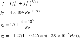 \begin{align} f &= \left (f_L^{\chi _1}+f_T^{\chi _1}\right )^{1/{\chi _1}} \nonumber\\[6pt] f_T &= 4\times 10^{\chi _2}Re^{-0.193} \nonumber\\[6pt] \chi _1 &= 1.7+\frac {4\times 10^5}{Re}\nonumber\\[6pt] \chi _2 &= -1.47(1+0.146\exp (-2.9\times 10^{-5}He)), \end{align}
where $f_L$
is the laminar friction factor as determined from the Buckingham–Reiner (Reiner Reference Reiner1926) equation ((2.18), (3.1) and (3.3) combined).
$f_L$
is the laminar friction factor as determined from the Buckingham–Reiner (Reiner Reference Reiner1926) equation ((2.18), (3.1) and (3.3) combined).
In the new set of dimensionless numbers, the friction factor $\tilde {f}$
becomes
$\tilde {f}$
becomes
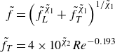 \begin{align*}\tilde {f} &= \left (\tilde {f}_L^{\tilde {\chi }_1}+\tilde {f}_T^{\tilde {\chi }_1}\right )^{1/\tilde {\chi }_1} \nonumber\\[6pt]\tilde {f}_T &= 4\times 10^{\tilde {\chi }_2}Re^{-0.193} \end{align*}
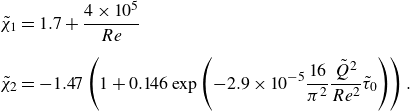 \begin{align}\tilde {\chi }_1 &= 1.7+\frac {4\times 10^5}{Re}\nonumber \\[6pt]\tilde {\chi }_2 &= -1.47\left (1+0.146\exp \left(-2.9\times 10^{-5}\frac {16}{\pi ^2}\frac {\tilde {Q}^2}{Re^2}\tilde {\tau }_0\right)\right).\end{align}
Implicit differentiation of $\tilde {f}$
to
$\tilde {f}$
to $Re$
results in the following expression:
$Re$
results in the following expression:
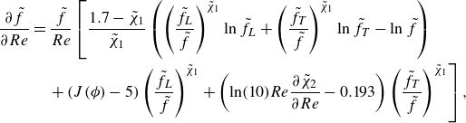 \begin{align} \frac {\partial \tilde {f}}{\partial Re} & = \frac {\tilde {f}}{Re} \left[\frac{1.7-\tilde {\chi }_1}{\tilde {\chi }_1 }\left ( \left (\frac {\tilde {f}_L}{\tilde {f}}\right )^{\tilde {\chi }_1} \ln \tilde {f}_L +\left (\frac {\tilde {f}_T}{\tilde {f}}\right )^{\tilde {\chi }_1} \ln \tilde {f}_T -\ln \tilde {f} \right ) \right.\nonumber \\& \quad \left. +\, (J(\phi )-5)\left (\frac {\tilde {f}_L}{\tilde {f}}\right )^{\tilde {\chi }_1} +\left (\ln (10)Re\frac {\partial \tilde {\chi }_2}{\partial Re}-0.193\right )\left (\frac {\tilde {f}_T}{\tilde {f}}\right )^{\tilde {\chi }_1} \right], \end{align}
where
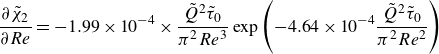 \begin{equation} \frac {\partial \tilde {\chi }_2}{\partial Re} = -1.99\times 10^{-4}\times \frac {\tilde {Q}^2\tilde {\tau }_0}{\pi ^2 Re^3}\exp \left (-4.64\times 10^{-4}\frac {\tilde {Q}^2\tilde {\tau }_0}{\pi ^2 Re^2}\right ) \end{equation}
resulting in
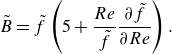 \begin{equation} \tilde {B} = \tilde {f}\left (5+\frac {Re}{\tilde {f}}\frac {\partial {\tilde {f}}}{\partial {Re}}\right ). \end{equation}
The set of equations for this fluid model is relatively complex, but has as benefit that it covers both the laminar and turbulent regimes. The contour plot in figure 6 gives the optimal Reynolds number in a channel for given $\tilde {\tau }_0$
and
$\tilde {\tau }_0$
and $\tilde {Q}$
.
$\tilde {Q}$
.
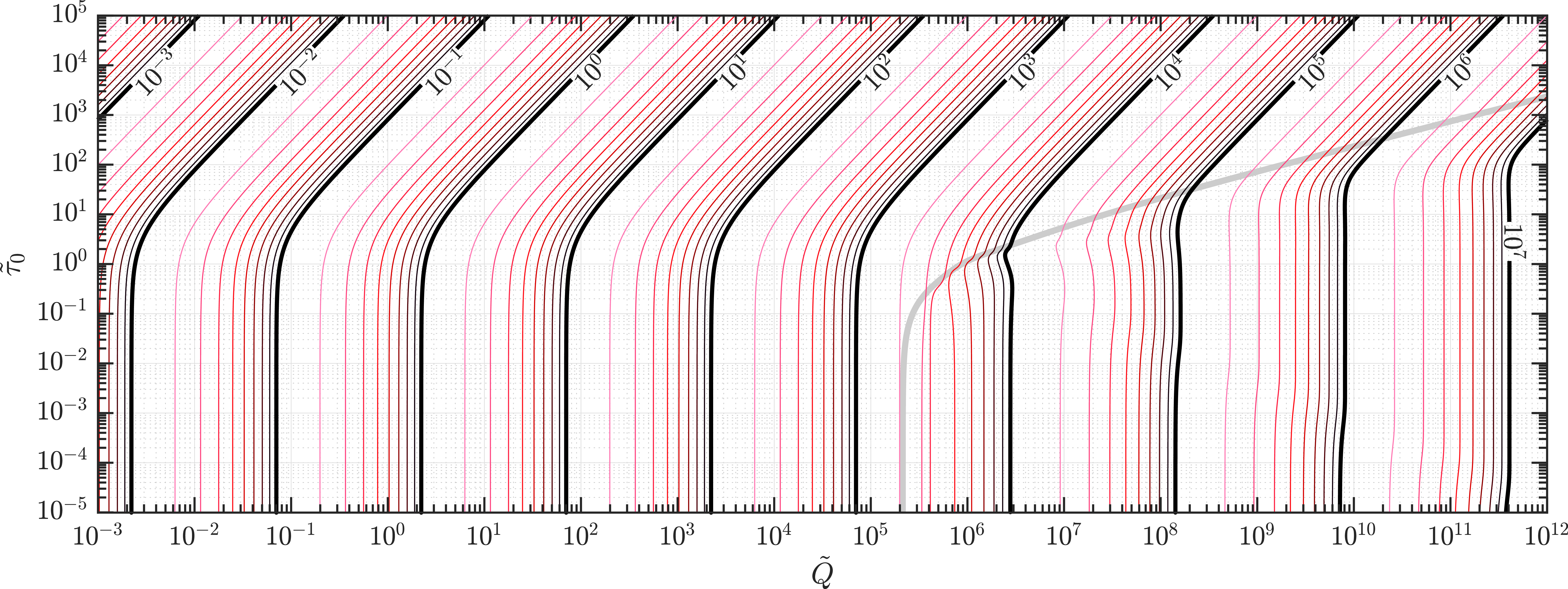
Figure 6. Contour plot of the optimal Reynolds number as a function of $\tilde {Q}$
and
$\tilde {Q}$
and $\tilde {\tau }_0$
, for both laminar and low-Reynolds-number turbulent flow of a Bingham fluid (C1). The red-scale contour lines represent the Reynolds numbers
$\tilde {\tau }_0$
, for both laminar and low-Reynolds-number turbulent flow of a Bingham fluid (C1). The red-scale contour lines represent the Reynolds numbers $2\times 10^x$
,
$2\times 10^x$
, $3\times 10^x$
, …
$3\times 10^x$
, … $9\times 10^x$
with decreasing brightness. The thick grey line represents the critical Reynolds number.
$9\times 10^x$
with decreasing brightness. The thick grey line represents the critical Reynolds number.
Appendix D. Approximation of
$x$
for different fluid models

In network optimisation, many attempts have been made to find the proportionality between the flow rate $Q$
and the channel radius
$Q$
and the channel radius $R$
for optimised networks, in the following form:
$R$
for optimised networks, in the following form:
 \begin{equation} Q\propto R^x .\end{equation}
In the optimisation method of the present study, only $Re$
and
$Re$
and $\tilde {Q}$
contain parameters involving
$\tilde {Q}$
contain parameters involving $R$
and
$R$
and $Q$
, whereas
$Q$
, whereas $\tilde {\tau }_0$
,
$\tilde {\tau }_0$
, $\tilde {\varepsilon }$
and
$\tilde {\varepsilon }$
and $n$
are independent of
$n$
are independent of $R$
and
$R$
and $Q$
. Therefore, when knowing the proportionality between
$Q$
. Therefore, when knowing the proportionality between $\tilde {Q}$
and
$\tilde {Q}$
and $Re$
, one can obtain
$Re$
, one can obtain $x$
using (D1). However, this is only possible if
$x$
using (D1). However, this is only possible if $\tilde {B}\propto Re^{c_1}\tilde {Q}^{c_2}$
. However, in most of the cases (except for e.g. Blasius’ formula), this is not true. Therefore,
$\tilde {B}\propto Re^{c_1}\tilde {Q}^{c_2}$
. However, in most of the cases (except for e.g. Blasius’ formula), this is not true. Therefore, $x$
is calculated by locally approximating
$x$
is calculated by locally approximating $\tilde {B}$
by a power function using
$\tilde {B}$
by a power function using
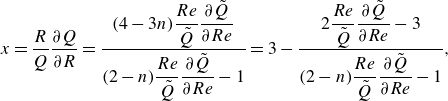 \begin{equation} x = \frac {R}{Q}\frac {\partial Q}{\partial R}= \frac {(4-3n)\dfrac {Re}{\tilde {Q}}\dfrac {\partial {\tilde {Q}}}{\partial {Re}}}{(2-n)\dfrac {Re}{\tilde {Q}}\dfrac {\partial {\tilde {Q}}}{\partial {Re}}-1} = 3-\frac {2\dfrac {Re}{\tilde {Q}}\dfrac {\partial {\tilde {Q}}}{\partial {Re}}-3}{(2-n)\dfrac {Re}{\tilde {Q}}\dfrac {\partial {\tilde {Q}}}{\partial {Re}}-1}, \end{equation}
where $(Re / \tilde{Q}) {\partial {\tilde {Q}}}/{\partial {Re}}$
is derived to be
$(Re / \tilde{Q}) {\partial {\tilde {Q}}}/{\partial {Re}}$
is derived to be
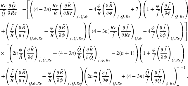 \begin{align} & \frac {Re}{\tilde {Q}}\frac {\partial {\tilde {Q}}}{\partial {Re}} = \!- \!\left [\!\left ((4-3n)\frac {Re}{\tilde {B}}\!\left (\frac {\partial {\tilde {B}}}{\partial {Re}} \right )_{\tilde {f},\tilde {Q},\phi } -4\frac {\phi }{\tilde {B}}\!\left (\frac {\partial {\tilde {B}}}{\partial {\phi }} \right )_{\tilde {f},\tilde {Q},Re} \!+7 \right )\!\left (1+\frac {\phi }{\tilde {f}}\!\left (\frac {\partial {\tilde {f}}}{\partial {\phi }} \right )_{\tilde {Q},Re} \right ) \right. \nonumber \\[3pt]& \left. + \!\left (\frac {\tilde {f}}{\tilde {B}}\!\left (\frac {\partial {\tilde {B}}}{\partial {\tilde {f}}} \right )_{\tilde {Q},\phi, Re}-\frac {\phi }{\tilde {B}}\!\left (\frac {\partial {\tilde {B}}}{\partial {\phi }} \right )_{\tilde {f},\tilde {Q},Re} \right )\!\left ( (4-3n)\frac {Re}{\tilde {f}}\!\left (\frac {\partial {\tilde {f}}}{\partial {Re}} \right )_{\tilde {Q},\phi }-4\frac {\phi }{\tilde {f}}\!\left (\frac {\partial {\tilde {f}}}{\partial {\phi }} \right )_{\tilde {Q},Re} \right )\right ] \nonumber \\[3pt]& \times \left[\!\left (2n\frac {\phi }{\tilde {B}}\!\left (\frac {\partial {\tilde {B}}}{\partial {\phi }} \right )_{\tilde {f},\tilde {Q},Re}+(4-3n)\frac {\tilde {Q}}{\tilde {B}}\!\left (\frac {\partial {\tilde {B}}}{\partial {\tilde {Q}}} \right )_{\tilde {f},\phi, Re}-2(n+1) \right )\!\left (1+\frac {\phi }{\tilde {f}}\!\left (\frac {\partial {\tilde {f}}}{\partial {\phi }} \right )_{\tilde {Q},Re} \right ) \right. \nonumber \\[3pt]& \left. + \!\left (\frac {\tilde {f}}{\tilde {B}}\!\left (\frac {\partial {\tilde {B}}}{\partial {\tilde {f}}} \!\right )_{\tilde {Q},\phi, Re}\!-\frac {\phi }{\tilde {B}}\!\left (\frac {\partial {\tilde {B}}}{\partial {\phi }} \right )_{\tilde {f},\tilde {Q},Re} \!\right )\!\!\left ( 2n\frac {\phi }{\tilde {f}}\!\left (\frac {\partial {\tilde {f}}}{\partial {\phi }} \right )_{\tilde {Q},Re}\!\!+(4-3n)\frac {\tilde {Q}}{\tilde {f}}\!\left (\frac {\partial {\tilde {f}}}{\partial {\tilde {Q}}} \right )_{\phi, Re} \! \right )\! \right ]^{-1}.\end{align}
Equation (D3) is an expression containing 7 differentials of $\tilde {B}$
or
$\tilde {B}$
or $\tilde {f}$
to
$\tilde {f}$
to $Re$
,
$Re$
, $\phi$
,
$\phi$
, $\tilde {f}$
or
$\tilde {f}$
or $\tilde {Q}$
. All differentials can be calculated with keeping the parameters in subscript fixed. The differentials have to be calculated for every flow model separately. The calculated value for
$\tilde {Q}$
. All differentials can be calculated with keeping the parameters in subscript fixed. The differentials have to be calculated for every flow model separately. The calculated value for $x$
is only valid around its corresponding point in the (
$x$
is only valid around its corresponding point in the ( $Re,\tilde {\tau }_0,\tilde {\varepsilon },n$
)-space with a limited range depending on the change in
$Re,\tilde {\tau }_0,\tilde {\varepsilon },n$
)-space with a limited range depending on the change in $x$
. Expressions for the differentials for the fluid models presented in the following sections.
$x$
. Expressions for the differentials for the fluid models presented in the following sections.
D.1 Laminar flow of a Newtonian, power-law, Bingham and Herschel–Bulkley fluids
For a laminar flow, the friction factor was found to be
 \begin{equation} \tilde {f} =\frac {64}{Re \,\psi (\phi, n)^n}, \end{equation}
resulting in an expression for $\tilde {B}$
being
$\tilde {B}$
being
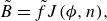 \begin{equation} \tilde {B} = \tilde {f}J(\phi, n), \end{equation}
where $J(\phi, n)$
is defined as
$J(\phi, n)$
is defined as
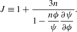 \begin{equation} J\equiv 1+\frac {3n}{1-\dfrac {n\phi }{\psi }\dfrac {\partial {\psi }}{\partial {\phi }}}. \end{equation}
Differentiation provides the needed differentials in (D3), resulting in the expression for $x$
(D2)
$x$
(D2)
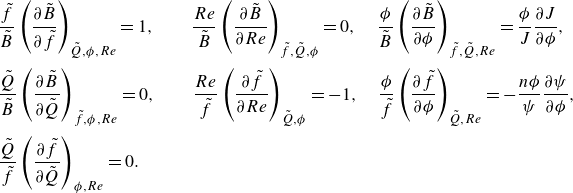 \begin{eqnarray} && \frac {\tilde {f}}{\tilde {B}}\left (\frac {\partial {\tilde {B}}}{\partial {\tilde {f}}}\right )_{\tilde {Q},\phi, Re}=1,\quad \quad \frac {Re}{\tilde {B}}\left (\frac {\partial {\tilde {B}}}{\partial {Re}}\right )_{\tilde {f},\tilde {Q},\phi }=0, \quad \frac {\phi }{\tilde {B}}\left (\frac {\partial {\tilde {B}}}{\partial {\phi }}\right )_{\tilde {f},\tilde {Q},Re}=\frac {\phi }{J}\frac {\partial {J}}{\partial {\phi }}, \nonumber\\[3pt] &&\frac {\tilde {Q}}{\tilde {B}}\left (\frac {\partial {\tilde {B}}}{\partial {\tilde {Q}}}\right )_{\tilde {f},\phi, Re}=0,\quad \quad \frac {Re}{\tilde {f}}\left (\frac {\partial {\tilde {f}}}{\partial {Re}}\right )_{\tilde {Q},\phi } =-1, \quad \frac {\phi }{\tilde {f}}\left (\frac {\partial {\tilde {f}}}{\partial {\phi }}\right )_{\tilde {Q},Re}=-\frac {n\phi }{\psi }\frac {\partial {\psi }}{\partial {\phi }},\nonumber\\[3pt] && \frac {\tilde {Q}}{\tilde {f}}\left (\frac {\partial {\tilde {f}}}{\partial {\tilde {Q}}}\right )_{\phi, Re}=0. \end{eqnarray}
Substituting everything into (D3) results in $(Re / \tilde{Q})\ {\partial {\tilde {Q}}}/{\partial {Re}} = {3}/{2}$
, resulting in
$(Re / \tilde{Q})\ {\partial {\tilde {Q}}}/{\partial {Re}} = {3}/{2}$
, resulting in $x=3$
. This holds for laminar flow of all treated fluid models.
$x=3$
. This holds for laminar flow of all treated fluid models.
D.2 Turbulent flow of Newtonian fluid, rough and smooth channel
A turbulent flow of a Newtonian fluid in a rough or smooth channel can be described by the Colebrook–White equation (Colebrook Reference Colebrook1939), which is in the applied non-dimensionalisation
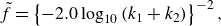 \begin{equation} \tilde {f} = \left \{-2.0\log _{10}\left (k_1+k_2\right )\right \}^{-2}, \end{equation}
with
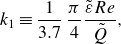 \begin{equation} k_1 \equiv \frac {1}{3.7}\,\frac {\pi }{4}\frac {\tilde {\varepsilon }Re}{\tilde {Q}}, \end{equation}
 \begin{equation} k_2 \equiv \frac {2.51}{\sqrt {\tilde {f}}Re}. \end{equation}
Differentiation provides the needed differentials in (D3)
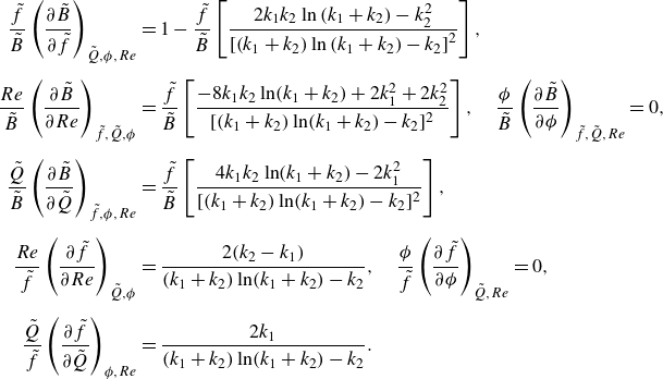 \begin{align} \frac {\tilde {f}}{\tilde {B}}\left (\frac {\partial {\tilde {B}}}{\partial {\tilde {f}}}\right )_{\tilde {Q},\phi, Re} & =1-\frac {\tilde {f}}{\tilde {B}}\left [ \frac {2k_1 k_2\ln \left (k_1+k_2 \right )-k_2^2}{\left [\left (k_1+k_2\right )\ln \left (k_1+k_2\right )-k_2\right ]^{2}}\right ],\nonumber\\[6pt] \frac {Re}{\tilde {B}}\left (\frac {\partial {\tilde {B}}}{\partial {Re}}\right )_{\tilde {f},\tilde {Q},\phi } & =\frac {\tilde {f}}{\tilde {B}}\left [ \frac {-8k_1k_2\ln (k_1+k_2)+2k_1^2+2k_2^2}{[(k_1+k_2)\ln (k_1+k_2)-k_2]^2} \right ],\quad \frac {\phi }{\tilde {B}}\left (\frac {\partial {\tilde {B}}}{\partial {\phi }}\right )_{\tilde {f},\tilde {Q},Re}=0,\nonumber\\[6pt] \frac {\tilde {Q}}{\tilde {B}}\left (\frac {\partial {\tilde {B}}}{\partial {\tilde {Q}}}\right )_{\tilde {f},\phi, Re} & =\frac { \tilde {f}}{\tilde {B}}\left [ \frac {4k_1k_2\ln (k_1+k_2)-2k_1^2}{[(k_1+k_2)\ln (k_1+k_2)-k_2]^2} \right ],\nonumber\\[6pt] \frac {Re}{\tilde {f}}\left (\frac {\partial {\tilde {f}}}{\partial {Re}}\right )_{\tilde {Q},\phi } & =\frac {2(k_2-k_1)}{(k_1+k_2)\ln (k_1+k_2)-k_2},\quad \frac {\phi }{\tilde {f}}\left (\frac {\partial {\tilde {f}}}{\partial {\phi }}\right )_{\tilde {Q},Re}=0,\nonumber\\[6pt] \frac {\tilde {Q}}{\tilde {f}}\left (\frac {\partial {\tilde {f}}}{\partial {\tilde {Q}}}\right )_{\phi, Re} & =\frac {2k_1}{(k_1+k_2)\ln (k_1+k_2)-k_2}. \end{align}
D.2.1 Complete turbulent flow of Newtonian fluid, rough channel
For sufficiently large Reynolds numbers, the friction factor corresponding to complete turbulence in a circular channel can accurately be described by Von Kármán’s formula (Haaland Reference Haaland1983)
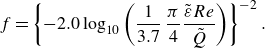 \begin{equation} f = \left \{-2.0\log _{10}\left (\frac {1}{3.7}\,\frac {\pi }{4}\frac {\tilde {\varepsilon }Re}{\tilde {Q}}\right )\right \}^{-2}. \end{equation}
Differentiation provides the needed differentials in (D3)
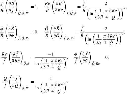 \begin{align} \frac {\tilde {f}}{\tilde {B}}\left (\frac {\partial {\tilde {B}}}{\partial {\tilde {f}}}\right )_{\tilde {Q},\phi, Re} & =1,\quad \frac {Re}{\tilde {B}}\left (\frac {\partial {\tilde {B}}}{\partial {Re}}\right )_{\tilde {f},\tilde {Q},\phi }=\frac {\tilde {f}}{\tilde {B}}\frac {2}{\left (\ln \left (\dfrac {1}{3.7}\,\dfrac {\pi }{4}\dfrac {\tilde {\varepsilon }Re}{\tilde {Q}}\right )\right )^2},\nonumber\\[10pt] \frac {\phi }{\tilde {B}}\left (\frac {\partial {\tilde {B}}}{\partial {\phi }}\right )_{\tilde {f},\tilde {Q},Re} & =0,\quad \frac {\tilde {Q}}{\tilde {B}}\left (\frac {\partial {\tilde {B}}}{\partial {\tilde {Q}}}\right )_{\tilde {f},\phi, Re}=\frac {\tilde {f}}{\tilde {B}}\frac {-2}{\left (\ln \left (\dfrac {1}{3.7}\,\dfrac {\pi }{4}\dfrac {\tilde {\varepsilon }Re}{\tilde {Q}}\right )\right )^2},\nonumber\\[10pt] \frac {Re}{\tilde {f}}\left (\frac {\partial {\tilde {f}}}{\partial {Re}}\right )_{\tilde {Q},\phi } & =\frac {-1}{\ln \left (\dfrac {1}{3.7}\,\dfrac {\pi }{4}\dfrac {\tilde {\varepsilon }Re}{\tilde {Q}}\right )},\quad \frac {\phi }{\tilde {f}}\left (\frac {\partial {\tilde {f}}}{\partial {\phi }}\right )_{\tilde {Q},Re}=0,\nonumber\\[10pt] \frac {\tilde {Q}}{\tilde {f}}\left (\frac {\partial {\tilde {f}}}{\partial {\tilde {Q}}}\right )_{\phi, Re} & =\frac {1}{\ln \left (\dfrac {1}{3.7}\,\dfrac {\pi }{4}\dfrac {\tilde {\varepsilon }Re}{\tilde {Q}}\right )}. \end{align}
D.2.2 Turbulence, smooth channel
For a smooth-wall channel ( $\varepsilon \rightarrow 0$
), the Colebrook–White equation (Colebrook Reference Colebrook1939) reduces to
$\varepsilon \rightarrow 0$
), the Colebrook–White equation (Colebrook Reference Colebrook1939) reduces to
 \begin{equation} \tilde {f} = \left \{-2.0\log _{10}\left (\frac {2.51}{Re\sqrt {\tilde {f}}}\right )\right \}^{-2}. \end{equation}
Differentiation provides the needed differentials in (D3)
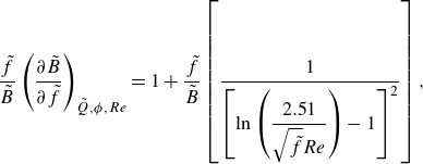 \begin{align*} \ \frac {\tilde {f}}{\tilde {B}}\left (\frac {\partial {\tilde {B}}}{\partial {\tilde {f}}}\right )_{\tilde {Q},\phi, Re}=1+\frac {\tilde {f}}{\tilde {B}}\left [ \frac {1}{\left [\ln \left (\dfrac {2.51}{\sqrt {\tilde {f}}Re}\right )-1\right ]^{2}}\right ], \qquad\qquad\qquad\qquad\qquad\qquad\qquad \end{align*}
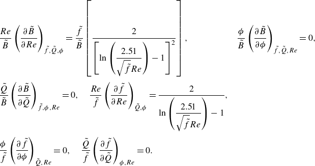 \begin{equation} \begin{aligned} &\frac {Re}{\tilde {B}}\left (\frac {\partial {\tilde {B}}}{\partial {Re}}\right )_{\tilde {f},\tilde {Q},\phi }=\frac {\tilde {f}}{\tilde {B}}\left [ \frac {2}{\left[\ln \left(\dfrac {2.51}{\sqrt {\tilde {f}}Re} \right)-1 \right]^2} \right ],\quad &&\frac {\phi }{\tilde {B}}\left (\dfrac {\partial {\tilde {B}}}{\partial {\phi }}\right )_{\tilde {f},\tilde {Q},Re}=0,\\[3pt] &\frac {\tilde {Q}}{\tilde {B}}\left (\frac {\partial {\tilde {B}}}{\partial {\tilde {Q}}}\right )_{\tilde {f},\phi, Re}=0,\quad \frac {Re}{\tilde {f}}\left (\frac {\partial {\tilde {f}}}{\partial {Re}}\right )_{\tilde {Q},\phi }=\frac {2}{\ln \left(\dfrac {2.51}{\sqrt {\tilde {f}}Re} \right)-1},\\[3pt] &\frac {\phi }{\tilde {f}}\left (\frac {\partial {\tilde {f}}}{\partial {\phi }}\right )_{\tilde {Q},Re}=0,\quad \frac {\tilde {Q}}{\tilde {f}}\left (\frac {\partial {\tilde {f}}}{\partial {\tilde {Q}}}\right )_{\phi, Re}=0. \end{aligned} \end{equation}
D.2.3 Low-Reynolds-number turbulence, smooth channel
For certain Reynolds-number regimes of flow in a smooth channel ( $\varepsilon \rightarrow 0$
), approximations for the friction factor have been formulated, such as Blasius’ formula and empirical relations. These are often in the following form (Uylings Reference Uylings1977):
$\varepsilon \rightarrow 0$
), approximations for the friction factor have been formulated, such as Blasius’ formula and empirical relations. These are often in the following form (Uylings Reference Uylings1977):
 \begin{equation} \tilde {f} = \frac {c_1}{Re^{c_2}} .\end{equation}
Differentiation provides the needed differentials in (D3)
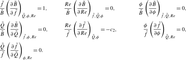 \begin{equation} \begin{aligned} &\frac {\tilde {f}}{\tilde {B}}\left (\frac {\partial {\tilde {B}}}{\partial {\tilde {f}}}\right )_{\tilde {Q},\phi, Re}=1,\quad \quad &&\frac {Re}{\tilde {B}}\left (\frac {\partial {\tilde {B}}}{\partial {Re}}\right )_{\tilde {f},\tilde {Q},\phi }=0,\quad \quad &&&\frac {\phi }{\tilde {B}}\left (\frac {\partial {\tilde {B}}}{\partial {\phi }}\right )_{\tilde {f},\tilde {Q},Re}=0,\\[3pt] &\frac {\tilde {Q}}{\tilde {B}}\left (\frac {\partial {\tilde {B}}}{\partial {\tilde {Q}}}\right )_{\tilde {f},\phi, Re}=0,\quad \quad &&\frac {Re}{\tilde {f}}\left (\frac {\partial {\tilde {f}}}{\partial {Re}}\right )_{\tilde {Q},\phi }=-c_2,\quad \quad &&&\frac {\phi }{\tilde {f}}\left (\frac {\partial {\tilde {f}}}{\partial {\phi }}\right )_{\tilde {Q},Re}=0,\\[3pt] &\frac {\tilde {Q}}{\tilde {f}}\left (\frac {\partial {\tilde {f}}}{\partial {\tilde {Q}}}\right )_{\phi, Re}=0. \end{aligned} \end{equation}
Substituting everything into (D3) results in $(Re / \tilde{Q})\ {\partial {\tilde {Q}}}/{\partial {Re}} =(7-c_2)/4$
, resulting in
$(Re / \tilde{Q})\ {\partial {\tilde {Q}}}/{\partial {Re}} =(7-c_2)/4$
, resulting in $x = (7-c_2)/(3-c_2)$
. For Blasius’ equation (B12),
$x = (7-c_2)/(3-c_2)$
. For Blasius’ equation (B12), $x$
reduces to
$x$
reduces to $x = {27}/{11}$
and for the empirical relation (B14)
$x = {27}/{11}$
and for the empirical relation (B14) $x$
reduces to
$x$
reduces to $x= {17}/{7}$
.
$x= {17}/{7}$
.
D.3 Turbulent flow of non-Newtonian fluids, smooth channel
D.3.1 Power-law fluid
Turbulent pipe flow of non-Newtonian power-law fluids at low Reynolds numbers in a smooth circular channel ( $\varepsilon \rightarrow 0$
) described by Dodge and Metzner (Dodge & Metzner Reference Dodge and Metzner1959) is given in the following implicit relation for the Darcy friction factor
$\varepsilon \rightarrow 0$
) described by Dodge and Metzner (Dodge & Metzner Reference Dodge and Metzner1959) is given in the following implicit relation for the Darcy friction factor $f$
:
$f$
:
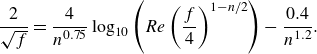 \begin{equation} \frac {2}{\sqrt {f}}=\frac {4}{n^{0.75}}\log _{10}\left (Re\left (\frac {f}{4}\right )^{1-n/2}\right )-\frac {0.4}{n^{1.2}} .\end{equation}
Differentiation provides the needed differentials in (D3)
 \begin{equation} \begin{aligned} &\frac {\tilde {f}}{\tilde {B}}\left (\frac {\partial {\tilde {B}}}{\partial {\tilde {f}}}\right )_{\tilde {Q},\phi, Re}=1-\frac {\tilde {f}}{\tilde {B}}(4-3n)\left (\frac {n^{0.75}\ln (10)}{4\sqrt {\tilde {f}}}+1-\frac {n}{2}\right )^{-2} \frac {n^{0.75}\ln (10)}{8\sqrt {\tilde {f}}},\\[3pt] &\frac {Re}{\tilde {B}}\left (\frac {\partial {\tilde {B}}}{\partial {Re}}\right )_{\tilde {f},\tilde {Q},\phi }=0,\quad \quad \frac {\phi }{\tilde {B}}\left (\frac {\partial {\tilde {B}}}{\partial {\phi }}\right )_{\tilde {f},\tilde {Q},Re}=0,\quad \quad \frac {\tilde {Q}}{\tilde {B}}\left (\frac {\partial {\tilde {B}}}{\partial {\tilde {Q}}}\right )_{\tilde {f},\phi, Re}=0,\\[3pt] &\frac {Re}{\tilde {f}}\left (\frac {\partial {\tilde {f}}}{\partial {Re}}\right )_{\tilde {Q},\phi }=-\left (\frac {n^{0.75}\ln (10)}{4\sqrt {\tilde {f}}}+1-\frac {n}{2}\right )^{-1},\\[3pt] &\frac {\phi }{\tilde {f}}\left (\frac {\partial {\tilde {f}}}{\partial {\phi }}\right )_{\tilde {Q},Re}=0,\quad \quad \quad \frac {\tilde {Q}}{\tilde {f}}\left (\frac {\partial {\tilde {f}}}{\partial {\tilde {Q}}}\right )_{\phi, Re}=0. \end{aligned} \end{equation}
Figure 7. Friction factor as function of the Reynolds number for Herschel–Bulkley fluids. The dashed black line indicates the transition from laminar to turbulent flow. The red-scale lines represent constant values of the Hedström number from $10^{1}, 10^2, \ldots, 10^{10}$
with decreasing brightness.Panels show (a)
$10^{1}, 10^2, \ldots, 10^{10}$
with decreasing brightness.Panels show (a) $n=0.5$
and (b)
$n=0.5$
and (b) $n=1.5$
.
$n=1.5$
.
D.3.2 Herschel–Bulkley fluid
For a turbulent flow of a Herschel–Bulkley fluid in a smooth circular channel ( $\varepsilon \rightarrow 0$
), Torrance (Garcia & Steffe Reference Garcia and Steffe1986) developed a relationship for the Darcy friction factor
$\varepsilon \rightarrow 0$
), Torrance (Garcia & Steffe Reference Garcia and Steffe1986) developed a relationship for the Darcy friction factor
 \begin{equation} \frac {2}{\sqrt {\tilde {f}}}=0.45-\frac {2.75}{n}+\frac {1.97}{n}\ln (1-\phi ) +\frac {1.97}{n}\ln \left (Re\left (\frac {3n+1}{4n}\right )^n \left (\frac {\tilde {f}}{4}\right )^{1-\frac {n}{2}}\right ). \end{equation}
Differentiation provides the needed differentials in (D3)
 \begin{equation} \begin{aligned} &\frac {\tilde {f}}{\tilde {B}}\left (\frac {\partial {\tilde {B}}}{\partial {\tilde {f}}}\right )_{\tilde {Q},\phi, Re}=1-\frac {\tilde {f}}{\tilde {B}}\frac {4-3n+\frac {4\phi }{1-\phi }}{\left ( \frac {n}{1.97\sqrt {\tilde {f}}}+\frac {\phi }{1-\phi }+1-\frac {n}{2} \right )}\frac {\frac {1}{2}n}{1.97\sqrt {\tilde {f}}},\\[3pt] &\frac {Re}{\tilde {B}}\left (\frac {\partial {\tilde {B}}}{\partial {Re}}\right )_{\tilde {f},\tilde {Q},\phi }=0,\quad \quad \frac {\phi }{\tilde {B}}\left (\frac {\partial {\tilde {B}}}{\partial {\phi }}\right )_{\tilde {f},\tilde {Q},Re}=-\frac { \tilde {f}}{\tilde {B}} \frac {\left (\frac {4n}{1.97\sqrt {\tilde {f}}}+n\right )\frac {\phi }{(1-\phi )^2} }{\left (\frac {n}{1.97\sqrt {\tilde {f}}}+\frac {\phi }{1-\phi }+1-\frac {n}{2}\right )^2},\\[3pt] &\frac {\tilde {Q}}{\tilde {B}}\left (\frac {\partial {\tilde {B}}}{\partial {\tilde {Q}}}\right )_{\tilde {f},\phi, Re}=0,\quad \quad \frac {Re}{\tilde {f}}\left (\frac {\partial {\tilde {f}}}{\partial {Re}}\right )_{\tilde {Q},\phi }=\frac {-1}{\frac {n}{1.97\sqrt {\tilde {f}}}+1-\frac {n}{2}},\\[3pt] &\frac {\phi }{\tilde {f}}\left (\frac {\partial {\tilde {f}}}{\partial {\phi }}\right )_{\tilde {Q},Re}=\frac {\frac {\phi }{1-\phi }}{\frac {n}{1.97\sqrt {\tilde {f}}}+1-\frac {n}{2}},\quad \quad \frac {\tilde {Q}}{\tilde {f}}\left (\frac {\partial {\tilde {f}}}{\partial {\tilde {Q}}}\right )_{\phi, Re}=0. \end{aligned} \end{equation}
Appendix E. Extra figures for Herschel–Bulkley fluids (
$\boldsymbol{n}\ \textbf{=}\ \textbf{0.5}$
and
$\boldsymbol{n}\ \textbf{=}\ \textbf{1.5}$
)


For a Herschel–Bulkley fluid, the graphs for the friction factor as function of the Reynolds number and the optimisation graphs have to be made for every value of $n$
separately. For readability, in the main text, it is chosen to limit to
$n$
separately. For readability, in the main text, it is chosen to limit to $n=1$
, and therefore, the graphs for other values of
$n=1$
, and therefore, the graphs for other values of $n$
are given in this section. Figure 7 shows the friction factor
$n$
are given in this section. Figure 7 shows the friction factor $f$
as function of the Reynolds number
$f$
as function of the Reynolds number $Re$
for both laminar and turbulent flow. The optimisation graphs for laminar flow of a Herschel–Bulkley fluid for
$Re$
for both laminar and turbulent flow. The optimisation graphs for laminar flow of a Herschel–Bulkley fluid for $n=0.5$
,
$n=0.5$
, $n=1.0$
and
$n=1.0$
and $n=1.5$
and covering all
$n=1.5$
and covering all $n$
are given in figure 8. The optimisation graphs for turbulent flow for
$n$
are given in figure 8. The optimisation graphs for turbulent flow for $n=0.5$
and
$n=0.5$
and $n=1.5$
are given in figure 9. Finally, figure 10 shows
$n=1.5$
are given in figure 9. Finally, figure 10 shows $x$
as function of
$x$
as function of $Re$
for
$Re$
for $n=0.5$
and
$n=0.5$
and $n=1.5$
.
$n=1.5$
.
Figure 8. Contour plots of the optimisation condition for a laminar flow of a Herschel–Bulkley fluid (3.8). The red-scale contour lines represent values $2\times 10^x$
,
$2\times 10^x$
, $3\times 10^x$
, …
$3\times 10^x$
, … $9\times 10^x$
with decreasing brightness. (a) Optimal Reynolds number as a function of
$9\times 10^x$
with decreasing brightness. (a) Optimal Reynolds number as a function of $\tilde {\tau }_0$
and
$\tilde {\tau }_0$
and $\tilde {Q}$
for a Herschel–Bulkley fluid with
$\tilde {Q}$
for a Herschel–Bulkley fluid with $n=0.5$
. (b) Optimal Reynolds number as a function of
$n=0.5$
. (b) Optimal Reynolds number as a function of $\tilde {\tau }_0$
and
$\tilde {\tau }_0$
and $\tilde {Q}$
for a Herschel–Bulkley fluid with
$\tilde {Q}$
for a Herschel–Bulkley fluid with $n=1.0$
. (c) Optimal Reynolds number as a function of
$n=1.0$
. (c) Optimal Reynolds number as a function of $\tilde {\tau }_0$
and
$\tilde {\tau }_0$
and $\tilde {Q}$
for a Herschel–Bulkley fluid with
$\tilde {Q}$
for a Herschel–Bulkley fluid with $n=1.5$
. (d) Optimal
$n=1.5$
. (d) Optimal $\tilde {R}^3/\tilde {Q}$
as function of
$\tilde {R}^3/\tilde {Q}$
as function of $n$
and
$n$
and $\tilde {\tau }_0$
. This optimisation plot covers all laminar flows of Herschel–Bulkley fluids.
$\tilde {\tau }_0$
. This optimisation plot covers all laminar flows of Herschel–Bulkley fluids.
Figure 9. Contour plots of the optimal Reynolds number as a function of $\tilde {Q}$
and
$\tilde {Q}$
and $\tilde {\tau }_0$
for a turbulent flow of a Herschel–Bulkley fluid (3.17) at constant
$\tilde {\tau }_0$
for a turbulent flow of a Herschel–Bulkley fluid (3.17) at constant $n$
. The red-scale contour lines represent the Reynolds numbers
$n$
. The red-scale contour lines represent the Reynolds numbers $2\times 10^x$
,
$2\times 10^x$
, $3\times 10^x$
, …
$3\times 10^x$
, … $9\times 10^x$
with decreasing brightness. Panels show (a)
$9\times 10^x$
with decreasing brightness. Panels show (a) $n=0.5$
and (b)
$n=0.5$
and (b) $n=1.5$
.
$n=1.5$
.
Figure 10. Plot of $x$
(4.1) as function of
$x$
(4.1) as function of $Re$
for turbulent flow of a Herschel–Bulkley fluid (Torrance) as discussed in § 3.3.2. The dashed lines for
$Re$
for turbulent flow of a Herschel–Bulkley fluid (Torrance) as discussed in § 3.3.2. The dashed lines for $x=3$
and
$x=3$
and $x=7/3$
show the expected limit cases for laminar flow and high-turbulent flow, respectively (Uylings Reference Uylings1977). The different lines are for
$x=7/3$
show the expected limit cases for laminar flow and high-turbulent flow, respectively (Uylings Reference Uylings1977). The different lines are for $\tilde {\tau }_0 \in [0.1,0.25,1,2.5,10,25]$
. Panels show (a)
$\tilde {\tau }_0 \in [0.1,0.25,1,2.5,10,25]$
. Panels show (a) $n= 0.5$
and (b)
$n= 0.5$
and (b) $n= 1.5$
.
$n= 1.5$
.
Figure 11. Example of optimisation of a branched fluidic network for a water distribution network. (a) The position coordinates of the begin point and the endpoints are given and represented by black circles, where the endpoints are located equidistantly along an arc with a radius of curvature of 4 m. (b) The obtained optimised water distribution network. The colour indicates the Reynolds number of the flow within the channel. For visibility, the channel diameters are magnified in the plot.
Appendix F. Example of network optimisation
In this section, an example illustrates how the optimisation theory could be applied. Imagine a water distribution system, which aims to distribute water from a main channel to 8 endpoints. The requested output at each endpoint is 12.5 l min $^{-1}$
, which means that the main channel should supply
$^{-1}$
, which means that the main channel should supply $Q_0$
= 100 l min
$Q_0$
= 100 l min $^{-1}$
. The begin node is at (0,0) and the end nodes are chosen to be placed equidistantly along an arc with a radius of curvature of 4 m (see figure 11
a). It is chosen to have symmetric bifurcations, with 4 levels of branchings, denoted by indices 0 to 3. The channels are drawn tubes with a wall roughness of
$^{-1}$
. The begin node is at (0,0) and the end nodes are chosen to be placed equidistantly along an arc with a radius of curvature of 4 m (see figure 11
a). It is chosen to have symmetric bifurcations, with 4 levels of branchings, denoted by indices 0 to 3. The channels are drawn tubes with a wall roughness of $\varepsilon = 0.0025\,\rm mm$
, and water is a Newtonian fluid (
$\varepsilon = 0.0025\,\rm mm$
, and water is a Newtonian fluid ( $n=1$
,
$n=1$
, $\tau _0=0$
) with viscosity
$\tau _0=0$
) with viscosity $\mu '=1$
mPa s and fluid density
$\mu '=1$
mPa s and fluid density $\rho =1000$
kg m
$\rho =1000$
kg m $^{-3}$
.
$^{-3}$
.
The design procedure as described in § 5 is followed. In step (i), the cost factor could be chosen or derived from a constraint (see also Smink et al. Reference Smink, Venner, Visser and Hagmeijer2023). Here, for the optimisation is chosen to base the cost factor on a constraint for the outlet channel size. The radius of the outlet channels is chosen to be $R_3=7.5\,\rm mm$
, a common channel size for tap water. The cost factor can be retrieved in the following manner. The Reynolds number of the flow in the outlet channels is set by the constraint to be
$R_3=7.5\,\rm mm$
, a common channel size for tap water. The cost factor can be retrieved in the following manner. The Reynolds number of the flow in the outlet channels is set by the constraint to be $Re_3 = 1.768\times 10^4$
. This means that we have a turbulent flow of a Newtonian fluid in rough-wall channels in the network. From the given parameters, it is known that
$Re_3 = 1.768\times 10^4$
. This means that we have a turbulent flow of a Newtonian fluid in rough-wall channels in the network. From the given parameters, it is known that $\tilde {Q}\alpha ^{-1/4} = \rho ^{3/2}\mu ^{\prime -7/4}Q = 1.17\times 10^6$
m
$\tilde {Q}\alpha ^{-1/4} = \rho ^{3/2}\mu ^{\prime -7/4}Q = 1.17\times 10^6$
m $^{3/4}$
W
$^{3/4}$
W $^{-1/4}$
and
$^{-1/4}$
and $\tilde {\varepsilon }\alpha ^{-1/4}=\rho ^{1/2}\mu ^{\prime -3/4}\varepsilon = 0.0141$
m
$\tilde {\varepsilon }\alpha ^{-1/4}=\rho ^{1/2}\mu ^{\prime -3/4}\varepsilon = 0.0141$
m $^{3/4}$
W
$^{3/4}$
W $^{-1/4}$
. We will use the graphical approach to avoid tedious calculations. Figure 3(a) shows the corresponding optimisation graph, using which the combination of
$^{-1/4}$
. We will use the graphical approach to avoid tedious calculations. Figure 3(a) shows the corresponding optimisation graph, using which the combination of $Re$
,
$Re$
, $\tilde {Q}\alpha ^{-1/4}$
and
$\tilde {Q}\alpha ^{-1/4}$
and $\tilde {\varepsilon }\alpha ^{-1/4}$
gives the corresponding
$\tilde {\varepsilon }\alpha ^{-1/4}$
gives the corresponding $\tilde {Q}$
,
$\tilde {Q}$
, $\tilde {\varepsilon }$
and
$\tilde {\varepsilon }$
and $\alpha$
. This graph shows that the given combination shows that
$\alpha$
. This graph shows that the given combination shows that $\tilde {Q}_3\approx 9.0\times 10^6$
,
$\tilde {Q}_3\approx 9.0\times 10^6$
, $\tilde {\varepsilon }\approx 0.11$
and
$\tilde {\varepsilon }\approx 0.11$
and $\alpha \approx 3.5\times 10^3$
W m
$\alpha \approx 3.5\times 10^3$
W m $^{-3}$
. The dimensionless flow rates in the other three levels are then
$^{-3}$
. The dimensionless flow rates in the other three levels are then $\tilde {Q}_2 \approx 1.8\times 10^7$
,
$\tilde {Q}_2 \approx 1.8\times 10^7$
, $\tilde {Q}_1 \approx 3.6\times 10^7$
and
$\tilde {Q}_1 \approx 3.6\times 10^7$
and $\tilde {Q}_0 \approx 7.2\times 10^7$
.
$\tilde {Q}_0 \approx 7.2\times 10^7$
.
In step (ii), the optimal radius for one channel is determined. In this case, the channel radius and Reynolds number for the outlet channels (level 3) are already known because of the given constraint. Step (iii) is then carried out for obtaining the other optimal channel radii $R_i$
via the optimal Reynolds numbers in the channels, by repeating step (ii) for each channel. Using
$R_i$
via the optimal Reynolds numbers in the channels, by repeating step (ii) for each channel. Using $\tilde {\varepsilon }$
and the determined
$\tilde {\varepsilon }$
and the determined $\tilde {Q}_i$
(
$\tilde {Q}_i$
( $i=0,1,2,3$
), the other optimal values of
$i=0,1,2,3$
), the other optimal values of $Re_i$
are obtained from figure 3(a). These are
$Re_i$
are obtained from figure 3(a). These are $Re_2 \approx 2.6\times 10^4$
,
$Re_2 \approx 2.6\times 10^4$
, $Re_1 \approx 4.0\times 10^4$
and
$Re_1 \approx 4.0\times 10^4$
and $Re_0 \approx 6.0\times 10^4$
. From here, the channel radii are calculated using the definition of the Reynolds number (2.4):
$Re_0 \approx 6.0\times 10^4$
. From here, the channel radii are calculated using the definition of the Reynolds number (2.4): $R_2 \approx 10.2\,\rm mm$
,
$R_2 \approx 10.2\,\rm mm$
, $R_1 \approx 13.3\,\rm mm$
,
$R_1 \approx 13.3\,\rm mm$
, $R_0 \approx 17.7\,\rm mm$
. These are the optimised channel radii. Finally, the positions of the branching point locations are calculated in step (iv) (see Appendix A.1), resulting in the full geometry of the optimised water distribution network, presented in figure 11(b). In each level, the lengths of the channels are the same (
$R_0 \approx 17.7\,\rm mm$
. These are the optimised channel radii. Finally, the positions of the branching point locations are calculated in step (iv) (see Appendix A.1), resulting in the full geometry of the optimised water distribution network, presented in figure 11(b). In each level, the lengths of the channels are the same ( $L_0 \approx 5.71\,\rm $
,
$L_0 \approx 5.71\,\rm $
, $L_1 \approx 1.48\,\rm $
,
$L_1 \approx 1.48\,\rm $
, $L_2\approx 1.80\,\rm $
and
$L_2\approx 1.80\,\rm $
and $L_3\approx 1.18\,\rm m$
), and therefore the same holds for the pressure drop in the channels in each level (
$L_3\approx 1.18\,\rm m$
), and therefore the same holds for the pressure drop in the channels in each level ( $\Delta p_0 \approx 4.85\,\rm $
,
$\Delta p_0 \approx 4.85\,\rm $
, $\Delta p_1 \approx 1.42\,\rm $
,
$\Delta p_1 \approx 1.42\,\rm $
, $\Delta p_2\approx 1.97\,\rm $
and
$\Delta p_2\approx 1.97\,\rm $
and $\Delta p_3\approx 1.47\,\rm kPa$
).
$\Delta p_3\approx 1.47\,\rm kPa$
).


 Open access