


1. Introduction
NT Aps (HD 128575) is a poorly studied southern (RA = 14 42 42.5763013776, DEC = −74 18 41.568175368) eclipsing binary system, situated 54.071 pc away from the Sun (Gaia Collaboration 2020). The first reported photometric observations by Strohmeier, Knigge, & Ott (Reference Strohmeier, Knigge and Ott1965) indicated variations in the light curve with an amplitude of $0.3^{m}$
. The Hipparcos input catalogue v.2 (Turon et al. Reference Turon1993) provided an estimated spectral classification of G3/G5 V for both components, confirmed by the New Reduction (Van Leeuwen Reference Van Leeuwen2007), which obtained B-V colour index of 0.630
$0.3^{m}$
. The Hipparcos input catalogue v.2 (Turon et al. Reference Turon1993) provided an estimated spectral classification of G3/G5 V for both components, confirmed by the New Reduction (Van Leeuwen Reference Van Leeuwen2007), which obtained B-V colour index of 0.630 $\pm$
0.013. Later, NT Aps was classified as a W UMa-type eclipsing binary by Kazarovets et al. (Reference Kazarovets, Samus, Durlevich, Frolov, Antipin, Kireeva and Pastukhova1999). The list of eclipsing variables by Avvakumova, Malkov, & Kniazev (Reference Avvakumova, Malkov and Kniazev2013) puts NT Aps in the CWW evolutionary class, which is a late-type contact W UMa system of sub-type W.
$\pm$
0.013. Later, NT Aps was classified as a W UMa-type eclipsing binary by Kazarovets et al. (Reference Kazarovets, Samus, Durlevich, Frolov, Antipin, Kireeva and Pastukhova1999). The list of eclipsing variables by Avvakumova, Malkov, & Kniazev (Reference Avvakumova, Malkov and Kniazev2013) puts NT Aps in the CWW evolutionary class, which is a late-type contact W UMa system of sub-type W.
According to Binnendijk (Reference Binnendijk1970), W UMa binaries can be classified into two sub-types: A-type, for which an occultation occurs during the primary minimum, the primary star has the higher temperature and the stars are generally of earlier spectral types, and W-type, for which there is a transit during the primary minimum, the primary has the lower temperature and the stars are of later spectral types. Other differences include lower mass ratios ( $q \lt 3.7$
, Lucy & Wilson Reference Lucy and Wilson1979) and longer periods (Smith Reference Smith1984) for the A-type. In addition, Lucy & Wilson (Reference Lucy and Wilson1979) proposed the existence of B-type systems based on photometric data from three systems with surface temperature differences between the components
$q \lt 3.7$
, Lucy & Wilson Reference Lucy and Wilson1979) and longer periods (Smith Reference Smith1984) for the A-type. In addition, Lucy & Wilson (Reference Lucy and Wilson1979) proposed the existence of B-type systems based on photometric data from three systems with surface temperature differences between the components $(T_1-T_2$
) more than 270 K. This indicates systems with geometrical contact but poor thermal contact. Acerbi, Barani, & Popov (Reference Acerbi, Barani and Popov2022) suggested H-type sub-class systems with a mass ratio greater than 0.72 and a lower energy transfer rate.
$(T_1-T_2$
) more than 270 K. This indicates systems with geometrical contact but poor thermal contact. Acerbi, Barani, & Popov (Reference Acerbi, Barani and Popov2022) suggested H-type sub-class systems with a mass ratio greater than 0.72 and a lower energy transfer rate.
Pilecki & Stepien (Reference Pilecki and Stepien2012) investigated the light curve models of W UMa-type variables characterised by orbital periods less than 0.3 days and total mass below 1.4 solar masses. For NT Aps they obtained temperature ratio of 0.951, inclination 72.1 deg, and mass ratio 0.25.
The study of W UMa systems (short-period eclipsing binary stars) enhances our understanding of stellar astrophysics by revealing how close binary stars form, evolve, and interact. Analysing the light curves and the characteristics of the brightness variations provides valuable information about the sizes, temperatures, and masses of the stars in the system. By studying the spectral lines, one can deduce the chemical composition, temperature, and surface gravity of the stars, as well as better constrain the masses. Also, cool contact binaries can merge due to the interaction between the evolutionary expansion of the less massive component, which transfers mass to the more massive component (Webbink Reference Webbink1977; Stepien & Gazeas Reference Stepien and Gazeas2012). The orbital period decreases until the binary overflows the outer critical Roche surface and merges into a fast-rotating solar-like star with a residual disc bearing excess angular momentum.
Middleton (Reference Middleton2012) reported the results of photometric observations of NT Aps in white light during 2007, as well as observations done using B and V filters from 2008. He presented light curve modelling using Binary Maker 3 and Phoebe, gave estimates of the parameters of the binary and established an O-C effect indicative of a period decrease. Nevertheless, he noted that the presence of spectral measurements is necessary in order to achieve more accurate modelling.
Here we report on the results from the first combined spectroscopic and photometric study of NT Aps. To our knowledge, there are no previous spectroscopic studies of this system in the literature.
2. Observations, data reduction, and measurements
The study of NT Aps is part of our wider investigation of flares and coronal mass ejections (CMEs) on M dwarfs and solar-like stars (to be published separately). The system was selected based on the results from Leitzinger et al. (Reference Leitzinger2020), who present an estimated flare rate $\approx$
95.12 per day in EUV (calculated using the EUV power law from Audard et al. Reference Audard, Güdel, Drake and Kashyap2000) and flare rate in H
$\approx$
95.12 per day in EUV (calculated using the EUV power law from Audard et al. Reference Audard, Güdel, Drake and Kashyap2000) and flare rate in H $\alpha \approx$
5.19 per day. The magnetic activity and chromospheric features of the components of systems like NT Aps can be affected by tidal effects, mass transfer, and combining of the envelopes, the latter creating more complex magnetic fields and thus enhancing chromospheric activity. For analysis of the latter, among the most commonly used features are the H
$\alpha \approx$
5.19 per day. The magnetic activity and chromospheric features of the components of systems like NT Aps can be affected by tidal effects, mass transfer, and combining of the envelopes, the latter creating more complex magnetic fields and thus enhancing chromospheric activity. For analysis of the latter, among the most commonly used features are the H $\alpha$
and Ca II spectral lines.
$\alpha$
and Ca II spectral lines.
2.1 Spectroscopy
We observed NT Aps using the European Southern Observatory’s Faint Object Spectrograph and Camera v.2 (EFOSC2) attached to the New Technology Telescope (NTT) on La Silla (for more details on the instrument, see Buzzoni et al. Reference Buzzoni1984; Snodgrass et al. Reference Snodgrass, Saviane, Monaco and Sinclaire2008). We used grism Gr#20 together with the 0.5′′ slit (Slit#0.5), resulting in wavelength coverage of 605 – 715 nm and resolving power ( $\lambda/\delta\lambda$
) of some 6 000.
$\lambda/\delta\lambda$
) of some 6 000.
We used 124 spectra collected from the system in two separate nights on April 29, 2021 and June 30, 2023. The observations collected in 2021 were from ESO programme ID 60.A-9709(D), and the ones in 2023 were part of our proposal No 111.254K. Both datasets have similar data quality with an average signal-to-noise-ratio of $\sim$
100 and individual spectra ranging from 56 to 158. Table 1 presents details of the observations: date, number of obtained spectra and exposure time. In 2023, the exposure time varies from 90 to 120 s to account for changing atmospheric conditions. Our main study focuses on stellar coronal mass ejections and does not require high radial velocity precision, therefore we did not observe a radial velocity standard.
$\sim$
100 and individual spectra ranging from 56 to 158. Table 1 presents details of the observations: date, number of obtained spectra and exposure time. In 2023, the exposure time varies from 90 to 120 s to account for changing atmospheric conditions. Our main study focuses on stellar coronal mass ejections and does not require high radial velocity precision, therefore we did not observe a radial velocity standard.
Table 1. Log of the spectroscopic observations of NT Aps.

To execute standard processing of the obtained spectra we used the IRAF software package (Tody Reference Tody1986, Reference Tody1993). A heliocentric correction was applied to all the data. The radial velocities of the two components of the eclipsing binary system were calculated using the package splot with a fit function. In case of lower S/N ratio, we used a boxcar function to smooth out the continuum and better distinguish the lines. Then we used Gaussian functions to fit the lines of the two components separately, and in combination. The latter was done to check how accurate the measured line centres were. Using the standard formula for the Doppler shift, we obtained the radial velocities for each component. They are listed in Table 6 in Appendix A.
The resulting spectra from the observations are shown in Fig. 1a for epoch 2021 and Fig. 1b for epoch 2023, respectively. To further search for activity indications, we also generated dynamic spectra in the H $\alpha$
region for each observation using an IDL-based code. These are shown in Fig. 1c and d, respectively. The white area in the dynamic spectra in Fig. 1c indicates a gap in the observational data. Although no signatures of activity are present, the evolution of the H
$\alpha$
region for each observation using an IDL-based code. These are shown in Fig. 1c and d, respectively. The white area in the dynamic spectra in Fig. 1c indicates a gap in the observational data. Although no signatures of activity are present, the evolution of the H $\alpha$
line profiles due to the motion of the binary components can be seen clearly.
$\alpha$
line profiles due to the motion of the binary components can be seen clearly.

Figure 1. Evolution of the observed H $\alpha$
profile and dynamic spectra from epochs 2021 and 2023. The change of the line profiles due to the orbital motion of the two components is clearly visible.
$\alpha$
profile and dynamic spectra from epochs 2021 and 2023. The change of the line profiles due to the orbital motion of the two components is clearly visible.
2.2 Photometry
For the photometric analysis, we used the complete set of observational data obtained from the Transiting Exoplanet Survey Satellite (TESS, Ricker et al. Reference Ricker2014) up to, and including, sector 66. At the time of the analysis, data related to the NT Aps system was accessible for three distinct epochs, specifically 2019 (sector 12), 2021 (sectors 38 and 39), and 2023 (sectors 65 and 66). Full information for the TESS observing sectors and their time resolution is shown in Table 2.
The light curves from all sectors were obtained using Lightkurve (Lightkurve Collaboration et al. 2018). As an example of the resultant light curves of NT Aps, in Fig. 2 we show the normalised flux versus time from TESS sector 65 with cadence 20 s, where Fig. 2a shows the full run, and Fig. 2b shows a subset of the data, where the primary and secondary minima of the system can be seen more clearly.
3. Analysis
3.1 Atmospheric parameters
To make a detailed analysis of the orbital elements of the system we need to have initial estimates of the following parameters: $T_\textrm{eff}$
,
$T_\textrm{eff}$
, $\log g$
,
$\log g$
, $v \sin{i}$
. For this purpose we employed the synthetic spectra method by using the last version of the code SYNSPEC, developed by Hubeny (Hubeny, Hummer, & Lanz Reference Hubeny, Hummer and Lanz1994; Hubeny et al. Reference Hubeny, Allende Prieto, Osorio and Lanz2021). We used Kurucz LTE stellar atmosphere models calculated under ATLAS 12 code (Kurucz Reference Kurucz1993, Reference Kurucz1996). The VALD atomic line database (Kupka et al. Reference Kupka, Piskunov, Ryabchikova, Stempels and Weiss1999) was used to create a line list for the synthetic spectra. As a result, we obtain
$v \sin{i}$
. For this purpose we employed the synthetic spectra method by using the last version of the code SYNSPEC, developed by Hubeny (Hubeny, Hummer, & Lanz Reference Hubeny, Hummer and Lanz1994; Hubeny et al. Reference Hubeny, Allende Prieto, Osorio and Lanz2021). We used Kurucz LTE stellar atmosphere models calculated under ATLAS 12 code (Kurucz Reference Kurucz1993, Reference Kurucz1996). The VALD atomic line database (Kupka et al. Reference Kupka, Piskunov, Ryabchikova, Stempels and Weiss1999) was used to create a line list for the synthetic spectra. As a result, we obtain $T_\textrm{eff} = 5\,490$
K,
$T_\textrm{eff} = 5\,490$
K, $\log g = 4.0$
,
$\log g = 4.0$
, $v \sin{i} = 150\,{\rm km}\,{\rm s}^{-1}$
for the first component of the system, and
$v \sin{i} = 150\,{\rm km}\,{\rm s}^{-1}$
for the first component of the system, and $T_\textrm{eff} = 5\,330$
K,
$T_\textrm{eff} = 5\,330$
K, $\log g = 4.0$
,
$\log g = 4.0$
, $v \sin{i} = 200\,{\rm km}\,{\rm s}^{-1}$
for the second one. These parameters were used as initial parameters for the further analysis of the system.
$v \sin{i} = 200\,{\rm km}\,{\rm s}^{-1}$
for the second one. These parameters were used as initial parameters for the further analysis of the system.
3.2 Periodogram analysis
Using Lightkurve we created the Lomb-Scargle periodograms for the pairs of sectors 38 and 39 (longer cadence), and 65 and 66 (shorter cadence), respectively. Although we did not use the 2019 Sector 12 data for the subsequent analysis and investigation of system’s magnetic activity due to the too long cadence (30 min), we performed the periodogram analysis and the result was consistent with the ones, obtained by using the shorter cadence data from 2021 and 2023. The latter are shown in Fig. 3a, where the periods at maximum power for the two sets are: $p_1$
= 0.147387
$p_1$
= 0.147387 $\pm$
0.000001 d (600 s cadence, red dashed line), and the
$\pm$
0.000001 d (600 s cadence, red dashed line), and the $p_2$
= 0.14737425
$p_2$
= 0.14737425 $\pm $
0.00000035 (20 sec cadence, blue line).
$\pm $
0.00000035 (20 sec cadence, blue line).
Table 2. Log of TESS observations of NT Aps.
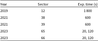
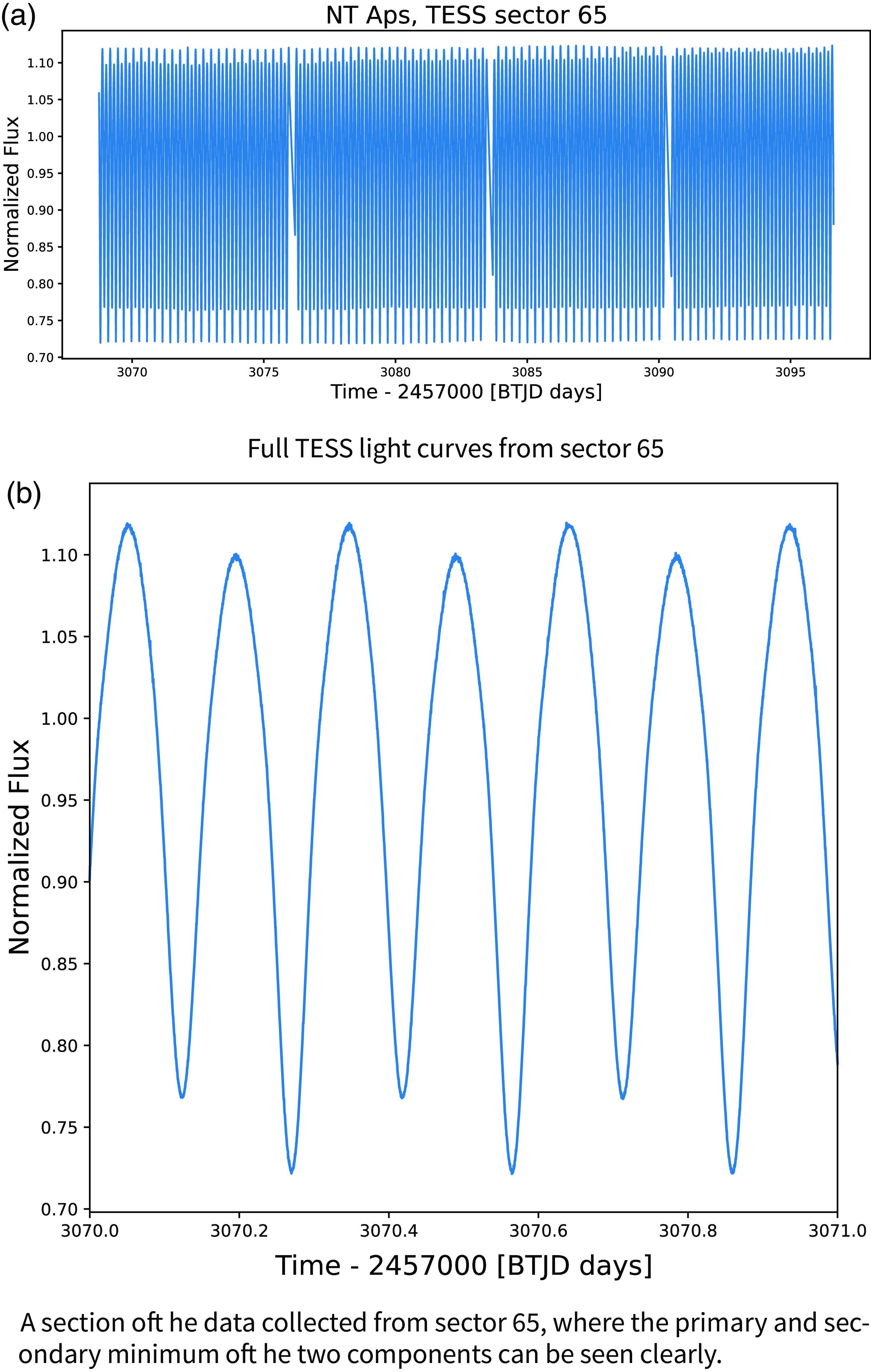
Figure 2. Light curve of NT Aps from TESS sector 65. The graphics are generated with Lightkurve.
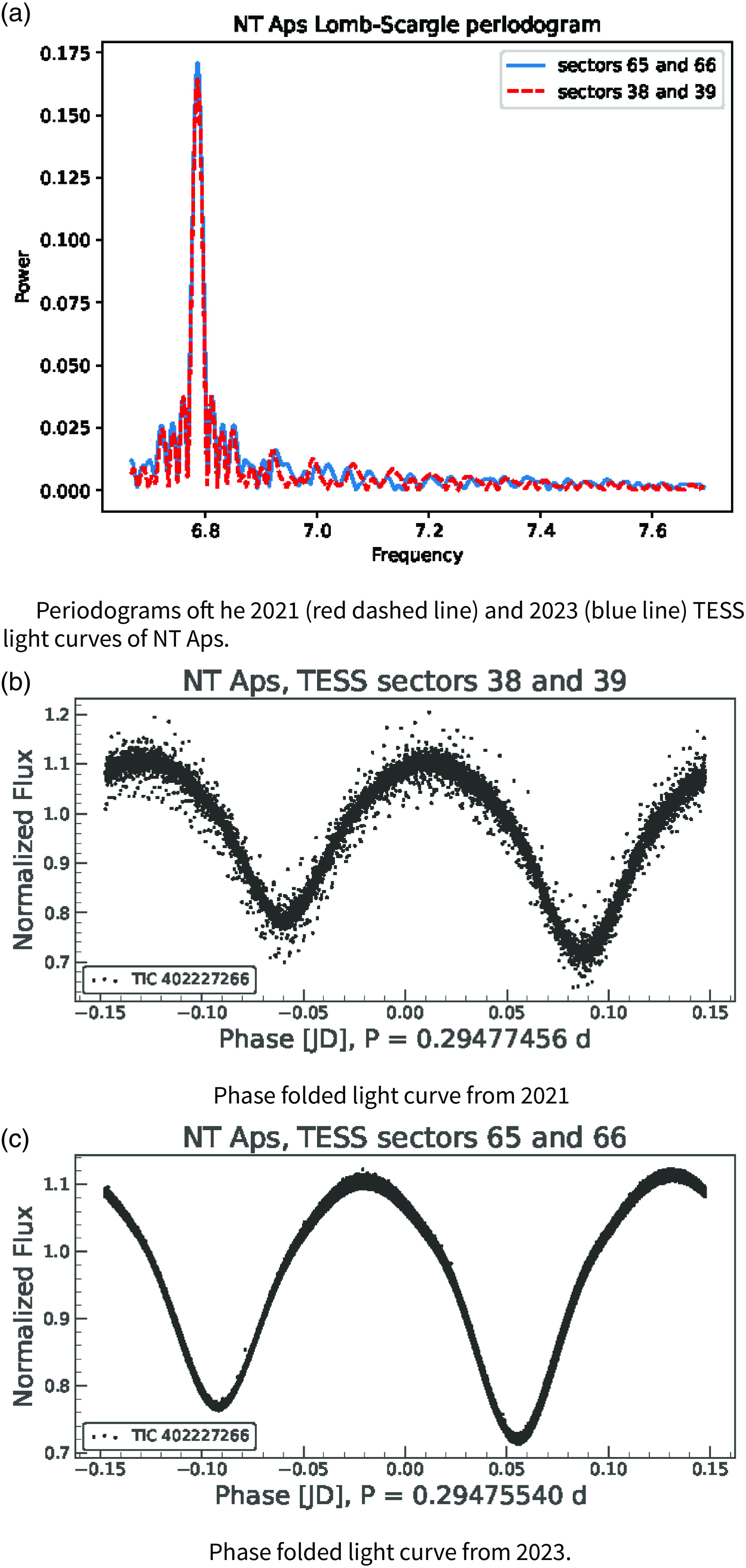
Figure 3. Periodograms and folded light curves of NT Aps for TESS observations in 2021 and 2023.
Plotting the phase-folded light curves showed that in both cases there are two minima with different depths that have been interpreted by the software as resulting from the same event, when in fact these are the primary and secondary minima of the binary. Thus, the actual period is twice the one obtained from the periodogram. For the two epochs and cadences, the periods of the system would be $P_1$
= 0.294775 d, and the
$P_1$
= 0.294775 d, and the $P_2$
= 0.294755 d, respectively. The phased light curves for the two epochs are shown in Fig. 3b and c, respectively. The difference between the two periods is less than two seconds, which contradicts the reported by Middleton (Reference Middleton2012) change in the period of 125 s per year. To check this, we also performed a Generalised Lomb-Scargle (GLS) analysis. The code can be found at: https://github.com/mzechmeister/GLS/commits?author=mzechmeister and is based on Zechmeister & Kürster (Reference Zechmeister and Kürster2009), & references therein. Using only 20 s cadence data from sectors 65 and 66, the GLS gives highest-power period of (0.14737425
$P_2$
= 0.294755 d, respectively. The phased light curves for the two epochs are shown in Fig. 3b and c, respectively. The difference between the two periods is less than two seconds, which contradicts the reported by Middleton (Reference Middleton2012) change in the period of 125 s per year. To check this, we also performed a Generalised Lomb-Scargle (GLS) analysis. The code can be found at: https://github.com/mzechmeister/GLS/commits?author=mzechmeister and is based on Zechmeister & Kürster (Reference Zechmeister and Kürster2009), & references therein. Using only 20 s cadence data from sectors 65 and 66, the GLS gives highest-power period of (0.14737425 $\pm 0.00000035$
) d, which is within 1 sec of the other value.
$\pm 0.00000035$
) d, which is within 1 sec of the other value.
There are several independent estimates for the period of the system in the literature. According to the GCVS catalogue (Samus et al. Reference Samus2015), it is 0.2947648000 days, according to Version 2 of Avvakumova et al. (Reference Avvakumova, Malkov and Kniazev2013) it is 0.2947599888 days, and the ASAS eclipsing binaries with RASS counterpart (Szczygiel et al. Reference Szczygiel, Socrates, Paczynski, Pojmanski and Pilecki2010) gives 0.294766 days. The difference between our results and those reported in the literature is on the magnitude of several seconds.
3.3 Long-term variation in the orbital period
From the TESS observations we have light curves in 5 sectors −12 in 2019, 38 and 39 in 2021, and 65 and 66 in 2023. To find the precise times of minima (in the Barycentric Julian Date (Barycentric Dynamical Time (BJDTDB)) we used a polynomial fit on subsets of the light curves around each minimum and time errors were obtained using the covariance matrices. As a result we extracted 163 primary and 163 secondary minima times from the 2023 data, 17 primary and 16 secondary minima from the 2021 data. However, due to the long cadence (30 min), the extracted times from the 2019 were with huge errors. To improve on these, we used a method, described in Wang et al. (Reference Wang, Jiang, Zhang, Zhao and Yu2017): assuming that the period does not change significantly in the span of three days, we took three such subsets from different parts of the light curve, computed their median points and shifted the data to one period around the median in each subset using the equation for the linear ephemeris: ${M = M_0 + P \times E}$
, where
${M = M_0 + P \times E}$
, where ${M_0}$
is the time of the median point, P is the period, and E is the number of cycles. An example of the original data and the resultant light curve is shown in Fig. 4. Thus, we obtained 3 primary and 3 secondary minima times with much higher precision. The same could not be done for the 2021 data due to high noise level in the fluxes. This is why we only used the minima with good fits. All the extracted minima times from TESS, together with minima times from the O-C gateway (http://var2.astro.cz/ocgate), and Richards et al. (Reference Richards, Axelsen, Blackford, Jenkins and Moriarty2021) are given in Table 3.
${M_0}$
is the time of the median point, P is the period, and E is the number of cycles. An example of the original data and the resultant light curve is shown in Fig. 4. Thus, we obtained 3 primary and 3 secondary minima times with much higher precision. The same could not be done for the 2021 data due to high noise level in the fluxes. This is why we only used the minima with good fits. All the extracted minima times from TESS, together with minima times from the O-C gateway (http://var2.astro.cz/ocgate), and Richards et al. (Reference Richards, Axelsen, Blackford, Jenkins and Moriarty2021) are given in Table 3.
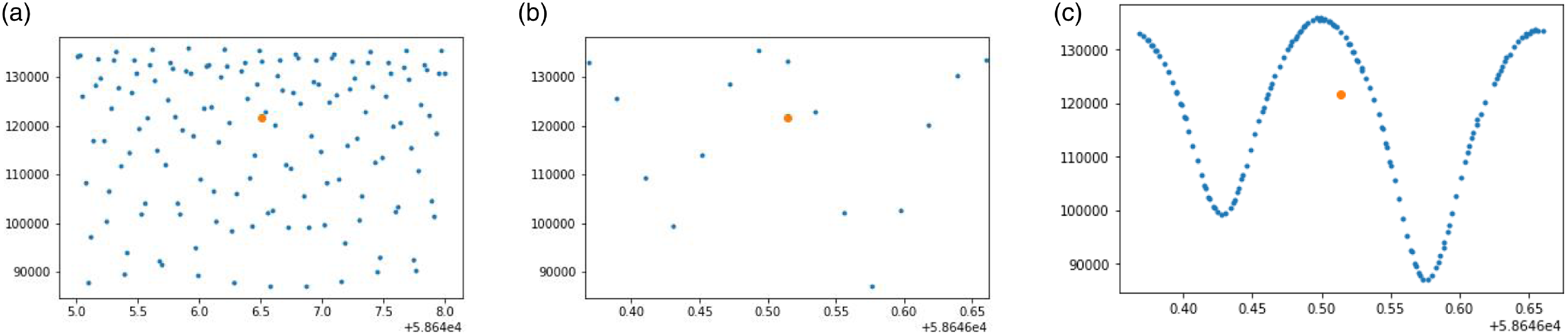
Figure 4. An example of using a three day segment of the NT Aps light curve from TESS in 2019 (shown in panel (a) together with its median in orange) to increase the data points to be used for the extraction of the minima. Panel (b) shows the original one period part around the median point. Panel (c) shows the result after the time-shift.
Table 3. Times of primary (column 1) and secondary (column 6) minima of NT Aps, their errors (columns 2 and 7, respectively), calculated epoch (columns 3 and 8), O-C value (columns 4 and 9). Columns 5 and 10 list the references, where 1: O-C gateway. Because we could not find the errors for these data, an arbitrary error of 0.02 was used. 2: Richards et al. (Reference Richards, Axelsen, Blackford, Jenkins and Moriarty2021). All times were converted to BJD. The full table is available in electronic format.
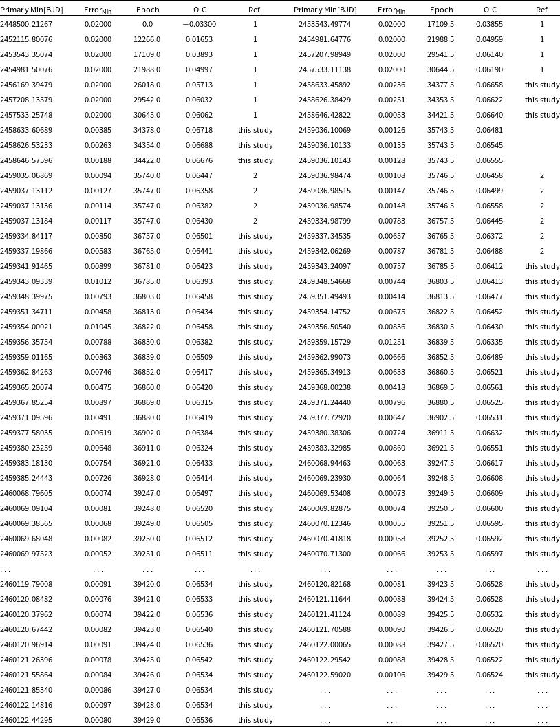
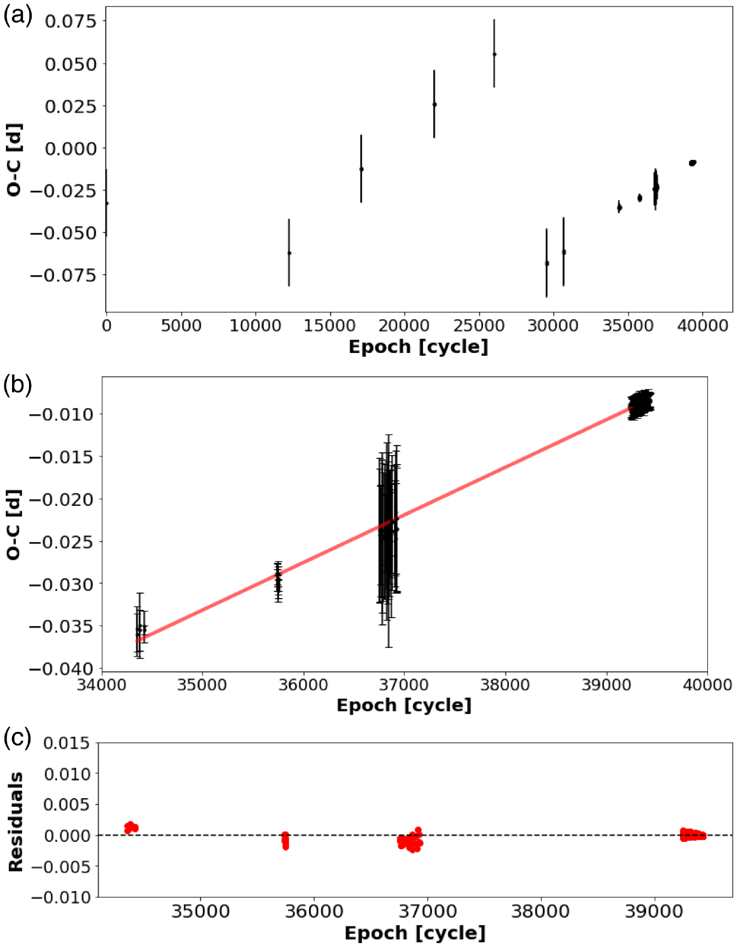
Figure 5. O-C diagram of NT Aps (a), linear fit of the 2019 to 2023 subset (b) and the residuals from the linear fit (c).
To examine the long term variations of the period we plotted the O-C diagram for the primary and secondary minima of NT Aps using the zero epoch from O-C gateway (http://var2.astro.cz/ocgate/) and the period, determined from the 2023 TESS data (Fig. 5a). As can be clearly seen there is a trend indicative of error in the period. To correct this, we fit the data subset from 2019 to 2023 with a linear fit using the Python emcee package (Foreman-Mackey et al. Reference Foreman-Mackey, Hogg, Lang and Goodman2013), where the values of $\delta$
P and
$\delta$
P and $\delta$
T were first calculated using the least-squares method, then used for the MCMC sampling with 100 walkers and 10 000 steps. The fit and its residuals are shown in Fig. 5b and c, respectively. As a result we obtained a correction in the period of:
$\delta$
T were first calculated using the least-squares method, then used for the MCMC sampling with 100 walkers and 10 000 steps. The fit and its residuals are shown in Fig. 5b and c, respectively. As a result we obtained a correction in the period of:
 \begin{align*}\delta P = (5.60338194_{-0.07180555}^{0.07108333}) \times 10^{-6} \textrm{(d)} \end{align*}

Figure 6. O-C diagram of NT Aps with quadratic fit (a) and residuals (b). The O-C is in days.
We re-plotted the O-C diagram with the updated period and fitted all the data with a quadratic function. The fit to the data and its residuals are shown in Fig. 6). The approach was the same as for the linear fit, but this time with 150 walkers and 30 000 steps. From this, for the coefficients of the fit ( $a\,x^2 + b\,x + c$
) we calculate:
$a\,x^2 + b\,x + c$
) we calculate:
 \begin{align*} a & = ({-}6.848 \pm 0.107) \times 10^{-11} \\b & = (5.191478 \pm 0.000001) \times 10^{-6}\\c & = -0.032650644849474 \pm 0.1025 \times 10^{-11} \end{align*}
Thus, using the equation for the quadrtatic epehmeris,
 \begin{align*}{M [BJD] = M_0 + P \times E + \frac{1}{2}\,\frac{dP}{dt}\times E^2},\end{align*}
we are able to calculate new ephemeris for the system:
 \begin{align*}M [BJD] = 2448500.2456657933 & {\, + \,0.29476620\,E} \\ & {-4.03697 \times 10^{-11}\,E^2}.\end{align*}
3.4 Orbital elements and parameters of the components
The radial velocities and light curves were analysed using the Eclipsing Binary Learning and Interactive System software package (ELISa) (Fedurco, Čokina, & Parimucha 2020; Čokina, Fedurco, & Parimucha 2021). The Python-only code aims to model stellar surfaces using Roche geometry, the triangulation process, and by doing synthetic observations and comparing them to the real ones to calculate the orbital parameters of the binary system. To generate synthetic observations of light curves or radial velocities, the package uses the Least Square Trust Region Reflective algorithm to do the first optimisation of system parameters. The results are then used as input parameters for the Markov-Chain Monte Carlo (MCMC) optimisation methods.
To fit the radial velocities of each component (obtained by processing the spectral observations from the two epochs) we used as inputs the system parameters obtained from the light curve modelling, but in parameter variation mode. The TESS observations for 2021 and 2023 concluded just before the beginning of our spectroscopic observations. Thus, to calculate the moments of the primary minima, we multiplied the most recent recorded primary minimum moment from TESS by the period of the system. This gives 2459333.815 for 2021 and 2460125.2397573 d for 2023. After several iterations of the least squares calculations we found the optimal solutions, which we subsequently use as input to the Monte Carlo modelling. Fig. 7 shows the model radial velocity curves, where the primary’s radial velocity is a blue continuous line, and the radial velocity for the second component is a red dashed line. The results from our spectroscopic analysis are shown using blue and red dots, respectively, with the errors shown as bars. We evaluated the least square fit both graphically and by determining the coefficient of determination. The coefficient for the 2023 data is 0.953805, whereas for the 2021 data it is 0.817424. This lower coefficient for 2021 is expected, since the quality of the data is poorer than that from 2023, as can be seen in Fig. 7.
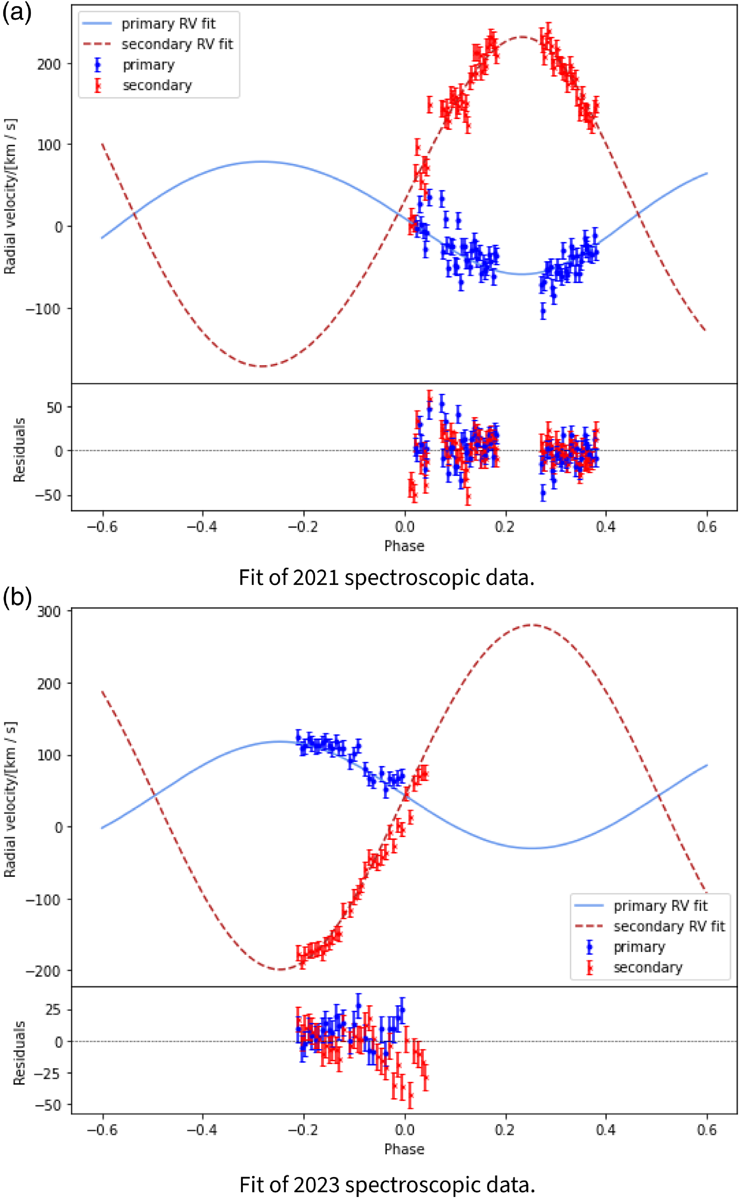
Figure 7. Radial velocity fit with least squares method of spectroscopic data.

Figure 8. Variations of the surface temperature for the two components of NT Aps.

Figure 9. The variations in surface acceleration in log g for the primary and secondary components are displayed in sections (a) and (b).
The solutions from the least squares computation (e = 0.09, ranging from 0.07 to 0.12; $\omega$
= 177 deg, ranging from 146 to 200; q = 0.33, ranging from 0.29 to 0.35; and
$\omega$
= 177 deg, ranging from 146 to 200; q = 0.33, ranging from 0.29 to 0.35; and $a\,\sin\!(i)$
= 1.57 R
$a\,\sin\!(i)$
= 1.57 R $\odot$
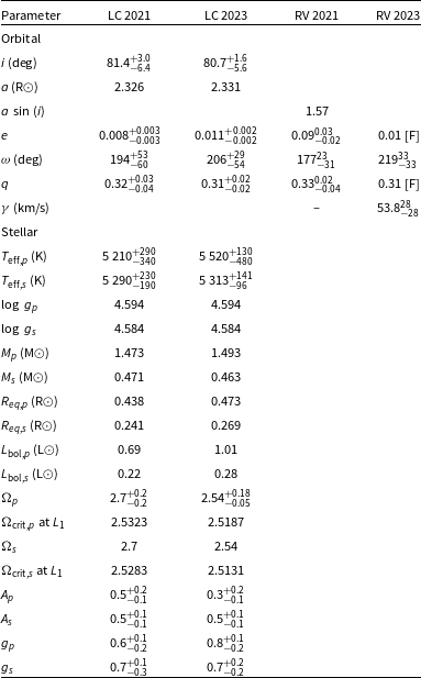
, ranging from 1.54 to 1.6) were used as inputs for the MCMC. The results are shown in Table 5. It is clear that there is a very good agreement between values of the parameters obtained from modelling the light curves (LC) and radial velocities (RV), as well as between data from different epochs, where the differences can be mostly attributed to the different quality/cadence of the data. The corner plots and the traces of the MCMC solutions for the LC and RV data can be seen in Figs. 11, 12, and 13 in Appendix A.
$\odot$
, ranging from 1.54 to 1.6) were used as inputs for the MCMC. The results are shown in Table 5. It is clear that there is a very good agreement between values of the parameters obtained from modelling the light curves (LC) and radial velocities (RV), as well as between data from different epochs, where the differences can be mostly attributed to the different quality/cadence of the data. The corner plots and the traces of the MCMC solutions for the LC and RV data can be seen in Figs. 11, 12, and 13 in Appendix A.
Using the parameters, calculated by the MCMC for the system for 2023, we can plot the surface temperature distribution (Fig. 8) and the variations of surface acceleration (Fig. 9), as well as the orbital positions of the components in a reference frame centred on the primary star and aligned with the orbital plane (Fig. 14, Appendix A), and the geometry of the system (Fig. 15, Appendix A).
For determining the parameters of the system, we used the shorter cadence TESS light curves from 2021 and 2023 and the period obtained from the GLS analysis (as a fixed input). To fit the light curves, we separated the two epochs and specified the TESS pass-band for the synthetic curve, setting the system as overcontact. We chose overcontact as the system type because, according to the Li et al. (Reference Li, Zhang, Han and Jiang2007) research on W UMa systems with varied periods, contact systems peak at around 0.35 days, which is the closest value to our system’s period. However, we also tested the setup for a detached system, which gave very similar results for the physical parameters, but did not properly model the light curve due to the different geometry.
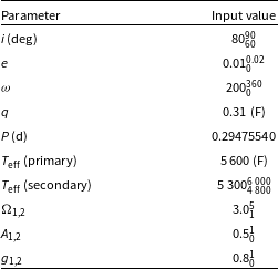
The ELISa package requires a number of additional input parameters for the synthetic light curve. These include the system’s inclination, eccentricity, mass ratio, periastron argument, semi-major axis, period, presence of third light, phase shift, and component characteristics as temperatures. All these are listed in Table 4. In the table, we have indicated if the parameter was set as a fixed [F] or variable one. For the variable parameters, we have given the variation range via subscript and superscript numbers.
Table 4. Least squares method synthetic LC input parameters for 2021 (sector 38, 10 min cadence) and 2023 (sector 66 with 20 s cadence) TESS data.
Some of the input parameters were also constrained based on the results from the RV fitting. The process was repeated until we achieved reasonable convergence of the parameters, present in both light curve and radial velocity models. The best light curve fits for the 2021 and 2023 TESS data are shown in Fig. 10. The blue colour represents the observational data, whereas the red colour represents the generated synthetic light curves. The fit for 2021 has a coefficient of determination of 0.97, while for 2023 it is 0.99.

Figure 10. Light curve fits using ELISa’s least squares method of TESS data, based on the parameters listed in Table 4.
Table 5. Parameters of the orbit and the system’s components (denoted with index p for primary and s for secondary) given by the MCMC method for the LC and the RV from 2021 and 2023. The listed orbital parameters are: inclination (i), semi-major axis a, projected semi-major axis ( $a\,\sin(i)$
), eccentricity (e), argument of periastron (
$a\,\sin(i)$
), eccentricity (e), argument of periastron ( $\omega$
); mass ratio (q), radial velocity of the system (
$\omega$
); mass ratio (q), radial velocity of the system ( $\gamma$
). The stellar parameters are: effective temperature (
$\gamma$
). The stellar parameters are: effective temperature ( $T_{\rm eff}$
), gravity (
$T_{\rm eff}$
), gravity ( $\log\,g$
), Mass (M), equivalent radius (
$\log\,g$
), Mass (M), equivalent radius ( $R_{eq}$
), bolometric luminosity (
$R_{eq}$
), bolometric luminosity ( $L_{\rm bol}$
), surface potential (
$L_{\rm bol}$
), surface potential ( $\Omega$
), critical potential (
$\Omega$
), critical potential ( $\Omega_{\rm crit}$
at L
$\Omega_{\rm crit}$
at L $_1$
) at the inner Lagrangian point L
$_1$
) at the inner Lagrangian point L $_1$
, albedo (A), gravity darkening factor (g).
$_1$
, albedo (A), gravity darkening factor (g).
As input for the MCMC simulations of the light curves of NT Aps, we used the parameters obtained from the least square method. Once again, we executed the analysis on a year-by-year basis, individually. During this step, each parameter is assigned as variable, but within a narrower range. We selected system mass ratio ranging from 0.2 to 0.4 and temperature range of 4 000–6 000 K for the primary component. Each simulation involves 200 steps and has a discretisation of 5. Discretisation here refers to the division of the surface into separate elements and the value is the spacing between points in degrees. The results for the orbital elements and the separate components are presented in Table 5. The sigma values as given as subscripts and superscripts.
The measured values for each parameter from the two epochs are within the error margins of each other. The observed differences can be attributed to the disparity in time resolution between the data collected in 2021 (10 min), and the data from 2023 (20 s). Although the two epochs have different resolutions, the analysis reveals similar values within the margin of error, thus confirming the consistency of the results.
From Table 5 it can be seen that the surface potentials for the stars exceed the critical potential at the inner Lagrangian point L $_1$
, which, according tho the ELISa handbookFootnote
a
is indicative of a contact binary. Using the values from 2023 for the surface and L
$_1$
, which, according tho the ELISa handbookFootnote
a
is indicative of a contact binary. Using the values from 2023 for the surface and L $_1$
critical potential,
$_1$
critical potential, $\Omega_{L_2}$
= 2.3178 (calculated with the applet of Leahy & Leahy Reference Leahy and Leahy2015), and the formula from Lucy & Wilson (Reference Lucy and Wilson1979), for the fill-out factor we get
$\Omega_{L_2}$
= 2.3178 (calculated with the applet of Leahy & Leahy Reference Leahy and Leahy2015), and the formula from Lucy & Wilson (Reference Lucy and Wilson1979), for the fill-out factor we get $f = 0.106$
, which again, points to a shallow contact system.
$f = 0.106$
, which again, points to a shallow contact system.
We also computed the orbital angular momentum ( $J_o$
) and placed the binary on the
$J_o$
) and placed the binary on the $\log J_o-\log_M$
diagram, presented by Eker et al. (Reference Eker, Demircan, Bilir and Karatas2006). The result (
$\log J_o-\log_M$
diagram, presented by Eker et al. (Reference Eker, Demircan, Bilir and Karatas2006). The result ( $\log J_o$
= 51.66 and
$\log J_o$
= 51.66 and $\log_M$
= 0.29), again, points to a contact system.
$\log_M$
= 0.29), again, points to a contact system.
3.5 Activity
We examined both the spectra and the photometric data for indications of activity. The residuals of the dynamic spectra (calculated by dividing each individual spectrum by the average one) show no signatures of flares and/or CMEs. The light curves from sectors 38,39,65 and 66 were inspected both visually and using the Altaipony (Ilin et al. Reference Ilin, Schmidt, Poppenhäger, Davenport, Kristiansen and Omohundro2021; Davenport Reference Davenport2016) procedures for detrending and flare finding. No candidates for flares were identified either way. We also modelled the light curves using ELISa with its option to include star spots. We ran the code using different locations, with latitudes ranging from 0 to 90 degrees, angular radii between 35 and 70 degrees, and a temperature factor of around 0.7 on the primary component. None of these runs produced a good fit to the data, that is, we can conclude that there are no large spots with these parameters on the primary component. However, the residuals from Fig. 10 indicate, that the existence of small spots on the surface of the components may be possible.
In addition, we searched the gPhoton database (Million et al. Reference Million2016a; Million et al. Reference Million, Fleming, Shiao and Loyd2016b) for GALEX ultraviolet observations of NT Aps. There are only two short observations ( $\approx$
96 s) in March and June 2007. The binary is brighter in the latter epoch by
$\approx$
96 s) in March and June 2007. The binary is brighter in the latter epoch by $\approx$
0.16 mag. This is most likely due to the rotation of the system. However, because of the short duration of the observations, we can neither confirm, nor exclude a contribution of activity induced flux to the brightening.
$\approx$
0.16 mag. This is most likely due to the rotation of the system. However, because of the short duration of the observations, we can neither confirm, nor exclude a contribution of activity induced flux to the brightening.
4. Discussion and conclusions
We modelled the light curves and radial velocities of NT Aps from two epochs – 2021 and 2023. However, in 2021, the quality of the spectroscopic observations was significantly poorer that that in 2023. In addition, the TESS photometry had cadence of 10 min, which led to a higher degree of dispersion in the phase folded light curve, compared to the one from 2023, which uses 20 s cadence data. For this reason, we adopt as more reliable the results, obtained from the modelling of the 2023 data and use these from now on.
Our model, compared to the one by Middleton (Reference Middleton2012) (the only other available in the literature for NT Aps) results in higher mass ratio ( $q =0.31$
to their 0.242) and inclination (
$q =0.31$
to their 0.242) and inclination ( $i = 80.7$
deg to their 71.9 deg) and significantly different temperatures for both components (
$i = 80.7$
deg to their 71.9 deg) and significantly different temperatures for both components ( $T_{{\rm eff},p} = 5\,520$
K, compared to 6 930 K and
$T_{{\rm eff},p} = 5\,520$
K, compared to 6 930 K and $T_{{\rm eff},s} = 5\,313$
K instead of 4 818 K). However, the light curve fit, produced by Middleton (Reference Middleton2012) does not describe the observations well, particularly the depth of the primary minimum (see Figures 4 and 5 in their paper). Note also that Middleton (Reference Middleton2012) only had ground-based photometry available for their study, whereas we use both high cadence, high precision space-based photometry and time series spectroscopy. Our atmospheric parameters are calculated based on spectral data and a new improved odf-values of Kurusz models by using ATLAS 12 code. Moreover the values of the effective temperature
$T_{{\rm eff},s} = 5\,313$
K instead of 4 818 K). However, the light curve fit, produced by Middleton (Reference Middleton2012) does not describe the observations well, particularly the depth of the primary minimum (see Figures 4 and 5 in their paper). Note also that Middleton (Reference Middleton2012) only had ground-based photometry available for their study, whereas we use both high cadence, high precision space-based photometry and time series spectroscopy. Our atmospheric parameters are calculated based on spectral data and a new improved odf-values of Kurusz models by using ATLAS 12 code. Moreover the values of the effective temperature $T_{\rm eff}$
and
$T_{\rm eff}$
and $\log g$
obtained by us match very well the ones, determined by GAIA DR3b (Gaia Collaboration et al. 2023).
$\log g$
obtained by us match very well the ones, determined by GAIA DR3b (Gaia Collaboration et al. 2023).
All of our analysis leads us to believe that we have improved the parameters of the system and its components in a more accurate way.
Based on the system and stellar parameters, we can conclude that NT Aps is a contact binary sharing a shallow common envelope (Lucy Reference Lucy1968b, Reference Lucy1968a), which is supported by the recent results of Ding et al. (Reference Ding, Song, Wang and Ji2024), who also clasify the system as a contact binary candidate based on analysis of TESS 120 sec light curves from sectors 65 and 66 only.
The light curve shows an EW-type variation (Qian et al. Reference Qian, Zhu, Liu, Zhang, Shi, He and Zhang2020, and refs. therein). Based on the study over 9 000 contact binaries, Qian et al. (Reference Qian, Zhu, Liu, Zhang, Shi, He and Zhang2020) obtained period distribution for these systems (see their Fig. 1) and constructed a heat map of the orbital period – effective temperature correlation (their Fig. 4). Our results show, that NT Aps lies very close to the peak of the period distribution (which is 0.31 d) and well within the region of normal EW-systems (i.e. neither marginal, nor deep contact system) on the period – temperature correlation.
Leitzinger et al. (Reference Leitzinger2020) estimated the flare and coronal mass ejection rate for NT Aps based on the X-ray luminosity of the target. They obtained an H $\alpha$
flare rate of 5.19 flares per day and extreme ultra-violet flare rate of 95.12 per day. They also estimated that NT Aps would show 0.2 coronal mass ejections a day. These are very large flare rates and indicate an active star. However, in our analysis we do not find evidence of strong magnetic activity in the time series spectra, nor in the broadband TESS light-curves. Our spectroscopic observations only cover couple of hours, so it is not too surprising that we do not see evidence of flaring activity in our EFOSC2 data. The same is true for the GALEX data, which covers even shorter time periods. Still, even if one cannot directly translate the flare rates of Leitzinger et al. (Reference Leitzinger2020) into the flare rate seen when using a broader wavelength band, like TESS data have, one would expect to see some flaring activity in the multi epoch photometry used in this study. It is clear that NT Aps is less active than what one would expect based on its X-ray luminosity and other stellar parameters. A possible explanation may be, as suggested by (Li et al. Reference Li, Zhang, Han and Jiang2007), that the magnetic activity level of W UMa systems is lower than that of similar but non-contact system or fast rotation single stars.
$\alpha$
flare rate of 5.19 flares per day and extreme ultra-violet flare rate of 95.12 per day. They also estimated that NT Aps would show 0.2 coronal mass ejections a day. These are very large flare rates and indicate an active star. However, in our analysis we do not find evidence of strong magnetic activity in the time series spectra, nor in the broadband TESS light-curves. Our spectroscopic observations only cover couple of hours, so it is not too surprising that we do not see evidence of flaring activity in our EFOSC2 data. The same is true for the GALEX data, which covers even shorter time periods. Still, even if one cannot directly translate the flare rates of Leitzinger et al. (Reference Leitzinger2020) into the flare rate seen when using a broader wavelength band, like TESS data have, one would expect to see some flaring activity in the multi epoch photometry used in this study. It is clear that NT Aps is less active than what one would expect based on its X-ray luminosity and other stellar parameters. A possible explanation may be, as suggested by (Li et al. Reference Li, Zhang, Han and Jiang2007), that the magnetic activity level of W UMa systems is lower than that of similar but non-contact system or fast rotation single stars.
In conclusion, here we present the first combined spectroscopic and photometric analysis of the southern eclipsing binary system NT Aps. Based on our results, the system is a short-period contact binary with a common envelope and/or close to equal temperatures, and an EW-type light curve. Neither the spectra, nor the photometry show signatures of activity, which suggests that the magnetic activity estimates published in the literature may need to be lowered, at least in the case of contact binaries.
Acknowledgement
This research made use of Lightkurve, a Python package for Kepler and TESS data analysis Lightkurve Collaboration et al. (2018). This paper includes data collected by the TESS mission, which are publicly available from the Mikulski Archive for Space Telescopes (MAST). Funding for the TESS mission is provided by the NASA’s Science Mission Directorate.
We are very grateful to Michal Cokina for their invaluable contributions to the recent discussion on ELISa: Eclipsing binary Learning and Interactive System (Čokina et al. 2021). This research has made use of the SIMBAD database, operated at CDS, Strasbourg, France. This work has made use of data from the European Space Agency (ESA) mission Gaia (https://www.cosmos.esa.int/gaia), processed by the Gaia Data Processing and Analysis Consortium (DPAC, https://www.cosmos.esa.int/web/gaia/dpac/consortium). Funding for the DPAC has been provided by national institutions, in particular the institutions participating in the Gaia Multilateral Agreement. Additional data analyses were done using ENVI version 4.8 (Exelis Visual Information Solutions, Boulder, Colorado).
We thank the anonymous referee for their constructive comments.
Data availability statement
Proprietary data available upon request from the corresponding author.
Funding statement
This work is supported by the Bulgarian NSF grant No.KP-06-N58/3 (2021). We also acknowledge support from ESO Science Support Discretionary Fund project SSDF21-06.
Competing interests
None
Appendix A. Supplementary materials
Appendix A.1. Radial velocities of the NT Aps components
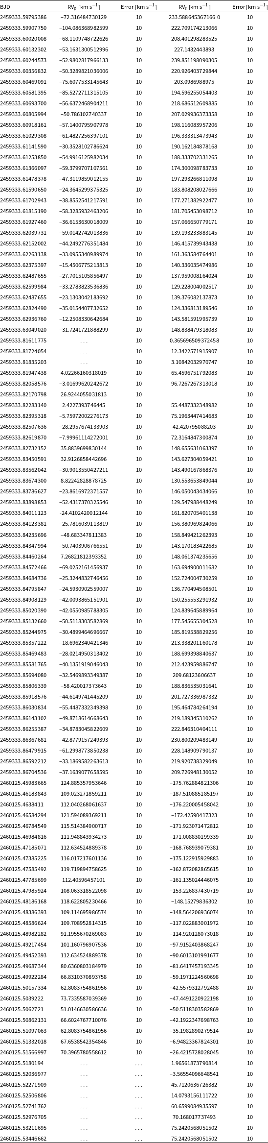
Table 6. Radial velocities of the primary (column 2) and secondary (column 4) component of the NT Aps system and their errors (column 3 and 5, respectively). Velocities are in km s $^{-1}$
and time is in BJD.
$^{-1}$
and time is in BJD.
Appendix A.2. Posterior distributions and traces for the results from ELISa’s MCMC runs

Figure 11. Traces of each parameter for 2023 TESS data.

Figure 12. Posterior distribution of MCMC sampling for light curve data from 2021 and 2023.

Figure 13. Posterior distribution of MCMC sampling for radial velocities data from 2021 and 2023.

Figure 14. 2D barycentric model of the orbits of the two components of NT Aps. The orbit of the primary component is in blue and the orbit of the secondary component is in orange.

Figure 15. Model of the NT Aps system with surface discretisation of the components.


 Open access