


1. Introduction
Locomotion of microorganisms and man-made microswimmers has been a subject of booming interest over the last decade due to its importance in many medical fields and biophysical processes, such as drug delivery, gut flora and red tide blooms (Nelson, Kaliakatsos & Abbott Reference Nelson, Kaliakatsos and Abbott2010; Li et al. Reference Li, Esteban-Fernández de Ávila, Gao, Zhang and Wang2017; Ishikawa & Pedley Reference Ishikawa and Pedley2023a ,Reference Ishikawa and Pedley b ). Swimming microorganisms inhabit a diverse range of complex fluid environments. Examples include a ciliate Tetrahymena inhabiting the mud, an infectious protozoa Trypanosoma entering the bloodstream and Helicobacter pylori in gastric mucus. Many biological fluids, such as blood or respiratory and gastric mucus, exhibit intricate rheological properties, including shear-thinning viscosity, viscoelasticity and viscoplasticity. While swimming in Newtonian fluids is well investigated (Lauga & Powers Reference Lauga and Powers2009; Lauga Reference Lauga2020; Ishikawa Reference Ishikawa2024), the hydrodynamics of swimming in these complex fluids is still evolving despite its fundamental biological and medical importance (Wu et al. Reference Wu, Chen, Mukasa, Pak and Gao2020; Spagnolie & Underhill Reference Spagnolie and Underhill2023).
To date, several studies have explored the hydrodynamics of microswimmers in shear-thinning fluids (Datt et al. Reference Datt, Zhu, Elfring and Pak2015; Elfring & Lauga Reference Elfring and Lauga2015; Nganguia et al. Reference Nganguia, Pietrzyk and Pak2017; Pietrzyk et al. Reference Pietrzyk, Nganguia, Datt, Zhu, Elfring and Pak2019; van Gogh et al. Reference van Gogh, Demir, Palaniappan and Pak2022), viscoelastic fluids (Zhu, Lauga & Brandt Reference Zhu, Lauga and Brandt2012; Binagia et al. Reference Binagia, Phoa, Housiadas and Shaqfeh2020; Housiadas, Binagia & Shaqfeh Reference Housiadas, Binagia and Shaqfeh2021; Li, Lauga & Ardekani Reference Li, Lauga and Ardekani2021; Ouyang et al. Reference Ouyang, Lin, Lin, Phan-Thien and Zhu2023), porous media (Nganguia & Pak Reference Nganguia and Pak2018; Nganguia et al. Reference Nganguia, Zhu, Palaniappan and Pak2020; Demir et al. Reference Demir, van Gogh, Palaniappan and Nganguia2024), blood suspensions (Wu et al. Reference Wu, Omori and Ishikawa2024a ,Reference Wu, Omori and Ishikawa b ), fluids with non-uniform viscosity (Eastham & Shoele Reference Eastham and Shoele2020; Gong, Shaik & Elfring Reference Gong, Shaik and Elfring2024), as well as viscoplastic fluids (Eastham, Mohammadigoushki & Shoele Reference Eastham, Mohammadigoushki and Shoele2022). The combination of these results suggests that non-Newtonian rheology has a profound impact on the locomotion of microswimmers.
The viscoplastic fluids exhibit yield stress, beyond which they flow viscously, while at lower stress levels they behave as solids. A typical example of swimming in a viscoplastic fluid is H. pylori bacterium moving through dense, gel-like gastric mucus (Celli et al. Reference Celli2009; Mirbagheri & Fu Reference Mirbagheri and Fu2016). Experimental studies of locomotion in viscoplastic fluids have observed that helical and undulatory swimmers are able to swim faster than in a Newtonian fluid (Dorgan, Law & Rouse Reference Dorgan, Law and Rouse2013; Kudrolli & Ramirez Reference Kudrolli and Ramirez2019; Nazari, Shoele & Mohammadigoushki Reference Nazari, Shoele and Mohammadigoushki2023). Most previous numerical studies on swimming in viscoplastic fluids have been confined to two dimensions (Hewitt & Balmforth Reference Hewitt and Balmforth2017; Supekar, Hewitt & Balmforth Reference Supekar, Hewitt and Balmforth2020) or slender bodies (Hewitt & Balmforth Reference Hewitt and Balmforth2018). Recently, Hewitt (Reference Hewitt2024) reviewed the studies of locomotion through a viscoplastic fluid for cylindrical filamentary bodies.
In order to understand the dynamics of swimming microorganisms, several fluid dynamical models for low Reynolds number environments have been proposed. A simplified ciliate model known as the ‘squirmer’ was first introduced by Lighthill (Reference Lighthill1952) and then generalised by Blake (Reference Blake1971). Keller & Wu (Reference Keller and Wu1977) built on the model by extending the squirmer to be prolate ellipsoidal. Their model has been extended to include a force-dipole mode (Ishimoto & Gaffney Reference Ishimoto and Gaffney2013; Theers et al. Reference Theers, Westphal, Gompper and Winkler2016; van Gogh et al. Reference van Gogh, Demir, Palaniappan and Pak2022). The squirmer model has therefore become a popular generic locomotion model for various problems such as hydrodynamic interactions (Ishikawa et al. Reference Ishikawa, Simmonds and Pedley2006, Reference Ishikawa, Pedley, Drescher and Goldstein2020) and active suspensions (Ishikawa, Brumley & Pedley Reference Ishikawa, Brumley and Pedley2021; Qi et al. Reference Qi, Westphal, Gompper and Winkler2022; Zantop & Stark Reference Zantop and Stark2022).
Eastham et al. (Reference Eastham, Mohammadigoushki and Shoele2022) employed the spherical squirmer model to investigate how fluid plasticity affects locomotion performance in a Bingham viscoplastic fluid. This study found that a spherical squirmer in a Bingham fluid experiences reduced swimming speed and increased energy dissipation as the Bingham number increases. Nevertheless, the swimming efficiency reaches a maximum at a moderate Bingham number. Swimming in viscoplastic fluids also has some similarities with swimming in confinement, as the viscous fluid region is bounded by the solid region. Reigh & Lauga (Reference Reigh and Lauga2017) and Nganguia et al. (Reference Nganguia, Zhu, Palaniappan and Pak2020) studied the dynamics of a spherical squirmer encapsulated in a spherical droplet by theory and simulation, and found that the swimming speed depends on the size ratio between the droplet and the squirmer. Aymen et al. (Reference Aymen, Palaniappan, Demir and Nganguia2023) and Della-Giustina, Nganguia & Demir (Reference Della-Giustina, Nganguia and Demir2023) further extended the model to include swimmer shape and medium heterogeneity. These studies consistently reported that the swimming speed of a neutral squirmer increases as the size ratio between the closed domain and the squirmer increases, unless the ratio is too small.
The flow field generated by the microswimmers also affects the diffusion properties of the suspension, which are crucial in biological processes such as reproduction, colonisation and infection. As the microorganisms mix the fluid as they swim, they enhance the diffusion of chemicals and tracers (Katija & Dabiri Reference Katija and Dabiri2009; Thiffeault & Childress Reference Thiffeault and Childress2010; Lin, Thiffeault & Childress Reference Lin, Thiffeault and Childress2011; Nordanger, Morozov & Stenhammar Reference Nordanger, Morozov and Stenhammar2023). The enhanced diffusion was first measured experimentally by Wu & Libchaber (Reference Wu and Libchaber2000) in a suspension of Escherichia coli bacteria. Experiments have shown that the scaling between the enhanced diffusion due to swimmer activity and swimmer volume fraction is linear at low volume fractions (Leptos et al. Reference Leptos, Guasto, Gollub, Pesci and Goldstein2009; Jepson et al. Reference Jepson, Martinez, Schwarz-Linek, Morozov and Poon2013; Kasyap, Koch & Wu Reference Kasyap, Koch and Wu2014). Such enhanced diffusion in dilute or semi-dilute suspensions of microswimmers is also reported by simulations and theoretical studies (Underhill, Hernandez-Ortiz & Graham Reference Underhill, Hernandez-Ortiz and Graham2008; Ishikawa, Locsei & Pedley Reference Ishikawa, Locsei and Pedley2010; Kurtuldu et al. Reference Kurtuldu, Guasto, Johnson and Gollub2011; Miño et al. Reference Miño, Dunstan, Rousselet, Clément and Soto2013). Ishikawa et al. (Reference Ishikawa, Locsei and Pedley2010) showed that the flow-induced diffusivity is proportional to the volume fraction of squirmers in the semi-dilute regime. Studies have also been carried out on tracer displacements induced by individual swimmers (Thiffeault & Childress Reference Thiffeault and Childress2010; Lin et al. Reference Lin, Thiffeault and Childress2011; Pushkin, Shum & Yeomans Reference Pushkin, Shum and Yeomans2013; Mathijssen, Pushkin & Yeomans Reference Mathijssen, Pushkin and Yeomans2015; Mueller & Thiffeault Reference Mueller and Thiffeault2017). These studies provide a fundamental understanding of how individual swimming motions contribute to the overall diffusive behaviour in a suspension. Squirmers swimming in a viscoplastic fluid can only displace fluid particles within the yielded region, while fluid particles outside the yielded region remain stationary. This should have important implications for the swimmer-induced transport of chemicals and tracers. However, to the best of the authors’ knowledge, our current understanding of swimmer-induced diffusion rests mainly on Newtonian fluids, and the effect of viscoplasticity is unexplored.
Furthermore, the effect of the swimmer’s body shape on swimming performance can be qualitatively different in Newtonian and non-Newtonian fluids. Recent studies have reported that the body shape plays a significant role in the locomotion of microswimmers through complex fluids (Eastham & Shoele Reference Eastham and Shoele2020; van Gogh et al. Reference van Gogh, Demir, Palaniappan and Pak2022; Demir et al. Reference Demir, van Gogh, Palaniappan and Nganguia2024; Gong et al. Reference Gong, Shaik and Elfring2024; Ouyang et al. Reference Ouyang, Liu, Lin and Lin2024). van Gogh et al. (Reference van Gogh, Demir, Palaniappan and Pak2022) demonstrated that an elongated ellipsoidal microswimmer can swim faster and more effectively in a shear-thinning fluid than in a Newtonian fluid. Similarly, Demir et al. (Reference Demir, van Gogh, Palaniappan and Nganguia2024) showed that an ellipsoidal microswimmer always propels faster, consumes less energy and is more efficient than a spherical microswimmer in either a homogeneous fluid or a heterogeneous medium. When swimming in a fluid with linearly varying viscosity, Gong et al. (Reference Gong, Shaik and Elfring2024) found that the effect of viscosity gradients on power dissipation and efficiency diminishes as the slenderness of the swimmer increases.
Nevertheless, the effect of body shape on locomotion in viscoplastic fluids remains unclear. In this study, we employ the spheroidal squirmer model to probe the role of body shape in swimming in a Bingham viscoplastic environment. The results reveal key features that are distinct from those obtained using the spherical squirmer model, suggesting that both biological and artificial microswimmers could potentially optimise their geometric shape or swimming mode to enhance swimming performance in viscoplastic environments. In addition, this study investigates the influence of viscoplasticity on swimmer-induced diffusion in a dilute suspension. The plasticity enforces the velocity far from the swimmer to be zero, thus breaking the assumptions used in Newtonian fluids, such as the velocity perturbation induced by a force-free swimmer decays with the square of the distance. Swimmer-induced diffusion in a plastic fluid has not been reported before, so new insights can be gained.
The paper is structured as follows. We formulate the problem in § 2 by introducing the squirmer model and the governing equations, and discuss the numerical method. We investigate swimming in a viscoplastic fluid in § 3. The effects of the swimmer shape, the polar and swirling squirming velocities and the Bingham number on the propulsion behaviour are examined. The differences in the propulsion speed across various aspect ratios is explained in terms of forces acting on the body. In § 4, we discuss the squirmer-induced tracer diffusion in a dilute suspension. The motion of tracers in a plastic fluid is restricted to the vicinity of the squirmer. Since the outer region can be regarded as solid, the Brownian motion of the tracers can be ignored. By assuming diluteness, the tracer particles only move when a swimmer comes close and otherwise remain stationary. Moreover, if an isotropic suspension is assumed, where the orientation of the squirmers is isotropic, the tracer exhibits a three-dimensional random walk, taking steps only when the squirmer comes close. The diffusion coefficient is derived under these assumptions and the effects of the swimmer shape, the swimming modes and the Bingham number on the diffusivity are discussed. Finally, we conclude this study in § 5.
2. Basic equations and numerical methods
2.1. The squirmer model
We consider an ellipsoidal microswimmer propelling through a viscoplastic fluid, as illustrated in figure 1(a). The swimmer has the aspect ratio $a_r = b_x/b_z$
, with semi-major axis
$a_r = b_x/b_z$
, with semi-major axis $b_x$
and semi-minor axis
$b_x$
and semi-minor axis $b_z$
, as shown in figure 1(b). We denote half of the focal length by
$b_z$
, as shown in figure 1(b). We denote half of the focal length by $c = \sqrt {b_x^2 - b_z^2}$
, which yields the eccentricity
$c = \sqrt {b_x^2 - b_z^2}$
, which yields the eccentricity $e=c/b_x$
(
$e=c/b_x$
( $0 \leqslant e \lt 1$
, with
$0 \leqslant e \lt 1$
, with $e\,{=}\,0$
describing a sphere). The prolate spheroidal coordinate system (
$e\,{=}\,0$
describing a sphere). The prolate spheroidal coordinate system ( $\zeta, \tau, \varphi$
) is related to the body-fixed Cartesian coordinates
$\zeta, \tau, \varphi$
) is related to the body-fixed Cartesian coordinates $(x^{\prime},y^{\prime},z^{\prime})$
via (Dassios, Hadjinicolaou & Payatakes Reference Dassios, Hadjinicolaou and Payatakes1994)
$(x^{\prime},y^{\prime},z^{\prime})$
via (Dassios, Hadjinicolaou & Payatakes Reference Dassios, Hadjinicolaou and Payatakes1994)
 \begin{equation} \zeta = \frac {1}{{2c}}\left ( {\sqrt {{{(x^{\prime} + c)}^2}+{y^{\prime 2}} + {z^{\prime 2}}} - \sqrt {{{(x^{\prime} - c)}^2}+{y^{\prime 2}} + {z^{\prime 2}}} } \right), \end{equation}
 \begin{equation} \tau = \frac {1}{{2c}}\left ( {\sqrt {{{(x^{\prime} + c)}^2}+{y^{\prime 2}} + {z^{\prime 2}}} + \sqrt {{{(x^{\prime} - c)}^2}+{y^{\prime 2}} + {z^{\prime 2}}} } \right), \end{equation}
 \begin{equation} \varphi = \arctan \left ( {\frac {y^{\prime}}{z^{\prime}}} \right). \end{equation}

Figure 1. (a) Computational set-up of an ellipsoidal microswimmer in a Bingham fluid environment. (b) Sketch of an ellipsoidal microswimmer, where $b_x$
and
$b_x$
and $b_z$
are the semi-major and semi-minor axes of the ellipsoid. Here,
$b_z$
are the semi-major and semi-minor axes of the ellipsoid. Here, $r_{eq}=(b_xb_z^2)^{1/3}$
refers to the equivalent radius of the ellipsoidal microswimmer.
$r_{eq}=(b_xb_z^2)^{1/3}$
refers to the equivalent radius of the ellipsoidal microswimmer.
In the equations, $-1 \leqslant \zeta \leqslant 1$
,
$-1 \leqslant \zeta \leqslant 1$
, $1 \leqslant \tau$
and
$1 \leqslant \tau$
and $0 \leqslant \varphi \lt 2\pi$
. All points with
$0 \leqslant \varphi \lt 2\pi$
. All points with $\tau = \tau _0 \equiv e^{-1}$
(i.e.
$\tau = \tau _0 \equiv e^{-1}$
(i.e. ${x^{\prime 2}}/b_x^2 + ( {{{y^{\prime}}^2} + {{z^{\prime}}^2}})/b_z^2 = 1$
) lie on the ellipsoid’s surface.
${x^{\prime 2}}/b_x^2 + ( {{{y^{\prime}}^2} + {{z^{\prime}}^2}})/b_z^2 = 1$
) lie on the ellipsoid’s surface.
The microswimmer is modelled as a spheroidal squirmer in this research. In the squirmer model, the propulsion is generated by imposing surface squirming velocities. The surface velocity is assumed to be tangential, steady and axisymmetric. The general form of the surface velocity with an azimuthal component is expressed as (Pak & Lauga Reference Pak and Lauga2014; Pedley, Brumley & Goldstein Reference Pedley, Brumley and Goldstein2016)
 \begin{equation} \boldsymbol{u}_{sq}=-\sum _{n=1}^{\infty } \frac {2 B_n}{n(n+1)} P_n^{\prime }(\boldsymbol{p} \cdot \boldsymbol{n}) \boldsymbol{p} \cdot (\unicode{x1D644}-\boldsymbol{n n})-\sum _{n=1}^{\infty } C_n P_n^{\prime }(\boldsymbol{p} \cdot \boldsymbol{n}) \left | \boldsymbol{p} \cdot (\unicode{x1D644}-\boldsymbol{n n})\right | \boldsymbol{t}, \end{equation}
where ${\boldsymbol{p}}=\boldsymbol{e}_p$
is the unit orientation vector,
${\boldsymbol{p}}=\boldsymbol{e}_p$
is the unit orientation vector, $\boldsymbol{n}=\boldsymbol{e}_\tau$
is the unit normal vector and
$\boldsymbol{n}=\boldsymbol{e}_\tau$
is the unit normal vector and $\boldsymbol{t}=\boldsymbol{e}_\varphi$
is the unit azimuthal tangent vector;
$\boldsymbol{t}=\boldsymbol{e}_\varphi$
is the unit azimuthal tangent vector; $\unicode{x1D644}$
is the unit tensor and
$\unicode{x1D644}$
is the unit tensor and $P^{\prime}_n$
is the derivative of the
$P^{\prime}_n$
is the derivative of the $n$
th-order Legendre polynomial. The coefficients
$n$
th-order Legendre polynomial. The coefficients $B_n$
and
$B_n$
and $C_n$
are often called polar modes and azimuthal (or swirling) modes, respectively. Typically, only the first two polar squirming modes (
$C_n$
are often called polar modes and azimuthal (or swirling) modes, respectively. Typically, only the first two polar squirming modes ( $B_1$
and
$B_1$
and $B_2$
) are considered. The first polar mode
$B_2$
) are considered. The first polar mode $B_1$
determines the swimming speed
$B_1$
determines the swimming speed $U_N$
in an infinite Newtonian fluid in the Stokes flow regime as (Keller & Wu Reference Keller and Wu1977; Theers et al. Reference Theers, Westphal, Gompper and Winkler2016)
$U_N$
in an infinite Newtonian fluid in the Stokes flow regime as (Keller & Wu Reference Keller and Wu1977; Theers et al. Reference Theers, Westphal, Gompper and Winkler2016)
 \begin{equation} U_N=B_1 \tau _0\left(\tau _0-\left(\tau _0^2-1\right) \operatorname {coth}^{-1} \tau _0\right)\kern-2.5pt. \end{equation}
The swimming speed of a spherical swimmer is recovered for the spherical limit ( ${\tau _0} \to \infty$
) as
${\tau _0} \to \infty$
) as $U_N=2B_1/3$
. Therefore,
$U_N=2B_1/3$
. Therefore, $B_1$
is chosen as the characteristic velocity scale. The second polar mode
$B_1$
is chosen as the characteristic velocity scale. The second polar mode $B_2$
regulates the strength of a force dipole, i.e. the stresslet, in an infinite Newtonian fluid (Ishikawa, Simmonds & Pedley Reference Ishikawa, Simmonds and Pedley2006). Recently, researchers have started to consider the effect of higher-order polar modes (Datt et al. Reference Datt, Zhu, Elfring and Pak2015; De Corato & D’Avino Reference De Corato and D’Avino2017; Pietrzyk et al. Reference Pietrzyk, Nganguia, Datt, Zhu, Elfring and Pak2019) or the azimuthal swirling modes (Pak & Lauga Reference Pak and Lauga2014; Pedley et al. Reference Pedley, Brumley and Goldstein2016; Binagia et al. Reference Binagia, Phoa, Housiadas and Shaqfeh2020; Fortune et al. Reference Fortune, Worley, Sendova-Franks, Franks, Leptos, Lauga and Goldstein2021) on the swimming of spherical squirmers. Nevertheless, the effect of the azimuthal modes on the swimming dynamics of non-spherical squirmers in a complex fluid has not been reported.
$B_2$
regulates the strength of a force dipole, i.e. the stresslet, in an infinite Newtonian fluid (Ishikawa, Simmonds & Pedley Reference Ishikawa, Simmonds and Pedley2006). Recently, researchers have started to consider the effect of higher-order polar modes (Datt et al. Reference Datt, Zhu, Elfring and Pak2015; De Corato & D’Avino Reference De Corato and D’Avino2017; Pietrzyk et al. Reference Pietrzyk, Nganguia, Datt, Zhu, Elfring and Pak2019) or the azimuthal swirling modes (Pak & Lauga Reference Pak and Lauga2014; Pedley et al. Reference Pedley, Brumley and Goldstein2016; Binagia et al. Reference Binagia, Phoa, Housiadas and Shaqfeh2020; Fortune et al. Reference Fortune, Worley, Sendova-Franks, Franks, Leptos, Lauga and Goldstein2021) on the swimming of spherical squirmers. Nevertheless, the effect of the azimuthal modes on the swimming dynamics of non-spherical squirmers in a complex fluid has not been reported.
We consider the prescribed surface velocity (2.4) with the first two polar modes ( $B_1$
and
$B_1$
and $B_2$
) and the second azimuthal mode (
$B_2$
) and the second azimuthal mode ( $C_2$
) as being non-zero, then it is simplified as
$C_2$
) as being non-zero, then it is simplified as
 \begin{align} {{\boldsymbol{u}}_{{{sq}}}} & = - {B_1} ( {{{\boldsymbol{e}}_\zeta }\cdot {{\boldsymbol{e}}_p}} ){{\boldsymbol{e}}_\zeta } - {B_2}\zeta ( {{{\boldsymbol{e}}_\zeta }\cdot {{\boldsymbol{e}}_p}} ){{\boldsymbol{e}}_\zeta } - 3{C_2}\zeta ( {{{\boldsymbol{e}}_\zeta } \cdot {{\boldsymbol{e}}_p}} ){{\boldsymbol{e}}_\varphi } \nonumber\\& =-B_1 \tau _0 (1-\zeta ^2)^{\frac {1}{2}} (\tau _0^2-\zeta ^2)^{-\frac {1}{2}} [(1+\beta \zeta) \boldsymbol{e}_\zeta +3 \chi \zeta \boldsymbol{e}_{\varphi }]. \end{align}
The ratios $\beta = B_2/B_1$
and
$\beta = B_2/B_1$
and $\chi =C_2/B_1$
represent the squirmer’s dipolarity and chirality, respectively. Dipolarity
$\chi =C_2/B_1$
represent the squirmer’s dipolarity and chirality, respectively. Dipolarity $\beta$
helps in categorising the types of microswimmer as pusher (
$\beta$
helps in categorising the types of microswimmer as pusher ( $\beta\,{\lt}\,0$
, e.g. E. coli), puller (
$\beta\,{\lt}\,0$
, e.g. E. coli), puller ( $\beta \gt 0$
, e.g. Chlamydomonas) and neutral (
$\beta \gt 0$
, e.g. Chlamydomonas) and neutral ( $\beta = 0$
, e.g. Volvox) types, while chirality
$\beta = 0$
, e.g. Volvox) types, while chirality $\chi$
represents the intensity of a microswimmer with rotating flagella and a counter-rotating body (Pedley et al. Reference Pedley, Brumley and Goldstein2016; Binagia et al. Reference Binagia, Phoa, Housiadas and Shaqfeh2020; Fadda, Molina & Yamamoto Reference Fadda, Molina and Yamamoto2020). We refer to the squirmer with
$\chi$
represents the intensity of a microswimmer with rotating flagella and a counter-rotating body (Pedley et al. Reference Pedley, Brumley and Goldstein2016; Binagia et al. Reference Binagia, Phoa, Housiadas and Shaqfeh2020; Fadda, Molina & Yamamoto Reference Fadda, Molina and Yamamoto2020). We refer to the squirmer with $\chi \ne 0$
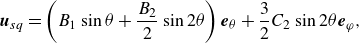
as a swirling squirmer. Note that the surface velocity for spherical squirmer is recovered in the spherical limit (
$\chi \ne 0$
as a swirling squirmer. Note that the surface velocity for spherical squirmer is recovered in the spherical limit ( $\zeta \rightarrow \cos \theta$
) (Housiadas et al. Reference Housiadas, Binagia and Shaqfeh2021; Kobayashi, Molina & Yamamoto Reference Kobayashi, Molina and Yamamoto2024) as
$\zeta \rightarrow \cos \theta$
) (Housiadas et al. Reference Housiadas, Binagia and Shaqfeh2021; Kobayashi, Molina & Yamamoto Reference Kobayashi, Molina and Yamamoto2024) as
 \begin{equation} {{\boldsymbol{u}}_{sq}} = \left ( {{B_1}\sin \theta + \frac {{{B_2}}}{2}\sin 2\theta } \right){{\boldsymbol{e}}_\theta } + \frac {3}{2}{C_2}\sin 2\theta {{\boldsymbol{e}}_\varphi }, \end{equation}
where $\theta =\arccos (\boldsymbol{p} \cdot \boldsymbol{r} / r)$
represents the polar angle between the position vector
$\theta =\arccos (\boldsymbol{p} \cdot \boldsymbol{r} / r)$
represents the polar angle between the position vector $\boldsymbol{r}$
and the swimming direction
$\boldsymbol{r}$
and the swimming direction $\boldsymbol{p}$
, while
$\boldsymbol{p}$
, while ${\boldsymbol{e}}_\theta$
is the unit tangent vector along the
${\boldsymbol{e}}_\theta$
is the unit tangent vector along the $\theta$
direction. In the present study, we investigate three types of swimmers: neutral swimmers (
$\theta$
direction. In the present study, we investigate three types of swimmers: neutral swimmers ( $\beta =\chi =0$
), pullers or pushers (
$\beta =\chi =0$
), pullers or pushers ( $\beta \ne 0,\chi =0$
) and neutral swirling swimmers (
$\beta \ne 0,\chi =0$
) and neutral swirling swimmers ( $\beta =0,\chi \ne 0$
).
$\beta =0,\chi \ne 0$
).
2.2. Basic equations
The locomotion of a squirmer through a viscoplastic fluid is simulated by the direct forcing/fictitious domain method (Yu & Shao Reference Yu and Shao2007; Yu & Wachs Reference Yu and Wachs2007). Let $\Omega$
and
$\Omega$
and $P$
represent the entire domain and the domain occupied by the squirmer, respectively (
$P$
represent the entire domain and the domain occupied by the squirmer, respectively ( $P\,{\subset}\,\Omega$
);
$P\,{\subset}\,\Omega$
); $P$
is bounded by the squirmer surface
$P$
is bounded by the squirmer surface $S$
. The governing equations are written as
$S$
. The governing equations are written as
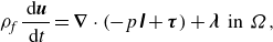 \begin{equation} \rho _{\!f} \frac {\mathrm{\ d} \boldsymbol{u}}{\mathrm{\ d} t}= \boldsymbol{\nabla } \cdot \left (-p \unicode{x1D644}+\boldsymbol{\tau }\right) + \boldsymbol{\lambda }\;\; {\textrm {in}} \;\;{\Omega }, \end{equation}
 \begin{equation} \boldsymbol{u}=(\boldsymbol{U}+\boldsymbol{\omega } \times \boldsymbol{r})+\boldsymbol{u}_{sq}\;\; {\textrm {in}} \;\;{S}, \end{equation}
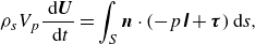 \begin{equation} \rho _s V_p \frac {\mathrm{\ d} \boldsymbol{U}}{\mathrm{\ d} t}=\int _S \boldsymbol{n} \cdot \left (-p \unicode{x1D644}+\boldsymbol{\tau }\right) \mathrm{d} s, \end{equation}
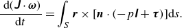 \begin{equation} \frac {\mathrm{\ d}(\unicode{x1D645} \cdot {\boldsymbol{\omega }})}{\mathrm{d} t}=\int _S \boldsymbol{r} \times [\boldsymbol{n} \cdot (-p \unicode{x1D644}+\boldsymbol{\tau })] \mathrm{d} s. \end{equation}
In these equations, $\boldsymbol{u}$
,
$\boldsymbol{u}$
, $p$
and
$p$
and $\rho _{\!f}$
represent the fluid velocity, pressure and density, respectively,
$\rho _{\!f}$
represent the fluid velocity, pressure and density, respectively, $\boldsymbol{\tau }$
is the stress tensor and
$\boldsymbol{\tau }$
is the stress tensor and $\boldsymbol{\lambda }$
is a pseudo-body force (Lagrange multiplier) defined in the particle domain. The density, volume, moment of inertia tensor, translational velocity and angular velocity of the squirmer are denoted by
$\boldsymbol{\lambda }$
is a pseudo-body force (Lagrange multiplier) defined in the particle domain. The density, volume, moment of inertia tensor, translational velocity and angular velocity of the squirmer are denoted by $\rho _s$
,
$\rho _s$
, $V_p$
,
$V_p$
, $\unicode{x1D645}$
,
$\unicode{x1D645}$
, $\boldsymbol{U}$
and
$\boldsymbol{U}$
and $\boldsymbol{\omega }$
, respectively, and
$\boldsymbol{\omega }$
, respectively, and $\boldsymbol{r}$
is the position vector with respect to the particle centre of mass. A solenoidal velocity field
$\boldsymbol{r}$
is the position vector with respect to the particle centre of mass. A solenoidal velocity field $\boldsymbol{u}_a$
inside the squirmer is imposed (see Appendix A for the details of derivation). Therefore, the velocity field inside the squirmer is given by
$\boldsymbol{u}_a$
inside the squirmer is imposed (see Appendix A for the details of derivation). Therefore, the velocity field inside the squirmer is given by $ \boldsymbol{u}=(\boldsymbol{U}+\boldsymbol{\omega } \times \boldsymbol{r})+\boldsymbol{u}_a$
.
$ \boldsymbol{u}=(\boldsymbol{U}+\boldsymbol{\omega } \times \boldsymbol{r})+\boldsymbol{u}_a$
.
As a viscoplastic fluid, we assume a Bingham fluid model as one of the simplest viscoplastic fluids, for which the constitutive equation reads
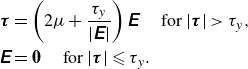 \begin{align}\boldsymbol{\tau} & =\left (2 \mu +\frac {\tau _y}{|\unicode{x1D640}|}\right) \unicode{x1D640}\quad \text{ for }|\boldsymbol{\tau }|\gt \tau _y, \nonumber\\ \unicode{x1D640} & =\boldsymbol{0}\quad \text{ for } |\boldsymbol{\tau }| \leqslant \tau _y. \end{align}
Here, $\tau _y$
is the yield stress,
$\tau _y$
is the yield stress, $\mu$
is the viscosity constant and
$\mu$
is the viscosity constant and $\unicode{x1D640}$
is the rate of strain tensor. The second invariant of a tensor is defined as
$\unicode{x1D640}$
is the rate of strain tensor. The second invariant of a tensor is defined as $|\boldsymbol{\delta }|= \sqrt {(\boldsymbol{\delta }: \boldsymbol{\delta })/2}$
for any tensor
$|\boldsymbol{\delta }|= \sqrt {(\boldsymbol{\delta }: \boldsymbol{\delta })/2}$
for any tensor $\boldsymbol{\delta } \in \mathbb{R}^{3 \times 3}$
. The Bingham model was employed to investigate the viscoplastic effect on the self-propulsion of a spherical squirmer (Eastham et al. Reference Eastham, Mohammadigoushki and Shoele2022), but it did not consider non-spherical body shapes.
$\boldsymbol{\delta } \in \mathbb{R}^{3 \times 3}$
. The Bingham model was employed to investigate the viscoplastic effect on the self-propulsion of a spherical squirmer (Eastham et al. Reference Eastham, Mohammadigoushki and Shoele2022), but it did not consider non-spherical body shapes.
We employ the augmented Lagrangian method proposed by Dean & Glowinski (Reference Dean and Glowinski2002) for the solution of the constitutive equation (2.12), which are rewritten as
 \begin{equation} \boldsymbol{\tau }=2 \mu \unicode{x1D640}+\tau _y \unicode{x1D63D}, \end{equation}
where $\unicode{x1D63D}$
is a non-dimensional tensor-valued function which satisfies
$\unicode{x1D63D}$
is a non-dimensional tensor-valued function which satisfies $|{\unicode{x1D63D}}| \leqslant 1$
,
$|{\unicode{x1D63D}}| \leqslant 1$
, ${\unicode{x1D63D}}:{\unicode{x1D640}} = |{\unicode{x1D640}}|$
, as well as the following relation (Dean & Glowinski Reference Dean and Glowinski2002)
${\unicode{x1D63D}}:{\unicode{x1D640}} = |{\unicode{x1D640}}|$
, as well as the following relation (Dean & Glowinski Reference Dean and Glowinski2002)
 \begin{equation} \unicode{x1D63D}=P_{\Lambda }\left (\unicode{x1D63D}+\sigma \tau _y \unicode{x1D640}\right) \quad \forall \ \sigma \gt 0, \end{equation}
where $P_{\Lambda }(\unicode{x1D666})$
is a symmetry-preserving orthogonal projection operator defined by
$P_{\Lambda }(\unicode{x1D666})$
is a symmetry-preserving orthogonal projection operator defined by
 \begin{equation} P_{\Lambda }(\unicode{x1D666})= \begin{cases}\unicode{x1D666} & \text{ if }|\unicode{x1D666}| \leqslant 1, \\ \unicode{x1D666}{/}|\unicode{x1D666}| & \text{ if }|\unicode{x1D666}|\gt 1.\end{cases} \end{equation}
Here, $\unicode{x1D666}$
represents a non-dimensional tensor. Equation (2.14) implies that
$\unicode{x1D666}$
represents a non-dimensional tensor. Equation (2.14) implies that $\unicode{x1D640} = \boldsymbol{0}$
when
$\unicode{x1D640} = \boldsymbol{0}$
when $| \unicode{x1D63D}+\sigma \tau _y \unicode{x1D640} | \leqslant 1$
and
$| \unicode{x1D63D}+\sigma \tau _y \unicode{x1D640} | \leqslant 1$
and $\unicode{x1D63D} = \unicode{x1D640}/|\unicode{x1D640}|$
when
$\unicode{x1D63D} = \unicode{x1D640}/|\unicode{x1D640}|$
when $| \unicode{x1D63D}+\sigma \tau _y \unicode{x1D640} | \gt 1$
, and thus (2.13) is equivalent to (2.12).
$| \unicode{x1D63D}+\sigma \tau _y \unicode{x1D640} | \gt 1$
, and thus (2.13) is equivalent to (2.12).
The following characteristic scales are used for the non-dimensionalisation scheme: $L_c = r_{eq}$
(
$L_c = r_{eq}$
( $r_{eq}= (b_xb_z^2)^{1/3}$
being the radius of a sphere with the same volume as the ellipsoid, i.e. the equivalent radius) for length,
$r_{eq}= (b_xb_z^2)^{1/3}$
being the radius of a sphere with the same volume as the ellipsoid, i.e. the equivalent radius) for length, $U_c = B_1$
for velocity,
$U_c = B_1$
for velocity, $t_c=L_{c}/U_c$
for time,
$t_c=L_{c}/U_c$
for time, $\mu U_c/L_c$
for stress and
$\mu U_c/L_c$
for stress and $\mu U_c/L^2_c$
for body force. For convenience, we write the dimensionless quantities in the same form as their dimensional counterparts, unless otherwise specified. By employing the variations
$\mu U_c/L^2_c$
for body force. For convenience, we write the dimensionless quantities in the same form as their dimensional counterparts, unless otherwise specified. By employing the variations $\boldsymbol{v}$
,
$\boldsymbol{v}$
, $\boldsymbol{V}$
and
$\boldsymbol{V}$
and $\boldsymbol{\xi }$
for the fluid velocity and the squirmer translational and angular velocities, respectively, the complete set of dimensionless governing equations in the weak form comprise the following three parts.
$\boldsymbol{\xi }$
for the fluid velocity and the squirmer translational and angular velocities, respectively, the complete set of dimensionless governing equations in the weak form comprise the following three parts.
(i) Equations of motion
 \begin{equation} Re \int _{\Omega }\left (\frac {\partial \boldsymbol{u}}{\partial t}+\boldsymbol{u} \cdot \nabla \boldsymbol{u}\right) \cdot \boldsymbol{v} \mathrm{d} \boldsymbol{x}=\int _{\Omega }(-\nabla p+ \nabla ^2 \boldsymbol{u}+Bi \nabla \cdot \unicode{x1D63D}) \cdot \boldsymbol{v}\,\mathrm{d} \boldsymbol{x}+\int _P \boldsymbol{\lambda } \cdot \boldsymbol{v}\ \mathrm{d} \boldsymbol{x}, \end{equation}
 \begin{equation} Re \left (\rho _r-1\right)\left (V_p\frac {\mathrm{d} \boldsymbol{U}}{\mathrm{d} t} \cdot \boldsymbol{V}+\unicode{x1D645} \cdot \frac {\mathrm{d} \boldsymbol{\omega }}{\mathrm{d} t} \cdot \boldsymbol{\xi }\right)=\int _P \!\!\left (Re {\frac {{\textrm {d}{\boldsymbol{u}_{a}}}}{{\textrm {d} t}}\textrm {d}{\boldsymbol{x}}}-\boldsymbol{\lambda }\right) \cdot (\boldsymbol{V}+\boldsymbol{\xi } \times \boldsymbol{r}) \mathrm{d} \boldsymbol{x}, \end{equation}
 \begin{equation} \int _P \left [\boldsymbol{u}-(\boldsymbol{U}+\boldsymbol{\omega } \times \boldsymbol{r})-\boldsymbol{u}_a \right] \cdot \boldsymbol{\gamma}\ \mathrm{d} \boldsymbol{x}=\mathbf{0}. \end{equation}
(ii) Continuity equation
 \begin{equation} \int _{\Omega } q \nabla \cdot \boldsymbol{u}\ \mathrm{d} \boldsymbol{x}=\mathbf{0}. \end{equation}
(iii) Constitutive equation
 \begin{equation} \unicode{x1D63D}=P_\Lambda \left (\unicode{x1D63D}+\sigma Bi \unicode{x1D640}\right) \quad \forall \ \sigma \gt 0. \end{equation}
In (2.18) and (2.19), $\boldsymbol{\gamma }$
and
$\boldsymbol{\gamma }$
and $q$
represent the corresponding variations. In this study,
$q$
represent the corresponding variations. In this study, $\rho _r=\rho _s/\rho _{\!f}$
is the swimmer–fluid density ratio, which is set to be unity. The following dimensionless numbers are introduced:
$\rho _r=\rho _s/\rho _{\!f}$
is the swimmer–fluid density ratio, which is set to be unity. The following dimensionless numbers are introduced:
 \begin{equation} {\textrm {Reynolds number}}:\ Re = \frac {{{\rho _{\!f}}{B_1}{r_{eq}}}}{{\mu }}, \end{equation}
 \begin{equation} {\textrm {Bingham number}}:\ Bi = \frac {{{\tau _y}{r_{eq}}}}{{\mu {B_1}}}. \end{equation}
The Bingham number here represents the non-dimensional yield stress.
2.3. Numerical method
Throughout this study, we set $\sigma =Re/(2Bi^2)$
in (2.20) as suggested by Dean & Glowinski (Reference Dean and Glowinski2002). The problem (2.16)–(2.20) is solved in an iterative way with the fractional step time scheme, as detailed in Yu & Wachs (Reference Yu and Wachs2007). The fictitious domain method for dealing with the swimming of a spherical or ellipsoidal squirmer in a Newtonian fluid has been validated in our previous studies (Lin & Gao Reference Lin and Gao2019; Xia et al. Reference Xia, Yu, Lin, Lin and Hu2025a
,Reference Xia, Yu, Zhang, Lin and Ouyang
b
). The accuracy for particle sedimentation in Bingham fluids was verified in Yu & Wachs (Reference Yu and Wachs2007). In this study, we validate the swimming speed, power dissipation and swimming efficiency in a Newtonian fluid against the theoretical results derived by Demir et al. (Reference Demir, van Gogh, Palaniappan and Nganguia2024). A convergence test is performed in Appendix B.
$\sigma =Re/(2Bi^2)$
in (2.20) as suggested by Dean & Glowinski (Reference Dean and Glowinski2002). The problem (2.16)–(2.20) is solved in an iterative way with the fractional step time scheme, as detailed in Yu & Wachs (Reference Yu and Wachs2007). The fictitious domain method for dealing with the swimming of a spherical or ellipsoidal squirmer in a Newtonian fluid has been validated in our previous studies (Lin & Gao Reference Lin and Gao2019; Xia et al. Reference Xia, Yu, Lin, Lin and Hu2025a
,Reference Xia, Yu, Zhang, Lin and Ouyang
b
). The accuracy for particle sedimentation in Bingham fluids was verified in Yu & Wachs (Reference Yu and Wachs2007). In this study, we validate the swimming speed, power dissipation and swimming efficiency in a Newtonian fluid against the theoretical results derived by Demir et al. (Reference Demir, van Gogh, Palaniappan and Nganguia2024). A convergence test is performed in Appendix B.
As shown in figure 1(a), a cubic periodic computational domain is adopted with $L_x=L_y=L_z=32r_{eq}$
. This configuration allows the squirmer to swim periodically through the domain. The computational domain is sufficiently large so that the effect of domain size completely disappears for a viscoplastic fluid, and it can reproduce an unbounded domain. According to the convergence test in Appendix B, 16 grid points are used across the squirmer’s equivalent radius (i.e.
$L_x=L_y=L_z=32r_{eq}$
. This configuration allows the squirmer to swim periodically through the domain. The computational domain is sufficiently large so that the effect of domain size completely disappears for a viscoplastic fluid, and it can reproduce an unbounded domain. According to the convergence test in Appendix B, 16 grid points are used across the squirmer’s equivalent radius (i.e. $r_{eq}/\Delta x=16$
) and the time step is set to be
$r_{eq}/\Delta x=16$
) and the time step is set to be $\Delta t = 10^{-4}r_{eq}/B_1$
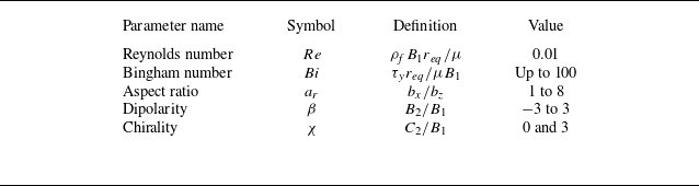
. The definitions and values of the non-dimensional parameters are summarised in table 1. In this paper, we consider a low Reynolds number of
$\Delta t = 10^{-4}r_{eq}/B_1$
. The definitions and values of the non-dimensional parameters are summarised in table 1. In this paper, we consider a low Reynolds number of $Re=0.01$
, which is small enough to neglect inertia. The aspect ratios range up to 8, corresponding to eccentricities up to 0.99. For each simulation, the squirmer was started from rest and allowed to accelerate until it reached a steady swimming speed. Simulation results were obtained after reaching a steady time-averaged swimming speed.
$Re=0.01$
, which is small enough to neglect inertia. The aspect ratios range up to 8, corresponding to eccentricities up to 0.99. For each simulation, the squirmer was started from rest and allowed to accelerate until it reached a steady swimming speed. Simulation results were obtained after reaching a steady time-averaged swimming speed.
Table 1. List of the non-dimensional simulation parameters.
3. Swimming in a viscoplastic fluid
In this section, we discuss the steady swimming speed $U$
, the power dissipation
$U$
, the power dissipation $P$
and the swimming efficiency
$P$
and the swimming efficiency $\eta$
for an ellipsoidal squirmer propelling in a viscoplastic fluid. The power
$\eta$
for an ellipsoidal squirmer propelling in a viscoplastic fluid. The power $P$
expended by the squirmer into the fluid is defined to be
$P$
expended by the squirmer into the fluid is defined to be
 \begin{equation} P=-\int _S(\boldsymbol{u} \cdot \boldsymbol{\tau }) \cdot \boldsymbol{n}\ \mathrm{d} s, \end{equation}
while the swimming efficiency is defined as the ratio of the power ( $P_D$
) required to tow a rigid ellipsoid in uniform motion at the swimming speed
$P_D$
) required to tow a rigid ellipsoid in uniform motion at the swimming speed $U$
of the squirmer to the work done by the squirmer
$U$
of the squirmer to the work done by the squirmer
 \begin{equation} \eta = \frac {{{P_D}}}{P} = \frac {{{\boldsymbol{F}_D} \cdot \boldsymbol{U}}}{P}, \end{equation}
where $\boldsymbol{F}_D$
is the force required to tow the passive particle with the same size and shape at the swimming speed
$\boldsymbol{F}_D$
is the force required to tow the passive particle with the same size and shape at the swimming speed $\boldsymbol{U}$
in the same fluid. The power dissipation
$\boldsymbol{U}$
in the same fluid. The power dissipation $P_N$
and swimming efficiency
$P_N$
and swimming efficiency $\eta _N$
for a non-swirling squirmer in a Newtonian fluid in the Stokes flow regime are derived theoretically by Demir et al. (Reference Demir, van Gogh, Palaniappan and Nganguia2024). In figures 3 and 9, we have compared the swimming speed, power dissipation, as well as swimming efficiency of a neutral swimmer and a puller with the theoretical solutions. The results demonstrate excellent agreement with the theory.
$\eta _N$
for a non-swirling squirmer in a Newtonian fluid in the Stokes flow regime are derived theoretically by Demir et al. (Reference Demir, van Gogh, Palaniappan and Nganguia2024). In figures 3 and 9, we have compared the swimming speed, power dissipation, as well as swimming efficiency of a neutral swimmer and a puller with the theoretical solutions. The results demonstrate excellent agreement with the theory.
3.1. Neutral squirmer
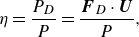
We compute the swimming speed, power dissipation and swimming efficiency relative to their corresponding Newtonian values as a function of Bingham number $Bi$
for both spherical and ellipsoidal neutral squirmers in figure 2. The results for the spherical squirmer (
$Bi$
for both spherical and ellipsoidal neutral squirmers in figure 2. The results for the spherical squirmer ( $a_r=1$
) agree well with results obtained from the finite element simulation of Eastham et al. (Reference Eastham, Mohammadigoushki and Shoele2022). From figure 2(a,b), we find that the squirmers for all aspect ratios swim slower and require more power than their Newtonian counterpart as the Bingham number increases. While the squirmer experiences a reduction in speed, more elongated squirmers are able to maintain speeds closer to that of their counterpart in Newtonian fluids. In the range of
$a_r=1$
) agree well with results obtained from the finite element simulation of Eastham et al. (Reference Eastham, Mohammadigoushki and Shoele2022). From figure 2(a,b), we find that the squirmers for all aspect ratios swim slower and require more power than their Newtonian counterpart as the Bingham number increases. While the squirmer experiences a reduction in speed, more elongated squirmers are able to maintain speeds closer to that of their counterpart in Newtonian fluids. In the range of $10 \leqslant Bi \leqslant 100$
, the power dissipation increases approximately exponentially with
$10 \leqslant Bi \leqslant 100$
, the power dissipation increases approximately exponentially with $Bi$
, following
$Bi$
, following $P/P_N \sim Bi^{0.83}$
from fitting, and is nearly independent of the aspect ratio. Although the power dissipation increases monotonically with the Bingham number, figure 2(c) shows that the variation in the swimming efficiency is non-monotonic as
$P/P_N \sim Bi^{0.83}$
from fitting, and is nearly independent of the aspect ratio. Although the power dissipation increases monotonically with the Bingham number, figure 2(c) shows that the variation in the swimming efficiency is non-monotonic as $Bi$
increases. The scaled swimming efficiency,
$Bi$
increases. The scaled swimming efficiency, $\eta /\eta _N$
, reaches a maximum value before decreasing to a low value. This behaviour has been reported by Eastham et al. (Reference Eastham, Mohammadigoushki and Shoele2022) for a spherical squirmer. The optimal Bingham number for maximum efficiency is smaller in the case of a long ellipsoid. At
$\eta /\eta _N$
, reaches a maximum value before decreasing to a low value. This behaviour has been reported by Eastham et al. (Reference Eastham, Mohammadigoushki and Shoele2022) for a spherical squirmer. The optimal Bingham number for maximum efficiency is smaller in the case of a long ellipsoid. At $Bi \leqslant 0.1$
, the elongated squirmer swims more efficiently, while the spherical squirmer has higher efficiency for moderate to high values of the Bingham number.
$Bi \leqslant 0.1$
, the elongated squirmer swims more efficiently, while the spherical squirmer has higher efficiency for moderate to high values of the Bingham number.
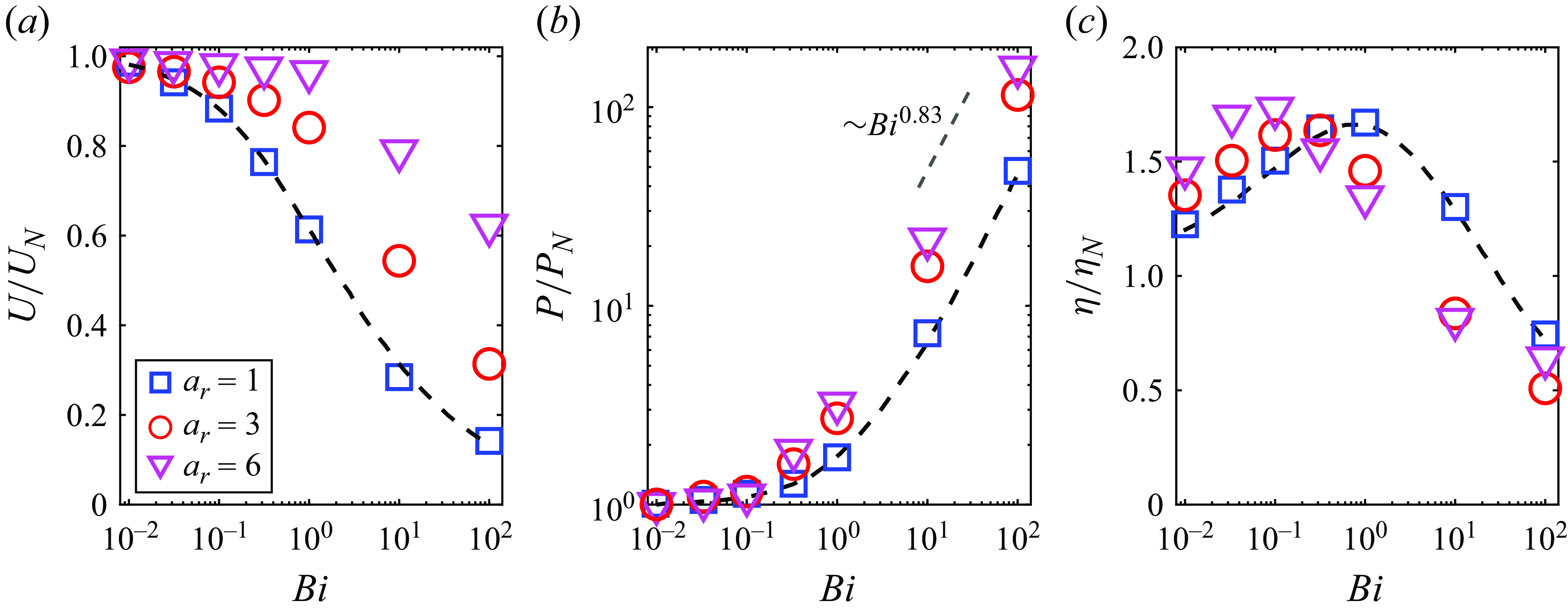
Figure 2. (a) Swimming speed $U$
, (b) power dissipation
$U$
, (b) power dissipation $P$
and (c) swimming efficiency
$P$
and (c) swimming efficiency $\eta$
, of a neutral squirmer, as a function of the Bingham number
$\eta$
, of a neutral squirmer, as a function of the Bingham number $Bi$
. The dashed lines represent the numerical results obtained using the continuous Galerkin finite element method for spherical squirmers, as presented in Eastham & Shoele (Reference Eastham and Shoele2020). Here, the results are scaled by the corresponding values for a squirmer in a Newtonian fluid.
$Bi$
. The dashed lines represent the numerical results obtained using the continuous Galerkin finite element method for spherical squirmers, as presented in Eastham & Shoele (Reference Eastham and Shoele2020). Here, the results are scaled by the corresponding values for a squirmer in a Newtonian fluid.
The observations in figure 2 can be made more clearly by plotting the results as a function of the aspect ratio for various $Bi$
. Figure 3(a) suggests that ellipsoidal squirmers swim much faster compared with spherical squirmers, and the influence of body shape on swimming speed becomes significantly more pronounced in environments with higher viscoplasticity. As illustrated in figure 3(b,c), ellipsoidal squirmers expend less energy and are more efficient swimmers compared with spherical squirmers for the same value of the Bingham number.
$Bi$
. Figure 3(a) suggests that ellipsoidal squirmers swim much faster compared with spherical squirmers, and the influence of body shape on swimming speed becomes significantly more pronounced in environments with higher viscoplasticity. As illustrated in figure 3(b,c), ellipsoidal squirmers expend less energy and are more efficient swimmers compared with spherical squirmers for the same value of the Bingham number.
Figure 3. (a) Normalised swimming speed, (b) normalised power dissipation and (c) swimming efficiency, of a neutral squirmer, as a function of aspect ratio. Curves are obtained from Demir et al. (Reference Demir, van Gogh, Palaniappan and Nganguia2024) for swimming in Newtonian fluids, while the symbols denote numerical results.
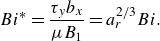
The results in figure 2 have been obtained for ellipsoidal microswimmers with constraints on volume, while some studies fixed the semi-major length $b_x$
when the aspect ratio changes (van Gogh et al. Reference van Gogh, Demir, Palaniappan and Pak2022; Demir et al. Reference Demir, van Gogh, Palaniappan and Nganguia2024). In figure 4, we replot figure 2 as a function of the modified Bingham number
$b_x$
when the aspect ratio changes (van Gogh et al. Reference van Gogh, Demir, Palaniappan and Pak2022; Demir et al. Reference Demir, van Gogh, Palaniappan and Nganguia2024). In figure 4, we replot figure 2 as a function of the modified Bingham number $Bi^*$
, which is defined as
$Bi^*$
, which is defined as
 \begin{equation} Bi^* = \frac {{{\tau _y}{b_x}}}{{\mu {B_1}}}=a^{2/3}_r Bi. \end{equation}
Our results show that the constraint of constant semi-major length does not qualitatively alter the results obtained under the fixed volume assumption. One interesting observation is that the scaled power dissipation has a much weaker dependence on the aspect ratio under the constant semi-major length constraint, as observed in figure 4(b). A similar weak dependence of particle shape on power dissipation has also been reported by Demir et al. (Reference Demir, van Gogh, Palaniappan and Nganguia2024) for a squirmer swimming through a heterogeneous medium with fixed semi-major axis length. Figure 4(c) exhibits a similar non-monotonic variation of the scaled efficiency with respect to $Bi$
, as observed in figure 2(c).
$Bi$
, as observed in figure 2(c).
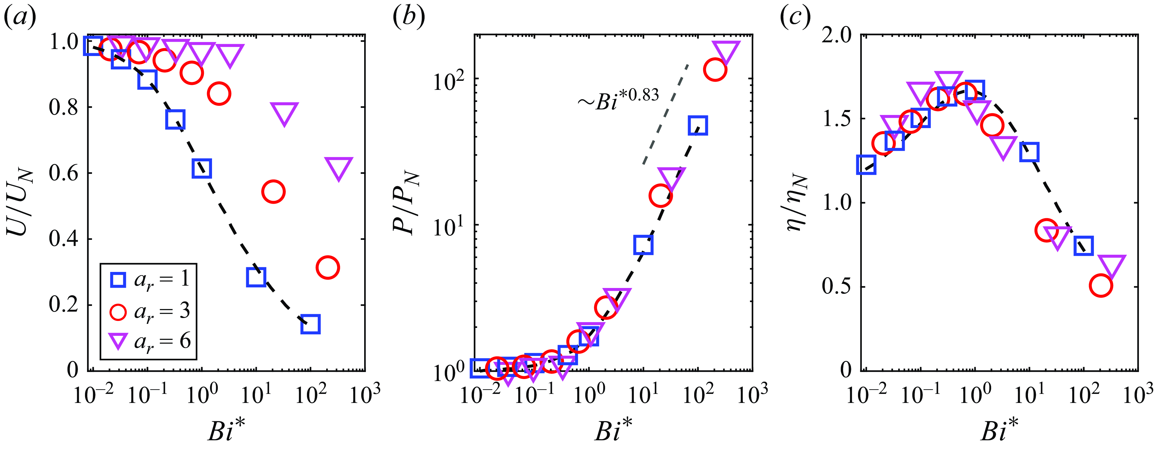
Figure 4. (a) Swimming speed $U$
, (b) power dissipation
$U$
, (b) power dissipation $P$
and (c) swimming efficiency
$P$
and (c) swimming efficiency $\eta$
, as a function of the modified Bingham number
$\eta$
, as a function of the modified Bingham number $Bi^*$
, defined by using the semi-major length
$Bi^*$
, defined by using the semi-major length $b_x$
. The results are normalised by their corresponding values for a neutral squirmer in a Newtonian fluid.
$b_x$
. The results are normalised by their corresponding values for a neutral squirmer in a Newtonian fluid.
The locomotion behaviour of spherical squirmer closely correlated with the confinement effects induced by the yielded region surrounding the swimming body (Eastham et al. Reference Eastham, Mohammadigoushki and Shoele2022). Figure 5(a–c) shows the yield-surface profiles around a neutral swimmer for various aspect ratios. The yield surface is given by the iso-surface of $\left |\boldsymbol{\tau }\right |=Bi$
. Indeed, increasing the Bingham number for a fixed aspect ratio results in a reduction of the yielded region around the squirmer and the plasticity becomes more dominant, as previously demonstrated by Eastham et al. (Reference Eastham, Mohammadigoushki and Shoele2022). The decreased swimming speed of neutral swimmers with increased confinement is also consistent with results from other models involving confinement (Reigh & Lauga Reference Reigh and Lauga2017; Nganguia et al. Reference Nganguia, Zhu, Palaniappan and Pak2020). By comparing figure 5(a–c), increasing the squirmer’s aspect ratio at a fixed Bingham number results in an expansion of the yielded region around the squirmer. Consequently, the ellipsoidal squirmer moves faster than the spherical squirmer for a given Bingham number. To gain further insight, we display in figure 5(d) the volume of the yielded region
$\left |\boldsymbol{\tau }\right |=Bi$
. Indeed, increasing the Bingham number for a fixed aspect ratio results in a reduction of the yielded region around the squirmer and the plasticity becomes more dominant, as previously demonstrated by Eastham et al. (Reference Eastham, Mohammadigoushki and Shoele2022). The decreased swimming speed of neutral swimmers with increased confinement is also consistent with results from other models involving confinement (Reigh & Lauga Reference Reigh and Lauga2017; Nganguia et al. Reference Nganguia, Zhu, Palaniappan and Pak2020). By comparing figure 5(a–c), increasing the squirmer’s aspect ratio at a fixed Bingham number results in an expansion of the yielded region around the squirmer. Consequently, the ellipsoidal squirmer moves faster than the spherical squirmer for a given Bingham number. To gain further insight, we display in figure 5(d) the volume of the yielded region $V_Y$
normalised by the squirmer volume
$V_Y$
normalised by the squirmer volume $V_p$
versus the Bingham number. It can be observed that the volume of the yielded region
$V_p$
versus the Bingham number. It can be observed that the volume of the yielded region $V_Y$
decreases with
$V_Y$
decreases with $Bi$
and increases as the squirmer’s aspect ratio becomes larger. At low yield stress, the volume of the yielded regime declines as
$Bi$
and increases as the squirmer’s aspect ratio becomes larger. At low yield stress, the volume of the yielded regime declines as $V_Y \sim Bi^{-3/4}$
for all aspect ratios. This scaling can be derived by assuming
$V_Y \sim Bi^{-3/4}$
for all aspect ratios. This scaling can be derived by assuming ${V_Y} \sim {r^3_Y}$
, with
${V_Y} \sim {r^3_Y}$
, with $r_Y$
being the radius of the yielded regime (i.e.
$r_Y$
being the radius of the yielded regime (i.e. ${\left | \boldsymbol{\tau } \right |_{r = {r_Y}}} = Bi$
). As will be discussed in the next paragraph, the velocity disturbance induced by a neutral squirmer in the far field decays as
${\left | \boldsymbol{\tau } \right |_{r = {r_Y}}} = Bi$
). As will be discussed in the next paragraph, the velocity disturbance induced by a neutral squirmer in the far field decays as $r^{-3}$
in the limit
$r^{-3}$
in the limit $Bi \to 0$
, where
$Bi \to 0$
, where $r$
is the distance. The derivative of the velocity disturbance decays as
$r$
is the distance. The derivative of the velocity disturbance decays as $r^{-4}$
, so
$r^{-4}$
, so $\left | \boldsymbol{\tau } \right |$
also decays as
$\left | \boldsymbol{\tau } \right |$
also decays as $\left | \boldsymbol{\tau } \right | \sim {r^{ - 4}}$
, leading to
$\left | \boldsymbol{\tau } \right | \sim {r^{ - 4}}$
, leading to $r_Y^{ - 4} \sim Bi$
. As a result, we obtain the scaling of
$r_Y^{ - 4} \sim Bi$
. As a result, we obtain the scaling of ${V_Y} \sim B{i^{ - 3/4}}$
. However, as the Bingham number increases, the yield surface progressively shrinks toward the squirmer’s surface, and the adopted scaling assuming the far-field decay tendency fails to hold for
${V_Y} \sim B{i^{ - 3/4}}$
. However, as the Bingham number increases, the yield surface progressively shrinks toward the squirmer’s surface, and the adopted scaling assuming the far-field decay tendency fails to hold for $Bi \gg O(10^{-1})$
. Specifically, the more elongated squirmer has a greater impact on the shape of the yield surface, producing a much larger yielded region. Thus, in high
$Bi \gg O(10^{-1})$
. Specifically, the more elongated squirmer has a greater impact on the shape of the yield surface, producing a much larger yielded region. Thus, in high $Bi$
environments, the yielded region around an ellipsoidal squirmer is significantly larger than that around a spherical squirmer, resulting in a much higher swimming speed for the ellipsoidal squirmer compared with the spherical one.
$Bi$
environments, the yielded region around an ellipsoidal squirmer is significantly larger than that around a spherical squirmer, resulting in a much higher swimming speed for the ellipsoidal squirmer compared with the spherical one.
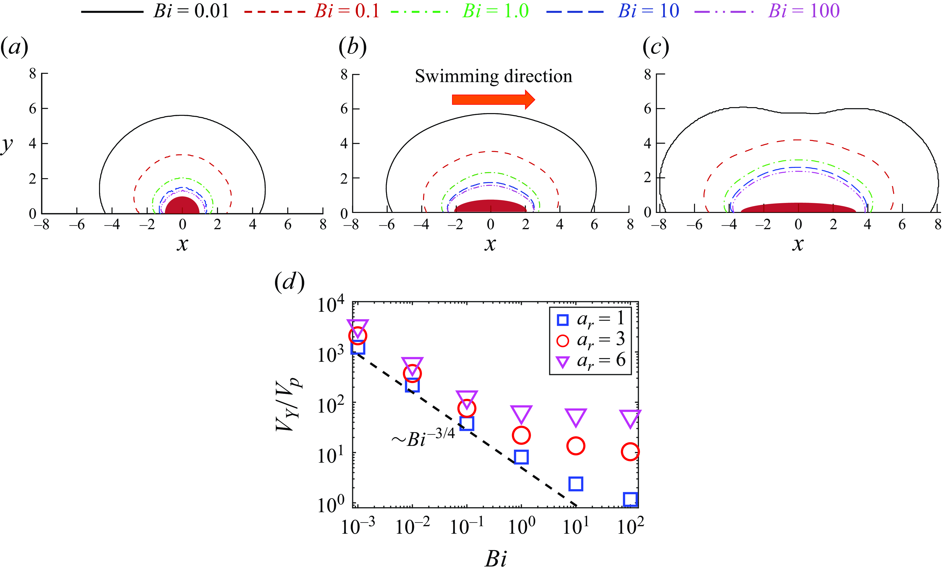
Figure 5. Yield-surface profiles around a neutral swimmer ( $\beta =0$
) for various
$\beta =0$
) for various $Bi$
. Panels show (a)
$Bi$
. Panels show (a) $a_r=1$
, (b)
$a_r=1$
, (b) $a_r=3$
, (c)
$a_r=3$
, (c) $a_r=6$
. (d) Volume of the yielded region as a function of
$a_r=6$
. (d) Volume of the yielded region as a function of $Bi$
. The dashed line in (d) is added to represent the slope
$Bi$
. The dashed line in (d) is added to represent the slope $Bi^{-3/4}$
. The yield surface is given by the iso-surface of
$Bi^{-3/4}$
. The yield surface is given by the iso-surface of $|\boldsymbol{\tau }|=Bi$
.
$|\boldsymbol{\tau }|=Bi$
.
The flow decay around a microswimmer is important for discussing the interaction of microswimmers and tracer diffusion. Since the stresslet of a neutral squirmer is zero, the flow decays as $\sim{\kern-1pt}r^{-3}$
in a Newtonian fluid in the far field (Theers et al. Reference Theers, Westphal, Gompper and Winkler2016). figure 6(a,b) shows the component of fluid velocity
$\sim{\kern-1pt}r^{-3}$
in a Newtonian fluid in the far field (Theers et al. Reference Theers, Westphal, Gompper and Winkler2016). figure 6(a,b) shows the component of fluid velocity $u$
in the swimming direction versus the position relative to the squirmer centre along the semi-major axis for different aspect ratio for fixed Bingham numbers of
$u$
in the swimming direction versus the position relative to the squirmer centre along the semi-major axis for different aspect ratio for fixed Bingham numbers of $Bi=0.01$
and 1.0, respectively. The decay tendency of
$Bi=0.01$
and 1.0, respectively. The decay tendency of $r^{-3}$
is marginally observed for a spherical squirmer with
$r^{-3}$
is marginally observed for a spherical squirmer with $Bi = 0.01$
. The flow decreases significantly with increasing distance, rapidly becoming negligible in the vicinity of the yield surface. For a mild viscoplastic environment of
$Bi = 0.01$
. The flow decreases significantly with increasing distance, rapidly becoming negligible in the vicinity of the yield surface. For a mild viscoplastic environment of $Bi=1.0$
, the velocity reduces to a negligible value (i.e.
$Bi=1.0$
, the velocity reduces to a negligible value (i.e. $u/U \lt 10^{-4}$
) at
$u/U \lt 10^{-4}$
) at $x/b_x \lt 1.6$
, implying that near-field fluid mechanics dominates. When we fix
$x/b_x \lt 1.6$
, implying that near-field fluid mechanics dominates. When we fix $a_r=3$
instead, and vary the Bingham number (figure 6
c), we observe that the flow decreases significantly with increasing Bingham number. This trend is consistent with the results in figure 2(a) and figure 4(a) that show that the propulsion speed decreases monotonically with increasing Bingham number. The results in figure 6 differ from the observed behaviour in Newtonian fluids and heterogeneous media (Demir et al. Reference Demir, van Gogh, Palaniappan and Nganguia2024). In viscoplastic fluids, the flow decays much faster than in Newtonian fluids and heterogeneous media, where the flow decays as
$a_r=3$
instead, and vary the Bingham number (figure 6
c), we observe that the flow decreases significantly with increasing Bingham number. This trend is consistent with the results in figure 2(a) and figure 4(a) that show that the propulsion speed decreases monotonically with increasing Bingham number. The results in figure 6 differ from the observed behaviour in Newtonian fluids and heterogeneous media (Demir et al. Reference Demir, van Gogh, Palaniappan and Nganguia2024). In viscoplastic fluids, the flow decays much faster than in Newtonian fluids and heterogeneous media, where the flow decays as $\sim{\kern-1pt}r^{-3}$
in the far field, regardless of the shape of the microswimmer.
$\sim{\kern-1pt}r^{-3}$
in the far field, regardless of the shape of the microswimmer.
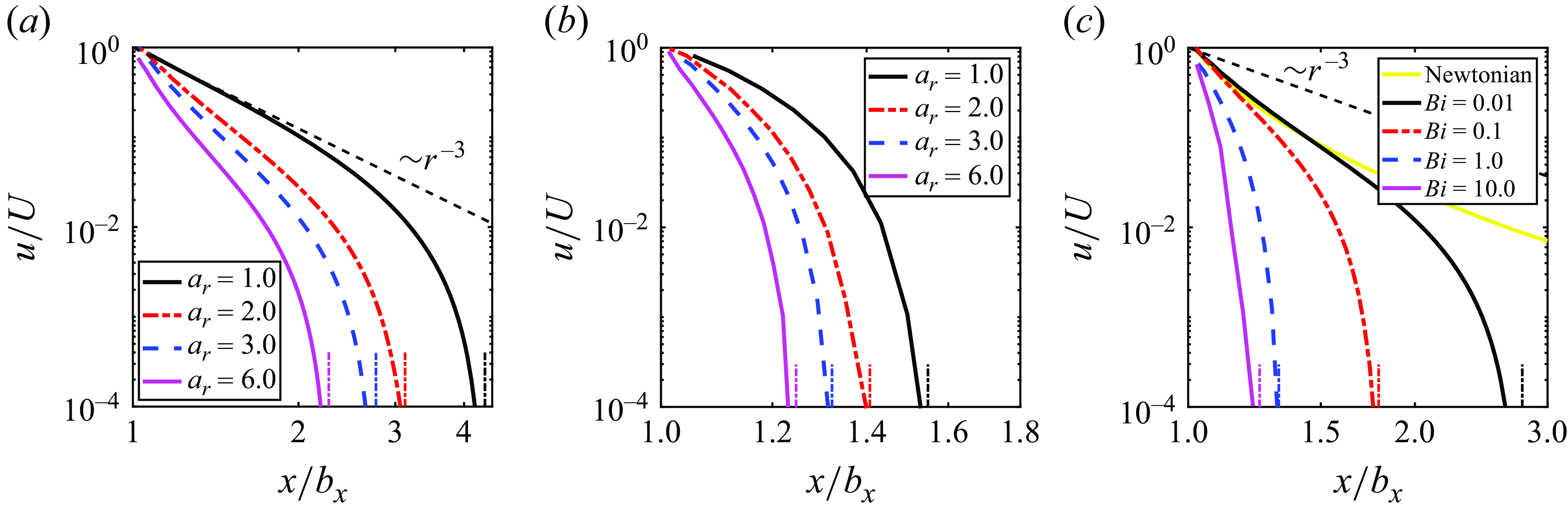
Figure 6. Laboratory-frame velocity component in the swimming direction scaled by the swimming speed $U$
versus the position relative to the centre of squirmer along the semi-major axis. (a,b) Effect of aspect ratio for (a)
$U$
versus the position relative to the centre of squirmer along the semi-major axis. (a,b) Effect of aspect ratio for (a) $Bi=0.01$
and (b)
$Bi=0.01$
and (b) $Bi=1.0$
. (c) Effect of the Bingham number on velocity for
$Bi=1.0$
. (c) Effect of the Bingham number on velocity for $a_r=3$
. Here,
$a_r=3$
. Here, $x/b_x=1$
corresponds to the particle’s surface. The black dash line is added to represent the slope
$x/b_x=1$
corresponds to the particle’s surface. The black dash line is added to represent the slope $\sim{\kern-1pt}r^{-3}$
. The vertical dash-dot lines indicate the corresponding positions of the yield surface, where the flow properties undergo rapid transition.
$\sim{\kern-1pt}r^{-3}$
. The vertical dash-dot lines indicate the corresponding positions of the yield surface, where the flow properties undergo rapid transition.
To better understand the flow convergence near the yield surface, we further examine the fluid velocity profiles in this region. As described figure 7, the flow increases from the yield surface following $r^3$
apart from the vicinity of the squirmer, where
$r^3$
apart from the vicinity of the squirmer, where $r$
is the distance from the wall. This scaling is regardless of either the Bingham number or squirmer’s aspect ratio, offering a consistent description of the near-yield-surface flow behaviour. From figure 7(b,c), the fluid velocity can be reasonably approximated as
$r$
is the distance from the wall. This scaling is regardless of either the Bingham number or squirmer’s aspect ratio, offering a consistent description of the near-yield-surface flow behaviour. From figure 7(b,c), the fluid velocity can be reasonably approximated as $u=A(x_Y-x)^3$
in the whole yielded region for
$u=A(x_Y-x)^3$
in the whole yielded region for $Bi \geqslant 1$
. Here
$Bi \geqslant 1$
. Here $A$
is a coefficient related to the squirmer’s aspect ratio and Bingham number. To understand the
$A$
is a coefficient related to the squirmer’s aspect ratio and Bingham number. To understand the $r^3$
growth, consider how the velocity disturbance induced by a point force in a Newtonian fluid grows in the vicinity of an infinite flat plate. The Blakelet solution (Blake Reference Blake1975) provides
$r^3$
growth, consider how the velocity disturbance induced by a point force in a Newtonian fluid grows in the vicinity of an infinite flat plate. The Blakelet solution (Blake Reference Blake1975) provides $r^2$
growth of the velocity disturbance in a Newtonian fluid near a flat plate, in the direction perpendicular to the wall, which is slower than in the Bingham fluid. Since the apparent viscosity of the Bingham fluid increases as the velocity gradient decreases, the viscosity increases near the wall and the velocity decays rapidly. This can be one reason for the faster growth of the velocity in the Bingham fluid. While universal theory is not currently available, it will be an important focus of our future work.
$r^2$
growth of the velocity disturbance in a Newtonian fluid near a flat plate, in the direction perpendicular to the wall, which is slower than in the Bingham fluid. Since the apparent viscosity of the Bingham fluid increases as the velocity gradient decreases, the viscosity increases near the wall and the velocity decays rapidly. This can be one reason for the faster growth of the velocity in the Bingham fluid. While universal theory is not currently available, it will be an important focus of our future work.
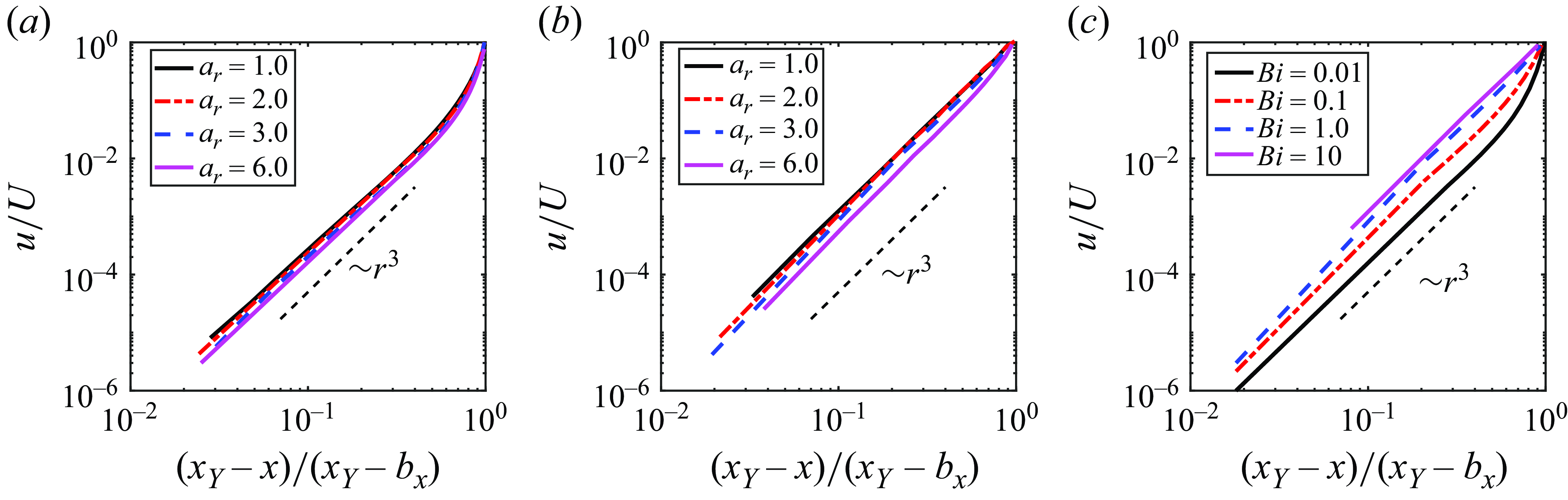
Figure 7. Laboratory-frame velocity component in the swimming direction scaled by the swimming speed $U$
versus the position relative to the position of the yield surface along the semi-major axis. (a,b) Effect of aspect ratio for (a)
$U$
versus the position relative to the position of the yield surface along the semi-major axis. (a,b) Effect of aspect ratio for (a) $Bi=0.01$
and (b)
$Bi=0.01$
and (b) $Bi=1.0$
. (c) Effect of the Bingham number on velocity for
$Bi=1.0$
. (c) Effect of the Bingham number on velocity for $a_r=3$
. Here,
$a_r=3$
. Here, $x_Y$
represents the relative coordinate of the yield surface in the x-direction, thus
$x_Y$
represents the relative coordinate of the yield surface in the x-direction, thus $(x_Y -x)/(x_Y-b_x) = 0$
corresponds to the position of the yield surface. The black dash line is added to represent the slope
$(x_Y -x)/(x_Y-b_x) = 0$
corresponds to the position of the yield surface. The black dash line is added to represent the slope $\sim{\kern-1pt}r^{3}$
.
$\sim{\kern-1pt}r^{3}$
.
3.2. Pullers and pushers
In Stokes flow of a Newtonian fluid, the swimming speed of a squirmer is independent of the swimming dipolarity $\beta$
. In contrast, in a viscoelastic fluid, the swimming speed depends on the value of
$\beta$
. In contrast, in a viscoelastic fluid, the swimming speed depends on the value of $\beta$
. For a spherical squirmer in an upper convected Maxwell fluid, the speed is given by
$\beta$
. For a spherical squirmer in an upper convected Maxwell fluid, the speed is given by $U/U_N=1-0.2\beta Wi$
, where
$U/U_N=1-0.2\beta Wi$
, where $Wi$
is the Weissenberg number (Datt & Elfring Reference Datt and Elfring2019). This equation indicates that the swimming speed decreases for positive values of
$Wi$
is the Weissenberg number (Datt & Elfring Reference Datt and Elfring2019). This equation indicates that the swimming speed decreases for positive values of $\beta$
and increases for negative values. It is reasonable to discuss the swimmer type dependence on the locomotion of the squirmer in a viscoplastic fluid. To address this question, we study cases of a puller/pusher (
$\beta$
and increases for negative values. It is reasonable to discuss the swimmer type dependence on the locomotion of the squirmer in a viscoplastic fluid. To address this question, we study cases of a puller/pusher ( $\left | \beta \right |=3$
) with higher polar modes
$\left | \beta \right |=3$
) with higher polar modes $B_{n\gt 2}$
and
$B_{n\gt 2}$
and $C_n$
set to zero. We examine the velocity fields around the pushers, pullers and neutral swimmers in a Bingham environment in figure 8, where the yield surface is shown with the dash lines. By comparing figure 8(a,b,c) or (d,e, f), one can observe that the flow field and the yield surface are symmetrical for
$C_n$
set to zero. We examine the velocity fields around the pushers, pullers and neutral swimmers in a Bingham environment in figure 8, where the yield surface is shown with the dash lines. By comparing figure 8(a,b,c) or (d,e, f), one can observe that the flow field and the yield surface are symmetrical for $\beta =3$
and −3, but different for neutral swimmers. We compare the swimming speed, power dissipation and efficiency among pullers, pushers and neutral swimmers in table 2. We find that these values differ between neutral swimmers and pullers or pushers, but are independent of the sign of
$\beta =3$
and −3, but different for neutral swimmers. We compare the swimming speed, power dissipation and efficiency among pullers, pushers and neutral swimmers in table 2. We find that these values differ between neutral swimmers and pullers or pushers, but are independent of the sign of $\beta$
(i.e. puller versus pusher). In some cases, the puller/pusher may swim faster than the neutral swimmer, but in others, it may swim slower. However, its swimming efficiency is much lower than that of a neutral swimmer, as the second polar mode contributes to mixing of the surrounding fluid and increases power dissipation.
$\beta$
(i.e. puller versus pusher). In some cases, the puller/pusher may swim faster than the neutral swimmer, but in others, it may swim slower. However, its swimming efficiency is much lower than that of a neutral swimmer, as the second polar mode contributes to mixing of the surrounding fluid and increases power dissipation.
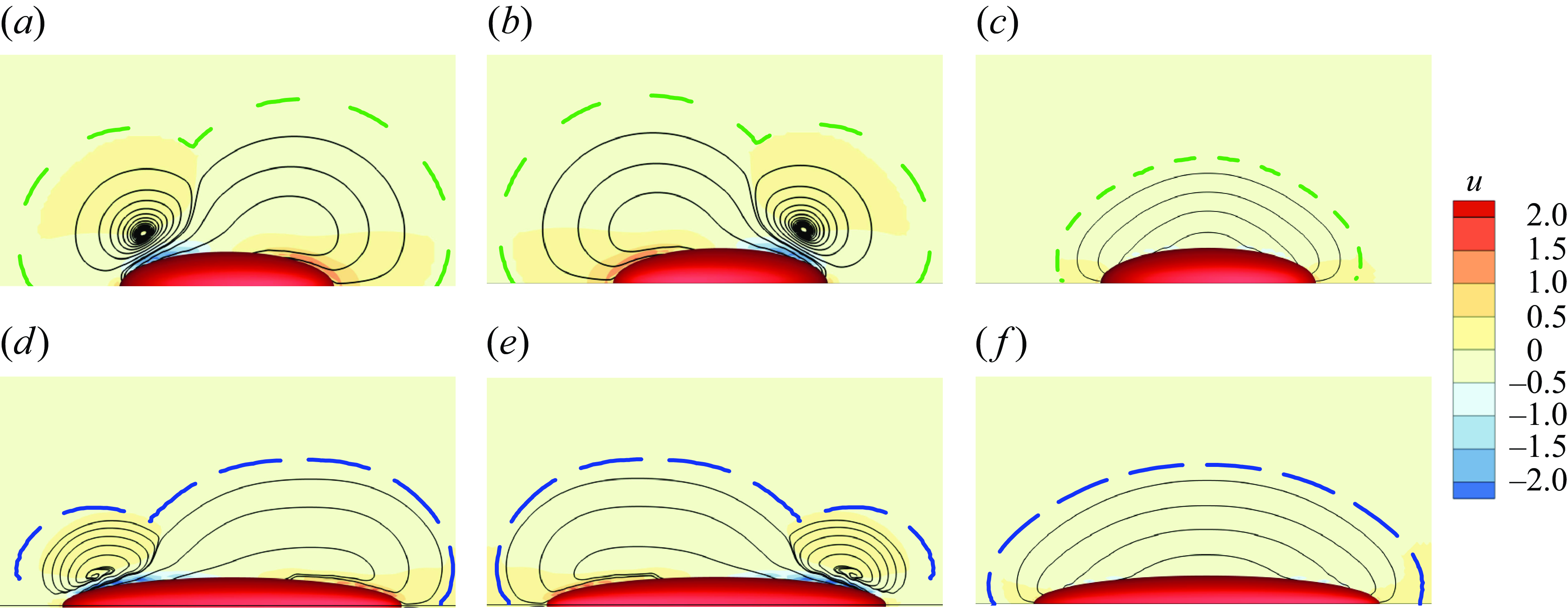
Figure 8. The velocity fields (colours) and streamlines (black lines) for (a,b,c) $Bi=1$
and
$Bi=1$
and $a_r=3$
, (d,e, f)
$a_r=3$
, (d,e, f) $Bi=10$
and
$Bi=10$
and $a_r=6$
. Panels show (a,d)
$a_r=6$
. Panels show (a,d) $\beta =-3$
, (b,e)
$\beta =-3$
, (b,e) $\beta =3$
and (c, f)
$\beta =3$
and (c, f) $\beta =0$
. The green or blue lines represent the yield surface, while the black lines are the streamlines.
$\beta =0$
. The green or blue lines represent the yield surface, while the black lines are the streamlines.
Table 2. List of the normalised swimming speed, power dissipation and swimming efficiency for specific cases of a pusher, puller and neutral swimmer in a viscoplastic fluid.

Figure 9 shows the normalised propulsion speed, power dissipation and swimming efficiency of a puller ( $\beta =3$
) as a function of aspect ratio. The results show that the puller uses more energy and swims more slowly in viscoplastic fluids. In addition, ellipsoidal pullers swim faster with increasing aspect ratio for a given Bingham number. By comparing figures 9(b) and 3(b), we observe that ellipsoidal pullers expend more energy compared with spherical pullers, while ellipsoidal neutral swimmers expend less energy compared with spherical swimmers. As illustrated in figure 9(c), the hydrodynamic efficiency in viscoplastic fluids is non-monotonic: it first decreases as
$\beta =3$
) as a function of aspect ratio. The results show that the puller uses more energy and swims more slowly in viscoplastic fluids. In addition, ellipsoidal pullers swim faster with increasing aspect ratio for a given Bingham number. By comparing figures 9(b) and 3(b), we observe that ellipsoidal pullers expend more energy compared with spherical pullers, while ellipsoidal neutral swimmers expend less energy compared with spherical swimmers. As illustrated in figure 9(c), the hydrodynamic efficiency in viscoplastic fluids is non-monotonic: it first decreases as $a_r$
approaches 1.5–2, and then increases for
$a_r$
approaches 1.5–2, and then increases for $a_r\gt 2$
.
$a_r\gt 2$
.
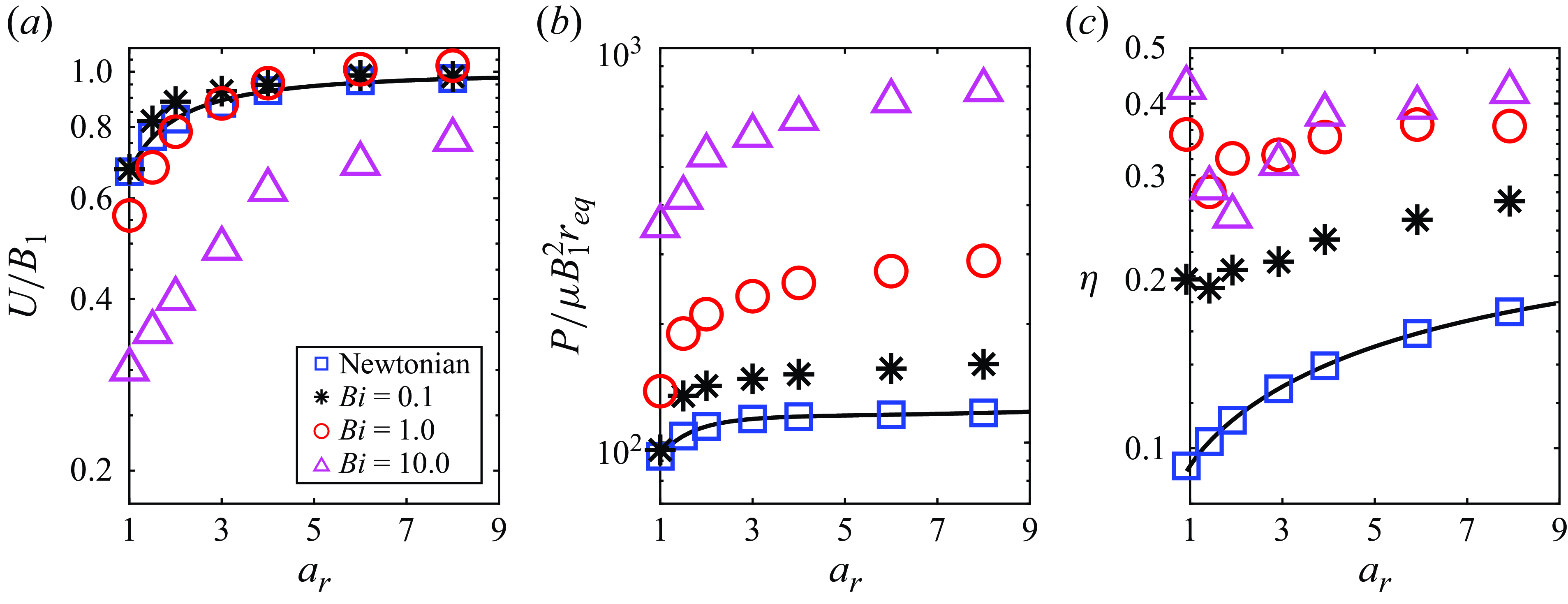
Figure 9. (a) Normalised swimming speed, (b) normalised power dissipation and (c) swimming efficiency, of a puller ( $\beta =3$
), as a function of aspect ratio. Curves are obtained from Demir et al. (Reference Demir, van Gogh, Palaniappan and Nganguia2024) for swimming in Newtonian fluids, while the symbols denote numerical results.
$\beta =3$
), as a function of aspect ratio. Curves are obtained from Demir et al. (Reference Demir, van Gogh, Palaniappan and Nganguia2024) for swimming in Newtonian fluids, while the symbols denote numerical results.
In order to highlight the dependence of the squirmer’s aspect ratio and Bingham number on the swimming speed variation due to the second polar mode, we plot a phase map in figure 10(a), which shows the regimes where speed-enhanced ( $U_{\beta =3}/U_{\beta =0} \gt 1$
) and hindered (
$U_{\beta =3}/U_{\beta =0} \gt 1$
) and hindered ( $U_{\beta =3}/U_{\beta =0} \lt 1$
) swimming occur in the
$U_{\beta =3}/U_{\beta =0} \lt 1$
) swimming occur in the $a_r$
–
$a_r$
– $Bi$
space. By applying data fitting, the transition condition for
$Bi$
space. By applying data fitting, the transition condition for $U_{\beta =3}/U_{\beta =0}=1$
is represented by a dashed curve in the figure. It is observed that the second polar mode only reduces the swimming speed of elongated squirmers in a strongly viscoplastic environment when
$U_{\beta =3}/U_{\beta =0}=1$
is represented by a dashed curve in the figure. It is observed that the second polar mode only reduces the swimming speed of elongated squirmers in a strongly viscoplastic environment when $a_r$
exceeds a critical value, while in other scenarios, it enhances the speed. The ratio
$a_r$
exceeds a critical value, while in other scenarios, it enhances the speed. The ratio $U_{\beta =3}/U_{\beta =0}$
as a function of the aspect ratio
$U_{\beta =3}/U_{\beta =0}$
as a function of the aspect ratio $a_r$
is shown in figure 10(b). As a general trend,
$a_r$
is shown in figure 10(b). As a general trend, $U_{\beta =3}/U_{\beta =0}$
decreases with increasing
$U_{\beta =3}/U_{\beta =0}$
decreases with increasing $a_r$
for a fixed value of Bingham number. Specifically, the speed of a spherical puller is approximately 1.7 times greater than that of a spherical neutral swimmer at
$a_r$
for a fixed value of Bingham number. Specifically, the speed of a spherical puller is approximately 1.7 times greater than that of a spherical neutral swimmer at $Bi=100$
, whereas the speed of an elongated puller (
$Bi=100$
, whereas the speed of an elongated puller ( $a_r \gt 4$
) is only half that of the neutral squirmer. To understand this behaviour, we compare the volume of the yielded regime for pullers and neutral swimmers in figure 10(c) as a function of
$a_r \gt 4$
) is only half that of the neutral squirmer. To understand this behaviour, we compare the volume of the yielded regime for pullers and neutral swimmers in figure 10(c) as a function of $Bi$
. The results indicate that the volume of the yielded region depends on both the Bingham number and the body shape. In general, the second polar mode consistently increases the volume of the yielded region for a spherical squirmer, leading to a speedup of the squirmer. However, for ellipsoidal squirmers with aspect ratios exceeding a certain value, the yielded region created by the polar mode is much smaller than that of neutral squirmers at large Bingham numbers (
$Bi$
. The results indicate that the volume of the yielded region depends on both the Bingham number and the body shape. In general, the second polar mode consistently increases the volume of the yielded region for a spherical squirmer, leading to a speedup of the squirmer. However, for ellipsoidal squirmers with aspect ratios exceeding a certain value, the yielded region created by the polar mode is much smaller than that of neutral squirmers at large Bingham numbers ( $Bi \geqslant 10$
). As a result, the increased confinement slows down the ellipsoidal squirmer.
$Bi \geqslant 10$
). As a result, the increased confinement slows down the ellipsoidal squirmer.
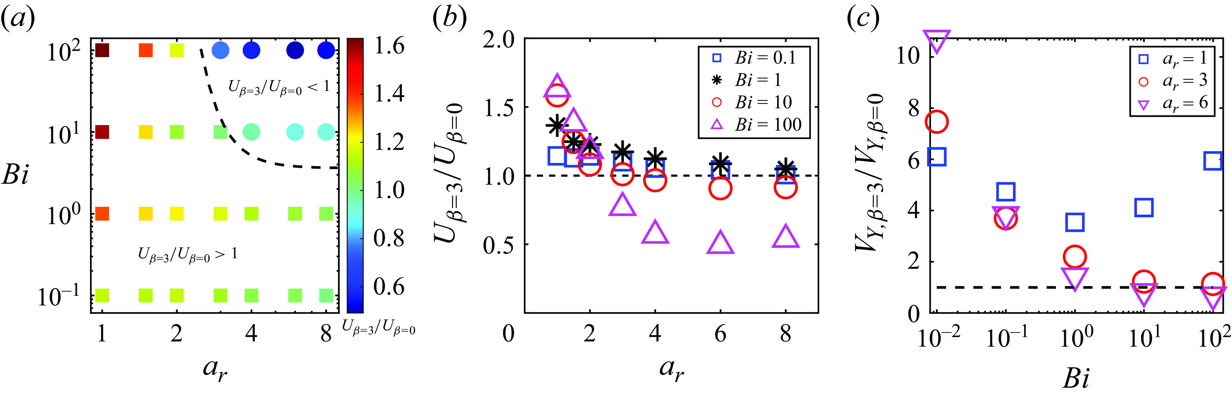
Figure 10. Ratio of swimming speed between a puller ( $\beta =3$
) and a neutral squirmer in a viscoplastic fluid. (a) Phase diagram over the aspect ratio
$\beta =3$
) and a neutral squirmer in a viscoplastic fluid. (a) Phase diagram over the aspect ratio $a_r$
and Bingham number
$a_r$
and Bingham number $Bi$
. Symbols are coloured by the speed ratio
$Bi$
. Symbols are coloured by the speed ratio $U_{\beta =3}/U_{\beta =0}$
, and the dashed line gives the boundary between these states by data fitting. (b) Value of
$U_{\beta =3}/U_{\beta =0}$
, and the dashed line gives the boundary between these states by data fitting. (b) Value of $U_{\beta =3}/U_{\beta =0}$
as a function of the Bingham number
$U_{\beta =3}/U_{\beta =0}$
as a function of the Bingham number $Bi$
as a function of the aspect ratio. (c) Normalised volume of yielded region
$Bi$
as a function of the aspect ratio. (c) Normalised volume of yielded region $V_{Y,\beta =3}/V_{Y,\beta =0}$
as a function of
$V_{Y,\beta =3}/V_{Y,\beta =0}$
as a function of $Bi$
.
$Bi$
.
3.3. Neutral swirling squirmer
The swirling mode plays a role in complex fluids such as viscoelastic fluids. Theoretical and numerical studies have indicated that the swimming speed of squirmers is enhanced due to the coupling between chirality and viscoelasticity (Binagia et al. Reference Binagia, Phoa, Housiadas and Shaqfeh2020; Housiadas et al. Reference Housiadas, Binagia and Shaqfeh2021). In particular, previous studies highlight the critical role of the first normal stress difference induced by the swirling flow in boosting swimming speeds (Binagia & Shaqfeh Reference Binagia and Shaqfeh2021; Kobayashi et al. Reference Kobayashi, Molina and Yamamoto2024). To date, however, no one has considered how the presence of the azimuthal modes in the squirmer model impacts the swimming kinematics in a viscoplastic fluid, and studies of swirling squirmers in complex fluids have been limited to spherical shapes.
In the $a_r$
–
$a_r$
– $Bi$
plane plotted in figure 11(a), we report the change in swimming speed when introducing the second swirling mode (
$Bi$
plane plotted in figure 11(a), we report the change in swimming speed when introducing the second swirling mode ( $\chi =3$
) relative to its non-swirling counterpart (i.e.
$\chi =3$
) relative to its non-swirling counterpart (i.e. $U_{\chi =3}/U_{\chi =0}$
) for different parameter points. Similar to our observation in figure 10(a), while the swirling motion generally contributes to an increase in the swimming speed of a squirmer for small
$U_{\chi =3}/U_{\chi =0}$
) for different parameter points. Similar to our observation in figure 10(a), while the swirling motion generally contributes to an increase in the swimming speed of a squirmer for small $a_r$
, beyond a given threshold in aspect ratio and/or Bingham number, the swirling squirmer swims slower than the non-swirling swimmer with the same
$a_r$
, beyond a given threshold in aspect ratio and/or Bingham number, the swirling squirmer swims slower than the non-swirling swimmer with the same $a_r$
and
$a_r$
and $Bi$
. The transition condition for
$Bi$
. The transition condition for $U_{\chi =3}/U_{\chi =0}=1$
is fitted and represented by a dashed curve in the figure. In figure 11(b), we show that
$U_{\chi =3}/U_{\chi =0}=1$
is fitted and represented by a dashed curve in the figure. In figure 11(b), we show that $U_{\chi =3}/U_{\chi =0}$
decreases with the aspect ratio, similar to the results observed in figure 10(b). Specifically, the speed enhancement of a spherical swirling squirmer relative to a non-swirling squirmer is approximately 1.7 times at
$U_{\chi =3}/U_{\chi =0}$
decreases with the aspect ratio, similar to the results observed in figure 10(b). Specifically, the speed enhancement of a spherical swirling squirmer relative to a non-swirling squirmer is approximately 1.7 times at $Bi=100$
, while the speed of ellipsoidal squirmers with large aspect ratios is significantly reduced by the swirling mode. We plot the variation in the normalised volume of the yielded region (
$Bi=100$
, while the speed of ellipsoidal squirmers with large aspect ratios is significantly reduced by the swirling mode. We plot the variation in the normalised volume of the yielded region ( $V_{Y,\chi =3}/V_{Y,\chi =0}$
) in figure 11(c). For all aspect ratios,
$V_{Y,\chi =3}/V_{Y,\chi =0}$
) in figure 11(c). For all aspect ratios, $V_{Y,\chi =3}/V_{Y,\chi =0}$
first increases with increasing
$V_{Y,\chi =3}/V_{Y,\chi =0}$
first increases with increasing $Bi$
, reaching a local maximum at
$Bi$
, reaching a local maximum at $Bi=O(10^{-1})$
, then becomes smaller as
$Bi=O(10^{-1})$
, then becomes smaller as $Bi$
continues to increase. For a spherical squirmer, the swirling mode always increases the volume of the yielded region. However, for ellipsoidal squirmers, the yielded region generated by swirling squirmers can be much smaller than that of non-swirling squirmers at large Bingham numbers. As a result, the increased confinement reduces the speed of the squirmer with a large aspect ratio.
$Bi$
continues to increase. For a spherical squirmer, the swirling mode always increases the volume of the yielded region. However, for ellipsoidal squirmers, the yielded region generated by swirling squirmers can be much smaller than that of non-swirling squirmers at large Bingham numbers. As a result, the increased confinement reduces the speed of the squirmer with a large aspect ratio.
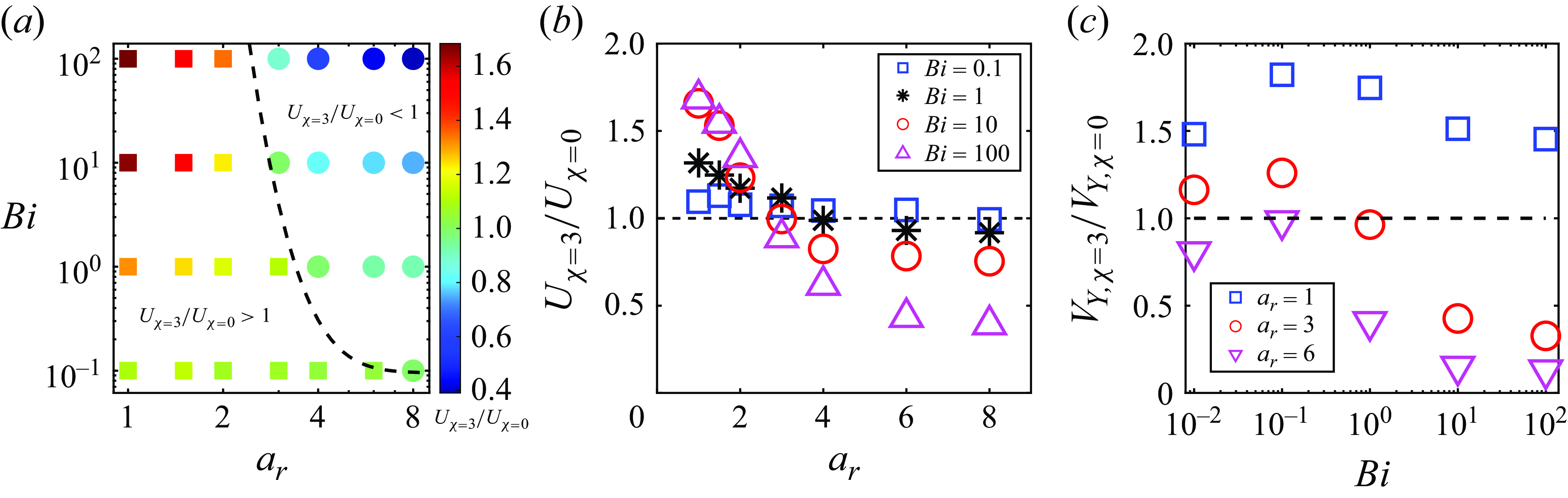
Figure 11. Ratio of swimming speed between a swirling squirmer ( $\chi =3$
) and a non-swirling neutral squirmer in a viscoplastic fluid. (a) Phase diagram over the aspect ratio
$\chi =3$
) and a non-swirling neutral squirmer in a viscoplastic fluid. (a) Phase diagram over the aspect ratio $a_r$
and Bingham number
$a_r$
and Bingham number $Bi$
. Symbols are coloured by the speed ratio
$Bi$
. Symbols are coloured by the speed ratio $U_{\chi =3}/U_{\chi =0}$
, and the dashed line gives the boundary between these states by data fitting. (b) Value of
$U_{\chi =3}/U_{\chi =0}$
, and the dashed line gives the boundary between these states by data fitting. (b) Value of $U_{\chi =3}/U_{\chi =0}$
as a function of the aspect ratio. (c) Normalised volume of yielded region
$U_{\chi =3}/U_{\chi =0}$
as a function of the aspect ratio. (c) Normalised volume of yielded region $V_{Y,\chi =3}/V_{Y,\chi =0}$
as a function of the Bingham number.
$V_{Y,\chi =3}/V_{Y,\chi =0}$
as a function of the Bingham number.
The stress distributions in figures 12 and 13 for $a_r=1.5$
and 6 can help us to understand the observed dependence of the yielded region on the swirling mode. In the case of
$a_r=1.5$
and 6 can help us to understand the observed dependence of the yielded region on the swirling mode. In the case of $a_r=1.5$
and
$a_r=1.5$
and $Bi=10$
, the magnitude of both normal and shear stresses around a swirling squirmer is much larger than that around a non-swirling squirmer, as shown in figure 12. Therefore, the yielded region around a swirling squirmer is larger than that around a non-swirling squirmer. Unlike the case of
$Bi=10$
, the magnitude of both normal and shear stresses around a swirling squirmer is much larger than that around a non-swirling squirmer, as shown in figure 12. Therefore, the yielded region around a swirling squirmer is larger than that around a non-swirling squirmer. Unlike the case of $a_r=1.5$
and
$a_r=1.5$
and $Bi=10$
, for the case of
$Bi=10$
, for the case of $a_r=6$
and
$a_r=6$
and $Bi=100$
, the magnitude of both normal and shear stresses around a swirling squirmer is smaller than that around a non-swirling squirmer, as shown in figure 13, resulting in a reduced yielded region for the swirling squirmer. The mechanism by which the swirling mode reduces stress around a squirmer with a large aspect ratio remains unclear and warrants further investigation.
$Bi=100$
, the magnitude of both normal and shear stresses around a swirling squirmer is smaller than that around a non-swirling squirmer, as shown in figure 13, resulting in a reduced yielded region for the swirling squirmer. The mechanism by which the swirling mode reduces stress around a squirmer with a large aspect ratio remains unclear and warrants further investigation.
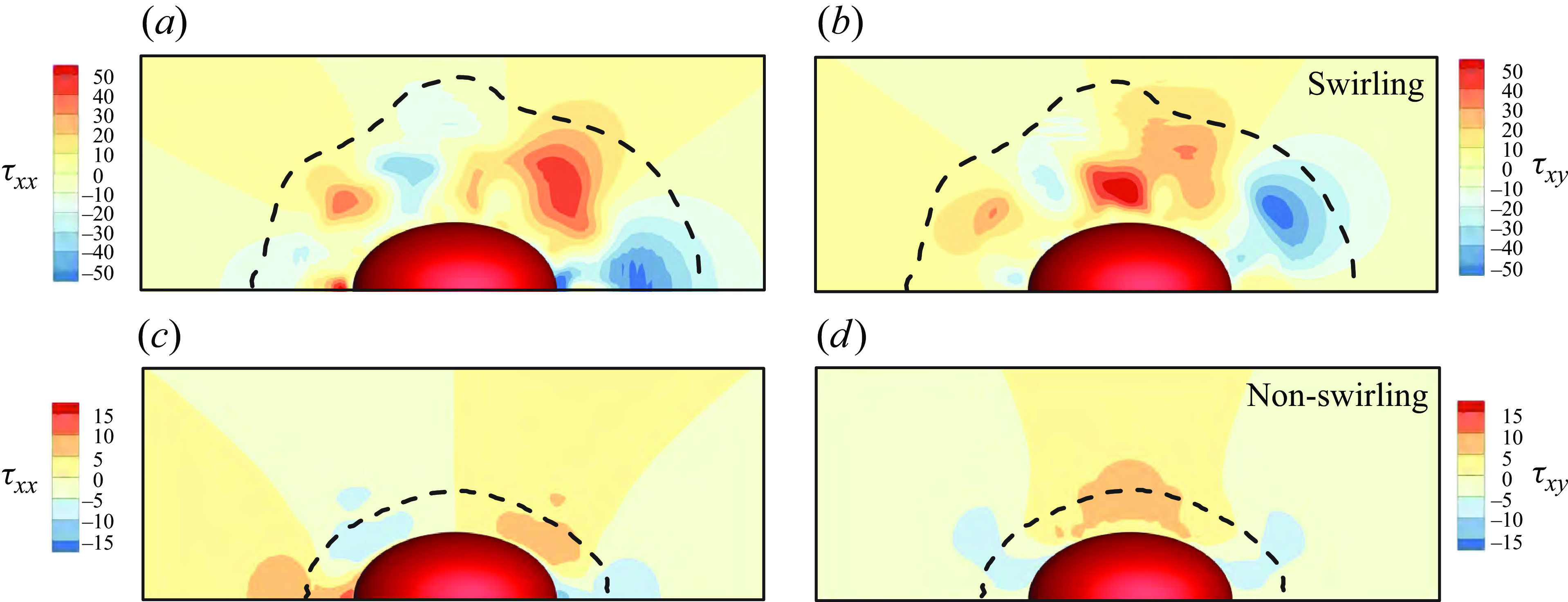
Figure 12. Stress fields around the squirmer ( $a_r=1.5$
) in a viscoplastic fluid with
$a_r=1.5$
) in a viscoplastic fluid with $Bi=10$
in the
$Bi=10$
in the $x$
–
$x$
– $y$
plane: (a,b) swirling swimmer
$y$
plane: (a,b) swirling swimmer $(\chi =3)$
and (c,d) non-swirling swimmer. Panels (a,c) show the normal stress
$(\chi =3)$
and (c,d) non-swirling swimmer. Panels (a,c) show the normal stress $\tau _{xx}$
, and panels (b,d) show the shear stress
$\tau _{xx}$
, and panels (b,d) show the shear stress $\tau _{xy}$
. The dashed line represents the yield surface.
$\tau _{xy}$
. The dashed line represents the yield surface.
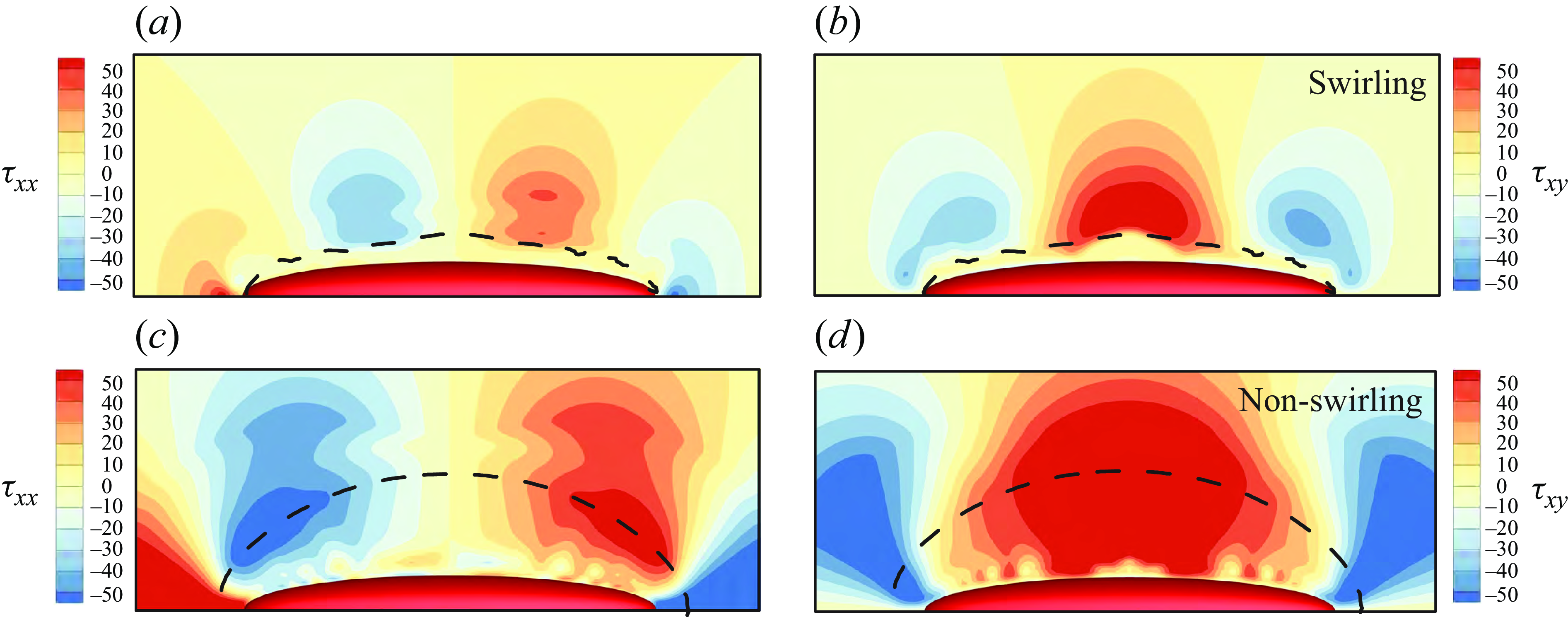
Figure 13. Stress fields around the squirmer ( $a_r=6$
) in a viscoplastic fluid with
$a_r=6$
) in a viscoplastic fluid with $Bi=100$
in the
$Bi=100$
in the $x$
–
$x$
– $y$
plane: (a,b) swirling swimmer
$y$
plane: (a,b) swirling swimmer $(\chi =3)$
and (c,d) non-swirling swimmer. Panels (a,c) show the normal stress
$(\chi =3)$
and (c,d) non-swirling swimmer. Panels (a,c) show the normal stress $\tau _{xx}$
, and panels (b,d) show the shear stress
$\tau _{xx}$
, and panels (b,d) show the shear stress $\tau _{xy}$
. The dashed line represents the yield surface.
$\tau _{xy}$
. The dashed line represents the yield surface.
3.4. Force analysis
The dimensionless net force acting on a force-free squirmer is given by
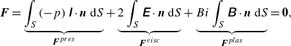 \begin{equation} \boldsymbol{F} = \underbrace {\int _S {\left ( { - p} \right){\unicode{x1D644}} \cdot {\boldsymbol{n}}\ {\textrm {d}}S} }_{{{\boldsymbol{F}}^{pres}}} + \underbrace {2\int _S {\unicode{x1D640}} \cdot {\boldsymbol{n}}\ {\textrm {d}}S}_{{{\boldsymbol{F}}^{visc}}} + \underbrace {{Bi}\int _S {{\unicode{x1D63D}} \cdot {\boldsymbol{n}}\ {\textrm {d}}S} }_{{{\boldsymbol{F}}^{plas}}} = {\boldsymbol{0}}, \end{equation}
where $\boldsymbol{F}^{pres}$
is the contribution due to pressure,
$\boldsymbol{F}^{pres}$
is the contribution due to pressure, $\boldsymbol{F}^{visc}$
results from the viscous stress and
$\boldsymbol{F}^{visc}$
results from the viscous stress and $\boldsymbol{F}^{plas}$
represents the plastic force.
$\boldsymbol{F}^{plas}$
represents the plastic force.
In a Newtonian fluid, the force can also be decomposed into contributions of the thrust force and towing force as $\boldsymbol{F}={\boldsymbol{F}_{thrust}} + {\boldsymbol{F}_{tow}} = 0$
. Here,
$\boldsymbol{F}={\boldsymbol{F}_{thrust}} + {\boldsymbol{F}_{tow}} = 0$
. Here, $\boldsymbol{F}_{thrust}$
is the thrust force generated by the squirmer when it is being held fixed, while
$\boldsymbol{F}_{thrust}$
is the thrust force generated by the squirmer when it is being held fixed, while ${\boldsymbol{F}_{tow}}=\alpha \boldsymbol{U}$
is the towing force required to tow the squirmer at the swimming speed
${\boldsymbol{F}_{tow}}=\alpha \boldsymbol{U}$
is the towing force required to tow the squirmer at the swimming speed $\boldsymbol{U}$
with
$\boldsymbol{U}$
with $\alpha$
being the translational drag coefficient (Yang et al. Reference Yang, Lu, Zhao, Kawamura and Chalmers2017). However, this decomposition in complex fluids is not entirely rigorous due to the nonlinearity of the rheology, i.e.
$\alpha$
being the translational drag coefficient (Yang et al. Reference Yang, Lu, Zhao, Kawamura and Chalmers2017). However, this decomposition in complex fluids is not entirely rigorous due to the nonlinearity of the rheology, i.e. $\boldsymbol{F}\ne {\boldsymbol{F}_{thrust}} + {\boldsymbol{F}_{tow}}$
, as discussed in Datt et al. (Reference Datt, Zhu, Elfring and Pak2015). We have carefully compared the thrust and towing forces in our settings and found that the difference between them is approximately 10 % in magnitude at
$\boldsymbol{F}\ne {\boldsymbol{F}_{thrust}} + {\boldsymbol{F}_{tow}}$
, as discussed in Datt et al. (Reference Datt, Zhu, Elfring and Pak2015). We have carefully compared the thrust and towing forces in our settings and found that the difference between them is approximately 10 % in magnitude at $Bi=10$
. Although such a decomposition is no longer rigorous in a viscoplastic fluid, we can still gain some insight into the propulsion behaviour by analysing the trust and drag forces separately. In particular, the comparison of the contributions of pressure, viscosity and plasticity and the comparison of the contributions of thrust and drag coefficients are helpful to facilitate our qualitative understanding.
$Bi=10$
. Although such a decomposition is no longer rigorous in a viscoplastic fluid, we can still gain some insight into the propulsion behaviour by analysing the trust and drag forces separately. In particular, the comparison of the contributions of pressure, viscosity and plasticity and the comparison of the contributions of thrust and drag coefficients are helpful to facilitate our qualitative understanding.
In this subsection, we discuss changes in the thrust forces that act to generate propulsion of the squirmer and how they vary with aspect ratio. This is done by analysing the force contributions parallel to the swimming axis on a fixed squirmer. Figure 14(a–c) illustrates the variation of the decomposed thrust forces as a function of the aspect ratio for different swimmer types at $Bi=10$
. We find that the total thrust forces do not change much for various aspect ratios, suggesting that the variation in free-swimming speed,
$Bi=10$
. We find that the total thrust forces do not change much for various aspect ratios, suggesting that the variation in free-swimming speed, $U$
, is primarily attributed to changes in swimming drag associated with squirmer’s aspect ratio. Moreover, the viscous, plastic and pressure contributions reveal a strong dependence on the cell shape. For all swimmer types, the viscous and plastic forces significantly increase with the aspect ratio, while the pressure force shows a decrease with
$U$
, is primarily attributed to changes in swimming drag associated with squirmer’s aspect ratio. Moreover, the viscous, plastic and pressure contributions reveal a strong dependence on the cell shape. For all swimmer types, the viscous and plastic forces significantly increase with the aspect ratio, while the pressure force shows a decrease with $a_r$
. By comparing figure 14(a–c), we observe that the neutral squirmer generates a larger thrust force than the puller/pusher or swirling squirmer. In figure 14(d), we provide the translational drag coefficient
$a_r$
. By comparing figure 14(a–c), we observe that the neutral squirmer generates a larger thrust force than the puller/pusher or swirling squirmer. In figure 14(d), we provide the translational drag coefficient $\alpha ={F}_{tow}/{U}$
, which decreases with the aspect ratio. Meanwhile, in figure 14(e), we observe that the volume of the yielded region around the fixed squirmer increases with the aspect ratio. This is because the reduction in the confinement effect causes a decrease in the translational drag coefficient as the aspect ratio increases. This ultimately leads to a higher swimming speed as the aspect ratio increases.
$\alpha ={F}_{tow}/{U}$
, which decreases with the aspect ratio. Meanwhile, in figure 14(e), we observe that the volume of the yielded region around the fixed squirmer increases with the aspect ratio. This is because the reduction in the confinement effect causes a decrease in the translational drag coefficient as the aspect ratio increases. This ultimately leads to a higher swimming speed as the aspect ratio increases.
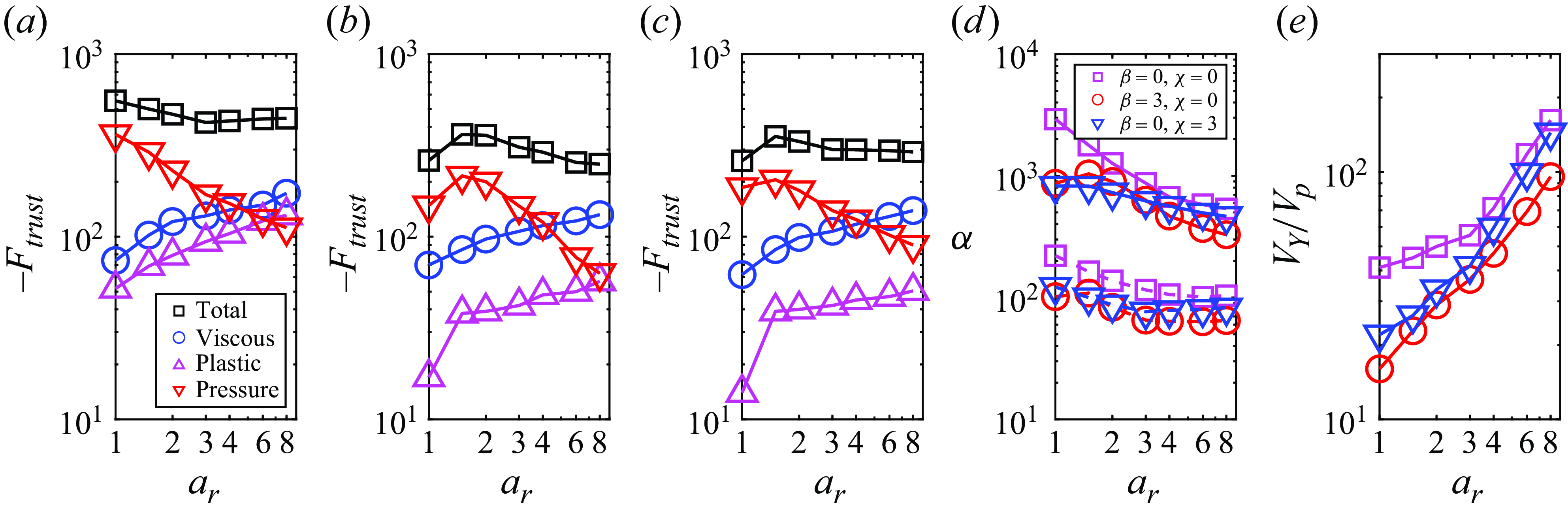
Figure 14. (a–c) Thrust force contributions as a function of aspect ratio at $Bi=10$
. Panel (a) neutral swimmer,
$Bi=10$
. Panel (a) neutral swimmer, $\beta =\chi =0$
, panel (b) puller,
$\beta =\chi =0$
, panel (b) puller, $\beta =3, \chi =0$
, panel (c) neutral swirling swimmer,
$\beta =3, \chi =0$
, panel (c) neutral swirling swimmer, $\beta =0,\chi =3$
. (d) Translational drag coefficient of different type of squirmers versus aspect ratio. The forces are normalised by
$\beta =0,\chi =3$
. (d) Translational drag coefficient of different type of squirmers versus aspect ratio. The forces are normalised by $\mu B_1 r_{eq}$
. (e) Volume of yielded region of squirmers versus aspect ratio.
$\mu B_1 r_{eq}$
. (e) Volume of yielded region of squirmers versus aspect ratio.
For a neutral squirmer with constant-volume constraints, the results in figure 14 are quite different from the observed behaviour in heterogeneous media (Demir et al. Reference Demir, van Gogh, Palaniappan and Nganguia2024). In heterogeneous fluids, the thrust force increases with the aspect ratio, and the drag coefficient shows a non-monotonic trend as a function of the aspect ratio: $\alpha$
generally increases with increasing the aspect ratio for
$\alpha$
generally increases with increasing the aspect ratio for $a_r \gt 2.3$
. In summary, the increase in swimming speed with aspect ratio in a heterogeneous fluid is primarily attributed to the enhanced thrust force, whereas in a viscoplastic fluid, the increase in swimming speed results from a decrease in the drag coefficient.
$a_r \gt 2.3$
. In summary, the increase in swimming speed with aspect ratio in a heterogeneous fluid is primarily attributed to the enhanced thrust force, whereas in a viscoplastic fluid, the increase in swimming speed results from a decrease in the drag coefficient.
4. Squirmer-induced diffusion
Fluid particle diffusion induced by swimmers is a crucial factor in enhancing mass transport and nutrient uptake, and is thus linked to a wide variety of biological phenomena, such as reproduction, colonisation and infection. In the dilute limit, where swimmers move along straight paths and the interactions between tracers and swimmers are well captured, the diffusivity of fluid particle (tracer) is well studied (Thiffeault & Childress Reference Thiffeault and Childress2010; Lin et al. Reference Lin, Thiffeault and Childress2011; Pushkin & Yeomans Reference Pushkin and Yeomans2013; Pushkin et al. Reference Pushkin, Shum and Yeomans2013; Mueller & Thiffeault Reference Mueller and Thiffeault2017). While the enhanced diffusion due to swimmers has been extensively explored, the combined effects of the swimmer shape and the rheological properties of the surrounding fluid on the diffusive properties of fluid particles remain inadequately understood. Our aim here is to explore how both the squirmer shape and the fluid viscoplasticity influence the diffusion phenomena.
4.1. Motion of fluid particles
As depicted in figure 15(a), we consider an axially symmetric squirmer that moves in a straight line along the $x$
direction with a constant velocity
$x$
direction with a constant velocity $U$
in a viscoplastic fluid. Here,
$U$
in a viscoplastic fluid. Here, $L_x$
,
$L_x$
, $L_y$
and
$L_y$
and $L_z$
represent the domain sizes in the
$L_z$
represent the domain sizes in the $x$
,
$x$
, $y$
and
$y$
and $z$
directions, respectively. We define
$z$
directions, respectively. We define $A=L_yL_z$
as the cross-sectional area of the region, which is equal to
$A=L_yL_z$
as the cross-sectional area of the region, which is equal to $ ( 32r_{eq})^2$
. The simulation is carried out to the extent that this cross-sectional area is larger than the yielded region. The area farther away from this region is solidified by plasticity, so the motion of the fluid particles, including Brownian motion, is assumed to be negligible.
$ ( 32r_{eq})^2$
. The simulation is carried out to the extent that this cross-sectional area is larger than the yielded region. The area farther away from this region is solidified by plasticity, so the motion of the fluid particles, including Brownian motion, is assumed to be negligible.
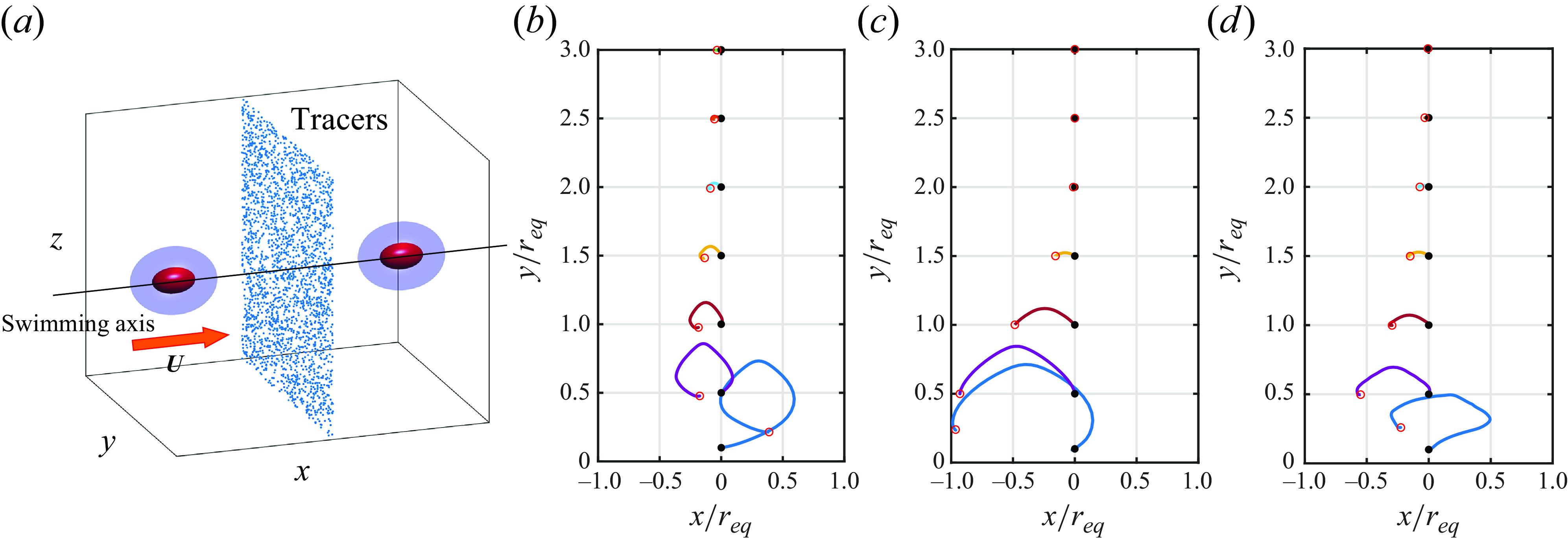
Figure 15. (a) Numerical settings for the calculation of squirmer-induced diffusion. (b–d) Typical trajectories of tracers as a neutral squirmer moves along the $x$
axis. Panel (b),
$x$
axis. Panel (b), $a_r=3,Bi=0.01$
; (c)
$a_r=3,Bi=0.01$
; (c) $a_r=3,Bi=1.0$
; (d)
$a_r=3,Bi=1.0$
; (d) $a_r=8,Bi=1.0$
. The starting and ending points of the tracer trajectories are marked by filled black circles and open red circles, respectively. Here,
$a_r=8,Bi=1.0$
. The starting and ending points of the tracer trajectories are marked by filled black circles and open red circles, respectively. Here, $y=0$
represents the swimming axis of the squirmer.
$y=0$
represents the swimming axis of the squirmer.
The number of sample tracers used in the simulation is $N=1000^2$
, and their initial positions,
$N=1000^2$
, and their initial positions, ${\boldsymbol{r}}_i^{initial}$
, are set uniformly at random in the mid-plane, where the flow is initially unyielded. After the squirmer passes away, the sample tracers move to
${\boldsymbol{r}}_i^{initial}$
, are set uniformly at random in the mid-plane, where the flow is initially unyielded. After the squirmer passes away, the sample tracers move to ${\boldsymbol{r}}_i^{final}$
in the unyielded region and stop moving. Particles are assumed to move with the velocity created by the squirmer and the effect of Brownian motion is ignored. The displacement of the
${\boldsymbol{r}}_i^{final}$
in the unyielded region and stop moving. Particles are assumed to move with the velocity created by the squirmer and the effect of Brownian motion is ignored. The displacement of the $i$
th tracer is defined as
$i$
th tracer is defined as $\Delta {{\boldsymbol{r}}_i} = {{\boldsymbol{r}}_i^{final}} - {\boldsymbol{r}}_i^{initial}$
, and the ensemble-averaged squared displacement tensor can be calculated by
$\Delta {{\boldsymbol{r}}_i} = {{\boldsymbol{r}}_i^{final}} - {\boldsymbol{r}}_i^{initial}$
, and the ensemble-averaged squared displacement tensor can be calculated by
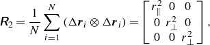 \begin{equation} {\unicode{x1D64D}}_2 = \frac {1}{N}\sum \limits _{i = 1}^N {\left ( {\Delta {{\boldsymbol{r}}_i} \otimes \Delta {{\boldsymbol{r}}_i}} \right)} = \left [ {\begin{array}{*{20}{c}} {r_\parallel ^2}&0&0\\ 0&r_ \bot ^2&0\\ 0&0&r_ \bot ^2 \end{array}} \right], \end{equation}
where $r_\parallel$
and
$r_\parallel$
and $r_ \bot$
are the average displacements over the
$r_ \bot$
are the average displacements over the $N$
tracers parallel to (longitudinal), and in the plane perpendicular to (transverse), the swimming direction. The velocities of the tracers are interpolated from the velocity fields, and the time integration is performed using a second-order Runge–Kutta method. The accuracy of the calculated displacements is guaranteed by the number of particles and the database resolution used in this study. The representative trajectories of the tracer particles for specific cases (
$N$
tracers parallel to (longitudinal), and in the plane perpendicular to (transverse), the swimming direction. The velocities of the tracers are interpolated from the velocity fields, and the time integration is performed using a second-order Runge–Kutta method. The accuracy of the calculated displacements is guaranteed by the number of particles and the database resolution used in this study. The representative trajectories of the tracer particles for specific cases ( $\beta =0$
) are shown in figure 15(b–d). At a low Bingham number of
$\beta =0$
) are shown in figure 15(b–d). At a low Bingham number of $Bi=0.01$
, the tracers initially positioned near the swimming axis tend to move forward, while those farther from the axis are displaced backwards. In contrast, at
$Bi=0.01$
, the tracers initially positioned near the swimming axis tend to move forward, while those farther from the axis are displaced backwards. In contrast, at $Bi=1$
, all tracers are displaced backwards. In general, the longitudinal average squared displacement
$Bi=1$
, all tracers are displaced backwards. In general, the longitudinal average squared displacement $r^2_\parallel$
dominates over the transverse average squared displacement
$r^2_\parallel$
dominates over the transverse average squared displacement $r^2_ \bot$
, hence we focus on the longitudinal squared displacement in the following discussion.
$r^2_ \bot$
, hence we focus on the longitudinal squared displacement in the following discussion.
Figure 16 presents the scaled longitudinal average displacement, ${r_\parallel ^2}/r^2_{eq}$
, as a function of
${r_\parallel ^2}/r^2_{eq}$
, as a function of $a_r$
and
$a_r$
and $Bi$
. Figure 16(a) reveals that, when the aspect ratio exceeds 2,
$Bi$
. Figure 16(a) reveals that, when the aspect ratio exceeds 2, $r^2_\parallel$
decreases as the aspect ratio increases. This can be understood by comparing the tracer trajectories in figure 15(c,d) for a neutral squirmer (
$r^2_\parallel$
decreases as the aspect ratio increases. This can be understood by comparing the tracer trajectories in figure 15(c,d) for a neutral squirmer ( $Bi=1$
,
$Bi=1$
, $a_r=3$
and 8) in motion. As the aspect ratio increases, a decrease in the backward displacement is observed for tracers initially positioned near the swimming axis, leading to a reduction in the longitudinal average squared displacement. In figure 16(b), we find that
$a_r=3$
and 8) in motion. As the aspect ratio increases, a decrease in the backward displacement is observed for tracers initially positioned near the swimming axis, leading to a reduction in the longitudinal average squared displacement. In figure 16(b), we find that $r^2_\parallel$
generally increases with the Bingham number. As presented in figure 15(b,c), an increase in the backward displacement of tracers is observed as
$r^2_\parallel$
generally increases with the Bingham number. As presented in figure 15(b,c), an increase in the backward displacement of tracers is observed as $Bi$
increases, then the longitudinal average squared displacement increases.
$Bi$
increases, then the longitudinal average squared displacement increases.
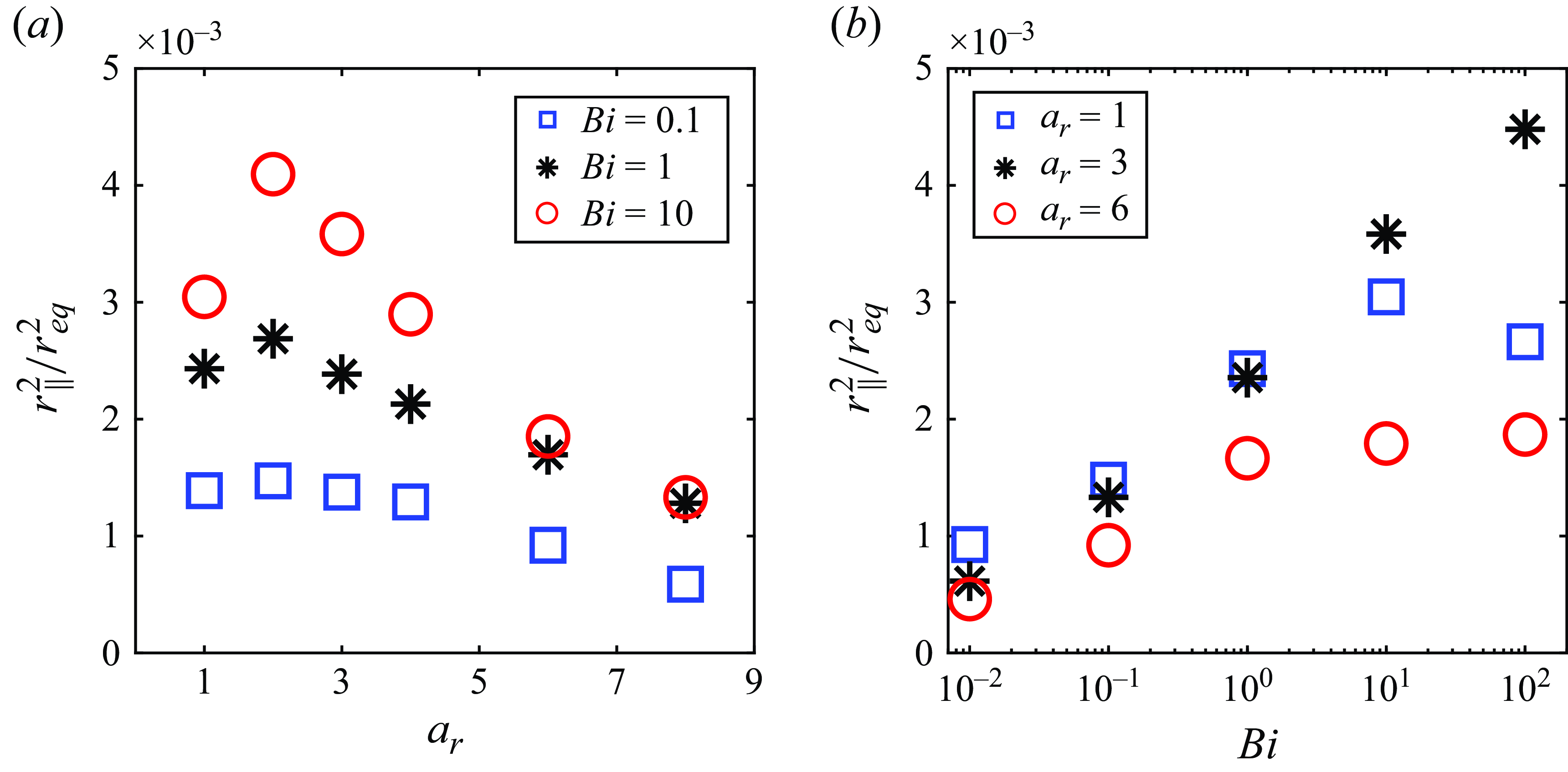
Figure 16. Dependence of the scaled longitudinal average displacement, ${r_\parallel ^2}/r^2_{eq}$
, on (a) the aspect ratio and (b) the Bingham number for a neutral squirmer.
${r_\parallel ^2}/r^2_{eq}$
, on (a) the aspect ratio and (b) the Bingham number for a neutral squirmer.
4.2. Diffusion coefficient
The diffusivity is a measure of the spreading of the tracer particles. The definition of the diffusion tensor is given by
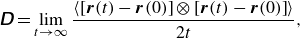 \begin{equation} \unicode{x1D63F} = \lim _{t \rightarrow \infty } \frac {\langle \left [\boldsymbol{r}(t)-\boldsymbol{r}(0)\right] \otimes \left [\boldsymbol{r}(t)-\boldsymbol{r}(0)\right]\rangle }{2t}, \end{equation}
where $\boldsymbol{r}$
is the position of a fluid particle, and the angle bracket denotes an ensemble average over particles in the whole domain.
$\boldsymbol{r}$
is the position of a fluid particle, and the angle bracket denotes an ensemble average over particles in the whole domain.
Here, we focus on fluid particle diffusion in a dilute suspension of squirmers, allowing us to neglect multi-body interactions of squirmers. Since the motion of tracers in a plastic fluid is restricted to the vicinity of the squirmer, the tracer particles only move when a swimmer comes close and otherwise remain stationary. Furthermore, we assume an isotropic suspension, where the orientation of the squirmers is isotropic. Under these assumptions, the tracer exhibits a three-dimensional random walk, taking steps only when the squirmer comes close. The diffusion tensor becomes isotropic, and given by
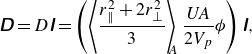 \begin{equation} \unicode{x1D63F} = D \unicode{x1D644} = \left ( \left \langle \frac {r_\parallel ^2 + 2 r_ \bot ^2}{3} \right \rangle _{\! \! \! A} \frac {U \! A}{2 V_p} \phi \right) \unicode{x1D644}, \end{equation}
where $\langle \ \rangle _{\! A}$
indicates the average over the cross-sectional area
$\langle \ \rangle _{\! A}$
indicates the average over the cross-sectional area $A$
, and
$A$
, and $\phi$
is the volume fraction of squirmers in a dilute suspension. This definition indicates that the diffusivity is linearly related to the total squared displacement of tracers, the swimming speed
$\phi$
is the volume fraction of squirmers in a dilute suspension. This definition indicates that the diffusivity is linearly related to the total squared displacement of tracers, the swimming speed $U$
and the volume fraction
$U$
and the volume fraction $\phi$
.
$\phi$
.
Figure 17 shows the numerically calculated squirmer-induced diffusivity, $D$
, as a function of
$D$
, as a function of $a_r$
and
$a_r$
and $Bi$
. The results reveal a non-monotonic behaviour of diffusivity with respect to both the aspect ratio and the Bingham number. As these parameters increase, the diffusivity first reaches a maximum and then decreases. The increase in
$Bi$
. The results reveal a non-monotonic behaviour of diffusivity with respect to both the aspect ratio and the Bingham number. As these parameters increase, the diffusivity first reaches a maximum and then decreases. The increase in $D$
with
$D$
with $a_r$
in figure 17(a) is attributed to the increase in swimming speed shown in figure 3(a), while the decrease in
$a_r$
in figure 17(a) is attributed to the increase in swimming speed shown in figure 3(a), while the decrease in $D$
with further increased
$D$
with further increased $a_r$
results from the reduction in the average squared displacement in figure 16(a). In contract, the increase in
$a_r$
results from the reduction in the average squared displacement in figure 16(a). In contract, the increase in $D$
with
$D$
with $Bi$
for
$Bi$
for $Bi \leqslant 1$
is driven by the increase in the average squared displacement, while the decrease in
$Bi \leqslant 1$
is driven by the increase in the average squared displacement, while the decrease in $D$
with
$D$
with $Bi$
at higher Bingham numbers is due to the reduced swimming speed, as seen in figure 2(a).
$Bi$
at higher Bingham numbers is due to the reduced swimming speed, as seen in figure 2(a).
We then investigated the effect of the swimming dipolarity $\beta$
(
$\beta$
( $\left | \beta \right | \leqslant 1$
) on the squirmer-induced diffusivity
$\left | \beta \right | \leqslant 1$
) on the squirmer-induced diffusivity $D$
. As shown in figure 18, we see that both
$D$
. As shown in figure 18, we see that both $r_\parallel ^2$
and
$r_\parallel ^2$
and $D$
reach minimum values when
$D$
reach minimum values when $\beta =0$
, i.e. for neutral squirmer, and increase as
$\beta =0$
, i.e. for neutral squirmer, and increase as $\left | \beta \right |$
increased. This result is qualitatively consistent with previous studies for a Newtonian fluid (Pushkin et al. Reference Pushkin, Shum and Yeomans2013; Thiffeault Reference Thiffeault2015). Figure 19 shows the representative trajectories of tracer particles for the spherical cases (
$\left | \beta \right |$
increased. This result is qualitatively consistent with previous studies for a Newtonian fluid (Pushkin et al. Reference Pushkin, Shum and Yeomans2013; Thiffeault Reference Thiffeault2015). Figure 19 shows the representative trajectories of tracer particles for the spherical cases ( $a_r=1$
and
$a_r=1$
and $Bi=0.1$
). As
$Bi=0.1$
). As $\left | \beta \right |$
increases, the tracers initially positioned near the swimming axis tend to move forward with larger displacement, thereby enhancing the average longitudinal squared displacement and diffusivity.
$\left | \beta \right |$
increases, the tracers initially positioned near the swimming axis tend to move forward with larger displacement, thereby enhancing the average longitudinal squared displacement and diffusivity.
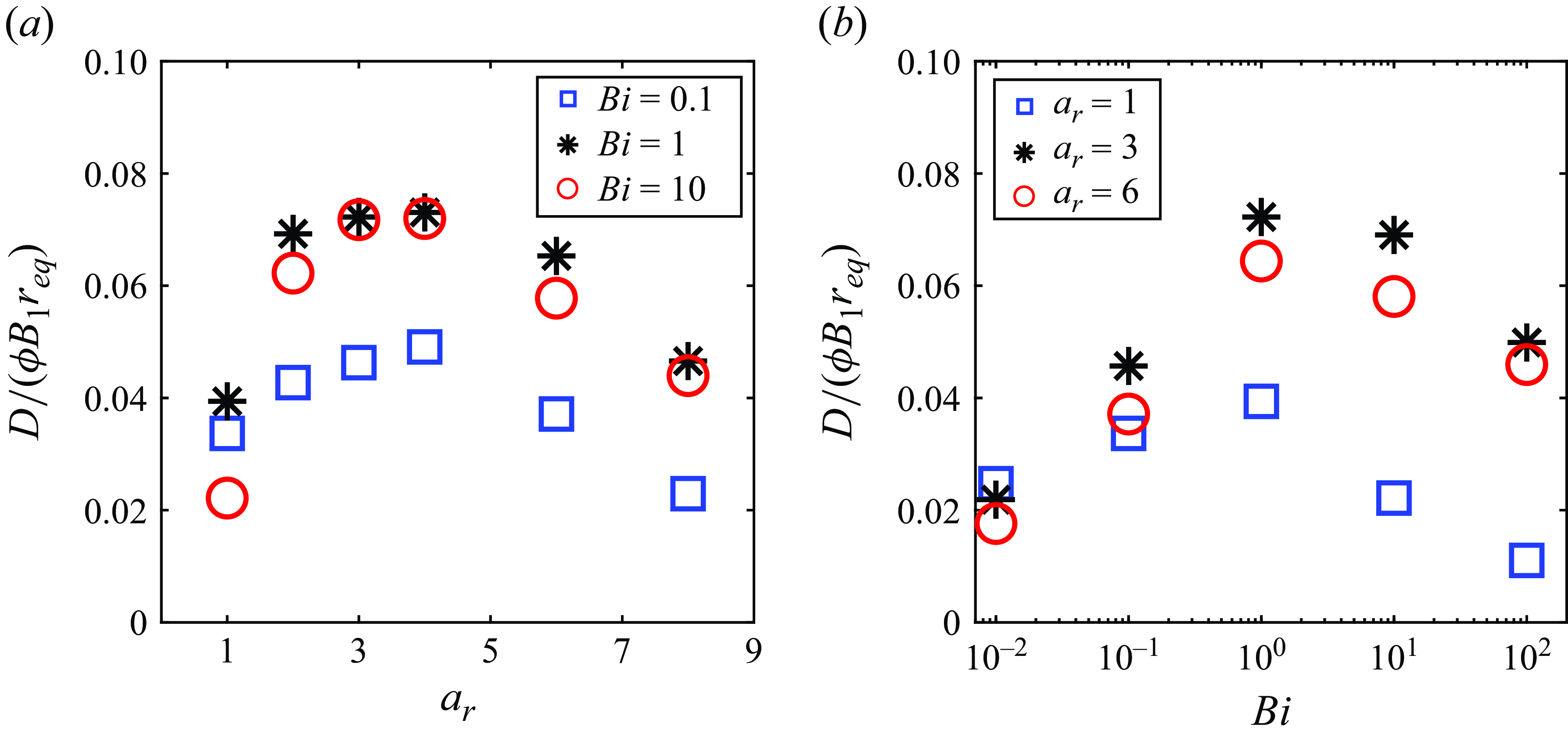
Figure 17. Dependence of squirmer-induced diffusivity on (a) the aspect ratio and (b) the Bingham number for a neutral squirmer.
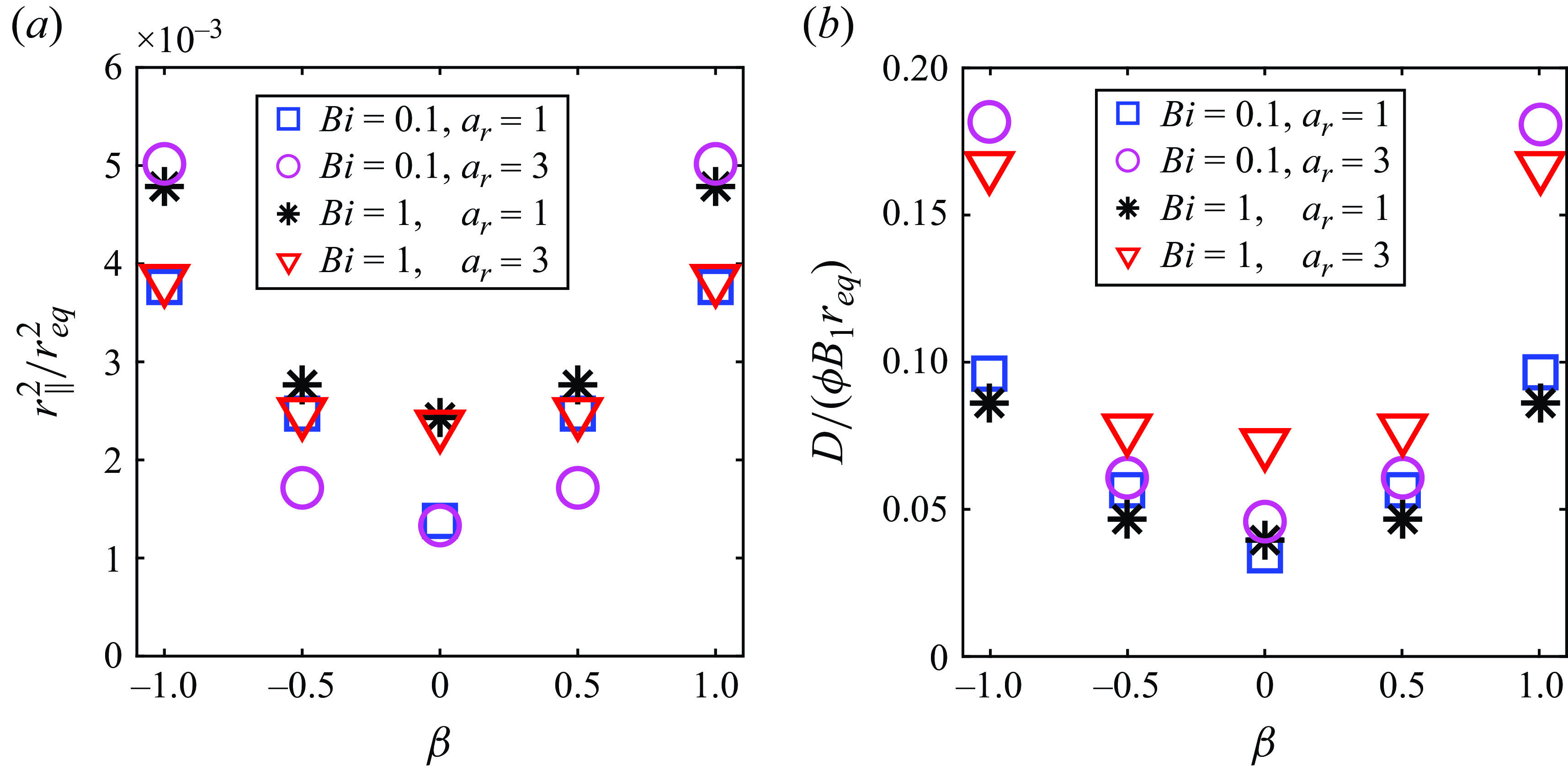
Figure 18. Effect of $\beta$
on (a) the longitudinal average displacement and (b) the squirmer-induced diffusivity.
$\beta$
on (a) the longitudinal average displacement and (b) the squirmer-induced diffusivity.
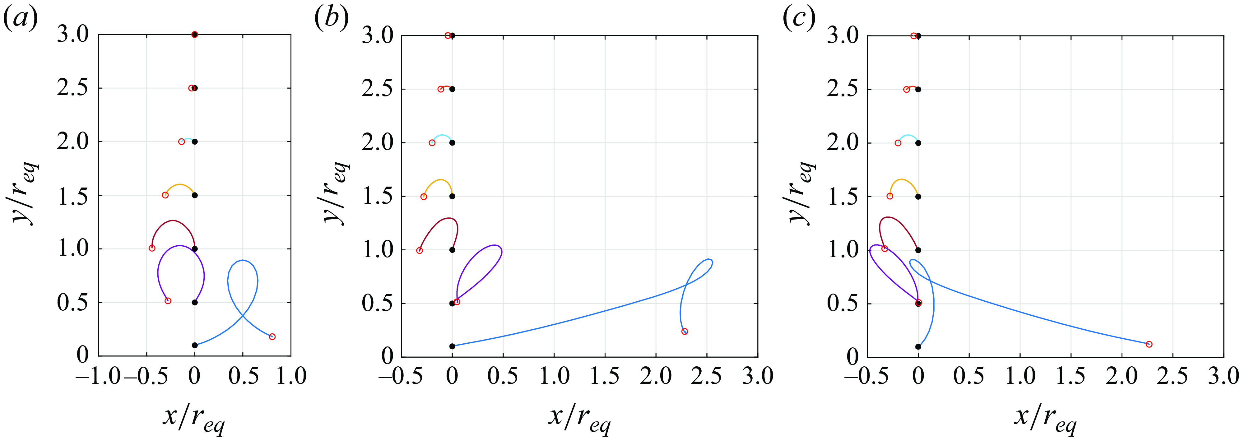
Figure 19. Typical trajectories of tracers as a squirmer ( $a_r=1$
and
$a_r=1$
and $Bi=0.1$
) moves along the
$Bi=0.1$
) moves along the $x$
axis. Panel (a)
$x$
axis. Panel (a) $\beta =0$
; (b)
$\beta =0$
; (b) $\beta =-1$
; (c)
$\beta =-1$
; (c) $\beta =1$
. The starting and ending points of the tracer paths are marked by filled black circles and open red circles, respectively.
$\beta =1$
. The starting and ending points of the tracer paths are marked by filled black circles and open red circles, respectively.
5. Conclusion
In this study, we numerically investigated the impact of fluid viscoplasticity and microswimmer body shape on locomotion and swimmer-induced diffusion.
Our results show that both spherical and ellipsoidal neutral squirmers experience reduced speed and increased power dissipation as the Bingham number $Bi$
increases. The efficiency of the swimmer, on the other hand, reaches its highest value at a moderate range of
$Bi$
increases. The efficiency of the swimmer, on the other hand, reaches its highest value at a moderate range of $Bi$
. By increasing the aspect ratio, ellipsoidal squirmers exhibit significantly faster swimming speeds over spherical squirmers in viscoplastic fluids. Moreover, ellipsoidal squirmers swim more efficiently in a weak viscoplastic fluid (
$Bi$
. By increasing the aspect ratio, ellipsoidal squirmers exhibit significantly faster swimming speeds over spherical squirmers in viscoplastic fluids. Moreover, ellipsoidal squirmers swim more efficiently in a weak viscoplastic fluid ( $Bi \leqslant 10^{-1}$
), but less efficiently under stronger viscoplastic conditions compared with spherical squirmers. This behaviour is attributed to the reduced confinement effect from the yield surface for elongated squirmers. We found that, for a fixed
$Bi \leqslant 10^{-1}$
), but less efficiently under stronger viscoplastic conditions compared with spherical squirmers. This behaviour is attributed to the reduced confinement effect from the yield surface for elongated squirmers. We found that, for a fixed $Bi$
, the ellipsoidal squirmer induces a larger yielded region than the spherical squirmer, particularly at high Bingham numbers.
$Bi$
, the ellipsoidal squirmer induces a larger yielded region than the spherical squirmer, particularly at high Bingham numbers.
The swimming speed of the squirmer can be either enhanced or diminished by including the second polar mode or swirling mode, depending on the combined effects of the Bingham number and aspect ratio. We found that pullers and pushers with the same strength of dipolarity have indistinguishable swimming speeds and efficiencies. Below a critical aspect ratio or Bingham number, the speed of a puller/pusher or swirling squirmer exceeds that of its neutral squirmer counterpart, but above the critical values, these modes slow down the squirmer. These findings highlight the importance of investigating squirming modes to optimise swimming strategies in viscoplastic fluids. We plan to explore the critical values over a broader parameter range in future work.
We examine how the thrust forces and translational drag coefficients vary as a function of the aspect ratio for different types of squirmers. Unlike the case of squirmers in heterogeneous media (Demir et al. Reference Demir, van Gogh, Palaniappan and Nganguia2024), we found that while the total thrust forces do not change significantly with varying aspect ratios, the translational drag coefficients exhibit a pronounced decrease as the aspect ratio increases. These findings help explain the increase in propulsion speed as a function of aspect ratio in a viscoplastic fluid.
The yield stress always restricts the flow region within a yield surface that lies at a finite distance from the squirmer, thereby influencing the diffusion of fluid particles in viscoplastic fluids. We calculated the squirmer-induced diffusivity and found that it is higher for moderate aspect ratios and Bingham numbers, increasing with the magnitude of the squirmer’s dipolarity. This study represents a first step towards understanding the enhanced diffusion caused by non-spherical swimmers in complex fluids. It suggests that a moderate aspect ratio of microswimmers, combined with the fluid viscoplasticity, can significantly enhance active mixing.
Recent studies have explored the propulsion of ellipsoidal squirmers in complex environments (van Gogh et al. Reference van Gogh, Demir, Palaniappan and Pak2022; Demir et al. Reference Demir, van Gogh, Palaniappan and Nganguia2024; Gong et al. Reference Gong, Shaik and Elfring2024). Our findings complement these closely related studies by addressing swimming in a viscoplastic Bingham fluid. We note that the Bingham material is the simplest viscoplastic fluid, neglecting viscoelastic and thixotropic effects seen in gel-like mucus. Future research could investigate the swimming behaviour of squirmers in more complex environments. Another intriguing avenue for future study is the impact of our findings on the hydrodynamic interactions between microswimmers in viscoplastic fluids. Since flow properties undergo rapid transitions across the yield surface, the collective motion of swimmers in such a fluid will differ significantly from that in Newtonian fluids or heterogeneous media.
Funding
The work was supported by the National Natural Science Foundation of China (grant nos. 12302340, 12172327, 12132015 and 12332015), and the Japan Society for the Promotion of Science Grant-in-Aid for Scientific Research (JSPS KAKENHI Grants Nos. 24KF0097, 21H04999 and 21H05308).
Declaration of interests
The authors report no conflict of interest.
Appendix A. Imposed solenoidal velocity
To recover the tangential velocity $\boldsymbol{u}_{sq}$
on the surface of the squirmer (given in (2.6)), we impose an internal velocity field
$\boldsymbol{u}_{sq}$
on the surface of the squirmer (given in (2.6)), we impose an internal velocity field $\boldsymbol{u}_a$
inside the squirmer. The value of
$\boldsymbol{u}_a$
inside the squirmer. The value of $\boldsymbol{u}_a$
on the surface of the squirmer satisfies
$\boldsymbol{u}_a$
on the surface of the squirmer satisfies
 \begin{equation} \left.\boldsymbol{u}_a \right |_{\tau =\tau _0}= {{\boldsymbol{u}}_{{{sq}}}} = -B_1 \tau _0(1-\zeta ^2)^{\frac {1}{2}}\big(\tau _0^2-\zeta ^2\big)^{-\frac {1}{2}}[(1+\beta \zeta) \boldsymbol{e}_\zeta +3 \chi \zeta \boldsymbol{e}_{\varphi }]. \end{equation}
The imposed flow leads to a zero translational and rotational velocity (Li & Ardekani Reference Li and Ardekani2014), i.e.
 \begin{equation} \iiint \boldsymbol{u}_a J {\textrm {d}} \zeta {\textrm {d}} \tau {\textrm {d}} \varphi = {0},\ \ {\textrm {and}}\ \ \iiint \boldsymbol{r} \times \boldsymbol{u}_a J {\textrm {d}} \zeta {\textrm {d}} \tau {\textrm {d}} \varphi = {0}, \end{equation}
where $J = h_\zeta h_\tau h_{\varphi }$
is the Jacobian determinant. In the spheroidal coordinate system, the internal flow can be decomposed into
$J = h_\zeta h_\tau h_{\varphi }$
is the Jacobian determinant. In the spheroidal coordinate system, the internal flow can be decomposed into $\boldsymbol{u}_{a1} = v_{\tau }\boldsymbol{e}_\tau +v_{\zeta }\boldsymbol{e}_\zeta$
and
$\boldsymbol{u}_{a1} = v_{\tau }\boldsymbol{e}_\tau +v_{\zeta }\boldsymbol{e}_\zeta$
and $\boldsymbol{u}_{a2} = v_{\varphi }\boldsymbol{e}_\varphi$
.
$\boldsymbol{u}_{a2} = v_{\varphi }\boldsymbol{e}_\varphi$
.
The axisymmetric flow $\boldsymbol{u}_{a1}$
can be expressed by the streamfunction
$\boldsymbol{u}_{a1}$
can be expressed by the streamfunction $\Psi (\tau, \zeta)$
as
$\Psi (\tau, \zeta)$
as $\boldsymbol{u}_{a1}=\operatorname {curl} ( \Psi (\tau, \zeta) \boldsymbol{e}_{\varphi }/{h_{\varphi }})$
, which satisfies
$\boldsymbol{u}_{a1}=\operatorname {curl} ( \Psi (\tau, \zeta) \boldsymbol{e}_{\varphi }/{h_{\varphi }})$
, which satisfies $E^4 \Psi (\tau, \zeta) = 0$
with
$E^4 \Psi (\tau, \zeta) = 0$
with
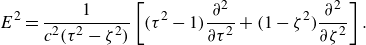 \begin{equation} E^2=\frac {1}{c^2 (\tau ^2-\zeta ^2)} \left[ (\tau ^2-1) \frac {\partial ^2}{\partial \tau ^2}+ (1-\zeta ^2) \frac {\partial ^2}{\partial \zeta ^2}\right]. \end{equation}
The velocity components of $\boldsymbol{u}_{a1}$
can be derived as
$\boldsymbol{u}_{a1}$
can be derived as
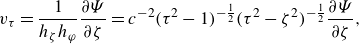 \begin{equation} v_{\tau }=\frac {1}{h_\zeta h_{\varphi }} \frac {\partial \Psi }{\partial \zeta }=c^{-2} (\tau ^2-1)^{-\frac {1}{2}} (\tau ^2-\zeta ^2)^{-\frac {1}{2}} \frac {\partial \Psi }{\partial \zeta }, \end{equation}
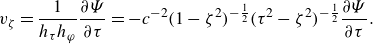 \begin{equation} v_{\zeta }=\frac {1}{h_\tau h_{\varphi }} \frac {\partial \Psi }{\partial \tau }=-c^{-2} (1-\zeta ^2)^{-\frac {1}{2}} (\tau ^2-\zeta ^2)^{-\frac {1}{2}} \frac {\partial \Psi }{\partial \tau }. \end{equation}
The general separable solution for the stream function can be obtained as (Dassios et al. Reference Dassios, Hadjinicolaou and Payatakes1994)
 \begin{equation} \Psi (\tau, \zeta)=g_0(\tau) G_0(\zeta)+g_1(\tau) G_1(\zeta)+\sum _{n=2}^{\infty } [g_n(\tau) G_n(\zeta)+h_n(\tau) H_n(\zeta)]. \end{equation}
Here, $G_n$
and
$G_n$
and $H_n$
are the Gegenbauer functions of the first and second kinds, respectively, while
$H_n$
are the Gegenbauer functions of the first and second kinds, respectively, while $g_n(\tau)$
and
$g_n(\tau)$
and $h_n(\tau)$
are
$h_n(\tau)$
are $\tau$
-dependent functions given by certain linear combinations of
$\tau$
-dependent functions given by certain linear combinations of $G_k(\tau)$
and
$G_k(\tau)$
and $H_k(\tau)$
. For our problem, (A6) can be simplified as
$H_k(\tau)$
. For our problem, (A6) can be simplified as $\Psi (\tau, \zeta)=g_2(\tau) G_2(\zeta)+g_3(\tau) G_3(\zeta)$
. The functions
$\Psi (\tau, \zeta)=g_2(\tau) G_2(\zeta)+g_3(\tau) G_3(\zeta)$
. The functions $g_2(\tau)$
and
$g_2(\tau)$
and $g_3(\tau)$
are determined as
$g_3(\tau)$
are determined as
 \begin{equation} g_2(\tau) =a_0 G_0(\tau)+a_1 G_1(\tau)+a_2 G_2(\tau)+a_3 G_4(\tau), \end{equation}
 \begin{equation} g_3(\tau) =a_4 G_0(\tau)+a_5 G_1(\tau)+a_6 G_3(\tau), \end{equation}
where the constants $a_k$
will be further calculated by requiring that the solution satisfies (A1) and (A2). The boundary conditions for
$a_k$
will be further calculated by requiring that the solution satisfies (A1) and (A2). The boundary conditions for $\Psi (\tau, \zeta)$
read
$\Psi (\tau, \zeta)$
read
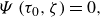 \begin{equation} \Psi \left (\tau _0, \zeta \right)=0, \end{equation}
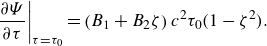 \begin{equation} \left.\frac {\partial \Psi }{\partial \tau }\right |_{\tau =\tau _0}=\left (B_1+B_2 \zeta \right) c^2 \tau _0(1-\zeta ^2). \end{equation}
Note that (A9) ensures $v_{\tau } = 0$
at the squirmer’s surface (Theers et al. Reference Theers, Westphal, Gompper and Winkler2016). Since (A9) and (A10) involve elliptic integrals, this boundary value problem is solved by numerical method, and we list the numerical solution of
$v_{\tau } = 0$
at the squirmer’s surface (Theers et al. Reference Theers, Westphal, Gompper and Winkler2016). Since (A9) and (A10) involve elliptic integrals, this boundary value problem is solved by numerical method, and we list the numerical solution of $a_k$
in table 3.
$a_k$
in table 3.


Assuming that $\boldsymbol{u}_{a2} = v_\varphi \boldsymbol{e}_\varphi$
is purely in the
$\boldsymbol{u}_{a2} = v_\varphi \boldsymbol{e}_\varphi$
is purely in the $\varphi$
direction with no
$\varphi$
direction with no $\varphi$
dependence, a specific velocity is given as
$\varphi$
dependence, a specific velocity is given as
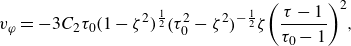 \begin{equation} {v_\varphi } = - 3{C_2}{\tau _0}{( {1 - {\zeta ^2}} )^{\frac {1}{2}}}{\big( {\tau _0^2 - {\zeta ^2}} \big)^{ - \frac {1}{2}}}\zeta {\left ( {\frac {{\tau - 1}}{{{\tau _0} - 1}}} \right)^2}, \end{equation}
which satisfies the boundary condition as well as the conditions of zero translational and rotational velocity
 \begin{equation} v_{\varphi }(\tau _0, \zeta )=-3C_2 \tau _0 (1-\zeta ^2)^{\frac {1}{2}} \big(\tau _0^2-\zeta ^2\big)^{-\frac {1}{2}} \zeta, \end{equation}
 \begin{equation} \iiint \boldsymbol{u}_{a2} J {\textrm {d}} \zeta {\textrm {d}} \tau {\textrm {d}} \varphi = {0}\quad {\textrm {and}}\quad \iiint \boldsymbol{r} \times \boldsymbol{u}_{a2} J {\textrm {d}} \zeta {\textrm {d}} \tau {\textrm {d}} \varphi = {0}. \end{equation}
We note that (A11) does not satisfy the Stokes equation. Nevertheless, this does not affect our results, as the fluid field inside the particle domain is not physically meaningful. This is because, in a still fluid, if the velocity distribution at the particle’s surface is given as a boundary condition, the flow outside it is uniquely determined. Equation (A11) also ensures that the velocity component perpendicular to the particle’s surface is zero, thereby ensuring mass conservation. Finally, the imposed velocity $\boldsymbol{u}_a=\boldsymbol{u}_{a1}+\boldsymbol{u}_{a2}$
can be computed in the prolate spheroidal coordinates.
$\boldsymbol{u}_a=\boldsymbol{u}_{a1}+\boldsymbol{u}_{a2}$
can be computed in the prolate spheroidal coordinates.
Appendix B. Mesh convergence test
To ensure sufficient mesh resolution in the boundary layers near the squirmer’s surface, we performed a mesh convergence test. The convergence of $U/B_1$
with respect to the grid resolution
$U/B_1$
with respect to the grid resolution $r_{eq}/\Delta x$
for an ellipsoidal neutral squirmer of
$r_{eq}/\Delta x$
for an ellipsoidal neutral squirmer of $a_r=2$
in a Bingham fluid is shown in figure 20. The results indicate numerically converged solutions, and the mesh resolution for
$a_r=2$
in a Bingham fluid is shown in figure 20. The results indicate numerically converged solutions, and the mesh resolution for $r_{eq}/\Delta x \geqslant 16$
is adequate to resolve the boundary layers in Bingham fluids. The outcomes from
$r_{eq}/\Delta x \geqslant 16$
is adequate to resolve the boundary layers in Bingham fluids. The outcomes from $r_{eq}/\Delta x = 16$
are in good agreement with those for
$r_{eq}/\Delta x = 16$
are in good agreement with those for $r_{eq}/\Delta x = 32$
, with a relative error of approximately 3 %. We choose
$r_{eq}/\Delta x = 32$
, with a relative error of approximately 3 %. We choose $r_{eq}/\Delta x = 16$
in the present simulations for efficiency.
$r_{eq}/\Delta x = 16$
in the present simulations for efficiency.
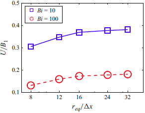
Figure 20. Convergence characteristics of the swimming speed with grid resolution $r_{eq}/\Delta x$
for an ellipsoidal squirmer with
$r_{eq}/\Delta x$
for an ellipsoidal squirmer with $a_r=2$
in a Bingham fluid.
$a_r=2$
in a Bingham fluid.


 Open access