Flow-induced oscillations of an S-shaped buckled flexible filament

Abstract

The flow-induced oscillation of an S-shaped buckled flexible filament was explored using the penalty immersed boundary method. As the length and bending rigidity of the filament were varied, three distinct modes emerged: the equilibrium mode, streamwise oscillation (SO) mode and transverse oscillation (TO) mode. A transition region between the SO and TO modes was identified. Notably, the filament exhibited a 3P wake pattern under SO and a 2S wake pattern under TO. The former was induced by fluid–elastic instability, while the latter was attributed to vortex-induced oscillation. The interaction between the filament's motion and vortex shedding was examined for both modes. To elucidate the disparity between the TO of the S-shaped buckled filament and snap-through oscillation (STO), a ball-on-a-hill analogy was introduced. The performance of energy harvesting was evaluated using metrics including the elastic energy and power coefficient. The TO mode was found to show significantly higher energy harvesting performance than the SO and STO modes. The majority of the strain energy was concentrated at the upper and lower midpoints of the filament.

1. Introduction

Amid growing concerns over environmental damage caused by conventional fossil fuels, there is a pressing need to explore cleaner energy sources as alternatives. Flexible structures embedded with piezoelectric materials, which when placed in a flowing fluid convert the kinetic energy of the flow into electronic energy, have garnered considerable attention (Betts et al. 2012; Harne & Wang 2013). These structures provide a sustainable solution for generating energy while reducing carbon emissions. Buckled filaments, which are clamped on both sides and store significant elastic energy in their initial state, offer greater potential for energy harvesting than single-filaments clamped on only one side (Kim et al. 2021a; Mao, Liu & Sung 2023). Notably, an S-shaped buckled filament subjected to a uniform flow undergoes substantial deflection and can sustain oscillations, making it well-suited to applications in which energy is harnessed from flow-induced oscillations. Understanding the flow-induced oscillation of an S-shaped buckled flexible filament is desirable for advancing the field of flexible energy harvesting.

Considerable research effort has been dedicated to exploring different flow-induced oscillations of a single-clamped flag (or filament). These flags can be categorized into two types based on their clamping position: conventional flags and inverted flags. A conventional flag is defined as having a clamped leading edge and a free trailing edge. This flag configuration displays two distinct modes, known as stretched-straight and flapping, depending on the filament mass, bending rigidity and length (Zhang et al. 2000; Shelley, Vandenberghe & Zhang 2005; Michelin, Llewellyn Smith & Glover 2008; Shelley & Zhang 2011; Banerjee, Connell & Yue 2015; Cisonni et al. 2017). The transition between these two modes is induced by a constructive interaction between the movement of the filament and the fluid force. The critical velocity required to activate the oscillation mode is relatively high (Michelin & Doaré 2013; Xia, Michelin & Doaré 2015; Yu & Liu 2016); however, the critical velocity can be decreased by placing a bluff body upstream of the filament (Allen & Smits 2001; Manela & Howe 2009; Gilmanov, Le & Sotiropoulos 2015; Furquan & Mittal 2021). The inverted flag, which has a clamped trailing edge and a free leading edge, was introduced by Kim et al. (2013) to reduce the critical velocity. The inverted flag exhibits three modes, the straight, flapping and deflected modes, depending on the bending rigidity of the filament and the flow velocity (Ryu et al. 2015; Park et al. 2016). Flapping of the inverted flag is initiated by periodic vortex shedding from the leading and trailing edges (Sader, Huertas-Cerdeira & Gharib 2016b). The inverted flag exhibits a larger oscillation amplitude with a lower critical velocity, which is beneficial for energy harvesting (Gurugubelli & Jaiman 2015; Tang, Liu & Lu 2015; Sader et al. 2016a; Orrego et al. 2017; Yu, Liu & Chen 2017). The free edge of conventional and inverted flags limits their deflection amplitude, thereby restricting their energy harvesting efficiency.

Compared with filaments clamped at one edge, buckled filaments clamped at both edges can store more energy due to their large initial deflection. Kim et al. (2020) proposed a flow-induced energy harvester based on the snap-through oscillation (STO) of such buckled filaments. The STO is a swift transition from one equilibrium state to another in a system, similar to the rapid closure of a Venus flytrap (Forterre et al. 2005) or the sudden upwards flip of an umbrella in the wind (Gomez, Moulton & Vella 2017), resulting in significant deflection (Kim et al. 2021a; Kim, Kim & Kim 2021b). Mao, Liu & Sung (2023) systematically explored the effects of filament length, bending rigidity and Reynolds number on the snap-through dynamics of buckled filaments using the immersed boundary (IB) method. With variations in these parameters, they observed three distinct modes: the STO mode, streamwise oscillation (SO) mode and equilibrium (E) mode. The buckled filaments exhibit considerably more elastic energy during STO than the single-clamped flags, indicating their potential for energy harvesting. The critical bending rigidity required to activate STO is relatively low, which limits the application of buckled flexible filaments in energy harvesting. To increase the critical rigidity, different edge conditions have been explored. For example, a buckled flexible filament with a simply supported leading edge and a clamped trailing edge exhibits a higher critical bending rigidity than the original configuration (Chen et al. 2023). Additionally, channel wall effects could also increase the critical bending rigidity of STO (Chen et al. 2024). Although these methods can be used to modify the initiation condition of STO, the critical bending rigidity remains lower than that of the corresponding inverted flag, limiting the application of buckled flexible filaments in energy harvesting. Serpentine S-shaped buckled flexible filaments, clamped at both edges in opposing directions, store a high amount of elastic energy and can sustain oscillations within the confines of their clamped boundary conditions (Ham et al. 2024). Numerical simulation offers advantages for parametric and quantitative analyses of fluid–flexible structure interactions. In particular, the IB method has been widely adopted to handle this interaction (Huang, Shin & Sung 2007; Huang & Sung 2010; Huang, Chang & Sung 2011; Ryu et al. 2015; Park, Ryu & Sung 2019). Few numerical studies on flow-induced oscillations of S-shaped buckled filaments have been reported. More importantly, the mechanisms underlying the superior energy harvesting efficiency of these filaments have not yet been fully elucidated and warrant a more detailed investigation.

The objective of the present study is to explore the flow-induced oscillations of an S-shaped buckled flexible filament using the penalty IB method. Specifically, we analyse the influence of bending rigidity ($\gamma $) and filament length ($L$) on the filament's motion. Three distinct modes emerge as we vary $\gamma $ and $L$: the E, SO and transverse oscillation (TO) modes. We discern the transition between the SO mode and the TO mode. The oscillation amplitude and frequency, which are the main parameters relative to energy harvesting efficiency, are examined as $\gamma $ and L vary. To elucidate the mechanism of each mode, we analyse vorticity and pressure contours, while also tracking the temporal evolution of force and energy. Furthermore, we evaluate the energy harvesting performance using the elastic energy and power coefficient as metrics. Finally, we investigate the distribution of energy along the filament to determine the optimal positions for attaching piezoelectric patches.

2. Computational model

2.1. Problem formulation

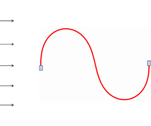
A schematic of the S-shaped buckled flexible filament in a uniform flow is shown in figure 1. The fluid motion is defined on a fixed Cartesian grid, with the computational domain being $- 10{L_0} \le x \le 22{L_0}$ and $- 8{L_0} \le y \le 8{L_0}$, where x and y represent the streamwise and transverse directions, respectively. Dirichlet boundary conditions ($u = {U_0}$, $v = 0$) are applied at the inlet and at the top and bottom boundaries, while a Neumann-type boundary condition ($\partial \boldsymbol{u}/\partial x = 0$) is imposed at the outlet. The fluid motion is initialized as $u = {U_0}$ and $v = 0$. The filament's motion is defined on a moving Lagrangian grid in a curvilinear coordinate system ($s$), where s is the arclength of the filament. Here ${L_0}$ and L denote the distance between the two clamped edges and the total length of the filament, respectively. The leading and trailing edges of the filament are fixed at ($- 0.5,0$) and ($0.5,0$), respectively. The blue rectangles in figure 1 represent clamped boundary conditions at the filament edges. Here $({x_{um}},{y_{um}})$ and $({x_{lm}},{y_{lm}})$ indicate the positions of the upper and lower midpoints of the S-shape, respectively.

Figure 1. Schematic of the S-shaped buckled flexible filament in a uniform flow.

Incompressible viscous fluid flow is governed by the Navier–Stokes equations and the continuity equation, which are represented in non-dimensional form as

(2.1)\begin{gather}\frac{{\partial \boldsymbol{u}}}{{\partial t}} + \boldsymbol{u}\boldsymbol{\cdot }\boldsymbol{\nabla }\boldsymbol{u} =- \boldsymbol{\nabla }p + \frac{1}{{Re}}{\nabla ^2}\boldsymbol{u} + \boldsymbol{f},\end{gather}

(2.2)\begin{gather}\boldsymbol{\nabla }\boldsymbol{\cdot }\boldsymbol{u} = 0,\end{gather}

where $\boldsymbol{u} = (u,v)$ represents the velocity vector of the fluid, p is the pressure and $\boldsymbol{f} = (\,{f_x},{f_y})$ is the momentum forcing used to enforce the no-slip condition along the IB. The Reynolds number is defined as $Re = {\rho _0}{U_0}{L_0}/\mu $, where ${\rho _0}$ and $\mu $ are the fluid density and the dynamic viscosity, respectively. Equations (2.1) and (2.2) are non-dimensionalized using the following characteristic scales: ${L_0}$ for length, ${U_0}$ for velocity, ${L_0}/{U_0}$ for time, ${\rho _0}U_0^2$ for pressure and ${\rho _0}U_0^2/{L_0}$ for the feedback momentum forcing $\boldsymbol{f}$. For convenience, the dimensionless quantities are written in the same form as their dimensional counterparts.

The motion of the filament is governed by the dimensionless nonlinear structure equation and the inextensibility condition,

(2.3)\begin{gather}\frac{{{\partial ^2}\boldsymbol{X}}}{{\partial {t^2}}} = \frac{\partial }{{\partial s}}\left( {T\frac{{\partial \boldsymbol{X}}}{{\partial s}}} \right) - \gamma \frac{\partial }{{\partial s}}\left( {\frac{{\partial K}}{{\partial s}}\boldsymbol{n}} \right) - {\boldsymbol{F}_f},\end{gather}

(2.4)\begin{gather}\frac{{\partial \boldsymbol{X}}}{{\partial s}}\boldsymbol{\cdot }\frac{{\partial \boldsymbol{X}}}{{\partial s}} = 1,\end{gather}

where $\boldsymbol{X} = (X(s,t),\;Y(s,t))$ denotes the displacement vector of the filament, s is the arclength in the range (0, L), T denotes the tension coefficient along the filament, $\gamma $ is the bending rigidity of the filament and ${\boldsymbol{F}_f}$ is the Lagrangian momentum forcing exerted by the surrounding fluid on the filament. Equations (2.3) and (2.4) are non-dimensionalized by the following characteristic scales: ${L_0}$ for length, ${L_0}/{U_0}$ for time, ${\rho _1}U_0^2$ for the tension coefficient T, ${\rho _1}U_0^2L_0^2$ for the bending rigidity $\gamma $ and ${\rho _1}U_0^2/{L_0}$ for the Lagrangian forcing ${\boldsymbol{F}_f}$, where ${\rho _1}$ denotes the density difference between the filament and the surrounding fluid. Given that the filament's cross-sectional length is negligible, ${\rho _1}$ is treated as the filament's density. Here ${\boldsymbol{F}_s} = (\partial /\partial s)T(\partial \boldsymbol{X}/\partial s) - \gamma (\partial /\partial s)(\partial K/\partial s)\boldsymbol{n}$ is the elastic force of the filament. In the present study, $\gamma $ is assumed to be constant, while T is assumed to be a function of s and t, determined by the constraint of inextensibility. A Poisson equation is employed to solve for the value of T (Huang, Shin & Sung 2007). Clamped boundary conditions are imposed at the two fixed edges of the filament, which are

(2.5)\begin{equation}\frac{{\partial \boldsymbol{X}}}{{\partial s}} = (0,1)\quad \textrm{at}\;s = 0,L.\end{equation}

The penalty IB method is utilized to resolve the interaction between the filament and the fluid. A massive boundary and a massless boundary connected by a stiff spring are introduced to model the interaction, and ${\boldsymbol{F}_f}$ is calculated using the following equation (Goldstein, Handler & Sirovich 1993):

(2.6)\begin{equation}{\boldsymbol{F}_f} = \alpha \int_0^t {({\boldsymbol{U}_{ib}} - \boldsymbol{U})\,\textrm{d}t^{\prime}} + \beta ({\boldsymbol{U}_{ib}} - \boldsymbol{U}),\end{equation}

where $\alpha =- 3 \times {10^6}$ and $\beta =- 100$ are large negative constants, chosen to enforce the no-slip condition (Huang et al. 2007; Shin, Huang & Sung 2008). Here, ${\boldsymbol{U}_{ib}}$ denotes the velocity of the massless boundary obtained by interpolation at the IB, and $\boldsymbol{U}$ is the velocity of the massive boundary obtained by $\boldsymbol{U} = \textrm{d}\kern0.7pt \boldsymbol{X}/\textrm{d}t$. The transformation between Euler and Lagrangian variables can be realized using the Dirac delta function; ${\boldsymbol{U}_{ib}}$ and $\boldsymbol{f}$ can be obtained using the following equations:

(2.7)\begin{gather}{\boldsymbol{U}_{ib}}(s,t) = \int_\varOmega {\boldsymbol{u}(x,t)\; \delta (\boldsymbol{X}(s,t) - x)\,\textrm{d}\kern0.06em x} ,\end{gather}

(2.8)\begin{gather}\boldsymbol{f}(x,t) = \rho \int_\varGamma {{\boldsymbol{F}_f}(s,t)\delta (x - \boldsymbol{X}(s,t))\,\textrm{d}s} ,\end{gather}

where the density ratio ($\rho $) is derived from the non-dimensionalization process ($\rho = {\rho _1}/{\rho _0}{L_0} = 1$). In this context, ${\rho _1}$ refers to the line density, whereas ${\rho _0}$ represents the area density. The elastic strain energy ${E_s}(t)$, a parameter that can be used to estimate the energy harvesting performance, is defined as

(2.9)\begin{equation}{E_s}(t) = \int_\varGamma {0.5\gamma {K^2}(s,t)\,\textrm{d}s} ,\end{equation}

where K is the curvature.

To estimate the electricity generated by piezoelectric patches on the surface of the oscillating filament, we consider piezo-structure coupling. The filament is assumed to be equipped with infinitesimal piezoelectric patches on both sides, with segmentation lengths much smaller than L. An output electric circuit is coupled to the deflection of the filament by the piezoelectric effect, where stretching and compression of the patches induce charge transfer between each patch's electrodes. An electric voltage applied to the electrodes results in additional internal torque on the piezoelectric patch and the filament (Doaré & Michelin 2011). Each patch's local electric state is characterized by the electric voltage between the positive electrodes of each patch, denoted by $V(s,t)$, and the charge transfer $Q(s,t)$ along the filament axis; both parameters are continuous functions of s and t (Michelin & Doaré 2013). The piezoelectric coupling effect is modelled by the following equations:

(2.10)\begin{gather}Q(s,t) = cV + \chi K,\end{gather}

(2.11)\begin{gather}M(s,t) =- \gamma K + \chi V,\end{gather}

where $M(s,t)$ represents the torque of the filament, $\boldsymbol{n}$ is the unit normal vector and c and $\chi $ are the lineic capacitance and piezoelectric coupling coefficient, respectively, which are related to the material and geometric properties of the patch pair (Doaré & Michelin 2011). The positive electrodes are connected to a purely resistive circuit with lineic conductivity, as described by the equation

(2.12)\begin{equation}\frac{{\partial Q}}{{\partial t}}(s,t) =- \varsigma V,\end{equation}

where $\varsigma $ is the linear conductivity coefficient between the piezoelectric patches on the upper and lower surfaces of the filament. Considering the piezoelectric effect, the equivalent bending rigidity can be expressed as

(2.13)\begin{equation}{\gamma _E} = \frac{{\partial M}}{{\partial s}} =- \gamma \frac{{\partial K}}{{\partial s}} + \chi \frac{{\partial V}}{{\partial s}}.\end{equation}

After combining equations (2.10)–(2.13), the nonlinear structure equation with the piezoelectric effect and the electrical equation can be expressed as follows:

(2.14)\begin{gather}\frac{{{\partial ^2}\boldsymbol{X}}}{{\partial {t^2}}} = \frac{\partial }{{\partial s}}\left( {T\frac{{\partial \boldsymbol{X}}}{{\partial s}}} \right) - \gamma \frac{\partial }{{\partial s}}\left( {\frac{{\partial K}}{{\partial s}}\boldsymbol{n}} \right) + {\alpha _e}\sqrt \gamma \frac{\partial }{{\partial s}}\left( {\frac{{\partial V}}{{\partial s}}\boldsymbol{n}} \right) - {\boldsymbol{F}_f},\end{gather}

(2.15)\begin{gather}{\beta _e}\frac{{\partial V}}{{\partial t}} =- V - {\alpha _\textrm{e}}{\beta _e}\sqrt \gamma \frac{{\partial K}}{{\partial t}},\end{gather}

where ${\alpha _e} = \chi /\sqrt {c{\gamma _L}} $ and ${\beta _e} = cU/(\varsigma L)$ are the coupling coefficient and the tuning coefficient of the electrical system, respectively (Shoele & Mittal 2016). Here, ${\gamma _L}$ represents the dimensional bending rigidity. The voltage and charge density are non-dimensionalized by $U\sqrt {\rho L/c} $ and $U\sqrt {\rho Lc} $, respectively. In the present study, we do not specifically investigate the effects of ${\alpha _e}$ and ${\beta _e}$, which are kept constant at 0.1 and 0.1, respectively, without disturbing the filament motion.

The harvested energy is equal to the instantaneous power dissipated in the piezo patches (Michelin & Doaré 2013; Shoele & Mittal 2016). A power coefficient normalized by the kinetic energy flux of the fluid ($\rho {U^3}L$) is used to estimate the energy harvesting performance, defined as

(2.16)\begin{equation}{c_p} = \frac{P}{{\rho {U^3}L}} = \frac{1}{{{\beta _e}}}\int_0^1 {{V^2}\,\textrm{d}s} .\end{equation}

Based on the dimensional analysis by Shoele & Mittal (2016), ${\bar{c}_p}\sim \gamma {f^2}{K^2}$, where f represents the frequency of the filament.

The fractional step method on a staggered Cartesian grid is adopted to solve the Navier–Stokes equations (Kim, Baek & Sung 2002). A direct numerical method developed by Huang, Shin & Sung (2007) is employed to calculate the filament motion. Details regarding the discretization of the governing equations and numerical method can be found in the works of Kim, Sung & Hyun (1992) and Kim, Baek & Sung (2002).

2.2. Validation

Table 1 shows the results of the domain test for $L/{L_0} = 2$, $\gamma = 0.01$ and $Re = 100$ including the averaged drag coefficient ${\bar{C}_D}$, root mean square (r.m.s.) of the lift coefficient ${C_{L\;rms}}$ and the Strouhal number $St$ ($\,{f_v}{L_0}/{U_0}$), along with the corresponding relative error $\varepsilon $. Here, ${f_v}$ represents the shedding frequency of vortices from the filament. The results for the $32 \times 16$ domain are consistent with those for the $32 \times 24$ and $64 \times 16$ domains. Thus, a domain size of $32 \times 16$ was chosen because it allows simulation of the system for a greater number of time steps, thus enhancing the accuracy of the results. To assess the impact of grid resolution and time step on the simulation results, convergence studies were conducted for different grid resolutions and time steps. Figure 2 shows the time evolution of the transverse displacement of the upper midpoint of the filament. The results obtained with $\Delta x = 1/64$ and $\Delta t = 4 \times {10^{ - 4}}$ match well with those for $\Delta x = 1/128$ and $\Delta t = 2 \times {10^{ - 4}}$, with maximum relative errors in ${y_{um}}$ of 0.015 and 0.008, respectively. The result does not converge for $\Delta x > 1/32$. A grid resolution of $1/64$ and a time step of $4 \times {10^{ - 4}}$ were chosen to ensure sufficiently high accuracy of the simulation. The maximum Courant number was approximately 0.04 in the simulation. The grid was uniform in the $x$-direction but stretched in the $y$-direction. Specifically, within the range $- Y/4 \le y \le Y/4$, the grid size was $\Delta y = \Delta x$, and outside of this range the grid size was $\Delta y = 2\Delta x$. The grid size of the filament matched that of the fluid domain.

Table 1. Domain test, including the averaged drag coefficient ${\bar{C}_D}$, r.m.s. of the lift coefficient ${C_{L\;rms}}$, the Strouhal number $St$ and the relative errors $\varepsilon $ to $32 \times 24$ (domain height test in part I) and $64 \times 16$ (domain length test in part II) for $L/{L_0} = 2$, $\gamma = 0.01$ and $Re = 100$.

Figure 2. Time evolution of the transverse displacement of the upper midpoint of the filament (${y_{um}}$) for different (a) grid resolutions and (b) time steps.

Furthermore, we conducted an experiment in a small open suction wind tunnel (Re = 8500), as shown in figure 3(a). The red line shows the superposition of the instantaneous shapes observed in the experiment, while the solid line represents our simulation results. Despite the higher oscillation frequency in the experiment (50 Hz) compared with the simulation, the close alignment between the experimental and simulated shapes suggests that our solver effectively captures the interaction dynamics of large deformations. Figure 3(b) examines the effect of the aspect ratio $W/L$, where W is the spanwise length, on the oscillation amplitude ${A_y}$. As $W/L$ increases beyond 2, ${A_y}$ converges to a constant value, suggesting that the effect of $W/L$ is negligible. This observation aligns with previous studies on conventional flags (Banerjee, Connell & Yue 2015; Gurugubelli & Jaiman 2019). We believe that our simulation provides an accurate interpretation of the real-world application of energy harvesting where $W/L$ is sufficiently large. Further details on the experimental set-up used to obtain the results shown in figure 3 are available in Lyu, Cai & Liu (2024).

Figure 3. (a) Comparison of the experiment and the present simulation. (b) Oscillation amplitude (${A_y}$) as a function of the aspect ratio ($W/L$).

3. Results and discussion

3.1. Modes of filament motion

Three different modes of the S-shaped buckled flexible filament are detected as $L/{L_0}$ and $\gamma $ vary: the SO mode, TO mode and E mode. Superpositions of the instantaneous shapes of a filament in the SO, TO and E modes are shown in figure 4. At low $\gamma $ values $(L/{L_0} = 2.25)$, the SO mode is predominant, characterized by the filament being too soft to maintain its S-shape under fluid force, resulting in a downwards tilt. The unsteady fluid force induced by vortex shedding and large-amplitude filament motion leads to the SO mode of the filament. As $\gamma $ is increased $(L/{L_0} = 1.75)$, the filament attains sufficient rigidity to maintain its distinctive S-shape, thereby transitioning into the TO mode. This transition is facilitated by the periodic shedding of vortices, which create a recurring transverse fluid force, causing the filament to oscillate transversely. Once $\gamma $ exceeds a critical value, the filament transitions into an equilibrium state without any motion, referred to as the E mode. Figure 4(c) illustrates the E mode under three different $\gamma $ values. As $\gamma $ increases $(L/{L_0} = 1.5)$, the filament can resist the fluid force with less deformation, resulting in a decrease in the tilt to the streamwise direction. When $\gamma $ reaches a relatively high value (e.g. $\gamma = 1$), the filament exhibits a shape similar to its initial shape without flow.

Figure 4. Superposition of the instantaneous shapes of the filament in the (a) SO mode ($L/{L_0} = 2.25$, $\gamma = 0.005$), (b) TO mode ($L/{L_0} = 1.75$, $\gamma = 0.1$) and (c) E mode ($L/{L_0} = 1.5$, $\gamma = 0.005$, 0.02, 1).

Next, we consider the effect of $\gamma $ and $L/{L_0}$ on the mode transitions of the S-shaped buckled flexible filament. Figure 5 shows a mode diagram covering the range of $0.0001 \le \gamma \le 10$ and $1.25 \le L/{L_0} \le 2.25$. The length of the filament significantly influences its motion and the presence of different modes. When $L/{L_0}$ is less than 1.5, the filament remains in the E mode at all $\gamma $ values. This occurs because shorter filaments lack adequate space for deformation, resembling a filament under full tension. Additionally, when $L/{L_0}$ is lower than 1.5, there is no shedding of vortices, indicating the absence of unsteady fluid forces to initiate filament motion. This results in the predominance of the E mode for short filaments. Once $L/{L_0}$ reaches 1.5, the TO mode is observed at $\gamma = 0.1$, accompanied by vortex shedding. Under these conditions, the resonance between the filament structure and shedding vortices initiates the TO mode. As $L/{L_0}$ increases to 2, the filament becomes more flexible, and the critical $\gamma $ required to sustain the TO mode significantly increases. The distribution of modes is determined by the bending rigidity of the filament. The SO mode appears at low $\gamma $ ($0.0001 < \gamma < 0.05$), while the filament shifts to the TO mode as $\gamma $ is increased into the range $0.05 \le \gamma \le 5$. The E mode predominates when $\gamma $ is high and/or $L/{L_0}$ is low.

Figure 5. Diagram showing the dependence of the filament mode on $\gamma $ and $L/{L_0}$. Circle and triangle markers represent the absence and presence of vortex shedding in the wake, respectively ($Re = 100$).

The wake pattern and power spectral density (PSD) of v at $x = 5$ and $y = 0$ are explored for the three different modes, as illustrated in figure 6(a,b), respectively. When the filament is in the SO mode, a 3P wake pattern is observed, indicating the shedding of three pairs of vortices during one SO motion. The details of the vortex shedding process will be discussed later. The PSD of the SO mode exhibits three distinct peaks. The prominent peak ${f_v}$, equal to $3{f_{{y_{um}}}}$, represents the vortex shedding frequency of the 3P wake pattern, where ${f_{{y_{um}}}}$ is the oscillation frequency of the filament. The other two peaks indicate disturbances in the motion of the filament. In the TO mode, the filament exhibits a 2S wake pattern, with two single vortices shed in one TO period. The PSD shows only one peak, with ${f_v} = {f_{{y_{um}}}}$, indicating that the periodic vortex shedding is synchronized with the TO, providing evidence that TO is a vortex-induced oscillation. Similar to the TO mode, the E mode also exhibits a 2S wake pattern and has a PSD with a single peak.

Figure 6. (a) Instantaneous contours of ${\omega _z}$ and (b) PSD of v ($x = 5$, $y = 0$) for the SO mode ($L/{L_0} = 2.25$, $\gamma = 0.005$), TO mode ($L/{L_0} = 2$, $\gamma = 0.1$) and E mode ($L/{L_0} = 1.75$, $\gamma = 1$).

The time histories of the upper midpoint and lower midpoint of the filament, as well as the sequential process of the SO, are examined to elucidate the SO motions of the S-shaped filament. The five times examined, denoted by A, B, C, D and E, correspond to the times at which ${x_{um}}$ and ${y_{um}}$ reach their extreme values. From the time histories in figure 7(a,b), it is clear that the first half ($0 \le s < L/2$) and the second half ($L/2 \le s < L$) of the filament undergo totally different motions. This is due to the filament losing its central symmetry in the SO mode. At time A, ${y_{um}}$ reaches its maximum value and ${x_{um}}$ reaches its minimum value. From A to B, the filament moves upstream due to the elastic force, with minimal change in the values of ${x_{lm}}$ and ${y_{lm}}$ during this interval. After time B, the fluid force pushes the filament downstream. From B to C, ${x_{lm}}$ decreases and ${y_{lm}}$ increases, while ${x_{um}}$ and ${y_{um}}$ remain almost constant. From C to D, ${y_{um}}$ decreases and ${y_{lm}}$ increases, indicating that the first half of the filament is moving downwards and the second half is moving upwards. At time D, ${x_{um}}$ reaches a maximum value and ${y_{um}}$ reaches a minimum value. From D to E, ${x_{um}}$ decreases and ${y_{um}}$ increases, indicating that the first half of the filament is moving upstream while the second half is moving downwards, with ${y_{lm}}$ decreasing. At time E, one period comes to an end, and the filament starts a new SO motion. The motion of the SO mode is not regular, exhibiting markedly different behaviours in the first and second halves of the filament. This complexity arises from the intricate interaction between the filament and the surrounding fluid, where the motion of the filament influences vortex shedding and, in turn, the shed vortices impact the motion of the filament.

Figure 7. Time histories of the (a) upper midpoint (${x_{um}}$, ${y_{um}}$) and (b) lower midpoint (${x_{lm}}$, ${y_{lm}}$) in the SO mode. (c) The sequential process of the SO mode ($L/{L_0} = 2.25$, $\gamma = 0.005$).

The motion of the TO mode is more regular than that observed for the SO mode, which is beneficial for providing a steady voltage output. Figure 8 illustrates the time histories of the upper midpoint and lower midpoint, accompanied by the sequential process of the TO mode. At times A, C and E, both ${x_{um}}$ and ${y_{um}}$ reach their extreme values, signifying significant positional shifts. Conversely, times B and D correspond to instances when the filament midpoint ($s = L/2$) intersects the $y = 0$ plane. At time A, both ${x_{um}}$ and ${x_{lm}}$ reach their maximum values, while ${y_{um}}$ and ${y_{lm}}$ reach their minimum values. This configuration suggests that at this time the filament has attained its most downstream and downwards position. From A to B, the filament moves upwards and upstream. At time B, the filament assumes an S-shape resembling its initial configuration. Progressing from B to C, the filament undergoes continued upwards and upstream motion, ultimately reaching its extreme upstream and upwards position at time C. Subsequently, from C to E, the filament initiates a downwards motion, mirroring its earlier upwards trajectory. Following time E, a new period of the TO mode ensues. Notably, the motion of the lower midpoint mirrors that of the upper midpoint. However, the amplitude of ${y_{lm}}$ is slightly larger than ${y_{um}}$ due to the asymmetry of the flow field along the $y = 0$ axis. The first half of the filament experiences a greater fluid force, which suppresses its amplitude.

Figure 8. Time histories of the (a) upper midpoint (${x_{um}}$, ${y_{um}}$) and (b) lower midpoint (${x_{lm}}$, ${y_{lm}}$) in the TO mode. (c) The sequential process of the TO mode ($L/{L_0} = 2$, $\gamma = 0.1$).

3.2. Effects of bending rigidity

In this section, we explore the effects of bending rigidity on the S-shaped buckled filament. The frequencies of filament oscillation and vortex shedding, along with the oscillation amplitude, are utilized to identify the modes of the filaments, as shown in figure 9(a,b). Figure 9(c) depicts the average shape of the filament at various $\gamma $ values corresponding to different modes. The symbol ‘T’ represents the transition region between the SO and TO modes. In the SO mode ($0.0001 \le \gamma < 0.005$), the oscillation frequency of the filament differs from the vortex shedding frequency, whereas these two frequencies are similar in the TO mode. This discrepancy is one of the main differences between the SO and TO modes. The difference between ${f_v}$ and ${f_{{y_{um}}}}$ in the SO mode also suggests that this mode cannot be classified as a form of vortex-induced vibration. Furthermore, filaments in the SO mode have lower oscillation amplitudes in the x and y directions compared with those in the TO mode.

Figure 9. (a) Frequencies of filament oscillation ($\,{f_{{y_{um}}}}$) and vortex shedding ($\,{f_v}$) as a function of $\gamma $. (b) Oscillation amplitude in the x (${A_x}$) and y (${A_y}$) directions as a function of $\gamma $. (c) Mean filament shape at different $\gamma $ values for the three modes ($L/{L_0} = \; 2$).

In figure 9, increasing $\gamma $ causes the filament to tilt upstream, suggesting that it becomes more robust in resisting fluid forces. In the SO mode, the filament moves downstream, driven by a combination of the positive fluid force in the x-direction and the clockwise moment. Once $\gamma $ surpasses 0.005, the filament enters a transitional (T) region in which both SO and TO motions are observed. At $\gamma = 0.005$, the filament remains almost static, with ${A_x}$ and ${A_y}$ approaching zero. This static state arises from a delicate equilibrium between fluid and elastic forces. Similar observations were made for filaments with $L/{L_0}$ ratios of 1.75 and 2.25. When $\gamma $ is further increased, the mean position of the filament keeps tilting upstream and the oscillation amplitude increases, indicating that the filament motion is approaching the TO mode. The shift to the TO mode is complete after $\gamma $ surpasses 0.05. At $\gamma = 0.1$, the oscillation amplitudes peak as the vortex shedding frequency approaches the resonance frequency of the filament (Argentina & Mahadevan 2005). Similar resonance phenomena are also observed around $\gamma = 0.1$ in filaments with $L/{L_0}$ ratios of 1.75 and 2.25. As $\gamma $ is increased beyond 0.1, the oscillation amplitude decreases and the mean shape gradually returns to that of the initial configuration of the filament. In the TO mode, a lock-in phenomenon is evident near the resonance frequency depicted in figure 9(a), implying that TO is likely a result of vortex-induced vibration. Once $\gamma $ surpasses 5, the filament becomes sufficiently robust to withstand the fluid forces, leading to the emergence of the E mode.

To investigate the interaction between filament motion and vortex dynamics during oscillation, we conducted a detailed analysis of the time histories of ${x_{um}}$, ${y_{um}}$, $\boldsymbol{F}$ and E, and examined instantaneous contours of ${\omega _z}$ and p. Initially, we focus on the interaction in the SO mode. We specifically examine four distinct time steps denoted by A, B, C and D, as illustrated in figure 10. Here, ${F_{fx}}$ and ${F_{fy}}$ represent the $x$-direction and $y$-direction fluid forces, respectively, while ${F_{sx}}$ and ${F_{sy}}$ denote the $x$-direction and $y$-direction elastic forces, respectively. The total energy of the filament ($E$) is composed of the elastic energy (${E_s}$) and kinetic energy (${E_k}$). At time A, ${y_{um}}$ reaches its maximum value, coinciding with the shedding of a pair of vortices ${V_{p1}}$ from the filament. This shedding creates a low-pressure area on top of the filament, resulting in the maximum value of ${F_{fy}}$. Both ${E_k}$ and ${E_s}$ are relatively low at this time. As the system evolves from A to B, the filament moves downstream under the influence of a positive ${F_{fx}}$. Concurrently, a pair of vortices, denoted by ${V_{p2}}$, detach from the filament due to the SO motion, inducing a negative ${F_{fy}}$ that pushes the filament downwards at time B. Notably, ${E_s}$ reaches its minimum value at this point, indicating minimal deflection. The downstream and downwards motion of the filament continues from B to C, accompanied by increases in ${F_{sx}}$, ${F_{sy}}$ and ${E_s}$. At time C, ${y_{um}}$ reaches its minimum value with the shedding of ${V_{p3}}$. At this time, ${E_s}$ attains its maximum value, signifying that the filament has sufficient potential to resist fluid forces. Finally, at time D, ${E_k}$ reaches its maximum value, while ${E_s}$ reaches its local minimum value, suggesting a conversion of part of ${E_s}$ to ${E_k}$, resulting in the filament moving upwards. Subsequent to time D, the filament moves upstream and upwards under the influence of elastic forces, leading to a significant reduction in elastic energy. In summary, the SO mode is induced by sustained $x$-direction fluid forces, boundary conditions and vortex shedding. A high-pressure area is maintained at the front part of the filament during the SO motion, influenced by the main stream. This high-pressure area compels the filament to move downstream. The filament experiences elastic forces due to the boundary conditions, striving to overcome fluid forces and return to its equilibrium position. The shedding vortices disrupt the balance between the fluid and elastic forces, contributing to the instability of the filament. Under the influence of these factors, the SO mode is sustained.

Figure 10. (a) Time histories of ${x_{um}}$, ${y_{um}}$, $\boldsymbol{F}$ and E. Instantaneous contours of (b) ${\omega _z}$ and (c) p at times A, B, C and D for $L/{L_0} = 2$ and $\gamma = 0.002$ in the SO mode.

We now shift our focus to the interaction between filament motion and vortex dynamics in the TO mode. Time steps A and C denote when ${x_{um}}$ and ${y_{um}}$ reach their extreme values, while times B and D correspond to when the filament midpoint ($s = L/2$) crosses $y = 0$. Notably, ${F_{fx}}$ and ${F_{sx}}$ are lower than ${F_{fy}}$ and ${F_{sy}}$, respectively, indicating that the $y$-direction force is a major factor in the TO mode. At time A, ${y_{um}}$ reaches its minimum value and ${x_{um}}$ reaches its maximum value, accompanied by the shedding of a positive ${V_s}$ from the filament. This behaviour is facilitated by the development of a high-pressure region at the rear end of the filament, which minimizes ${F_{fy}}$. Because the filament is at an extreme position at time A, all kinetic energy converts to elastic energy, leading to a maximum value of ${F_{sy}}$. Transitioning from A to B, the elastic forces overcome the resistance of the fluid forces, initiating an upwards motion. At time B, the filament returns to an equilibrium state, with almost all elastic energy converting to kinetic energy, resulting in a low ${E_s}$ and a high ${E_k}$. ${F_{sy}}$ is nearly zero due to the low ${E_s}$. Progressing from B to C, the filament continues moving under the influence of inertia, with ${F_{sy}}$ decreasing and ${F_{fy}}$ increasing during this period. At time C, the filament reaches another extreme position, where ${y_{um}}$ reaches its maximum value and ${x_{um}}$ reaches its minimum value, accompanied by the shedding of a negative ${V_s}$ from the filament. Similar to what is observed at time A, a high-pressure area forms below the front part of the filament, resulting in a maximum ${F_{fy}}$. Once again, all ${E_k}$ converts to ${E_s}$, creating conditions that drive the filament into a downwards motion. Notably, the value of ${E_s}$ at time C is higher than that at time A because of the influence of the asymmetric fluid field along the $y = 0$ axis. This asymmetric fluid field also contributes to the asymmetry of the force and filament motion. From C to D, the filament moves downwards under the influence of ${F_{sy}}$. At time D, the filament returns to its equilibrium position, with all ${E_s}$ being converted to ${E_k}$. After time D, the filament moves towards the lower extreme position under the action of inertia, and one TO period comes to an end.

The behaviour of the S-shaped filament in the TO mode shares many similarities with a spring–mass system, such as the conversion of elastic energy and kinetic energy, as well as the increase in elastic force as the system moves away from its equilibrium position. This latter characteristic arises from the clamping of the two edges of the S-shaped filament in the equilibrium position. Specifically, if the filament moves upwards or downwards, the clamped trailing or leading edge imposes a force driving the filament towards its equilibrium position. At low $\gamma $, the S-shape breaks under the positive $x$-direction fluid force, and the filament cannot return to its equilibrium position, leading to the SO mode. As $\gamma $ is increased further, the filament becomes sufficiently robust to sustain the TO mode while adhering to the limitations of its clamped boundary conditions, ensuring that the deflection from equilibrium remains within acceptable parameters. The shedding vortices provide a periodic fluid force, similar to applying a periodic external force to a spring–mass system, thus leading to the TO mode, which induces vortex-induced oscillation.

3.3. Effects of filament length

Filament length is a critical parameter that determines the shape of the filament, thereby influencing its motion. In this section, we explore the effects of $L/{L_0}$ on the motion of an S-shaped buckled filament. Building upon the analysis in § 3.2, where the TO mode exhibited more regular motion and higher oscillation amplitude, indicating greater potential for energy harvesting, we fix $\gamma $ at 0.1 to focus on the effects of $L/{L_0}$ on the S-shaped buckled filament. Figure 12 shows the oscillation frequency and oscillation amplitude as functions of $L/{L_0}$. When $L/{L_0}$ is less than 1.5, the filament is too short to deflect under the constraints of the clamped edges, leading to the E mode. Additionally, the flatter profile of a shorter S-shaped filament prevents fluid separation, inhibiting vortex shedding and consequently eliminating the occurrence of flow-induced oscillations. Once $L/{L_0}$ exceeds 1.5, the filament shifts to the TO mode. As $L/{L_0}$ increases, ${f_{{y_{um}}}}$ decreases due to the decrease in shedding frequency. Conversely, both ${A_x}$ and ${A_y}$ increase with increasing $L/{L_0}$. This phenomenon is intuitive, as longer filaments are more prone to moving.

To examine the interaction between the filament and the shed vortices, instantaneous contours of ${\omega _z}$ and time histories of the fluid force are calculated for different filament lengths, as shown in figure 13. At ${L_0}/L = 1.4$, the shear layers formed at the top of the front part of the filament and bottom of the rear part of the filament remain steady, leading to constant fluid forces and the E mode. As ${L_0}/L$ increases to 1.5, the shear layers become unstable and begin to separate from the filament, giving rise to vortex shedding. The shedding of these vortices generates a periodic fluid force, leading to the periodic TO motion of the filament. On further increase of ${L_0}/L$ to 1.5, the fluid force becomes more complex, indicating its coupling with the motion of the filament. This coupling may result in positive feedback, where higher fluid force leads to a higher oscillation amplitude, and vice versa, making it easier for the S-shaped filament to initiate and sustain the TO mode, as illustrated in figure 11.

Figure 11. (a) Time histories of ${x_{um}}$, ${y_{um}}$, $\boldsymbol{F}$ and E. Instantaneous contours of (b) ${\omega _z}$ and (c) p at times A, B, C and D for $L/{L_0} = 2$ and $\gamma = 0.1$ in the TO mode.

Figure 12. (a) Oscillation frequency and (b) oscillation amplitude as a function of $L/{L_0}$ ($\gamma = 0.1$).

Figure 13. (a) Instantaneous contours of ${\omega _z}$ and (b) time histories of fluid force for ${L_0}/L = 1.4$, 1.5, 1.75 at $\gamma = 0.1$.

3.4. Energy harvesting performance.

Finally, we assess the energy harvesting performance of the S-shaped buckled filament by considering the elastic energy and power coefficient, and compare the results with those obtained for the conventional buckled filament undergoing STO (Mao et al. 2023). Due to the energy stored in the initial shape of the filament, we adopt the available time-averaged elastic energy (${\bar{E}^{\prime}_s} = {\bar{E}_s} - {\bar{E}_{s\;min}}$) and power coefficient (${\bar{c}^{\prime}_p} = {\bar{c}_p} - {\bar{c}_{p\;min}}$) to estimate the harvested energy. Figure 14 shows plots of ${\bar{E}^{\prime}_s}$ and ${\bar{c}^{\prime}_p}$ against $\gamma $ for both the S-shaped and the snap-through configurations with $L/{L_0} = 2$. As $\gamma $ increases, three peaks are observed for the S-shaped configuration (figure 14a), consistent with the oscillation amplitude curve in figure 9(b). The SO mode of the S-shaped filament exhibits two significant peaks in ${\bar{E}^{\prime}_s}$, at $\gamma $ values of approximately 0.002 and 0.01. Filaments with $\gamma < 0.005$ show low elastic energy due to the system being in a T region and nearly static. The filaments demonstrate higher ${\bar{E}^{\prime}_s}$ in the TO mode, with a prominent peak at $\gamma = 0.1$ caused by resonance between the filament and shedding vortices. After surpassing $\gamma = 0.1$, ${\bar{E}^{\prime}_s}$ decreases with increasing $\gamma $. For the conventional buckled filament undergoing STO, ${\bar{E}^{\prime}_s}$ increases as $\gamma $ increases before reaching the critical $\gamma $. After surpassing the critical $\gamma $, the buckled filament shifts to the SO mode, resulting in a sudden decrease in ${\bar{E}^{\prime}_s}$. As $\gamma $ continues to rise, the filament shifts to the E mode, and ${\bar{E}^{\prime}_s}$ steadily diminishes until reaching 0. Importantly, in the range of $0 < \gamma < 0.012$, the STO configuration has a higher ${\bar{E}^{\prime}_s}$ than the S-shaped filament. This discrepancy arises from the greater deflection experienced during the snap-through process. Figure 14(b) shows plots of ${\bar{c}^{\prime}_p}$ as a function of $\gamma $ for both the S-shaped and the STO configurations. For the S-shaped filament, ${\bar{c}^{\prime}_p}$ remains almost negligible for $\gamma < 0.01$. This can be attributed to the fact that ${c_p}$ is a function of $\gamma $ and K, with higher $\gamma $ values leading to increases in ${c_p}$. Consequently, the S-shaped filament in the TO mode demonstrates a significantly higher ${\bar{c}^{\prime}_p}$ than the SO mode. The peak ${\bar{c}^{\prime}_p}$ occurs at $\gamma = 0.5$, which differs from the peak in ${\bar{E}^{\prime}_s}$ due to the effect of $\gamma $. The buckled filament exhibits a higher ${\bar{c}^{\prime}_p}$ under low $\gamma $ due to the large deflection in the STO motion. In contrast, the TO mode exhibits a higher ${\bar{c}^{\prime}_p}$ due to its higher critical bending rigidity and oscillation frequency, making it a more promising candidate for practical energy harvesting applications.

Figure 14. Plots of (a) ${\bar{E}^{\prime}_s}\; $and (b) ${\bar{c}^{\prime}_p}$ as functions of $\gamma $ for the S-shaped filament and conventional buckled filament undergoing STO ($L/{L_0} = 2$).

Figure 15. Plots of (a) ${\bar{E}^{\prime}_s}\; $and (b) ${\bar{c}^{\prime}_p}$ as functions of $L/{L_0}$ ($\gamma = 0.1$).

Next, we examine the energy harvesting performance under different values of $L/{L_0}$ (figure 15). The curves for ${\bar{E}^{\prime}_s}$ and ${\bar{c}^{\prime}_p}$ exhibit a shape similar to that observed in the plot of oscillation amplitude as a function of $L/{L_0}$ at $\gamma = 0.1$ in figure 12(b), as $\gamma $ is fixed at 0.1 and ${c_p}$ is based only on K and ${f_{{y_m}}}$. At low $L/{L_0}$, where the system is in the E mode, the values of ${\bar{E}^{\prime}_s}$ and ${\bar{c}^{\prime}_p}$ are almost 0. As $L/{L_0}$ increases to 1.5, the filament shifts to the TO mode, leading to increases in both ${\bar{E}^{\prime}_s}$ and ${\bar{c}^{\prime}_p}$ with increasing $L/{L_0}$. A sudden increase in ${\bar{E}^{\prime}_s}$ and ${\bar{c}^{\prime}_p}$ around $L/{L_0} = 2$ is caused by the resonance of the filament under shedding vortices. Beyond $L/{L_0} = 2$, ${\bar{E}^{\prime}_s}$ continues to rise, while ${\bar{c}^{\prime}_p}$ decreases at $L/{L_0} = 2.3$ due to a reduction in frequency, as indicated in figure 12(a). Filaments with a length around $L/{L_0} = 2$ exhibit a broader range of TO mode and a higher ${\bar{c}^{\prime}_p}$, making them more suitable for energy harvesting applications.

Figure 16. (a) Time-averaged local elastic strain energy $\langle {E_s}\rangle $ and (b) voltage $\langle V\rangle $ of the filament as a function of $s/L$ for $L/{L_0} = 2$.

Figure 16 shows the time-averaged local strain energy $\langle {E_s}\rangle = (1/T)\int_0^T {0.5\gamma K\,\textrm{d}t} $ and voltage $\langle V\rangle = (1/T)\int_0^T {V\,\textrm{d}t}$ along the filament for different values of $\gamma $. Filaments operating in the TO mode ($\gamma = 0.1$, 0.2) exhibit higher $\langle {E_s}\rangle $ and $\langle V\rangle $ than those operating in the SO mode ($\gamma = 0.02$). As $\gamma $ increases, both $\langle {E_s}\rangle $ and $\langle V\rangle $ increase accordingly, as they are functions of $\gamma $. More elastic energy is concentrated at $s/L = 0.25$ and $s/L = 0.75$, corresponding to the upper midpoint and lower midpoint of the filament, indicating that significant deflection occurs near these parts during TO motion. This large deflection also contributes to a higher $\langle V\rangle $ around $s/L = 0.25$ and $s/L = 0.75$. Based on the above analysis, piezoelectric materials should be attached to the last half of the filament to enhance efficiency.

4. Conclusions

In this study, we investigated the flow-induced oscillation of an S-shaped buckled flexible filament, using the penalty IB method. We systematically analysed the effects of varying $L/{L_0}$ and $\gamma $ on the filament's motion and energy harvesting performance. Three distinct modes were identified as $L/{L_0}$ and $\gamma $ were varied, designated as the SO mode, TO mode and E mode. The filament persisted in the E mode when $L/{L_0} \le 1.4$. Upon exceeding this threshold, the SO mode predominated at low $\gamma $ and the TO mode at high $\gamma $. We explored the wake patterns and the corresponding PSDs of the different modes to elucidate the interplay between filament motion and vortex shedding. The SO mode was induced by fluid–elastic instability due to the interaction between unsteady elastic forces and shedding vortices, whereas the TO mode was considered a vortex-induced oscillation, as indicated by the synchronous presence of TO and vortex shedding, along with matching frequencies between oscillation and vortex shedding. A transition region (T) displaying both SO and TO motions was detected based on oscillation amplitude and frequency. We examined the filament motion and vortex shedding process, accompanied by the time history of force and energy. The SO mode exhibited a 3P wake pattern and irregular motion, attributed to the filament being too soft to sustain its S-shape under the fluid force. In contrast, the filament in the TO mode exhibited a 2S wake pattern, accompanied by regular motion, as it was robust enough to resist deformation of the S-shape, moving near an equilibrium state under vortex shedding. Finally, we estimated the energy harvesting performance of the S-shaped buckled filament by considering the elastic energy and power coefficient, with STO used as a basis for comparison. The TO mode exhibited higher elastic energy than the SO mode, while STO also showed considerable elastic energy. The TO mode exhibited a significantly larger power coefficient than the SO mode and STO, attributed to the higher $\gamma $. We also examined the averaged local elastic strain energy and voltage of the S-shaped buckled filament, finding that the elastic energy was concentrated at $s/L = 0.25$ and $s/L = 0.75$, indicating that these positions are optimal for attaching piezoelectric patches. The present investigation of the basic configurations of an S-shaped buckled flexible filament provides important insights into advanced flow-induced oscillation applications in energy harvesting.