Reversible color transform for Bayer color filter array images

Abstract

In this paper, we propose a reversible color transform (RCT) for color images acquired through a Bayer pattern color filter array. One existing RCT with fixed coefficients is simple to implement. However, it is not adaptive to each of input images. Another existing RCT based on eigenvector of covariance matrix of color components, which is equivalent to Karhunen–Loève transform (KLT), is adaptive. However, it requires heavy computational load. We remove a redundant part of this existing method, utilizing fixed statistical relation between two green components at different locations. Comparing to the KLT-based existing RCT, it was observed that the proposed RCT keeps adaptability and has better coding performance, even though its computational load is reduced.

I. INTRODUCTION

Data compression techniques have been widely used in storage and transmission of digital images. Most of those are based on lossy coding in which decoded images contain errors. Recently, lossless coding techniques have been utilized to preserve RAW images in its original form [1–4].

The Bayer pattern is one of the popular color filter arrays to acquire pixel values of the RAW image from a single image sensor [5]. So far, various types of lossless coding algorithms have been proposed for such images. Those are categorized into prediction based method [1–3, 6, 7] and transform-based method [4, 8–17].

A prediction-based method subtracts a weighted sum of neighboring pixel values from the current pixel value. Matsuda, et al. used neighboring pixels in the same component and also in different components to generate a prediction [1, 2]. It can utilize similarity between components (inter-color correlation), and also similarity between pixels inside a component (intra-color correlation).

Chung et al. proposed a simple procedure for prediction [3], and confirmed its superiority to the international standards JPEG LS [6], and JPEG 2000 [8]. They separated the original image into two sub-images. One contains all the green components G ₀ and G ₁, and the other contains red component R and blue component B. In this paper, we utilize their idea for simplification of our coding algorithm. However, the context modeling in the adaptive prediction in [3] requires heavy computational load. Therefore we construct a lossless coding based on a transform.

A transform-based method is composed of a reversible color transform (RCT) and a reversible wavelet transform. Zhang et al. decorrelated an input image with the Mallat's wavelet packet, and the output is encoded with the Rice code [4]. The JPEG 2000 also contains an RCT and a reversible wavelet based on the 5/3 tap filter bank [8], and the output is encoded with the EBCOT [18]. In [9], a simple RCT for the four components is reported (existing method I). It is quite simple to implement since its filter coefficients are fixed. However, those methods are not adaptive to correlation among color components of each input image due to their fixed coefficients.

To make it fully adaptive, an RCT can be constructed based on eigenvector of covariance matrix of color components. Its adaptability is essentially the same as the Karhunen–Loève Transform (KLT). So far, various RCTs based on KLT have been reported [10–15]. In [16, 17], permutations of Givens rotations implemented in the lifting structure were introduced to avoid the singular point problem (existing method II). However, it requires optimization of six rotation angles, and including them into compressed data as the overhead.

In this paper, we aim at constructing a “semi-adaptive” RCT for Bayer color filter array images with reduced computational load. We remove a redundant part of the lifting structure in the “full-adaptive” existing method II, utilizing a fact that statistical relation between the two green components G ₀ and G ₁ is almost fixed for various input images. Namely, G ₀ and G ₁ have almost the same variance and relatively strong correlation. As a result, the number of angles to be optimized and included into the bit stream is halved without degrading lossless coding performance.

This paper is organized as follows. The “non-adaptive” existing method I and the “full-adaptive” existing method II are detailed in Section II. The proposed “semi-adaptive” method with reduced computational load is described, and its simplification is endorsed in Section III. Performance of the proposed method is evaluated in respect of rounding error and compaction rate in Section IV. Conclusions are summarized in Section V.

II. EXISTING METHODS

A) Lossless coding system

In this paper, we consider the lossless coding system illustrated in Fig. 1, and discuss on a RCT for decorrelation of four color components, G ₀, G ₁, R, and B, acquired through Bayer pattern color filter array illustrated in Fig. 2. The reversible wavelet transform (RWT) is based on the 5/3 tap integer-type filter bank. The embedded block coding with optimal truncation points (EBCOT) is an entropy encoder [18]. Note that both of them are defined by the widely used international standard JPEG 2000 for lossless image coding [8].

Fig. 1. Lossless coding system for Bayer pattern images.

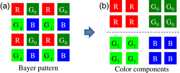
Fig. 2. Bayer pattern image and its color components.

B) Non-adaptive RCT (existing method I)

Figure 3 illustrates the RCT with fixed coefficients (existing method I) [9]. It converts four color components by

(1)$$\left[\matrix{ Y_0\cr Y_1\cr Y_2\cr Y_3 }\right]= \left[\matrix{ G_1 -G_0\cr F\lsqb \lpar R+B+F\lsqb W\rsqb \cdot 2\rpar /4\rsqb \cr R-F\lsqb W\rsqb \cr B-F\lsqb W\rsqb }\right]\comma \;$$

where

$$\left\{\matrix{ W = F\lsqb \lpar G_1 +G_0\rpar /2\rsqb \comma \; \cr F\lsqb x\rsqb = x-\lpar x \hbox{mod} \ 1\rpar }\right.$$

and F[x] denotes a floor function that converts x into integer. When the errors generated by this function is negligible, the RCT is expressed as

(2)$${\bf Y} = {\bf K}_4^T \cdot {\bf X}\comma \;$$

where

(3)$${\bf K}_4^T = \left[\matrix{ {-1} & 1 & 0 & 0\cr {1/4} & {1/4} & {1/4} & {1/4}\cr {-1/2} & {-1/2} & 1 & 0\cr {-1/2} & {-1/2} & 0 & 1 }\right]$$

and

(4)$$\eqalign{{\bf Y}& = \lsqb Y_0 \quad Y_1 \quad Y_2 \quad Y_3\rsqb ^{T}\comma \; \cr {\bf X}& = \lsqb G_0 \quad G_1 \quad R \quad B\rsqb ^{T}.}$$

Fig. 3. Non-adaptive RCT (existing method I).

Since the multiplier coefficients are fixed as expressed in (3), this RCT cannot be adaptive to each of input images.

C) Adaptive RCT (existing method II)

Figure 4 illustrates the RCT based on KLT (existing method II) [16]. The matrix K₄ in (2) is determined as eigenvectors of the covariance matrix R_X defined as

(5)$${\bf R}_{{\bf X}} = E\lsqb {\bf X}\cdot {\bf X}^T\rsqb \comma \;$$

where E[ ] denotes the ensemble average of each row and column. The KLT converts R_X to

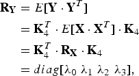(6)$$\eqalign{{\bf R}_{{\bf Y}} &= E\lsqb {\bf Y}\cdot {\bf Y}^T\rsqb \cr &= {\bf K}_4^T \cdot E\lsqb {\bf X}\cdot {\bf X}^T\rsqb \cdot {\bf K}_4\cr &= {\bf K}_4^T \cdot {\bf R}_{{\bf X}} \cdot {\bf K}_4 \cr &= diag \lsqb \lambda_{0} \, \, \lambda_{1} \, \, \lambda_{2} \, \, \lambda_{3}\rsqb \comma \; }$$

where λ_i, i ∈ {0, 1, 2, 3} denote eigenvalues. As a result, Y is decorrelated adaptively to each of input color images.

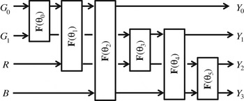
Fig. 4. Adaptive RCT (existing method II).

The 4 × 4 matrix K₄ is factorized into a product of 2 × 2 matrices

(7)$${\bf F}\lpar \theta_i\rpar = {\bf P}_t \cdot {\bf G}\lpar \varphi_{i\comma t}\rpar$$

for i ∈ {0, 1, 2, 3, 4, 5} as illustrated in Fig. 4. Each of the matrices is composed of Givens rotation

(8)$${\bf G}\lpar \varphi_{i\comma t}\rpar = \left[\matrix{ {\cos \varphi_{i\comma t}} & {-\sin \varphi_{i\comma t}}\cr {\sin \varphi_{i\comma t}} & {\cos \varphi_{i\comma t}} }\right]$$

and one of the permutations

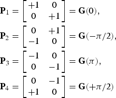(9)$$\eqalign{{\bf P}_1 & = \left[\matrix{ {+1} & 0\cr 0 & {+1} }\right]= {\bf G}\lpar 0\rpar \comma \; \cr {\bf P}_2 & = \left[\matrix{ 0 & {+1}\cr {-1} & 0 }\right]= {\bf G}\lpar -\pi/2\rpar \comma \; \cr {\bf P}_3 & = \left[\matrix{ {-1} & 0\cr 0 & {-1} }\right]= {\bf G}\lpar \pi\rpar \comma \; \cr {\bf P}_4 &= \left[\matrix{ 0 & {-1}\cr {+1} & 0 }\right]= {\bf G}\lpar +\pi /2\rpar }$$

to avoid the singular point problem [16]. Since all the rotation angles θ_i in (7) are determined according to each of input images, this RCT is adaptive.

III. PROPOSED METHOD

A) Semi-adaptive RCT and its advantages

In this paper, we propose an RCT illustrated in Fig. 5. A redundant part of the existing method II in Fig. 4 is eliminated. The rotation angle θ₀ is fixed, and the total number of rotations F is reduced from six to four. In this sense, computational load is reduced. Advantages of the proposed method are summarized as below.

Fig. 5. Semi-adaptive RCT (proposed method).

(i) The optimum angles to be included into the bit-stream are reduced from six to three (50.0%). (ii) Size of the eigenvalue problem to be solved is reduced from 4 × 4 for the six angles to 3 × 3 for the three angles (56.3%). (iii) The total number of lifting steps, which means each equation in (10), is reduced from 18 to 12 (66.7%), since one rotation contains three lifting steps. (iv) Total delay due to the lifting steps is reduced, since a lifting step waits for a calculation result of the previous lifting step. In RCT, it accumulates and causes delay from input to output. (v) Total amount of rounding error in Y _i, i ∈ {0, 1, 2, 3} is expected to be reduced, since the rounding functions which generate the error in a lifting step are reduced. We confirm it in Section IV-A. Rational of our simplification for reduction of computational load is described in Section III-C.

B) Implementation issue

To make the transform reversible in Figs 4 and 5, the rotation G(φ_i,t) in (7) is implemented in the lifting structure. In case of t = 1, output signals are calculated as

(10)$$\left\{\matrix{ x'_1 =x_1 + O\lsqb f_0 \cdot x_0 \rsqb \comma \; \cr y_0 = x_0 +O\lsqb f_1 \cdot x'_1 \rsqb \comma \; \cr y_1 =x'_1 +O\lsqb f_2 \cdot y_0 \rsqb \comma \; }\right.$$

with multiplier coefficients f ₀, f ₁, and f ₂ as illustrated in “type 1” in Fig. 6. Neglecting rounding errors generated by the rounding function O[ ], Right-hand side of (7) in the lifting structure is described as

(11)$$\lsqb y_0 \quad y_1\rsqb ^{T} = {\bf P}_t \cdot {\bf G}\lpar \phi_{i\comma t}\rpar \cdot \lsqb x_0 \quad x_1\rsqb ^{T}\comma \;$$

where

(12)$${\bf G}\lpar \varphi_{i\comma t}\rpar = \left[\matrix{ 1 & 0\cr {f_2 } & 1 }\right]\left[\matrix{ 1 & {f_1}\cr 0 & 1 } \right]\left[\matrix{ 1 & 0\cr f_0 & 1 }\right]$$

and

(13)$$\lsqb f_0 \, \, f_1 \, \, f_2\rsqb = \left[\tan {\phi_{i\comma t} \over 2}\comma \; \, \, {-\sin \phi_{i\comma t}}\comma \; \, \, \tan {\phi_{i\comma t}\over 2}\right].$$

Fig. 6. Implementation of the rotation F.

It indicates that the absolute value of f ₀ and f ₂ becomes extremely huge when the rotation angle φ_{i, t} is close to π [rad]. It magnifies rounding error, and therefore it degrades coding efficiency. This singular point problem is avoided by selecting a proper t ∈ {1, 2, 3, 4}. From (7) and (9),

(14)$$\varphi_{i\comma t} =\theta_i -\Theta_t$$

for

(15)$$\lsqb \Theta_1\ \Theta_2\ \Theta_3\ \Theta_4\rsqb = \lsqb 0 \, \, -\pi /2 \, \, \pi \, \, \pi/2\rsqb$$

is derived. Therefore, a proper t is the one which maximizes the distance between the singular point φ_i,t=π rad and the compensated angle θ_i–Θ_t. In this paper, we follow this procedure reported in [16].

C) Rational of the simplification

Firstly, the angle θ₀ in the existing method II is fixed to π/4 rad in our approach. This is because variance of G ₀ and that of G ₁ are almost the same. For example, the optimum angle θ_opt of a rotation F(θ) is given as

(16)$$\theta_{opt} = {{1} \over {2}}\left({{\pi} \over {2} }+ \arctan{ {r-1} \over {2\rho}}\right)\comma \;$$

where

(17)$$\left\{\matrix{ r = {{\sigma_{x_1}^2} \over {\sigma_{x_0}^2}}\comma \; \hfill & \rho = {{E\lsqb \lpar x_0 -\bar{x}_0\rpar \lpar x_1 -\bar{x}_1\rpar \rsqb } \over {\sigma_{x_0}^2}}\comma \; \hfill \cr \bar{x}_i =E\lsqb x_i \rsqb \comma \; \hfill & \sigma_{x_i}^2 =E\lsqb \lpar x_i -\bar{x}_i\rpar ^2\rsqb \comma \; \quad i\in \lcub 0\comma \; 1\rcub }\right.$$

for input signals x = [x ₀x ₁].

Equation (16) is derived as follows. Covariance matrix R_X of X = [x ₀x ₁] is converted to R_Y by the rotation F(θ) as

(18)$${\bf R}_{{\bf Y}} = {\bf F}^{\comma T}\lpar \theta\rpar \cdot {\bf R}_{{\bf X}} \cdot {\bf F}\lpar \theta\rpar.$$

Substituting

(19)$${\bf F}\lpar \theta\rpar = \left[\matrix{ {\cos \theta} & {-\sin \theta}\cr {\sin \theta} & {\cos \theta} }\right]\comma \; \quad {\bf R}_{{\bf X}} = \left[\matrix{ 1 & \rho\cr \rho & r }\right]\sigma_{x_0}^2\comma \;$$

we have

(20)$${{\bf R}_{{\bf Y}} \over {\sigma_{x_0}^2}} = {\bf I}_2 + \left[\matrix{ {1-c} & s\cr s & {1+c} }\right]\cdot {{r-1} \over {2}} + \left[\matrix{ s & c\cr c & {-s} }\right]\cdot \rho$$

for [c s] = [cos 2θ sin 2θ] and I₂ = [1 1]. Therefore, when it becomes uncorrelated,

(21)$$s\cdot {{r-1} \over {2}}+c\cdot \rho =0$$

holds. Since it is equivalent to

(22)$$\sqrt{\left({{r-1} \over {2}}\right)^2+\rho ^2} \cdot \cos \left(2\theta -\hbox{atctan} {{r-1} \over {2\rho}}\right)= 0\comma \;$$

we have the equation equivalent to (16) as

(23)$$2\theta_{opt} - \hbox{atctan} {{r-1} \over {2\rho}} = {{\pi}\over {2}}.$$

According to (16) and (17), θ_opt=π/4 [rad] for r = 1 in which variance of x ₀ and that of x ₁ is the same. This is experimentally endorsed for several images as summarized in Fig. 7. Note that the tested images are subsampled to generate Bayer-type four color components and used for evaluation. The angle varies depending on input images. Standard deviation was observed to be 6.58° for [x ₀x ₁] = [R B] at maximum. It is 0.20° for [x ₀x ₁] = [G ₀G ₁], namely the angle can be fixed.

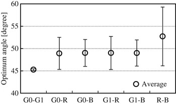
Fig. 7. Optimum angle of the rotation F(θ) for images.

Secondly, both of the angles θ₁ and θ₂ in the existing method II are set to zero. This is because variance of Y ₀ in Fig. 5 is close to zero. It comes from a fact that correlation between G ₀ and G ₁ is close to one. For example, variance of Y ₀ is given as

(24)$$\sigma_{Y_0}^2 = {{\sigma_{x_0}^2} \over {2}} \lpar 1+r-2\rho\rpar$$

for x = [x ₀x ₁]. This equation is derived as follows. Since Y ₀ is the first row of the matrix

(25)$${\bf Y} = {\bf F}^{T}\lpar \pi /4\rpar \cdot {\bf X}\comma \;$$

its variance is given as

(26)$$\sigma_{Y_0}^2 = E\left[\left({{x_0 -x_1} \over {\sqrt{2}}}\right)^2\right]= {{E\lsqb x_0^2\rsqb +E\lsqb x_1^2\rsqb -2E\lsqb x_0 x_1 \rsqb } \over {2}}\comma \;$$

which is equivalent to (24).

As described above, it becomes almost zero for r = 1 and ρ = 1. It is no use to rotate this component with other component. Therefore, rotations F(θ₁) and F(θ₂) can be eliminated. Namely, we simplified the existing method II utilizing a fact that statistical relation between the two green components G ₀ and G ₁ is fixed for various input images. The procedure itself is very simple. In the next section, we experimentally investigate its coding performance based on (1) rounding error, (2) adaptability, and (3) compaction rate.

IV. EXPERIMENTAL RESULTS

A) Rounding error

Figure 8 illustrates evaluation results of rounding errors included in Y ₀, Y ₁, Y ₂, and Y ₃. The error is defined as difference between output of an RCT with rounding function and that of the same RCT without rounding. Total amount of variance of the error is measured in peak signal to noise ratio (PSNR) defined as

(27)$${PSNR} = 10 \hbox{log}_{10} 255^2-10 \hbox{log}_{10} \sum_{i=0}^3 {\sigma_i^2}\quad \lsqb \hbox{dB}\rsqb \comma \;$$

where σ_i denotes the standard deviation of the error in Y _i. PSNR of the proposed method was observed to be 54.1 dB in average for images. It is greater than the existing method II by 2.2 dB. Reduction of the rounding functions is considered to contribute to this improvement.

Fig. 8. Evaluation of rounding error.

B) Adaptability and compaction rate

Table 1 summarizes evaluation results of data compaction rate for KODAK test images. Since this data set was reported to have considerably high correlations [19], we also used SIDBA data set and RAW images taken with Nikon D80 camera. For these images, results are summarized in Tables 2 and 3, respectively.

Table 1. The average code length of images in [bpp] for KODAK image set.

Table 2. The average code length of images in [bpp] for SIDBA image set.

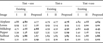
Table 3. The average code length of images in [bpp] for RAW images taken with Nikon D80 camera.

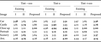
The compaction rate was measured with the average code length defined as the ratio of total amount of compressed binary data and the total number of pixels in the image. Note that it indicates 8 bit per pixel per component [bpp], when the data volume is not compressed at all. “Tint” indicates parameter of color balancing in Paint Shop Pro X3. Figures 9–11 illustrate examples of sample images at different value of “Tint”.

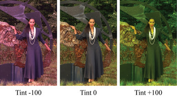
Fig. 9. Sample image “Kod05” at different value of “Tint”.

Fig. 10. Sample image “Airplane” at different “Tint”.

Fig. 11. Sample image “Scenery” at different “Tint”.

Table 4 indicates the average code length for all the images in Tables 1–3. In case of “Tint 0”, the existing method II and the proposed method are the same. Those are superior to the existing method I by 0.05 bpp. However, there is no significant difference. On the contrary, in case of “Tint +100”, the proposed method is the best, and the existing method I is the worst. The difference was observed to be 0.20 bpp in average.

Table 4. The average code length of all the images in [bpp].

Figures 12–14 illustrate the average code length of the existing method I and the proposed method for a sample image in Figs 9–11, respectively. These are subtracted by that of the existing method II. There is no significant difference between the existing method II and the proposed method. It means that the proposed method keeps adaptability of the existing method II, even though signal processing is simplified. It also indicates that the existing method I is not adaptive. This is because its multiplier coefficients are fixed as indicated in (3).

Fig. 12. The average code length subtracted by the existing method II for a sample image “Kod05”.

Fig. 13. The average code length subtracted by the existing method II for a sample image “airplane”.

Fig. 14. The average code length subtracted by the existing method II for a sample image “scenery”.

C) Discussions on improvement of compaction rate

As a result of our experiments, it was observed that the proposed method attains almost the same coding performance as the existing method II, even though its computational load is reduced. Remarkably, the proposed method is slightly better than the existing method II for greenish images with “Tint +100”. In the rest of this paper, we endorse it with theoretical analysis on entropy rate and probability density function (PDF) of signals inside the RCT.

Figure 15 illustrates the first-order entropy H, which is defined as

(28)$$H={{1} \over {4}}\sum_{i=0}^3 \sum_j W_j \cdot H_{i\comma j}\comma \;$$

where

(29)$$H_{i\comma j} =-\sum_{x_{i\comma j} } P\lpar x_{i\comma j} \rpar \hbox{log}_2 P\lpar x_{i\comma j}\rpar$$

and x _{i, j} denotes the pixel value in jth frequency band of the RWT in ith component. W _j denotes the ratio of the total number of pixels in jth band to all the number of pixels in each component. The entropy H is determined by the PDF of x _{i, j}, and it estimates the average code length illustrated in Fig. 12.

Fig. 15. The first-order entropy H subtracted by that of the existing method II for “for a sample image “Kod05”.

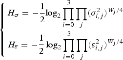
Figures 16 and 17 illustrate the sigma term H _σ and the epsilon term H_ε of the first-order entropy H, respectively. Those are defined as

(30)$$H = H_\sigma +H_\varepsilon$$

where

(31)$$\left\{\matrix{ H_\sigma =-\displaystyle{{1}\over{2}}\hbox{log}_2 \prod \limits_{i=0}^3 \prod_j \lpar \sigma_{i\comma j}^2\rpar ^{W_j /4} \cr H_\varepsilon =-\displaystyle{{1} \over {2}}\log_2 \prod \limits_{i=0}^3 \prod_j \lpar \varepsilon_{i\comma j}^2\rpar ^{W_j /4} }\right.$$

for standard deviation σ_{i, j} of x _{i, j}. A parameter ɛ_i,j is determined by shape of the PDF [20]. Figure 16 indicates that there is no difference between the existing method II and the proposed method in respect of the coding gain, which is often used for theoretical evaluation of lossless coding assuming that shape of all the PDF are the same. On the contrary, Fig. 17 indicates superiority of the proposed method to the existing method II. As a result, it was found that superiority of the proposed method comes from suitability of shape of PDF.

Fig. 16. The sigma term H _σ in the first-order entropy H. It is subtracted by that of the existing method II.

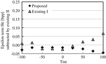
Fig. 17. The epsilon term H _ɛ in the first-order entropy H, which is subtracted by that of the existing method II. (a) Existing method II (KLD = 0.09) (b) Proposed method (KLD = 0.33).

Finally, we compare the existing method II and the proposed method in respect of shape of PDF. In Fig. 18(a), “Existing II” indicates histogram of signal values of Y ₀ in Fig. 4, and “Gaussian” indicates the Gaussian function:

(32)$$G\lpar x\rpar = {{1} \over {\sqrt{2\pi} \sigma}} \exp \left\{-\left({{\lpar x-\mu\rpar ^2} \over {2\sigma^2}}\right)\right\}$$

with zero mean μ = 0 and the same variance σ as the signal values of Y ₀. Similarly, “Proposed” in Fig. 18(b) indicates histogram of signal values of Y ₀ in Fig. 5. Comparing these figures, it is observed that “existing II” is closer to “Gaussian” than “Proposed”. This is numerically endorsed with the Kullback–Leibler divergence defined by

(33)$${KLD}\lpar P\Vert Q\rpar = \sum_k P\lpar k\rpar \log {{P\lpar k\rpar } \over {Q\lpar k\rpar }}\comma \;$$

where k denotes the pixel value. In this case, Q(k) is set to Gaussian function with the same variance as that of Y ₀. It is observed that KLD of the existing method II is 0.09, which is smaller than that of the proposed method by 0.24.

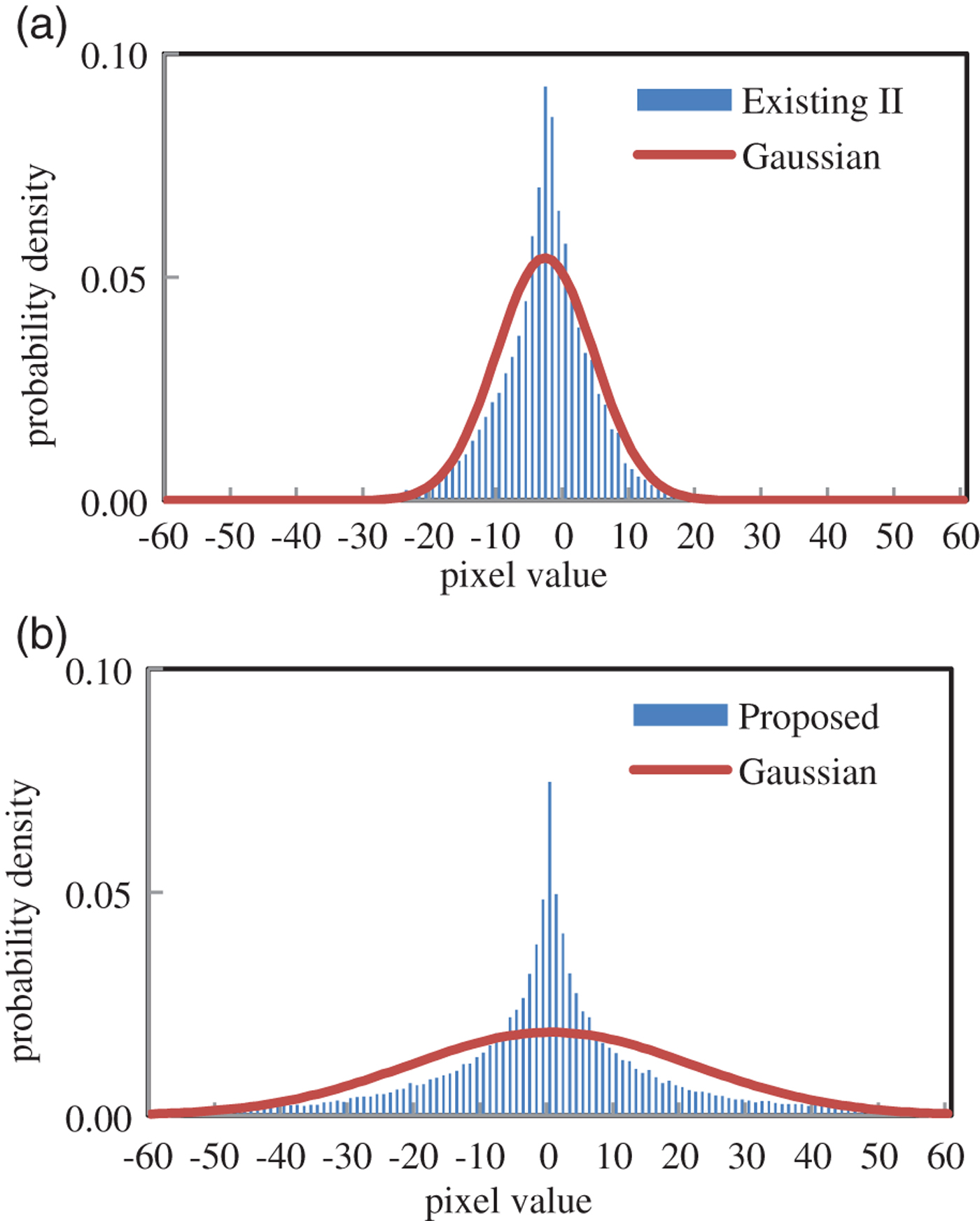
Fig. 18. PDF and KLD.

It can be considered that PDF tends to become Gaussian-like shape according to the central limit theorem in the existing method II, due to more lifting steps than the proposed method. In conclusion, it was indicated that simplification of the proposal in this paper (reduction of the number of lifting steps) keeps “good” shape of PDF, and contributes to improving coding performance. However, there is some room for further investigation.

V. CONCLUSIONS

In this paper, we simplified an existing KLT-based RCT, maintaining its adaptability to various Bayer color filter array images. We removed a redundant part of its lifting steps, utilizing a fact that G ₀ and G ₁ have almost the same variance and relatively strong correlation.

As a result, overhead to be included into the bit-stream, size of the eigenvalue problem and the total number of lifting steps are reduced to 50.0, 56.3, and 66.7%, respectively. Total amount of rounding error is confirmed to be reduced by 2.2 dB. Even though its computational load is reduced, it was observed that the proposed method attains slightly better coding performance. We endorsed it with theoretical analysis on the entropy and PDF of signals inside the RCT. However, further investigation is necessary in the future.