INTRODUCTION
As a global issue related to the global warming trend, it has been predicted that infectious diseases will increase in association with the prevalence of infectious agents such as protozoa, bacteria and viruses, as well as the spread of vector organisms, and will cause increased morbidity and mortality in many regions of the world [Reference Patz1]. The World Health Organization estimates that over the past 30 years, the warming and precipitation trends due to anthropogenic climate change have already claimed over 150 000 lives annually [Reference Campbell-Lendrum and Corvalan2]. For example, heat waves resulted in about 22 000–45 000 heat-related deaths across Europe over 2 weeks in August 2003. This is the most striking example of health risks directly resulting from short-term temperature change. Furthermore, many prevalent diseases such as cardiovascular mortality and respiratory illnesses are linked to changes in climate. Reproduction and survival rates as well as the spread of deadly vector-borne diseases are strongly affected by climatic change such as extreme weather variations occurring over weeks, months or years. Thus, elucidating the correlation between the prevalence of infectious disease incidence and climatic change occurring due to global warming is an important topical issue.
Spectral analysis is one of the powerful methods to elucidate the correlation between the prevalence of infectious disease incidence and periodicities of environmental factors. There have been a number of studies utilizing spectral analysis for time-series data of prevalence of cholera incidence as a major enteric infection in relation to sea surface temperature (SST) [Reference Pascual3–Reference Colwell7]. Those studies reported that only periodic modes of 4–5 and 3·7 years were obtained as common links between cholera incidence and El Niño [Reference Pascual3–Reference Bouma and Pascual5]. Furthermore, according to our preliminary study of cholera data, it was noted that the periodic mode of 11 years was observed as dominant modes for cholera data. As is well known, an 11-year periodic mode is clearly observed for time-series data of sunspot numbers, i.e. typical solar activity [Reference Ohtomo8–Reference Bloomfield11], and therefore the periodicity of cholera incidence is possibly related to solar activity.
In the current study, in order to investigate the comprehensive periodic structure of cholera incidence and the relationship of cholera to El Niño and solar activity as global environmental factors, we used the time-series analysis method which combined a spectral analysis based on maximum entropy method (MEM) with a nonlinear least squares method (LSM) [Reference Ohtomo8, Reference Ohtomo12–Reference Hosoda, Kasanuki and Ohtomo15].
DATA
In this study, the time-series data of cholera incidence (percent cholera cases), SST linked to El Niño-Southern Oscillation (ENSO), and Wolf's sunspot numbers were used. The cholera data were obtained from a systematic sample of the patients visiting the International Centre for Diarrhoeal Disease Research, Bangladesh (ICDDR,B) facility from January 1980 to March 1998 in Dhaka, Bangladesh [Reference Pascual3] and are summarized in Figure 1 a. The diagnosis of cholera infection has been described previously [Reference Pascual3, Reference Rodo4]. The sampling interval was 1 month and the number of data was 219.
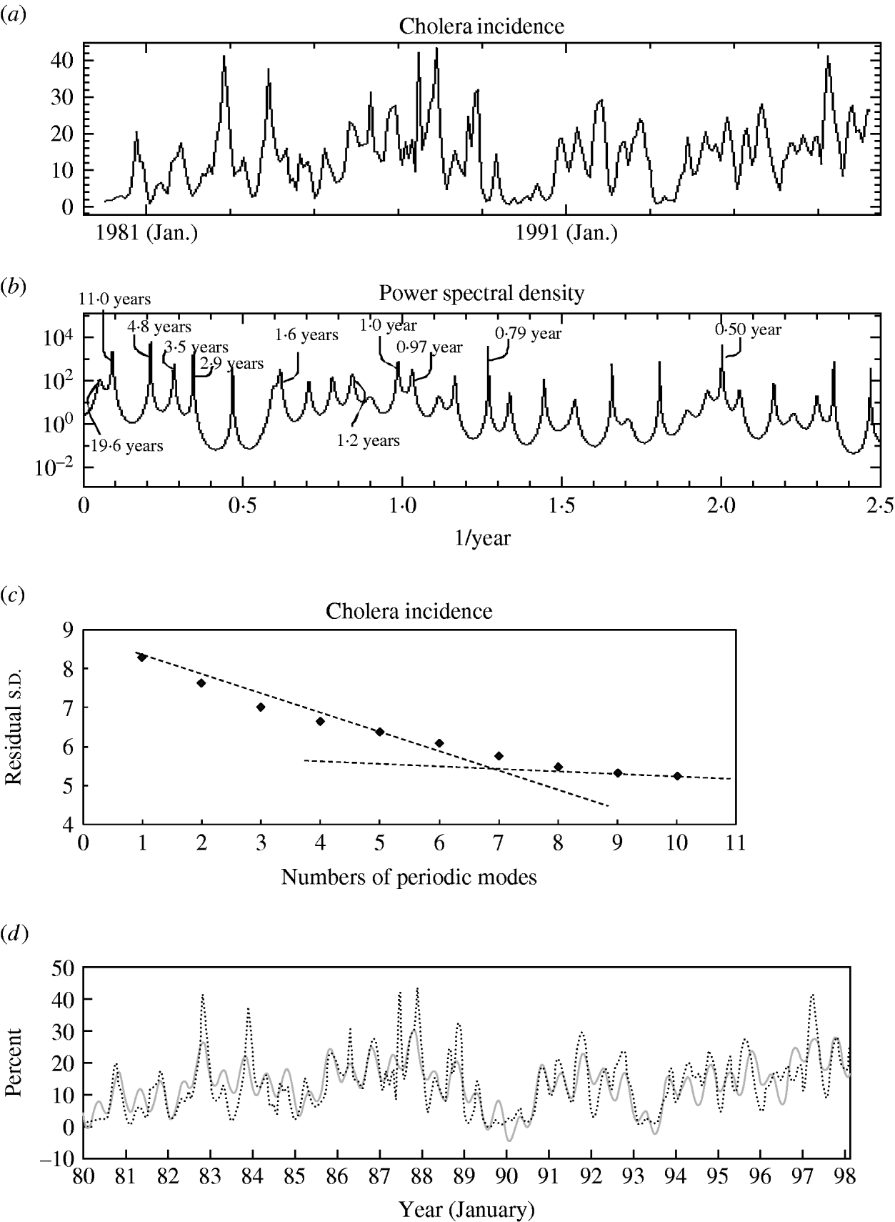
Fig. 1. Time-series data, maximum entropy method-power spectral density (MEM-PSD) and least squares fitting (LSF) for cholera incidence. (a) The original data, (b) MEM-PSD, (c) contribution of periodic modes to the LSF curve, (d) comparison of the optimum LSF curve (![]() ) with the original data (·······).
) with the original data (·······).
The SST data in the region of Niño.3 (latitude 5° N–5° S, longitude 150° W–90° W) are one of the indices for ENSO in the equatorial East Pacific (http://www.data.kishou.go.jp/climate/elNino), and are shown in Figure 2 a. The time span, the sampling interval and the number of data for SST (Niño.3) were also identical to those for cholera. Moreover, SST data in the Bay of Bengal (latitude 14° N–19° N, longitude 86° E–92° E) were also used from December 1981 to March 1998 (NASA http://poet.jpl.nasa.gov/), and the sampling interval and the number of data were 1 month and 196, respectively.
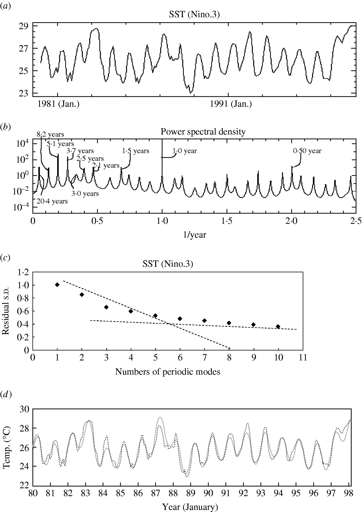
Fig. 2. Time-series data, maximum entropy method-power spectral density (MEM-PSD) and least squares fitting (LSF) for sea surface temperature (SST) (Niño.3). (a) The original data, (b) MEM-PSD, (c) contribution of periodic modes to the LSF curve, (d) comparison of the optimum LSF curve (![]() ) with the original data (·······).
) with the original data (·······).
The sunspot number data, which is one of the indices for solar activity, were obtained from the World Meteorological Organization (WMO) (http://www.wmo.int/) over the same periods as the cholera data were obtained, and confirmed by the Chronological Scientific Table [16], and are summarized in Figure 3 a. The sampling interval and the number of data were 1 month and 219, respectively, which were identical to those for cholera.
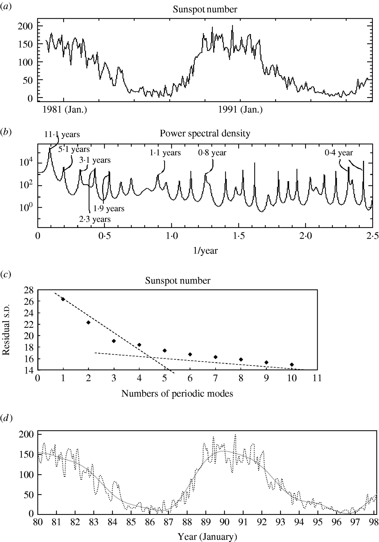
Fig. 3. Time-series data, maximum entropy method-power spectral density (MEM-PSD) and least squares fitting (LSF) for sunspot number data. (a) The original data, (b) MEM-PSD, (c) contribution of periodic modes to the LSF curve, (d) comparison of the optimum LSF curve (![]() ) with the original data (·······).
) with the original data (·······).
METHODS
A method of time-series analysis, which was used to investigate the periodic structure of cholera incidence correlated with SST and the sunspot number in this study, has been previously developed by our group [Reference Ohtomo8, Reference Ohtomo12–Reference Hosoda, Kasanuki and Ohtomo15]. This method combines MEM spectral analysis for a frequency range with the nonlinear LSM for the time range. The details have been reported previously [Reference Ohtomo8, Reference Hosoda, Kasanuki and Ohtomo15], and are briefly described as follows. This analysis was performed by the use of MemCalc (Suwa-Trast, Japan) [Reference Ohtomo8]. In addition, SPSS version 14.0J (SPSS, Japan) was used for statistical analysis.
MEM spectral analysis for frequency range
MEM power spectral density (MEM-PSD) P(f) (where f represents frequency) for the time series with equal sampling interval Δt, can be expressed by
![P\lpar \ f\ \rpar \equals {{P_{m} \rmDelta t} \over {\left\vert {1 \plus\! \sum\limits_{k \equals \minus m}^{m}\! {\gamma _{m\comma k} \exp \left[ { \minus i2\pi {\kern 1pt} f{\kern 1pt} k\rmDelta t{\kern 1pt} } \right]} } \right\vert^{\setnum{2}} }}\comma\hfill](https://static.cambridge.org/binary/version/id/urn:cambridge.org:id:binary:20160921000331225-0818:S0950268809990203:S0950268809990203_eqn1.gif?pub-status=live)
where the value of P m is the output power of a prediction-error filter of order m and γm,k the corresponding filter order. The details have been previously described [Reference Ohtomo8]. The value of the MEM-estimated period of the nth peak component T n (=1/f n; where f n is the frequency of the nth peak component) can be determined by the positions of peaks in the MEM-PSD.
LSM analysis for time range
The underlying variation of time series x UV(t) for the original time series x(t) can be expressed as a linear combination of sine and cosine functions,
where unknown parameters f n, a 0 (a constant which indicates the average value of the time series), a n and b n (n=1, 2, …, N p) (the amplitudes of the nth periodic component), and N p (the total number of components) are calculated by LSM.
The LSM using equation (2) must be nonlinear. This nonlinearity can be linearized by using the MEM-estimated periods T n and the linearization enables us to obtain unique optimum values of these parameters. Thus, the optimum values of parameters a 0, a n and b n (n=1, 2, 3, …, N p) in equation (2) are exactly determined from the optimum least squares fitting (LSF) curve calculated using equation (2) with the MEM-estimated value of T n determined in advance. x UV(t) can easily be estimated as the optimum LSF curve for the original time series. The optimum value of N p can be determined by the trend of the standard deviation (s.d.) for the residual time series x R(t), where x R(t)=x(t) – x UV(t).
RESULTS
Periodic structures
Cholera incidence data
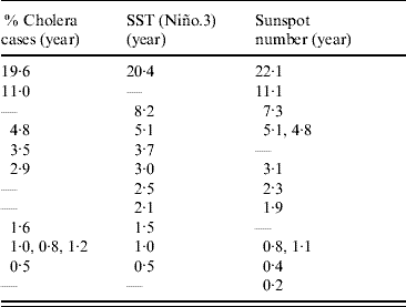
The PSD for cholera incidence data (Fig. 1 a) was calculated with the MEM spectral analysis method [equation (1)], and the result is shown in Figure 1 b. Many distinct spectral peaks are clearly observed. Ten spectral frequency modes were selected in descending order of power of spectral peak (see Table 1). Among them, the peaks at 4·8, 0·5 and 11·0 years have large spectral powers.
Table 1. Comparison of periodic modes obtained for cholera data, sea surface temperature (SST) data and sunspot number data in descending order of period
The dominant periodic modes were extracted by the following procedure. The s.d. values for x R(t) were calculated with the variation of N p and are plotted against N p in Figure 1 c. The two dotted lines are fitted to s.d. values, one of which displays a sharply decreasing trend against N p, while the other line is almost flat, resulting in random variation. An inflection point occurs at 6–7 modes. Thus, the dominant modes could be determined as seven modes: 11·0, 4·8, 3·5, 2·9, 1·6, 1·0 and 0·5 years.
The optimum LSF curve to the cholera data was calculated with these dominant modes and is illustrated as a solid grey line (Fig. 1 d). The LSF curve reproduces the underlying variation of the original time series well, although it does not fully reproduce short-term variations of the original time series.
SST (Niño.3) data
Similar to the cholera data, 10 periodic modes obtained from the PSD peaks for SST (Niño.3) data (Fig. 2 a) are also listed in Table 1, and six dominant modes were thus determined through the s.d. values with the variation of N p (Fig. 2 c) as 5·1, 3·7, 2·5, 2·1, 1·5, and 1·0 years. The peaks with high power ratio are the 1·0-, 5·1- and 3·7-year modes. The optimum LSF curve to the SST calculated with those dominant modes reproduces well the underlying variation of original time series (Fig. 2 d).
Sunspot number data
As for the case of cholera data, 10 or more periodic modes obtained from the PSD peaks for the sunspot number (Fig. 3 a) were compared with those for cholera as well as SST (Table 1). These periods for sunspot numbers were consistent with those for cholera, and five dominant modes were determined as 22·1, 11·1, 7·3, 4·8 and 3·1 years. The peak with the highest power ratio was observed at the 11-year mode (Fig. 3 b). The optimum LSF curve calculated with those dominant modes accurately reproduces the underlying variation of the original time series (Fig. 3 d).
Comparison of periodicity between cholera incidence and SST
Many dominant periods for cholera data and those for SST (Niño.3) were essentially consistent with each other (Table 1). The 4·8-year mode with the highest power of PSD peak, 0·5- and 11·0-year modes with the second highest power, and 3·5- and 2·9-year modes were observed for cholera incidence rates in the current study. The main periodic modes, 4·8 and 0·5 years for cholera, correspond to the 5·1- and 0·5-year modes for SST, respectively, and the 3·5- and 2·9-year modes for cholera correspond to the 3·7- and 3·0-year modes for SST, respectively. However, the other main periodic mode, 11 years for cholera (Fig. 1 b), was not detected in SST (Fig. 2 b).
In order to investigate a correlation between cholera and SST (Niño.3) data, the LSF curves were calculated with two shorter-term periodic modes (1·0 and 0·5 years), and the LSF curves normalized in amplitude for both data were overlapped (data not shown). The curve for cholera data expressed a bimodal seasonal cycle with a small peak in spring and a large one in autumn or early winter. On the other hand, the LSF curve for SST has a single cycle with a 1-year mode and displays the peak in spring, where the peak precedes the large peak for cholera incidence by about 7 months. The correlation coefficients of Spearman's ρ and Kendall's τb for these curves were calculated, respectively, where significant levels were P<0·05 and P<0·001. The shorter-term periodic mode did not show significant correlation (ρ=−0·101, P<0·05 and τb=−0·075, n.s.).
In order to confirm the origin of the shorter-term cycle of cholera incidence, we examined SST data at the Bay of Bengal, close to Bangladesh. The LSF curve for SST (Bengal) calculated with 1·0- and 0·5-year periodic modes ascertained the bimodal periodic structure of SST (Fig. 4 a). This result showed a positive significant correlation with the case of cholera (ρ=0·149 and τb=0·109, P<0·05).
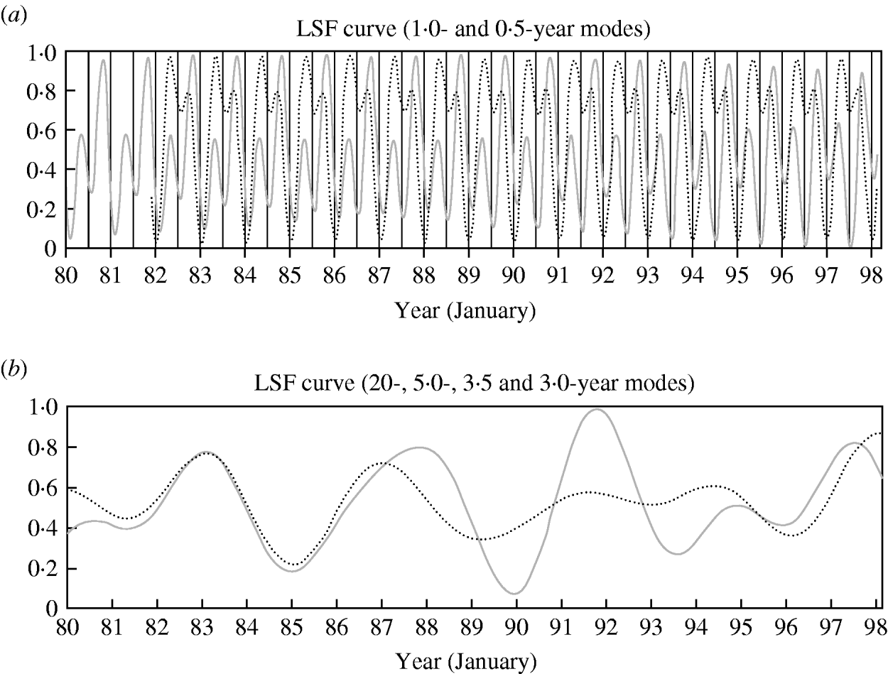
Fig. 4. Comparison of the normalized least squares fitting (LSF) curves for cholera data (![]() ) and sea surface temperature (SST) data (·······). The result was calculated for SST data in the Bay of Bengal by using the shorter-term periodic modes (1 and 0·5 years). The result was calculated for SST data in Niño.3 by using the longer-term periodic modes (20, 5, 3·5, 3·0 years).
) and sea surface temperature (SST) data (·······). The result was calculated for SST data in the Bay of Bengal by using the shorter-term periodic modes (1 and 0·5 years). The result was calculated for SST data in Niño.3 by using the longer-term periodic modes (20, 5, 3·5, 3·0 years).
The LSF curves with four longer-term periodic modes, 20·0, 5·0, 3·5 and 3·0 years, were calculated for cholera and SST (Niño.3) data; the normalized LSF curves are shown in Figure 4 b. Both curves were in-phase between cholera and SST (Niño.3) data with a positively significant correlation (P<0·001).
Comparison of periodicity between cholera incidence and sunspot numbers
Eleven-year and 4·8-year modes for sunspot number data showed the stronger power, as for cholera. In order to investigate a correlation between cholera and sunspot number data, the LSF curves with 11·0- and 4·8-year modes were calculated, and these curves normalized in amplitude were overlapped as shown in Figure 5(a, b), respectively. In both LSF curves, the oscillation is shown in opposite phases between cholera and sunspot number data with a significant correlation (P<0·001). The correlation coefficients (ρ and τb) for these curves are strongly negative (Table 2).
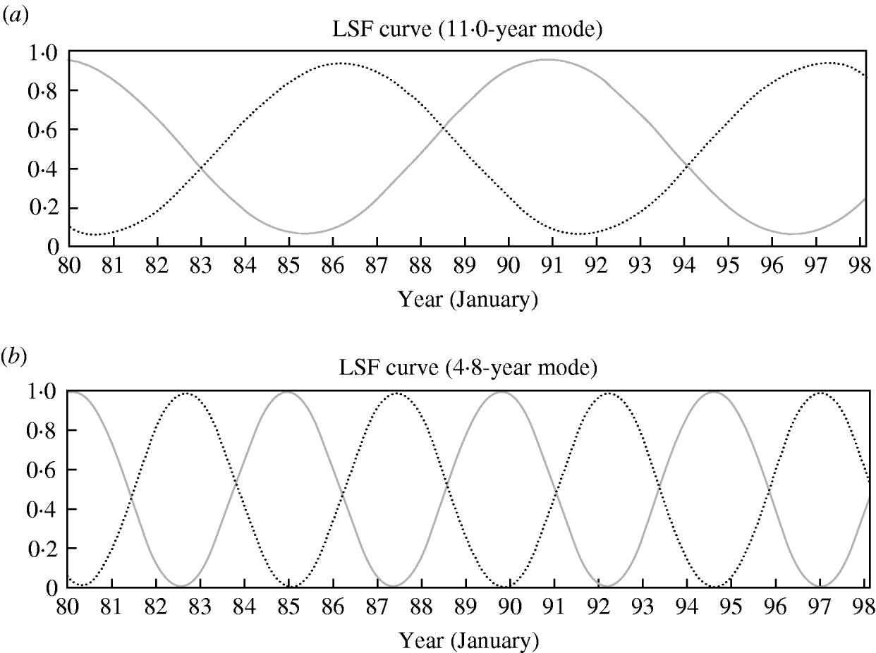
Fig. 5. Comparison of the normalized least squares fitting (LSF) curves for cholera data (![]() ) and sunspot number data (·······). (a) The result calculated by using the 11-year mode. (b) The result calculated by using the 4·8-year mode.
) and sunspot number data (·······). (a) The result calculated by using the 11-year mode. (b) The result calculated by using the 4·8-year mode.
Table 2. Correlation coefficients calculated for raw data and least squares fitting (LSF) curves with shorter-term and longer-term periodic modes
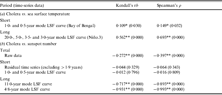
Significant levels: ** P<0·001, * P<0·05.
DISCUSSION
Time variation of cholera incidence data
The LSF curve for cholera data did not fully reproduce the fine structure of time variation of the original data, but that for SST data accurately reproduced the time variation of the original data. This difference is considered to be caused by the following reasons. The time variation of SST data is based on a physical relaxation phenomenon induced by the variation of solar light volume, which is a slow variation with the periodicity from several months to years. On the other hand, cholera incidence is a complicated biological phenomenon affected by various social factors. It is possible that Vibrio cholerae increases explosively under conditions that cause increases to optimal temperatures and the presence of rich nutrients in water. Additionally, shorter-term variations of cholera incidence fluctuate under the conditions of population density as well as the status of immunity in individuals [Reference Lipp, Huq and Colwell17]. Thus, these various factors would give unpredictable variations to cholera data as shorter-term periodic or non-periodic modes.
Longer-term periodic structure of the sunspot number and SST (Niño.3) influencing cholera
Bouma & Pascual also reported the existence of a 10-year mode from cholera mortality [Reference Bouma and Pascual5], and described how ‘this decadal inter-annual variation in the dynamics of cholera remains unexplained by current environmental hypotheses’. In our study, an 11-year mode was identified for the first time, although a 10-year mode was not observed. It is suggested that such differences may be caused by difference of original data and methodology; we used cholera incidence data and employed MemCalc software, which is a linearized version of the nonlinear LSM combined with the maximum entropy spectral analysis method. We considered that the 11-year mode for cholera incidence results may be associated with the well-known 11-year cycle observed for solar activity [Reference Ohtomo8], i.e. sunspot number.
Interestingly, the 11-year mode for cholera data was correlated in an opposite phase to that for sunspot number data: cholera incidence increases as solar activity (the sunspot number) decreases, and vice versa. The same characteristic was also observed for the 4·8-year mode. These findings suggest that the increase of solar radiation, which is associated with an increase of ultraviolet (UV) radiation, may have an elevated bactericidal effect in nature, resulting in a decrease of cholera incidence [Reference Faruque18–Reference Conroy20].
On the other hand, the longer-term periodic relationship between cholera incidence and SST (Niño.3) variation was discovered to be in phase with each other. This fact is considered to be related to an increase of marine plankton as suggested previously [Reference Bouma and Pascual5].
Shorter-term periodic structure of SST influence on cholera
Regarding the 0·5-year mode [=frequency of 2 (1/year)] observed for cholera data with a bimodal seasonal cycle, it is important to investigate whether the 0·5-year mode is a harmonic component of the 1-year mode. This 0·5-year mode is apparently a dominant peak mode because of the same spectral power level as that of the 1-year mode for cholera. Conversely to the case of cholera, the 0·5-year mode for SST in Niño.3 has a low power value (only 4% power level to 1-year mode). Thus, the 0·5-year mode for SST is considered to be a harmonic component in the case of Niño.3. This is supported by the fact that the SST waveform of Niño.3 was substantially sinusoidal and the harmonic components had minimal power.
The SST in the region of Niño.3 shows only a single peak in spring, and this SST peak precedes the large cholera peak by about half a year. This finding may be consistent with the fact that the rise of SST in the Indian Ocean occurs about 2–4 months after the peak of El Niño.
In contrast, the SST in the Bay of Bengal shows annual bimodal peaks, and these SST peaks are consistent with cholera peaks. While the SST peaks in the latter half of the year are smaller than those in the first half, peaks of cholera become larger in autumn or winter than in spring. Although the reason for this inconsistency between SST and cholera is unknown, it appears that SST may not be solely related to cholera prevalence.
One possible reason for this is that the intensity of solar radiation may have an influence on cholera prevalence [Reference Faruque18–Reference Conroy20], in addition to SST. The survival of bacteria is possibly affected by UV from solar radiation which has bimodal peaks in Dhaka and reaches a maximum level in spring, especially March–May.
The results of the current study suggest that cholera incidence in Bangladesh may have been influenced by the occurrence of El Niño and also by the periodic change of solar activity. Further time-series analyses of cholera and meteorological data in other regions of the world may elucidate the possible relatedness between the cholera epidemics and El Niño/solar activities, or other environmental factors.


