Environmental sound recognition: a survey

Abstract

Although research in audio recognition has traditionally focused on speech and music signals, the problem of environmental sound recognition (ESR) has received more attention in recent years. Research on ESR has significantly increased in the past decade. Recent work has focused on the appraisal of non-stationary aspects of environmental sounds, and several new features predicated on non-stationary characteristics have been proposed. These features strive to maximize their information content pertaining to signal's temporal and spectral characteristics. Furthermore, sequential learning methods have been used to capture the long-term variation of environmental sounds. In this survey, we will offer a qualitative and elucidatory survey on recent developments. It includes four parts: (i) basic environmental sound-processing schemes, (ii) stationary ESR techniques, (iii) non-stationary ESR techniques, and (iv) performance comparison of selected methods. Finally, concluding remarks and future research and development trends in the ESR field will be given.

I. INTRODUCTION

A considerable amount of research has been made toward modeling and recognition of environmental sounds over the past decade. By environmental sounds, we refer to various quotidian sounds, both natural and artificial (i.e. sounds one encounters in daily life other than speech and music). Environmental sound recognition (ESR) plays a pivotal part in recent efforts to perfect machine audition.

With a growing demand on example-based search such as content-based image and video search, ESR can be instrumental in efficient audio search applications [1]. ESR can be used in automatic tagging of audio files with descriptors for keyword-based audio retrieval [2]. Robot navigation can be improved by incorporating ESR in the system [3, 4]. ESR can be adopted in a home-monitoring environment, be it for assisting elderly people living alone in their own home [5, 6] or for a smart home [7]. ESR, along with image and video analysis, find applications in surveillance [8, 9]. ESR can also be tailored for recognition of animal and bird species by their distinctive sounds [10, 11].

Among various types of audio signals, speech and music are two categories that have been extensively studied. In its infancy, ESR algorithms were a mere reflection of speech and music recognition paradigms. However, on account of considerably non-stationary characteristics of environmental sounds, these algorithms proved to be ineffective for large-scale databases. For example, the speech recognition task often exploits the phonetic structure that can be viewed as a basic building block of speech. It allows us to model complicated spoken words by breaking them down into elementary phonemes that can be modeled by the hidden Markov model (HMM) [12]. In contrast, general environmental sounds, such as that of a thunder or a storm, do not have any apparent sub-structures such as phonemes. Even if we were able to identify and learn a dictionary of basic units (analogous to phonemes in speech) of these events, it would be difficult to model their variation in time with HMM as their temporal occurrences would be more random as against preordained sequence of phonemes in speech. Similarly, as compared with music signals, environmental sounds do not exhibit meaningful stationary patterns such as melody and rhythm [13]. To the best of our knowledge, there was only one survey article on the comparison of various ESR techniques done by Cowling and Sitte [14] about a decade ago.

Research on ESR has significantly increased in the past decade. Recent work has focused on the appraisal of non-stationary aspects of environmental sounds, and several new features predicated on non-stationary characteristics have been proposed. These features, in essence, strive to maximize their information content pertaining to signal's temporal and spectral characteristics as bounded by the uncertainty principle. For most real life sounds, even these features exhibit non-stationarity when observed over a long period of time. To capture these long-term variations, sequential learning methods have been applied.

It becomes evident that ESR methods not only have to model non-stationary characteristics of sounds, but also have to be scalable and robust as there are numerous categories of environmental sounds in real-life situations. Despite increased interest in the field, there is no single consolidated database for ESR, which often hinders benchmarking of these new algorithms.

In this work, we will present an updated survey on recent developments and point out the future research and development trends in the ESR field. In particular, we will elaborate on non-stationary ESR techniques. The rest of this paper is organized as follows. We will first discuss three commonly used schemes for environmental sound processing in Section II. Then, we will conduct a survey on stationary and non-stationary ESR techniques in Sections III and IV, respectively. In Section V, we will present experimental comparison of selected few methods. Finally, concluding remarks and future research trends will be given in Section VI.

II. ENVIRONMENTAL SOUND-PROCESSING SCHEMES

Before delving into the details of various ESR techniques, we will first describe three commonly used environmental sound-processing schemes in this section.

1) Framing-based processing

Audio signals to be classified are first divided into frames, often using a Hanning or a Hamming window. Features are extracted from each frame and this set of features is used as one instance of training or testing. A classification decision is made for each frame and, hence, consecutive frames may belong to different classes. A major drawback of this processing scheme is that there is no way of selecting an optimal framing-window length suited for all classes. Some sound events are short-lived (e.g. gun-shot) as compared with other longer events (e.g. thunder). If the window length is too small, then the long-term variations in the signal would not be well captured by the extracted features, and the framing method might chop events into multiple frames. On the other hand, if the window length is too large, it becomes difficult to locate segmental boundaries between consecutive events and there might be multiple sound events in a single frame. Also, one has to rely on features to extract non-stationary attributes of the signal since such a model does not allow the use of sequential learning methods.

2) Sub-framing-based processing

Each frame is further segmented into smaller sub-frames, usually with overlap, and features are extracted from each sub-frame. In order to learn a classifier, features extracted from sub-frames are either concatenated to form a large feature vector or averaged so as to represent a single frame. Another possibility is to learn a classifier for each sub-frame and make a collective decision for the frame based on class labels of all sub-frames (e.g., a majority voting rule). This model allows the use of both non-stationary features and sequential classifiers. Even with a non-sequential classifier, this processing scheme can represent each frame better as the collective distribution over all sub-frames allows one to model intra-frame characteristics with greater accuracy. This method offers more flexibility in segmenting consecutive sound events based on class labels of sub-frames.

3) Sequential processing

Audio signals are still divided into smaller units (called a segment), which is typically of 20–30 ms long with 50% overlap. The classifier makes decisions on class labels and segmentation both based on features extracted from these segments. As compared with the above two methods, this method is unique in its objective to capture the inter-segment correlation and the long-term variations of the underlying environment sound. This can be achieved using a sequential signal model such as the HMMs.

Any ESR algorithm basically follows one of the above three processing schemes with minor variations in its preprocessing and feature selection/reduction schemes. For example, a pre-emphasis filter can be used to boost the high-frequency content or an A-weight filter can be used for equalized loudness. For feature selection/reduction, there is an arsenal of tools to choose from [15–17]. We will not pay attention to these minor differences in later sections.

III. STATIONARY ESR TECHNIQUES

Features developed for speech/music-based applications have been traditionally used in stationary ESR techniques. These features are often based on psychoacoustic properties of sounds such as loudness, pitch, timbre, etc. A detailed description of features used in audio processing was given in [18], where a novel taxonomy based on the properties of audio features was provided (see Fig. 1).

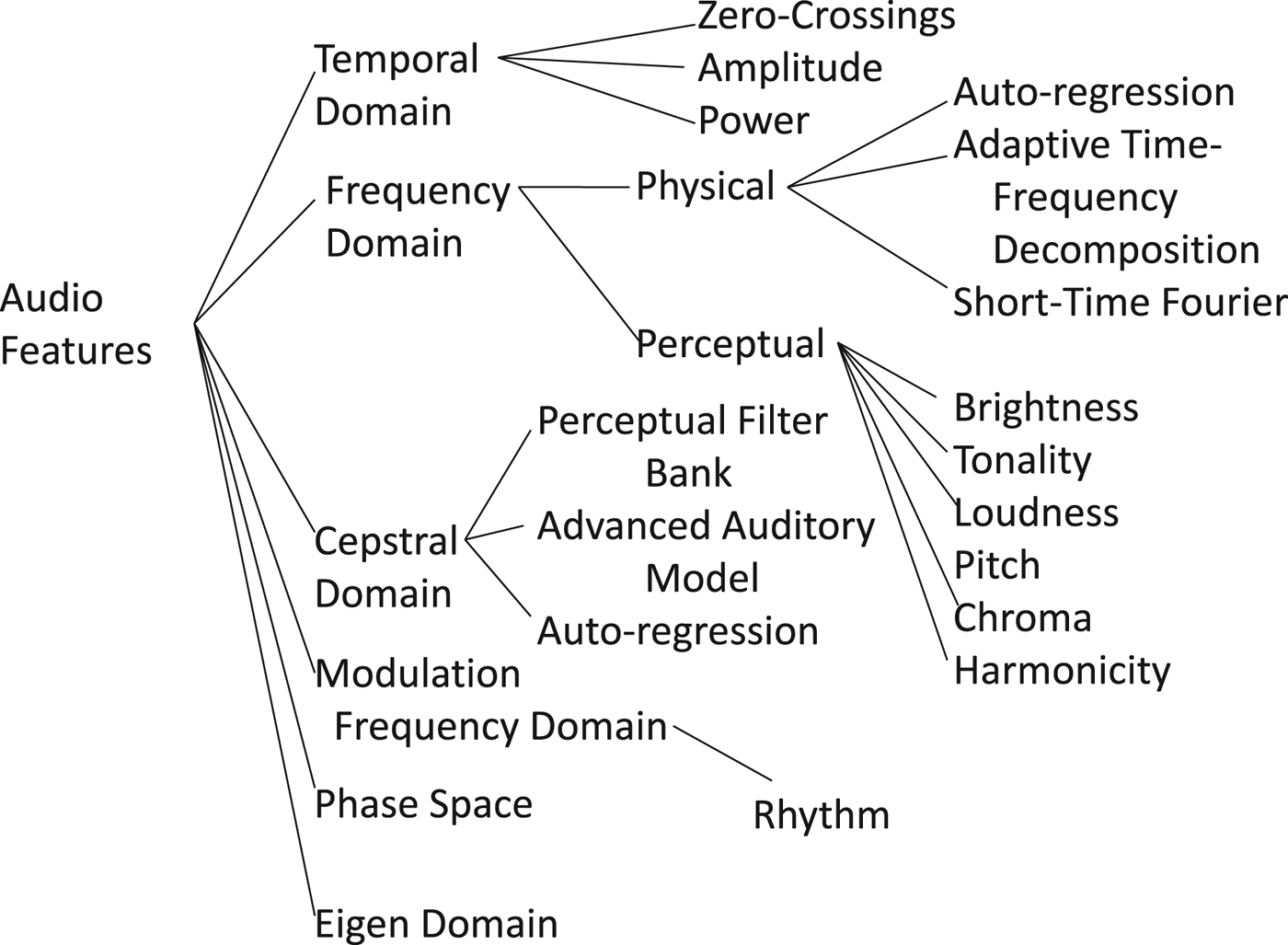
Fig. 1. Taxonomy for audio features as proposed in [18].

Features such as zero-crossing rate (ZCR), short-time energy (STE), sub-band energy ratio, spectral flux, etc. are easy to compute and used frequently along with other refined set of features. These features provide rough measures about temporal and spectral properties of an audio signal. For more details on basic features, we refer to [18–21].

Cepstral features are widely used features. They include: Mel-Frequency Cepstral Coefficients (MFCC) and their first and second derivatives (ΔMFCC and ΔΔMFCC), Homomorphic Cepstral Coefficients (HCC), Bark- Frequency Cepstral Coefficients (BFCC), etc. MFCC were developed to resemble the human auditory system and have been successfully used in speech and music applications. As mentioned before, due to lack of a standard ESR database, MFCC are often used by researchers for benchmarking their work. A common practice is to concatenate MFCC features with newly developed features to enhance the performance of a system.

MPEG-7 based features are also popular for speech and music applications. They demand low computational complexity and encompass psychoacoustic (or perceptual-based) audio properties. Wang et al. [22] proposed to use low-level audio descriptors such as Audio Spectrum Centroid and Audio Spectrum Flatness with a hybrid classifier constituted of support vector machine (SVM) and K-nearest neighbors (KNN). They converted the classifier outputs from SVM and KNN into probabilistic scores and fused them to improve classification accuracy. Muhammad et al. [23] combined several low-level MPEG-7 descriptors and MFCC and used Fisher's discriminant ratio (F-ratio) to discard irrelevant features. Although MPEG-7 features perform better than MFCC, MFCC, and MPEG-7 descriptors are shown to be complementary to each other and, when used together, the classification accuracy can be improved.

Autoregression based features, in particular, Linear Prediction Coefficients (LPC), have been prevalent in speech processing applications. Linear Prediction Cepstrum Coefficients (LPCC), which are an alternate representation of LPC, are also commonly used. However, LPC and LPCC embody the source-filter model for speech and, hence, they are not useful for ESR. Tsau et al. [24] proposed the use of the Code Excited Linear Prediction (CELP) based features along with the LPC, pitch and pitch gain features. Since CELP uses a fixed codebook for excitation of a source-filter model, it is more robust than LPC. Tsau et al. [24] reported improved performance over MFCC. CELP and MFCC together further increase the classification accuracy, specially noticeable for classes such as rain, stream, and thunder which are difficult to recognize.

ESR algorithms relying on the sub-framing processing scheme usually learn signal-models in each sub-frame and, thus, do not utilize the temporal structure. One variation to exploit the temporal structure is when a signal-model is learned based on features from all ordered sub-frames such as HMM. Another example was recently proposed by Karbasi et al. [25], which attempted to capture the temporal variation among sub-frames in a new set of features called “Spectral Dynamic Features (SDF)” as detailed below.

Let x _sb (i) denote the ith sub-frame, with i ∈ [1, N]. From each sub-frame x _sb (i), MFCC and other features are extracted in a vector y _i with dimension L × 1. Let Y = [y ₁,…,y _N ] be a matrix with columns y _i of feature vectors for N sub-frames. For each row of Y, the N-point FFT is applied followed by the logarithmic filter bank, and then followed by the N-point DCT to yield the final set of features. This method essentially extracts cepstral features (MFCC-like features) considering each row of Y as a time series. For example, if 13 MFCC coefficients are extracted from each sub-frame, then we end up with 13 time series, one for each dimension. The cepstral features are evaluated for each of these time series by capturing the dynamic variation of sub-frame features over the entire frame. The superior performance of SDF against several conventional features such as ZCR, LPC, MFCC under three classifiers (i.e., KNN, GMM, and SVM) was demonstrated. It was shown in [25] that the combined features of MFCC and ΔMFCC give the performance bound of static features, which is not improved by adding more conventional features. A system with a feature vector consisting of ZCR, Band-Energy, LPC, LPCC, MFCC, and ΔMFCC, performs poorly as compared to that with only MFCC and ΔMFCC under the SVM or GMM classifiers. In contrast, the dynamic feature set, SDF, achieves an improvement of 10–15% over the static bound.

Filter-banks are often used to extract features local to smaller bands, encapsulating spectral properties effectively. On the other hand, the auto-correlation function (ACF) represents the time-evolution and has an intimate relationship with the power spectral density (PSD) of the underlying signal. Valero and Alias [26] proposed a new set of features called the Narrow-Band Auto Correlation Function features (NB-ACF). The extraction of NB-ACF features can be explained using Fig. 2. First, a signal is passed through a filter bank with N = 48 bands whose center frequencies being tuned to the Mel-scale. Then, the sample ACF of the filtered signal in the ith band is calculated, which is denoted by Φi(τ). One can calculate four NB-ACF features based on each ACF as follows.

1. (i) Φ _i (0): Energy at lag τ = 0. It is a measure of the perceived sound pressure at the ith band.

2. (ii) τ _{i 1} : Delay of the first positive peak which represents the dominant frequency in the ith band.

3. (iii) Φ _{i 1} (τ _{i 1} ): Normalized ACF of the first positive peak. It is related to the periodicity of the signal and, hence, gives a sense of pitch of the filtered signal at the ith band.

4. (iv) τ _{i e} : Effective duration of the envelope of normalized ACF. It is defined as the time taken by normalized ACF to decay 10 dB from its maximum value, and it is a measure of reverberation of the filtered signal at the ith band.

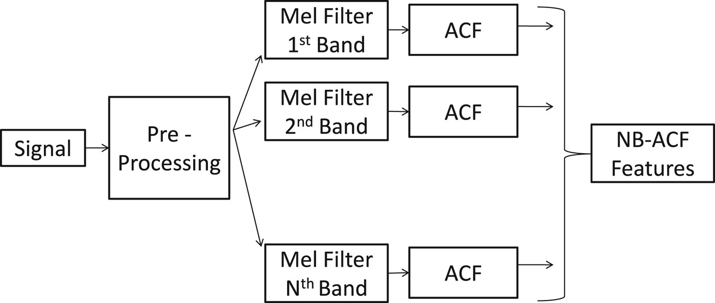
Fig. 2. Illustration of the NB-ACF feature extraction process.

As a rule of thumb, the sample ACF is meaningful up to lag τ _opt if and only if the signal length is at least four times the lag length. This demands a sub-frame length to be much larger than that used in sub-framing processing. It is recommended in [26] that a be sub-frame of size 500 ms with an overlap of 400 ms in a frame of 4 s. Finally, KNN and SVM classifiers are used for decision making in each sub-frame. The performance of NB-ACF features was compared with MFCC and discrete wavelet transform (DWT) coefficients with a data-set consisting of 15 environmental scenes. Dynamically changing scenes, such as office, library, and classroom, pronouncedly benefited from the new NB-ACF features. It is well known that ACF is instrumental in the design of linear predictors for time-series because they capture the temporal similarity/dissimilarity well. As a result, the NB-ACF features offer better performance for wide-sense-stationary (WSS) signals than most static features discussed in this section.

IV. NON-STATIONARY ESR TECHNIQUES

Any signal can be analyzed in both time and frequency domain. Both these signal representations provide different perspectives of a signal from a physical standpoint. Time information gives exact measurable representation of signal, be it vibrations as in case of audio, or light and color intensities in case of images, and so on. On the other hand, Frequency-domain methods such as Fourier transform gives an idea of average power over various constituent frequencies of the signal, thereby describing the nature of the physical phenomenon constituting the signal. However, the analysis tools when restricted to only one domain, take measurements with the assumption that the progenitorial phenomena responsible for signal production do not vary with time. Thus, features extracted using these tools work well when this assumption of “stationarity” is satisfied. However, as discussed before, real-life audio signals often violate this assumption. Such signals are assumed to have time varying characteristics, and thus such signals can be described as “non-stationary”. A class of tools, known as time–frequency analysis methods, are employed when dealing with such signals. In the following sections, we will discuss features derived from such time–frequency analysis tools.

A) Wavelet-based methods

For decades, wavelet transforms have been used to represent non-stationary signals since they offer representation in both time and frequency space. As compared to Fourier transform, which uses analytic waves to decompose a signal, wavelet transforms use “wavelets” which are nothing but “short waves” with finite energy [27]. Time-varying frequency analysis of a signal is made possible by the finite-energy property of these wavelets. An analytic function, Ψ(t) must satisfy following conditions:

• • A wavelet must have finite energy

  (1) $$\vint_{-\infty}^{+\infty}{\vert \Psi\lpar t\rpar \vert^2 dt} \lt \infty\comma \;$$

• • The admissibility condition [28] must be met by the Fourier transform of the wavelet, Ψ(ω)

  (2) $$\vint_{0}^{\infty}{\vert{\bf \Psi}\lpar \omega\rpar \vert^2 \over \omega} df \lt \infty.$$

Such an analytic function is admissible as a “mother wavelet” and can be used to generate daughter wavelets by scaling and shifting, thereby enabling more accurate localization of signal in time–frequency space. Together these functions can be used to decompose a given signal to give time-varying frequency profile.

The performance of commonly employed features for audio recognition, including Mel-Frequency Cepstral Coefficients (MFCC), Homomorphic Cepstral Coefficients (HCC), time–frequency features derived using short-term Fourier transform (STFT), DWT, and continuous wavelet transform (CWT) was compared by Cowling and Sitte in [14], where the learning vector quantization (LVQ), Artificial Neural Networks, dynamic time warping (DTW), and Gaussian Mixture Models (GMM) were used as classifiers. The experiments were conducted on three types of data – speech, music and environmental sounds. For the environmental sound, the data set consisted of eight classes, and the framing-based processing scheme was adopted. It was reported that the best performance for ESR was achieved with CWT features with the DTW classifier, which was comparable to that of MFCC features with the DTW classifier. It is surprising that CWT, which is a time–frequency representation, and MFCC gave very similar results, whereas DWT and STFT did not give good performance. It was noted in [14] that the dataset was too small to make any meaningful comparison between MFCC and CWT. Given other factors being equal, MFCC features can be more favored than CWT features because of their lower computational complexity. DTW was clearly the best classifier in the test, yet the claim should be further verified by a larger environmental sound database.

Han and Hwang [29] used the discrete chirplet transform (DChT) and the discrete curvelet transform (DCuT) along with several other common features such as MFCC, ZCR, etc. When compared, all features gave similar performance, yet significant improvement was observed when they were used together.

Valero and Alias [30] adapted the Gammatone mother function to meet wavelet admissibility conditions, used the squared sum of Gammatone representations of signal as features, called the Gammatone wavelet features, and adopted the SVM classifier. A comparable performance was observed between Gammatone wavelet features and DWT. When both features were used together, classification accuracy was improved even in noisy conditions. Gammatone features perform well in classes such as footsteps and gunshots due to their capability in characterizing transient sounds.

Umapathy et al. [31] proposed a new set of features based on the binary wavelet packet tree (WPT) decomposition. More recently, Su et al. [32] used a similar approach to recognize sound events in an environmental scene consisting of many sound events. This ESR algorithm was conducted with the framing-based processing scheme. The signal in the ith frame, x _i , is first transformed to a binary WPT representation denoted by Ω _{j, k} , where j is the depth of the tree and k is the node index at level j. Each subspace Ω _{j, k} is spanned by a set of basis vectors $\lcub {\bf{w}}_{j\comma k\comma l} \rcub_{l=0}^{2^{u}-1}$ , where 2 ^u is the length of x _i . Then, we have

(3) $$x_i =\sum_{j\comma k\comma l}\lsqb \alpha_{j\comma k\comma l}\rsqb _i \, {\bf{w}}_{j\comma k\comma l}\comma \;$$

where α _j,k,l is the projection coefficient at node (j, k). Once all training samples are decomposed to a binary WPT, the local discriminant bases (LDB) algorithm is used to identify the most discriminant nodes of the WPT. The LDB algorithm can be simply described below. For each pair of classes in the dataset, one can determine a set of Q discriminatory nodes based on a dissimilarity measure. Two dissimilarity measures were proposed in [32]:

1. (i) The difference of normalized energy

   $$D_{1}=E_{1}^{\lpar j\comma k\rpar }-E_{2}^{\lpar j\comma k\rpar }$$
   of the two sound classes at the same node (j, k);

2. (ii) The ratio of the variances of projection coefficients of the two sound classes at node (j, k),

   $$D_{2}={\rm var}\lsqb {\bf{v}}_1^{\lpar j\comma k\rpar }\rsqb /{\rm var}\lsqb {\bf{v}}_2^{\lpar j\comma k\rpar }\rsqb \comma \;$$
   where v _i ^(j,k) is the vector of variance of locally grouped coefficients at node (j, k).

Strictly speaking, none of these two dissimilarity measures are distance metrics. The selected Q nodes should be consistent. It was recommended to conduct multiple trials with randomly selected training samples from two classes, and consistent nodes should be selected from these random trials. The above process should be repeated among all possible class pairs. Finally, we select H nodes that occur most frequently among the Q nodes for each pair, and use coefficients and/or dissimilarity measure quantities at these H nodes as features.

The LDA-based classifier was used in [31] whereas the KNN and HMM were used in [32]. It was observed in [31] that WPT–LDB and MFCC features gave similar performance, yet much better performance was achieved when the two were combined together. It was reported in [32] that MFCC performed better than WPT–LDB, and a significant improvement could be obtained by combining the two features. Note that the classification performance in [32] was given for environmental scenes rather than individual events.

Despite being time–frequency features, the performance of wavelet features is not better than that of MFCC features but at a comparable level. When being combined with MFCC, the performance does improve yet the required complexity overhead to extract wavelet features might not always justify the gain in classification accuracy except for the Gammatone features. The Gammatone features are proved to be complementary to MFCC owing to their strong capability in representing impulsive signal classes such as footsteps and gun-shots.

B) Sparse-representation-based methods

Chu et al. [33] proposed to use the matching pursuit (MP)-based features for ESR. The basis MP (BMP) is a greedy algorithm used to obtain a sparse representation of signals based on atoms in an overcomplete dictionary. Given signal x and an overcomplete dictionary D=[d ₁, d ₂, …], BMP obtains the sparse representation of x on D as follows.

1. (i) Initialize the residue at the 0th iteration as R ⁰ x = x.

2. (ii) For t = 1 to T

   1. (a) Select the atom with the largest inner product with the residue via

      $$d_t = \max_{i}\langle R^{t-1}x\comma \; d_i\rangle.$$

   2. (b) Update the residue via

      $$R^{t}x=R^{t-1}x-\alpha_t d_t\comma \;$$
      where $\alpha_{t}=\langle R^{t-1}x\comma \; d_{t}\rangle$ is the projection coefficient of R ^t−1 x on d _t .

3. (iii) The BMP projection of x on D is given by

   $$\hat{x}=\sum^{T}_{i=1}{\alpha_i d_i.}$$

One stopping criterion for this algorithm is a fixed number of iterations (atoms), T. Another one is to use the energy of the residual signal, i.e. decomposition stops at t when $\Vert R^{t-1}x\Vert ^2\lt{\rm Threshold}$ .

An overcomplete Gabor dictionary consisting of frequency-modulated Gaussian functions (called Gabor atoms) was used in [33]:

(4) $$g_{s\comma u\comma \omega\comma \theta}={K_{s\comma u\comma \omega\comma \theta}\over{\sqrt{s}}}e^{{-\pi \lpar n-u\rpar ^2}/{s^2}} \cos{\lsqb 2\pi \omega \lpar n-u\rpar +\theta\rsqb }\comma \;$$

where s, u, ω, and θ are atom's scale, location, frequency, and phase, respectively, and K _s,u,ω,θ is a normalization constant, so that $\Vert g_{s\comma u\comma \omega\comma \theta}\Vert ^{2}=1$ .

The following parameters were chosen: s = 2 ^p (1≤ p ≤ 8), u = {0, 64, 128, 192}, ω = 0.5 × 35^−2.6 i ^2.6 (0≤ i ≤ 35), and θ = 0, with each atom of size N = 256 given signal sub-frames of size 256 at a sampling frequency of 22.05 kHz. The classification accuracy is not affected much for T > 5, so that the first T = 5 atoms in the MP algorithm is used. The selected features are the mean and the variance of scale and frequency parameters of the five selected atoms, i.e. [μ _s , μ _w , σ _s , σ_w], which are referred to as the MP-Gabor features. The location and phase parameters are ignored. It adopts the sub-framing processing scheme with a frame of 4 s and a sub-frame of 0.11 ms with 50% overlap. For classification, KNN and GMM classifiers were tested. The MP-Gabor features perform marginally better than MFCC, and the classification accuracy is further improved when used together with MFCC. Sound classes with broad-spectrum fare well with the MP-Gabor features, but classes with highly non-stationary characteristics such as thunder sounds have poorer recognition accuracy.

To improve the performance of MP-Gabor features, Sivasankaran and Prabhu [34] proposed several modifications. First, they construct a signal-dependent overcomplete dictionary (rather than using a fixed dictionary) for signals. The normalized frequency scale is divided into N sub-bands, and the normalized energy present in each sub-band is calculated using DFT coefficients. Suppose that a total of N _f frequency points are to be used in the dictionary. The number of frequency points in each sub-band is proportional to its normalized energy and equally spaced frequency points in each sub-band are used. Second, the orthogonal matching pursuit (OMP), which is a variant of BMP, was used. At each iteration, OMP computes the orthogonal projection matrix using previously selected atoms and calculates projection coefficients using this projection matrix. Third, the weighted sample mean and variance are used. They achieved high classification accuracy by using modified MP-Gabor features and MFCC yet without performance benchmarking with other methods. The modified MP-Gabor and MFCC features together perform well for most sound classes including thunder. The only two classes with lower classification accuracy were ocean and rain. They are actually quite similar when heard for a small duration of time.

In both the works discussed above, features are derived only from scale and frequency parameters, and the sparse representation coefficients themselves are ignored. This makes sense when the number of atoms selected is very small (N = 5 for both works). Considering that the coefficients can take on any real value, only few of such values if used would be a noisy representation of a class. However, if we were to do a very accurate decomposition of a signal using large number of atoms, then with sufficient samples from one class, one can hope to use the coefficient information to represent a class more accurately. In a very recent work which is inspired by this principle, Wang et al. [35] proposed to represent signals as a two-dimensional (2D) map in scale and frequency parameter space of sparse decomposition using a large number of atoms (N = 60). For 16 kHz sampling frequency, authors propose eight non-uniform frequency parameters, ω = 2π f, f ∈ {150, 450, 840, 1370, 2150, 3400, 5800 } Hz, which were based on psychoacoustic studies of human auditory system. The remaining Gabor dictionary parameters were same as those in [33]. Once the decomposition is done, sub-frame of a signal is represented as a matrix with sparse representation coefficients in cells corresponding to atom's scale and frequency parameters. Finally, mean of 16 contiguous sub-frame matrices are averaged to have a stable representation for a single frame. To reduce computational complexity, and have better representation capabilities within single class, PCA and LDA are used to extract final features – non-uniform Map features. Finally, SVM is used for classification. The authors test the proposed features on 17 classes, and compare their performance with MP-Gabor + MFCC features. They show an average improvement of about 3%. Before wrapping up the discussion on this work, we would like to point out that features proposed in both [33,34] can be seen as special cases of non-uniform Map features. In order to reduce dimensionality of Non-uniform Map, instead of using PCA followed by LDA, if we simply keep top five most atoms, and give them equal weight by setting their coefficients to one, we obtain features akin to MP-Gabor features, i.e. both have same information content, just the representation is slightly different.

Yamakawa et al. [36] compared the Haar, Fourier, and Gabor bases with the HMM classifier using the sequential processing scheme. Instead of using the mean and the standard deviation of scale and frequency parameters of MP-Gabor atoms, they concatenated them to construct a feature vector. Since MP is a greedy algorithm, one may not expect ordered atoms to offer an accurate approximation to non-stationary signals. Owing to the use of the HMM classifier, results for Gabor features are still good when the sound classes were restricted to impulsive sounds. The classification accuracy of Haar wavelets was low in the experiment, which is counter-intuitive since the Haar basis matches the impulse-like structure well in the time domain. This work does show that HMM can better capture the variations in features when six mixtures are used in GMM to model hidden states. Also, the performance of time–frequency Gabor features and stationary Fourier features are comparable.

To conclude, MP-based features that are capable of extracting the information of high time–frequency resolution improve the performance of an ESR system when used together with the popular MFCC. Moreover, classification accuracy can be further improved using sequential learning methods such as HMM.

C) Power-spectrum-based methods

The spectrogram provides useful information about signal's energy in a well-localized time and frequency region. It is an intuitive tool to extract transient and variational characteristics of environmental sounds. However, it is not easy to use the spectrogram features in learning models for ESR for a small database due to its higher dimensionality.

Khunarsal et al. [37] used the sub-framing processing scheme to calculate the spectrogram as the concatenation of the Fourier Spectrum of sub-frames and adopted the Feed-Forward Neural Network (FFNN) and KNN for classification. Extensive study was done on the selection of spectrogram size parameters, the audio signal length, the sampling rate, and other model parameters needed for accurate classification. The features were compared with MFCC and LPC, and MP-Gabor features. The spectrogram features perform consistently better against MFCC and LPC and give comparable results against MP-Gabor features. Although a combination of the spectrogram, LPC, and MP-Gabor features gives the best results, classification results with other feature combination are comparable to the best one. This implies that there is redundancy in these features.

Recently, Ghoraani and Krishnan [38] proposed a novel feature extraction method based on the spectrogram using the framing processing scheme. First, the MP representation for a signal is achieved with the Gabor dictionary that has fine granularity in scale, frequency, position, and phase. To render a good approximation of the signal, the stopping criterion is set to T = 1000 iterations. Let x(t) be the signal and g _γi (t) be the Gabor atom with γ _i  = {s,u,ω,θ} as parameters in equation (4). After T iterations, we have

(5) $$x\lpar x\rpar =\sum_{i=1}^T{\alpha_{i} g_{\gamma_i}\lpar t\rpar }+R^{T}x.$$

The time–frequency matrix (TFM) representation of x(t) can be written as

(6) $$V\lpar t\comma \; f\rpar =\sum_{i=1}^T{\alpha_{i} WVG_{\gamma_i}\lpar t\rpar }\comma \;$$

where WVG _γi is the Wigner–Ville distribution (WVD) of Gabor atom g _γi (t). The WVD is a quadratic time–frequency representation in form of

(7) $$W\lpar t\comma \; f\rpar ={{1}\over{2\pi}}\vint{x\lpar t-\tau/2\rpar x^{*}\lpar t+\tau/2\rpar \, e^{-jf\tau} d\tau}.$$

If signal x(t) has more than one time–frequency component, its WVD will have cross-terms. However, given the decomposition of x(t) in terms of Gabor atoms, which consist of a single time–frequency component, WVG _γi (t) in (6) will not have a cross-term interference. As a result, TFM V(t, f), can be considered as an accurate representation of the spectrogram of the signal. Since only first T atoms are used, less significant time–frequency components are filtered out and the desired structural property of the energy distribution is captured in V(t, f). Then, the non-negative matrix factorization (NFM) is applied to V(t, f) to obtain a more compact representation in terms of time and frequency:

(8) $$V=WH\comma \;$$

where W and H capture the frequency and temporal structures of each component, respectively. One can reduce the redundant information in V(t, f) by decomposing it into fewer components. Finally, the following four features are extracted.

1. (i) Joint TF moments. The pth temporal and qth spectral moments are defined as

   (9) $$MO_{h_j}^{\lpar p\rpar }= \log_{10}\sum_n{\lpar n-\mu_{h_j}\rpar }^p h_j\lpar n\rpar \comma \;$$
   (10) $$MO_{w_j}^{\lpar q\rpar }= \log_{10}\sum_n{\lpar n-\mu_{w_j}\rpar }^q w_j\lpar n\rpar.$$

2. (ii) Sparsity. The measure of sparseness of temporal and spectral structures help in distinguishing between transient and continuous components. They are defined as

   (11) $$S_{h_j}= \log_{10}{{\sqrt{N}-\Big(\sum_{n}{h_j\lpar n\rpar }\Big)/\sqrt{\sum_{n}{h^2_j\lpar n\rpar }}}\over{\sqrt{N}-1}}\comma \;$$
   (12) $$S_{w_j}= \log_{10}{{\sqrt{N}-\Big(\sum_{n}{w_j\lpar n\rpar }\Big)/\sqrt{\sum_{n}{w^2_j\lpar n\rpar }}}\over{\sqrt{N}-1}}.$$

3. (iii) Discontinuity. The abrupt changes in the structure of temporal and spectral components are measured by the following parameters:

   (13) $$D_{h_j}= \log_{10}{\sum_{n}{{h'}^2_j\lpar n\rpar }}\comma \;$$
   (14) $$D_{w_j}= \log_{10}{\sum_{n}{{w'}^2_j\lpar n\rpar }}\comma \;$$
   where h′ _j (n) and w′ _j (n) are the first-order derivatives of temporal and spectral components, respectively.

4. (iv) Coherency. The coherency of the MP decomposition of a given signal, x(t), can be evaluated as

   (15) $$CMP=\log_{10}{{\sum_{t=2}^T{\alpha_t-\alpha_{t-1}}}\over{E_x}}\comma \;$$
   where E _x is the total energy of signal x(t).

Finally, LDA is used for classification.

There are justifications to the approach proposed in [38]. First, the WVD is a quadratic representation and so is energy (and in turn the spectrogram). Using the WVD of a single component, one obtains a cross-term free estimate of the spectrogram by retaining all useful properties of the WVD while leaving out its drawback. Second, the NMF yields a compact pair of vectors which contain important time–frequency components in the signal. Hence, features derived from these components tend to be characteristics of the underlying signal. When compared to MP-Gabor features, the first and second-order moments estimated with this method are more reliable.

On the other hand, there are several weaknesses in this approach. First, there might be a problem with the discontinuity measure. The NMF results in non-unique decomposition. An intuitive initialization based on signal properties was adopted in [38]. However, it is not guaranteed that the discontinuity measure would be stable for signals of the same class as the order of spectral and temporal components in vectors W and H affect this measure. It would be better to sort the components before taking the first derivative of these quantities. Second, its computational complexity is way too high. One needs to perform the MP decomposition of a 3-s signal sampled at F _s  = 22.05 kHz up to 1000 iterations. Moreover, all possible discrete points of scale, frequency, location, and orientation parameters are needed. Given these conditions, each iteration would require about (6F _s  + 1)M operations, where M is the number of atoms in the Gabor dictionary. The length of a 3-s signal x(t) is 3F _s , and an overcomplete dictionary with at least M= 4 × 3F _s should be used. As a result, the total number of operations needed at each iteration would be about $72F_{s}^{2} \approx 1.58$ million operations. It is desirable to implement the algorithm using the sub-framing processing scheme, yet this will result in a distorted estimate of long-term variations.

In [39], Ghoraani and Krishnan applied a nonlinear classifier called the discriminant cluster selection (DSS) to the time–frequency features in [38]. The DSS uses both unsupervised and supervised clustering methods. First, all features, irrespective of their true classes, undergo an unsupervised clustering scheme. Resulting clusters are subsequently categorized as discriminant or common clusters. Discriminant clusters are dominated with majority membership from one single class, whereas common clusters house features from all or multiple classes with no obvious champion-class. For a test signal, all features are first extracted from the signal. Then, each feature's membership is determined. Features belonging to common clusters are ignored. The final decision for a test signal is made based on the labels of discriminant clusters. Two schemes; namely, hard and soft/fuzzy clustering, are used in the last step. The crux of this algorithm is that it determines discriminant sub-spaces in the entire feature space. Each discriminant region is assigned to a single class. Given that a single test signal is represented by multiple features, its final labeling is done based on the cluster–membership relationship of its discriminant features.

The spectrogram offers a tool for visually analyzing the time–frequency distribution of an audio signal. This has inspired the development of visual features derived from the spectrogram of music signals [40–42]. The original application in [41] was texture classification, yet the plausible use for music instrument classification was mentioned. Souli and Lachiri subsequently used this method for ESR in [43]. They also proposed another set of non-linear features in [44]. In [44], non-linear visual features are extracted from the log-Gabor filtered spectrogram. The log-Gabor filtering is often used in image feature extraction. One polar representation of the log-Gabor function in the frequency domain is given by

(16) $$G\lpar r\comma \; \theta\rpar =G_{radial}\lpar r\rpar G_{angular}\lpar \theta\rpar \comma \;$$

where

(17) $$G_{radial}\lpar r\rpar = e^{-\log\lpar r/f_0\rpar ^2/2\sigma^2_r}\comma \;$$

(18) $$G_{angular}\lpar \theta\rpar = e^{-\lpar \theta/\theta_0\rpar ^2/2\sigma^2_\theta}$$

are frequency responses for the radial and the angular components, respectively, f ₀ is the center frequency of the filter, θ₀ is the orientation angle of the filter, and σ ² _r and σ ² _θ are the scale and the angular bandwidths, respectively. This method extracted features from the log-Gabor filtered spectrogram (instead of the raw spectrogram). Since no performance comparison was made between features obtained from the log-Gabor filtered spectrogram and the raw spectrogram in [43], the advantages and shortcomings of this approach need to be explored furthermore.

V. Database and Performance Evaluation

In this section, we will first describe our Environmental Sound Database (ESD) in Section A. Then, in Section B, we will discuss experimental setup corresponding to ten selected methods. Finally, in Section C, we will present the comparative results with deductive discussion.

A) Database

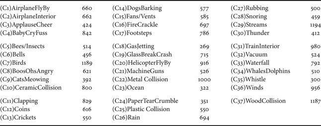
One major problem in the ESR field is the lack of a universal database. There are some consolidated acoustic databases for specific applications such as study of elephant calls [45] and acoustic for emotion stimuli [46] database. However, these databases consists of sounds either limited to an application or not directly related to environmental sounds. Papers in this field generally present their results with their own dataset consisting of an arbitrary number of environmental sound classes collected from various sources, mostly from the Internet. In the absence of a standard database, it is difficult to conduct a quantitative comparison of various approaches. Baseline classifiers with Mel-Frequency Cepstral Coefficients (MFCC) are often used to benchmark the performance of a new algorithm. However, due to significant differences in datasets of any two papers, such a performance benchmarking is futile. Hence, we built our own ESD from various sources. Most of our audio clips came from sound-effects library provided by Audio Network [47]. We also used the BBC Sound Effects Library [48], the Real World Computing Partnership's (RWCP) non-speech database [49], and freely available audio clips from various sources on the Internet [50–52]. Our database consists of 37 classes which are a mixture of sound events and ambiance sounds. Table 1 shows these classes and the corresponding number of data points sampled from all the ESR audio clips. Here, we are showing the number of sampled data points instead of the total duration of clips in the database because this gives a more insightful view of the database. All audio clips were first down-sampled to 16 KHz, 16-bit mono audio clips. These clips were then sampled to give data points for training and testing. Ideally, we wanted to have a single train/test data point to be of 6 s. However, some events are short-lived, like those from the RWCP database (metal collision, wood collision, etc.). Hence, variable length sampling was used and it resulted in data points of 0.5–6 s in length. Naturally, the number of sampled data points in ESD gives a more comprehensive view about the database in such a scenario.

Table 1. Environmental Sound Database (ESD).

B) Experimental setup

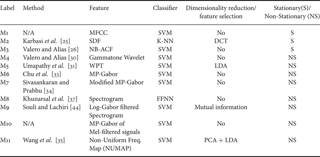
Performance comparison was made between ten selected methods listed in Table 2. Methods M1 uses sub-framing based processing scheme (see Section II) wherein averaged MFCC features from all the sub-frames are used to represent a single data point. GMM and SVM were both used for multi-class classification, and with initial trials we notice that SVM performance better than GMM, so SVM was eventually used for comparison purposes. Methods M2–M9 are selected from various publications discussed before in Sections III and IV. Method M10 is a modified method inspired from [33,34]. MP-Gabor [33] features do a sparse sampling of scale–frequency plane to extract important frequency and scale information. Modified MP-Gabor [34] tries to do better sampling of the scale–frequency plane by allocating more atoms to high-energy regions. However, this method still extracts few top atoms. One simple modification could be to increase the number of selected atoms. However, Chu et al. [33] showed that this does not result in significant improvement in classification accuracy.

Table 2. Selected methods for comparison.

It seems natural to extract features on frequency-based partitions of the scale–frequency plane and forcing the greedy Matching Pursuit algorithm to find stable representative atoms for each partition independent of inter-partition interference. Figure 3 shows such a feature extraction process. First, the signal is filtered through a Mel-filter bank with N bands (N = 5 used for M10). Then, MP-Gabor features [33] are extracted for each of the filtered outputs. Here, in order to limit the feature dimension, we used only the mean of frequency and scale parameters of selected atoms for classification, since the standard deviations of these parameters are not as useful as their respective means [33].

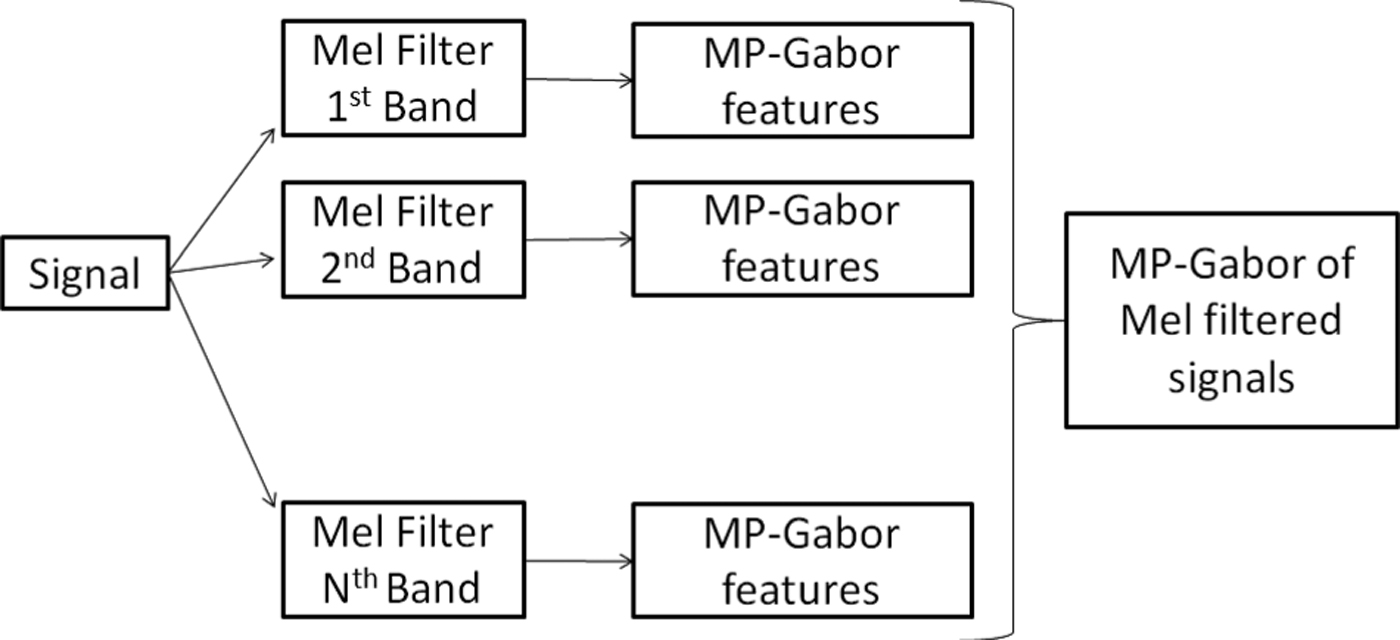
Fig. 3. The feature extraction process used in Method M10.

For all methods, we tried our best in strictly following the experimental setup as stated in original papers. However, we did have to make changes to the framework of certain methods as our database consists of variable length data-points. For example, in Method M8, authors use a sub-framing based processing scheme wherein the data from all sub-frames are concatenated to form the feature vector. Basically, this scheme assumes that the number of sub-frames is the same for all data points. For our variable length database, this is however not true. In order to comply with this requirement, we chose to replicate the data-point to form a 6 s length data-point and used an appropriate tap-sized moving average filter to smooth the overlapping regions of replicates. Similar adjustments were made in other experimental setups to fit our database. We show the pertinent details of these methods in Table 2.

We see from Table 1 that the database is non-uniform. In order to bring a sense of uniformity among various classes, we randomly selected a maximum of 400 samples to represent each class. Approximately 70% of the these samples were used for training while the remaining 30% were used for testing. To obtain reliable results, we repeated the experiments 30 times by randomly reselecting up to 400 data points for each class, and again randomly generating training and testing sets for these 400 data points. Note that some classes such as CatsMeowing(C9) and GasJetting(C18) have less than 400 samples to begin with and hence all data points are used for all trials without any sampling. We did not want to create bias by generating 400 samples by sampling with replacement. For each set of experiments, we used 5-fold cross-validation to select classifier parameters. We used MATLAB's in-built routines for GMM and FFNN, and LIBSVM [53] for SVM.

C) Results and discussion

In order to obtain stable results, we did 30 trials of training and testing as described in Section B. Classification accuracy for class CN (N = 1,2,…,37) is defined as the percentage of test data samples of class CN correctly classified. Average of the classification accuracies of all classes is used as a metric for single trial. This is done to avoid overshadowing classification accuracies of classes with less than 400 samples. Finally, classification accuracies of all trials is averaged to quantify the performance of a single method. Figure 4 shows this averaged overall classification accuracy over 30 trials.

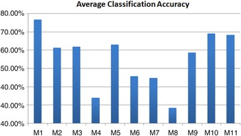
Fig. 4. Averaged classification accuracies over 30 trials.

The best classification accuracy of 76.74% is achieved M1, a stationary method. Another recent non-stationary The proposed non-stationary method M10 gives second best performance with average classification accuracy of 69.1%.method M11 gives performance close to M10, with average classification accuracy of 68.34%. Remaining two stationary methods – M2 and M3, and two non-stationary methods – M5 and M6, all give comparable performances. Surprisingly, M4, M6, M7, and M8 despite being complex features, give poor performance. Figure 5 shows the average classification accuracy over all trials. It is clear that even when single instantiations are considered, M1 performs best, followed by M10 and M11.

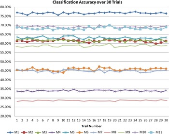
Fig. 5. Classification accuracies for 30 trials.

We performed two popular tests to verify the statistical significance of classification results. Consider to methods A and B, such that n _ab denotes number of samples misclassified by both A and B, n _{ab ^′} denotes number of samples misclassified by only A, n _{a ^′ b} denotes number of samples misclassified by only B, and n _{a ^′ b ^′} denotes number of samples correctly classified by both A and B. Let n = n _ab  + n _{ab ^′}  + n _{a ^′ b}  + n _{a ^′ b ^′} be the total number of samples in the test set. Also consider the null hypothesis that the two methods have same error rate. Given, this setting, McNemar's test statistic M _stat shown below, approximately follows a χ²-distribution with 1 degree of freedom:

(19) $$M_{stat}={{\lpar {\vert n_{ab'}-n_{a'b}\vert }-1\rpar ^2}\over{n_{ab'}+n_{a'b}}}.$$

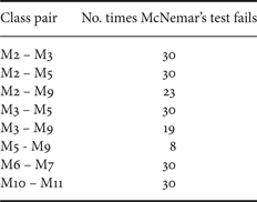
Thus, for a p-value of 0.0001, null hypothesis is rejected if M _stat is greater than χ² _1,0.9999 = 15.1367. It should be noted that McNemar's test can only be performed for one trial. Thus, with 30 trials, we get 30 different M _stat for each pair (A,B). Table 3 shows McNemar's test statistic for all pairs, and Table 4 shows pairs which frequently fail the test over 30 trials.

Table 3. McNemar's test statistic for 1 of 30 trials

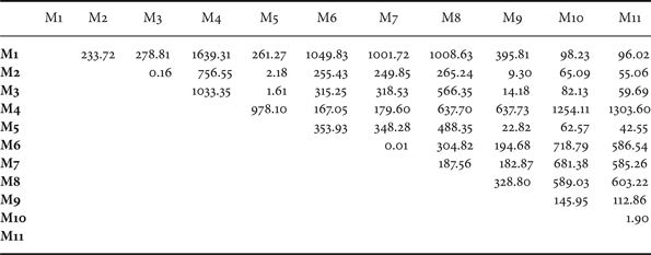
Table 4. Class-pairs that frequently failed McNemar's Test over 30 trials

The other test we performed was the paired t-test. With this test, we aim to evaluate statistical significance of classification results over all the 30 trials [54]. In fact, the choice of 30 trials was motivated by the fact that at least 20 trials are necessary for this test. In the same setting as before, let e ⁱ _A  = (n ⁱ _{ab ^′}  + n ⁱ _{a ^′ b} )/n ⁱ and e ⁱ _B  = (n ⁱ _{ab ^′}  = n ⁱ _{a ^′ b} )/n ⁱ be the error rates for ith trial, then the difference between the two error rates over all trials follow Student's t-distribution with n − 1 degrees of freedom. The T _stat for this test can be given by:

(20) $$T_{stat}={{\bar{e}\sqrt{n}}\over{\sqrt{{\sum^n_{i=1}{\lpar e^i-\bar{-}\rpar ^2}}\over{n-1}}}}$$

where e ⁱ  = e ⁱ _A  − e ⁱ _B , and $\bar{e}={1\over n}\sum^{n}_{i=1}{e^{i}}$ . Thus, with p-value of 0.0001 for a two tailed test, the null hypothesis can be rejected if absolute value of T _stat is greater than t _29,0.99995 = 4.5305. Table 5 sows the t-statistic for each pair of classes for 30 trails.

Table 5. Paired t-test statistic for 30 trials

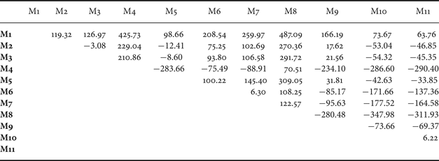
Figure 6 shows the performance comparison between the three methods – M6, M7, and M10, all based on the MP-Gabor features. Performance improvement by the proposed M10 scheme is clear in this figure. M10 gives higher classification accuracy for all classes, except C20 as shown in Table 1. The modified MP-Gabor feature [34] does not perform better than the MP-Gabor feature in [33] in most classes, except for classes like bells(C6), footsteps(C17), where sounds are clearly band limited. This is attributed to that the modified MP-Gabor feature [34] allows higher resolution in high-energy bands. From both Tables 3 and 5 it can be confirmed that the improvement of M10 over M6 and M7 is statistically significant.

Fig. 6. Comparison of averaged classification accuracies of M6, M7, and M10.

Figure 7 facilitates the comparison between the four methods – M2, M3, M5, and M9 all of which have similar performance. Non-stationary methods M5 gives a slightly better performance than the others. The two non-stationary methods, M5 and M9 are strikingly balanced with respect to their favored class-wise performances. All the classes can be divided into two distinct balanced groups where one outperforms the other by a considerable margin. However, it should be pointed out that there seem to be some characteristically definable common denominator to these two groups. For example, if we consider impact sounds from RWCP database, M5 performs better for ceramic collision (C10) and wood collision (C37), whereas M9 performs better for metal collision (C22) and plastic collision (C25). C22 and C25 sounds are sharper than those of C10 and C37. It seems only natural that log filtered spectrograms would have reasonable resolution even at higher frequencies. When M2 and M3 are compared, it can be seen that M2 performs better than M3 for more than 70% of the classes, still overall accuracy of both is comparable. This is because M2 performs really poorly for most of RWCP classes which are short-burst sounds. For these same classes, M3 gives a very good performance. Hence, we can again consider these two features as complementary to each other. Despite all these subtle differences, the results of all these four classes are not statistically different. In other words, the null hypothesis that these methods have similar average performance cannot be rejected, specifically using McNemar's test as shown in Tables 3 and 4. It is interesting to see that the test fails very often for 30 trials. t-test, on the other hand, suggests that only M2 and M3 have statistically similar results. However, it should be noted that assumptions underlying t-test do not always hold true, and it is very susceptible to Type I error [54].

Fig. 7. Comparison of averaged classification accuracies of M2, M3, M5, and M9.

Finally, we would also like to compare the performance of top three methods – M1, M10, and M11. Class-wise performance for these three methods is shown in Fig. 8. M10 and M11 give comparable performances, which is also confirmed by McNemar's test. M1 consistently performs better than M10 and M11, for both stationary and non-stationary sounds, except for few classes like birds (C7), helicopter-fly-by (C20), and thunder (C30). This leads us to conclude that simple yet powerful feature, MFCC, despite being a stationary feature, can handle even non-stationary classes better as compared to advanced (in terms of complexity) time–frequency features. However, the overall classification accuracy is still in late 1970s and hence, this leaves room for development of better features.

Fig. 8. Comparison of averaged classification accuracies of M1, M10, and M11.

It is worthwhile to point out that both spectrogram-based methods perform poorly. M8 uses the spectrogram as features directly, whereas M9 uses the spectrogram after filtering it through the log-Gabor filter bank. Both methods seem to be plagued by the curse of dimensionality. However, performance of M9 significantly improves after dimensionality reduction. The same cannot be applied to M8 as this beats the authors; original motivation of directly entire spectrogram.

VI. CONCLUSIONS AND FUTURE WORK

We conducted an in-depth survey on recent developments in the ESR field in this paper. Existing ESR methods can be categorized into two types: stationary and non-stationary techniques. The stationary ESR techniques are dominated by spectral features. Although these features are easy to compute, there are limitations in the modeling of non-stationary sounds. The non-stationary ESR techniques obtain features derived from the wavelet transform, the sparse representation and the spectrogram.

We performed experimental comparison of multiple methods to gain more insights. Stationary feature MFCC gives best performance followed by the proposed non-stationary features in M10, and recently proposed non-stationary features M11, i.e. NUMAP [35]. Other than this, the performance of stationary and non-stationary methods is, at best, comparable. The wavelet-based method gave results comparable to stationary methods such as SDF and NB-ACF. In contrast, spectrogram based methods perform poorly. We believe there is a need for a better feature selection process and a dimensionality reduction process to simplify the spectrogram features. Although these features contain most detailed information about audio clips, they fail to translate this information into meaningful models.

Finally, we would like to point out two future research and development directions.

• • Database Expansion and Performance Benchmarking

  We need to increase the database to include more sound events. Also, there are numerous kinds of environmental sounds yet there is no standard taxonomy for them. Potamitis and Ganchev [21] made an effort to classify sounds to various categories from the application perspective. However, this problem is far from completion.

• • Ensemble-based ESR

  A set of features with simplicity of stationary methods and accuracy of non-stationary methods is still a puzzle piece. Moreover, considering the numerous types of environmental sounds, it is difficult to fathom a single set of features suitable for all sounds. Another problem with using a single set of features is that different features need different processing schemes, and hence several meaningful combination of features, which would be otherwise functionally complementary to each other, are incompatible in practice. This school of thought, and success stories of [55–57] directly lead us to ensemble learning methods. Instead of learning/training a classifier for a single set of features, we may use multiple classifiers (experts) targeting different aspects of signal characteristics with a set of complementary features. Unfortunately, there is no best way to design an ensemble framework, and a considerable amount of effort is still needed in this area.