Wealth and Weight: The Impact of the BMI According to Income in European Countries

Abstract

This study analyses the evolution of body mass index (BMI) as income increases across the population, controlling for age, sex, educational level, marital status and some lifestyle habits. To this end, a quantile regression, an econometric technique that readjusts the weights of the variables in each quantile to minimize deviations, has been carried out, where the variable that orders the sample is income. We use 316,777 observations from the European Health Interview Survey (EHIS) for these regressions. This approach allows us to separate the regression analyses for low-, middle-, and high-income groups, evidence that as individual income increases, BMI tends to rise. Consequently, individuals with higher incomes exhibit higher BMI levels. Additionally, the estimated parameters for explanatory variables increase with income, signifying that wealthier individuals not only have a greater likelihood of increased BMI but also that socio-economic factors influencing BMI – whether positively or negatively – evince a stronger impact as income levels rise.

Introduction

There has been growing concern about physical health in developed countries in recent decades, especially with regard to obesity, as Livingstone (2001), Hursting and Dunlap (2012), Meurling et al. (2019), Okobi et al. (2021), Ali et al. (2022) or Griffith (2022) rightly point out. At the same time, there is an observable upward trend in the prices of typically healthy foods, making it cheaper for consumers to choose fast food options, such as burgers and other processed items, over preparing meals with fish, fruits, or vegetables. The rising cost of healthy diets has been widely documented by various authors, including Williams (2007) and, more recently, Daniel (2020), who notes that consumers often determine whether food is cheap or expensive by comparing it with similar options. As a result, healthy foods are generally perceived as more costly and, thus, less appealing. Furthermore, households with limited budgets face significant constraints due to food prices, both in real terms of purchasing power and, as Haws et al. (2017) suggest, due to a societal belief that healthy foods are more expensive, even if this is not always the case. Additionally, the recent report ‘The State of Food Security and Nutrition in the World 2024’ from the Food and Agriculture Organization of the United Nations (FAO) underscores the rising cost of maintaining a healthy diet. In this context, this study analyses whether an individual’s position in the income quartile distribution influences the relationship between a set of key determinants and the body mass index (BMI) of the individual.

Economic literature has paid special attention to the relationship between income and BMI, but there is still no consensus on the effect of income on BMI. Thus, Monteiro et al. (2001) showed, for societies in transition, that income tends to be a risk factor for obesity. Similarly, Schmeiser (2009) argues that income increases BMI and the likelihood of obesity in women with wage earnings, so that as household income increases so does the risk of obesity problems for women. Masood and Reidpath (2017), in a comparative study of 70 countries, report that BMI increases with increasing Gross National Income in purchasing power parity. On the other hand, Chang and Lauderdale (2005) show for the United States that obesity has increased at all income levels.

However, there are authors who show the opposite, i.e. that income exerts a BMI-reducing effect. Jolliffe (2011), for example, argues that increases in income are correlated with healthier BMI values. In the same vein, Kpelitse et al. (2014) show, in a study for Canada, that increases in household income tend to reduce weight in both men and women. Indeed, as Oliver and Hayes (2008) show, living in poorer neighbourhoods is associated with higher BMIs.

For Europe, we find similar results to those described above, i.e. economic literature points to a negative relationship between income and BMI. Thus, Lakerveld et al. (2015) state that residents in low-income neighbourhoods eat less fruit and vegetables and drink more sugary drinks, thus having a higher BMI. Even so, authors such as Roskam et al. (2010) qualify that there is a direct relationship between income and obesity, although only in the less educated male population. For their part, Salmasi and Celidoni (2017) state that poor individuals are more likely to be obese than non-poor individuals. In any case, work for Europe has focused on explaining the causes of this apparent negative relationship between income and BMI. Thus, Brunello and d’Hombres (2007) show that an increase in average BMI reduces the real earnings of men and women, i.e., income would not be the cause of higher BMI but a consequence. The same conclusion is reached by Villar and Quintana-Domeque (2009), who argue that the negative relationship between household income and BMI for women is due to the fact that obese women are ‘penalized’ by the labour market.

More recent work stresses the idea that being overweight increases with income only in poorer countries and population groups, while in richer countries, the relationship is negative (Ameye and Swinnen 2019). However, other authors such as Talukdar et al. (2020) argue that the prevalence of obesity in the population shows a positive relationship with national income and there is no evidence that the relationship, although weakening, becomes negative at higher income levels (‘weight Kuznets curve’).

Consequently, firm conclusions regarding the relationship between income and BMI remain elusive. Thus, the primary aim of this article is to explore how income influences the mediation of socio-economic determinants of high BMI. To achieve this, the analysis controls for multiple variables understood to be key factors affecting BMI aside from income (age, male, marital status, living in an urban environment, educational level, sport, smoking, alcohol consumption, and fruit and vegetable consumption). After empirical analysis, we find evidence to support that our hypothesis holds in European countries: individuals with higher income levels are statistically more likely to present higher weight than their lower income counterparts. In addition, thanks to quantile regression, it is identified that the estimated parameters of the control variables increase as the regression is placed in higher quintiles, in other words, those variables that control the regression by virtue of physical inactivity, social context and lifestyle habits have higher results in absolute value and with greater significance on BMI.

The method used is described here, starting with an explanation of the analysis technique to be used (quantile regression), as well as the nature of the data used, the model to be estimated and ending with the presentation of the results and discussion of these results. After completing the empirical analysis, the limitations of the empirical analysis are presented, which will be the basis for closing this research with the conclusions drawn from it.

Method

Estimation Technique

The technique on which the following analysis is based is called quantile regression, building upon the previous work of Amate-Fortes et al. (2024). The objective of quantile regression is the same as OLS regression, i.e. to model the relationship between the variables under analysis. However, the advantage of this technique lies in the possibility of estimating different regression lines for different quartiles of the endogenous variable. The variable that will divide the data into different quartiles is the income level, allowing for regressions to be obtained for three distinct quartiles. These quartiles are θ = 0.25, which will include data from individuals with the lowest income levels; θ = 0.5, which will represent individuals with middle income levels; and θ = 0.75, which will capture information from individuals with the highest income levels. Thus, the model specification is presented in equation (1):

(1) $${Y_i} = {X_{i\;}}{\beta _\theta } + {u_{\theta i}}$$

where, ${Y_i}\;$ is the endogenous variable, ${X_{i\;}}\;$ represents the matrix of exogenous variables, ${\beta _\theta }$ is the parameter to estimate corresponding to the quantile $\theta $ and ${u_{\theta i}}\;$ is the random disturbance corresponding to the quantile $\theta $ . Analogous to the OLS estimation technique, which states that $E\left( {{y_i}|{x_i}} \right) = {X_{i\;}}{\hat \beta _{{\rm{OLS}}}}$ and hence that $E\left( {{u_i}|{X_i}} \right)=0$ , in quantile regression it is assumed that ${\rm{Quan}}{{\rm{t}}_\theta }\left( {{y_i}|{x_i}} \right) = {X_{i\;}}{\beta _\theta }$ which implies that ${\rm{Quan}}{{\rm{t}}_\theta }\left( {{u_{\theta i}}|{x_i}} \right)=0,\;$ this being the only assumption made about the random disturbance in this technique. In parallel to the way quantile regression is approached from the OLS technique, its problem can be posed from the same technique. After its development, the expression for parameter estimation in quantile regression is expressed as in equation (2):

(2) $${\rm{Min}}\;{\beta _\theta } \in \mathbb{R}\;\;\left[ {\mathop \sum \nolimits_{{Y_i} \geq {X_{i{\beta _\theta }\;}}} \theta \left| {{Y_i} - {X_{i\;}}{\beta _\theta }} \right| + \mathop \sum \nolimits_{{Y_i} \geq {X_{i{\beta _\theta }\;}}} \left( {1 - \theta } \right)\left| {{Y_i} - {X_{i\;}}{\beta _\theta }} \right|} \right]$$

Equation (2) shows how the objective is to minimize the absolute deviations weighted with asymmetric weights, i.e. each deviation corresponding to observation i is given a different weight in the regression depending on the quantile whose regression line is being estimated. In addition, the advantage of approaching the optimization problem in this way is that, by using absolute values instead of square deviations, if outliers are present, the estimation is not altered as much. This improvement comes from the fact that in this model the errors are considered linearly, whereas with other techniques such as OLS, by squaring the errors, the importance of the outliers is increased, which subsequently increases the errors quadratically.

Data

All data used in this research are obtained from The European Health Interview Survey (EHIS). This study utilizes the second wave of the European Health Interview Survey, conducted between 2013 and 2015 across all EU countries, Iceland, and Norway. Data collection for EHIS-2 took place in 2013 for Belgium and the United Kingdom, in 2014 for Bulgaria, Czechia, Estonia, Greece, Spain, France, Croatia, Italy, Cyprus, Latvia, Lithuania, Luxembourg, Hungary, Malta, the Netherlands, Austria, Poland, Portugal, Romania, Slovenia, Slovakia, Finland, and Sweden, and in 2015 for Denmark, Germany, Ireland, Italy, Iceland, and Norway to ensure data consistency. Wave 2 data were chosen over Wave 3, as the latter were collected during a period impacted by the COVID-19 pandemic in certain countries, such as Albania, Germany and Malta. This database contains information on European residents aged 15 and over, divided into four modules: health status, health care use, health determinants and socio-economic background. That said, descriptive statistics for each quantile of the following variables are given in Tables 1, 2, 3 and 4. Finally, no weighting was applied to the data.

Table 1. Descriptive statistics for the first quartile (Q₁).

Table 2. Descriptive statistics for the second quartile (Q₂).

Note: All data provided are unweighted averages.

Table 3. Descriptive statistics for the third quartile (Q₃).

Table 4. Descriptive statistics for the maximum values.

Note: All data provided are unweighted averages.

The dependent variable is body mass index. This variable is not directly available in the EHIS, but it does contain height and weight. Based on these variables, by dividing weight in kilograms by the square of height in metres we obtained the variable. With this variable, we aim to analyse whether there is a positive correlation between purchasing power and to have higher weight within the population.

The income variable is not among the variables in the equation to be estimated, but it is present, since it is the variable that orders the sample in our quantile regression, so that we will have results from three estimates: one for low income, one for middle class and one for high income. It is important to note that while individual income amounts are not directly available, we utilize income quartiles derived from the income distribution within each respondent’s country of residence. This approach allows us to categorize individuals into relative income groups (low, middle, and high) based on their position within the national income distribution.

The independent variables will control various dimensions that affect an individual’s BMI, in order to discount these effects and obtain the direct relationship between BMI and income. The first dimension that has been covered is the age of the individual, which is captured by instrumental variables that cover different age intervals, these being: age15–24, age25–34, age35–44, age45–54, age55–64, age65–74, age75–84 and age85 (85 or more). Of these, ‘age15–24’ will be omitted from the model to avoid errors in the model. Then, all ‘age (range)’ variables should be interpreted in relation to the youngest age segment. In addition, to make certain physical constraints more concrete, we have the variable ‘Male’ which takes a value of 1 if the respondent is male and 0 otherwise.

To contextualize the respondent in their social environment, we have added the variables ‘Spouse’ which will take value 1 in the case of being married and 0 otherwise, ‘URBANzone’ which will take value 1 in the case of living in an urban area and 0 otherwise, and ‘EducGlobal’ which will indicate the educational level of the respondent, this variable taking values 0 (nursery school); 1 (primary education); 2 (secondary education); 3 (upper secondary education); 4 (higher than secondary but not tertiary); 5 (short-cycle tertiary education); 6 (university degree or equivalent); 7 (university master’s degree) and 8 (doctorate).

Lifestyle is approximated by the following four variables that capture healthy or unhealthy lifestyle habits. ‘CardioDays’ takes values between 0 and 7, being the number of days per week in which the individual performs physical activities that cause at least a small increase in breathing or heart rate for at least 10 minutes continuously. Similarly, ‘FrecALGlobal’ captures the number of days per week on which the individual consumes alcoholic beverages. ‘Ncigar’ counts the number of cigarettes the individual consumes per week and ‘UnitsFrutVeg’ counts the number of units of fruit and vegetables the individual consumes in a typical week.

Model

The linear model is made up of the variables discussed previously, with data and the methodology also previously discussed. The following equation will be estimated for each of the three quartiles in order to be able to establish comparisons between the different income levels. This is the reason why a selection of different variables is not made for each income level, assuming the limitation that each income level has different determinants. With all this, equation (3) offers the most significant results among all the combinations of variables in the EHIS.

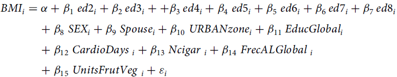(3) $$\begin{gathered}BM{I_i} = \alpha + {\beta _1}\;ed{2_i} + {\beta _{2\;}}ed{3_i} + + {\beta_{3\;}}ed{4_i} + {\beta _4}\;ed{5_i} + {\beta _5}\;ed{6_i} + {\beta _{6\;}}ed{7_i} + {\beta _{7\;}}ed{8_i} \\ + {\beta _8}\;SE{X_i} + {\beta _9}\;Spous{e_i} + {\beta _{10}}\;URBANzon{e_i} + {\beta _{11\;}}EducGloba{l_i} \\ \!\!\!\!\!\!\!\!\!\!\!\!\!\!\!\!\!\!\!+ {\beta _{12}}\;CardioDays{\;_i} + {\beta _{13}}\;Ncigar{\;_i} + {\beta _{14}}\;FrecALGlobal{\;_i} \\ \!\!\!\!\!\!\!\!\!\!\!\!\!\!\!\!\!\!\!\!\!\!\!\!\!\!\!\!\!\!\!\!\!\!\!\!\!\!\!\!\!\!\!\!\!\!\!\!\!\!\!\!\!\!\!\!\!\!\!\!\!\!\!\!\!\!\!\!\!\!\!\!\!\!\!\!\!\!\!\!\!\!\!\!\!\!\!\!\!\!\!\!\!\!\!\!\!\!\!+{\beta _{15}}\;UnitsFrutVeg{\;_i} + {\varepsilon _i} \\ \end{gathered}$$

Results and Discussion

All the information from the regression is shown in Table 5. Most of the coefficients are highly significant and consistent with what could be expected a priori for each variable. Perhaps the low coefficient of determination obtained stands out; however, this is not, a priori, a drawback since our model is for analytical purposes and not for forecasting. The coefficient of determination will be explained in depth at the end of this section once the coefficients of all the variables in the model have been presented. In addition, the coefficient of determination highlights the omission of relevant variables, which is one of the limitations of our research – the non-availability of the desirable data for everyone. The limitations will be discussed at the end of this section.

Table 5. Estimation results for each quartile of income.

Note: * Significant at 10%; ** significant at 5%; *** significant at 1%.

Figure 1 presents the conditional density functions of BMI for each age group by income quartiles. These provide valuable preliminary insights that help to contextualize the results prior to conducting econometric regression analysis. First, the figures reveal that BMI density varies significantly with age. Younger individuals (particularly those aged 15–24) tend to cluster towards the left, indicating lower BMI values.

Figure 1. Conditional density functions of BMI for each age group of the population distributed by the income quartile

Second, as income quartiles increase, particularly at the extremes, dispersion decreases, suggesting greater heterogeneity in BMI across age groups within the lower income quartiles. This pattern changes in the density functions for higher income levels, where, despite some dispersion, the functions tend to overlap, indicating convergence.

Third, a rightward shift is observed in some age groups as we move to higher income quartiles, which could suggest a correlation between higher income levels and higher BMI values. Lastly, the differences between income levels are more pronounced among younger groups, while for older groups, such differences diminish. This implies that for older individuals, income level is less significant in determining BMI.

With respect to the econometric analysis, answering the question that gave rise to this research, we seem to find evidence that higher income levels are associated with higher BMI values. This observation arises from the fact that the coefficients of the intercepts are increasing when controlling for the physical, social and lifestyle dimensions of the individual. Furthermore, it is also observed that the coefficients of most variables become larger in absolute value as we move to a higher quartile; consequently, it is assumed that the same factor has a greater impact on BMI, i.e. people with higher incomes are more exposed to changes in the stimuli collected in the variables. Thus, if we consider two subjects of the same age, statistically the one with a higher income level will have a higher BMI, ceteris paribus.

Once this observation has been made, let us specify how the control variables of the model behave.

First, the variables capturing age (Age25–34, …, Age85) should be interpreted considering that Age15–24 is omitted. Therefore, these coefficients are in relation to Age15–24, i.e. they are interpreted comparatively with respect to the youngest age group. From the age variables it is interesting to see how the coefficient associated with the same age group for a higher income level is higher, i.e. in the case of two individuals of the same age, the one with a higher income will report a greater BMI. Likewise, a positive association is observed between age and reported BMI, with higher BMI values generally associated with older age across income levels. For example, a 60-year-old is likely to have a higher BMI than a 40-year-old, and a 40-year-old is likely to have a higher BMI than younger individuals. This observation has been supported in previous studies such as Okati-Aliabad et al. (2022), who concluded that the prevalence of obesity increases with age. Furthermore, according to Knapp et al. (2022) the recent global pandemic caused by COVID-19 has led to a significant increase in BMI in the population, which may critically affect public health and health equity. This trend is reversed from age 75 onwards, as shown by the Age75–84 variable, which has a lower coefficient than the previous age variable for the first time, so we can conclude that after 75 years of age people begin to lose weight involuntarily. This happens, according to studies such as Seidell and Visscher (2000), Moriguti et al. (2001), Chapman (2011) or more recently Díez-Villanueva et al. (2022) and Senee et al. (2022) because at this age there is usually a decrease in caloric intake due to the onset of numerous diseases that affect eating patterns, such as coronary heart disease, atherosclerosis, type 2 diabetes or hypertension, deficiency or Alzheimer’s disease and other medical situations. Therefore, it can be concluded for all these variables that having greater income does increase the likelihood of presenting a higher body weight, and, moreover, this event worsens with age.

With respect to the MALE variable, we can conclude that for low and intermediate income levels, male individuals are more likely to present a higher weight than female individuals, this could be due to the fact that, as Ålgars et al. (2009) and more recently Quittkat et al. (2019) state, female individuals generally feel less satisfied with their bodies than male individuals, therefore, they take more care of their image and diet, causing male individuals to have comparatively higher levels of body mass index. This pattern shifts at higher income levels, where BMI values for both sexes appear to converge. Female individuals show a weaker association between income and higher BMI. Specifically, the coefficient decreases from 1.92 at lower income levels to 0.9 at higher levels. Consequently, the influence of the male variable is practically halved, indicating a certain degree of convergence between sexes as income levels rise, since the coefficient progressively diminishes.

Turning to variables defining social context, SPOUSE indicates that those living in couples are slightly more likely to exhibit higher body mass index values compared with those living alone, as noted by Gneezy and Shafrin (2009), an observation supported by Lee et al. (2020) who observed within their sample of 137,608 participants that married people showed a higher BMI than those with other marital statuses. However, as with the MALE variable, when we consider how this variable is affected by higher levels of income, we see that its effect diminishes. Therefore, a married couple with high purchasing power will be less likely to have a higher BMI than a married couple with lower purchasing power, this fact could be due to the access to surgeries and services focused on personal care or a better diet according to the assumptions described above by Daniel (2020) and others.

URBANzone is only significant for intermediate income levels. This does not imply that its presence does not contribute anything to the estimation for low- and high-income levels, since it is convenient to control where the population lives to improve the explanatory power of the other variables in the model. With respect to the significant coefficient for intermediate income, it is negative although derisory. It shows that people living in urban areas are slightly more likely to exhibit lower BMI values compared with those living in rural environments, which could be explained by the lifestyle in cities where the population is more active. These results support Zhao and Kaestner’s (2010) finding that there is a negative association between population density and weight of the individual.

With respect to EducGlobal we see that this is significant only for respondents with middle- and higher-income levels. This could be because, among lower income levels, there are no significant differences in educational attainment and therefore the variable has no explanatory power. On the other hand, when considering the regressions for the other quartiles, both are negatively related to BMI, although with a greater influence on higher incomes. Similarly, it can be observed that individuals with higher levels of education appear to exhibit lower BMI levels, as highlighted by preliminary studies such as those conducted by Marques-Vidal et al. (2010) and Lopez-Arana et al. (2013). More recently, Wang et al. (2021) and Yang et al. (2021) found that those individuals with higher levels of education have a persistently lower BMI level than their less educated counterparts.

Entering the block of variables that try to approximate lifestyle habits; generally, all of them offer similar conclusions to those traditionally established by medicine and which are generally known. Likewise, before delving into a detailed description of each variable individually, the results show that all these variables amplify their effect as we move from the lowest income quartile to the middle-income quartile, and finally to the highest income quartile, as the estimated coefficients increase. Having clarified the general trend in lifestyle habits, let us look at each variable individually.

The first variable in this category is CardioDays, which shows that the more days of physical activity, the lower the BMI the individual will have according to studies such as Lopes et al. (2019), Chen et al. (2023) and Rao et al. (2023). Ncigar shows positive results, but these are close to zero. Therefore, we conclude that smoking may only be slightly associated with higher BMI values, despite the fact that statistically significant coefficients are observed at all three levels. Although it is true that our coefficient does not yield major conclusions, it could reaffirm the conclusions of Munafò et al (2009) where they concluded that ex-smokers tend to increase their BMI by 1.6 kg/m² with respect to those who have never smokeds. The FrecALGlobal variable shows a priori unexpected results, since, in principle, one might think that alcohol consumption decreases BMI because the coefficients are significant and negative. However, this relationship could be due to an endogeneity issue between alcohol consumption and BMI, as Kleiner et al. (2004) attest. These authors found an inverse and significant relationship between alcohol consumption and BMI, which is due to the fact that more obese patients consume less alcohol. They also state that, in the later years of their study, those female individuals who increased their BMI progressively reduced their alcohol consumption. This relationship, as we can see, intensifies as the individual has a higher level of purchasing power. Finally, with respect to UnitsFrutVeg, we see that it is not significant for individuals with a lower level of purchasing power; this could be due to the fact that the amount of fruit and vegetables consumed at these income levels is negligible and therefore this variable has no explanatory capacity for low-income levels. On the other hand, we see that its significance increases a little for middle incomes and finally it has the maximum significance for high incomes. Therefore, we understand that the explanatory power of this variable increases with income. This phenomenon may be attributed to the fact that the descriptive statistics for the variable capturing fruit and vegetable consumption indicate a higher mean for the upper quartiles, with the maximum value also being greater among those with higher income levels. However, it is not a result of significant importance. It also seems to be found that fruit and vegetable consumption is associated with a higher level of BMI. In this regard, it is worth noting the analysis of Field et al. (2003), where they conclude that while the recommendation to consume fruit and vegetables may be well founded, there is no evidence to support beneficial effects of fruit and vegetable consumption on weight regulation in individuals. Likewise, Azagba and Sharaf (2012) showed through quantile regressions that the effects of fruit and vegetable consumption on body mass index were not uniform, i.e. depending on the BMI distribution of the individual, the outcome of consuming fruit and vegetables may vary. Finally, to close the explanation of fruit and vegetable consumption, it could be explained that the intercept suggests a positive correlation between fruit and vegetable consumption and higher BMI, likely reflecting that individuals with higher incomes tend to consume more of these foods and also exhibit higher BMI values, as indicated by the highest intercept, without implying a causal relationship. In this way, two variables with a positive trend in relation to the increase in income would be related, and it could be a spurious relationship like the well-known case of storks and the birth of babies discussed in works such as that of Höfer et al. (2004).

Finally, before reaching the conclusions, the different coefficients of the model were graphically represented with their values for each quantile point (expressed by the dark grey line) with their respective confidence intervals (represented by the light grey shading), which are shown in Figure 2. Here, we can see how the intercept explaining the relationship between BMI and income level increases progressively, which undoubtedly indicates that higher income levels imply higher levels of BMI, considering that the effects of all other variables are controlled for. Furthermore, these representations reaffirm the statistical results explained above based on the data obtained from the model shown in Table 5.

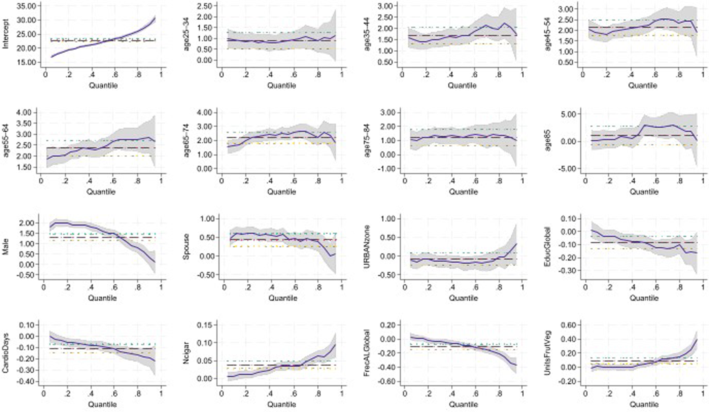
Figure 2. Graphs of the quantile regression coefficients.

In conclusion, with all the variables developed, we can point out that the variables increase in significance and the absolute value of the coefficients as the level of income increases. In addition, based on the intercept, the higher the income of the individuals, the higher the BMI value obtained. Therefore, it would not be unreasonable to assume that higher income levels are positively associated with higher BMI and, therefore, that countries with higher incomes could have a higher prevalence of individuals with a higher BMI given the association found between income level and BMI. In addition to concluding that income is indeed contributing to weight gain, the use of quantile regression shows that the effects of the variables are amplified by income. Thus, among the higher income population there is a major disjuncture in terms of their BMI, since for this population the variables that favour a decrease in their BMI (living in urban areas, practising sport, etc.) have a greater effect on them than on their lower income peers, just as the effects of the variables that tend to increase their BMI (age, male, marital status, smoking, etc.) are also intensified. This polarization of BMI in the affluent population is not only represented by the increase in the coefficients as we move to higher income quartiles but is also evidenced by the coefficient of determination decreasing as we move to higher income quartiles. In other words, as the wealthier population has a greater polarization in their BMI owing to the intensified effect of the control variables, the goodness of fit of the regression for this segment of the population is worse despite the fact that quantile regression is more consistent than other econometric techniques in minimizing weighted absolute deviations.

Limitations

The main limitations of our analysis are that the data are drawn from a survey, namely the European Health Interview Survey (EHIS). This limits us in two ways: the first, and less relevant, is that we have to assume that survey responses may not be completely honest. However, given that we have 316,277 observations, we believe that the general trend captured by the results does resemble reality. The second limitation of obtaining our data from the EHIS would come from its geographical scope, in other words, the results obtained are applicable to the European population, and different results may be found in other geographical areas.

A limitation that must also be considered is that the variable used to analyse an individual’s weight is the body mass index (BMI). While it is the standard measure for addressing this type of issue, it does have its limitations. For example, individuals with a high proportion of muscle mass may obtain high BMI results without experiencing any form of being overweight; on the contrary, they may even have an ideal and above-average physical condition. However, such cases are not accounted for in this study, as the variable itself is unable to distinguish these situations. For this reason, we focus on weight in general and not on overweight in particular.

Another limitation could be that we do not have all the variables that we would like; for example, it would be interesting to have a variable that would inform us of the level of stress or anxiety of individuals, as these disorders undoubtedly have proven effects on the lifestyle and therefore the weight of individuals. In addition, being able to incorporate a dimension such as mental health into this analysis would enrich the analysis considerably. The limited number of variables in our analysis, while restricting our ability to fully account for factors influencing BMI, does not detract from the exploratory nature of our study. Our focus is on identifying correlations rather than developing predictive models.

Finally, due to the analysis we have carried out, quantile regression, in order to be able to make comparisons we must adjust to using the same variables for the different income levels. However, this in turn limits us since each income level could have different determinants. Determinants that we have not been able to address because, if we had done so, we would have different regressions for each income level and therefore we could not have made comparisons between the different quartiles.

Conclusions

The origin of this work lies in the growing concern about health and physical appearance in developed countries, especially in relation to high BMI levels, as pointed out by various authors – as discussed above. However, we ask: is it economic growth itself that generates dynamics that lead to an increase in the weight of the population? In this way, a small conflict would be generated in which the desired economic growth brings us higher levels of economic and social well-being but may be the origin of other phenomena that provoke animosity.

While the interpretation of these findings is tempered by certain limitations, it’s important to note two key points. First, the analysis does not explicitly account for country-specific factors, limiting the generalizability of the results beyond the sample countries. Second, BMI values were not standardized using country-specific cut-off points, which could influence the observed patterns. For the sake of research integrity, we have chosen to present the data in this way to avoid modifying the original information.

In order to study this hypothesis, the EHIS data have been obtained and polished and analysed through a quantile regression to differentiate the results according to the level of income of the individual with respect to the distribution of their country. According to the results obtained, we could conclude that people with higher purchasing power are those who are more exposed to the variables studied. And, therefore, those more likely to exhibit higher BMI values. This phenomenon is easily observable through the constant terms of the different quantile regressions we have performed. Because the constant term in our model represents the predicted BMI when all other variables are held constant, the 26.26% difference we observe between the highest and lowest income quartiles suggests a positive relationship between income and BMI. In other words, higher incomes tend to be associated with higher BMI levels, ceteris paribus.

On the other hand, in our analysis we have used numerous control variables that we have distributed into three categories (physical constraints, social context and lifestyle habits) to try to isolate the effect of income from other external variables. These exogenous variables, in addition to fulfilling their role as control variables, have also allowed us to reaffirm the conclusions of other studies that have studied these variables with respect to body mass index. Among all of them, especially surprising is the case of fruit and vegetable consumption, which shows a non-linear relationship with respect to BMI or, in other words, it does not have a uniform and constant relationship that relates it to body mass index, as pointed out by authors such as Field et al. (2003) and Azagba and Sharaf (2012). It has also been shown that the most relevant variables in determining an individual’s BMI are age and male, variables that are impossible to influence. However, the beneficial effect of education and sport in reducing BMI and the harm caused by bad lifestyle habits such as smoking are contrasted. These are circumstances that states can influence through their policies.

Based on the above, the novelty of this research to general knowledge on the subject lies in its strategic application of quantile regression, an econometric technique that allows us to investigate the determinants of BMI across different income levels. This method empowers us to conduct separate regressions tailored to distinct income quartiles, which are specifically ordered from lowest to highest income level. This technique allows us to perform different regressions for different quantiles, weighting each observation according to the quantile to minimize the estimation errors, so that we have really powerful results for each income level despite the fact that all the regressions share the same variables. This technique allows us to support our hypothesis and main contribution: those with higher income levels also have higher body mass index values, and therefore we can affirm that ‘There seems to be a higher prevalence of high BMI levels among individuals with higher income levels in general terms’. In addition, we have also obtained results from the numerous control variables of the model that reaffirm the results of previous studies and give visibility to issues that are being overshadowed by general knowledge. It is also shown that the variables that determine BMI, both for increasing and decreasing it, see their effect on it amplified as the population’s income increases. Therefore, it can be deduced that for higher income levels there are greater difficulties in finding a linear regression that adequately explains the variations in BMI, since in this segment there is greater diversity of values. This observation is reinforced when considering the coefficient of determination, which decreases as the quantile on which the regression is performed increases, although quantile regression minimizes the deviations by giving different weights to the variables in order to obtain the best fit.

In conclusion, based on the above and the limitations we have, it is recommended that European countries carry out public campaigns on good lifestyle habits that favour the reduction of being overweight or obesity in the people affected, For example, campaigns that favour sporting activity, as well as evidence of the CardioDays variable and other measures to promote good nutrition education, and education in general, facilitating access to education and trying to reduce the school dropout rate with the aim of benefiting the productivity of the economy as well as the health of individuals, as supported by EducGlobal. These measures will reduce the future burden of public health care spending on high-BMI-related conditions and contribute to health equity.