Introduction
Sea ice on the large scale is characterized by leads and ridges that typically have a given orientation. Because of various flaws we would expect that the ice will form oriented leads and ice-thickness characteristics that control the heat and moisture fluxes into the atmosphere. Moreover the flow of sea ice and open water created under compact ice conditions are largely controlled by these oriented weaknesses.
Present large-scale sea-ice models (e.g. Reference HiblerHibler, 1979; Reference Stössel, Lemke and OwensStössel and others, 1990; Reference Flato and HiblerFlato and Hibler, 1992; Reference Holland, Mysak, Manak and OberhuberHolland and others, 1993) are based on smooth-continuum failure criteria that do not explicitly take into account the formation of leads and cracks. Observations both on the large scale (Reference Marko and ThomsonMarko and Thompson, 1977) and in the laboratory (Reference Schulson and NickolayevSchulson and Nickolayev, 1995) indicate that the failure of ice typically takes place by fracturing, especially under divergent conditions. Also the similarity of results between different scales (Reference Schulson and HiblerSchulson and Hibler, 1991) and observations on the large scale suggest that similar mechanisms may apply if appropriate scaling can be carried out.
To describe completely this composite system would require an anisotropic model (see e.g. Reference Coon, Echert and KnokeCoon and others, 1992) with a memory of past oriented leads. However, many aspects of the fracture-based failure of sea ice may be determined by examining the response of a system beginning initially with a uniformly oriented set of weak thin-ice leads embedded in thicker ice. The principle here is that while lead formation is locally anisotropic, such a composite is isotropic in the sense that its mechanical response will be the same regardless of which direction the external stresses are applied. Also such an approach may be particularly relevant to climate studies where we are more concerned with predicting the statistical characteristics of leads rather than particular occurrences.
In this paper we present a model for the treatment of leads and oriented flaws in large-scale sea-ice models relevant to climate studies. While the theoretical framework is anisotropic in character, we here examine isotropic realizations of the model, beginning initially with uniformly oriented leads or flaws in all directions. While we do not consider how these leads were formed, we note that fractures at almost all scales are ubiquitous features in pack ice. In addition, an approximate strain-hardening extension is proposed where only oriented leads having the potential to open rapidly are allowed. Both these isotropic models yield preferential deformation along a particular set of intersecting leads with the particular deformation and "lead pair" depending on the confinement stress. The resulting yield curves and flow characteristics form two archetypal fracture-based rheologies that should have utility in current numerical investigations of climate.
Theory
The essential idea is, following Reference Coon, Echert and KnokeCoon and others (1992), to make use of oriented flaws or weak leads in thicker ice. However, rather than assume an orientation and intersection angle for leads we only assume that the thick and thin ice obey viscous-plastic constitutive laws. The anisotropic flow and yield characteristics, as well as lead orientation and intersection angles, then become part of the model predictions.
To develop the basic theory let us first consider a single weak lead embedded in thick ice. We assume, as in Figure 1, that within the plane of the ice sheet the lead goes completely through the geographical region of interest. Consider that the lead has area A and strength P′ and is embedded in thick ice of strength P and area 1 – A as shown in Figure 1. We consider that within the plane of the sheet, both the lead ice and thick ice obey an isotropic constitutive law with a yield curve described by a truncated ellipse as discussed in the Appendix. Envelopes of this kind characterize compressive failure of columnar sea ice when biaxially loaded across the columns (Reference Schulson and NickolayevSchulson and Nickolayev, 1995). For this constitutive law (see Appendix) the stress may be expressed in terms of the strain rate by the Reiner–Rivlin constitutive law (e.g. Reference HunterHunter, 1983) which for Cartesian tensors is given by:
where η, ζ and P are functions of the strain-rate invariants, repeated subscripts are summed over 1,2 and δ ij is the kronecker delta.
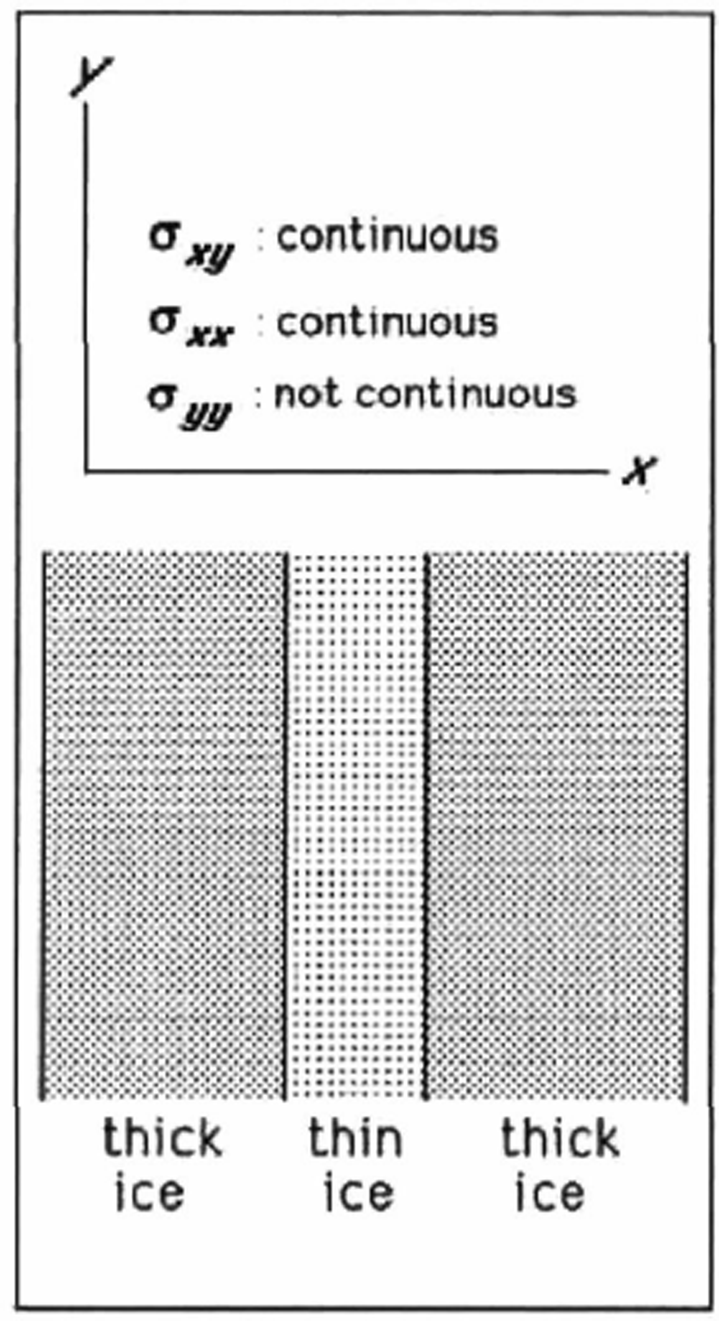
Fig. 1. Schematic view of oriented thin ice lead embedded in thick ice.
We consider a strain rate έ yy 0 with the same value in both the leads and thick ice: έ yy ′ = έ yy = έ yy 0. We now consider a strain rate έ xx 0, which is composed of έ xx ′ in the thin ice, and έ xx in the thick ice in a manner such that
and a shear-strain rate έ xy 0 such that
We insist that the stress is continuous at the thin-ice thick-ice boundary, which implies that σ xx and σ xy , the compressive and shear stresses across a face with normal in the x direction, are continuous. Using the truncated ellipse constitutive law this condition leads to two equations:

These conditions basically yield four non-linear equations with four unknowns: the shear and compressive strain rates in the thick and thin ice across a face with normal in the x direction: έ xx ′, έ xy ′, έ xx , έ xy ,
We may solve these equations numerically by specifying an external strain for the whole system, and then iterating the system until a plastic equilibrium is obtained; or if the strain rates are small enough until the system goes to a creep state, which in the viscous-plastic approximation Reference HiblerHibler 1979) is used to approximate rigid flow. In solving these equations we use the semi-implicit predictor corrector method of Reference HiblerHibler (1979) whereby at each iteration the non-linear viscosities η and ζ and the pressure P (e.g. Reference Hibler, lp, Dempsey and RajapakseHibler and 1p. 1995) in both the thin and thick ice are linearized, and the equations solved commensurate with the external strain. Once this is done, we proceed to the updated strain rates in the thick and thin ice (although the external strain remains fixed) and update the non-linear viscosities in the next iteration.
Single-lead yield characteristics
A resulting yield surface for this single-lead anisotropie system in the coordinate system shown in Figure 1 is given in Figure 2. The calculations were made for P′/P = 0.01, P = 10 Nm−1 and A, the area of the lead, taken to be 1% of the total area. These stress states were obtained by taking a strain-rate ratio and numerically determining a consistent plastic-stress state. Because of the symmetry of the system, if the principal components of the strain rates are in the x and y directions and hence aligned with the thin ice, then the principal stress components will also be in this coordinate system. However, it is clear from Figures 1 and 2 that even though the principal axes in this special case are aligned, the response of the system will be different depending on whether the stress is larger in the x or the y direction. We emphasize that, for this composite system, the normal flow rule no longer applies (the model yields non-normal flow rules automatically). Also the limiting behavior where one of the principal stresses goes to zero (especially σ yy → 0) is not precisely represented in Figure 2, as this would require considerable local-scale enlargement.
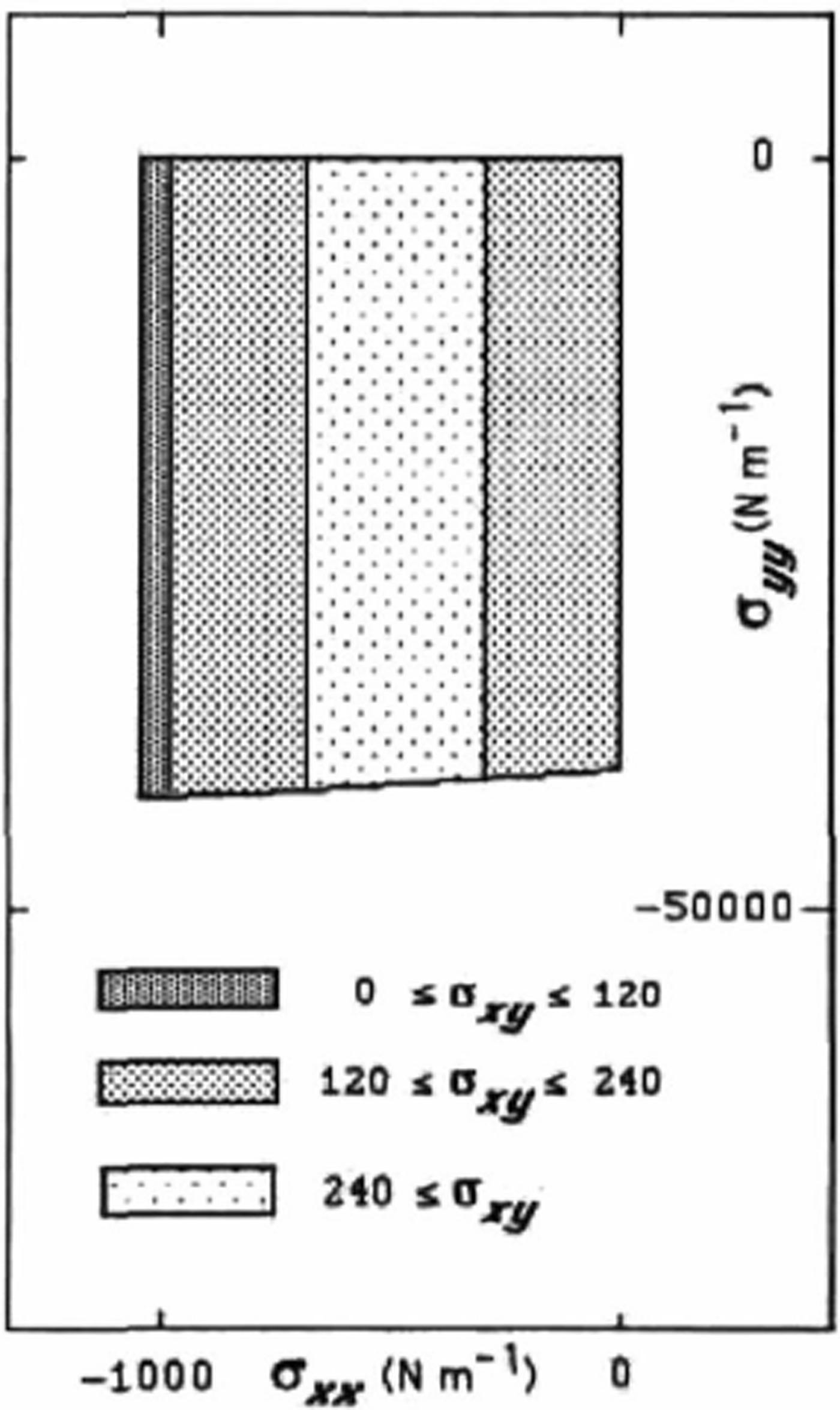
Fig. 2. Yield surface for a single lead embedded in thick ice with orientation as shown in Figure 1. All stresses have units of Nm−1 . The thick ice has strength P = 10 5 Nm −1 and comprises 99% of the area. The thin ice has a strength equal to 1% of the thick ice strength and comprises 1% of the area.
If we consider a strain rate with principal axes not aligned with the thin ice, then the stress and strain rate principal axes are no longer aligned and the behavior is more complex. Clearly, in general we need a yield surface (as shown in Figure 2), not just a yield curve to describe the system completely. What we see from the yield surface is that as σ xy increases, σ xx for compressive failure decreases. However, because of the extreme weakness of the lead in this case, there is little change in σ yy at failure.
In the work described here we are ultimately interested in isotropic response that takes into account the fracture and flow character of sea ice laced with cracks and leads. Consequently in the remainder of the paper we will consider only cases where the principal axes of stress and strain are aligned even though the system may be anisotropic. In this special case the yield characteristies may be described by a yield curve rather than a full yield surface.
Two or more leads
To consider the case of more than one lead is a straightforward extension of the single-lead equation. In particular, in this case, we simply need to rotate the strain to the lead coordinate system. The main difference, however, is that the strain along the lead is no longer the same as for the thick ice, but is now equal to the external compressive strain along this direction applied to the whole system. Also, the numerical solution requires a solution of linear equations at each iteration. Failure stresses may be obtained by specifying strain rates and solving for the stresses, or by specifying confinement-stress ratios as described in the next section.
The configuration for two leads is shown in Figure 3. Again, since we are interested in the most symmetric response, if we consider strains with principal axes aligned along the x and y directions as shown in Figure 3, the principal axes of stress will also be aligned in these directions. But, as in the single lead case, the response is decidedly anisotropic. The resulting yield curve for this system is shown in Figure 4, in the case of leads at an angle of ±18° relative to the y axis. We chose 18° because similar angles have often been observed for intersecting leads (e.g. Reference Marko and ThomsonMarko and Thompson, 1977). Note that for this case, the leads open up under lower confinement R = σ xx /σ yy ≤∼ 0.32 denoted by open circles) and close under higher confinement (denoted by ⊕). With regard to asymmetric strength, the asymptotic strengths for very low confinement may be understood in terms of a greater compressive stress on the lead leading to a greater shear stress needed for failure when σ yy ∼ 0 as compared to σ xx ∼ 0. However, as is the case in Figure 2, the precise limiting behavior for zero confinement is not well represented in Figure 4a. Also with this model, in contrast to the single-lead model, the thick-ice strength effectively plays no role in the failure stresses.

Fig. 3. Schematic view of two intersecting leads oriented symmetrically about the y axis.

Fig. 4. Yield curve and flow rule for two symmetric intersecting leads oriented at 18° relative to the y axis (see Fig. 3) for σxy = 0. Each lead comprises 0.4% of the area and has a strength equal to 1% of the thick ice strength P, which is equal to 105 Nm1. (a) Yield curve where circles with plusses indicate the thin ice leads are closing and open circles denote opening leads. (b) Angle between the strain-rate vector and the yield curve for σxx/σyy < 1. The flow angle is measured clockwise from the strain-rate vector to the tangent of the yield curve. Hence, angles < 90° correspond to greater convergence than the normal flow rule.
Some of the flow characteristics for this two-lead composite are shown in Figure 4b, where we have plotted the angle between the strain-rate vector and yield curve for |σ xx | < |σ yy |. As can be seen up to confinement ratios of about 0.09, the flow is more convergent than a normal flow rule would yield. The effective discontinuity at this confinement ratio arises from the truncated ellipse assumption for the thin ice (see Appendix), and occurs when the lead ice failure stress changes from uniaxial to biaxial. After this stress point, the flow is essentially more divergent than for normal flow with the maximum deviation from normality occurring where |σ yy | becomes maximum.
Failure and Flow of Cracked Sea Ice Relevant to Climate
The main goal here is to consider how fracture and flow of cracked sea ice affects the constitutive behavior of sea ice relevant to large-scale climate simulations. Consequently, utilizing the above theory, we wish to consider initially isotropic realizations with the main provision being that the failure and flow are dictated by the thin lead and/or crack structure. An implicit assumption here is that the strength of the aggregate is essentially controlled by the thin ice. Two cases of isotropic response can be considered. The most straight for ward case is to consider a uniform distribution of equally strong leads in all directions. In this case the response must clearly be isotropic, although the flow for the composite as a whole will be considerably different than a normal isotropic yield curve with normal flow rule. Also, as discussed below, depending on the stress state, the system will fail with the concemitant formation of two preferred leads or ridges.
A second case, which we feel is closer to laboratory measurements of the biaxial failure of fresh- and salt-water columnar ice, is the case where we allow "strain hardening" in the sense that only leads that have the potential to open rapidly are considered. The other leads are considered to have become stronger relative to the rapidly opening leads by freezing, or simply by opening less rapidly. In this strain hardening case the orientation of the selected leads will depend on the orientation of the applied stress state. However, since strain-hardened leads or ridges are generated by the stress state, the system is isotropic in the sense that it will behave the same under any direction of sustained loading, because the leads or cracks that become active will be picked out by the applied stress.
Since we are mainly interested in the response to a specified stress, to examine these two cases we will carry out numerical experiments in a manner similar to those conducted in the laboratory (Reference Schulson and NickolayevSchulson and Nickolayev, 1995). Specifically we consider a biaxial experiment with a fixed confinement stress ratio R = σ xx /σ yy and a fixed strain rate along the direction of the larger stress. The other strain rate is adjusted at each iteration so that the stress ratio remains fixed at each iteration. As in the laboratory, the numerical experiment then determines the magnitude of the stresses and strain-rate ratio.
Uniformly oriented leads
To approximate numerically the case of uniformly oriented leads of equal strength we consider a partition of 40 thin-ice leads at 4.5° intervals centered at values of θ ranging from θ = 85.5 to θ = 90°. Clearly, because of symmetry, we only need to consider a distribution spanning 180°. We then subject this system to different biaxial stress forcing as described above.
What we expect to happen with this configuration is that certain preferred orientations of leads (or ridges) will form depending on the stress confinement ratio. The concept is illustrated in Figure 5, where we use only two leads as illustrated in Figure 3, and numerically examine the stress component σ yy at failure as a function of lead-intersection angle for different fixed-stress confinement ratios R = σ xx /σ yy . Basically, for a given confinement ratio there is a lead-intersection angle that yields a minimum compressive stress for failure. This failure stress is lowest for low confinement ratios with the angle of intersecting leads at the minimum stress increasing as the confinement ratio increases.
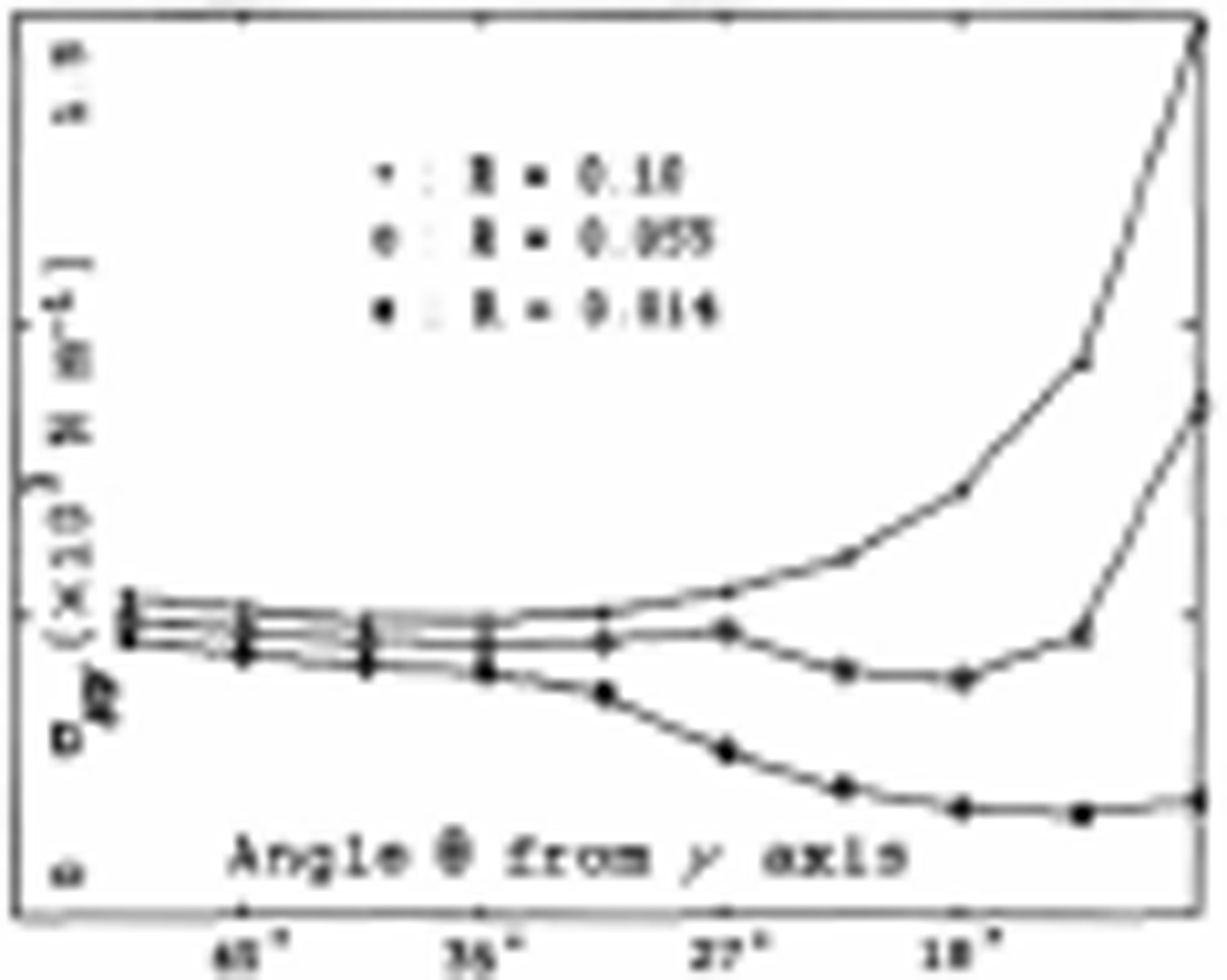
Fig. 5. Failure stress for two symmetric intersecting leads intersecting at angle 2θ for different stress-confinement ratios R = σxx/σyy. The leads each comprise 0.4% of the area and have a strength equal to 1% of the thick ice strength P which is equal to 105 Nm−1
An interesting feature of Figure 5 is that for intermediate confinement ratios of about 0.055 there are two minima — one at about 18° and one at 36°. At lower and higher confinement ratios, one of these minima disappear, without passing through an intermediate minima in between. As a consequence, with this uniform thin-ice-strength model, it is very difficult to get leads with angles 20.5 ≤ θ ≤ 36°.
Lead deformations resulting from the numerical experiments for a uniform distribution of equal strength leads are shown in Figure 6. Since with many leads the confinementratio experiments can, under certain circumstances, produce solutions at a local stress minima, in all the reported results, solutions corresponding to the lowest compressive stress were used. These multi-lead results confirm our expectations, namely that for this uniformly oriented set of leads, the deformation will occur preferentially across a specified set of intersecting leads. For low confinements, this deformation will take the form of rapidly opening pairs of leads with intersection angles decreasing to zero in the limit of no confinement. For higher confinement, this deformation takes the form of convergence, and hence ridge formation across a pair of leads with the intersection angle going to zero for high enough confinement. This low-confinement stress ratio for lead formation is consistent with stress observations by Reference Richter-MengeRichter-Menge (1997), which indicate low confinement ratios, especially during major stress events. Both these divergent patterns are accompanied by substantial concomitant shear across the same two particular leads. Note also that for both ridging (closing) and faulting (opening) deformation the rate of convergence (or divergence) is greater for smaller intersection angles.
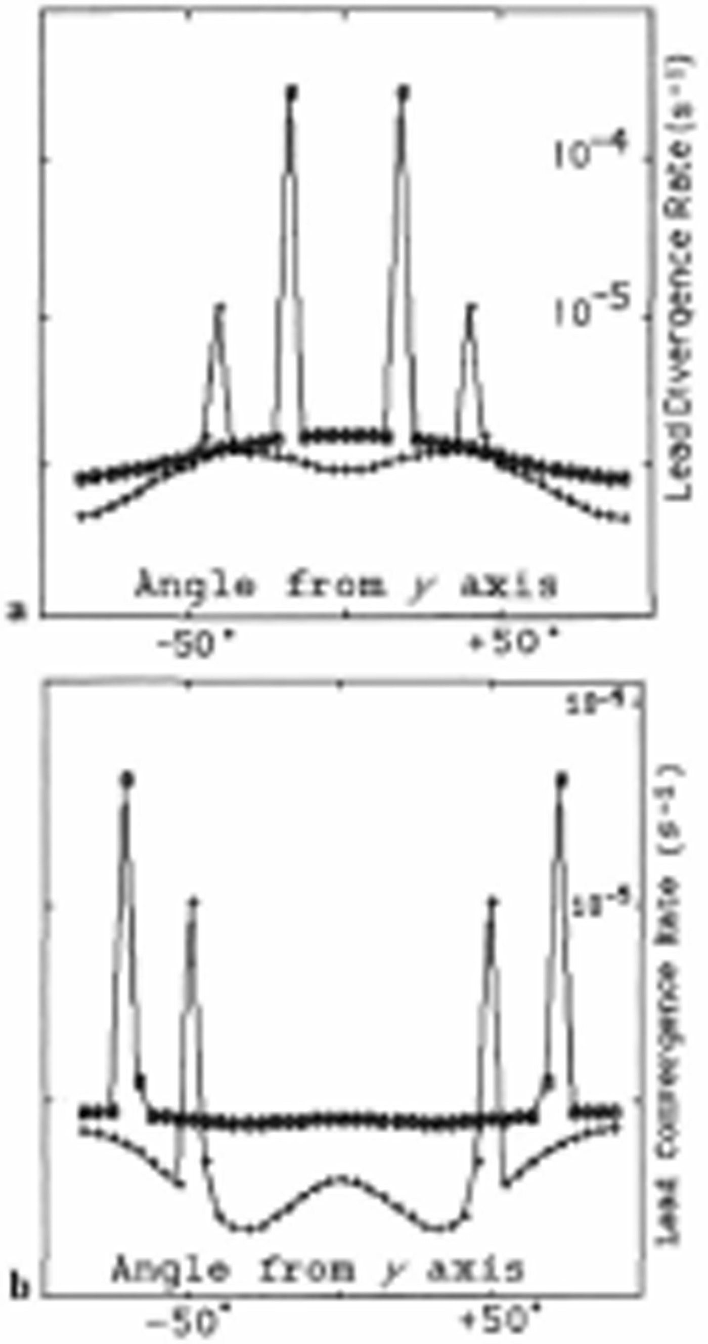
Fig. 6. (a) Rates of opening of leads vs angle for two different confinement ratios R = σxx/σyy = 0.025 (circles) and R = 0.25 (plusses). In order to do a logarithmic plot, a small constant (106 s1) has been added to the divergence rates so the ordinate is actually divergence rate + 10−6 s−1. (b) Rates of lead closing vs angle for confinement ratios of R = 0.44 (plusses) and R = 0.75 (circles). In all cases the overall strain rate imposed on the composite system along the y axis was έyy = −0.5 × 10⁻⁶ s−1. The composite consists of 40 leads with a uniform spatial distribution: i.e. θ ranging from −85.5° to 90°. Each lead comprises 0.4% of the area and has a strength equal to 1% of the thick ice strength P, which is equal to 105. N m−1.
The yield curve corresponding to this suite of numerical biaxial-confinement experiments is shown in Figure 7. These stresses are effectively independent of strain-rate magnitudes except for very small strain rates in keeping with the behavior of ice in the laboratory (Reference Schulson and NickolayevSchulson and Nickolayev, 1995). We emphasize that the normal flow rule does not apply to this composite system, although it is not drastically different. Note that the yield curve does intersect the principal stress axes at a non-zero value, which is substantially smaller than the intersection of the truncated ellipse for the thin ice (see Appendix). The general shape of the yield curve is close to the sine lens yield curve proposed by Reference BratchieBratchie (1984), based on kinematical considerations of discrete flow collisions. However, there is a slight asymmetry in the result here, with the yield curve being narrower near the origin.
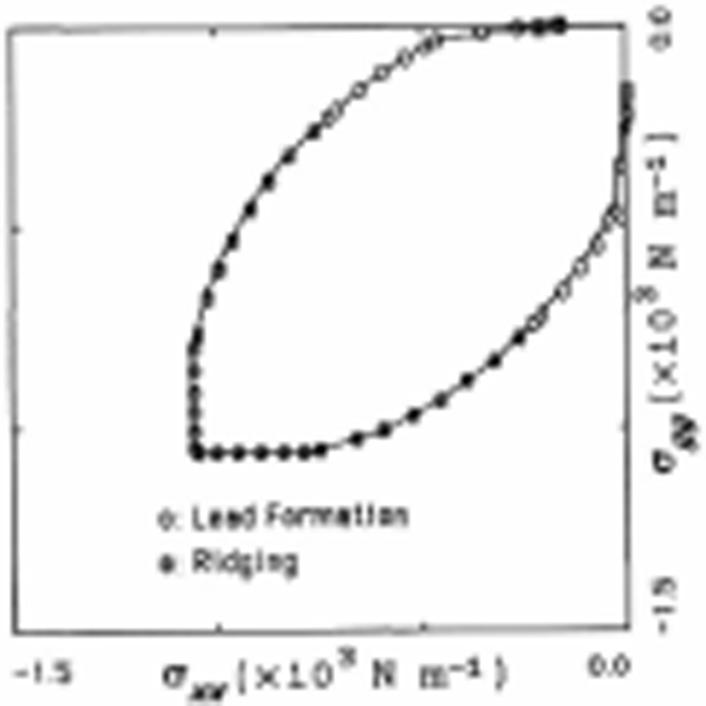
Fig. 7. Failure stresses for a composite consisting of 40 leads with a uniform spatial distribution (see Fig. 6 caption).
An approximate strain-hardening yield curve and flow rule
A key feature of the uniformly oriented multi-lead results was that certain leads open much more rapidly than others. If all the leads are of equal strength and penetrate through the same geographical region, then the slower opening leads would still fail. However for a larger region with leads of different orientations and in different locations with a distribution of strengths, we would expect higher confinement ratios to produce also opening of lower intersection angle leads that can open faster, ultimately forming cracks through the whole system. For example, let us imagine a region of ice with a set of weak 18° leads and slightly stronger 36° leads, so that both leads may open under the same confinement stress. As the strain proceeds the 18° leads will open rapidly and likely propagate. Consequently the 36° leads will effectively become "stronger" relative to the 18° leads as the strain proceeds. Hence we can consider, under strain, the 36° leads to be strain hardened relative to the 18° leads. The effective yield curve resulting from sustained loading, over say one day, would therefore be similar to that obtained if the 36° leads were removed to begin with. This concept, plus the results of Figure 5 indicating a "barrier" at about 20°, suggest a model where we consider only leads with an orientation ≦ 18° relative to the main applied stress. As we shall see below, this assumption also generates a yield curve that is substantially similar to that obtained from laboratory experiments.
Numerical experiments with this ≦ 18° model result in a yield curve very similar to that in Figure 4, and with the deformation almost always occurring across the 18° leads except for very small confinement ratios. However, since we are postulating that far-field applied stress induces the orientation of leads, the response will be symmetric rather than anisotropic as in Figure 4. Also, at some point for sufficient confinement, when out-of-plane failure likely occurs, it is expexted that there will be no preferred direction for the leads. Where this confinement occurs is not clear, so we arbitrarily pick the confinement where the convergence and maximum shear in the 18° leads are approximately equal. (Picking a lower confinement would not, however, change the essential features of the following results.) This confinement occurs around R = σ xx / σ yy ∼ 0.5. For higher confinement, the convergence in the leads exceeds the shear deformation and we would expect it to be difficult for the lead to maintain itself or to propagate. In the laboratory, the failure mechanisms for high confinement are different from the crack-shear mode (i.e. out-of-plane spalling instead of in-plane macroscopic shear faulting).
To allow biaxially convergent strain rates to be modeled we need to close the yield curve past this critical confinement point. To do this we may fit an elliptical yield curve (not necessarily with a normal flow rule) to the fracture-based yield curve in a way that allows both the stress and flow to vary smoothly. This can be done by the appropriate choice of eccentricity, strength and pressure. Once this is done, the eccentricity and pressure can be adjusted to obtain the stress rates on the fracture-based yield curve corresponding to a given strain rate. Hence a set of bulk and shear viscosities and pressure as a function of strain-rate invariants can be constructed that map out the isotropic fracture-based yield curve.
Results of carrying out this fitting procedure at one point are shown in Figures 8 and 9. The flow characteristies are shown in Figure 8 by plotting the ratio of strain-rate invariants vs stress-invariant ratios for the strain-hardening yield curve. These particular invariants were chosen in order to obtain a single valued function over the yield curve. For comparison, we have also plotted the flow characteristies of the truncated ellipse (see Appendix). The lead-based model has a greater opening rate than the truncated ellipse model when leads are opening, and a greater closing rate when convergence is occurring. To extend the flow and failure curves past the point where there is biaxial convergence, we have fitted an elliptical yield curve to this stress point in such a manner that the stress and strain rates vary smoothly.
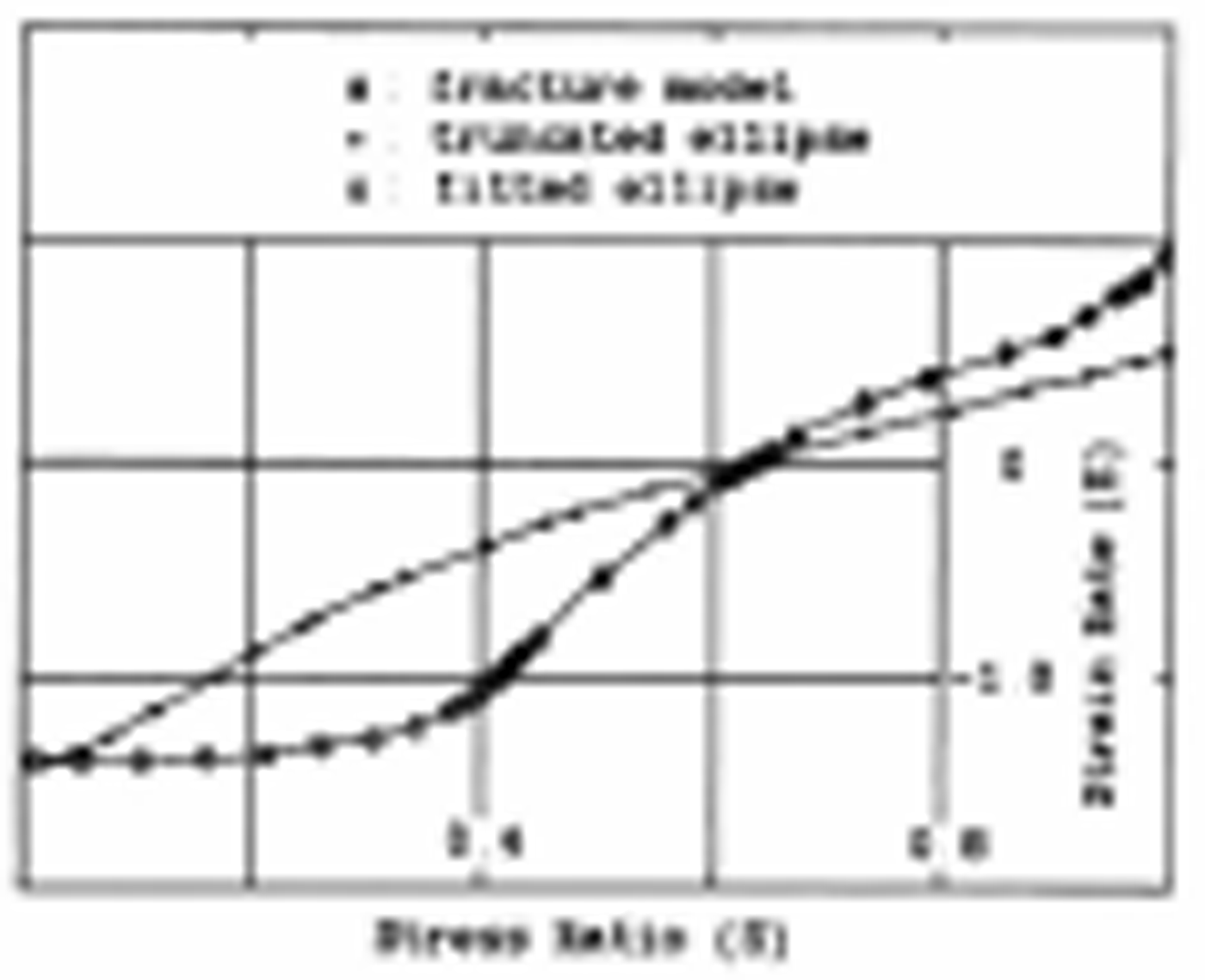
Fig. 8. Strain-rate invariants ![]() vs stress invariants
vs stress invariants
![]() for isotropic truncated elliptical yield curve (pluses) and
for "strain-hardening" lead model (zeros) consisting of
leads < 18 relative to the principal applied
stress direction. In the strain-hardening model each lead
comprises 0.4% of the area and has a strength equal to 1% of the
thick ice strength P, which is equal to 10
N m
l
. In all cases σ
xy
= έ
xy
= θ and έ
yy
< θ. The circles denote an elliptical yield curve
that has been smoothly filled to the "strain-hardening" model at
the point where έ
xx
changes from positive to negative values, i.e. E =
−1.
for isotropic truncated elliptical yield curve (pluses) and
for "strain-hardening" lead model (zeros) consisting of
leads < 18 relative to the principal applied
stress direction. In the strain-hardening model each lead
comprises 0.4% of the area and has a strength equal to 1% of the
thick ice strength P, which is equal to 10
N m
l
. In all cases σ
xy
= έ
xy
= θ and έ
yy
< θ. The circles denote an elliptical yield curve
that has been smoothly filled to the "strain-hardening" model at
the point where έ
xx
changes from positive to negative values, i.e. E =
−1.
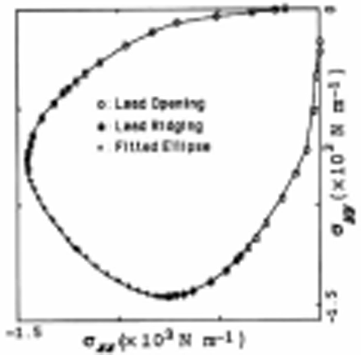
Fig. 9. Isotropic yield curve for the "strain-hardening" model consisting of weak leads at angles < 18° relative to the principal applied stress direction (see Fig. 8 caption). An elliptical yield curve has been fitted to the fracture-based yield curve beginning approximately at the maximum compressive stress in the y direction (for R = σ xx /σ yy < l) and at a symmetric point for R > l.
The composite-stress failure curve resulting from this fitting procedure is shown in Figure 9, where the points past the minimum value of |σ yy | (for R = σ xx /σ yy < 1) denote the fitted elliptical curve. Other values are taken entirely from the ≤ 18 lead model. This type of yield curve bears a substantial resemblance to that obtained in the laboratory for conditions where cracking dominates the failure process. For large-scale simulations, it has a number of useful characteristies, not least of which being that it will predict interseeting lead orientation and intersecting slip lines. Since the failure characteristics are now based on an anisotropic lead-based theory, the opening rates should be more realistie. Moreover, the system is isotropic in character, so that it can be modeled within existing model formulations.
Concluding Remarks
The main purpose of this paper has been to develop a conceptual base for the inclusion of fracture-based flow in seaice rheologies relevant to numerical investigations of elimate. The essential idea is to make use of oriented weak leads or flaws embedded in thicker ice. By assuming a viscous-plastie constitutive law for both the thin and thick ice and insisting on continuity of stresses, anisotropie yield and flow characteristies of this composite system may be numerically obtained.
To examine some of the characteristies of collections of oriented weak leads embedded in thick ice, two isotropie realizations of this composite model were examined: an isotropic-lead model with uniformly oriented leads in all directions, and an approximate strain-hardening model where only oriented leads that have the potential to open rapidly were allowed. The uniform–orientation model resulted in a yield curve that approximates a sine lens. The strain-hard-ening yield curve is more of teardrop shape, and bears a substantial similarity to laboratory-based biaxial yield curves. In both these isotropic cases, simulations naturally predict preferential opening and/or closing of different oriented pairs of leads depending on the nature of the stress state. Specifically, opening occurred up to stress-confinement ratios R = σ xx /σ yy of about 0.3. whereas higher confinement ratios led to ridging and shearing. Also, the precise amount of opening and closing of individual leads which may differ from the overall deformation is accounted for.
While these isotropic cases incorporate fracture-based failure mechanisms, they can, in principle, be relatively straight forwardly used in existing large-scale sea-ice dynamics models developed for climate studies by utilizing the appropriate dependence of the non-linear viscosities and pressure on the strain-rate invariants. The coupling of the dynamical equations with ice-thickness evolution equations could then be carried out in the same manner as currently used in most large-scale models (see e.g. Reference HiblerHibler, 1979; Reference Flato and HiblerFlato and Hibler, 1992) where one strength is assigned to the whole composite. How this dynamical fitting procedure might be carried out was outlined in the case of the strainhardening model.
Simulations using variations of this model to solve the full sea-ice-dynamies equations and predict lead patterns for the Aretie Basin are currently underway. More complete numerical comparisons to laboratory observations are also needed to establish a more precise physical basis for the idealized strain-hardening model. We hope the work described here will provide the motivation and framework for other similar investigations.
Acknowledgements
This work was supported by the Office of Naval Research under Contracts N00014-96-1 and N00014-92-J-1279.
Appendix
For the constitutive law applying to the thin and thick ice we make use of an elliptical yield curve modified to have no tensile stress. For an elliptical yield curve following Hibler (1979) the stress is given by:
where repeated subscripts are summed over and η and ζ are functions of the strain rate according to:
where

P * is the ice strength (equal to the pressure P for high strain rates) and e is a constant taken to be 2 in all simulations done here. To approximate rigid stress states inside the yield curve, ζ and η are capped at some large maximum value (see Hibler, 1979) for small strain rates.
The basic principle in the truncated ellipse is to reduce the shear viscosity in such a way that the maximum shear stress is reduced to prevent any tensile stress from occurring. Referring to Figure 10, the condition we wish to enforce is:
in such a way that
With the viscous-plastic rheology σ 1 is given by:
where έ 1 and έ 2 are the principal components of the strainrate tensor.
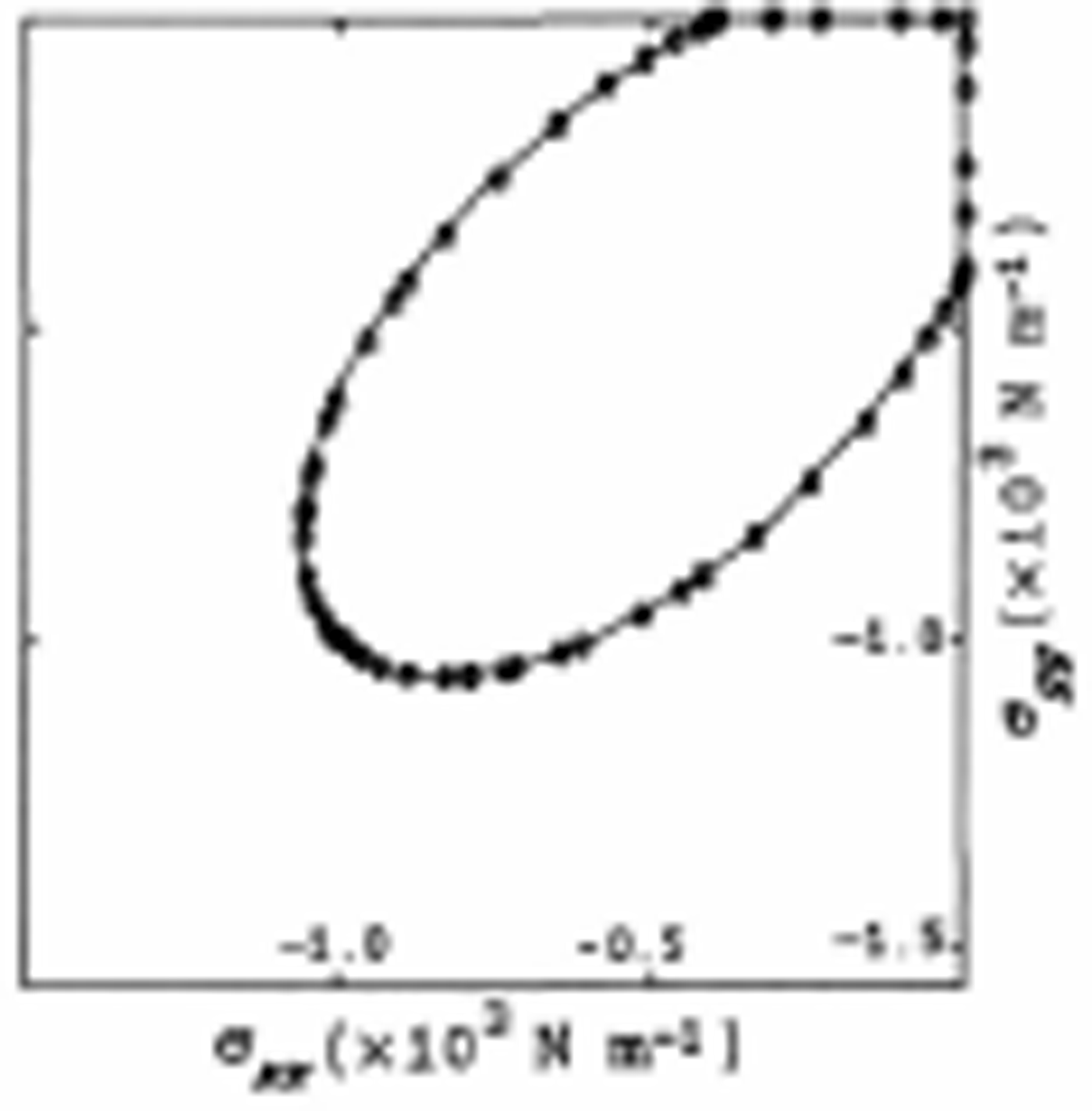
Fig. 10. Truncated elliptical yield curve for isotropic thin ice having a strength of P = 103 N m 1
If we choose η such that
then the condition in inequality (Equation (A1)) will always be met. To ensure that there is no stress at zero strain rates we insist the P = 2Δζ where
When plastic flow is occurring, P will be a constant (P *), but for ζ = ζ max the stress state will lie on a smaller geometrically similar truncated ellipse to Figure 10 going through the origin.
This overall procedure will generate a rheology with no tensile stress and a substantially reduced ice-shear stress under divergent conditions than occurs with the conventional elliptical yield curve.


