Paleobiogeographic insights gained from ecological niche models: progress and continued challenges

Abstract

The spatial distribution of individuals within ecological assemblages and their associated traits and behaviors are key determinants of ecosystem structure and function. Consequently, determining the spatial distribution of species, and how distributions influence patterns of species richness across ecosystems today and in the past, helps us understand what factors act as fundamental controls on biodiversity. Here, we explore how ecological niche modeling has contributed to understanding the spatiotemporal distribution of past biodiversity and past ecological and evolutionary processes. We first perform a semiquantitative literature review to capture studies that applied ecological niche models (ENMs) to the past, identifying 668 studies. We coded each study according to focal taxonomic group, whether and how the study used fossil evidence, whether it relied on evidence or methods in addition to ENMs, spatial scale of the study, and temporal intervals included in the ENMs. We used trends in publication patterns across categories to anchor discussion of recent technical advances in niche modeling, focusing on paleobiogeographic ENM applications. We then explored contributions of ENMs to paleobiogeography, with a particular focus on examining patterns and associated drivers of range dynamics; phylogeography and within-lineage dynamics; macroevolutionary patterns and processes, including niche change, speciation, and extinction; drivers of community assembly; and conservation paleobiogeography. Overall, ENMs are powerful tools for elucidating paleobiogeographic patterns. ENMs are most commonly used to understand Quaternary dynamics, but an increasing number of studies use ENMs to gain important insight into both ecological and evolutionary processes in pre-Quaternary times. Deeper integration with traits and phylogenies may further extend those insights.

Non-technical Summary

The spatial distribution of species across the landscape and their associated traits and behaviors play a pivotal role in determining ecosystem structure and function and contribute to our understanding of the processes that shape biodiversity. Ecological niche models (ENMs) are tools that can be used to estimate the ecological niche of a species based on its known occurrences. In this review, we explore the ways that ENMs have been used to study the evolution and ecology of past biodiversity. While ENMs are commonly used to understand the dynamics of species and assemblages during more recent periods of Earth history (i.e., the last several million years), an increasing number of studies have extended ENMs deeper into the geologic past. Overall, ENMs are powerful tools for illuminating paleobiogeographic patterns; further integration of ENMs with traits, phylogenies, and other methods may extend insights.

Introduction

The spatial distribution of individuals within ecological assemblages and their associated traits and behaviors are key determinants of the structure and function of ecosystems and, ultimately, the services they provide, which support life on Earth (e.g., Cardinale et al. 2012; Tilman et al. 2014; van der Plas 2019). Thus, biodiversity is, and has always been, a key regulator of planetary homeostasis (Mace et al. 2014; Steffen et al. 2018; Talukder et al. 2022). Understanding where and why different species exist—now, in the past, and in the future—reveals how that regulation operates and how humans have altered it (Lyons et al. 2016; Barnosky et al. 2017). Determining the spatial distribution of different species, and how distributions influence the spatial patterns of species richness across different ecosystems today and in the past, helps us understand what factors act as fundamental controls on biodiversity.

Where species occur reflects aspects of their environment (e.g., Grinnell 1917; Hutchinson 1957; Colwell and Rangel 2009; Soberón and Nakamura 2009). This correspondence between species and environment has been used to understand the factors supporting species’ persistence (e.g., Holt 2009; Scheele et al. 2017), to examine the interactions between species (e.g., Wiens 2011; Blois et al. 2013), and to infer past climates and other environmental conditions (Fagoaga et al. 2019; Chevalier et al. 2020; Wei et al. 2020). Today, this relationship is increasingly being used to predict potential future ranges of species, given global anthropogenic climate change (Dietl and Flessa 2011; Kuemmerle et al. 2012; Lima-Ribeiro et al. 2017; Ivory et al. 2019).

Since the inception of Paleobiology 50 years ago, and particularly over the last few decades, scientists have used ecological niche models (ENMs) to define species–environment relationships. We expand on definitions of the niche, our use of the term “ENMs”, and related terms in Box 1. In short, ENMs are statistical models in which species’ occurrences are related to different aspects of the climate or resources (collectively, “the environment”) and are used to infer species’ niches (Guisan and Thuiller 2005; Elith and Leathwick 2009; Holt 2009; Fig. 1). Species’ occurrences are sourced from field surveys, primary literature, museum records, or often through databases that aggregate these occurrences, such as the Global Biodiversity Information Facility (GBIF; https://www.gbif.org), the Neotoma Paleoecology Database (https://www.neotomadb.org; Williams et al. 2018), and the Paleobiology Database (PBDB; https://paleobiodb.org). This correlative approach does not guarantee that all factors supporting a species’ persistence (i.e., its fundamental niche) will be captured. However, by statistically characterizing the relationships between species’ occurrences and the environment, it is possible to identify a subset of environmental factors that are strongly associated with species’ presence (Fig. 1A) and thus approximate the species’ niche (i.e., its “realized” niche; Fig. 1B). This statistical relationship allows us to investigate why species are found in some places or environments and not others (Fig. 1C), providing better insights into the fundamental controls on species’ distributions and enabling forecasting of future distributions.

Box 1. Definitions of terms

The concept of a niche (sensu Chase and Leibold 2003) encompasses both the set of resources that support population stability and/or growth (the “Grinnellian” niche; Soberón 2007) as well as the per capita impacts that a species has on those resources (the “Eltonian” niche; Soberón 2007). Although acknowledging both, our primary focus in this paper is on the Grinnellian niche, which we will refer to simply as “the niche” henceforth.

Understanding species’ niches has been a pursuit spanning centuries. The definition of the Grinnellian niche was formalized by Hutchinson (1957) as an n-dimensional hypervolume, typically characterized by multiple environmental factors that support species’ persistence. The n-dimensional hypervolume is now commonly used to examine spatiotemporal patterns in species’ niches and distributions, although defining species’ requirements and tolerances is simple in concept but often difficult in practice. Today, ecological niche models (ENMs) play a crucial role in estimating species’ niches by defining species–environment relationships. ENMs are statistical models, wherein current species’ occurrences (e.g., modern-day presence, presence/absence, abundance) are related to diverse environmental factors, such as contemporary climate, resources, and other relevant variables, collectively termed “the environment” (Fig. 1A). ENMs come in a variety of forms, encompassing both parametric and nonparametric approaches.

Under a parametric framework, ENMs commonly employ regression-type analysis. Here, species occurrences serve as the dependent variable, while environmental factors such as climate and vegetation act as independent variables within the model equation. The resultant statistical relationships, depicted as response curves, delineate the species’ niche within a multidimensional environmental space defined by environmental variables included in the ENM (Fig. 1B). These curves convey the probability of events, such as a species’ occurrence, at distinct points within the environmental space. Within a nonparametric framework, methods like kernel density estimation (KDE) can be utilized to build ENMs. KDE generates a continuous probability density function (PDF) based on a finite set of observations (i.e., species’ occurrences) along one or more independent environmental axes. Integrating this PDF over specified intervals yields the probability of events occurring within those environmental ranges. Both parametric and nonparametric methods can be employed across one or more environmental dimensions.

While ENMs are calibrated on present-day data, we define paleoecological niche models (paleoENMs) as ENMs trained on paleo-occurrences and corresponding paleoenvironmental layers. In essence, paleoENMs leverage the fossil record for species’ occurrence data and utilize past environmental data that align spatially and temporally with the fossil record to obtain past species–environment relationships. Note that, while the paleoenvironmental data incorporated into paleoENMs can derive from various sources (see “Environmental Reconstruction” section), we do not differentiate between these data types but rather consider them collectively as paleoenvironmental information. In both ENMs and paleoENMs, model validation typically involves evaluating the model’s performance by comparing its predictions against an independent dataset.

Species–environment relationships estimated with ENMs or paleoENMs can then be used to project environmental suitability or species probability of occurrence within a multidimensional environmental space or across geographic space (Fig. 1C). The term “projection” encompasses forecasts, hindcasts, and projection to contemporaneous times. Forecasts are projections of niche models to time periods subsequent to the period in which the ENM or paleoENM was developed, while hindcasts are projections to time periods preceding the interval for which the ENM or paleoENM was developed. We note that if projections are made in geographic space, then the ENM could become a species distribution model (SDM). While the terms SDM and ENM are often used interchangeably in the literature, we consider SDMs to be a subset of ENMs, with the explicit intent of modeling geographic distributions, which often requires additional information on a species’ dispersal potential and biotic factors, while defining ecological niches via ENMs does not require these as inputs.

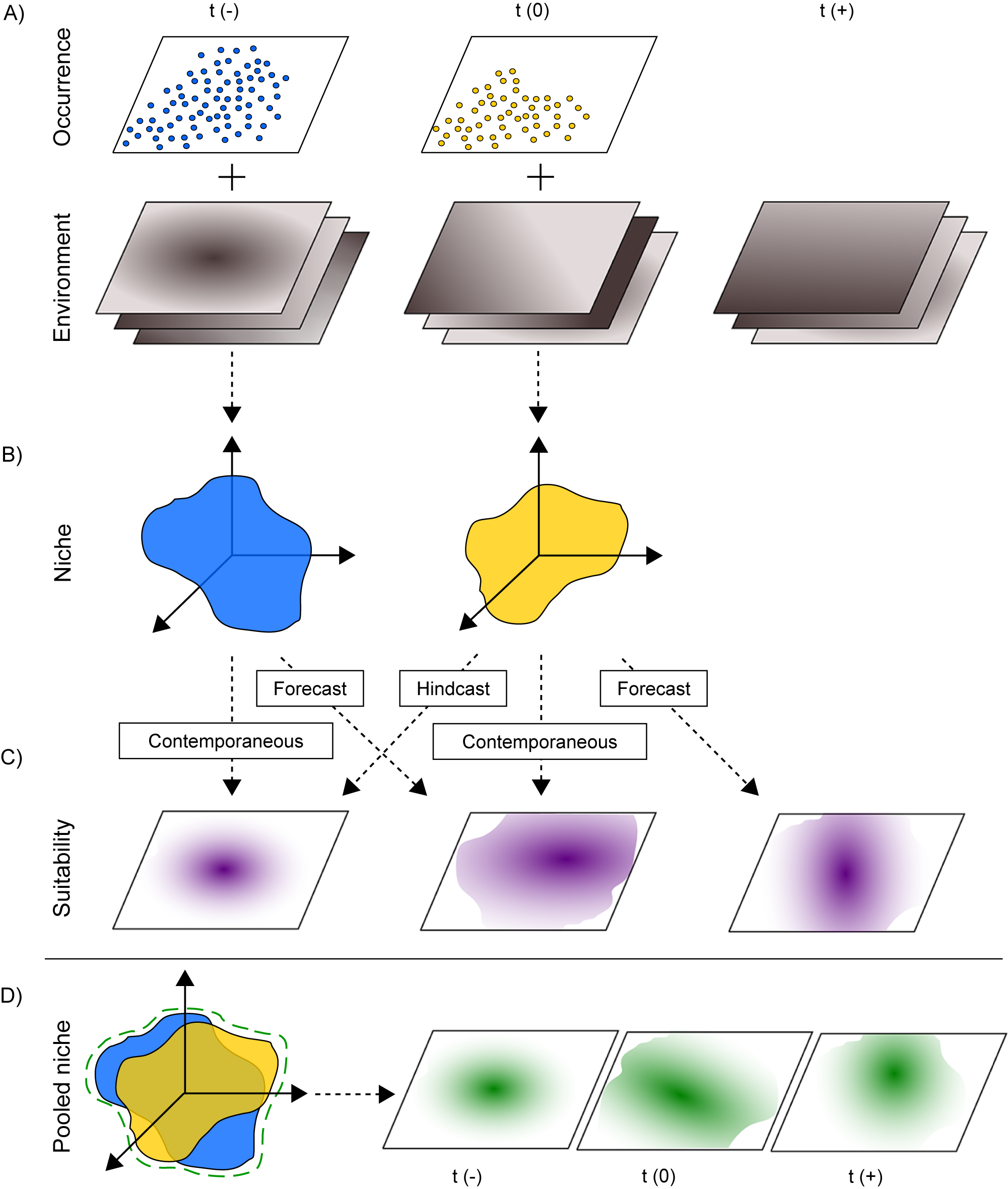
Figure 1. Ecological (ENMs) and paleoecological (paleoENMs) niche models integrate (A) species occurrence data with environmental layers to obtain (B) characterizations of species niches within an n-dimensional environmental space across time. Those niches are then (C) projected either contemporaneously or through hindcast (before the time interval for which ENM/paleoENM was developed) and forecast (subsequent to the time interval for which ENM/paleoENM was developed) projections to assess habitat suitability either in the original niche space or in geographic space. For a more accurate representation of species’ fundamental niches, (D) aggregating occurrences across multiple time periods generates pooled niches that can be used for projections into distinct time intervals.

A variety of past reviews have illustrated that inclusion of data collected across different times and environments, particularly from past environments without any contemporary analogue (i.e., paleoecological niche models [paleoENMs]; Box 1), allows for more complete characterization of the niche and thus better understanding of paleobiogeography (Nógues-Bravo 2009; Maguire et al. 2015; Myers et al. 2015; Lima-Ribeiro et al. 2017). PaleoENMs are not a panacea and indeed are subject to a variety of challenges akin to those encountered in ecological niche modeling more broadly (e.g., Guisan and Thuiller 2005; Elith and Leathwick 2009; Saupe et al. 2012). For example, limited fossil occurrences may exacerbate the issue of low sample size in paleoENMs, while taphonomic biases may make it difficult to interpret data on species’ absences. Furthermore, paleoecological niche modeling is typically not possible for taxa that do not readily fossilize. In addition, environmental layers are typically lower resolution and not as easily obtainable for time periods of the past as they are for the present day (Nógues-Bravo 2009; Svenning et al. 2011; Varela et al. 2011; Maguire et al. 2015; Myers et al. 2015), which has prompted the development of alternative methods based on sedimentary and stratigraphic characteristics (Stigall 2023; Holland et al. 2024). Despite these challenges, niche modeling is an extremely useful tool for paleobiogeography, and better integration of fossil data into ENMs has the potential to provide a deeper understanding of species’ niches, species distributions, and past biogeographic patterns.

Here, we explore how ecological niche modeling has been used to understand the spatiotemporal distribution of biodiversity in the past. The conceptual framework underlying ENMs and paleoENMs has been examined previously (Guisan and Thuiller 2005; Soberón and Nakamura 2009; Myers et al. 2015), and a series of excellent reviews has highlighted the strengths and challenges of modeling past species’ distributions and niches (Nógues-Bravo 2009; Svenning et al. 2011; Varela et al. 2011; McGuire and Davis 2014; Maguire et al. 2015; Myers et al. 2015; Moreno-Amat et al. 2017) and the paucity of studies incorporating fossil data into ENMs (Nógues-Bravo 2009; Svenning et al. 2011; Varela et al. 2011). We first assess the state of paleo-niche modeling through a semiquantitative literature review (SQLR), asking whether progress has been made in the past 10+ years in addressing previously outlined challenges of paleoENMs. We next discuss advances in technical development of paleoENMs, and then move toward a detailed overview of how paleoENMs have advanced our understanding of ecological and evolutionary patterns and processes. Finally, we explore emerging frontiers in niche-modeling approaches to paleobiogeography.

Semiquantitative Literature Review

To anchor our review, we conducted a search on 15 September 2023 for peer-reviewed articles, written in English, that applied ENMs to past time intervals using both the Scopus and Web of Science databases with near-identical search conditions (see Supplementary Appendix 1 for full search terms). Our search and screening followed the PRISMA protocol for scoping reviews (Tricco et al. 2018). Article metadata were downloaded from each database (Scopus n = 16,155, Web of Science n = 15,600), and the two datasets were merged and duplicates removed (n = 22,656). We screened article titles and abstracts to determine if they (1) projected an ENM to a point in time before 1800 C.E. and/or (2) included fossil occurrences in their ENM. We identified 668 studies that met our criteria and randomly assigned these to the five authors to gather data on the ENM approaches therein. Data extracted from each article included taxonomic information (taxonomic description and resolution, and the number of taxonomic units analyzed), time periods for which data were modeled and projected, use of the fossil record for either model calibration or validation, additional data (molecular, isotopic, morphological, etc.) used, and the geographic extent of the analysis. All data manipulation and analyses were performed in R (v. 4.3.0; R Core Team 2014) using an RStudio interface (v. 2023.06.1 Build 524 “Mountain Hydrangea”; RStudio Team 2020). Data manipulations were carried out with dplyr (v. 1.1.2; Wickham et al. 2023a), tidyr (v. 1.3.0; Wickham et al. 2023b), and stringr (v. 1.5.0; Wickham 2023). Title and abstract screening was done through revtools (v. 0.4.1; Westgate 2019).

Fossil evidence can be used in one of two ways in niche-modeling approaches: as occurrences during model training to infer the ecological niche and (potentially) geographic distributions (defined here as paleoENMs; Box 1) and/or to validate hindcast or forecast projections (Box 1, Fig. 1). We found that while the number of studies that apply ENMs and paleoENMs to understand past niches and distributions has increased and niche modeling is now a common tool in many different facets of paleobiogeography, ENMs that rely on fossil evidence in some way are still proportionately rare and appear to have reached a “steady state” (Fig. 2). Slightly more studies employing ENMs for paleobiogeography focus on animals than on plants, and a higher proportion of animal-based ENMs or paleoENMs incorporate fossil evidence into the niche models versus hindcasting ENMs to the past from contemporary occurrences (Fig. 3A). Most ENMs developed for paleobiogeographic studies are combined with some other approach, but studies that use just ENMs or paleoENMs are more likely to incorporate fossil evidence into their methods (Fig. 3B). The vast majority of paleobiogeographic studies that use niche modeling are focused on the regional scale and concerned with the Quaternary (Figs. 4, 5), although there has been a steady trend toward using niche-modeling approaches in paleobiogeography at older times (Fig. 5B). We examine these patterns in more depth in the subsequent sections.

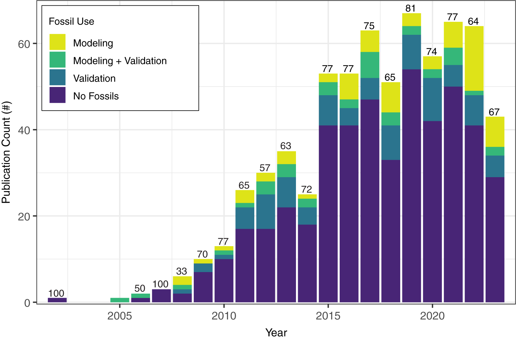
Figure 2. Stacked bar chart of the number (#) of publications that applied ecological niche models to past time intervals, ordered by publication year and categorized and colored by the authors’ use of fossils. To facilitate comparison of change in the proportion of publications that did not rely on fossil data in any way, the values listed above the bars show the rounded percentage of publications in the “No Fossils” category for each year.

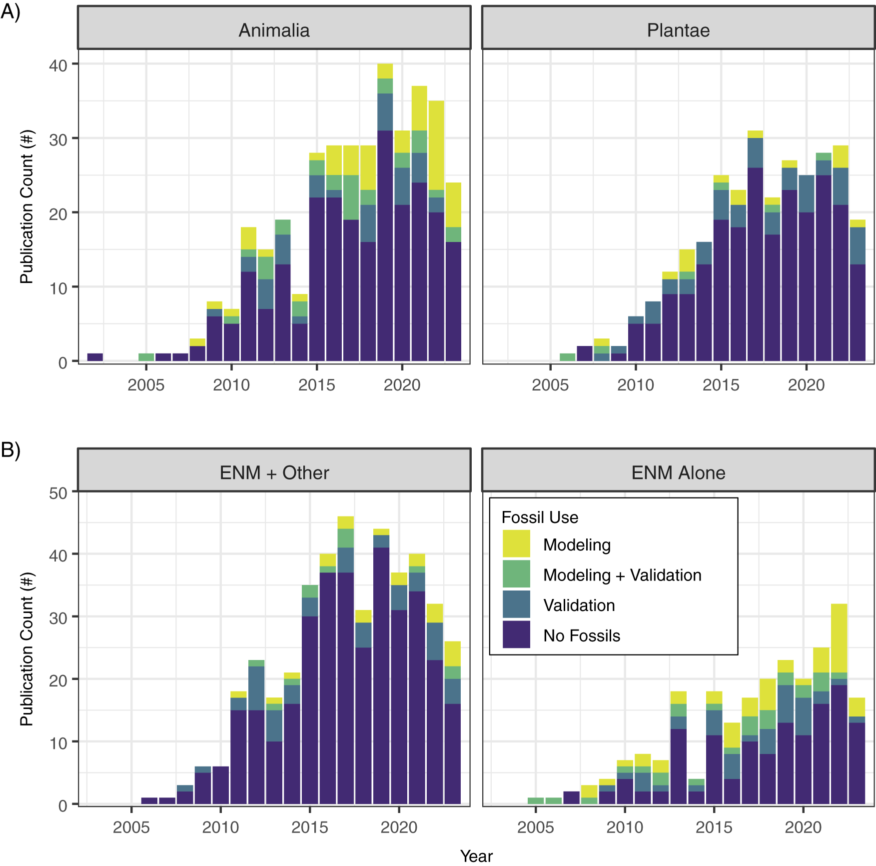
Figure 3. Stacked bar chart of the number (#) of publications that applied ecological niche models to past time intervals, ordered by publication year and showing (A) the number of publications focused on the Animalia and Plantae kingdoms, and (B) the number of publications that combined ecological niche models (ENMs) with other lines of evidence or where ENMs were the sole approach used in the study.

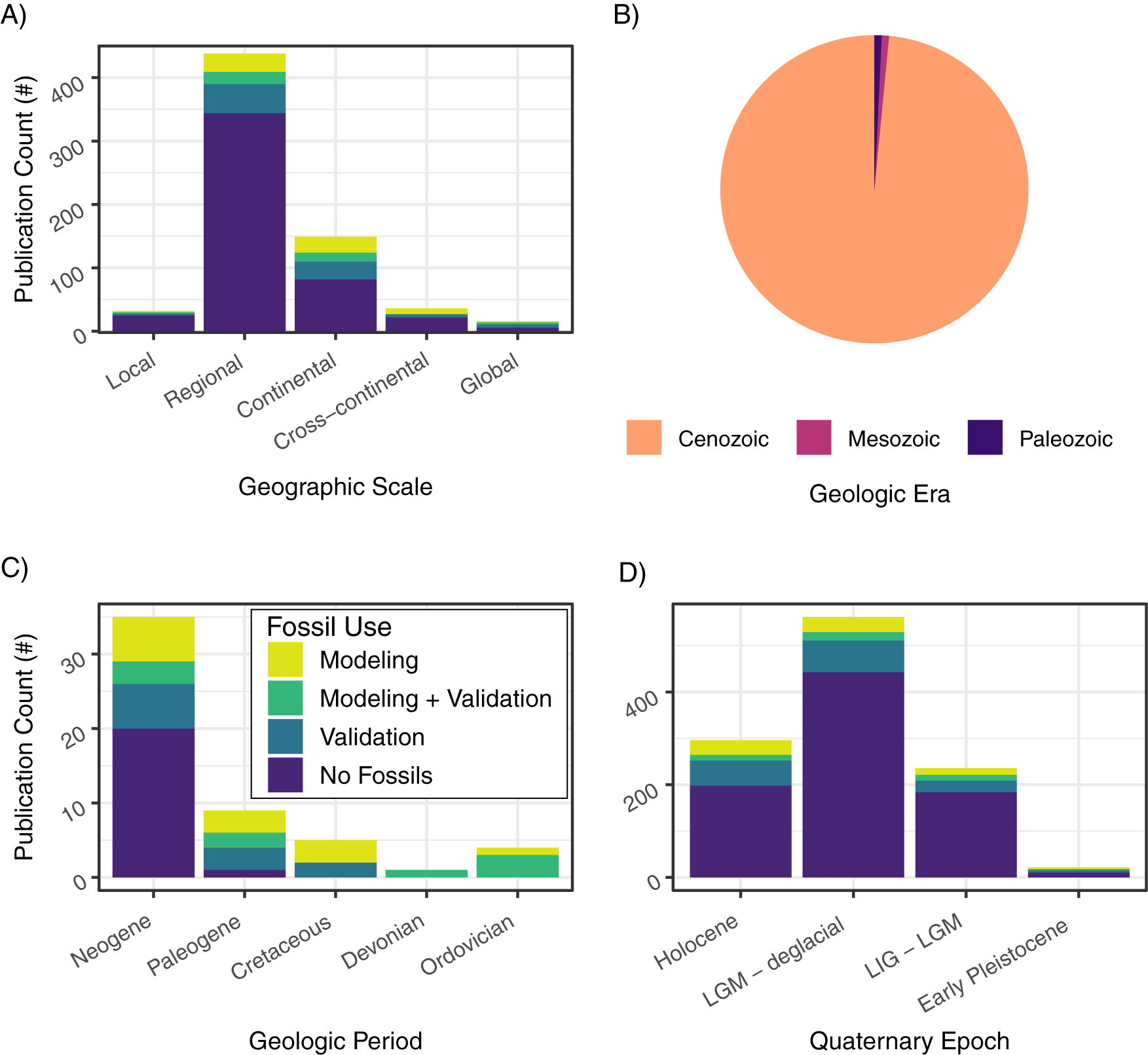
Figure 4. Stacked bar chart of the number (#) of publications that applied ecological niche models (ENMs) to past time intervals, ordered by publication year and categorized and colored by their use of fossils, showing (A) the number of publications focused on different geographic scales; (B), the number of publications focused on different geologic eras; (C), the number of publications focused on different geologic periods (excluding the Quaternary); and (D), the number of publications focused on different time intervals within the Quaternary: Holocene, 11.7–0 ka; LGM – deglacial, 22–11.7 ka; LIG – LGM, 140 – 22ka; early Pleistocene, 2.6 Ma–140 ka. LGM: last glacial maximum; LIG: last interglacial.

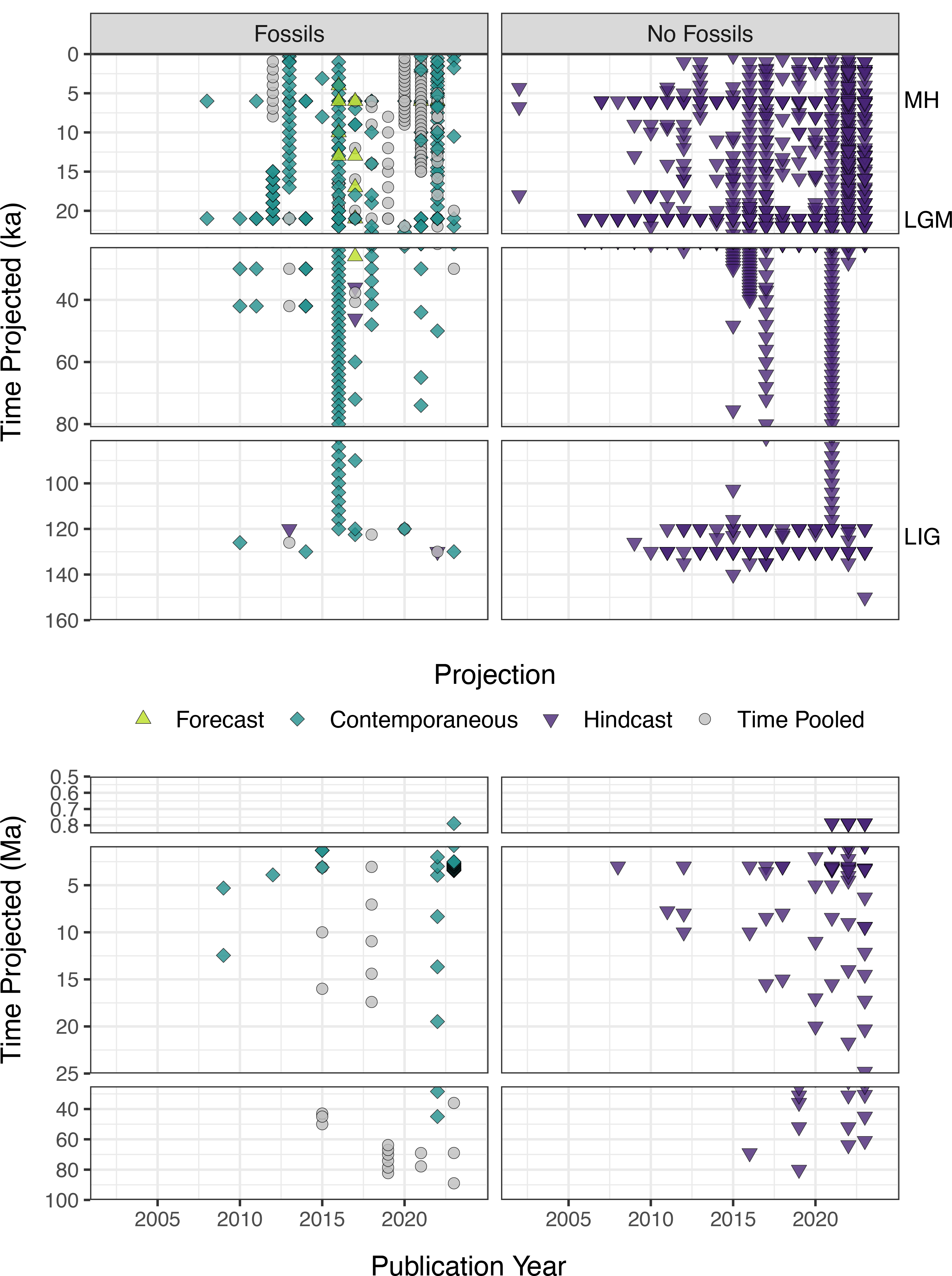
Figure 5. Trends across publication year in the times to which ENMs or paleoENMs are projected, focused on the subset of studies that project to (A) the last 160 kyr and (B) older periods in Earth history (0.5–100 Ma). Note that due to sparse data, we do not show the subset of studies that project to times older than 100 Ma. Studies that used fossils for either model development or model validation are shown on the left, and studies that did not rely on fossil evidence are shown on the right. Each color plus symbol combination shows the type of model (Fig. 1). Three time periods with widely available environmental layers are indicated on the right. For example, studies that incorporate fossil evidence can be either hindcast, forecast, or projected to contemporaneous times, whereas all studies that did not use fossils are necessarily hindcast to the past from the present. MH, mid-Holocene; LGM, last glacial maximum; LIG, last interglacial.

Advances in PaleoENM Methods

Several key reviews have highlighted the potential of paleoENMs in paleobiogeography (Dietl and Flessa 2011; Svenning et al. 2011; Varela et al. 2011; Franklin et al. 2015; Maguire et al. 2015; Myers et al. 2015; Moreno-Amat et al. 2017), but these reviews also illustrated some key concerns of ENMs and paleoENMs that may limit their utility. Here, we examine several key areas related to the technical development of paleoENMs that have seen major advances in recent years and that are particularly relevant to paleobiogeography: taphonomic biases, small sample sizes and taxonomy, environmental reconstructions, and model transferability.

Taphonomic Bias

Fossils can only tell us about the environments in which they can be preserved, and thus do not generally provide us with true absence information (Franklin et al. 2015; Moreno-Amat et al. 2017). Fossils are also subject to many of the same sampling biases that afflict contemporary occurrence data, such as uneven search effort through space and time (Inman et al. 2018, 2021) or environmental influences on detection (Baker et al. 2022). The cumulative effect of these biases, if not accounted for, can result in misleading or incomplete estimations of species’ niches. Accuracy can be improved by accounting for the probability of fossil discovery and preservation. For example, Block et al. (2016) demonstrated increased predictive accuracy of ENMs for late Quaternary megafauna by incorporating sampling bias covariates, which they obtained by modeling the occurrence of all late Quaternary megafaunal fossils as functions of environmental features known to be related to preservation or discovery. An analogous method used in contemporary ENM approaches is weighting pseudo-absence point selection by sampling effort (e.g., distance to road), a practice sometimes used for records drawn from databases such as GBIF (Phillips et al. 2009; Inman et al. 2021). When pseudo-absences are selected at random, there is a higher chance that environments where a species is actually present, but not observed, are erroneously coded as absent. By weighting pseudo-absence selection to emphasize areas that are more likely to have been sampled, we are more likely to capture true absences. Inman et al. (2018) extended this approach to paleoENMs by creating three separate statistical models that accounted for the availability, preservation, and discovery of fossil data, the product of which was then used to weight pseudo-absence selection. Weighting pseudo-absence point selection for paleoENMs was subsequently used by Lentini et al. (2018) and Jarvie et al. (2021) to model the prehuman distribution of kākāpō (Strigops habroptilus) and tuatara (Sphenodon punctatus), respectively. In some cases, absence data—or more accurate inference of pseudo-absences—may also be inferred through use of taphonomic control taxa (Bottjer and Jablonski 1988; Jablonski et al. 1997; Behrensmeyer et al. 2000). In this case, the lack of fossil occurrences is assumed to record “true” absence when taxa that have similar ecological and depositional characteristics and biases have been found in the same assemblage. For example, Veloz et al. (2012) treated the lack of fossil pollen observations as indicative of true absence when developing their ENMs, because the pollen taxa in their study were “readily identifiable by palynologists” (p. 1700) and experienced similar depositional biases. Overall, paleoENM research would benefit from standardized methods for taphonomic and discovery bias layer creation and a more explicitly quantified model of preservation.

Sample Size and Taxonomy

Preservation processes might also lead to other less tractable challenges. For instance, paleoENMs are often hindered by small sample sizes and unresolved taxonomies, both of which may vary among taxa, time, or space. As fossilization favors particular ecological niches and the recent past, sample sizes may be unevenly distributed across environments and time, distorting our perception of a species’ niche. In addition, identifying taxa from fossils is often not possible at the species level, especially for smaller-bodied species, species known only from limited fossil fragments, or the pollen of many plant taxa, further diminishing sample sizes. In fact, the inability to identify some plant species from pollen led Moreno-Amat et al. (2017) to suggest that paleoENMs should be limited to monospecific genera or to localities where taxa can be resolved to the species level; for example, plant macrofossil data that verify species’ presences suggested by genus-level fossil pollen taxa, or study areas without overlap in ambiguous pollen taxa. Challenges in species identification in palynology may be a key driver in differential use of fossils in ENMs between the Animalia and Plantae kingdoms (Fig. 3A). For example, relatively few studies incorporate plant fossil data (vs. animal fossils) into ENMs that are hindcast to, for example, the mid-Holocene 6 ka or last glacial maximum (LGM) ~21 ka, despite the availability of late Quaternary occurrences for both fossil pollen and mammals during this time (Williams et al. 2018), perhaps because fossil pollen data are frequently identified to the genus or higher level (Ritchie 1995; Moreno-Amat et al. 2017).

One possible solution to these issues may be to aggregate occurrences of ecologically similar taxa. Merging of records, particularly of closely related species, has been done in numerous studies (e.g., Waterson et al. 2016; Brooke et al. 2022), perhaps most notably for paleoENMs of biomes (e.g., Roberts and Hamann 2012; Tarkhnishvili et al. 2012; Werneck et al. 2012; Hope et al. 2013; Arruda et al. 2018); this approach is also common in other studies using paleontological data (Valentine 1969; Hadly et al. 2009; Patzkowsky 2017). Additionally, higher taxa are often used as a proxy for species due to taxonomic uncertainties and resolution in studies involving the fossil record. Examining niches at higher taxonomic levels may be relevant due to niche conservatism, wherein closely related species share similar ecological characteristics (e.g., Wiens et al. 2010). While niche differences may exist among species within a higher taxon, these differences may not be distinguishable at the spatial or temporal resolution of the ENM or relevant to the kind of niche being defined (e.g., Jackson et al. 2009). In these cases, additional fossil occurrence data from ecologically similar species may supplement small sample sizes, although they should be considered with care (Hendricks et al. 2014). In support of merging occurrences across taxa, Qiao et al. (2017) found predictive performance of ENMs based on virtual species improved when ecologically similar species were combined, irrespective of evaluation metric or algorithm used. Although defining ecological similarity may be difficult, established methods for evaluating niche overlap (e.g., Broennimann et al. 2012) could be leveraged. Merging taxa for use in ENMs does mean that resulting ENMs should be interpreted with caution (e.g., see Hendricks et al. 2014) and only at the taxonomic resolution used and for the kind of niche being modeled, with explicit caveats included by the authors.

Environmental Reconstruction

ENMs are reliant on two sets of input data: taxon occurrences and inferences of the environment associated with the occurrences (Fig. 1). For ENMs projected to the past or developed using paleodata, environmental layers typically are drawn from several different sources, including (1) Earth system models that provide estimates of climate during different snapshots of time in the past; (2) environmental reconstructions or proxies drawn from associated sedimentary, stratigraphic, or geochemical archives; and (3) environmental proxies derived from ecometric associations (see Varela et al. [2010], Myers et al. [2015], and Lawing [2021] for discussion of commonly used and emerging paleoenvironmental layers). To some extent, reliance on different types of environmental information is related to timescale; deeper-time ENMs (i.e., those that model pre-Quaternary taxa) typically rely on environmental reconstructions from sedimentary proxies, while more recent ENMs (for contemporary or Quaternary taxa) typically rely on paleoclimate models (Myers et al. 2015). Regardless of environmental reconstruction, numerous issues can influence the fit or interpretation of niche models, including the extent of time averaging, potential mismatches in the spatial and temporal resolution between occurrences and environmental reconstructions, the extent of uncertainty due to extrapolation among few data points, and limited availability of modeled or reconstructed environmental variables (see Myers et al. [2015] for a fuller discussion). Although these issues can affect ENMs developed for any time period, including contemporary ENMs, they are typically more challenging or limiting for paleoENMs.

The availability of rich paleoenvironmental information has increased greatly in recent years. Development of new isotopic proxies and efforts to compile databases of sedimentological and geochemical data have expanded the information extracted from sedimentary archives (e.g., Janus [Mithal and Becker 2006]; StabisoDB [stabisodb.org], Macrostrat [Peters et al. 2018]). Additionally, Earth system model output is available for an expanding number of time intervals, which provides another source of environmental reconstruction for deep-time ENMs. For example, the Paleoclimate Model Intercomparison Project (PMIP) has iteratively expanded the temporal scope of deeper-time paleoclimate models, which are then adapted for use in niche modeling. PMIP1 modeled the mid-Holocene and LGM as core modeling targets, but the last interglacial, Pliocene, and older times (DEEP, targeting times in the Eocene and Miocene) were not added as “core” intercomparison modeling projects until PMIP3 or PMIP4 (though paleoclimates of some of those times were modeled by smaller groups at earlier stages) (Braconnot et al. 2021). Paleoclimate layers are now available for each stage in the Cretaceous through the Eocene (Farnsworth et al. 2019), for each 10 kyr interval since the Pliocene (Lima-Ribeiro et al. 2015; Brown et al. 2018; Gamisch 2019), and for a variety of intervals in the late Quaternary (e.g., Fordham et al. 2017; Karger et al. 2023). The broader availability of paleoclimate models can be seen in our SQLR (Fig. 5): ENMs built for or projected to the last interglacial period ca. 125 ka first appeared in 2010 and became more common (deeper shades of purple) in the mid-2010s, with more time intervals within the late Quaternary now available for niche modeling (vertical strips of symbols). Similarly, a very clear expansion of ENMs projected to pre-Quaternary times is apparent throughout the 2010s (Fig. 5).

The environment can also be inferred using stratigraphic paleobiology (Holland et al. 2024) to “reconstruct” the primary axes of environmental variation relevant to taxa. In this approach, the primary axes of variation among the taxa present within the entire fossil assemblage are deduced using ordination methods such as detrended correspondence analysis or nonmetric multidimensional scaling, then integrated with a detailed stratigraphic model of the study region to infer the relevant environmental parameters structuring the assemblage. Although the approach does not produce ENMs as we define them here, niche parameters for individual taxa can then be inferred from the resulting ecospace and used to analyze niche change or stability (see “Niche Change” section).

Model Transferability

The SQLR results illustrate that, in many studies, ENMs and paleoENMs were developed, at least in part, to project species’ niches to other time periods (Fig. 5). In the majority of papers we reviewed, projections were hindcast from models developed without relying on fossil data, and the hindcasts were not validated using fossil data (Fig. 5). However, ENMs are largely beholden to the occurrences used to train the models, and realized niches based on contemporary data tell only part of the story. When trained solely on contemporary occurrences, ENMs tend to underestimate the breadth of a species’ Grinnellian niche, and therefore the extent of suitable conditions for a species (Hortal et al. 2008). In addition, and perhaps crucially, the set of environmental factors and their correlations with one another across the landscape is different today than in even the recent past (Jackson and Overpeck 2000). Together, these factors mean that, although models may accurately predict the contemporaneous niche of a species, they may have limited temporal transferability; that is, they may not accurately predict past and future niches or distributions (Svenning et al. 2011; Varela et al. 2011; Davis et al. 2014; Saupe et al. 2018; Qiao et al. 2019). The divergence between niches over time may result from human-caused extirpation and extinctions (Dirzo et al. 2014; Johnson et al. 2017; Rutrough et al. 2019; Lim et al. 2022); lack of analogous environments (Svenning et al. 2011; Guevara 2019; Qiao et al. 2019); and/or undersampling, especially for rare species (Qiao et al. 2017). As such, model transferability is particularly tenuous when attempting to project (i.e., hindcast or forecast) to environments that are outside the scope of the training dataset (Varela et al. 2011; Guevara 2019). This challenge was illustrated by Maguire et al. (2016), who compared ENM approaches over the last 21,000 years by training models on occurrences from one time interval, projecting the models to another period, and then using empirical data from the projected period to evaluate model performance. They found that ENMs and paleoENMs performed poorly when projected to climatically dissimilar or temporally distant intervals compared with the one in which they were trained, and the authors noted this is particularly relevant to forecasting future distributions from purely contemporary data as novel climates emerge.

To increase the robustness of projections (particularly forecasts), there have been increasing calls to incorporate the fossil record into niche models, so as to expand the range and combination of environmental conditions experienced by organisms (Dietl and Flessa 2011; Varela et al. 2011; Dietl et al. 2015; Maguire et al. 2015). For example, Lima-Ribeiro et al. (2017) incorporated fossil data of jaguars (Panthera onca) into their niche model, which showed that abiotic tolerances for this species were broader than contemporary occurrences alone would suggest. Nógues-Bravo (2009) called for “pooling” species occurrences across multiple past time periods (Fig. 1D) as a way to better approximate species’ fundamental niches, and several studies have illustrated that pooled niches outperform niches derived from a single time or place when projecting to different environments (Broennimann and Guisan 2008; Maiorano et al. 2013; Metcalf et al. 2014). To some extent, the time-averaged nature of the fossil record provides a greater chance of detecting occurrences over century to millennial timescales, and thus provides a built-in mechanism for “pooling” occurrence data (Behrensmeyer et al. 2000; Kidwell 2002, 2013; Patzkowsky 2017). Time averaging, however, may also alter the signal of corresponding environments or lead to occurrence–environment mismatches (Behrensmeyer et al. 2000).

Overall, the use of fossils requires careful evaluation to determine whether the environments a model is trained on are comparable to environments in the projection time period, to avoid the same pitfalls encountered by those training solely on contemporary occurrences. Metrics such as multivariate environmental similarity surfaces (Elith et al. 2010), extrapolation detection (Mesgaran et al. 2014), or mobility-oriented parity analysis (Owens et al. 2013) can be used to assess environmental similarity across space or time. Some studies have also used clamping, whereby values that occur outside training bounds are instead assigned the value of their nearest environmental space to reduce extrapolation or are simply set to have a suitability score of zero. These analytics can help identify when models are extrapolating beyond their training data, or prevent extrapolation altogether, but few papers have examined these issues using the fossil record to date.

Using ENMs to Understand Paleobiogeographic Patterns and Processes

Although there are still obstacles to overcome, methodological advances over the last decade have started to address taphonomic biases and sample size issues and have increased the utility of the fossil record for modeling ecological niches. In turn, paleoENMs have contributed greatly to our understanding of ENMs through studies that have examined niche change and the limits of model transferability. This progress should widen the applicability of paleoENMs to paleobiogeography. Even though the proportion of niche-modeling studies relying on the fossil record has remained relatively stable over the last decade (Fig. 2), ENMs and paleoENMs are now being applied to a wide variety of past time periods across a range of taxa (Figs. 3–5). We thus turn to the contributions of ENMs to paleobiogeography, grouping our discussion into five broad (and often overlapping) categories: (1) patterns and associated drivers of range dynamics; (2) phylogeography and within-lineage dynamics; (3) macroevolutionary patterns and processes, including niche change, speciation, and extinction; (4) drivers of biodiversity assembly; and (5) conservation paleobiogeography. We have not attempted to provide an exhaustive overview, but rather focus on highlighting recently published papers that use ENMs or paleoENMs to explore aspects of paleobiogeography. Overall, despite the relative rarity of niche modeling in studies that involve the fossil record, we demonstrate that ENMs and paleoENMs provide powerful insight into paleobiogeographic patterns and processes.

Patterns and Associated Drivers of Range Dynamics

Occurrence data allow us to infer potential geographic distributions of species and, in some cases, determine patterns of range shifts through time. For example, occurrence data are often used to infer the contemporary ranges of many species across Earth with relatively high confidence (Rondinini et al. 2006; Fourcade 2016; Merow et al. 2017). Utilizing spatiotemporally explicit contemporary data has also enabled the detection of range shifts that occurred within the most recent decades to centuries, making it apparent that the ranges of many species are shifting in response to recent anthropogenic climate change and landscape transformation (Parmesan and Yohe 2003; Moritz et al. 2008; Pecl et al. 2017; Lenoir et al. 2020). Similarly, fossil observations have provided compelling evidence of changes in species’ distributions across millennial timescales (Graham et al. 1996; Lyons 2003; Precht and Aronson 2004; Giesecke et al. 2017), providing the foundation for understanding the impacts of species-specific distributional changes on communities (e.g., Williams et al. 2004) or on evolutionary change (e.g., Davis and Shaw 2001; Alsos et al. 2009).

Even for the most densely sampled species, however, a variety of biases may affect the inference of species ranges from observational data alone, and these gaps become more pronounced when inferring range changes through time. By estimating the portion of a species’ potential range, where occurrences or fossils are not observed, ENMs can provide a more complete picture of both contemporary and past distributions. ENMs are thus a useful tool to understand species’ range expansions, contractions, and shifts (e.g., Stigall Rode and Lieberman 2005; Maguire and Stigall 2009; Rindel et al. 2021; Wendt et al. 2022) and to formulate hypotheses about ecological dynamics. Finally, paleoENMs can help illuminate whether the absence of fossil occurrences in an area is likely to reflect true absences attributable to aspects of species’ ecology or evolution, or stems from taphonomic biases (e.g., Inman et al. 2021) (see “Taphonomic Bias” section).

Two recent papers illustrate the power of using multiple approaches and lines of evidence, including paleoENMs, to help interpret patterns of range change through time. Wendt et al. (2022) inferred North American bison (Bison spp.) distributions for twenty-two 1,000 year time slices since the LGM. The authors examined species’ range dynamics by comparing the paleoENM-derived estimates of range shifts with occupancy-based estimates of abundance change. They also combined information from multiple time slices to determine which variables to retain in the paleoENMs, enabling evaluation of the importance of climatic drivers such as thermal stress and aridity in structuring range dynamics. Similarly, Rindel et al. (2021) modeled the distribution of guanacos (Lama guanicoe) in southern South America across four time periods during the late Quaternary, finding that, contrary to expectations, this species’ geographic distribution was not contiguous in the past and had decreased substantially through time, despite strong demographic growth. Using contrasts between the modeled distributions and other independent proxy data from zooarchaeological sites, Rindel et al. (2021) inferred that patterns of human subsistence on guanacos were strongly reflective of guanaco distribution; that is, early humans in the region preyed on guanacos where they were available, but switched to exploit other species in areas of low suitability for guanacos. Overall, these two example studies illustrate how paleoENM can complement other paleo-data and analytical approaches to provide details about the temporal dynamics of geographic ranges and deepen inferences about the drivers of past spatiotemporal patterns.

Phylogeography and Within-Lineage Dynamics

One of the most frequent applications of ENMs in our literature review is to understand the phylogeographic structure of contemporary species. These studies implicitly examine range shifts through time, although the goal of applying ENMs is typically not to understand range shift dynamics per se, but rather to explain contemporary population genetic structure. To this end, hindcast ENMs or paleoENMs are used to corroborate inferences gained from molecular evidence, such as the location of past climate refugia, species’ demographic changes through time, and/or hypotheses of vicariance, allopatry, or hybridization within species or between extant sister species (e.g., Alvarado-Serrano and Knowles 2014; Gavin et al. 2014; Sawyer et al. 2019; Rico et al. 2021; Amat and Escoriza 2022).

Despite clear links to past species’ distributions, the majority of ENM studies that have made projections to the past do not rely on fossil evidence, paleoENM or otherwise (Fig. 2). Instead, authors primarily hindcast ENMs calibrated using contemporary occurrence data alone (Fig. 5), with varying degrees of integration between the molecular approaches and niche modeling (e.g., Gavin et al. 2014; Wieringa et al. 2020). Furthermore, the majority of studies examine patterns during the Quaternary only, typically hindcasting to the mid-Holocene, the LGM, and more recently, the last interglacial period (Figs. 4, 5), likely due to the widespread availability of environmental predictor data for these time intervals. In rare cases, the hindcasting results are compared with fossil locality data (e.g., Iannella et al. 2017; Li et al. 2022), but this is not typical. As Gavin et al. (2014: p. 43) noted while calling for tighter integration of fossils, genetics, and niche models, hindcasting contemporary niche models “is cheaper and easier than those [approaches] that rely strictly on fossil or genetic data for inference.”

Despite the overall paucity of studies, a notable subset of papers relies more substantially on fossil evidence in tandem with phylogeographic data to explore hypotheses about phylogenetic history, through either the explicit integration of paleoENMs or by statistically validating hindcast ENMs using the fossil record. For example, Lagerholm et al. (2017) used both hindcast ENMs and paleoENMs, coupled with data and demographic modeling from ancient DNA, to examine population change for two sister species of ptarmigan (Lagopus lagopus and Lagopus muta). Lagerholm et al. (2017) ultimately relied on estimates of past environmental suitability resulting from paleoENMs, in part because the models trained on fossil data performed better than the hindcast niche models. In another example, Napier et al. (2019) used paleoENMs built with fossil pollen data to explain the biogeography of three Alaskan species of alders (Alnus) that resulted from vicariance in three different glacial refugia followed by postglacial dispersal and coalescence. Other authors have used paleoENMs to locate hybridization events (Rocha et al. 2022) or compare the niches of sister species (Feng et al. 2017; Melchionna et al. 2018) (see also “Niche Change” section). In some cases, climatic niche differences directly maintain species boundaries by limiting gene flow (De La Torre et al. 2014; Litvinchuk et al. 2020).

More recently, ENMs have been used to parameterize demographic simulations that explore hypotheses about spatiotemporal patterns of population demography (e.g., Brown and Knowles 2012). For example, Prates et al. (2016) translated hindcast niche models into several related parameters: initial ancestral areas, friction surfaces that indicate the difficulty of species’ movement across the landscape, and overall carrying capacity. These data were then integrated with demographic simulations to estimate genetic diversity, finding that species’ responses to climate shifts were determined by their dispersal abilities. Likewise, Metcalf et al. (2014) integrated fossil data, genetic data, paleoENMs, and demographic modeling to examine Bison population and range dynamics through time. Here, fossil data from individual time slices and pooled data over the entire late Quaternary were used to generate paleoENMs and predict distributions at different temporal steps (42, 30, 21, and 6 ka, and preindustrial), which then guided the creation of alternate demographic models of population history.

A suite of studies have extended this hypothesis-testing approach by combining fossil occurrences, genetic data, and ENMs with spatially explicit population models and pattern-oriented modeling (Canteri et al. 2022; Fordham et al. 2022, Pilowsky et al. 2022b). Here, paleoENMs are first used to generate the n-dimensional hypervolume of climate suitability (e.g., Fig. 1). Subsamples are then drawn from that hypervolume to generate many different bioclimatic envelope models. These subsampled niches can be coupled with stochastic population models and other input data to simulate spatially explicit population dynamics. The fossil-calibrated climate suitability can also be used to estimate some of the constraining parameters such as maximum abundance (Fordham et al. 2021, 2022). This framework has been used to explore patterns of population change, extirpation, and extinction, providing detailed insights into the ecological processes underlying demographic change (Pilowsky et al. 2022a) (see also “Extinction Causes” section).

Overall, several studies using paleoENMs have demonstrated the power of using niche models combined with other data and approaches in an explicit hypothesis-testing approach. In all cases, the use of fossils improves the resolution of niche estimates and extends the temporal range of investigation, allowing the evaluation of more detailed biogeographic hypotheses.

Macroevolutionary Patterns and Processes

Niche Change

Most of the approaches in the preceding sections estimate demographic change and within-lineage diversification under the assumption that niches are static within lineages through time. However, across longer time spans, this assumption is increasingly likely to be inaccurate. The existence of species in almost every environment on Earth is evidence of significant niche evolution over the history of life, but when, and at what rates, niches evolve remains widely debated. Determining the dynamics of niche evolution is a fundamental biological question that can help to elucidate evolutionary and ecological processes, including geographic modes of speciation and extinction (Graham et al. 2004; Wiens et al. 2010; Quintero et al. 2022) and persistent patterns such as latitudinal diversity gradients (Diniz-Filho et al. 2007; Pyron and Burbrink 2009; Romdal et al. 2013).

Identifying true instances of niche evolution can be difficult, however, and so throughout this section we refer to “niche change” rather than “niche evolution.” Most correlative modeling approaches estimate the realized niche (Saupe et al. 2012). Changes in the realized niche do not necessarily correspond to changes in the fundamental niche, and apparent niche shifts may instead reflect dispersal events into new habitats, changes in biotic interactions that broaden or narrow the range of environments available to a species, or environmental changes that influence the availability of suitable conditions independent of species’ interactions (among other factors, including adequate sampling or changes in preservation biases through time). Consequently, rates of niche change can often be overestimated (Saupe et al. 2018; Owens et al. 2020), and niche comparisons must be conditioned on the environments existing and accessible to species at any given time.

Niche modeling is a useful tool that can help to constrain the tempo and mode of niche change. ENMs and paleoENMs can be used to estimate the rate and relative frequency of niche change across speciation events within clades (Peterson et al. 1999; Wiens and Graham 2005; Knouft et al. 2006; Losos 2008; Evans et al. 2009; Vieites et al. 2009; Nyári and Reddy 2013) or within individual, evolving lineages (Martínez‐Meyer and Peterson 2006; Stigall 2012, 2014; Saupe et al. 2014). Niche change across clades can be quantified using extant species only (but see Meseguer et al. 2015; Lawing et al. 2016; Rolland et al. 2018; Jezkova 2020; Rivera et al. 2020; Zhang et al. 2022), but determining rates of niche change within individual, evolving lineages requires the temporal perspective provided by fossil data (Svenning et al. 2011; Stigall 2012; Fritz et al. 2013).

PaleoENM studies of within-lineage niche change typically quantify species’ niches using fossil data from multiple temporal snapshots, which are then compared through time using measures of (dis)similarity. Analyses are often performed at the species level, although higher taxonomic units are used more frequently deeper in time. Most within-lineage studies have focused on marine plankton (Antell et al. 2021), marine invertebrates (Stigall 2012, 2014; Hopkins et al. 2014; Saupe et al. 2014; Patzkowsky and Holland 2016), or terrestrial pollen (Martínez‐Meyer and Peterson 2006; Wang et al. 2023), because the fossil records for these groups have relatively fine spatiotemporal resolutions. Within-lineage niche dynamics are typically quantified over tens of thousands to millions of years, with examples from both the Quaternary (Antell et al. 2021; Wang et al. 2023) and pre-Quaternary (Malizia and Stigall 2011; Brame and Stigall 2014; Saupe et al. 2014; Patzkowsky and Holland 2016; Brisson et al. 2023) time periods. To date, within-lineage studies—regardless of temporal duration or time interval—have recovered evidence for niche stability, even in the face of environmental change (Dudei and Stigall 2010; Saupe et al. 2014; Stigall 2014; Antell et al. 2021; Brisson et al. 2023). When niches were found to differ, these changes were often associated with biotic perturbations such as invasion events (Stigall 2012; Patzkowsky and Holland 2016) or massive biodiversity losses (Hopkins et al. 2014) and did not represent true evolutionary change but rather constriction of the previously occupied niche.

Similar to within-lineage analyses, across-lineage analyses have largely found support for niche conservatism. Across-lineage niche dynamics can be assessed by incorporating fossil information into phylogenetic comparative analyses (De La Torre et al. 2014; Meseguer et al. 2015; Lawing et al. 2016; Rolland et al. 2018; Rivera et al. 2020; Zhang et al. 2022). Niche stability and habitat tracking appear to be predominant over timescales of 10⁵–10⁷ years, while niche change may occur only occasionally and in response to significant environmental perturbations (Maguire and Stigall 2009; Carrier 2018; Jezkova 2020; Rivera et al. 2020; Sanz‐Arnal et al. 2022; Chiarenza et al. 2023). Quantitative estimates of rates of niche change during diversification sensu Fritz et al. (2013) and Owens et al. (2020) have been attempted in only a handful of paleoENM studies, such as Rivera et al. (2020).

Niche dynamics can also be examined by estimating tolerances of extant taxa and assessing how well these models predict past distributions (Waterson et al. 2016; Di Febbraro et al. 2017; Saupe et al. 2019a; Brown et al. 2021). These approaches typically rely on hindcast ENMs trained on contemporary occurrences, rather than building paleoENMs at multiple temporal snapshots (but see Waterson et al. 2016; Sanz-Arnal et al. 2022). Analyses tend to characterize tolerances at the clade level to make predictions for stem lineages (Waterson et al. 2016; Saupe et al. 2019a). The success of these models in projecting suitable conditions in regions where lineages lived millions of years ago suggests conservatism in at least broadscale temperature and precipitation tolerances across cladogenic events. For example, ENMs for Southern Hemisphere bird clades today predict fossil distributional data for ancestors living 50 Ma in the Northern Hemisphere (Saupe et al. 2019a).

Although niche stability has been found both within lineages and across speciation events over a range of timescales, patterns of niche change have been reported for some clades, times, and regions (e.g., Malizia and Stigall 2011; Waterson et al. 2016; Di Febbraro et al. 2017; Jezkova 2020; Brown et al. 2021; Wang et al. 2023). For example, around 25% of the studied plant taxa over the last 18,000 years exhibited within-lineage niche lability, rather than stability (Wang et al. 2023). Similarly, on longer, million year timescales, support has been found for changed tolerances for at least some groups (Meseguer et al. 2015; Waterson et al. 2016). Endotherms, for example, may have greater lability in temperature tolerances than ectotherms (Rolland et al. 2018). Niches may be conserved over shorter temporal intervals and more labile over longer time spans (Pearman et al. 2008; Wiens et al. 2010; Peterson 2011). Overall, the fossil record can help elucidate the tempo and mode of niche dynamics when coupled with niche models. Identifying when niches change is important for determining the drivers of that change over time, and quantifying rates of change is critical for accurate projections of species’ responses to anthropogenic climate change and associated conservation efforts. Determining when observed niche change is representative of true evolution toward novel tolerances, however, remains a key challenge in correlative modeling studies.

Speciation

PaleoENM-based methods can be used to identify potential drivers of speciation (Myers et al. 2015; Stigall 2015) by establishing whether speciation was associated with shifts in the environmental conditions occupied by species within clades. If new species occupy new niches after speciation or radiation events, this may indicate that environmental perturbations allowed access to new niche space, spurring diversification (Purcell and Stigall 2021). However, any such analysis must contextualize the perceived niche shifts on the occupancy and availability of the environmental background, and how these conditions have changed through time, taking taphonomic factors into account.

Speciation is often considered to occur allopatrically under an assumption of niche conservatism (Wiens et al. 2010). Increased diversification may therefore be expected to coincide with increased fragmentation of suitable abiotic conditions; the incorporation of ENMs into deep-time evolutionary studies can geographically and ecologically constrain the context of such diversification (Lawing et al. 2016; Saupe et al. 2019b). For example, studies have found that both Miocene equids and Ordovician brachiopods experienced higher speciation rates with minimal niche shift during intervals with lower connectivity of suitable conditions (Maguire and Stigall 2009; Purcell and Stigall 2021), presumably due to vicariance. Similarly, when climatic or tectonic changes produce new, but only marginally suitable, conditions, allopatric speciation with substantial niche diversification can result (Rivera et al. 2020). However, geographic barriers that prevent dispersal into newly suitable areas as well as high habitat connectivity may limit opportunities for allopatry and lead to reduced speciation (Stigall Rode and Lieberman 2005; Meseguer et al. 2015; Purcell and Stigall 2021). One major result that has emerged is that niche breadth affects responses to habitat fragmentation: generalists may diversify by vicariant speciation, while specialists are more likely to go extinct (Stigall 2015; Qiao et al. 2016; Rolland and Salamin 2016). Assemblage-based stratigraphic analyses of species’ niche occupation (e.g., Brisson et al. 2023; Forsythe and Stigall 2023) draw similar conclusions to paleoENM studies in the same systems (Stigall 2023).

Extinction Causes

Habitat loss is frequently hypothesized as a major driver of both single-species extinction events and mass extinction events (e.g., Lima-Ribeiro et al. 2014; Reddin et al. 2022; Payne et al. 2023). PaleoENMs are useful tools with which to evaluate these hypotheses. Several paleoENM studies have investigated whether the loss, or rate of loss, of suitable conditions explains patterns of extinction or extirpation in a species or ecological group. Many of these studies have focused on the role of climate change in the late Quaternary megafaunal extinction, often comparing climate to human influence. For example, Di Febbraro et al. (2017) found that Eurasian megafauna with higher affinity for cold/arid habitat were more likely to go extinct in the late Pleistocene. Loss of favored environmental conditions was implicated in both local (Wang et al. 2018) and regional (Wang et al. 2021) extirpation of the woolly mammoth (Mammuthus primigenius) in North America, but human occupation was required to explain the timing of woolly mammoth extinction in Eurasian (Fordham et al. 2022) and two South American proboscidean taxa (Lima-Ribeiro et al. 2013). The results of Fordham et al. (2022) corroborate findings from studies on several other Pleistocene mammals, which had suitable conditions available both before and after their respective extinction intervals (Varela et al. 2010; Elton and O’Regan 2014; Villavicencio et al. 2019). Models differ, however, in their approaches and scale, which makes direct comparison among studies difficult.

PaleoENM studies focused on earlier time intervals have also found evidence for environmental controls on extinction patterns. Carrier (2018) used sedimentary proxies for environment to confirm marine anoxia as the most likely cause of mollusk extinctions during the Cenomanian/Turonian boundary event. Suitable area and biodiversity both decreased over the Cenozoic in multiple tropical palm and mangrove subfamilies (Lim et al. 2022) and tropical podocarps (Robin-Champigneul et al. 2023). However, suitable conditions, even if reduced in spatial extent, were still available during extinction intervals for tropical palm and mangrove subfamilies (Lim et al. 2022), tropical podocarps (Robin-Champigneul et al. 2023), late Quaternary mammals (Varela et al. 2010; Elton and O’Regan 2014; Villavicencio et al. 2019; Fordham et al. 2022), and Late Cretaceous dinosaur families (Chiarenza et al. 2019), highlighting the unclear relationship between ENM-based habitable range estimates and biodiversity. Several studies have also used climate niche breadth to estimate extinction risk for a range of marine species under different climate change scenarios, including mollusks in the mid-Pliocene warm period (Saupe et al. 2015), shallow-marine bivalves from the Pliocene to modern (Collins et al. 2018), and cold water–specialized marine benthic invertebrates during hyperthermal events throughout the Phanerozoic (Reddin et al. 2020).

Overall, despite the applicability of paleoENM to macroevolutionary questions, such studies remain relatively rare. For example, there appears to be a relative paucity of ENM-based approaches examining pre-Quaternary extinctions, which perhaps reflects limited environmental data availability and/or uncertainty in projecting niches back onto reconstructed paleogeography during earlier time periods. Luckily, the availability of GCM-derived environmental predictor data for deep-time studies is improving (see “Environmental Reconstruction” section), and increased access to higher-resolution paleoclimate proxies and reconstructions may make paleoENMs more feasible for deeper-time studies, especially on regional scales.

Drivers of Biodiversity Assembly

Identifying the key factors behind the assembly and maintenance of biodiversity represents a central challenge within the fields of ecology and evolutionary biology and is particularly important in light of ongoing global change. The fossil record, covering extended time periods far beyond the reach of modern observations, offers an exciting avenue for exploring the dynamics of biodiversity assembly, especially in the context of long-term environmental change. Many studies have explored patterns and processes important to biodiversity assembly, demonstrating strong deterministic forces at work in structuring assemblages over millennia (McGill et al. 2005), alongside strong temporal (Graham et al. 1996; Lyons et al. 2016; Tóth et al. 2019) and spatial (Knight et al. 2020; Sundaram and Leslie 2021) variation in mechanisms governing assembly of both plant and animal diversity on timescales ranging from millennia to 300 Myr.

To date, however, these studies have seen limited reliance on paleoENMs and, despite their significance, paint an incomplete picture of the processes responsible for biotic assembly because they often lack extensive spatial coverage, sufficiently fine-scale spatiotemporal resolution, and detailed information on species co-occurrence. The demonstrated strong nonstationarity of past assembly processes (Graham et al. 1996; Lyons et al. 2016; Tóth et al. 2019; Knight et al. 2020; Sundaram and Leslie 2021), coupled with similar findings for the modern (Machac et al. 2011; Lamanna et al. 2014; Jarzyna et al. 2021), emphasizes the need for approaches that provide spatially and temporally explicit information on the co-occurrence of multiple species in the past. ENMs have proven a useful tool to obtain such data and enable comprehensive spatiotemporal explorations. Hindcast ENMs have been used to investigate the effects of past climatic changes on the composition of floristic assemblages (Wilson et al. 2021), avian assemblage structure in the Himalayas (Dong et al. 2021), carnivoran assemblages in the Americas (Arias-Alzate et al. 2020), and the impacts of climate and historical contingencies on beetle and mammal assemblage composition in areas of endemism in Mexico (Pinilla-Buitrago et al. 2018). To disentangle the processes of biodiversity assembly, however, researchers cannot rely solely on hindcasting ENMs. This is because ENMs operate under the assumption that species remain in equilibrium with their climatic niches, both in the modern and in the past, and that the relationships between species and their environments are temporally stationary—neither of which is likely to hold true over extended time spans (Graham et al. 1996; Lyons et al. 2016; Rowan et al. 2016; Tóth et al. 2019). Furthermore, with increasing temporal distance, model transferability becomes increasingly problematic (see “Model Transferability” section).

Initial efforts to utilize paleoENMs for understanding assembly processes in the past are underway. For example, Carotenuto et al. (2016) employed joint species distribution modeling based on fossil occurrences to quantify significant correlations between pairs of large mammal species occurring in the Eurasian fossil record for the last interglacial, the LGM, and the Holocene. Using these paleoENMs, the authors assessed the relative importance of two primary drivers of assembly of the mammalian biota: climatic conditions and ecological interactions. Their findings provide support for the increasing influence of climate filtering on the late Quaternary mammal fauna. Specifically, the co-occurrence of species was increasingly attributed to climatic variables and decreasingly to ecological interactions from the last interglacial period to the Holocene, corroborating prior findings (Lyons et al. 2016; Tóth et al. 2019).

Although in-depth investigations of this nature remain infrequent, increasing availability of multispecies occurrence data through databases such as the Neotoma Paleoecology Database (www.neotomadb.org; Williams et al. 2018) or the PBDB (https://paleobiodb.org) should help facilitate use of paleoENMs for understanding past assembly processes. Although challenges in technical implementation still exist, the growing utilization of such resources underscores the significance of examining the spatial dimension alongside the temporal one, marking an encouraging shift that complements the inherent temporal strengths of the fossil record. We advocate that, moving forward, the fossil record should be a primary data source for modeling ecological niches and disentangling assembly processes when possible, with paleoENMs serving as the principal means for achieving this objective.

Conservation Paleobiogeography

One increasingly important use of paleoENMs is to inform aspects of biodiversity conservation using information from the past—a subset of the emerging “conservation paleobiology” field (McGuire and Davis 2014). Many studies that couple genetic data with hindcast ENMs also forecast ENMs to the future to predict where species’ refugia may occur or to understand whether species will be able to disperse to projected future suitable regions. Only a small subset of these studies, however, parameterize future projections using fossils (e.g., Lawing and Polly 2011), but those that do often find expanded suitable areas in the future, suggesting that inclusion of fossil data potentially ameliorates estimates of range loss by more fully approximating the niche of a species (e.g., Nogués-Bravo et al. 2016; Ivory et al. 2019; Jarvie et al. 2021). However, future prospects for biodiversity may be species dependent. For example, using an approach that developed both contemporary-occurrence ENMs as well as paleoENMs, Ivory et al. (2019) found that contemporary species’ ranges are limited by land use, rather than climate, and thus future projections of range loss and habitat fragmentation remain substantial due to the combined impacts of climate and land use. A paper focused on economically important tree species found that niche-modeling approaches anchored in fossil data reliably predicted current distributions (Macias-Fauria and Willis 2013), but found that the models worked least well for heavily managed tree species (as well as rare species and those with discontinuous distributions), echoing the findings of Ivory et al. (2019) that human land use and species management decreases the predictive ability of projections based on purely climate-based relationships. A compilation of projections of future abundance change for 187 fossil pollen taxa found that, while most species were projected to gain suitable conditions in the future, pooled paleoENMs predicted larger changes in abundance for both expanding and contracting species (Nogués-Bravo et al. 2016), reinforcing the need for incorporating multiple time periods in niche models to more accurately capture the full range of spatiotemporal change.

Some studies have also utilized paleoENMs to identify sites suitable for species’ reintroduction (Lentini et al. 2018) and have examined the technical aspects related to the ability of paleoENMs and fossil data to be used in conservation planning. For example, Guevara (2019) discussed the use of paleoENMs to design sampling strategies for natural history collections based on gaps in the existing data coverage. Williams et al. (2013) built paleoENMs using fossil pollen occurrences from the LGM and early deglaciation (21–15 ka) coupled with paleoclimate simulations, which were then forecast to the present to predict modern distributions. These data were then fed into a framework for selecting potential reserves, and the correlation between these predicted modern reserve rankings and actual modern reserve rankings was determined. This approach builds on early work by Graham (1988) that examined what fossil distributions say about “refuges” and how these ancient distributions may apply to conservation, although Graham (1988) did not approach this from a niche modeling framework. Overall, although the ENM-based approach that included fossils was better than a strategy based purely on paleo-abiotic factors, it still only performed moderately well, indicating the limits of transferability highlighted in the “Model Transferability” section.

Frontiers of Paleoecological Niche Modeling

Important and innovative work has been done in all the areas we have covered in this review, but gaps remain in several domains. There is a clear need for further integration of fossil data in ENMs to address questions of distributional changes, niche dynamics, speciation, extinction, conservation, and method development. There are several areas that would benefit from in-depth follow-ups or fresh horizon scans. For example, Varela et al. (2011) highlighted challenges with environmental predictors and temporal uncertainty, and our SQLR analysis revealed that both hindcast ENMs and paleoENMs are highly driven by the availability of environmental layers at particular times (see the three annotated times in Fig. 5). We have additionally identified three areas that may provide fruitful complementary data or approaches for paleoENM development and integration: alternative occurrence data, traits, and phylogenies.

Alternative Paleo-Occurrence Data

Fossils are a rich natural archive, offering an unparalleled glimpse into the past. However, fossil occurrences are limited by preservation, so alternative sources of information on past distributions may help to fill in the gaps, particularly for late Quaternary time intervals. While museum specimens are a common source of past distributional information (Meineke et al. 2018a,b; Smith et al. 2023), other historical records are often underutilized. For instance, early accounts by naturalists often include remarks of species’ sightings that often do not make it into museum occurrence databases (Carpenter et al. 2023). Similarly, a wealth of data lies within old news articles, offering opportunities to reconstruct extirpations and extinctions, providing additional occurrence data and context around human-induced species declines (Lee and Perry 2019; Carpenter et al. 2023). As many of these historical documents predate the most profound anthropogenic impacts, they can provide insights into the ecological niches of organisms before the last century of globalization. Historical documents themselves, however, are subject to their own biases and have shorter temporal bounds, making them suitable alternatives for only certain taxonomic groups.

Recent studies have also set about exploring more unconventional sources of paleo-occurrence data. For instance, Gámez-Brunswick and Rojas-Soto (2020) found that including rock art occurrence records when creating ENMs of desert bighorn sheep (Ovis canadensis nelsoni) in the mid-Holocene and present-day improved predictive accuracy of their models. Similarly, oral histories of Indigenous peoples often tie species to their environments, provide insights into their ecological interactions, and include narratives around species declines, which together might illuminate the drivers behind niche shifts (e.g., Yeakel et al. 2014; Wehi et al. 2018; Whaanga et al. 2018). Another possible avenue is the “biogeography of place names,” particularly Indigenous place names, which often codify taxon occurrences that have otherwise been forgotten (Cox et al. 2002; Moore 2002). Increasingly, sedimentary ancient DNA is providing highly-resolved information on species’ presences (Williams et al. 2023), primarily for the late Quaternary but increasingly for earlier time periods (Dalén et al. 2023). Alternative occurrence sources such as these offer insight into species’ distributions in environments where fossils may not readily preserve, helping us to overcome some of the limitations for reconstructing ecological niches and distributional shifts through recent time. Importantly, however, these forms of alternative occurrence data are heavily biased toward the Quaternary; fossils remain the primary record of the biological world for older time periods.

Traits and PaleoENMs

Utilizing information on species’ functional and life-history traits in conjunction with ENMs has the potential to offer mechanistic insights into past biodiversity patterns and dynamics. Traits encompass morphological, physiological, behavioral, and life-history characteristics of organisms, collectively forming a description of an organism’s ecological (Eltonian) niche. In contemporary contexts, augmenting ENMs with information on traits can improve predictive accuracy (Kearney and Porter 2009) and inform the construction of future assemblages (van Bodegom et al. 2014). By linking species’ organismal traits to environmental gradients, we can also begin to understand which traits exhibit the strongest connections with environmental perturbances. Traits also hold promise as explanatory factors for understanding differences among species with regard to their range shifts with climate change (Beissinger and Riddell 2021), although identifying trait characteristics closely linked to range dynamics has so far been mostly unsuccessful in the modern (MacLean and Beissinger 2017; Beissinger and Riddell 2021). However, the paleontological record potentially offers greater opportunities to identify such traits due to its temporal scope, enabling the study of long-term range expansions and contractions. Finally, in the modern, species’ traits are emerging as an important tool to understand the mechanistic underpinnings of biodiversity assembly, particularly across large spatial and temporal scales, where experimental manipulation is unfeasible. By investigating assemblage trait structure, we can begin to untangle the roles of ecological interactions from environmental constraints in structuring assemblages (Cavender‐Bares et al. 2009; HilleRisLambers et al. 2012; Adler et al. 2013). Despite the potential of trait-based analysis and recent calls for increased focus on taxon-free metrics (Eronen et al. 2010; Barnosky et al. 2017), the use of trait-based metrics to discern assembly processes in the paleoecological record remains rare (but see Knight et al. 2020).

Phylogenies and PaleoENMs

Phylogenies have been used widely to estimate diversification and extinction rates (Scholl and Wiens 2016; Title and Rabosky 2019; Quintero et al. 2023) and to trace the evolution of ecological niches (Liu et al. 2020; Quintero et al. 2022). Repeated calls have been made for the inclusion of fossils in phylogenetic reconstructions (Wagner 1995; Quental and Marshall 2010; Morlon 2014), with the mathematical necessity demonstrated (Louca and Pennell 2020) and various methods devised (e.g., Finarelli and Flynn 2006; Slater and Harmon 2013). Importantly, it has been shown that estimates of niche evolutionary rates and ancestral-state reconstructions might be prone to errors if species’ niches are incompletely or erroneously characterized (Saupe et al. 2018), as is often the case when only present-day occurrences are considered. A framework has recently been developed for the integration of fossil-informed phylogenies with paleoENMs for ancestral-range and ancestral-state reconstructions (Lawing 2021); Guillory and Brown (2021) even had some success in reconstructing simulated ancestral niches using only hindcast ENMs. The potential thus exists for paleoENMs to inform phylogenetic reconstructions and provide further insight into niche and other ecological and evolutionary dynamics across varying temporal scales.

Conclusions

We explored how ecological niche modeling has contributed to understanding the spatiotemporal distribution of past biodiversity and past ecological and evolutionary processes. Since the inception of niche-modeling tools and their first application to the fossil record, the number of studies using ecological niche models (ENMs) for understanding paleobiogeography has increased substantially and the proportion of studies that include evidence from the fossil record appear to have reached a steady state. ENMs now contribute considerably to understanding many different aspects of paleobiogeography, including questions centered on species’ range dynamics; niche change; rates of speciation, extinction, and diversification; and conservation. While the vast majority of studies remain centered on the Quaternary, an increasing number of studies apply ENMs to pre-Quaternary times, broadening the utility of the approach. With increasing availability of fossil data via paleoecological and paleobiological databases, along with continued advances in reconstructing past environments at finer spatial and temporal resolutions, ongoing development of more statistically robust modeling techniques, and deeper integration with traits and phylogenies, paleoENMs are well positioned to substantially contribute to extending paleobiogeographic insights.