Self-similar flow of Newtonian and power-law viscous gravity currents in a confining gap in rectangular and axisymmetric geometries

Abstract

We consider the flow of a volume $\mathcal {V} = q t^\alpha$ of viscous fluid injected into a gap $H$ between two horizontal plates ($q$ and $\alpha$ are positive constants, $t$ is time). When the viscosity of the displaced fluid is negligible, the injected fluid forms a slug in contact with both plates connected (at a moving grounding line) to a gravity current (GC) with a downward-inclined interface. Hutchinson et al. (J. Fluid Mech., 598, 2023, pp. A4–1–13) considered a constant source ($\alpha = 1$) of Newtonian fluid at the center of an axisymmetric gap; the flow, governed by the parameter $J$ (the height ratio of the unconfined GC to $H$), admits a similarity solution. Here, the self-similar flow theory is (a) extended to rectangular geometry and power-law fluids, and (b) simplified. Similarity appears when $\alpha = n/(n+1)$ (two-dimensional) and $\alpha = 2n/(n+1)$ (axisymmetric), with propagation $\sim t^\beta$, where $\beta /\alpha = 1$ and $1/2$, respectively, and $n-1$ is the power of the shear in the viscosity law ($n=1$ for Newtonian fluid). The flow is governed by a single parameter $J$, representing the above-mentioned ratio. For small $J$, the GC is mostly unconfined; for large $J$, almost all the injected fluid is in contact with both boundaries of the gap. For given geometry and $n$, we solve one ordinary differential equation (ODE) for the reduced thickness over the reduced length $0\lt y \leqslant 1$, with a singular-regular condition at $y=1$. The details of the confined GC, functions of $J$, follow by simple formulae.

1. Introduction

Gravity current (GC) is a generic name for the buoyancy-driven flow of a fluid of one density, $\rho _{c}$ , into an ambient fluid of a different density, $\rho _{a}$ , mostly in the horizontal direction $x$ (to be distinguished from the mostly vertical buoyancy-driven flows called plumes); see Ungarish (2020) and the references therein. 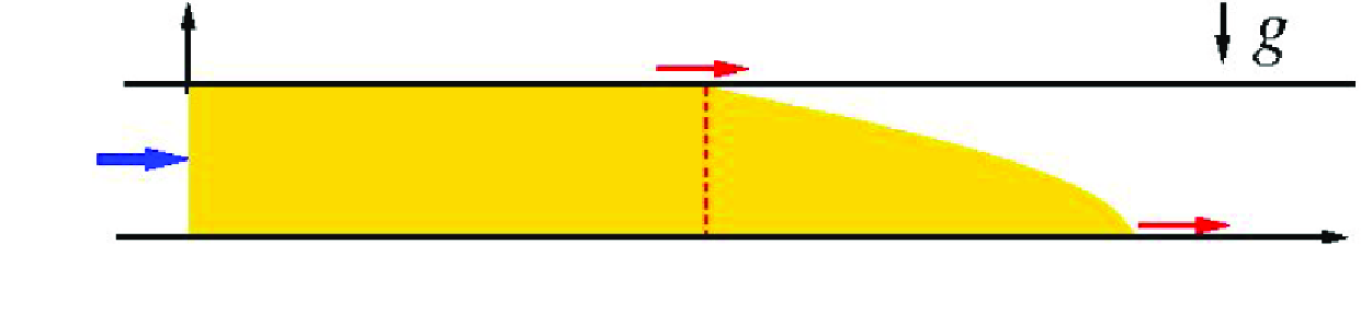The interpretation of the driving buoyancy mechanism is as follows: the hydrostatic pressure fields $p_j \propto - \rho _j g z$ produce a horizontal pressure gradient $\propto g^{\prime} = |\rho _{c}/\rho _{a} - 1| g$ , where $g$ is the gravitational acceleration, $z$ is the vertical upward coordinate, $j=a,c$ , and $g^{\prime}$ is the reduced gravity. The buoyancy is balanced by inertial or viscous effects, depending on the parameters of the system, in particular, if the Reynolds number is large or small. Here, we focus attention on the so-called viscous GC, dominated by a buoyancy–viscous dynamic balance (small Reynolds number); the motion is confined in a horizontal gap, and sustained by a source, as sketched in figure 1.

Viscous GCs have numerous applications in nature and industry. The systems of interest belong to various prototypes, such as Newtonian or non-Newtonian fluids, two-dimensional (2-D) or cylindrical axisymmetric (AXI) propagation, fixed or time varying (influxed) volume, and liquid or porous medium. An important distinction is between the unconfined and confined (gap) domain into which the GC propagates. Geostrophic and environmental GCs are often unconfined (e.g. spread of lava or oilspills), and have received significant attention. The confined GC occurs often in a gap where one viscous fluid displaces another viscous fluid particular in the context of porous layers (e.g. Taghavi et al. 2009;Ciriello & Di Federico 2013; Zheng, Rongy & Stone 2015; Hinton 2020 and the review by Zheng & Stone (2022)). A less investigated type of confined viscous GC occurs when the injected fluid encounters no friction from the displaced fluid (e.g. oil injected into air). A typical application of this type of GC is injection moulding (Hoffman 2014); in this process, the fluid viscosity is typically approximated by a power law. Our paper attempts to close some gaps of knowledge concerning the flow of viscous GCs confined by a top, such as the following. What are the convenient scalings and governing parameters? When are self-similar solutions available? What are the differences between two-dimensional and axisymmetric flows? What is the behaviour at the transition from unconfined to confined flows? These clarifications will be sought for Newtonian and power-law viscous fluids.

Figure 1. Sketch of the confined system. The volume (per unit width) is $\mathcal {V} = q t^\alpha$ . In the self-similar flow, $x_G = y_G K t^\beta$ , $x_N= K t^\beta$ and $y_G$ depends on the parameter $J$ . In the axisymmetric geometry, $r$ replaces $x$ and $\mathcal {V}$ is per radian. $\alpha , \beta , K, y_G$ are constants.

The flow studied here is sketched in figure 1. Consider the two-dimensional propagation of a viscous fluid injected into a small gap of height $H$ between two horizontal plates. This is a simplification of a rectangular channel of width $\gg H$ . Assume that the ambient fluid, displaced from the gap by the injected fluid, is less dense and significantly less viscous than the injected one (e.g. oil injected into air). In this case, the following type of flow may appear: the dense fluid forms a slug which fills the gap in $0\lt x \leqslant x_G(t)$ , while the fluid ahead of the slug, in $x_G(t) \lt x \leqslant x_N(t)$ , forms a viscous GC with an inclined interface. The subscripts $G$ and $N$ denote the ‘grounding line’ and the nose of the GC. Moreover, such flows may be self-similar, in the sense that the slug and GC elongate while maintaining a constant length ratio. The relevant questions are the following. When is the flow ‘confined’ and when can it be considered free (after all, the unconfined flow also propagates in some gap)? When is the flow self-similar? What is the solution? What is the connection between the theories of the unconfined and confined GCs? In this context, we note that the thin-layer (lubrication) theory for the unconfined viscous GCs of volume $q t^\alpha$ provides a rigorous similarity solution for arbitrary $\alpha \geqslant 0$ , for 2-D and AXI geometries, for Newtonian and power-law fluids (Huppert 1982; Di Federico, Malavasi & Cintoli 2006; Sayag & Worster 2013; Ungarish 2020); the propagation $\sim t^\beta$ and the height profile can be calculated analytically.

The forerunner of this study (including additional background material) is the work of Hutchinson, Gusinow & Grae Worster (2023), referred below as HGW, which considered the flow sketched in figure 1 in axisymmetric geometry, with the source at the origin. HGW assume a volume $\mathcal {V}= q t$ (per radian) and show that for a Newtonian fluid, a self-similar flow with propagation $r_N = K t^{1/2}$ is predicted in the lubrication-theory framework. In scaled form, the only parameter of this flow is $J$ , roughly the ratio of the typical thickness $l$ of an unconfined GC to $H$ . The ratio between the length of the slug (position of the grounding line), $r_G$ , to $r_N$ is a constant $y_G$ . The values of $K$ and $y_G$ depend only on $J$ and can be obtained by the integration of a second-order ordinary differential equation (ODE), which combines continuity with the dynamic buoyancy–shear balance. Essential to this solution are the boundary conditions at the nose of the GC and at the grounding line. The theoretical predictions have been verified against experiments, with satisfactory agreement. The obvious question, which has motivated the present work, is if this type of confined self-similar flow is present in other systems. Here, we show that the HGW solution can be extended to two-dimensional flows and to power-law viscous fluids.

The justification of this extension is both of academic interest and application. The new results are expected to improve our understanding of, and modelling tools for, the flow of viscous GCs in the confined situation. The practical aspect of this study is provided by the observation of Hoffman (2014) that gravity may play a significant role in the injection moulding industry. This is consistent with the sketch in figure 1: the front portion of the injected material is expected to be a gravity current. Since moulds are not necessarily axisymmetric and typically non-Newtonian (power-law), the present extension of the work HGW is expected to be beneficial.

We show that confined self-similar flows appear for select values of $\alpha$ , depending on the geometry and on the behaviour index $n$ of the power-law shear. The propagation is like $K t ^ \beta$ , and $\beta$ is equal to $\alpha$ for two-dimensional flows and $(1/2) \alpha$ for axisymmetric flows. For all cases, $J$ and $K$ increase with $y_G$ , and there is a value $J_0$ below which the GC behaves as in the unconfined case. The transition is elucidated.

The paper is organised as follows. We first consider Newtonian flows because this facilitates the understanding of the mathematical framework and physical effects. In § 2, we analyse the two-dimensional (referred to as 2-D) flow and demonstrate that similarity solutions exist for $\alpha = 1/2$ only (i.e. $\mathcal {V} = q t^{{1/2}}$ ), while $x_N = Kt^{1/2}$ . In a properly scaled form, the only parameter that fixes the values of $y_G$ and $K$ is $J$ (conversely, a given $y_G$ determines $J$ and $K$ of the system). We obtain the solution (for all the domain of $y_G$ ) by a single numerical integration of an ODE, and also by an analytical approximation, which turns out to be very accurate. In § 3, we briefly extend the analysis to the axisymmetric geometry, where $\alpha = 1$ and $r_N = K t^{1/2}$ . This is a revisit of the flow considered by HGW; we show that the same results are obtained by a simpler and more insightful method, improve the accuracy of the approximated solution, and also clarify the transition to the non-confined system. The investigation is extended to power-law viscous fluids in § 4 and concluding remarks are presented in § 5. The derivation of the typical length of a unconfined GC is given in the Appendix.

2. The rectangular configuration (2-D)

We are concerned with a particular case of power-law influxed volume, $\mathcal {V} = q t^\alpha$ , and propagation, $x_N = K t^\beta$ . Details of the analysis for unconfined GCs of this type are given in § 14 of Ungarish (2020) and the references therein. Here, we focus attention on the system in which the influxed fluid is confined by a gap of height $H$ starting from the source. In the 2-D case and Newtonian fluid, the solution requires $\alpha = 1/2, \beta = 1/2$ . Here, we use these values, but in some equations during the derivation, we shall also mention the more general form with $\alpha$ and $\beta$ . This will facilitate the understanding why only these particular values are compatible with the confinement constraint.

The densities of the ambient and dense (current) fluids are $\rho _{c}$ and $\rho _{a} (\lt \rho _{c})$ , and the reduced gravity is $g^{\prime} = (1-\rho _{a}/\rho _{c}) g$ . We neglect the viscosity of the ambient fluid, which usually implies a very small $\rho _{a}/\rho _{c}$ (e.g. oil in air) and hence $g^{\prime} = g$ . This detail is unimportant to our analysis. We also neglect surface tension effects.

The standard lubrication-theory simplifications are used for the GC. The governing dynamic balance for the horizontal velocity $u(x,z,t)$ is between the buoyancy-driving and viscous shear

(2.1) \begin{equation} 0 = - g^{\prime} \frac {\partial h}{\partial x} + \nu \frac {\partial ^2 u}{\partial z^2}. \end{equation}

Integration, subject to the boundary condition of no-slip at the bottom $z=0$ and no-shear at the interface $z=h(x,t)$ yields $u(x,z,t)$ . The convenient variable for the GC analysis is the depth-averaged velocity (dimensional)

(2.2) \begin{equation} \bar {u}(x,t) = \frac {1}{h} \int _0^h u(x,z,t) {\rm d}z = - \frac {g^{\prime}}{3 \nu } h^2 \frac {\partial h}{\partial x}. \end{equation}

We switch to dimensionless variables. The horizontal and vertical lengths are scaled with $H$ . Volume (per width) is scaled with $H^2$ . The velocity and time are scaled with

(2.3) \begin{equation} U=\frac {g^{\prime}}{3 \nu }H^2, \quad T= \frac {H}{U}, \end{equation}

and the volume flux coefficient, $q$ , is scaled with

(2.4) \begin{equation} Q = H^2/T^\alpha = H^2/ T^{1/2} = (H^3 U)^{1/2} = H^{5/2} \left ( \frac {g^{\prime}}{3 \nu } \right ) ^{{1/2}}. \end{equation}

Subsequently, in this section, unless stated otherwise, the variables $x, t, h, u, \mathcal {V}$ and $q$ are dimensionless, scaled as defined above. The dimensional counterpart, when needed, will be denoted by an asterisk; in particular, we note that the dimensional flux coefficient, which will appear in the definition of $J$ , is denoted $q^\ast$ .

An inspection of the scaled balances reveals that the dimensionless $q$ is the only input parameter of the problem. However, the value of the coefficient $q$ lacks a clear-cut physical connection with the confinement effect. HGW suggested the more convenient parameter $J = l/H$ , where $l$ is the typical length of the free (unconfined) GC with the same dimensional volume $q^\ast \cdot (t^\ast )^{1/2}$ . Note that $Q \propto H^{5/2}$ , see (2.4), and this suggests

(2.5) \begin{equation} J = q^{2/5} = \left ( \frac {3 \nu q^{\ast 2}}{g^{\prime}} \right )^{1/5} / H . \end{equation}

(Again, the asterisk is used to distinguish between the dimensional and the dimensionless coefficients $q$ .) The right-hand side of (2.5) is clearly a ratio of a length $l$ to $H$ . As expected, $l$ can be regarded as the typical length scale (thickness) of the unconfined GC, see the Appendix. Therefore, the value of $J = q^{2/5}$ is expected to be a measure of the importance of the confinement. We keep in mind that $q \propto J$ , i.e. a stronger influx will be more affected by the boundaries of the gap. However, a weak influx (very small $J$ ) is expected to produce a thin GC over the bottom of the gap, and be unaffected by the confinement. This will be clarified and quantified later.

Using the standard lubrication simplification, the depth-averaged velocity of the GC is

(2.6) \begin{equation} \bar {u}(x,t) = - h^2 \frac {\partial h}{\partial x}. \end{equation}

The continuity equation of the GC reads

(2.7) \begin{equation} \frac {\partial h}{\partial t}+ \frac {\partial }{\partial x} (h \bar {u}) = 0, \quad \text {i.e.} \quad \frac {\partial h}{\partial t} - \frac {\partial }{\partial x} \left ( h^3\frac {\partial h}{\partial x} \right ) = 0. \end{equation}

We emphasise that (2.6) and (2.7) are valid for $x_G(t) \leqslant x \leqslant x_N(t)$ . In the slug $0 \leqslant x \leqslant x_G(t)$ , we impose $h=1$ .

The boundary conditions at $x_N(t)$ are $h_N =0$ , while $u_N = {\rm d} x_N /{\rm d}t$ . The last condition implies a finite negative $[h^2 (\partial h / \partial x)]_N$ (for more details, see Ungarish (2020) §14.1).

The boundary conditions at the grounding line $x_G(t)$ are the obvious $h_G = 1$ and total volume conservation

(2.8) \begin{equation} \mathcal {V} = \int _0^{x_N(t)} h(x,t) {\rm d}x = x_G(t) + \int _{x_G(t)}^{x_N(t)} h(x,t) {\rm d}x = q t^{1/2} \ (= qt^\alpha ). \end{equation}

We apply $t$ derivative to the balance (2.8), use (2.7) to eliminate $\partial h /\partial t$ and recall $h_G = 1, h_N =0$ . We obtain the condition

(2.9) \begin{equation} - h_G^3 \left [ \frac {\partial h}{\partial x} \right ]_G = \frac {1}{2} q t ^{-{1/2}} \ ( = \alpha qt ^{\alpha - 1}) , \end{equation}

which can be simplified because $h_G = 1$ . We observe that this is a flux condition which, in general for the 2-D geometry, can be expressed as

(2.10) \begin{equation} (h \bar {u})_G = \alpha q t^{\alpha - 1}. \end{equation}

Since $h_G =1$ , this is actually a condition for $\bar {u}_G$ .

Introduce the reduced space coordinate of the GC:

(2.11) \begin{equation} y=x/x_N(t) \quad (0 \leqslant y \leqslant 1) . \end{equation}

We obtain from (2.6) and (2.7) the following equation for $\bar {u}(y,t)$ and $h(y,t)$ of the GC:

(2.12) \begin{equation} \bar {u}(y,t) = - h^2 \frac {1}{x_N}\frac {\partial h}{\partial y}, \end{equation}

(2.13) \begin{equation} \frac {\partial h}{\partial t} - y \frac {\dot {x}_N}{x_N} \frac {\partial h}{\partial y} - \frac {1}{x^2_N} \frac {\partial }{\partial y} \left ( h^3 \frac {\partial h}{\partial y} \right ) =0, \end{equation}

where the upper dot denotes $t$ derivative. The conditions at the leading edge $y=1$ are $h = 0$ and $\bar {u} = \dot {x}_N$ . The conditions at $y_G$ are, again, $h_G = 1$ , while (2.9) is expressed as

(2.14) \begin{equation} - \left [ \frac {\partial h}{\partial y} \right ]_G = \frac {1}{2} q t ^{-{1/2}} x_N(t) \ ( \ = \alpha q t^{\alpha -1} x_N(t) \ ) . \end{equation}

2.1. Similarity solution

It is insightful to start the similarity analysis with the GC of volume $\mathcal {V} = q t^\alpha$ , where $\alpha \geqslant 0$ is a constant. We shall show that, while such solutions are valid in general for unconfined GCs, the confinement imposes the restriction $\alpha = 1/2$ .

We seek a similarity solution of the form

(2.15) \begin{equation} x_N = {K} t ^\beta , \quad h=\frac {\mathcal {V}}{x_N}\mathcal {H}(y)= \frac {q}{K} t^{\alpha - \beta } \mathcal {H}(y); \quad \bar {u} = \beta K t^{\beta - 1} \mathcal {U}(y), \end{equation}

where $K$ and $\beta$ are some positive constants, and $\mathcal {U}(1) = 1$ . Substitution into (2.12) yields

(2.16) \begin{equation} \beta = \frac {3 \alpha + 1}{5}. \end{equation}

The condition $h = 1$ at $y_G$ for all $t$ implies that $\partial h(y,t)/ \partial t = 0$ , i.e. $h = h(y)$ . This can be satisfied when $\beta = \alpha$ , see (2.15), and next, (2.16) yields $\beta = \alpha =1/2$ . This is the justification for the system under consideration here: a consistent matching between a confined slug and a leading free 2-D GC for a Newtonian fluid is possible only when $\mathcal {V} = q t^{1/2}$ . Note that the term $t^{\alpha -1} x_N(t) = K t^{\alpha + \beta -1}$ on the right-hand side of (2.14) is now a constant, consistent with the left-hand side.

We shall proceed by letting

(2.17) \begin{equation} x_N = K t^{1/2}, \quad h(y,t) = h(y) = K^{2/3} \lambda (y), \quad \bar {u}(y,t) = - \lambda ^2 \lambda ^{\prime} K t ^{-{1/2}}, \end{equation}

where the prime denotes $y$ derivative. The variable $\lambda (y)$ represents the thickness of the GC. The rescaling of $h(y)$ simplifies the manipulation and solution of the continuity equation, as seen later. Note that we replaced $\mathcal {U}(y)$ by $-\lambda ^2(y) \lambda ^{\prime} (y)/\beta$ , in accord with (2.12). The task is to calculate $\lambda (y)$ , $K$ and $y_G$ for a given $J$ .

The substitution of (2.17) into (2.13) yields

(2.18) \begin{equation} (\lambda ^3\lambda ^{\prime})^{\prime}+ \frac {1}{2} y \lambda ^{\prime} = 0, \end{equation}

with the boundary conditions $\lambda (1)=0$ and $-\lambda ^2 \lambda ^{\prime} = 1/2 \ ( = \beta )$ at $y=1$ . The last condition follows from $\bar {u}(y=1, t) = \dot {x}_N(t)$ (or $\mathcal {U}(1) = 1$ ). In other words, we require that $y=1$ is a singular-regular point of (2.18). Equation (2.18) and the boundary conditions at $y=1$ turn out to be the generic governing equations for the viscous GC in the unconfined geometry for $\alpha = \beta = 1/2$ (see Ungarish 2020). The reason is that these formulae reproduce the balances for the GC before the confinement conditions are applied.

Using a Frobenius series expansion $\lambda = \xi ^\gamma (a_0+a_1\xi +\cdots )$ , where $\xi =(1-y)$ , we obtain the solution

(2.19) \begin{equation} \lambda (y)={\left [ \frac {3}{2} \right ]}^{1/3}{(1-y)}^{{1}/{3}}\left [ 1 - \frac {1}{24} (1-y) - \frac {1}{4032} (1-y)^2 + O[(1-y)^3]\right ]. \end{equation}

We can verify that the boundary conditions at $y=1$ are satisfied. This result is in agreement with the solution of Huppert (1982) for the unconfined GC (after correction of a misprint in the coefficient of the second term).

We use this approximation to obtain regular boundary conditions for $\lambda$ and $\lambda ^{\prime}$ at $y = 1-\varDelta$ , where $\varDelta$ is some convenient small interval, say $10^{-3}$ . Then, the numerical integration of (2.18) can be performed by a standard method. (We used a fourth-order Runge–Kutta). We obtain $\lambda (y)$ and $\lambda ^{\prime}(y)$ at a large number of gridpoints for the $y \in [0, 1)$ interval.

The conclusion is that the calculation of $\lambda (y)$ is decoupled from the calculation of $K$ and $y_G$ . This is the consequence of the rescaling of $h(y)$ in (2.17). We argue that the one-time integration of (2.18) for $y$ from $1$ to $0$ is sufficient for closing the similarity flow solution in the confined geometry, as follows.

2.2. Calculation of $J$ and $K$

The solution $\lambda (y)$ provides a universal height profile for GCs of volume $\propto t^{1/2}$ , which propagate like $K t^{1/2}$ , where $K$ is as yet an unspecified constant. The implementation to a specific system requires the use of the parameter $J$ , see (2.5), and the calculation of the corresponding coefficient $K$ . Physically, the confinement conditions must be applied.

We recall the confinement conditions $h_G = 1$ and (2.14), which now read

(2.20) \begin{equation} K^{2/3} \lambda (y_G) = 1, \quad - K ^{2/3} \lambda ^{\prime} (y_G) = \frac {1}{2} q K, \end{equation}

and can be rewritten as

(2.21) \begin{equation} q = - 2 \lambda ^{1/2} \lambda ^{\prime}, \quad K = 1/\lambda ^{3/2} \quad \text {at}\;y = y_G. \end{equation}

Recall that we have obtained the values of $\lambda$ and $\lambda ^{\prime}$ at $y \in [0,1]$ . Any point $y$ of the solution can be regarded as $y_G$ . For this point, (2.21) produces $q$ and $K$ of the respective confined GC. In other words, the numerical solution of (2.18) with the boundary conditions at $y=1$ , provides (implicitly) the values of $y_G$ and $K$ for any plausible $q$ (or $J = q^{2/5}$ ).

Figure 2. Results of numerical integration of (2.18) and use of (2.21). Two-dimensional, $\mathcal {V} = q t^{1/2}$ , $x_N = K t^{1/2}, \ h = K^{2/3} \lambda (y), \ \bar {u} = (1/2)K t^ {-{1/2}} \mathcal {U}(y)$ . The value of $J$ determines the grounding-line position $y_G$ and the coefficient $K$ (panel c).

Typical results are shown in figure 2. In the upper frames, we see the scaled thickness profile $\lambda (y)$ ( $= h(y)/K^{2/3}$ ) and the profile $\mathcal {U}(y) = -2 \lambda ^2 \lambda ^{\prime}$ . This is the generic behaviour of the unconfined GC with influxed volume $\mathcal {V} = q t ^{1/2}$ , i.e. for $\alpha = {1/2}$ . In the confined GC, the profiles $\lambda (y)$ and $\mathcal {U}(y)$ are relevant for $y_G \leqslant y \leqslant 1$ (the flow in the confined part $y\lt y_G$ can be represented by the horizontal lines $\lambda (y_G)$ and $\mathcal {U}(y_G)$ ). The lower frame provides the coefficients of propagation for a confined flow: for a given $y_G$ , the plot provides the values of $J$ and $K$ ; conversely, for a given parameter $J$ , the plot provides the values of $y_G$ and $K$ . This closes the description of the propagation pattern. We see that for a large $J = l/H$ , the grounding line position $y_G$ approaches 1, i.e. most of the influxed fluid fills the gap. The full-length unconfined GC needs a wider space ( $h\gt 1$ ) than the available gap and, hence, only a short part $y \in [y_G,1]$ where $h \leqslant 1$ appears. However, when $J$ is close to 1, the interface of the unbounded GC barely touches the upper boundary of the gap and, hence, $y_G$ is small. For $J\lt 0.85 = J_0$ , the GC will not touch the upper boundary. This is the limit of applicability of the confined GC theory; for smaller $J$ (weaker influx), $y_G$ is irrelevant. In this case, we return to the theory of the classical unconfined GC. The profiles $\lambda$ and $\mathcal {U}$ remain valid, but the value of $K$ must be determined by a different condition, not by (2.21); see § 2.3 and Ungarish (2020).

Since $J$ and $K$ are increasing function of $y_G$ , it is convenient to introduce the parameters $J_0, K_0$ and $J_{0.9},K_{0.9}$ , which correspond to the situations $y_G=0$ and $y_G=0.9$ , respectively. For $J\lt J_0$ , the GC is unconfined and propagates with $K \lt K_0$ . For $J\gt J_{0.9}$ , the GC is a small part of the influxed volume and the propagation is with $K\gt K_{0.9}$ . The values of the present system are tabulated in table 1.

Table 1. Two-dimensional, the effect of $n$ on the values of $\alpha , \beta , J_0, K_0, J_{0.9}, K_{0.9}$ and $\kappa$ .

Interestingly, the comparison between the numerical $\lambda (y)$ and the two-term Frobenius series solution (2.19) reveals a remarkable agreement, of three to four significant digits, over the entire range of $y$ . This could be anticipated, because the coefficient of the $(1-y)^3$ term is $2.5\times 10^{-4}$ . The conclusion is that the analytical two-terms $\lambda$ is a very reliable tool for the calculation of the entire flow, in particular, for the prediction of $J$ and $K$ . In the present case, the numerical solution $\lambda (y)$ is needed mostly for support, not for the predictions.

The Frobenius series solution provides the following results. The first term gives

(2.22) \begin{equation} J \approx J^{(1)} = \left [ \frac {2}{3 (1 - y_G)} \right ] ^{1/5}, \quad K \approx K^{(1)} = \left [ \frac {2}{3 (1 - y_G)} \right ] ^{1/2}. \end{equation}

This slightly overestimates $J$ and underestimates $K$ , by approximately $4\,\%$ for $y_G = 0.5$ , and the accuracy improves as $y_G$ increases. The two-term approximation gives

(2.23a) \begin{equation} J \approx \left [ \frac {23 + y_G}{1 - y_G} \right ] ^{1/5} \left [ \frac {5 +y_G}{36} \right ] ^{2/5} = J^{(1)} \left [ \left ( 1 - \frac {1}{6} (1-y_G) \right ) ^2 \left (1 - \frac {1}{24}(1-y_G) \right ) \right ] ^{1/5}, \end{equation}

(2.23b) \begin{equation} K \approx \left [ \frac {2}{3 (1 - y_G)} \right ] ^{1/2} \left [ 1 - \frac {1}{24} (1-y_G) \right ]^{-3/2} = K^{(1)} \left [ 1 - \frac {1}{24} (1-y_G) \right ]^{-3/2}. \end{equation}

The approximations (2.23) are quite accurate, the difference with the numerical results is less than $0.04\,\%$ in the entire range of $y_G$ . In particular, (2.23a ) shows that for $y_G=0$ , we obtain $J_0 = 0.85$ . The fact that the value is close to 1 confirms the physical meaning of $J$ .

This completes the solution. For a given system (i.e. given $q^*, g^{\prime}, \nu , H$ ), we calculate the scalings $U, T$ and $Q$ and the parameter $J$ by (2.5). Figure 2 provides the appropriate values of $y_G$ and $K$ . The grounding line and nose propagate as $y_G Kt^{1/2}$ and $K t ^{1/2}$ . Conversely, if we wish a certain $y_G$ in our system, the figure provides the necessary $J$ and value of $K$ . We may adjust the values of $q^\ast$ , $H$ and $\nu$ for obtaining this $J$ . Note that the slope ${\rm d}J /{\rm d} y_G$ is small in the domain $y_G \lt 0.6$ . This indicates a big sensitivity of $y_G$ on $J$ (ill-conditioned connection). In practice, it may be difficult to obtain (and maintain) a desired value of $y_G$ in this domain.

2.3. Total volume and transition to unconfined flow

The substitution of the similarity variables (2.17) into the global volume conservation (2.8) yields

(2.24) \begin{equation} K \left [ y_G + K^{2/3} \int _{y_G}^1 \lambda (y) {\rm d}y \right ] = q. \end{equation}

We note that in the previous solution for $K$ and $q$ as functions of $y_G$ , we did not impose this condition. The only confinement conditions that we applied is the flux condition (2.21).

We argue that the condition (2.24) is equivalent to the flux condition (2.21). The proof, keeping in mind $\lambda (1) = 0$ ), is as follows. Using integration by parts,

(2.25) \begin{equation} \int _{y_G}^1 \lambda (y) {\rm d}y = - y_G \lambda (y_G) - \int _{y_G}^1 y \lambda ^{\prime} {\rm d}y. \end{equation}

Using (2.18), the integral gives $ -2 \lambda ^3 \lambda ^{\prime}$ at $y=y_G$ . Substitution of $K = 1/\lambda ^{3/2}$ at $y_G$ recovers the first equation of (2.21). In other words, (2.24) and the first equation of (2.21) are alternative ways for obtaining $q= J^{5/2}$ as a function of $y_G$ (in both cases, $K = \lambda _G^{-3/2}$ ). The use of (2.24) requires the integral of $\lambda (y)$ which is easily obtained. The alternative calculations of $q$ versus $J$ can be used as a test of the numerical solution for $\lambda$ .

The connection with the unconfined GC can be formulated. The transition from confined to unconfined occurs when $y_G=0$ in the continuity equation (2.24), and we obtain

(2.26) \begin{equation} K = q^{3/5} / I ^{3/5} = \kappa q^{3/5} = \kappa J^{3/2}, \end{equation}

where

(2.27) \begin{equation} I = \int _{0}^1 \lambda (y) {\rm d}y. \end{equation}

The value of $\kappa$ is given in table 1. We note that (2.24) with $y_G=0$ gives the volume balance for an unconfined GC. Consequently, the result (2.26) expresses the global continuity for the marginally confined ( $y_G=0$ ), but also for the unconfined GC in general, i.e. for $J \leqslant J_0$ systems and, thus, $K \leqslant K_0$ . In these cases, (2.26) replaces (2.21), and the value of $J$ is not a physically relevant parameter of the system, because $H$ does not influence the flow. For the unconfined GC, $H$ is just an arbitrary length scale. In any case, (2.26) yields the following relationship between the unconfined and marginally confined (subscript 0) GCs

(2.28) \begin{equation} K = K_0 (J/J_0)^{3/2} \quad (J \leqslant J_0). \end{equation}

This demonstrates that the confinement enhances the propagation, and the transition about $J_0$ is smooth.

3. Axisymmetric flow (AXI)

In the axisymmetric case, the source is at the axis $r=0$ of a cylindrical coordinate system, while $u$ is in the radial direction. Figure 1, with $r$ replacing $x$ , is relevant. HGW demonstrated that the self-similar confined flow appears for $\mathcal {V} = q t$ volume behaviour, and the propagation is like $K t^{1/2}$ . In other words, this is a $\alpha =1, \beta = 1/2$ case. Here, we briefly derive the solution. We present this derivation because: (a) this allows a clear comparison and contrast with the 2-D case; (b) the present solution is simpler and more insightful than that of HGW; and (c) it facilitates the extension to power-law fluids discussed later.

We start with the observation that the 2-D dynamic result (2.2) for $\bar {u}$ carries over to the AXI case with $r$ replacing $x$ , and the major difference will be in the continuity equation because of the curvature terms.

We switch to dimensionless variables. The horizontal and vertical lengths are scaled with $H$ . Volume (per radian) is scaled with $H^3$ . The velocity and time are scaled with

(3.1) \begin{equation} U=\frac {g^{\prime}}{3 \nu }H^2; \quad T= \frac {H}{U}, \end{equation}

and the flux coefficient $q$ is scaled with

(3.2) \begin{equation} Q = H^3/ T ^\alpha = H^3/ T = H^2 U = H^4 \left ( \frac {g^{\prime}}{3 \nu } \right ). \end{equation}

Subsequently, in this section, unless stated otherwise, the variables $r, t, h, u, \mathcal {V}$ and $q$ are dimensionless scaled as defined above. The dimensional counterpart, when needed, will be denoted by an asterisk; in particular, we note that the dimensional flux coefficient, which will appear in the definition of $J$ , is denoted $q^\ast$ .

Again, the only parameter of the scaled flow in the lubrication-theory approximation is the dimensionless flux coefficient $q$ . It is our intuitive (and correct) understanding that for a weak influx, the GC will be thin and in little contact with the upper boundary, while a strong influx will produce a thick layer that will fill the gap and require a significant pushing pressure. However, the interpretation of the confinement in terms of $q$ is not straightforward. We note that the scaling $Q \propto H^4$ and, hence, the scaled $q \propto H^{-4}$ . This suggests that the major parameter can be defined as

(3.3) \begin{equation} J = q^{1/4} = \left ( \frac { 3 \nu q^\ast }{g^{\prime}} \right )^{1/4} /H. \end{equation}

Here, $q^\ast$ is the dimensional coefficient for the constant-rate influx (per radian; equal to $Q_0/2 \pi$ in the notation of HGW). The right-hand side of (3.3) is clearly a ratio of a length $l$ to $H$ . As indicated, by HGW, this $l$ can be regarded as the typical length scale (thickness) of the unconfined GC, see the Appendix. Therefore, $J = q^{1/4}$ is expected to represent the importance of the confinement.

The depth-averaged radial velocity is

(3.4) \begin{equation} \bar {u}(r,t) = - h^2 \frac {\partial h}{\partial r}. \end{equation}

The continuity equation takes into account the divergent geometry and reads

(3.5) \begin{equation} \frac {\partial h}{\partial t}+ \frac {1}{r}\frac {\partial }{\partial r} \left ( r h \bar {u} \right ) = 0, \quad \text {i.e.} \quad \frac {\partial h}{\partial t}-\frac {1}{r}\frac {\partial }{\partial r} \left ( r h^3\frac {\partial h}{\partial r} \right ) = 0. \end{equation}

Again, (3.4) and (3.5) are valid in the GC in the domain $r_G(t) \leqslant r \leqslant r_N(t)$ . In the slug, $0 \leqslant r \leqslant r_G(t)$ , the confinement imposes $h=1$ .

The boundary conditions at $r_N(t)$ are $h_N =0$ , while $\bar {u}_N= {\rm d} r_N/{\rm d}t$ . The boundary conditions at the grounding line $r_G(t)$ are the obvious $h_G = 1$ , and the total volume conservation (per radian) reads

(3.6) \begin{equation} \mathcal {V} = \frac {1}{2} r_G^2 + \int _{r_G(t)}^{r_N(t)} h(r,t) r {\rm d}r = q t \ (= q t^ \alpha \ ). \end{equation}

(Again, the specific result on the right-hand side is for $\alpha = 1$ , but we also add the formal expression for a general $\alpha$ . This will facilitate the justification that the similarity solution with confinement conditions requires $\alpha = 1$ .) We apply $t$ derivative to (3.6) and use (3.5) to eliminate $\partial h/\partial t$ . We obtain the condition

(3.7) \begin{equation} - r_G h_G^3 \left [ \frac {\partial h}{\partial r} \right ]_G = q = \ (= \alpha q t^{\alpha - 1} \ ), \end{equation}

which can be simplified because $h_G = 1$ . We observe that this is a flux condition which, in general for the axisymmetric geometry, can be expressed as

(3.8) \begin{equation} (r h \bar {u})_G = \alpha q t^{\alpha - 1}. \end{equation}

Introduce

(3.9) \begin{equation} y=r/r_N(t) \quad (0 \leqslant y \leqslant 1). \end{equation}

We obtain from (3.4) and (3.5) the following equations for $\bar {u}(y,t)$ and $h(y,t)$ of the GC:

(3.10) \begin{equation} \bar {u}(y,t) = - h^2 \frac {1}{r_N}\frac {\partial h}{\partial y}, \end{equation}

(3.11) \begin{equation} \frac {\partial h}{\partial t} - y \frac {\dot {r}_N}{r_N}\frac {\partial h}{\partial y} - \frac {1}{r^2_N}\frac {1}{y}\frac {\partial }{\partial y} \left ( yh^3\frac {\partial h}{\partial y} \right ) =0, \end{equation}

where the upper dot denotes $t$ derivative. The conditions at the leading edge $y=1$ are $h = 0$ and a $\bar {u} = \dot {r}_N$ .

The conditions of confinement and the ‘grounding line’ are

(3.12) \begin{equation} h = 1 \quad 0 \leqslant y \leqslant y_G, \end{equation}

(3.13) \begin{equation} - y_G (h_G^3) \left ( \frac {\partial h}{\partial y} \right )_G = q \ (= \alpha q t^{\alpha - 1} \ ) . \end{equation}

Note that the last equation can be simplified because $h_G = 1$ .

3.1. Similarity solution

Again, we start the similarity analysis with the case $\mathcal {V} = q t^\alpha$ where $\alpha \geqslant 0$ is a constant. We shall show that the confinement imposes the restriction $\alpha = 1$ .

We seek a similarity solution of the form

(3.14) \begin{equation} r_N = {K} t ^\beta ; \quad h=\frac {\mathcal {V}}{r^2_N}\mathcal {H}(y)= \frac {q}{K^2} t^{\alpha - 2\beta } \mathcal {H}(y), \quad \bar {u} = \beta Kt^{\beta -1} \mathcal {U}(y), \end{equation}

where $K$ and $\beta$ are some positive constants and $\mathcal {U}(1) = 1$ . Substitution into (3.10) yields

(3.15) \begin{equation} \beta = \frac {3 \alpha + 1}{8}. \end{equation}

The argument used in the 2-D case is relevant: the boundary condition $h=1$ at the position $y_G$ for all $t$ implies $\partial h(y,t)/ \partial t =0$ , i.e. $h = h(y)$ . This can be satisfied when $\beta = \alpha /2$ , see (3.14), and next, (3.15) yields $\alpha = 1, \beta =1/2$ . This is the justification for the system solved by HGW: a consistent matching between a confined slug and a leading free axisymmetric GC for a Newtonian fluid is possible only for the $\mathcal {V} = q t$ case. Note that the right-hand side of (3.13) is consistent with the left-hand side only for $\alpha = 1$ .

We shall proceed letting

(3.16) \begin{equation} r_N = K t^{1/2}, \quad h(y,t) = h(y) = K^{2/3} \lambda (y), \quad \bar {u}(y,t) = - \lambda ^2 \lambda ^{\prime} K t ^{-{1/2}}, \end{equation}

where the prime denotes $y$ derivative. The variable $\lambda (y)$ represents the thickness of the GC. The rescaling of $h(y)$ simplifies the manipulation and solution of the continuity equation, as seen later. Again, we replaced $\mathcal {U}(y)$ by $-\lambda ^2(y) \lambda^{\prime} (y)/\beta$ , in accord with (3.10). Substitution of (3.16) into (3.11) yields

(3.17) \begin{equation} (y\lambda ^3\lambda ^{\prime})^{\prime}+ \frac {1}{2} y^2 \lambda ^{\prime} = 0. \end{equation}

The boundary conditions for this equation are $\lambda (1)=0$ and $-\lambda ^2 \lambda ^{\prime}= \beta = 1/2$ . The justification is like in the 2-D counterpart, and we require that $y=1$ is a singular-regular point of (3.17).

It turns out that (3.17) and the boundary conditions at $y=1$ are the generic formulation for the viscous GC in the unconfined geometry for $\alpha =1, \beta = 1/2$ (see Ungarish 2020). This is not surprising, because these are the balances of a GC over a solid bottom before the application of the confinement conditions.

Using a Frobenius series expansion $\lambda = \xi ^\gamma (a_0+a_1\xi +\cdots )$ , where $\xi =(1-y)$ , we obtain

(3.18) \begin{equation} \lambda (y)={\left [ \frac {3}{2} \right ]}^{1/3}{(1-y)}^{{1}/{3}}\left [ 1 + \frac {1}{12} (1-y) + \frac {59}{1008} (1-y)^2 + O[(1-y)^3]\right ]. \end{equation}

This result is in agreement with the solution of Huppert (1982) for the axisymmetric unconfined GC (after correction of a misprint in the coefficient of the second term). We use this approximation to obtain regular boundary conditions for $\lambda$ and $\lambda ^{\prime}$ at $y = 1-\varDelta$ , where $\varDelta$ is some convenient small interval, say $10^{-3}$ . Then, the numerical integration of (3.17) can be performed by a standard method. (We used a fourth-order Runge–Kutta). We obtain $\lambda (y)$ and $\lambda ^{\prime}(y)$ at a large number of gridpoints for the $y \in (0, 1)$ interval. This one-time integration of (3.17) is sufficient for closing the similarity flow solution for the confined flow, as follows.

3.2. Calculation of $J$ and $K$

An important point of the present formulation is that the calculation of $\lambda (y)$ is generic, independent of the value of $y_G$ , and decoupled from the calculation of $K$ and $J$ . Actually, $J$ and $K$ are by-products of the solution of the generic (or universal) equation for $\lambda$ of the unconfined GC, when $y_G$ is imposed. We emphasise this insight because it provides a significant simplification over the method used by HGW for solving the same problem. The $\lambda (y)$ (thickness, or height) profile of the unconfined GC is determined by the conditions at the nose $y=1$ , in particular, $\lambda = 0$ . Looking back from this point, the confined GC obeys the same balances (and hence admits the same solution $\lambda$ ) until the thickness, which grows as $y$ decreases, encounters the upper boundary at $y_G$ . Suppose we have the values of $\lambda$ and $\lambda ^{\prime}$ at $y$ . Any point $y$ of the solution can be regarded as $y_G$ . In view of the boundary conditions (3.12) and (3.13), for $y=y_G$ , we calculate

(3.19) \begin{equation} J= q^{1/4} = [- y \lambda ^{\prime}(y)/\lambda (y)] ^{1/4}, \quad K = 1/ [\lambda (y)] ^{3/2}. \end{equation}

Thus, the use of the numerical solution for obtaining $J$ and $K$ as functions of $y_G$ , or $y_G$ as a function of $J$ , is straightforward. Results are shown in figure 3. The physical behaviour is like in the 2-D case. For $J \gt 1$ , the grounding line $y_G$ is close to the nose, and for $J \lt 0.55 \approx J_0$ , the GC can be considered unconfined. In the AXI system, the value of $J_0$ is less clear-cut than in the 2-D case, because $\lambda$ is unbounded at $y=0$ . Formally, the interface of the axisymmetric influxed GC will intersect the upper boundary of any finite gap, but this is unrealistic because a very large $\mathcal {U}$ is needed at small $y$ , see figure 3. It makes sense to introduce some artificial $y_{min }$ (0.05 say) as a mimic of the radius of a realistic source and consider GCs with $y_G \leqslant y_{min }$ as unconfined. This is consistent with the estimate $J_0= 0.55$ . Like in the 2-D case, it is convenient to consider the parameters $J_0,K_0$ and $J_{0.9}, K_{0.9}$ , see table 2, whose meaning is unchanged by the geometry.

Figure 3. Results of numerical integration of (3.17) and use of (3.19). AXI, $\mathcal {V} = q t$ , $r_N = K t^{1/2}, \ h = K^{2/3} \lambda (y), \ \bar {u} = (1/2)K t^ {-{1/2}} \mathcal {U}(y)$ . The value of $J$ determines the grounding-line position $y_G$ and the coefficient $K$ (panel c). For comparison with HGW, recall $y_G = \eta _G/\eta _N$ and $K = \eta _N$ .

Table 2. AXI, the effect of $n$ on the values of $\alpha , \beta , J_0, K_0, J_{0.9}, K_{0.9}$ and $\kappa$ .

The analytical $\lambda (y)$ series (3.18) is also convenient for an approximate calculation of $K$ and $J$ by (3.19). (The identity $\lambda ^{\prime}/\lambda = (\ln \lambda ) ^{\prime}$ is useful). Using the first two terms, we obtain

(3.20) \begin{equation} K \approx \left ( \frac {2}{3} \frac {1}{1-y_G } \right )^{1/2} \left [ 1 + \frac {1}{12} (1-y_G) \right ] ^{-3/2}, \end{equation}

(3.21) \begin{equation} J^4 \approx y_G \left ( \frac {1}{3} \frac {1}{1-y_G} + \frac {1}{13 - y_G} \right ). \end{equation}

This demonstrates that $J$ is large for $y_G$ very close to 1. However, for $y_G = 0.95$ , we obtain $J \approx 1.59$ (in good agreement with the numerical solution) and for $y_G= 0.5$ , we obtain $J \approx 0.78$ (the numerical solution is $J=0.81$ ). In contrast to the 2-D counterpart, the two-terms approximation is not accurate for $y_G \lt 0.5$ . The reason is that the height (i.e. $\lambda$ ) diverges at the axis. In a realistic system, the source has a finite radius, which is not taken into account by the present solution. Equation (3.17) has a singularity at $y=0$ which defies the Frobenius-series approximation at small $y$ . However, various tests show that the accuracy of the numerical solution is maintained for $y \geqslant 0.05$ , and this is sufficient for the present analysis.

The present method of solution is different from that of HGW. The mathematical model is the same, the parameter $J$ is the same, but the derivation of the similarity solution is different. HGW derived a similarity solution which, in our dimensionless variables, can be expressed as

(3.22) \begin{equation} r_N = \eta _N t^{1/2}, \quad r_G = \eta _G t^{1/2}, \quad h = f(\eta ), \end{equation}

where the similarity variable is $\eta = \eta _N (r/r_N(t))$ and the GC extends from $\eta _G$ to $\eta _N$ (both constants). This means that $\eta _N = K$ , $\eta = K y$ . The governing equation for $f(\eta )$ is identical with our (3.17), the boundary conditions are the same, but the domain of solution is $\eta _G \leqslant \eta \leqslant \eta _N$ (instead of our $y_G \leqslant y \leqslant 1$ ). The main objective was to obtain the coefficients $\eta _N$ and $\eta _G$ as functions of $J$ . To this end, HGW solved the governing equation for $f(\eta )$ numerically for various values of $\eta _N$ (the singularity at $\eta _N$ was resolved using the first term in a Frobenius series corresponding to (3.18)). For each $\eta _N$ , the numerical solution produces the value of $\eta _G$ at which the condition $f =1$ is satisfied. The flux condition $-\eta _G f^3(\eta _G) f^{\prime} (\eta _G) = J^4$ (the equivalent of our first equation in (3.19)) provides the value of $J$ . Evidently, the ratio $ \eta _G/\eta _N$ of HGW corresponds to the present $y_G$ , and the coefficient $\eta _N$ of HGW corresponds to the present $K$ . A comparison of the numerical results $\eta _G/\eta _N$ and $\eta _N$ presented by HGW as functions of $J$ (figure 3 in that paper) shows perfect agreement with our results $y_G$ and $\eta _N$ (figure 3), which were obtained by a considerably smaller effort. This confirms the advantage of the present method of solution, which is the result of a more effective scaling of the similarity variables. However, we emphasise that the physical model and conclusions of HGW are not affected by this simplification.

3.3. Total volume and transition to unconfined flow

Using the similarity variables (3.16), the global volume conservation (3.6) yields

(3.23) \begin{equation} K^2 \left [ \frac {1}{2} y_G^2 + K^{2/3} \int _{y_G}^1 \lambda (y) y {\rm d}y \right ] = q = J^4. \end{equation}

We note that in the previous solution for $K$ and $J$ as functions of $y_G$ , we did not impose this condition. We imposed the flux condition (3.19).

We argue that the condition (3.23) is equivalent to the flux condition at $y_G$ . The proof, keeping in mind $\lambda (1) = 0$ , is as follows. Using integration by parts,

(3.24) \begin{equation} \int _{y_G}^1 \lambda (y) y {\rm d}y = - \frac {1}{2} y^2_G \lambda (y_G) - \int _{y_G}^1 (\frac {1}{2} y^2 \lambda ^{\prime}) {\rm d}y. \end{equation}

Using (3.17), the integral gives $- y \lambda ^3 \lambda ^{\prime}$ at $y=y_G$ .

Some algebra and use of $K = [\lambda (y_G) ]^{-3/2}$ end the proof. Conclusion: the integral condition (3.23) is satisfied by the solution of the generic equation combined with the local flux conditions at $y_G$ . In other words, (3.23) and the first equation of (3.19) are alternative ways for obtaining $q= J^{4}$ as a function of $y_G$ (in both cases, $K = \lambda _G^{-3/2}$ ). The use of (3.23) requires the integral of $y \lambda (y)$ which is easily obtained.

The connection with the unconfined GC can be formulated. Again, since $\lambda$ increases to $\infty$ as $y \to 0$ , we introduce an ad hoc threshold $y_{min }$ (we used $0.05$ , but tests with other small values produced very close results). The GC is considered unconfined if the theoretical $y_G \leqslant y_{min }$ .

The transition from confined to unconfined flows occurs when $y_G=y_{min }$ in the continuity equation (3.23), and we obtain (neglecting small terms)

(3.25) \begin{equation} K = q ^{3/8}/ I ^{3/8} = \kappa q ^{3/8} = \kappa J^{3/2}, \end{equation}

where

(3.26) \begin{equation} I = \int _{y_{min }}^1 \lambda (y) y {\rm d}y. \end{equation}

We note that (3.23) with $y_G=0$ expresses the volume balance of the unconfined GC. Therefore, the result (3.25) is valid for the marginally confined and also for the unconfined GC, i.e. for $J \leqslant J_0$ systems. In these cases, (3.25) replaces (3.19), and the value of $J$ is not a physically relevant parameter of the system, because $H$ does not influence the flow. For the unconfined GC, $H$ is just an arbitrary length scale. The coefficient $\kappa$ in (3.25) is conveniently calculated as a small addition to the numerical solution of $\lambda (y)$ . The value is given in table 2. Since (3.25) is valid for unconfined and marginally confined GC (subscript 0), we obtain the following correlation:

(3.27) \begin{equation} K = K_0 (J/J_0)^{3/2} \quad (J \leqslant J_0). \end{equation}

This demonstrates that the switch from the confined flow to the unconfined $J\lt J_0$ , reduces the speed of propagation. Here, $K$ is continuous and the transition is smooth, as expected.

4. The unified formulation for Newtonian and power-law GCs

In power-law case, the dynamic viscosity of the current is given by

(4.1) \begin{equation} \mu = m \left | \frac {\partial u}{\partial z} \right | ^{n -1}, \end{equation}

where $m$ is the consistency index and $n$ is the behaviour index (or exponent). A fluid is shear-thinning (pseudoplastic) if $n \lt 1$ and shear-thickening (dilatant) if $n \gt 1$ . We define

(4.2) \begin{equation} \nu _{NN} = m/\rho . \end{equation}

The standard fluid is recovered for $n=1$ . In this case, $\nu _{NN} = \nu$ .

Here, we show that the results of the previous sections can be extended, and expressed in a convenient compact form for both Newtonian ( $n = 1$ ) and power-law fluids ( $n \ne 1$ ).

The lubrication theory of the unconfined Newtonian viscous GC (Huppert 1982) has been extended to the general $n$ fluid (see Di Federico et al. 2006; Chowdhury & Testik 2011; Sayag & Worster 2013; Longo et al. 2013; Ungarish 2020 §14.3). Here, we consider the effect of the confinement. We specify the geometry by the dimension $k=2$ (2-D) and $k=3$ (AXI). We denote

(4.3) \begin{equation} \mathcal {G} = g^{\prime}/\nu _{NN}, \end{equation}

keeping in mind that $\nu _{NN} = \nu$ for $n=1$ . The flow is as sketched in figure 1.

The major effect of the power-law behaviour is in the lubrication momentum equation. In a 2-D system with $z$ vertical upward, the balance is

(4.4) \begin{equation} 0 = - g^{\prime} \frac {\partial h}{\partial x} + \nu _{NN}\frac {\partial }{\partial z} \left [ \left | \frac {\partial u}{\partial z} \right | ^{n -1} \frac {\partial u}{\partial z } \right ] . \end{equation}

This equation can be integrated twice with respect to $z$ to obtain $u(x,z,t)$ . The constants of integration are determined again by the same boundary condition as for the Newtonian fluid. We obtain the depth-averaged velocity (dimensional)

(4.5) \begin{equation} \bar {u}(x,t) = \frac {1}{h} \int _0^h u(x,z,t) {\rm d}z = \frac {n}{2n+1} \mathcal {G}^{1/n} \left (- \frac {\partial h}{\partial x} \right )^{1/n} h^{(n+1)/n} . \end{equation}

We switch to dimensionless variables. Lengths are scaled with $H$ and volume (per unit width or per radian) with $H^k$ . The scales for velocity, time and flux coefficient are as follows:

(4.6) \begin{equation} U = \frac {n}{2n +1} \mathcal {G}^{1/n} H ^{(n+1)/n}, \quad T = \frac {H}{U}, \quad Q = \frac {H^k}{T^\alpha } = H^{k + \alpha /n} \left ( \frac {n}{2n +1} \right )^\alpha \mathcal {G}^{\alpha /n}. \end{equation}

Subsequently, in this section, unless stated otherwise, the variables $x, r, t, h, u, \mathcal {V}$ and $q$ are are dimensionless, scaled as defined above. The dimensional counterpart, when needed, will be denoted by an asterisk; in particular, we note that the dimensional flux coefficient, which will appear in the definition of $J$ , is denoted $q^\ast$ .

The insight from the previous Newtonian cases suggests that the convenient parameter for expressing the importance of the confinement of the flow is the dimensionless flux coefficient $q$ at some power. We note that the scaling $Q \propto H^{(k n + \alpha )/n}$ . This suggest the use of the parameter

(4.7) \begin{equation} J = q ^{n/( k n + \alpha )} = \left [ \left ( \frac {2n +1}{n} \right )^\alpha q^\ast \mathcal {G}^{-\alpha /n} \right ]^{n/( k n + \alpha )} \frac {1}{H}. \end{equation}

The right-hand side of (4.7) is the ratio of a length, $l$ , to $H$ . This expresses the ratio of the typical thickness of the unconfined GC to $H$ , see the Appendix.

The dimensionless depth-averaged velocity, for both 2-D ( $\xi = x$ ) and AXI ( $\xi = r$ ) geometries, see (4.5), is

(4.8) \begin{equation} \bar {u}(\xi ,t) = \left (- \frac {\partial h}{\partial \xi } \right )^{1/n} h^{(n+1)/n} . \end{equation}

The continuity equations are

(4.9a) \begin{equation} \frac {\partial h}{\partial t} + \frac {\partial }{\partial x} (h \bar {u}) = 0 \quad \text {(2-D)}, \end{equation}

(4.9b) \begin{equation} \frac {\partial h}{\partial t}+ \frac {1}{r} \frac {\partial }{\partial r} ( r h \bar {u}) = 0 \quad \text {(AXI)}. \end{equation}

The boundary conditions at the nose $\xi _N(t)$ are $h_N =0$ , while $\bar {u}_N = {\rm d} \xi _N /{\rm d}t$ .

The total volume balance is a kinematic consideration. The flux condition results of the analysis of (2.8) and (2.8) carry over to the general power-law fluid. The grounding line conditions are therefore $h_G = 1$ and

(4.10a) \begin{equation} (h \bar {u})_G = \alpha q t^{\alpha - 1} \quad \text {(2-D)}, \end{equation}

(4.10b) \begin{equation} (r h \bar {u})_G = \alpha q t^{\alpha - 1} \quad \text {(AXI)}, \end{equation}

which can be simplified by using $h_G = 1$ . The difference between the Newtonian and power-law fluids appears upon the substitution of (4.8) into (4.9) and (4.10).

The similarity solution is obtained as follows. We define $y = \xi /\xi _N$ , where $\xi$ stands for $x$ or $r$ according to the geometry. We switch to the variables $h(y,t)$ and $\bar {u}(y,t)$ in the domain $y \in [0,1]$ keeping in mind that the grounding line is at $y=y_G\lt 1$ . The governing equations (4.8) and (4.9) for the GC are expressed as

(4.11) \begin{equation} \bar {u}(y,t) = \frac {1}{[\xi _N(t)]^{1/n}} \left (- \frac {\partial h}{\partial y} \right )^{1/n} h^{(n+1)/n} . \end{equation}

(4.12a) \begin{equation} \frac {\partial h}{\partial t} - y \frac {\dot {x}_N}{x_N} \frac {\partial h}{\partial y} - \frac {1}{(x_N)^{(n+1)/n} } \frac {\partial }{\partial y} \left [ h^{(2 n + 1)/n} \left ( - \frac {\partial h}{\partial y} \right ) ^{1/n} \right ] =0 \quad \text {(2-D) }, \end{equation}

(4.12b) \begin{equation} \frac {\partial h}{\partial t} - y \frac {\dot {r}_N}{r_N}\frac {\partial h}{\partial y} - \frac {1}{(r_N)^{(n+1)/n}}\frac {1}{y} \frac {\partial }{\partial y} \left [ y h^{(2 n + 1)/n} \left ( - \frac {\partial h}{\partial y} \right ) ^{1/n} \right ] =0 \quad \text {(AXI}), \end{equation}

where the upper dot denotes $t$ derivative. At the nose $y=1$ , the boundary conditions are $h=0$ and $\bar {u}=\dot {x}_N$ (or $\dot {r}_N$ ). We postulate a self-similar behaviour,

(4.13a) \begin{equation} x_N(t) = K t^\beta , \ \bar {u} = \beta t^{\beta -1} \mathcal {U}(y) , \ h = \frac {\mathcal {V}(t)}{x_N(t)} \mathcal {H}(y) = K^{(n+1)/(n+2)} \lambda (y) t^{\alpha - \beta } \ \ \text {(2-D)}, \end{equation}

(4.13b) \begin{equation} r_N(t) = K t^\beta , \ \bar {u} = \beta t^{\beta -1}\mathcal {U}(y), \ h = \frac {\mathcal {V}(t)}{r^2_N(t)} \mathcal {H}(y) = K^{(n+1)/(n+2)} \lambda (y) t^{\alpha - 2 \beta } \ \text {(AXI)}, \end{equation}

where $\mathcal {U}(1) = 1$ . Here, $\lambda (y)$ is the scaled profile of the height. Such similarity assumptions have been used for the unconfined GC system, see Di Federico et al. (2006); Longo et al. (2013); Sayag & Worster (2013) and Ungarish (2020) §14.3. Substitution into (4.11), (4.12) yields

(4.14) \begin{equation} \beta = \frac {\alpha (n + 2) + n}{2 n + 3} \quad \text {(2-D)}, \quad \beta = \frac {\alpha (n + 2) + n}{3 n + 5} \quad \text {(AXI)} . \end{equation}

With these relationships, we obtain from (4.11)

(4.15) \begin{equation} \bar {u}(y,t) = [-\lambda ^{n+1}(y) \lambda ^{\prime}(y) ]^{1/n} K t^{\beta -1}, \end{equation}

where the prime denotes $y$ derivative. The last equation shows that $\mathcal {U}(y) = [-\lambda ^{n+1} \lambda ^{\prime} ]^{1/n}/\beta$ .

We apply the confinement conditions to this similarity flow. We argue that the grounding line is represented by a fixed $y_G\lt 1$ . The $h=1$ condition at this point requires that $h(y,t)$ is time independent, i.e. $h = h(y)$ . This is realised when

(4.16) \begin{equation} \alpha = \beta \quad \text {(2-D) }, \quad \alpha = 2 \beta \quad \text {(AXI}), \end{equation}

see (4.13). The combination of (4.14) and (4.16) yields

(4.17) \begin{equation} \alpha = (k-1) \frac {n}{n+1}, \quad \beta = \frac {n}{n+1}, \end{equation}

where $k = 2$ for 2-D and $k=3$ for AXI. The confinement imposes a clear-cut restriction on the value of $\alpha$ for which a similarity flow exists. This value depends on the geometry of the system ( $k = 2$ or $3$ ) and on the viscosity behaviour index $n$ of the fluid.

We conclude that the confined self-similar flow appears only for specific values of the volume increase time power, $\alpha$ . We emphasise that $\alpha$ is a function of $n$ . We note that, for a given value of $n$ , $\beta$ is the same in the 2-D and AXI geometries, but $ \beta = \alpha$ in the first case, while $\beta = \alpha /2$ in the second. Since $\alpha$ and $\beta$ are determined by the geometry ( $k = 2$ or $3$ ) and the viscosity law ( $n$ ), the only free input parameter of the flow is $J$ , as demonstrated below. Combining (4.17) with (4.7), we obtain

(4.18) \begin{equation} J = q ^{(n+1)/(2n + 3)} \quad \text {(2-D)}, \quad J = q ^{(n+1)/(3n + 5)} \text {(AXI)}. \end{equation}

For closing the solution, with the values of $\alpha$ and $\beta$ given by (4.17), we proceed as follows. The flow is given by

(4.19a) \begin{equation} x_N(t) \ \ (\text {or} \ \ r_N(t) ) \ \ = K t^\beta , \end{equation}

(4.19b) \begin{equation} h(y,t) = h(y) = K^{(n+1)/(n+2)} \lambda (y), \quad \bar {u}(y,t) = [ \lambda ^{n+1} (- \lambda ^{\prime}) ]^{1/n}K t^{\beta -1}. \end{equation}

The task is to obtain $\lambda (y)$ , $K$ and $J$ for a given $y_G$ .

The equation for $\lambda (y)$ is obtained by the substitution of (4.19) into the continuity equation (4.12). In compact form, this is expressed as

(4.20) \begin{equation} \left [ y ^{k -2} \lambda ^{(2n+1)/n} \left (- \lambda ^{\prime} \right )^{1/n} \right ] ^{\prime} - \beta y^{k-1}\lambda ^{\prime} = 0. \end{equation}

The boundary conditions at $y=1$ are $\lambda = 0$ and $ [\lambda ^{n+1} (- \lambda ^{\prime})]^{1/n} = \beta$ (this reproduces the condition $\bar {u}(y=1,t) = \beta K t^{\beta - 1}$ or $\mathcal {U}(1) = 1$ ). These boundary conditions impose the behaviour

(4.21) \begin{equation} \lambda (y) = \left [ (n + 2) \beta ^n (1-y) \right ] ^{1/(n+2)} = \left [ (n + 2) \left ( \frac {n }{n+1} \right ) ^n (1-y) \right ] ^{1/(n+2)} \quad (y \to 1) \end{equation}

in general. It turns out that (4.20) and (4.21) overlap with the general formulation for $\lambda (y)$ for the unconfined GC in the case $\alpha = (2k-1) \beta$ (Di Federico et al. 2006; Chowdhury & Testik 2011; Sayag & Worster 2013; Longo et al. 2013). This could be expected because, so far, we applied on $\lambda$ only the conditions at the nose $y=1$ . Viewed from the nose, the GC is unconfined until the interface encounters the upper plate at $y=y_G$ . For $y \to 1$ , the difference between the 2-D and AXI geometries is insignificant. Equation (4.21) can be used for starting the numerical integration of (4.20) at $1 - \varDelta$ , and obtaining $\lambda$ and $\lambda ^{\prime}$ for smaller $y$ , where $\varDelta$ is a very small interval. We used a Runge–Kutta method. Practically, for a given system, the values of $\lambda$ and $\lambda ^{\prime}$ are available for $y \in [0, 1]$ in 2-D and $y \in [y_{min}, 1]$ in AXI, where $y_{min } \approx 0.05$ .

We conclude that the calculation of $\lambda (y)$ does not depend on $y_G$ , and is decoupled from the values of $K$ and $J$ . Therefore, the integration of (4.21) must be performed only once for a given geometry and $n$ . This decoupling is a result of the rescaling of $h(y)$ in (4.19b ).

Next, at the position $y=y_G\lt 1$ , the values $\lambda _G$ and $\lambda ^{\prime}_G$ are known. Recalling (4.19), the height condition $h_G=1$ gives

(4.22) \begin{equation} K = 1/\lambda _G^{(n+2)/(n+1)}, \end{equation}

and the flux condition (4.10) yields

(4.23) \begin{equation} q = \left \{ \begin{array}{l@{\quad}l} (1/\alpha ) \big[(- \lambda ^{\prime}_G) \lambda _G^{1/(n+1)} \big]^{1/n} & (k = 2), \\[4pt] (y_G/\alpha ) \big[(- \lambda ^{\prime}_G)/\lambda ^\gamma _G \big]^{1/n} & (k =3), \end{array} \right . \end{equation}

where $\gamma = (n^2 + 2n -1)/(n+1)$ .

This completes the task. In general, the procedure, for a given system, is: (a) solve (4.20), obtain $\lambda (y)$ and $\lambda ^{\prime}(y)$ for $y \in (0,1)$ ; then (b) calculate $K, q$ and $J$ for a certain $y = y_G$ using (4.22), (4.23) and (4.18). For $n=1$ , we recover the Newtonian-fluid solution presented in the previous sections.

Approximations for $K$ and $J$ as a function of $y_G$ can also be derived by combining (4.22), (4.23) and (4.18) with a Frobenius-series solution of $\lambda (y)$ . However, the formulae for $n \ne 1$ tend to be cumbersome after the first term (4.21), and are therefore not presented here.

We illustrate some results for confined GCs with three different values of $n$ in figures 4 and 5. The plots indicate that the profiles $\lambda (y)$ , $\mathcal {U}(y)$ , and the dependencies of $J$ and $K$ on $y_G$ of the confined flow are quite robust with respect of the change from Newtonian to power-law viscous fluids. As compared with the Newtonian fluid, for a shear-thickening fluid, both $J$ and $K$ are smaller (for a given $y_G$ ), while the height $\lambda (y)$ is larger. The opposite occurs for the shear-thinning fluid. A significant change occurs in the power $\alpha$ . The shear-thickening fluid accommodates a larger volume-increase rate; this prediction is an interesting issue for experimental verification. (The tentative explanation is as follows: the larger $\alpha$ imposes a larger pressure gradient in the current, and this can be matched by an increase of internal shear provided by a larger $n$ .)

Figure 4. Results for 2-D power-law viscous GCs $n=0.5$ $(\alpha = 1/3)$ , $n = 1$ $(\alpha = 1/2)$ and $n = 1.5$ $(\alpha = 0.6$ ). In all cases, $\beta = \alpha$ . $\mathcal {V} = q t^\alpha$ , $x_N = K t^\beta , \ h = K^{(n+1)/(n+2)} \lambda (y), \ \bar {u} = \beta K t^ {\beta -1} \mathcal {U}(y)$ . The value of $J$ determines the grounding-line position $y_G$ and the coefficient $K$ (panel c).

Figure 5. Results for AXI power-law viscous GCs $n=0.5$ $(\alpha = 2/3)$ , $n = 1$ $(\alpha = 1)$ and $n = 1.5$ $(\alpha = 1.2$ ). In all cases, $\beta = \alpha /2$ . $\mathcal {V} = q t^\alpha$ , $r_N = K t^\beta , \ h = K^{(n+1)/(n+2)} \lambda (y), \ \bar {u} = \beta K t^ {\beta -1} \mathcal {U}(y)$ . The value of $J$ determines the grounding-line position $y_G$ and the coefficient $K$ (panel c).

The previous definitions of $J_0,K_0$ and $J_{0.9},K_{0.9}$ are valid for both Newtonian and power-law fluids. Results are given in tables 1 and 2. We emphasise that the calculation of $K$ and $q$ (or $J$ ) by (4.22) and (4.23) is valid only for confined GCs, i.e. $J \geqslant J_0$ (at which $y_G =0$ (2-D) or $y_{min }$ (AXI)). The transition to the unconfined system is elucidated again by the total volume balance, which in terms of the similarity variables reads

(4.24a) \begin{equation} K \left [ y_G + K^{(n+1)/(n+2)} \int _{y_G}^1 \lambda (y) {\rm d}y \right ] = q \quad \text {(2-D)}, \end{equation}

(4.24b) \begin{equation} K^2 \left [\frac {1}{2} y^2_G + K^{(n+1)/(n+2)} \int _{y_G}^1 \lambda (y) y {\rm d}y \right ] = q \quad \text {(AXI)}. \end{equation}

The transition occurs for $y_G=0$ (or $y_{min} \approx 0.05$ in AXI) which corresponds to $q_0, K_0$ . For smaller $q$ , the same volume balance remains valid (i.e. the first term in the left-hand side brackets of (4.24) is void). This yields, after some algebra, for $q \leqslant q_0$ ,

(4.25) \begin{equation} K = q^\Gamma /I ^\Gamma = \kappa q^\Gamma , \end{equation}

where $I$ is the volume integral, given by (2.27) (for 2-D) (or (3.26) for AXI), and

(4.26) \begin{equation} \Gamma = \frac {n+2}{2n + 3} \quad \text {(2-D)}, \quad \Gamma = \frac {n+2}{3n + 5} \quad \text {(AXI)}. \end{equation}

Typical values of $\kappa$ are given in tables 1 and 2. Recalling the definition (4.18) of $J$ , we obtain for both 2-D and AXI systems, the correlation

(4.27) \begin{equation} K = K_0 (J/J_0)^{(n+2)/(n+1)} \quad (J \leqslant J_0). \end{equation}

The transition from the marginally confined $J_0$ to a smaller $J$ (unconfined GC) reduces the speed of propagation. The $K \propto J \propto q$ dependency is expected, in general; (4.27) provides an explicit correlation for this behaviour in the unconfined case. For the confined case, $J\gt J_0$ , the $K{-}J$ correlation is implicit, as illustrated by figures 4 and 5.

In practice, the value of $n$ may be different from these presented in figures 4 and 5, and tables 1 and 2. For this case, the values of $\alpha$ and $\beta$ are provided by (4.17), and interpolation can be used for the other variables (e.g. $K$ ). For a higher accuracy, the numerical solution of (4.20) for this particular $n$ must be obtained, but this is a quite straightforward numerical task, as explained above.

5. Conclusions

We analysed the flow of a viscous fluid of volume $\mathcal {V} = q t^\alpha$ injected into a horizontal gap of height $H$ in two-dimensional and cylindrical axisymmetric geometries. When the displaced (ambient) fluid is less dense and significantly less viscous than the injected one (a typical occurrence in the moulding industry), the leading part of the flow is a gravity current; for a sufficiently strong influx, the tail fills the gap. We showed that for certain values of $\alpha$ , the flow is self-similar and the propagation is like $Kt^\beta$ . In general, $\beta = \alpha$ in 2-D and $\beta = \alpha /2$ in AXI flows. We recall that the unconfined GCs display self-similar propagation for any $\alpha \geqslant 0$ . The confinement restricts the similarity flow to $\alpha = n/(n+1)$ and $2n/(n+1)$ in 2-D and AXI flows, respectively. The analysis of the non-similar confined flows requires a finite-difference solution which is beyond the scope of this paper.

We derived the details of the self-similar confined flow and of the transition to the unconfined situation (for a sufficiently weak $q$ ). The theory covers systematically both Newtonian and power-law viscous fluids. The flow model is self-contained, without any adjustable constants. We think that this is a useful addition to the interesting families of boundary-influenced gravity currents reviewed by Zheng & Stone (2022).

The flows in the rectangular and cylindrical geometries share some salient patterns. Most important, the thickness $h$ of the GC is a function of the reduced coordinate $y=x/x_N(t)$ (or $r/r_N(t)$ ) only, which means that the profile elongates with time, but is not inflated/deflated. The slug that fills the gap and the position of the nose of the GC elongate with time, while maintaining a constant length ratio, $y_G$ . This behaviour can be supported only by specific values of $\alpha$ , depending on the geometry and viscosity law. (In contrast, the unconfined GC is self-similar for any $\alpha \gt 0$ .) In addition, the only parameter is $J$ , the ratio of the typical thickness of the unconfined GC to $H$ , and we note that $J \propto q$ ; the propagation is of the form $K t^\beta$ ; and the total volume continuity condition can be reduced to a simple flux condition at the grounding line $y_G$ . In all cases, the similarity flow is obtained from the solution of a generic second-order ODE for the scaled thickness $\lambda (y)$ with physical boundary conditions at $y=1$ . In other words, the profile of the interface of the GC is determined by the conditions at the moving nose, like in the unconfined case. The matching of the generic solution with the confinement conditions at $y_G\lt 1$ provide the values of $K$ and $J$ as functions of $y_G$ (or of $K$ and $y_G$ as functions of $J$ ). The solution $\lambda (y)$ requires, in general, a numerical calculation, and useful Frobenius-series approximations are also available.

The self-similar GC is confined for $J\gt J_0$ (close to 1, the exact value depends on the geometry and type of viscosity index). As $J$ increases, the grounding line advances from the source position towards the tip (nose) of the GC. For $J \lt J_0$ , the GC is self-similar over the lower boundary and unaffected by the upper boundary of the gap. In this case, the value of $K$ is determined by $J$ only ( $y_G$ is meaningless). We have thus established the transition from an unconfined GC to the confined counterpart, or vice versa. The transition is smooth, i.e. $K$ is continuous about $J_0$ and, in general, $K \propto J$ , as expected.

The present investigation is a significant extension of the study HGW for the axisymmetric Newtonian GC. The present methodology is simpler, but the physical model and insights are the same. HGW compared the theoretical results with experimental data and found good agreement in general (in some tests, the measured grounding position $y_G$ was notably larger than predicted, an effect attributable to physical mechanisms not included in the model such as surface tension; see Hutchinson 2024). We hope that the present paper will motivate similar experimental tests for 2-D Newtonian systems, and for power-law 2-D and AXI systems. The system of HGW uses a constant influx rate, $\alpha = 1$ . The other systems considered in this paper display $\alpha \ne 1$ and, thus, a challenge of the experimental tests is expected to be the need of a good control of the time-dependent influx rate $\propto t^{\alpha - 1}$ of the pump. We emphasise that the theory provides sharp predictions for experimental corroboration, in particular: (a) self-similar flows appear only for certain values of the influx rate coefficient $\alpha$ (accompanied by a corresponding propagation power $\beta$ ); and (b) the clear-cut physical parameter $J$ determines the position of the grounding line $y_G$ and the value of the propagation coefficient $K$ . For a fluid with given (or measured) viscosity parameters $n$ and $m$ , the values of $\alpha$ (for similarity) and $J$ can be set, then $\beta , y_G$ and $K$ can be measured from the observation of the propagating flow in a gap of known $H$ . The measured $\beta , y_G, K$ can be compared with the predicted ones. The possible changes of geometry, height of gap, influx coefficient $q^*$ and fluid viscosity provide a wide range of parameters for the verification of the theory. Comparisons of the profile are also of interest, but require more complicated measurements and data processing.

Similarity solutions are an idealisation. An interesting question for further research is what is the robustness of the predictions of this paper, i.e. what modificaettions will occur due to some (not large) changes of the influx volume rule, e.g. by a variation of $\alpha$ (constant or time-depending). Some insights in this direction can be sought during the experiments mentioned above.