


1. Introduction
The coronavirus disease 2019 (COVID-19) pandemic has had a major impact on healthcare systems and economic activity. An important question is whether there is a trade-off between health and economic interests during a pandemic. In the Netherlands, policy initially focused on dampening the impact of COVID-19 on healthcare, particularly aiming to protect intensive care unit capacity, while retaining economic activity. The focus was primarily on “flattening the curve” to prevent patient overflow in hospitals. This was pursued predominantly through lockdown policies. As in many other countries, whole sectors of society and the economy (e.g. hospitality, retail, culture, events, travel, tourism) were put in lockdown during the first COVID-19 wave. Furthermore, office work and education continued online, public transport was severely restricted, planned care was postponed, and organized sport and many other social activities were banned. A number of these interventions have been shown to reduce COVID-19 reproduction rates (Camehl & Rieth, Reference Camehl and Rieth2021; Levelu & Sandkamp, Reference Levelu and Sandkamp2022). For example, closure of nonessential shops, school closures and strictness of mass gatherings theoretically reduce infections (Wang & Ramkrishna, Reference Wang and Ramkrishna2020). However, these restrictions have had major economic impacts, depending on the policy measures taken (König & Winkler, Reference König and Winkler2021b). This ignited public debate regarding the net benefits of the lockdown policy relative to the economic costs (Salgotra et al., Reference Salgotra, Moshaiov, Seidelmann, Fischer and Mostaghim2021). Proponents of stricter lockdowns suggested policy responses similar to countries such as Germany or South Korea, while opponents championed less restrictive policy responses of, for example, Sweden or the United Kingdom. To fully assess optimal policy responses, any social and economic costs should be weighed against presumed health benefits of lockdown policies, in comparison to alternative policy scenarios (Lasaulce et al., Reference Lasaulce, Varma, Morarescu and Lin2020). The Netherlands could provide an interesting case study, being a densely populated, high-income open economy. An optimal balance between epidemiological and economic (Epi-econ) interests may be most relevant for the Netherlands.
A general approach to combine Epi-econ parameters is to impute economic costs of infections into a susceptible, infected, and recovered (SIR) model, including derivative models. A family of SIR models have been adjusted to incorporate economic damage by adding economic costs to infection and mortality cases (Meza, Reference Meza2020; Ramírez García & Jiménez Preciado, Reference Ramírez García and Jiménez Preciado2021). For example, Pollinger (Reference Pollinger2020) parameterizes an epi model including the cost of infection to the Italian economy, to estimate the effect of tracing policies on Gross Domestic Product (GDP). Forsyth (Reference Forsyth2020) amends an epi model with economic costs using simple production functions, finding that the optimal lockdown strategy would be selective lockdown for symptomatic people. However, the direct effect of COVID-19 mortality on the economy is estimated to be small (Gagnon et al., Reference Gagnon, Johannsen and López-Salido2022). More elaborate SIR models incorporate economic demand models. For example, Flaschel et al. (Reference Flaschel, Galanis, Tavani and Veneziani2021) combine Epi-models with Keynesian demand models, allowing evaluation of different policy scenarios. Vásconez et al. (Reference Vásconez, Damette and Shanafelt2023) estimate a Dynamic Stochastic General Equilibrium (DSGE)-SIR model incorporating monetary policy. These models have the potential to inform policy. For example, Andersson et al. (Reference Andersson, Erlanson, Östling and Spiro2022) constructed a simple model to study the tradeoff between health and economic production during COVID-19. They find that a social planner concerned for health would never let health capacity be exceeded, while a social planner aiming to maximize productivity would let the pandemic peak as soon as possible (Andersson et al., Reference Andersson, Erlanson, Östling and Spiro2022). Trotter et al. (Reference Trotter, Schmidt, Pinto, Batista, Pellenz, Isidro, Rodrigues, Suela and Rodrigues2020) find the optimal timing of policies to coincide with the largest increase in infections.
However, there are convincing reasons to believe that economic damage is partly endogenous, because people may scale back economic activities on their own accord in fear of becoming infected. For example, general equilibrium models show that demand-side reductions have been shown to outweigh supply-side disturbances due to COVID-19 (Abo-Zaid & Sheng, Reference Abo-Zaid and Sheng2020). This endogenous economic reaction dampens the epidemic: curtailing economic activities voluntarily also inhibits the spread of the virus (Di Guilmi et al., Reference Di Guilmi, Galanis and Baskozos2022). The feedback loops between epidemiological trends and economic activity may prelude policy responses; for example, travel activity was scaled down significantly before the lockdown came into effect (Villas-Boas et al., Reference Villas-Boas, Sears, Villas-Boas and Villas-Boas2023; Goolsbee & Syverson, Reference Goolsbee and Syverson2021). Part of the apparent effectiveness of containment policies may be attributable to endogenous behavioral reactions (Chetty et al., Reference Chetty, Friedman, Hendren, Stepner and Team2020; Bodenstein et al., Reference Bodenstein, Corsetti and Guerrieri2021; Cardani et al., Reference Cardani, Croitorov, Giovannini, Pfeiffer, Ratto and Vogel2021; Gonzalez-Eiras & Niepelt, Reference Gonzalez-Eiras and Niepelt2022). For example, country policy responses are shown to be at most insufficient to explain large differences in economic effects (Pujol, Reference Pujol2020). To prevent overestimating policy effectiveness, the endogenous interaction between epidemic and economy needs to be modeled explicitly. For example, Parui (Reference Parui2021) extends the Epi-model with an economic supply-and-demand framework, generating a simple feedback loop. He proposes strong fiscal expansion and health capacity increases to reduce both health and economic effects (Parui, Reference Parui2021).
This can be achieved by Epi-econ models that combine models of Epi evolution with a model of Econ choice behavior (Boppart et al., Reference Boppart, Harmenberg, Hassler, Krusell and Olsson2025). Since the COVID-19 outbreak, Epi-econ modeling has been a fruitful topic of study. The highly cited work of Eichenbaum et al. (Reference Eichenbaum, Rebelo and Trabandt2021) extends Epi-models with economic decision-making models to render a hybrid Epi-econ model. They introduce feedback loops where economic agents scale back consumption and production when infection risk increases, limiting epidemiological spread at the cost of reduced economic production. The authors show that additional lockdown measures are required to obtain socially optimal outcomes. Their model allows dynamic policy measures to optimize welfare over time. The authors show that the model performs reasonably well in predicting actual outcomes in the United States (Eichenbaum et al., Reference Eichenbaum, Rebelo and Trabandt2021). Others have built upon this model by introducing asymptomatic infections (Bognanni et al., Reference Bognanni, Hanley, Kolliner and Mitman2020) or the possibility of reinfection (Iverson et al., Reference Iverson, Karp and Peri2022). Diex de los Rios (Reference Diez de los Rios2022) expands the Epi-econ model by introducing uncertainty surrounding infectivity and bounded-rational individuals. Pataro et al. (Reference Pataro, Oliveira, Morato, Amad, Ramos, Pereira, Silva, Jorge, Andrade and Barreto2021) endogenize time-variance in behavioral responses to policy measures. In general, models simplify reality to illustrate the main mechanisms of combining Epi-econ interactions. However, these models scarcely compare the theoretical models to the actual observed trends. We aim to research whether existing Epi-econ models, particularly the seminal model of Eichenbaum et al. (Reference Eichenbaum, Rebelo and Trabandt2021), can be calibrated to empirical data from the Netherlands and be used to gauge the effect of policy measures while controlling for endogenous behavioral responses. This renders the following research questions:
-
• Can the Epi-econ model developed by Eichenbaum et al. (Reference Eichenbaum, Rebelo and Trabandt2021), when applied to the Netherlands, be parameterized to realistically simulate economic and epidemiological trends observed in the Netherlands in 2020?
-
• What steps are required to improve model performance?
-
• Can this model be used to realistically simulate Epi-econ outcomes under alternative policy measures?
With this exercise, we aim to assess the usefulness of Epi-econ models in policy evaluation. The added value is twofold: first, our approach analyzes the validity and generalizability of the Epi-econ model while providing suggestions to improve parameterization. Second, we aim to show the added value of using the Epi-econ models in ex post policy evaluation. We use the Epi-econ model to estimate how much of the economic and health damage is due to policy and how much would have occurred even without policy. This may provide insight into potential tradeoffs between economic consequences and health effects. While full economic approaches could be applied to ex post policy evaluation, one potential benefit of using Epi-econ model is that it already incorporates nonlinear feedback effects between economic and epidemic trends. However, this approach depends on the ability of the Epi-econ model to accurately and reliably simulate observed trends. This article aims to explore the preconditions required to use Epi-econ models in policy evaluation rather than to provide a full economic evaluation of the corona policy in the Netherlands. Moreover, the article aims to explore potential improvements to the predictive capabilities of Epi-econ models.
2. Background
2.1. Epidemic, economic, and policy trends in the Netherlands
Figure 1 shows the prevalence for the Netherlands as estimated by the Dutch Institute for Public Health and the Environment (Rijksinstituut voor Volksgezondheid en Milieu, RIVM). The estimates take into account unobserved prevalence (Ainslie et al., Reference Ainslie, Backer, de Boer, van Hoek, Klinkenberg, Altes, Leung, de Melker, Miura and Wallinga2022). The first confirmed COVID-19 infection in the Netherlands was reported on 27 February 2020. The estimates display a first peak on 25 March 2020 at a level just below 1% of the population. A second and third peak occurred in October and December. The total number of infection throughout 2020 is estimated at 14.8 % of the population (Ainslie et al., Reference Ainslie, Backer, Hoek, Klinkenberg, McDonald and Wallinga2021).
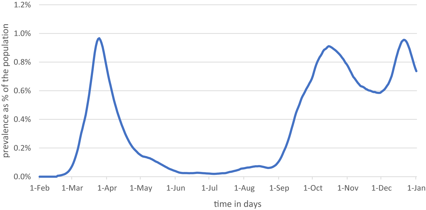
Figure 1. Estimated prevalence of COVID-19 in the Netherlands. Source RIVMFootnote 2 and own calculations.
The global economic output gap due to COVID-19 is estimated at ~6.5 % in 2020 (Rungcharoenkitkul, Reference Rungcharoenkitkul2021). Similar to most countries, the Netherlands experienced sharp declines in economic activity. Figure 2 shows weekly economic activity, based on the OECD Weekly Tracker of GDP growth (OECD, 2023). Economic activity dropped sharply in March 2020, followed by a rapid recovery. The effects of the second wave in the fall of 2020 and winter of 2020/2021 are less pronounced. The estimated total loss in economic activity in 2020 is EUR 17 bn (2.1 %).Footnote 1
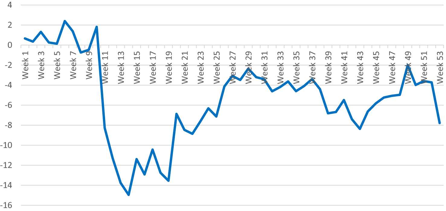
Figure 2. OECD Tracker of economic activity in 2020 (Source: OECD (2023)). Data were downloaded on 9 September 2021.
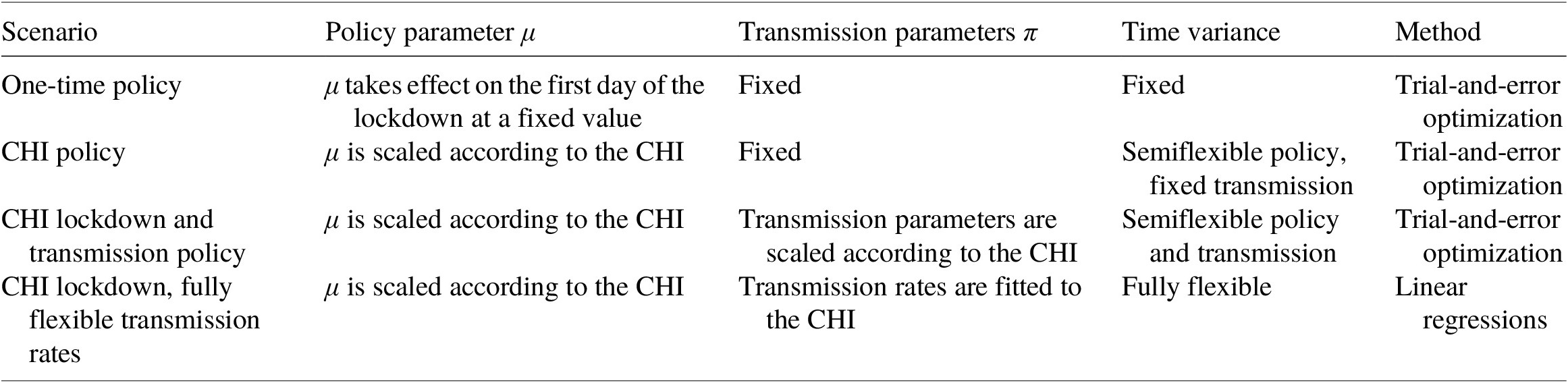
COVID-19 containment policy in the Netherlands consisted of a range of policy measures and adaptions throughout 2020. The Oxford COVID-19 Government Response Tracker of the Blavatnik School of Government weights individual containment measures into a Containment and Health Index (CHI) that reflects the stringency of COVID-19 containment policies (Hale et al., Reference Hale, Webster, Petherick, Phillips and Kira2020). Figure 3a displays the Dutch CHI. An attractive feature of the CHI is that similar indices have been composed for a wide range of countries, allowing for cross-country comparison of COVID-19 policies. For example, the CHI has been used to compare stock market volatility (Zhuo & Kumamoto, Reference Zhuo and Kumamoto2020), unemployment effects (Dreger & Gros, Reference Dreger and Gros2021), economic growth (Ashraf & Goodell, Reference Ashraf and Goodell2022), and tradeoffs between economic and health damage (Cross et al., Reference Cross, Ng and Scuffham2020; König & Winkler, Reference König and Winkler2021a).
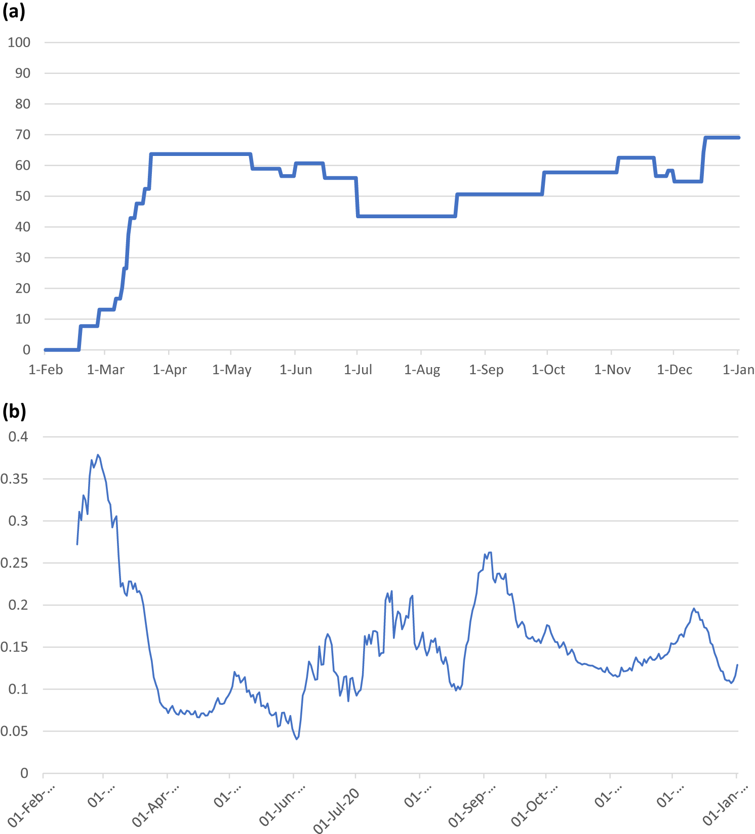
Figure 3. (a) Oxford COVID-19 Government Response Tracker of the Blavatnik School of Government Containment and Health index of the Netherlands in 2020 (Hale et al., Reference Hale, Webster, Petherick, Phillips and Kira2020). (b) Implied macro transmission rate ( $ {\rho}_t $
) in the Netherlands (Source: RIVM and own calculations).
$ {\rho}_t $
) in the Netherlands (Source: RIVM and own calculations).
3. Methods
This study adapts the Epi-econ model of Eichenbaum et al. (Reference Eichenbaum, Rebelo and Trabandt2021) to the Netherlands. The full model, including adaptations, is described in Appendix Appendix A. We pursue the following steps to assess the potential to evaluate policy options:
-
1. We parameterize the Eichenbaum, Rebelo and Trabandt (ERT) model to the Dutch pre-COVID economic and epidemiological situation (1a) and perform sensitivity analysis on the main parameters (1b).
-
2. We endeavor to reproduce observed economic and epidemiological trends by (a) a fixed-parameter calibration of policy parameters, (b) a semiflexible parameter calibration allowing policy and transmission parameters to vary over time, and (c) a fully flexible fit of the model parameters to the observed data using linear regressions
-
3. We simulate alternative policy responses by running CHI policy indices of a selection of countries through the model, as well as variants on the Dutch approach.
3.1. Step 1: Parameterization of the model
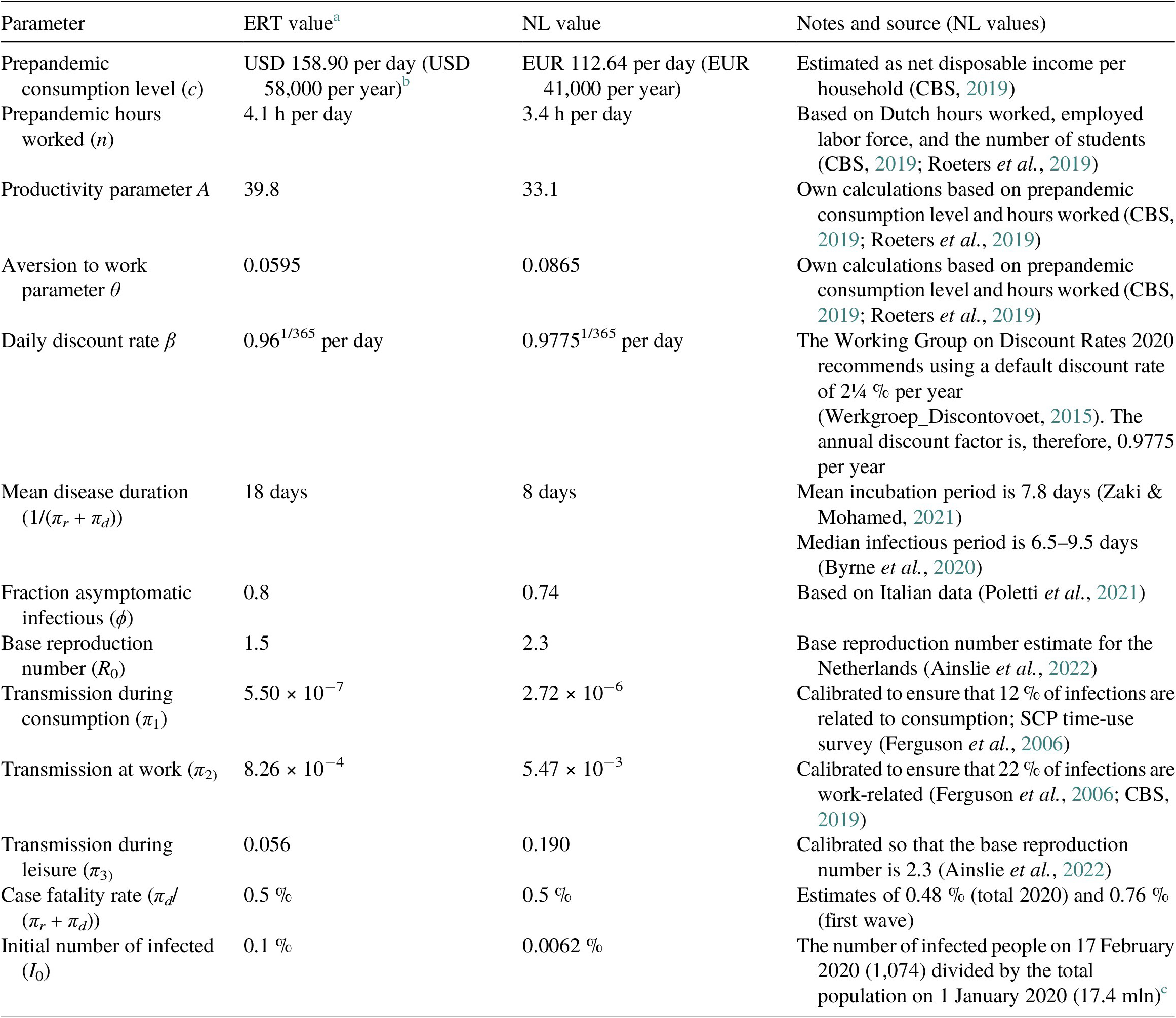
ERT uses fixed parameter values to define the initial prepandemic conditions. The modeling equations subsequently define how these parameters evolve over time during the pandemic. We adapt the main model parameter values to the Netherlands (Table 1). Country-specific discount rates, consumption levels, hours worked, and case fatality rates (CFRs) are taken from literature. To determine values for labor productivity A and the aversion-to-work parameter $ \theta $
, data on disposable income and hours worked were used.Footnote 3 We follow Eichenbaum et al. (Reference Eichenbaum, Rebelo and Trabandt2021) and Ferguson et al. (Reference Ferguson, Cummings, Fraser, Cajka, Cooley and Burke2006) who argue that in a flu epidemic, 30 % of infections occur within a household, 33 % in the overall community, and 37 % in schools and workplaces (Ferguson et al., Reference Ferguson, Cummings, Fraser, Cajka, Cooley and Burke2006; Eichenbaum et al., Reference Eichenbaum, Rebelo and Trabandt2021). We use the estimated reproduction number at the beginning of the epidemic of 2.3 (Ainslie et al., Reference Ainslie, Backer, de Boer, van Hoek, Klinkenberg, Altes, Leung, de Melker, Miura and Wallinga2022) to calculate transmission rates.Footnote 4 We utilize survey data from the Netherlands, reporting that 38 % of leisure time involves consumptive activities (Roeters et al., Reference Roeters, Bucx, Vlasblom and Voogd-Hamelink2019). As 33 % of infections occur in the general community and 38 % of time spent in the general community involves consumptive activities, it follows that 12 % (0.38 × 0.33) of infections are consumption-related.Footnote 5 An estimated 10 contacts per day in education and 4 contacts per day at work (Lee et al., Reference Lee, Brown, Cooley, Zimmerman, Wheaton, Zimmer, Grefenstette, Assi, Furphy, Wagener and Burke2010) are used to calculate infection rates at work. In the Netherlands, the working population is ~9.3 mln, while 2.6 mln people between the ages of 15 and 27 years were in education, including working students (CBS, 2019). Following Eichenbaum et al. (Reference Eichenbaum, Rebelo and Trabandt2021), 59 % of infections at work and school are attributable to work. This implies a share of infections at work of 22 % (0.59 × 0.37).Footnote 6 Next to differences in work–leisure balance, a higher base reproduction rate implies higher transmission rates for the Netherlands (e.g. 0.19 for consumption in NL vs. 0.06 in ERT). Different COVID-19 CFRs have been reported for the Netherlands, ranging from 0.76 % during the first wave and 0.48 % over 2020 (Ainslie et al., Reference Ainslie, Backer, de Boer, van Hoek, Klinkenberg, Altes, Leung, de Melker, Miura and Wallinga2022). We follow ERT in using a CFR of 0.5 %, and apply sensitivity analyses (Appendix C). Combined with a mean disease duration of 8 days (Byrne et al., Reference Byrne, McEvoy, Collins, Hunt, Casey, Barber, Butler, Griffin, Lane and McAloon2020; Zaki & Mohamed, Reference Zaki and Mohamed2021), the daily recovery rate πr becomes 0.995/8 and the daily death rate πd = 0.005/8. The sum of the recovery rate and the death rate (πr + πd) gives the percentage unsusceptible for infection (removal rate). We adjust the start number of infected persons of 0.0062 % of the population on Day 0 (17 February 2020).Footnote 7
$ \theta $
, data on disposable income and hours worked were used.Footnote 3 We follow Eichenbaum et al. (Reference Eichenbaum, Rebelo and Trabandt2021) and Ferguson et al. (Reference Ferguson, Cummings, Fraser, Cajka, Cooley and Burke2006) who argue that in a flu epidemic, 30 % of infections occur within a household, 33 % in the overall community, and 37 % in schools and workplaces (Ferguson et al., Reference Ferguson, Cummings, Fraser, Cajka, Cooley and Burke2006; Eichenbaum et al., Reference Eichenbaum, Rebelo and Trabandt2021). We use the estimated reproduction number at the beginning of the epidemic of 2.3 (Ainslie et al., Reference Ainslie, Backer, de Boer, van Hoek, Klinkenberg, Altes, Leung, de Melker, Miura and Wallinga2022) to calculate transmission rates.Footnote 4 We utilize survey data from the Netherlands, reporting that 38 % of leisure time involves consumptive activities (Roeters et al., Reference Roeters, Bucx, Vlasblom and Voogd-Hamelink2019). As 33 % of infections occur in the general community and 38 % of time spent in the general community involves consumptive activities, it follows that 12 % (0.38 × 0.33) of infections are consumption-related.Footnote 5 An estimated 10 contacts per day in education and 4 contacts per day at work (Lee et al., Reference Lee, Brown, Cooley, Zimmerman, Wheaton, Zimmer, Grefenstette, Assi, Furphy, Wagener and Burke2010) are used to calculate infection rates at work. In the Netherlands, the working population is ~9.3 mln, while 2.6 mln people between the ages of 15 and 27 years were in education, including working students (CBS, 2019). Following Eichenbaum et al. (Reference Eichenbaum, Rebelo and Trabandt2021), 59 % of infections at work and school are attributable to work. This implies a share of infections at work of 22 % (0.59 × 0.37).Footnote 6 Next to differences in work–leisure balance, a higher base reproduction rate implies higher transmission rates for the Netherlands (e.g. 0.19 for consumption in NL vs. 0.06 in ERT). Different COVID-19 CFRs have been reported for the Netherlands, ranging from 0.76 % during the first wave and 0.48 % over 2020 (Ainslie et al., Reference Ainslie, Backer, de Boer, van Hoek, Klinkenberg, Altes, Leung, de Melker, Miura and Wallinga2022). We follow ERT in using a CFR of 0.5 %, and apply sensitivity analyses (Appendix C). Combined with a mean disease duration of 8 days (Byrne et al., Reference Byrne, McEvoy, Collins, Hunt, Casey, Barber, Butler, Griffin, Lane and McAloon2020; Zaki & Mohamed, Reference Zaki and Mohamed2021), the daily recovery rate πr becomes 0.995/8 and the daily death rate πd = 0.005/8. The sum of the recovery rate and the death rate (πr + πd) gives the percentage unsusceptible for infection (removal rate). We adjust the start number of infected persons of 0.0062 % of the population on Day 0 (17 February 2020).Footnote 7
Table 1. Calibrated model parameters
a We have translated ERT calibration to a per day step.
b The average USD-EUR exchange rate during 2020 is 1.14 USD = 1 EUR (OECD). American households are on average 10-15 % larger than Dutch households (UN).
3.2. Step 2: Model fitting
The second step aims to calibrate the policy and transmission parameters to empirically observe Epi-econ trends (Di Bartolomeo et al., Reference Di Bartolomeo, D’Imperio and Felici2022). Economic lockdown parameters, modeled by μ, apply constraints on consumption and economic activity, which can be tightened or relaxed over time. Transmission rates, modeled by π, are partly determined by fixed biological traits of the virus such as infectivity – although these traits may vary between virus variants – and partly by policy measures such as social distancing and protective measures. This renders two time-variant parameters (πt and μt) that allow us to fit the model to the actual data (Anzum & Islam, Reference Anzum and Islam2021; Haw et al., Reference Haw, Morgenstern, Forchini, Johnson, Doohan, Smith and Hauck2022). In a stepwise approach, we start with fixed parameter values and relax this assumption gradually. The steps are presented in Table 2.
Table 2. Parameterization steps to improve model fit to observed trends
First, we assume transmission parameters to be invariant and the policy parameter value μ to take effect at the start of the lockdown and be retained throughout the year. Next, we allow incremental changes to μ. Using trial-and-error optimization, we scale the policy parameter to the NL-CHI. Next, additional flexibility is assumed by allowing infection transmission parameters to be affected by policy (Eichenbaum et al., Reference Eichenbaum, Rebelo and Trabandt2022). Again, we allow incremental changes over time by scaling the infection transmission rates to the CHI using trial-and-error optimization to match observed trends (Buckman et al., Reference Buckman, Glick, Lansing, Petrosky-Nadeau and Seitelman2020). Finally, we endogenize time-varying variables (Ho et al., Reference Ho, Lubik and Matthes2023).
To calibrate transmission parameters, we calculate the macro transmission rate $ {\rho}_t $
(see Appendix Appendix B for more detail). Figure 3b shows the evolution of the macro transmission rate in the Netherlands in 2020. A sharp decline during the first lockdown is followed by waves of abrupt changes and day-to-day fluctuations. The macro transmission rate is affected by a number of endogenous and exogenous factors, such as social distancing, hygiene policies, and meteorological circumstances, as well as the containment rate (Chudik et al., Reference Chudik, Pesaran and Rebucci2021). Evidently, policies aimed at restricting contacts and reducing contact transmissibility affect the macro transmission rate. The feedback loop between economic behavior and epidemiological trends may also affect the macro transmission rate variance. The variation of the macro transmission rate can be disaggregated into a part affected by policy and an unexplained part. Using linear regression models, we estimate how ρ
t is affected by policy:
$ {\rho}_t $
(see Appendix Appendix B for more detail). Figure 3b shows the evolution of the macro transmission rate in the Netherlands in 2020. A sharp decline during the first lockdown is followed by waves of abrupt changes and day-to-day fluctuations. The macro transmission rate is affected by a number of endogenous and exogenous factors, such as social distancing, hygiene policies, and meteorological circumstances, as well as the containment rate (Chudik et al., Reference Chudik, Pesaran and Rebucci2021). Evidently, policies aimed at restricting contacts and reducing contact transmissibility affect the macro transmission rate. The feedback loop between economic behavior and epidemiological trends may also affect the macro transmission rate variance. The variation of the macro transmission rate can be disaggregated into a part affected by policy and an unexplained part. Using linear regression models, we estimate how ρ
t is affected by policy:
 $$ {\rho}_t={\beta}_0+{\beta}_1{\mathrm{CHI}}_t+{\beta}_2{s}_t+\varepsilon $$
where following Ainslie et al. (Reference Ainslie, Backer, de Boer, van Hoek, Klinkenberg, Altes, Leung, de Melker, Miura and Wallinga2022), we add a seasonal variable st
Footnote 8 (Ainslie et al., Reference Ainslie, Backer, de Boer, van Hoek, Klinkenberg, Altes, Leung, de Melker, Miura and Wallinga2022). We incorporate the variation in $ {\rho}_t $
not explained by the CHI into the transmission parameters to allow daily epidemiological fluctuations in the model. We use the fitted values to estimate the effects of policy relative to endogenous effects (Appendix C). We assume that policy has a constant effect on the macro transmission rate. In reality, however, policy effects may be nonlinear, for example, larger changes in the CHI render disproportionately larger effects on the transmission parameters, on top of the existing nonlinear effects in the model. In a sensitivity analysis, we explore potential nonlinear policy effects by adding nonlinear specifications of CHI.
$ {\rho}_t $
not explained by the CHI into the transmission parameters to allow daily epidemiological fluctuations in the model. We use the fitted values to estimate the effects of policy relative to endogenous effects (Appendix C). We assume that policy has a constant effect on the macro transmission rate. In reality, however, policy effects may be nonlinear, for example, larger changes in the CHI render disproportionately larger effects on the transmission parameters, on top of the existing nonlinear effects in the model. In a sensitivity analysis, we explore potential nonlinear policy effects by adding nonlinear specifications of CHI.
3.3. Step 3: Analyzing alternative policy scenarios
Next, we estimate alternative policy responses by replacing the Dutch CHI with the CHI of a selection of countries. Representing a more lenient and a more stringent approach, respectively, we chose the Swedish and the Korean CHI (Krueger et al., Reference Krueger, Uhlig and Xie2022). As shown in Figure 4, Korea adopted a more stringent response, particularly in the first wave, while Sweden was less stringent in both waves (Bricco et al., Reference Bricco, Misch and Solovyeva2020). Korean policy would mainly simulate an earlier anticipation by the Netherlands. Interestingly, the Dutch COIVD policy was more lenient during the summer than either Sweden or Korea.
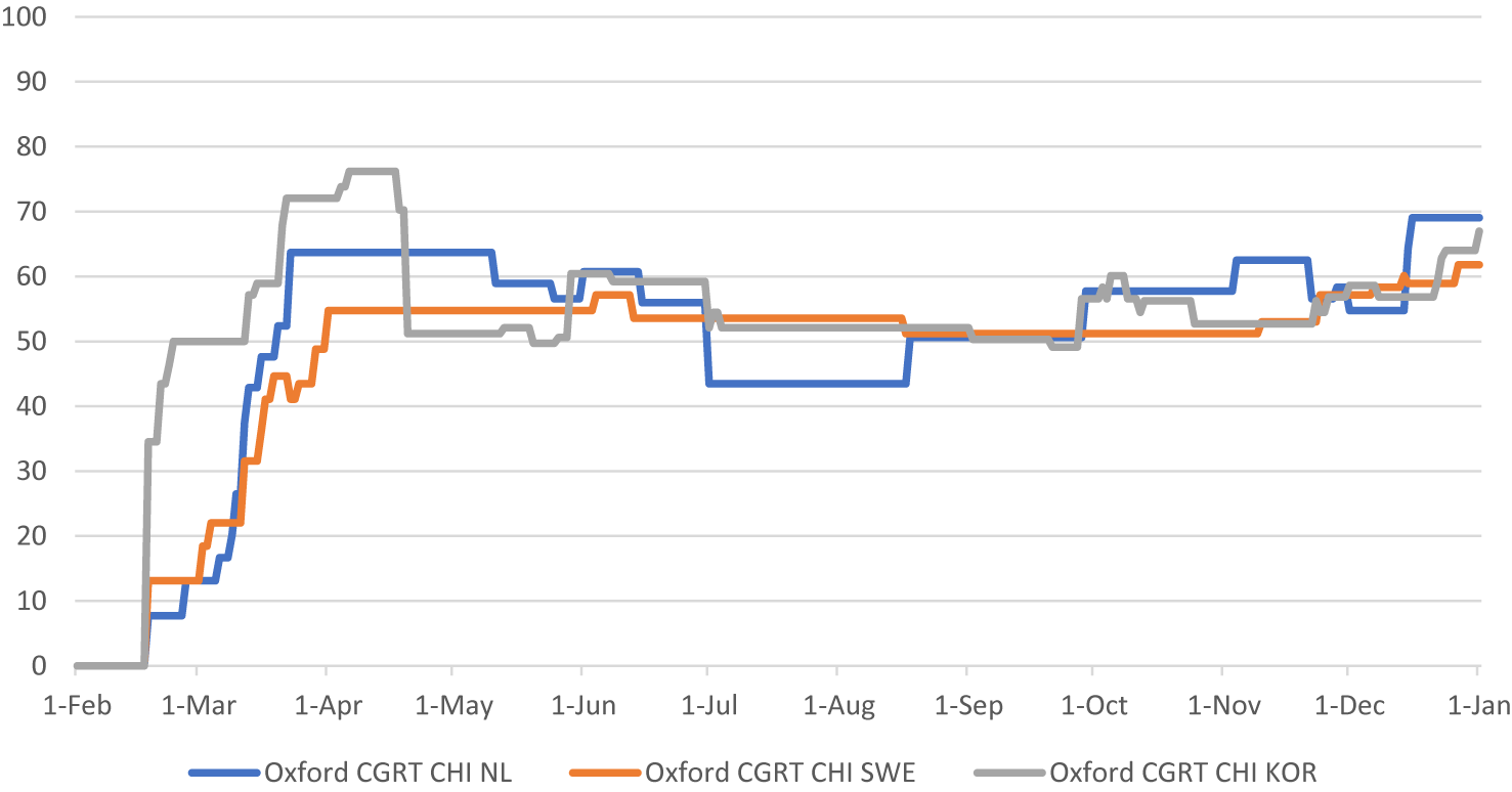
Figure 4. Containment and health index (CHI) for the Netherlands, Sweden, and Korea (Source: Blavatnik School of Government, University of Oxford).
Finally, we evaluated the effects of excluding a lockdown measure from the Dutch CHI, namely the closure of “workplaces” (Figure 5). This involves closing restaurants, shops, and so forth. It does not concern the stay-at-home or work-from-home policies. The measure of workplace closings could be interchanged readily with any other measure that renders similar effects on the overall CHI, since the CHI does not discriminate between relative effects of measures. Therefore, this could be considered as a general example of a less stringent policy.
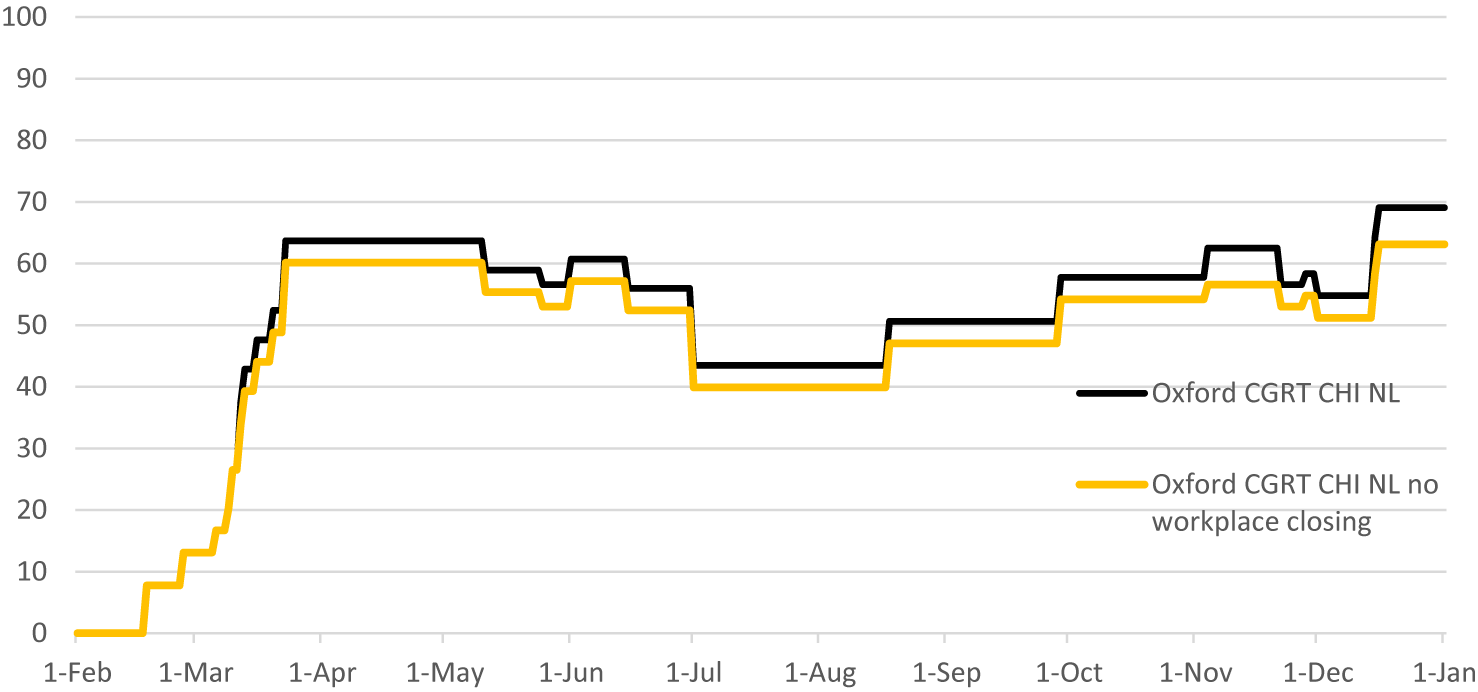
Figure 5. Containment and health index (CHI) for the Netherlands, excluding workplace closing (Source: Blavatnik School of Government, University of Oxford, and authors’ calculations).
4. Results
4.1. Step 1: Baseline simulation
Figure 6 shows the predicted Epi-econ development in the absence of policy. The simulated epidemic prevalence peaks 69 days after the initial introduction at almost 16 % of the population. This is much later than the actual epidemic (peaking after 37 days) and significantly higher than the observed trends (under 1 %). The model predicts that over 75 % of the population will become infected after the first wave, leaving no potential for a second wave. Furthermore, the baseline simulation shows an initial economic contraction of almost 35 %, which is much severe than the observed trends (15 %). The simulated contraction is followed by a rapid recovery, which is also much faster than the observed trends. One explanation is that the baseline simulation does not include COVID-19 containment policies. It is noteworthy that in the baseline simulation, after 37 days, prevalence is just over 1 % of the population.
Figure 6. Baseline simulation: (a) COVID-19 prevalence per day; (b) economic activity per day.
4.2. Sensitivity analyses
To gauge the effects of the Epi-econ feedback loop, we run the model without interaction between economy and epidemic (SIR) in comparison (Appendix C). Without the Epi-econ feedback loop, the predicted peak prevalence is 6 % points higher, but economic decline is much less severe, as any reduction in hours worked is only due to COVID-19 absenteeism and death.
Some model parameters were updated relative to the original model. A higher reproduction parameter of 2.3 (Ainslie et al., Reference Ainslie, Backer, de Boer, van Hoek, Klinkenberg, Altes, Leung, de Melker, Miura and Wallinga2022), relative to 1.5 assumed by Eichenbaum et al. (Reference Eichenbaum, Rebelo and Trabandt2021), results in a steeper and higher infection peak, with tantamount effects on the economy (Appendix C). A lower discount rate of 2.25 % per annum (Werkgroep_Discontovoet, Reference Van Ewijk, Hoen, Doorbosch, Reininga, Geurts, Visser, Bongers, van Winden, Jonker, Elsenburg, Mink, Huizinga, Aalbers, Vollebergh, Renes, Dietz, de Zeeuw, de Jong, Koopmans and Pomp2015) versus 4 % per annum intensifies the economic recession and thereby dampens the epidemic (Appendix C). As a lower discount rate places additional value on future consumption, economic activity is scaled down to reduce the risk of infection and subsequent mortality. The value of the productivity parameter for infected people (ϕI), set at 0.74 in the baseline model, shows little effect on the model outcomes (Appendix C). This is due to counterbalancing effects: while reduced productivity negatively affects hours worked of susceptibles, this effect is counteracted by a reduced risk of encountering the infected individuals while consuming. The mean infection period of 8 days was subjected to sensitivity analyses (12 days, Appendix C). While a longer infection period significantly affects the length and impact of the first wave, economic effects are smaller due to the counteracting mechanisms described above. Finally, a CFR of 1 % instead of 0.5 % reduces the peak of the first wave, but significantly increases the economic decline. Evidently, working and consuming become more costly in terms of foregone expected future utility, thereby reducing economic activity, which puts a brake on the epidemic.
4.3. Step 2: Calibrating policy parameters
Following Eichenbaum et al. (Reference Eichenbaum, Rebelo and Trabandt2021), we introduce policy through the containment rate μt. We calibrate μ to attain a peak prevalence of 1 %, in accordance with observed peak prevalence. However, even at a maximum value of μ of 100 %, peak prevalence is still much higher than observed at over 11 %, while the economic contraction is over 50 %. We conclude that a fixed policy parameter μ by itself is insufficient to simulate observed developments (Figure 7).
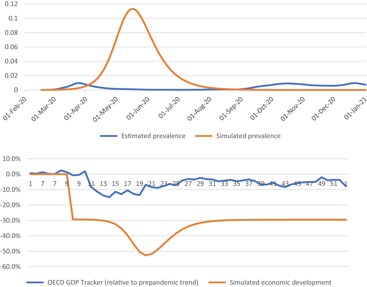
Figure 7. Simulation results for μ = 100 %.
Subsequently, we assume a semiflexible time variant and scale μt proportionally to the CHI of the Netherlands. As the observed peak prevalence is beyond reach with any μt, we calibrate μt to match the observed economic trends in the first acute phase of the epidemic, given the actual epidemic development. The subsequent recovery of the economy may be influenced by factors outside of the model, such as fiscal support packages and increasingly efficient adaptation of economic activity to COVID-19 circumstances. The first shock, however, can only be attributed to the epidemic itself and the initial policy response to it. Using a trial-and-error fitting, a calibrated value of $ {\mu}_t=0.005{\mathrm{CHI}}_t $
is obtained.
$ {\mu}_t=0.005{\mathrm{CHI}}_t $
is obtained.
Finally, we allow transmission parameters to be affected by policy. We calibrated the transmission parameters to the implied macro transmission rate ρt. This allows the model to mimic the epidemiological trends. Concurrently, we use $ {\mu}_t=0.005{\mathrm{CHI}}_t $
and add a linear trend in economic development, reflecting increasing adaptation to the circumstances (e.g. better facilities to work from home). As expected, the model closely mimics the observed epidemiological trends and produces an acceptable fit to the economic trends (Figure 8). Additional analyses reveal that this renders a policy parameter, which is relatively influential, explaining 87 % of epidemic and 70 % of economic effects relative to endogenous Epi-econ effects (Appendix C).
$ {\mu}_t=0.005{\mathrm{CHI}}_t $
and add a linear trend in economic development, reflecting increasing adaptation to the circumstances (e.g. better facilities to work from home). As expected, the model closely mimics the observed epidemiological trends and produces an acceptable fit to the economic trends (Figure 8). Additional analyses reveal that this renders a policy parameter, which is relatively influential, explaining 87 % of epidemic and 70 % of economic effects relative to endogenous Epi-econ effects (Appendix C).
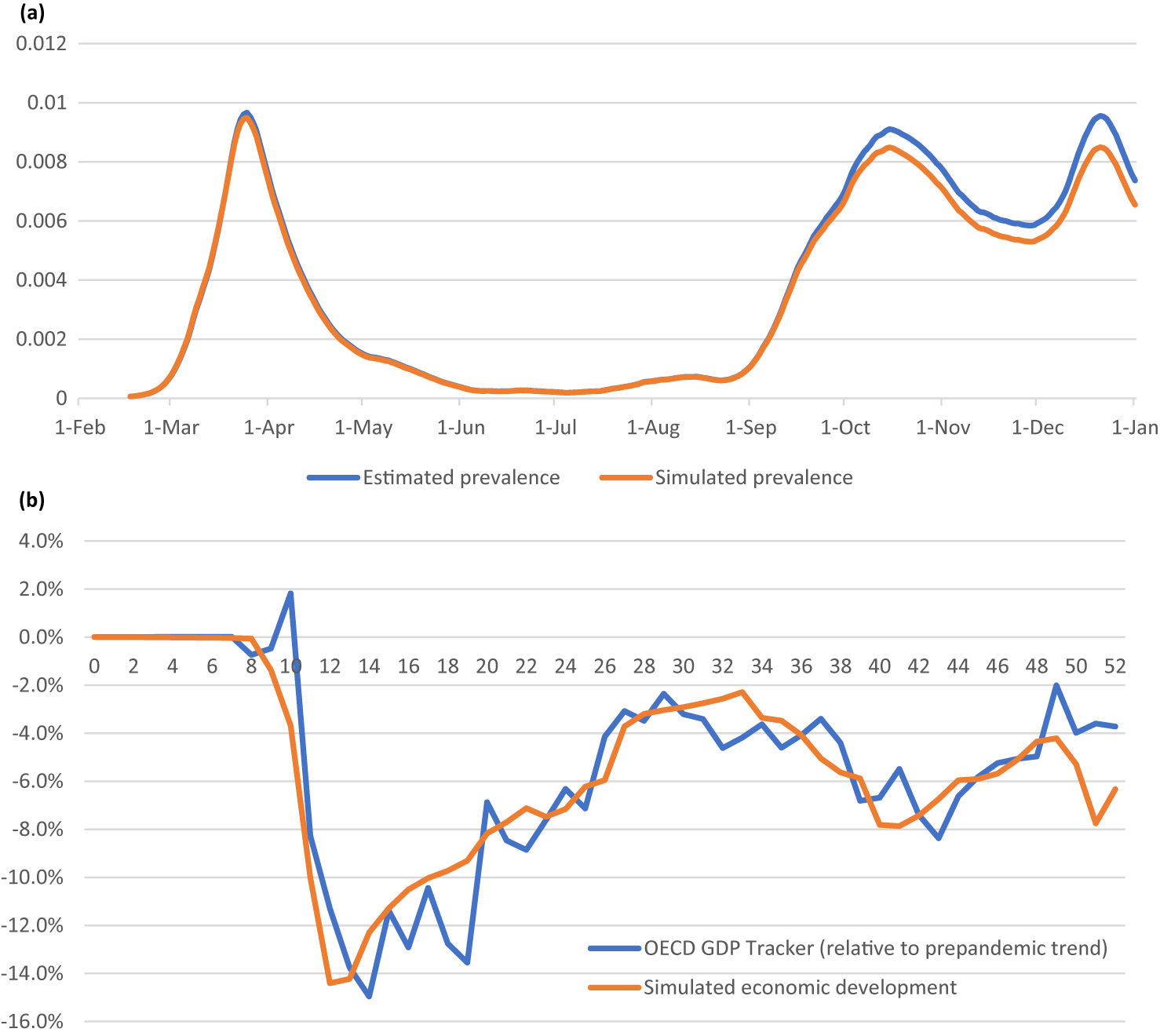
Figure 8. Actual and simulated epidemic (a) and economic development (b).
4.4. Step 3: Alternative policy simulations
We estimated the effect of policy on ρt using linear regression (Table 3). A significant effect is obtained, with an increase of one point on the CHI translating to a 0.0039 point reduction in ρt. To test the assumption that policy affects the reproduction rate in a nonlinear manner, additional linear regressions incorporating nonlinear terms and seasonal trends are estimated. The nonlinear terms are statistically significant, although with limited effects on the overall explanatory power. Marginal analysis (Appendix D) reveals that the linear term does provide a good approximation at relevant 2020 values. The seasonal trend is also significant, but its inclusion does not affect the policy coefficient. For the sake of simplicity and to avoid overfitting, we incorporate the linear term only in the model. This implies that the coefficient for CHI from the main regression model is used as a parameter to test the effect of different CHI policy evolutions.
Table 3. Estimating the effect of policy on the macro transmission rate
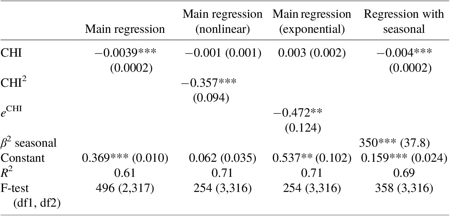
Note: Standard errors are in parentheses. Significance: *p < .05; **p < 0.01; ***p < 0.001.
Next, we substitute the NL-CHI for the CHI of Sweden and Korea, recalculate ρt and μt and rerun the model. Figure 9 shows that the application of the Swedish CHI to the Netherlands would increase (peak) prevalence, both during the first and second wave. At the end of 2020, this would have increased cumulative prevalence by 7 percentage points (51 %). However, economic trends are similar. This is because the economy faces two countervailing influences. More lenient policies directly stimulate economic activity. At the same time, more lenient policies increase infectivity and epidemic activity, which has a deterring effect on economic activity.
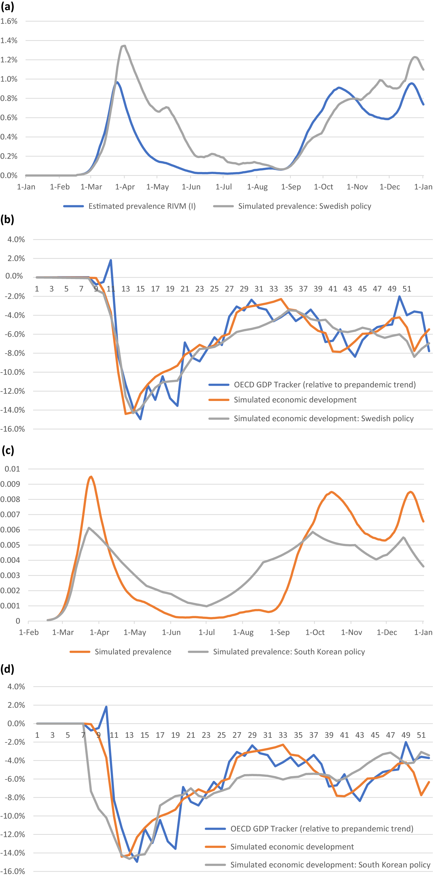
Figure 9. Model estimates for alternative CHI of Sweden (a, b) and Korea (c, d) compared to base simulations and observed trends.
Applying the Korean CHI to the Netherlands shows significant economic decline at the start of the first wave. On the other hand, peak prevalence was reduced by a third, and while prevalence would be higher during the summer, the second peak would have been lower too, with positive effects on economic activity. At the end of 2020, this strategy was estimated to result in 0.1 percentage point lower total prevalence (0.5 %) and 0.5 percentage points of additional economic decline (10 %).
Finally, we exclude a single measure (workplace closings) from the Dutch CHI as an example to simulate a more lenient lockdown policy (Figure 10). Surprisingly, the model shows limited effects during the first wave, and a very large secondary spike in COVID-19 prevalence. A large economic decline results, generated by behavioral responses to high infection rates. In the autumn of 2020, this effect would have dominated the favorable direct economic consequences of a less stringent policy. While excluding the measure (workplace closing) did reduce relative stringency slightly more during the second wave compared to the first wave, the effects are highly disproportional. This is the result of stringency during the first wave and a summer lapse. As infection rates climb, lacking the instrument of workplace closings (and putting nothing in to replace it – as we assume) shows the power of exponential growth. We also hypothesize that reduced policy adherence may be partly reflected in the unexplained part of the infectivity parameter, aggravating the effects of a less stringent policy during the second wave. This would be an interesting area for future research.
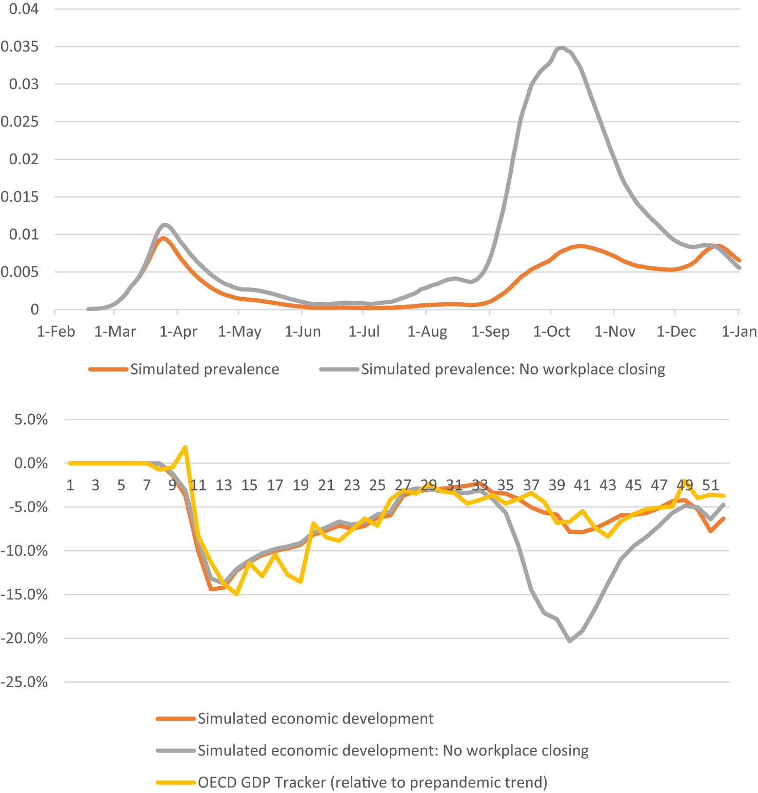
Figure 10. Model estimates for a more lenient Dutch CHI (excluding workplace closings).
Table 4 summarizes the results in terms of the number of infected persons and economic damages in 2020. The results show that the sole SIR model is poorly equipped to estimate economic losses, and tend to overestimate the incidence of infections. The ERT model (excluding policy) better captures the tradeoffs between economic and epidemiologic activity, but tends to display marginal reductions in infections at significant economic loss. Adding policy measures tends to significantly reduce economic activity at limited gains in epidemic containment. The ERT model shows a large mismatch with observed trends. Our modifications show a significant improvement in overall fit, and a more realistic tradeoff over alternative policy scenarios. A complete cost–benefit analysis would require, besides estimating the costs of infectivity, incorporating additional policy effects (e.g. regular care delays, mental health effects of lockdowns and economic decline, etc.).
Table 4. Summary of model outcomes

5. Conclusion and discussion
To explore the feasibility of Epi-econ models for evaluating alternative policy measures, we adopted the seminal Epi-econ model of Eichenbaum et al. (Reference Eichenbaum, Rebelo and Trabandt2021) to simulate the Dutch Epi-econ trends. We applied the Dutch parameters and updated existing parameters to the latest scientific insights. We found that the model performed poorly in simulating observed trends, and degrees of freedom in the model policy parameters were too small to generate realistic model outcomes. Subsequently, we systematically increased the flexibility of the model to improve fit, by first adding time flexibility to the policy parameters and, next, by adding time-variant policy influence on transmission parameters. This allowed for coupling the CHI to the model and incorporating policy responses related to voluntary mitigating behavior other than reductions in work and consumption. To further improve the model fit, linear regression estimation was used to isolate the effects of policy on transmission parameters. These rigorous alterations of the model did allow testing alternative policy scenarios in a realistic model setting with reasonable face validity. We found that a more stringent lockdown policy (e.g. as enacted by the Republic of Korea) would reduce peak prevalence and aggravate peak economic contraction, with little effect on overall trends. Conversely, more lenient lockdown policies (e.g. as enacted by Sweden) were estimated to increase peak and overall prevalence, with little effect on economic outcomes. This is due to two opposing forces: first, more lenient policies result in more economic activity. However, increased chances to become infected discourage economic activity. Too lenient measures, therefore, could rapidly increase overall infections and thereby harm the economy even more than stricter measures. The model allows qualitative appraisal of alternative policy scenarios and highlights complicated interrelations between economic and epidemiological trends. However, model validity declines for more impactful policy alternatives (e.g. workplace closings), as the nonlinear nature of the model makes it sensitive to underlying assumptions and parameter values, such as policy adherence.
These results are in line with other literature, finding a weak tradeoff between economic damage and infection rates and preferring stronger lockdowns (Flaschel et al., Reference Flaschel, Galanis, Tavani and Veneziani2021; Gallic et al., Reference Gallic, Lubrano and Michel2022). Using a simple SIR model and a double sigmoid fitting methodology, Gallic et al. (Reference Gallic, Lubrano and Michel2022) argue that the Netherlands and Sweden would have been better off employing a stricter lockdown policy such as that of Denmark’s (Gallic et al., Reference Gallic, Lubrano and Michel2022). Born et al. (Reference Born, Dietrich and Müller2021) construct a counterfactual lockdown policy for Sweden, and find that a stricter lockdown would have reduced the number of deaths without significant effects on economic output. Alfano et al. (Reference Alfano, Ercolano and Pinto2022) find that the nonlinear effect on economic decline may be due to the limited capability of fiscal policy to counteract negative lockdown effects. Bognanni et al (Reference Bognanni, Hanley, Kolliner and Mitman2020) find that mitigation measures can have positive effects on both transmission and economic damage. Hsu et al. (Reference Hsu, Lin and Yang2020) estimate real income losses of 30–37 % due to suboptimal policy in the context of the United States. Borelli and Góes (Reference Borelli and Góes2021) apply the ERT model to the COVID-19 policy in Brazil, and found substantial divergence to the actual trends, relating to the initial percentage of infections, and the exclusion of modeling new strains. Applying DSGE economic modeling to OECD data, Cardani et al. (Reference Cardani, Croitorov, Giovannini, Pfeiffer, Ratto and Vogel2021) find that lockdown effects are a predominant factor in explaining economic contraction. However, the authors do not distinguish between forced and voluntary lockdown behavior (Cardani et al., Reference Cardani, Croitorov, Giovannini, Pfeiffer, Ratto and Vogel2021). Other authors also argue that no tradeoff between health and economic damage need to exist; for example, under specific conditions, quarantines can reduce both infections and economic damage (Goenka et al., Reference Goenka, Liu and Nguyen2020). Strict social policy measures and targeted isolation may reduce both infections and damage due to shorter lockdown periods (Kahalé, Reference Kahalé2020; Ash et al., Reference Ash, Bento, Kaffine, Rao and Bento2022).
However, a number of limitations apply. First, the model of Eichenbaum et al. (Reference Eichenbaum, Rebelo and Trabandt2021) employs a relative straightforward approach to model Epi-econ effects. For example, the SIR model employed by ERT does not account for the possibility of reinfection, international travel or viral mutations. More elaborate models are available to assess the epidemiological effects of policy measures for the Netherlands in isolation (e.g. see Ainslie et al., Reference Ainslie, Backer, de Boer, van Hoek, Klinkenberg, Altes, Leung, de Melker, Miura and Wallinga2022). However, it is an open question whether more advanced models have better predictive performance (Roda et al., Reference Roda, Varughese, Han and Li2020). Furthermore, policy recommendations may require information on multiple interrelated outcome measures, necessitating more simplistic cross-over models. Policy recommendations also could benefit from multiple models to reduce potential idiosyncratic modeling errors (Ahn et al., Reference Ahn, Silberholz, Song and Wu2021). Ideally, the integration of specialized and generic models allows adequate incorporation of all relevant policy effects. Second, our model abstracts from fiscal policy or vaccination policies. Additional fiscal policy can reduce economic damage (Di Bartolomeo et al., Reference Di Bartolomeo, D’Imperio and Felici2022). For example, many governments provided fiscal support to those affected by lockdown policies, to dampen long-term economic decline (Gatti & Reissl, Reference Delli Gatti and Reissl2020). Governments may respond to Epi-econ trends through supplementary fiscal support policies, adding a layer of complexity to the model (Siddik, Reference Siddik2020). The propensity of governments to provide fiscal support is likely to affect behavior, and thereby the economic and epidemiological effects of the lockdown policy. The same holds for expectations of vaccination availability and policy (Eichenbaum et al., Reference Eichenbaum, Rebelo and Trabandt2021; Fu et al., Reference Fu, Jin, Xiang and Wang2022; Garriga et al., Reference Garriga, Manuelli and Sanghi2022; Glover et al., Reference Glover, Heathcote and Krueger2022; Iverson et al., Reference Iverson, Karp and Peri2022). Third, additional information may be required to fully assess all costs and benefits of alternative policy measures. Outcomes, such as health effects due to delays in regular care, mental effects of lockdown policies, effects on education, investments, and long-term productivity, may differ between policy options and affect optimal policy (Dudine et al., Reference Dudine, Hellwig and Jahan2020; Oosterhoff et al., Reference Oosterhoff, Kouwenberg, Rotteveel, Van Vliet, Stadhouders, De Wit and Van Giessen2023). Furthermore, the effects of biological changes to the severe acute respiratory syndrome coronavirus 2 virus over time (e.g. infectivity of different strains) are not taken into account. Fourth, behavioral responses are likely to be complex, being time-, context-, and path-dependent. For example, behavioral responses to mitigate infection risk may increase when the health system becomes crowded and accessibility is reduced (Hamano et al., Reference Hamano, Katayama and Kubota2020). Moreover, policy compliance is likely to decrease over time. We find some evidence in our results on workplace closings that similar policy changes have highly divergent effects in different waves. Incorporating assumptions regarding declining attention to the epidemic over time was shown improve the model fit (Diez de los Rios, Reference Diez de los Rios2022). If future expectations are correlated to current policy measures, model outcomes may be biased. For example, a swift and strict policy response to the first wave may set a precedent for next waves and influence public expectations. Therefore, a strategy of temporal policy changes may increase effectiveness (Pataro et al., Reference Pataro, Oliveira, Morato, Amad, Ramos, Pereira, Silva, Jorge, Andrade and Barreto2021). We find that policy is relatively influential, contrary to some evidence suggesting the dominance of endogenous responses (Goolsbee & Syverson, Reference Goolsbee and Syverson2021; Herby, Reference Herby2021). Combined with the overestimations of the Epi-econ model, this could indicate an incomplete or insufficiently strong Epi-econ feedback loop. Additional research is required to distinguish between endogenous responses and policy responses (Hamilton et al., Reference Hamilton, Haghpanah, Tulchinsky, Kipshidze, Poleon, Lin, Du, Gardner and Klein2024). Fifth, we used the CHI to model the lockdown policy under the assumption that equal changes in the CHI reflect equal-sized policy effects. The CHI is not necessarily constructed to fulfill this assumption, reducing the precision of the policy variable. However, to scale the CHI to reflect the relative size of the effect of each individual constituent policy is beyond the scope of this article. Furthermore, the effects of changes in the CHI may be nonlinear, irrespective of the underlying measures. We find evidence that larger changes in the CHI have a disproportionately larger effect. This implies that our linear approximation is mainly valid for small changes in the CHI, and for larger changes, more elaborate modeling is required. We also find that policy changes may have nonlinear effects on infectivity, although the effects at the margin seem limited. Possibly, the adjustment from weekly time steps to daily time steps in the model, combined with growth rates being modeled exponentially, could cause linear approximations to resemble nonlinear policy effects. Moreover, we assume that policy affects epidemic trends within the same time step, while the actual causal mechanism may cross multiple time steps and may include reverse causality. This is true for Epi-econ models in general. Finding the appropriate causal and temporal structure to incorporate policy measures in modeling is a promising area for future research. Last, we use the CHI of two countries as proxies for more lenient and more strict policies, while acknowledging that the CHI is a result of country-specific cultural, political, and behavioral factors. Any CHI applied to a different country is likely to produce different results. In this light, the alternative policy paths should be viewed as crude approximations that do not reflect any resemblance with the specific countries. Furthermore, it is not guaranteed that the alternative policy paths were compliant with the actual policy space of the Netherlands.
A number of potential lines of research could improve the applicability of Epi-econ models for policy evaluation. For example, the model does not stratify between important population groups, such as age groups or sectors, nor do they extent Epi-models with confounding factors such as international mobility, seasonal effects or path dependency. Differentiating between age, disease state, region, work status, employment and consumption sector, gender, or income groups could improve model validity (Campos et al., Reference Campos, Cysne, Madureira and Mendes2021; Mahmoudi, Reference Mahmoudi2022; Giagheddu & Papetti, Reference Giagheddu and Papetti2023). Makris (Reference Makris2021) estimated an SIR model with multiple population groups and sectors. Other authors only use multiple age cohorts (Acemoglu et al., Reference Acemoglu, Chernozhukov, Werning and Whinston2020; Glover et al., Reference Glover, Heathcote, Krueger and Ríos-Rull2020; Jaouimaa et al., Reference Jaouimaa, Dempsey, Van Osch, Kinsella, Burke, Wyse and Sweeney2021; La Torre et al., Reference La Torre, Liuzzi, Maggistro and Marsiglio2022). Identifying unique groups with differing mechanisms relating infection and transmission to economic effects could improve model performance, but identifying these causal mechanisms is likely to be complicated. By incorporating “random noise,” our modeling approach implicitly takes into account factors such as voluntary social-distancing behavior, as well as policy compliance, productivity at home, environmental influences, and other factors that can drive temporal variation in infectivity. However, these interactions remain implicit, and future modeling could benefit from explicit causal incorporation of these behavioral effects and policy interactions. Other potential additions include spatial modeling (Bisin & Moro, Reference Bisin and Moro2020, Reference Bisin and Moro2022; Bognanni et al., Reference Bognanni, Hanley, Kolliner and Mitman2020), uncertainty surrounding infectivity (Forsyth, Reference Forsyth2020), and social learning (Davids et al., Reference Davids, Du Rand, Georg, Koziol and Schasfoort2023). While the model employed here has discrete time steps of a day, more elaborate infectious disease models are often specified in continuous time. Wacker and Schlüter (Reference Wacker and Schlüter2020) show that a discrete-time SIR model has the same properties as a continuous-time SIR model, and that key variables (e.g. the R-number) also have a comparable interpretation (Wacker & Schlüter, Reference Wacker and Schlüter2020). Furthermore, any difference is always bounded, and decreases as the time steps of the discrete time SIR model are shorter. Alternatively, a fully empirical approach could be pursued, for example, to assume independence between Epi-econ trends and separately estimate the effects of policy measures. However, the complex, adaptive nature of both trends would likely reduce the validity of the outcomes when analyzed separately. In all cases, a common denominator needs to be constructed to compare health effects and economic effects. While COVID-19 infections could be converted to quality-adjusted life years, the incorporation of more general health effects requires additional efforts.
Despite the shortcomings, the adjusted Epi-econ model does produce policy-relevant insights. Different lockdown policy approaches would have significantly affected the epidemiological trends. More strict policies could have reduced peak prevalence, especially during the first wave. Here, timing is important to reduce both economic damage and health damage (Cross et al., Reference Cross, Ng and Scuffham2020). Pursuing a policy approach similar to that of Korea’s in the Netherlands could have resulted in a more evenly distributed number of infections. Given the high strain on the Dutch healthcare system, especially during the first wave, this could have been a promising policy strategy. Especially as the model shows a weak tradeoff between epidemiology and economic development in this scenario, the expected economic decline is similar to the baseline scenario. Conversely, a less stringent policy approach similar to the Swedish strategy would have increased infection prevalence without a major effect on economic trends. Here, keeping the economy working is counterbalanced by increased disease prevalence and, as a result, endogenous reductions in economic activity. Given the large strain on the healthcare sector in the baseline scenario, a less stringent lockdown policy would have been likely undesirable, especially as the effects on the economy would have been minimal.
Differences between country lockdown policy responses were limited. When larger lockdown policy changes were assumed, for example, the removal of workplace closings from the Dutch CHI, large (negative) effects were obtained, showing nonlinear effects and high model sensitivity. However, the set of realistically attainable policy options may have been limited as well. Realistically attainable policy strategies may even be country-specific, suggesting that strategies employed by some countries may not have been a realistic option for other countries. Furthermore, uncertainty at the moment of decision-making should be taken into account (Barnett et al., Reference Barnett, Buchak and Yannelis2023). More research is needed to select policy options that are realistic and relevant alternatives for observed policies in a given country. The model is calibrated on the Netherlands, being a small, open economy. In theory, the model is generalizable to all countries that have sufficient data to calibrate the model. However, once calibrated, the model produces results unique to the specific country; different countries likely differ significantly in terms of epidemiological trends and policy effects.
To conclude, while Epi-econ models generate relevant insights into the interaction between Epi-econ trends, the models are ill-suited to quantitatively evaluate alternative policy options. We propose a number of fitting steps to improve the usability of Epi-econ models for this purpose, and show that the model can produce improved qualitative predictions of alternative policy effects. This could have significant benefits in policy evaluation: the adjusted model produced a more accurate estimate of economic damages and number of infected and a more realistic tradeoff between the two main outcomes. Additional steps are required to produce a valid quantitative prediction. Specifically, the challenge is to incorporate complex behavioral effects into relatively simple models. Furthermore, useful policy evaluation requires additional outcomes besides Epi-econ trends, such as the general health effects of the lockdown policy. The adjusted model could serve as a bridge model to connect more complex models that focus on a specific outcome (e.g. number of infected or economic activity). This could render a set of models that would enable a full assessment of costs and benefits of the lockdown policy. Nevertheless, using relatively simple adjustments to existing Epi-econ models, we show that the Netherlands could have benefited from slightly more stringent policy measures, especially during the first wave.
Funding
This work was supported by the Dutch Ministry of Health, Welfare and Sports.
A. Appendix A: Epi-econ model description
A.1. Epidemiological SIR model
The epidemiological SIR model describes how an epidemic spreads through a population (Weiss, Reference Weiss2013). It has four epidemiological stages: susceptible, infected, recovered, and deceased. Initially, the full population is susceptible, and then a small number of individuals become infected and start infecting others at reproduction rate R. Infected people either recover from their infection and enter the “recovered” category, or they die and enter the deceased category. A simplifying assumption is made that recovered people are unable to become infected again. The model of Eichenbaum et al. (Reference Eichenbaum, Rebelo and Trabandt2021) employed a time step of 1 week. To simulate the epidemic adequately, we use a time step of 1 day. The epidemiological SIR model can be described by the following equations:
 $$ \hskip-5em {S}_{t+1}={S}_t-{T}_t\hskip15em (\mathrm{susceptibles}) $$
 $$ {I}_{t+1}={I}_t+{T}_t-{\pi}_r{I}_t-{\pi}_d{I}_t\hskip7em (\mathrm{infected};\ \mathrm{prevalence}) $$
 $$ \hskip-7.3em {R}_{t+1}={R}_t+{\pi}_r{I}_t\hskip14em (\mathrm{recovered}) $$
 $$ \hskip-8em {D}_{t+1}={D}_t+{\pi}_d{I}_t\hskip13em (\mathrm{deceased}) $$
 $$ \hskip4em {T}_t={\rho}_t{S}_t{I}_t\hskip16em (\mathrm{newly}\ \mathrm{infected};\ \mathrm{incidence}) $$
 $$ \hskip-3em {\rho}_t={\pi}_1{c}_t^S{c}_t^I+{\pi}_2{n}_t^S{n}_t^I+{\pi}_3\hskip8em (\mathrm{transmission}\ \mathrm{rate}) $$
Equation (A.1) states that the number of susceptible people (St) decreases by the number of new infections (Tt). In Equation (A.2), the number of newly infected people (It + 1) is equal to the number of people infected in period t (It) plus the new infections (Tt), minus the recovered and deceased people. Infected people recover with a probability πr per day or die with a probability πd per day. This affects the number of people recovered (Rt; Equation (A.3)) and those who died (Dt; Equation (A.4)). The number of new infections (Tt) depends on the number of susceptible and infected people, mediated by the transmission rate (ρt) (Equation (A.5)). The model does not distinguish between different age groups, but it does distinguish three “settings” where infections occur, namely infections through consumption, through work and all other situations. The transmission rate depends on the chance of becoming infected during consumption ( $ {\pi}_1 $
), at work (
$ {\pi}_1 $
), at work ( $ {\pi}_2 $
) or elsewhere (
$ {\pi}_2 $
) or elsewhere ( $ {\pi}_3 $
). Equation (A.6) represents the average transmission rate (ρt) over the entire population (“macro transmission rate”). Through explicitly modeling the infection risk at work and during consumption, the Epi-model interacts with the economy: the more time people spend consuming or working, the faster the epidemic spreads through the population.
$ {\pi}_3 $
). Equation (A.6) represents the average transmission rate (ρt) over the entire population (“macro transmission rate”). Through explicitly modeling the infection risk at work and during consumption, the Epi-model interacts with the economy: the more time people spend consuming or working, the faster the epidemic spreads through the population.
For further analysis, it is useful to define two additional quantities:
 $$ {\tau}_t={T}_t/{S}_t={\pi}_1\left[\left({c}_t^S\right)\left({c}_t^I{I}_t\right)\right]+{\pi}_2\left[\left({n}_t^S\right)\left({n}_t^I{I}_t\right)\right]+{\pi}_3{I}_t $$
 $$ {R}_t^e=\frac{\rho_t{S}_t}{\pi_r+{\pi}_d} $$ $ {\tau}_t $
is the so-called force of infection. It represents the risk of infection of a susceptible person. Re is the reproduction number of the Epi-econ model.
$ {\tau}_t $
is the so-called force of infection. It represents the risk of infection of a susceptible person. Re is the reproduction number of the Epi-econ model.
A.2. Economic choice model
In the economic choice model, a representative consumer chooses work hours and consumption based on a representative utility function:
 $$ {u}_t^j=u\left({c}_t^j,{n}_t^j\right)=\ln {c}_t^j-\frac{1}{2}\theta {\left({n}_t^j\right)}^2 $$
The representative consumer faces a budget constraint that implies that to consume ( $ {c}_t^j $
), income earned by working
$ {c}_t^j $
), income earned by working $ {n}_t^j $
hours is required. Spending is restricted by a budget restriction:
$ {n}_t^j $
hours is required. Spending is restricted by a budget restriction:
 $$ {c}_t^j=\frac{A{n}_t^j{\phi}^j+{\Gamma}_t}{\left(1+{\mu}_t\right)} $$
Here, A reflects someone’s productivity, that is, wage. A simple representative business sector produces Ct consumer goods and services according to the production technology Ct = ANt, with Nt the labor demand by companies. The representative company maximizes its profit ANt – wtNt. From this follows wt = A. The factor $ {\phi}^j $
reflects productivity loss due to COVID-19 infections, where
$ {\phi}^j $
reflects productivity loss due to COVID-19 infections, where $ {\phi}^S={\phi}^R=1 $
en
$ {\phi}^S={\phi}^R=1 $
en $ 0<{\phi}^I<1 $
. In addition, everyone receives a lump-sum benefit Γt. Disposable income (
$ 0<{\phi}^I<1 $
. In addition, everyone receives a lump-sum benefit Γt. Disposable income ( $ A{\phi}^j{n}_t^j+{\Gamma}_t $
) is taxed at the rate μt. By channeling the proceeds of the lump-sum tax back to consumers, the combination of μt and Γt acts as an approximation for the restrictive measures in the economy that the government is taking to slow down the spread of COVID-19.Footnote 9 This means that the government also has a budget restriction:
$ A{\phi}^j{n}_t^j+{\Gamma}_t $
) is taxed at the rate μt. By channeling the proceeds of the lump-sum tax back to consumers, the combination of μt and Γt acts as an approximation for the restrictive measures in the economy that the government is taking to slow down the spread of COVID-19.Footnote 9 This means that the government also has a budget restriction: $ {\mu}_t\left({S}_t{c}_t^S+{I}_t{c}_t^I+{R}_t{c}_t^R\right)={\Gamma}_t\left({S}_t+{I}_t+{R}_t\right) $
. Finally, there is equilibrium in the labor market and in the market for goods and services.
$ {\mu}_t\left({S}_t{c}_t^S+{I}_t{c}_t^I+{R}_t{c}_t^R\right)={\Gamma}_t\left({S}_t+{I}_t+{R}_t\right) $
. Finally, there is equilibrium in the labor market and in the market for goods and services.
People maximize their expected lifetime utility by choosing an optimal level of work and consumption in each period t. The expected lifetime utility of a susceptible person is given as:
 $$ {U}_t^S={u}_t^S+\beta \left[\left(1-{\tau}_t\right){U}_{t+1}^S+{\tau}_t{U}_{t+1}^I\right] $$
with β as the discount factor. Equation (A.11) states that the expected lifetime utility of a susceptible person is equal to the utility of a susceptible person in the current period ( $ {u}_t^S $
), plus the expected lifetime utility from period t + 1 discounted to the current period t. With probability
$ {u}_t^S $
), plus the expected lifetime utility from period t + 1 discounted to the current period t. With probability $ {\tau}_t $
(see Equation (A.7)), a susceptible person will become infected. Becoming infected may reduce productivity during the period that a person is ill, and thus reduce consumption opportunities. Moreover, becoming infected may lead to death, which also reduces future consumption opportunities.
$ {\tau}_t $
(see Equation (A.7)), a susceptible person will become infected. Becoming infected may reduce productivity during the period that a person is ill, and thus reduce consumption opportunities. Moreover, becoming infected may lead to death, which also reduces future consumption opportunities.
The expected lifetime utility of an infected person is given as follows:
 $$ {U}_t^I={u}_t^I+\beta \left[\left(1-{\pi}_r-{\pi}_d\right){U}_{t+1}^I+{\pi}_r{U}_{t+1}^R+{\pi}_d\bullet 0\right] $$
An infected person dies from COVID-19 with probability $ {\pi}_d $
and the expected lifetime utility of a deceased person is zero. In addition, with probability
$ {\pi}_d $
and the expected lifetime utility of a deceased person is zero. In addition, with probability $ {\pi}_r $
, the infected person will recover. The probability that an infected person remains infected is
$ {\pi}_r $
, the infected person will recover. The probability that an infected person remains infected is $ \left(1-{\pi}_r-{\pi}_d\right) $
. The economic behavior of an infected person in the current period does not affect his future epidemiological status. Choices with regard to consumption and work of an infected person, therefore, only affect utility in the current period
$ \left(1-{\pi}_r-{\pi}_d\right) $
. The economic behavior of an infected person in the current period does not affect his future epidemiological status. Choices with regard to consumption and work of an infected person, therefore, only affect utility in the current period $ {u}_t^I $
.
$ {u}_t^I $
.
Similarly, the current choices of recovered persons do not affect his future epidemiological status. The expected lifetime utility of a recovered person is given as follows:
 $$ {U}_t^R={u}_t^R+\beta {U}_{t+1}^R $$
Because the representative consumer values future utility, susceptible individuals take into account that their economic activities (consuming and working) are associated with an increased likelihood of infection. Thus, even without policy intervention, it is expected that economic activity will decline when the infection rate increases. This also has consequences for the course of the epidemic. The drop in consumption and hours worked of susceptibles also leads to a drop in the macro transmission rate, and thus to a drop in the number of new infections Tt. These two mechanisms form the interaction between epidemiology and economics.
COVID-19 policy is incorporated into the model along two channels. First, preventative policies such as social distancing, washing hands, wearing face masks, and limiting group sizes lower the transmission parameters ( $ {\pi}_1,{\pi}_2,{\pi}_3 $
). Second, lockdown policies, such as closing parts of the economy, are modeled as an explicit tax on consumption (
$ {\pi}_1,{\pi}_2,{\pi}_3 $
). Second, lockdown policies, such as closing parts of the economy, are modeled as an explicit tax on consumption ( $ {\mu}_t $
). This tax reduces the attractiveness of consuming, inhibits the level of economic activity, reduces the number of contacts in consumption and work, and thus slows down the epidemic.
$ {\mu}_t $
). This tax reduces the attractiveness of consuming, inhibits the level of economic activity, reduces the number of contacts in consumption and work, and thus slows down the epidemic.
B. Appendix B: Calculating the implied macro transmission rate
By combining prevalence with the SIR part of the Epi-econ model (Equations (A.1)–(A.8) of Appendix A), we can reverse calculate the macro transmission rate ρ. Next, rewriting Equation (A.2) as:
 $$ {T}_t={I}_{t+1}-{I}_t+{\pi}_r{I}_t+{\pi}_d{I}_t $$
The first two terms at the right-hand side of Equation (B.1) are the prevalence on Day t + 1 and the prevalence on Day t. We solve for the number of people recovering from infection on Day t using the calibrated value of πr (0.124, see Table 1). As the number of recovered people (R) is zero at the start of the pandemic, the trend in the number of recovered people (Rt) in 2020 can be reverse calculated. Analogously, for the number of deaths, we use πr = 6.25 × 10E – 4.Footnote 10
As a robustness check, we compare the implied recovery rate to the estimated seroprevalence from the different rounds of the Pienter Corona survey and end-of-the-year estimates from the RIVM (Figure B1). These external measurements are in accordance with the implied recovery rate from our model.
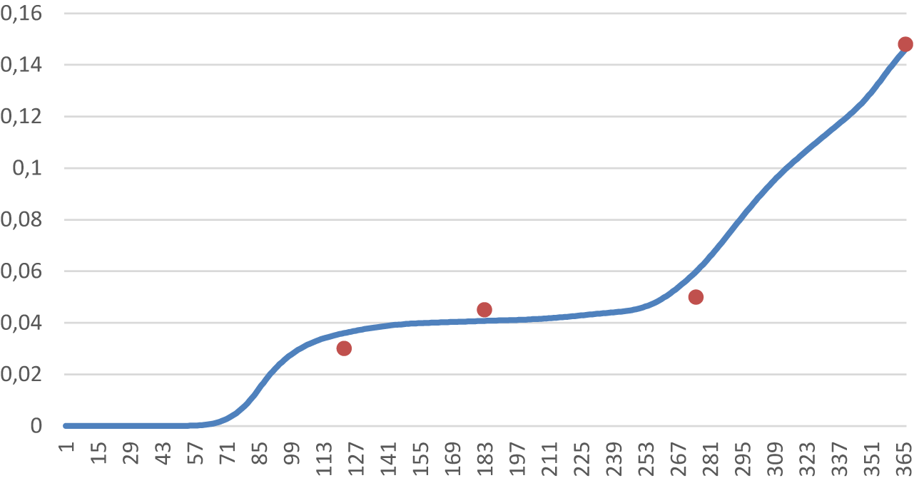
Figure B1. The number of recovered persons (Rt) modeled (blue line) compared to official measurements (red). The x-axis shows the days of 2020.
Next, we calculate the implied number of new infections (Tt, incidence), the population share of susceptible people (St), and the evolution of ρt in 2020. If we run the Epi-econ model with π 1 = π 2 = 0 (i.e. no interaction between the economy and the epidemic) with the observed macro transmission rate as input for π3, then the model exactly simulates the observed prevalence and the simulated transmission rate is also equal to the observed macro transmission rate. After all, this is how the macro transmission rate is calculated.
C. Appendix C: sensitivity analyses
Figure C1 shows the results when π 1 = π 2 = 0, implying no feedback loop between epidemiology and the economy. The value of π 3 was adjusted to compensate for the omission of other transmission channels. As expected, prevalence is higher and economic decline lower, implying that the economy reduces infectivity through voluntary action at the cost of economic activity.

Figure C1. The influence of interaction between epidemic and economy on economic and epidemiological development (the horizontal axis is the number of days since the start of the pandemic).
Next, we examine how the outcomes of the model change if we choose a lower value for the transmission rate (ρ), a lower value for the discount factor (β), a higher value for the productivity loss of infected (ϕI), a lower value for the removal rate (πr + πd), and a higher value for the CFR (πd/(πr + πd)).
C.1. Transmission rate
Using the base reproduction rate of 1.5 of Eichenbaum et al. (Reference Eichenbaum, Rebelo and Trabandt2021) implies a transmission rate ρ of 0.1875. Using the best estimate of 2.3 for the Netherlands, a transmission rate of 0.2875 is obtained. A lower transmission rate reduces peak prevalence and economic damage (Figure C2a).
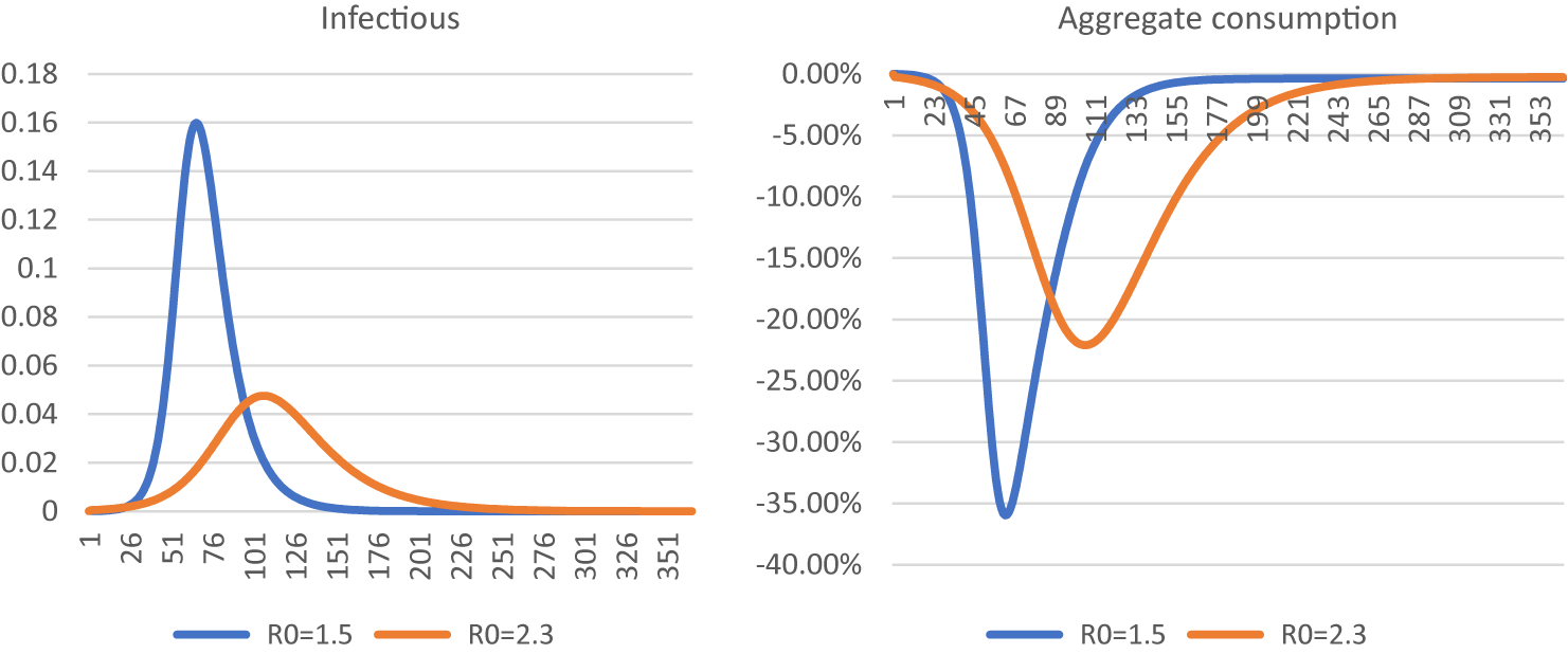
Figure C2. Simulation of the number of infectious persons (a) and aggregate consumption (b) using a base reproduction rate of 1.5 compared to the baseline model. The horizontal axis is the number of days since the start of the pandemic.
C.2. Discount rate
Using the original discount rate of 4 % from Eichenbaum et al. (Reference Eichenbaum, Rebelo and Trabandt2021) results in a less deep recession (Figure C3). It follows that the epidemic is somewhat more severe. The difference is small, implying a weak elasticity of the epidemiological growth to economic decline.
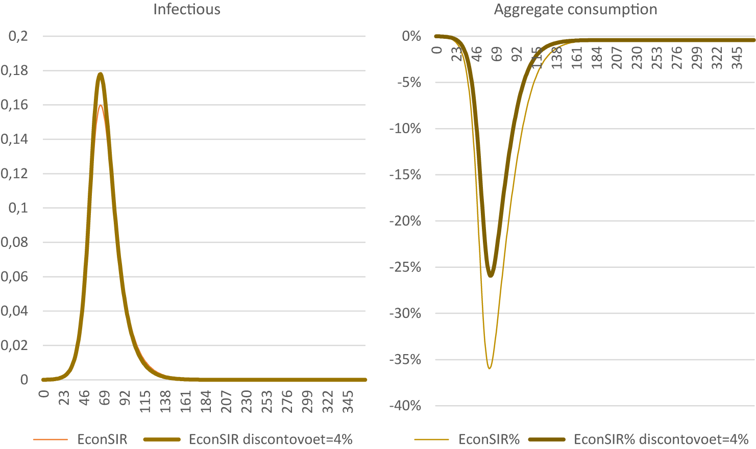
Figure C3. Using a 4 % discount rate. The horizontal axis is the number of days since the start of the pandemic.
C.3. Productivity loss of infected persons
The productivity loss of those infected (ϕI) is calibrated at 26 % for the Epi-econ model. A lower (20 %) or substantially higher (50 %) productivity loss when infected has a very limited effect on model outcomes (Figure C4). This is due to counteracting effects: on the one hand, a larger loss of productivity means that infected persons experience a larger consumption loss and a larger utility loss than in the original calibration. This implies that it becomes more costly for susceptible individuals to become infected. On the other hand, the reduced consumption of infected people also means that the probability of a susceptible person meeting an infected person reduces. Thus, the consequences of getting infected are more severe, but the probability of becoming infected is reduced (see Box C1 for details).
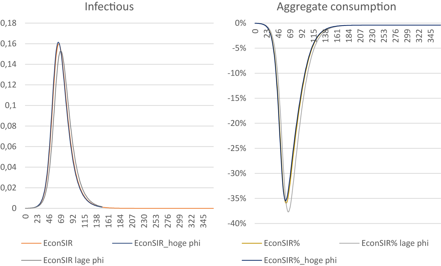
Figure C4. Using productivity when infected of 0.5 and 0.8. The horizontal axis is the number of days since the start of the pandemic.
Box C1. The influence of $ {\phi}^I $
on cs: an exercise in comparative statics.
$ {\phi}^I $
on cs: an exercise in comparative statics.
In this box, we analyze the effect of productivity loss of infected persons ϕI on the consumption of susceptibles cs using comparative statics. For simplicity, we do not consider policy: μt = Γt = 0. For notational convenience, we replace $ {\phi}^I $
by
$ {\phi}^I $
by $ \phi $
. It is useful to note that in this box, we analyze an increase in
$ \phi $
. It is useful to note that in this box, we analyze an increase in $ \phi $
(
$ \phi $
( $ d\phi $
>0), which amounts to higher productivity of infected persons and fewer hours lost due to illness. Furthermore, in this box, we refer to Lagrange multipliers (the λ’s). These reflect the shadow prices of the restrictions, such as budget constraints (λ
b for each consumer type S, I, or R) and the intertemporal restriction implied by the epidemic (λ
τ).
$ d\phi $
>0), which amounts to higher productivity of infected persons and fewer hours lost due to illness. Furthermore, in this box, we refer to Lagrange multipliers (the λ’s). These reflect the shadow prices of the restrictions, such as budget constraints (λ
b for each consumer type S, I, or R) and the intertemporal restriction implied by the epidemic (λ
τ).
First, we assess how $ \phi $
affects the behavior and utility of the infected persons. An infected person maximizes utility uI = ln(cI) – ½θ(nI)2 with a budget constraint cI = AnI. First-order conditions are nI = cI/
$ \phi $
affects the behavior and utility of the infected persons. An infected person maximizes utility uI = ln(cI) – ½θ(nI)2 with a budget constraint cI = AnI. First-order conditions are nI = cI/ $ \phi $
A, cI = 1/λbI en λbI = θnI/ϕA. This yields expressions for nI, cI, and λbI and their derivatives to ϕ:
$ \phi $
A, cI = 1/λbI en λbI = θnI/ϕA. This yields expressions for nI, cI, and λbI and their derivatives to ϕ:
 $$ {c}^I=\frac{\phi A}{\sqrt{\theta }}\Longrightarrow \frac{d{c}^I}{d\phi}=\frac{A}{\sqrt{\theta }},\hskip1em {n}^I=\frac{1}{\sqrt{\theta }}\Longrightarrow \frac{d{n}^I}{d\phi}=0,\hskip1em \mathrm{and}\hskip1em {\lambda}_b^I=\frac{1}{A\phi \sqrt{\theta }}\Longrightarrow \frac{d{\lambda}_b^I}{d\phi}=-\frac{1}{A{\phi}^2\sqrt{\theta }} $$
Rearranging implies that duI/dϕ = 1/ϕ. Lifetime utility UIt = uIt + β(1 – πr – πd)UI
t + 1 + βπr UR
t + 1 implies that $ \frac{d{U}_t^I}{d\phi}=\frac{1}{\phi \left[1-\beta \left(1-{\pi}_r-{\pi}_d\right)\right]}>0 $
is time independent (NB dUR/dϕ = 0). Using these insights, we turn to susceptibles. First-order conditions and their derivatives to ϕ are:
$ \frac{d{U}_t^I}{d\phi}=\frac{1}{\phi \left[1-\beta \left(1-{\pi}_r-{\pi}_d\right)\right]}>0 $
is time independent (NB dUR/dϕ = 0). Using these insights, we turn to susceptibles. First-order conditions and their derivatives to ϕ are:
 $$ \frac{1}{c^S}={\lambda}_b^S-{\lambda}_{\tau }{\pi}_1I{c}^I\Longrightarrow \frac{d{c}^S}{d\phi}=-{\left({c}^S\right)}^2\frac{d\frac{1}{c^S}}{d\phi}=-{\left({c}^S\right)}^2\left[\frac{d{\lambda}_b^S}{d\phi}-\frac{{d\lambda}_{\tau }}{d\phi}{\pi}_1I{c}^I-{\lambda}_{\tau }{\pi}_1I\frac{d{c}^I}{d\phi}\right], $$
 $$ \hskip-35em {n}^S=\frac{c^S}{A}\Longrightarrow \frac{d{n}^S}{d\phi}=\frac{1}{A}\frac{d{c}^S}{d\phi}, $$
 $$\begin{align} {\lambda}_b^S&=\frac{\theta {n}^S-{\lambda}_{\tau }{\pi}_2I{n}^I}{A}\Longrightarrow \frac{d{\lambda}_b^S}{d\phi}=\frac{\theta }{A}\frac{d{n}^S}{d\phi}=\frac{\theta }{A^2}\frac{d{c}^S}{d\phi},\hskip1em \mathrm{using}\frac{d{n}^I}{d\phi}=0\hskip1em \mathrm{and}\\
{\lambda}_{\tau }&=\beta \left({U}_{t+1}^I-{U}_{t+1}^S\right)\Longrightarrow \frac{d{\lambda}_{\tau }}{d\phi}=\frac{\beta }{\phi \left[1-\beta \left(1-{\pi}_r-{\pi}_d\right)\right]}-\beta \frac{{d U}_{t+1}^S}{d\phi}\end{align} $$
$$\begin{align} {\lambda}_b^S&=\frac{\theta {n}^S-{\lambda}_{\tau }{\pi}_2I{n}^I}{A}\Longrightarrow \frac{d{\lambda}_b^S}{d\phi}=\frac{\theta }{A}\frac{d{n}^S}{d\phi}=\frac{\theta }{A^2}\frac{d{c}^S}{d\phi},\hskip1em \mathrm{using}\frac{d{n}^I}{d\phi}=0\hskip1em \mathrm{and}\\
{\lambda}_{\tau }&=\beta \left({U}_{t+1}^I-{U}_{t+1}^S\right)\Longrightarrow \frac{d{\lambda}_{\tau }}{d\phi}=\frac{\beta }{\phi \left[1-\beta \left(1-{\pi}_r-{\pi}_d\right)\right]}-\beta \frac{{d U}_{t+1}^S}{d\phi}\end{align} $$
Substitution of the expression for $ \frac{d{\lambda}_b^S}{d\phi} $
in
$ \frac{d{\lambda}_b^S}{d\phi} $
in $ \frac{d{c}^S}{d\phi} $
yields
$ \frac{d{c}^S}{d\phi} $
yields $ \frac{d{c}^S}{d\phi}=-{\left({c}^S\right)}^2\frac{\theta }{A^2}\frac{d{c}^S}{d\phi}+{\left({c}^S\right)}^2\left[\frac{{d\lambda}_{\tau }}{d\phi}{\pi}_1I{c}^I+{\lambda}_{\tau }{\pi}_1I\frac{d{c}^I}{d\phi}\right] $
. Define
$ \frac{d{c}^S}{d\phi}=-{\left({c}^S\right)}^2\frac{\theta }{A^2}\frac{d{c}^S}{d\phi}+{\left({c}^S\right)}^2\left[\frac{{d\lambda}_{\tau }}{d\phi}{\pi}_1I{c}^I+{\lambda}_{\tau }{\pi}_1I\frac{d{c}^I}{d\phi}\right] $
. Define $ \sigma =\frac{{\left({c}^S\right)}^2}{1+{\left({c}^S\right)}^2\left(\frac{\theta }{A^2}\right)}>0 $
Footnote (a). It follows that
$ \sigma =\frac{{\left({c}^S\right)}^2}{1+{\left({c}^S\right)}^2\left(\frac{\theta }{A^2}\right)}>0 $
Footnote (a). It follows that $ \frac{d{c}^S}{d\phi}=\sigma [\frac{{d\lambda}_{\tau }}{d\phi}{\pi}_1I{c}^I+{\lambda}_{\tau }{\pi}_1I\frac{d{c}^I}{d\phi}] $
.
$ \frac{d{c}^S}{d\phi}=\sigma [\frac{{d\lambda}_{\tau }}{d\phi}{\pi}_1I{c}^I+{\lambda}_{\tau }{\pi}_1I\frac{d{c}^I}{d\phi}] $
.
The second term within the square brackets of this last expression shows how a change in the consumption of infected persons affects the consumption of susceptible people. This effect is negative because $ {\lambda}_{\tau }<0 $
. In other words, a higher ϕ leads to a higher consumption by infected persons (
$ {\lambda}_{\tau }<0 $
. In other words, a higher ϕ leads to a higher consumption by infected persons ( $ \frac{d{c}^I}{d\phi}=\frac{A}{\sqrt{\theta }}>0\Big) $
, which suppresses the consumption of susceptibles. And that, in turn, is because higher consumption of infected persons increases the likelihood of infection through the consumption channel, which will make susceptible people more cautious.
$ \frac{d{c}^I}{d\phi}=\frac{A}{\sqrt{\theta }}>0\Big) $
, which suppresses the consumption of susceptibles. And that, in turn, is because higher consumption of infected persons increases the likelihood of infection through the consumption channel, which will make susceptible people more cautious.
The first term within the square brackets shows that a higher ϕ reduces the expected loss of utility ( $ {\lambda}_{\tau }=\beta \left({U}_{t+1}^I-{U}_{t+1}^S\right) $
) due to infection (
$ {\lambda}_{\tau }=\beta \left({U}_{t+1}^I-{U}_{t+1}^S\right) $
) due to infection ( $ \frac{d{\lambda}_{\tau }}{d\phi}>0 $
). This stimulates the consumption of susceptibles as the cost of getting infected decreases.
$ \frac{d{\lambda}_{\tau }}{d\phi}>0 $
). This stimulates the consumption of susceptibles as the cost of getting infected decreases.
In short, a rise of ϕ increases the risk of becoming infected (cS ↓) but reduces the consequences (cS ↑). Which of these two counteracting effects dominates overall is an empirical matter. To our knowledge, conclusive empirical evidence is still lacking.
C.4. Removal rate
The removal rate is calibrated at 1/8, which signifies that an infected person stays infectious for 8 days on average and then recovers or dies. Figure C5 shows the effect of an increase in mean infectivity from 8 to 12 days, as assumed by Eichenbaum et al. (Reference Eichenbaum, Rebelo and Trabandt2021). A significant increase in peak prevalence results, while the economic effects are smaller. The reason for this is that although there are more infected persons, which increases the likelihood of becoming infected in general, but because infected persons work and consume less, the chance of getting infected while consuming or working is actually less.
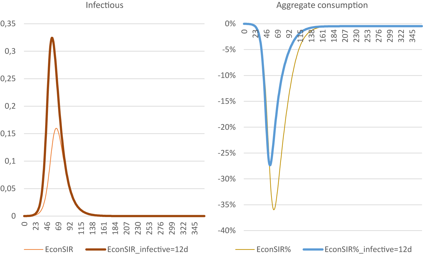
Figure C5. The effect of a longer infectious period (12 days instead of 8 days). The horizontal axis is the number of days since the start of the pandemic.
C.5. Case fatality rate
The CFR is calibrated at 0.5 %, c.q. Eichenbaum et al. (Reference Eichenbaum, Rebelo and Trabandt2021). A higher CFR reduces peak prevalence at the cost of a bigger recession (Figure C6). This is because the cost of contracting an infection is now greater and, therefore, people are scaling back their economic activities of their own accord.
Figure C6. The impact of a higher case fatality rate. The horizontal axis is the number of days since the start of the pandemic.
C.6. Disaggregation of endogenous effects and policy effects
Figure C7 shows the effects of (a) epi only, (b) Epi-econ and (c) Epi-econ + policy, with equal parameters otherwise. This allows gauging the relative contribution of policy on outcomes. Figure C7a shows that mean annual infections were 1.90, 1.71 and 0.35 %, respectively, indicating that policy contributed 87 % to the reduction in infectivity, and endogenous responses contributed 13 %. Figure C7b shows that mean annual consumption declined by −0.85, −4.62, and −13.50 %, respectively. This translates to policy contributing 70 % to economic decline and endogenous responses contributing 30 %.
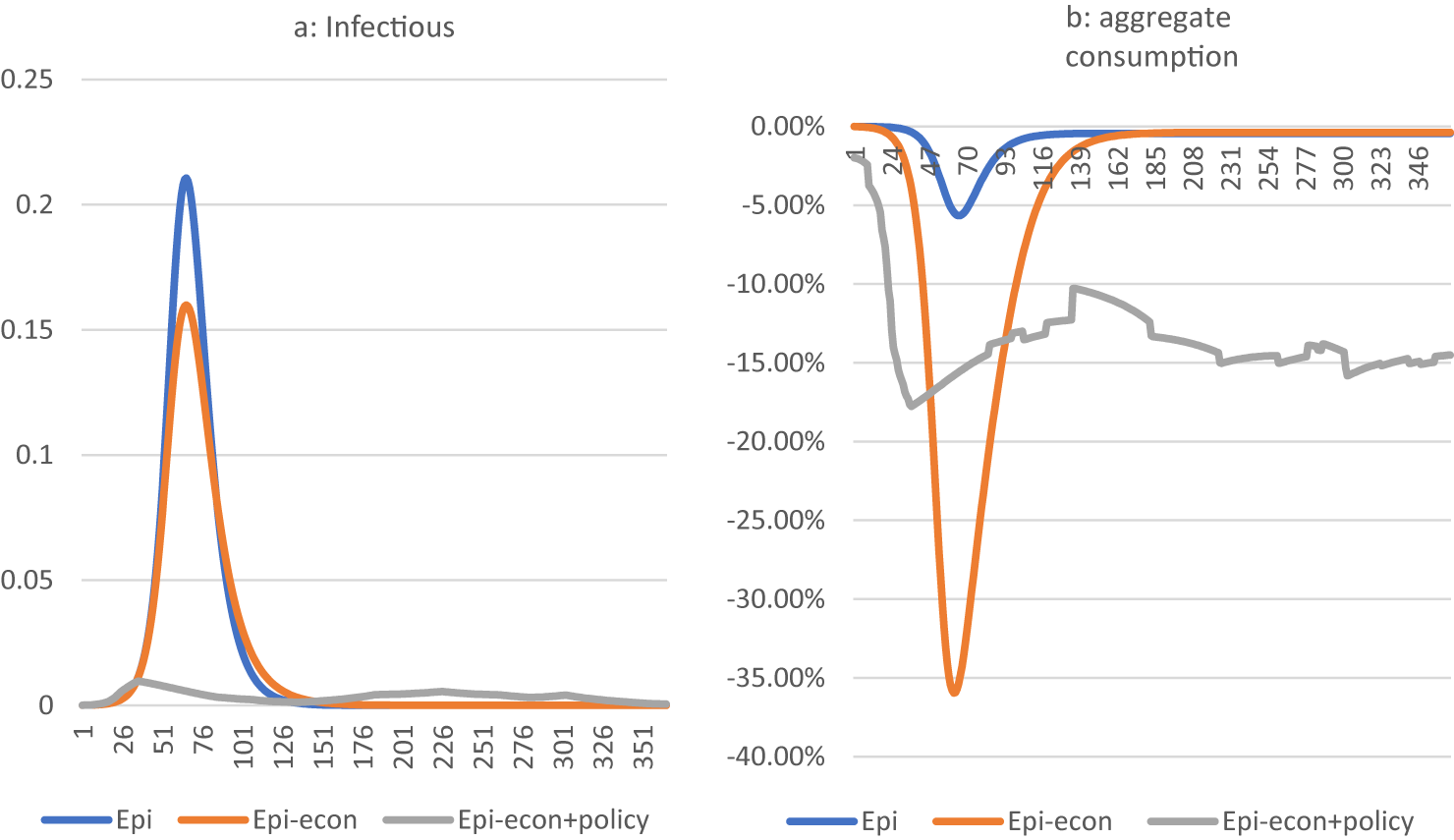
Figure C7. Simulation of the number of infectious people (a) and aggregate consumption (b), comparing the epi-model with the epi-econ model void of policy and the epi-econ model including policy measures .
D. Appendix D: nonlinear policy effects
To assess the effect of nonlinear policy effects at the margin, we evaluate the derivatives (dρ/dCHI) at CHI 2020 data mean, median, and double-sided 10 and 25 % intervals.
Table D1 suggests that, compared to the quadratic model, the linear model overstates effects of policy somewhat. It also interesting to note that the quadratic model hardly differentiates across the spectrum of policy interventions in terms of its effect on outcomes. Also interesting is that the exponential specification implies a slightly more responsive reaction of outcomes to policy and with responses higher at the higher end of the interventions. Differences are small across the spectrum. The different nonlinear approaches point to higher or lower elasticities compared to a linear model.
Table D1. Effect of CHI on ρ for different models at different positions in the frequency distribution of CHI
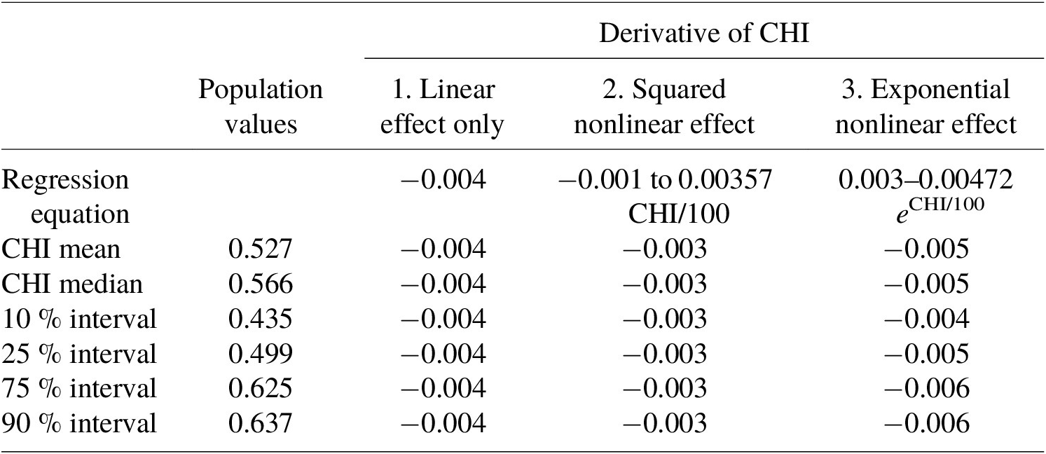


 Open access