


1. Introduction
Eddy viscosity and diffusivity models that are widely used in turbulence simulations are local in space and time. For example, in the eddy diffusivity model, the turbulent scalar flux at a point is assumed to be proportional to the mean scalar gradient at the same point. The local approximation requires the characteristic scale of the transport mechanism to be smaller than the distance over which the mean gradient of the transported property changes appreciably (Corrsin Reference Corrsin1974). However, the condition for the local approximation does not necessarily hold true for actual turbulent flows. A typical example is the scalar transport in the atmospheric boundary layer, where convective eddies driven by buoyancy are as large as the height of the boundary layer. Several attempts have been made to develop non-local models in addition to local eddy diffusivity models (Stull Reference Stull1984, Reference Stull1993; Ebert, Schumann & Stull Reference Ebert, Schumann and Stull1989; Pleim & Chang Reference Pleim and Chang1992). Berkowicz & Prahm (Reference Berkowicz and Prahm1980) proposed a generalisation of eddy diffusivity, which is the scalar flux expressed by a spatial integral of the mean scalar gradient. Romanof (Reference Romanof1989) studied space–time non-local models for turbulent diffusion, and Romanof (Reference Romanof2006) applied them to diffusion in atmospheric calm. In addition to scalar transport, non-local models have been developed for momentum transport. Nakayama & Vengadesan (Reference Nakayama and Vengadesan1993) proposed a non-local eddy viscosity model for the Reynolds stress. Egolf (Reference Egolf1994) developed a non-local model for the Reynolds stress called the difference-quotient turbulence model.
Recently, Mani & Park (Reference Mani and Park2021) developed the macroscopic forcing method to reveal the differential operators associated with turbulence closures. Using this method, Shirian & Mani (Reference Shirian and Mani2022) computed the scale-dependent eddy diffusivity characterising scalar and momentum transport and demonstrated that a non-local operator captures the eddy diffusivity behaviour. Liu, Williams & Mani (Reference Liu, Williams and Mani2023) developed a systematic and cost-effective approach for modelling the non-local eddy diffusivity using matched moment inverse operators. Lavacot et al. (Reference Lavacot, Liu, Williams, Morgan and Mani2024) investigated the non-locality of scalar transport in Rayleigh–Taylor instability using the macroscopic forcing method. Fractional calculus is another important method for investigating the non-local transport of turbulence. Fractional derivatives involve both differential and integral operators and can describe non-local properties (Uchaikin Reference Uchaikin2013). Non-local models for subgrid-scale viscosity and diffusivity in large-eddy simulations have been proposed using fractional operators (Samiee, Akhavan-Safaei & Zayernouri Reference Samiee, Akhavan-Safaei and Zayernouri2020; Di Leoni et al. Reference Di Leoni, Zaki, Karniadakis and Meneveau2021; Samiee, Akhavan-Safaei & Zayernouri Reference Samiee, Akhavan-Safaei and Zayernouri2022; Seyedi & Zayernouri Reference Seyedi and Zayernouri2022; Seyedi, Akhavan-Safae & Zayernouri Reference Seyedi, Akhavan-Safaei and Zayernouri2022). Di Leoni et al. (Reference Di Leoni, Zaki, Karniadakis and Meneveau2021) assessed the two-point correlation between the filtered strain rate and subfilter stress tensors to show that the non-local eddy viscosity model based on the fractional derivative accounts for long-tailed profiles of the correlation. Seyedi & Zayernouri (Reference Seyedi and Zayernouri2022) proposed a non-local subgrid-scale model for homogeneous isotropic turbulence using the fractional Laplacian operator and determined the fractional order using data-driven approaches. Reynolds-averaged Navier–Stokes (RANS) models have also been investigated using fractional derivatives. Fang et al. (Reference Fang, Sondak, Protopapas and Succi2020) applied the fractional derivative for the velocity gradient in neural-network models to represent the non-local property of the Reynolds stress in turbulent channel flow. Mehta (Reference Mehta2023) proposed fractional models for RANS equations by formulating a stress–strain relationship with variable-order fractional derivative.
Non-local expressions for momentum and scalar transport have also been investigated using the statistical theory of turbulence. Using the direct interaction approximation developed by Kraichnan (Reference Kraichnan1959), Roberts (Reference Roberts1961) studied turbulence diffusion to derive the probability distributions of the positions of fluid elements corresponding to non-local eddy diffusivity. Kraichnan (Reference Kraichnan1964) demonstrated that non-local eddy diffusivity can be approximated in terms of the averaged Green’s function and velocity correlation. Moreover, using Green’s functions for velocity and scalar fluctuations, Kraichnan (Reference Kraichnan1987) derived implicit exact non-local expressions for the Reynolds stress and scalar flux. Georgopoulos & Seinfeld (Reference Georgopoulos and Seinfeld1989) also derived a similar exact expression for the scalar flux. By modifying the Green’s function for scalar fluctuations, Hamba (Reference Hamba1995) derived an explicit exact non-local expression for scalar flux and evaluated non-local eddy diffusivity in the atmospheric convective boundary layer. A similar expression was investigated by Romanof (Reference Romanof1989) for a turbulent diffusion problem. Non-local eddy diffusivity and viscosity were evaluated, and the non-local expressions were verified using the direct numerical simulation (DNS) data of turbulent channel flow (Hamba Reference Hamba2004, Reference Hamba2005).
Recently, we examined a non-local expression for scalar flux in detail using a DNS of homogeneous isotropic turbulence with an inhomogeneous mean scalar (Hamba, Reference Hamba2022b ). We proposed a systematic model expression for non-local eddy diffusivity proportional to the two-point velocity correlation in a customary manner based on the statistical theory of turbulence (Kraichnan Reference Kraichnan1959; Yoshizawa Reference Yoshizawa1984, Reference Yoshizawa1998). In this model, the two-point velocity correlation is expressed in terms of the Kolmogorov energy spectrum. However, to apply the model to wall-bounded turbulence, we must replace the energy spectrum with a quantity in physical space. A candidate is the second-order structure function because its transport equation has been investigated not only in homogeneous isotropic turbulence, but also in inhomogeneous turbulence (Hill Reference Hill2002; Marati, Casciola & Piva Reference Marati, Casciola and Piva2004; Cimarelli et al. Reference Cimarelli, De Angelis and Casciola2013, Reference Cimarelli, De Angelis, Jiménez and Casciola2016; Gatti et al. Reference Gatti, Chiarini, Cimarelli and Quadrio2020). However, the behaviour of the structure function as the separation increases in an inhomogeneous direction is inadequate for turbulence modelling (Hamba Reference Hamba2023). Instead of the structure function, we recently proposed an expression for the scale-space energy density based on filtered velocities (Hamba, Reference Hamba2022a ). By adopting the scale-space energy density, we improved the non-local eddy diffusivity model and examined it using the DNS of homogeneous isotropic turbulence (Hamba Reference Hamba2023). In this paper, we examine non-local eddy diffusivity in detail using the DNS of turbulent channel flow. We modify the above model for non-local eddy diffusivity by incorporating the effects of turbulence anisotropy, inhomogeneity and wall boundaries to apply it to turbulent channel flow.
The remainder of this paper is organised as follows. In § 2, we evaluate the exact profiles of non-local eddy diffusivity using the DNS of turbulent channel flow. In § 3, we first describe the non-local eddy diffusivity model originally developed for homogeneous isotropic turbulence and then improve it for inhomogeneous turbulence. Using the new model, we evaluate the profiles of non-local eddy diffusivity and compare them with the DNS values to better understand non-local scalar transport in wall-bounded turbulence. Finally, § 4 presents our conclusions.
2. Analysis of non-local eddy diffusivity in channel flow
2.1. Non-local expression for turbulent scalar flux
We first describe an exact non-local expression for the turbulent scalar flux (Hamba Reference Hamba1995, Reference Hamba2004). The velocity $u_i^\ast$
and scalar
$u_i^\ast$
and scalar $\theta ^\ast$
are divided into mean and fluctuating parts as follows:
$\theta ^\ast$
are divided into mean and fluctuating parts as follows:
 \begin{align}& u_i^\ast =U_i+u_i,\ \ \ \ \ U_i= \langle u_i^\ast \rangle , \end{align}
 \begin{align}&\,\, \theta ^\ast =\Theta +\theta ,\ \ \ \ \ \Theta = \langle \theta ^\ast \rangle , \end{align}
where $\langle \;\rangle$
denotes ensemble averaging. A non-local expression for the turbulent scalar flux
$\langle \;\rangle$
denotes ensemble averaging. A non-local expression for the turbulent scalar flux $\langle u_i\theta \rangle$
can be expressed as
$\langle u_i\theta \rangle$
can be expressed as
 \begin{equation} \langle u_i\theta \rangle (\mathbf{x},t)=-\int {\mathrm{d}\mathbf{x}^\prime }\int _{-\infty }^{t}{\mathrm{d}t^\prime }\kappa _{NLij}(\mathbf{x},t;\mathbf{x}^\prime ,t^\prime )\frac {\partial }{\partial x_j^\prime }\Theta (\mathbf{x}^\prime ,t^\prime ) , \end{equation}
where $ \int \mathrm{d}\mathbf{x}=\int _{-\infty }^{\infty }\mathrm{d}x\int _{-\infty }^{\infty }\mathrm{d}y\int _{-\infty }^{\infty }\mathrm{d}z$
, and the summation convention is used for repeated indices. The velocity components should originally be written as
$ \int \mathrm{d}\mathbf{x}=\int _{-\infty }^{\infty }\mathrm{d}x\int _{-\infty }^{\infty }\mathrm{d}y\int _{-\infty }^{\infty }\mathrm{d}z$
, and the summation convention is used for repeated indices. The velocity components should originally be written as $u_1$
,
$u_1$
, $u_2$
and
$u_2$
and $u_3$
, but here they are written as
$u_3$
, but here they are written as $u_x$
,
$u_x$
, $u_y$
and
$u_y$
and $u_z$
instead. The same holds for
$u_z$
instead. The same holds for $\kappa _{NLij}$
. Here,
$\kappa _{NLij}$
. Here, $\kappa _{NLij}(\mathbf{x},t;\mathbf{x}^\prime ,t^\prime )$
is the non-local eddy diffusivity that represents the non-local effect of the mean scalar gradient at
$\kappa _{NLij}(\mathbf{x},t;\mathbf{x}^\prime ,t^\prime )$
is the non-local eddy diffusivity that represents the non-local effect of the mean scalar gradient at $(\mathbf{x}^\prime ,t^\prime )$
on the scalar flux at
$(\mathbf{x}^\prime ,t^\prime )$
on the scalar flux at $(\mathbf{x},t)$
. Using the Green’s function
$(\mathbf{x},t)$
. Using the Green’s function $g_j(\mathbf{x},t;\mathbf{x}^\prime ,t^\prime )$
for the scalar fluctuation equation, non-local eddy diffusivity is given by
$g_j(\mathbf{x},t;\mathbf{x}^\prime ,t^\prime )$
for the scalar fluctuation equation, non-local eddy diffusivity is given by
 \begin{equation} \kappa _{NLij}(\mathbf{x},t;\mathbf{x}^\prime ,t^\prime )=\langle u_i(\mathbf{x},t)g_j(\mathbf{x},t;\mathbf{x}^\prime ,t^\prime )\rangle . \end{equation}
A detailed description for the Green’s function is given in Appendix A.
Equation (2.3) was verified using the DNS data of turbulent channel flow and homogeneous isotropic turbulence (Hamba Reference Hamba2004, Reference Hamba2022b
). The non-local eddy diffusivity $\kappa _{NLij}(\mathbf{x},t;\mathbf{x}^\prime ,t^\prime )$
has a non-zero value if the distance
$\kappa _{NLij}(\mathbf{x},t;\mathbf{x}^\prime ,t^\prime )$
has a non-zero value if the distance $\left |\mathbf{x}-\mathbf{x}^\prime \right |$
and time difference
$\left |\mathbf{x}-\mathbf{x}^\prime \right |$
and time difference $t-t^\prime$
are comparable to or less than the turbulent length and time scales, respectively. If the mean scalar gradient
$t-t^\prime$
are comparable to or less than the turbulent length and time scales, respectively. If the mean scalar gradient $\partial \Theta /\partial x_j^\prime$
is nearly constant in this region in terms of space and time, then the scalar flux can be approximated as
$\partial \Theta /\partial x_j^\prime$
is nearly constant in this region in terms of space and time, then the scalar flux can be approximated as
 \begin{equation} \langle u_i\theta \rangle (\mathbf{x},t)=-\kappa _{Lij}(\mathbf{x},t)\frac {\partial \Theta }{\partial x_j} , \end{equation}
where $\kappa _{Lij}(\mathbf{x},t)$
is the local eddy diffusivity defined as
$\kappa _{Lij}(\mathbf{x},t)$
is the local eddy diffusivity defined as
 \begin{equation} \kappa _{Lij}(\mathbf{x},t)=\int {\mathrm{d}\mathbf{x}^\prime }\int _{-\infty }^{t}{\mathrm{d}t^\prime }\kappa _{NLij}(\mathbf{x},t;\mathbf{x}^\prime ,t^\prime ) . \end{equation}
Conversely, if the mean scalar gradient changes significantly in the region, the local approximation is invalid and the non-local expression should be used to predict the turbulent scalar flux.
2.2. Direct numerical simulation of turbulent channel flow
To investigate the behaviour of non-local eddy diffusivity in detail, we examined the DNS data of turbulent channel flow. The simulation was performed as follows. We numerically solved the equations for the velocity and scalar given by
 \begin{align}& \frac {\partial u_i^\ast }{\partial t}+\frac {\partial }{\partial x_j}u_j^\ast u_i^\ast =-\frac {\partial p^\ast }{\partial x_i}+\nu \frac {\partial ^2u_i^\ast }{\partial x_j\partial x_j}+f_u\delta _{i1} , \end{align}
 \begin{align}&\qquad\qquad\qquad\quad \frac {\partial u_i^\ast }{\partial x_i}=0 , \end{align}
 \begin{align}&\qquad\quad \frac {\partial \theta ^\ast }{\partial t}+\frac {\partial }{\partial x_i}u_i^\ast \theta ^\ast =\kappa \frac {\partial ^2\theta ^\ast }{\partial x_i\partial x_i}+f_\theta , \end{align}
where $p^\ast$
is the pressure,
$p^\ast$
is the pressure, $\nu$
is the molecular viscosity,
$\nu$
is the molecular viscosity, $\kappa$
is the molecular diffusivity,
$\kappa$
is the molecular diffusivity, $f_u(=1)$
is an external force and
$f_u(=1)$
is an external force and $f_\theta$
is an external source. In addition, we solved the equation for the Green’s function
$f_\theta$
is an external source. In addition, we solved the equation for the Green’s function $g_i(\mathbf{x},t;\mathbf{x}^\prime ,t^\prime )$
given by (A2). The size of the computational domain was
$g_i(\mathbf{x},t;\mathbf{x}^\prime ,t^\prime )$
given by (A2). The size of the computational domain was $L_x\times L_y\times L_z=3\pi \times 2\times 1.5\pi$
, where
$L_x\times L_y\times L_z=3\pi \times 2\times 1.5\pi$
, where $x$
,
$x$
, $y$
and
$y$
and $z$
denote the streamwise, wall-normal and spanwise directions, respectively. The number of grid points was
$z$
denote the streamwise, wall-normal and spanwise directions, respectively. The number of grid points was $N_x\times N_y\times N_z=256\times 128\times 256$
. The Reynolds number based on the friction velocity
$N_x\times N_y\times N_z=256\times 128\times 256$
. The Reynolds number based on the friction velocity $u_\tau$
and channel half-width
$u_\tau$
and channel half-width $L_y/2$
was set as
$L_y/2$
was set as ${Re}_\tau [=u_\tau (L_y/2)/\nu ]=180$
, and the Prandtl number was set as
${Re}_\tau [=u_\tau (L_y/2)/\nu ]=180$
, and the Prandtl number was set as $Pr(=\nu /\kappa )=1$
. Hereafter, the physical quantities are non-dimensionalised using
$Pr(=\nu /\kappa )=1$
. Hereafter, the physical quantities are non-dimensionalised using $u_\tau$
and
$u_\tau$
and $L_y/2$
. Periodic boundary conditions for
$L_y/2$
. Periodic boundary conditions for $u_i^\ast$
,
$u_i^\ast$
, $\theta ^\ast$
and
$\theta ^\ast$
and $g_i$
were used in the streamwise and spanwise directions, and the no-slip conditions
$g_i$
were used in the streamwise and spanwise directions, and the no-slip conditions $u_i^\ast =0$
,
$u_i^\ast =0$
, $\theta ^\ast =0$
and
$\theta ^\ast =0$
and $g_i=0$
were set at the wall at
$g_i=0$
were set at the wall at $y=\pm 1$
. We used the fourth-order finite-difference scheme in the
$y=\pm 1$
. We used the fourth-order finite-difference scheme in the $x$
and
$x$
and $z$
directions, the second-order scheme in the
$z$
directions, the second-order scheme in the $y$
direction and the Adams–Bashforth method for time marching. Statistical quantities were obtained by averaging over the
$y$
direction and the Adams–Bashforth method for time marching. Statistical quantities were obtained by averaging over the $x$
–
$x$
– $z$
plane and time.
$z$
plane and time.
We calculated two cases with respect to the scalar $\theta ^\ast$
; the profile of the external source
$\theta ^\ast$
; the profile of the external source $f_\theta$
was given by
$f_\theta$
was given by
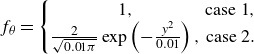 \begin{equation} f_\theta =\left \{\begin{matrix}1,&\textrm {case 1},\\\frac {2}{\sqrt {0.01\pi }}\exp \left (-\frac {y^2}{0.01}\right ),&\textrm {case 2}.\\\end{matrix}\right . \end{equation}
In case 1, the external source $f_\theta$
was constant in space, such as the external force
$f_\theta$
was constant in space, such as the external force $f_u$
for the velocity. In case 2,
$f_u$
for the velocity. In case 2, $f_\theta$
had a non-zero value only near the channel centre at
$f_\theta$
had a non-zero value only near the channel centre at $y=0$
. The integral value of
$y=0$
. The integral value of $f_\theta$
at
$f_\theta$
at $-1\leqslant y\leqslant 1$
was equal to 2 in both cases such that the mean scalar gradient at the wall could be equal to
$-1\leqslant y\leqslant 1$
was equal to 2 in both cases such that the mean scalar gradient at the wall could be equal to $1/\kappa$
. Similar profiles for the external sources were used in a previous study (Hamba Reference Hamba2004). Figure 1(a) shows the profiles of the mean velocity
$1/\kappa$
. Similar profiles for the external sources were used in a previous study (Hamba Reference Hamba2004). Figure 1(a) shows the profiles of the mean velocity $U_x$
and those of the mean scalar
$U_x$
and those of the mean scalar $\Theta$
for cases 1 and 2 as functions of
$\Theta$
for cases 1 and 2 as functions of $y^+[=(y+1)u_\tau /\nu ]$
. Because
$y^+[=(y+1)u_\tau /\nu ]$
. Because $f_\theta =f_u=1$
, the mean scalar profile in case 1 is nearly identical to the mean velocity profile. In contrast, the mean scalar profile in case 2 rapidly increases as
$f_\theta =f_u=1$
, the mean scalar profile in case 1 is nearly identical to the mean velocity profile. In contrast, the mean scalar profile in case 2 rapidly increases as $y$
increases near the channel centre at
$y$
increases near the channel centre at $y^+=180$
. Figure 1(b) shows the profiles of the mean scalar gradient as functions of
$y^+=180$
. Figure 1(b) shows the profiles of the mean scalar gradient as functions of $y$
for cases 1 and 2. The scalar gradient gradually decreases at
$y$
for cases 1 and 2. The scalar gradient gradually decreases at $-0.8\lt y\lt 0.8$
in case 1, whereas it rapidly decreases at
$-0.8\lt y\lt 0.8$
in case 1, whereas it rapidly decreases at $-0.1\lt y\lt 0.1$
in case 2. The length scale associated with the mean scalar gradient is large in case 1 and small near the channel centre in case 2.
$-0.1\lt y\lt 0.1$
in case 2. The length scale associated with the mean scalar gradient is large in case 1 and small near the channel centre in case 2.
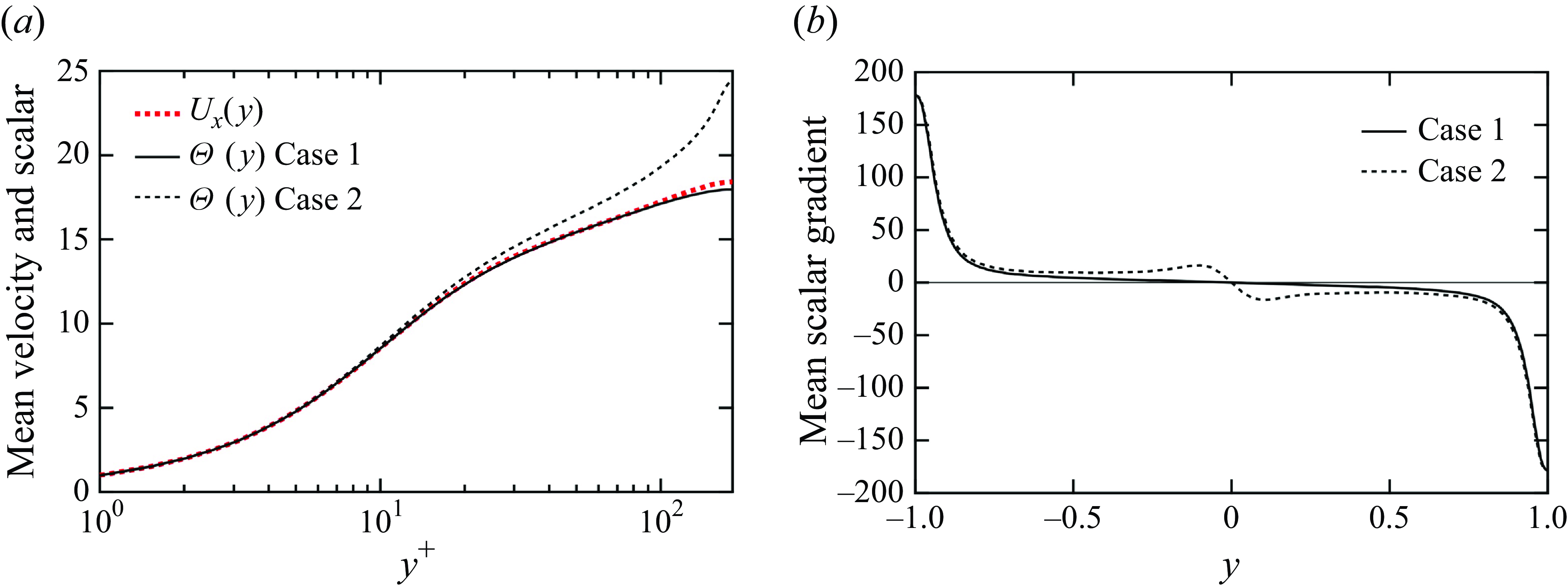
Figure 1. Profiles of the mean fields: (a) mean velocity $U_x$
and mean scalar
$U_x$
and mean scalar $\Theta$
for the two cases as functions of
$\Theta$
for the two cases as functions of $y^+$
, and (b) mean scalar gradient
$y^+$
, and (b) mean scalar gradient $\partial \Theta /\partial y$
as a function of
$\partial \Theta /\partial y$
as a function of $y$
for the two cases.
$y$
for the two cases.
2.3. Non-local eddy diffusivity evaluated using a DNS
Generally, non-local eddy diffusivity $\kappa _{NLij}$
is a function of
$\kappa _{NLij}$
is a function of $(\mathbf{x},t,\ \mathbf{x}^\prime ,t^\prime )$
. Because the turbulent field of channel flow is statistically steady and homogeneous in the
$(\mathbf{x},t,\ \mathbf{x}^\prime ,t^\prime )$
. Because the turbulent field of channel flow is statistically steady and homogeneous in the $x$
and
$x$
and $z$
directions, the non-local eddy diffusivity can be expressed as
$z$
directions, the non-local eddy diffusivity can be expressed as
 \begin{equation} \kappa _{NLij}(\mathbf{x},t;\mathbf{x}^\prime ,t^\prime )=\kappa _{NLij}(x-x^\prime ,y,y^\prime ,z-z^\prime ,\tau ) , \end{equation}
where $\tau =t-t^\prime$
. The wall-normal scalar flux is then given by a one-dimensional integral as
$\tau =t-t^\prime$
. The wall-normal scalar flux is then given by a one-dimensional integral as
 \begin{equation} \langle u_y\theta \rangle _{NL}(y)=-\int _{-1}^{1}{\mathrm{d}y^\prime }\kappa _{NLyy}(y,y^\prime )\frac {\partial \Theta }{\partial y^\prime } , \end{equation}
where
 \begin{equation} \kappa _{NLyy}(y,y^\prime )=\int _{0}^{3\pi }{\mathrm{d}x^\prime }\int _{0}^{1.5\pi }{\mathrm{d}z^\prime }\int _{0}^{\infty }\mathrm{d}\tau \kappa _{NLyy}(x-x^\prime ,y,y^\prime ,z-z^\prime ,\tau ) , \end{equation}
because the mean scalar gradient $\partial \Theta /\partial y^\prime$
depends only on
$\partial \Theta /\partial y^\prime$
depends only on $y'$
. The notation
$y'$
. The notation $\kappa _{NLyy}$
should originally be
$\kappa _{NLyy}$
should originally be $\kappa _{NL22}$
. Note that
$\kappa _{NL22}$
. Note that $\kappa _{NLyy}(y,y^\prime )$
on the left-hand side is a different quantity than
$\kappa _{NLyy}(y,y^\prime )$
on the left-hand side is a different quantity than $\kappa _{NLyy}(x-x^\prime ,y,y^\prime ,z-z^\prime ,\tau )$
on the right-hand side, although the same notation
$\kappa _{NLyy}(x-x^\prime ,y,y^\prime ,z-z^\prime ,\tau )$
on the right-hand side, although the same notation $\kappa _{NLyy}$
is used. They can be distinguished from the dimension of their input space. If
$\kappa _{NLyy}$
is used. They can be distinguished from the dimension of their input space. If $\partial \Theta /\partial y^\prime$
is nearly constant in the
$\partial \Theta /\partial y^\prime$
is nearly constant in the $y^\prime$
region where
$y^\prime$
region where $\kappa _{NLyy}(y,y^\prime )$
has a non-zero value, then the local approximation holds
$\kappa _{NLyy}(y,y^\prime )$
has a non-zero value, then the local approximation holds
 \begin{equation} \langle u_y\theta \rangle _{L}\left (y\right )=-\kappa _{Lyy}\left (y\right )\frac {\partial \Theta }{\partial y} , \end{equation}
where the local eddy diffusivity is defined as
 \begin{equation} \kappa _{Lyy}(y)=\int _{-1}^{1}{\mathrm{d}y^\prime }\kappa _{NLyy}(y,y^\prime ) . \end{equation}
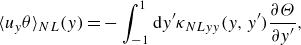
Figure 2. Profiles of non-local eddy diffusivity: (a) $\kappa _{NLyy}(y,y^\prime )$
as a function of
$\kappa _{NLyy}(y,y^\prime )$
as a function of $y$
and (b)
$y$
and (b) $\kappa _{NLyy}(y,y^\prime )$
as a function of
$\kappa _{NLyy}(y,y^\prime )$
as a function of $y^\prime$
.
$y^\prime$
.
Using results of the DNS described in § 2.2, we first examine the non-local eddy diffusivity $\kappa _{NLyy}(y,y^\prime )$
given by (2.13). The integrand
$\kappa _{NLyy}(y,y^\prime )$
given by (2.13). The integrand $\kappa _{NLyy}(x-x^\prime ,y,y^\prime ,z-z^\prime ,\tau )$
is given by (2.4), and the detailed method of its evaluation is described in Hamba (Reference Hamba2004). Note that the Green’s function
$\kappa _{NLyy}(x-x^\prime ,y,y^\prime ,z-z^\prime ,\tau )$
is given by (2.4), and the detailed method of its evaluation is described in Hamba (Reference Hamba2004). Note that the Green’s function $g_i(\mathbf{x},t;\mathbf{x}^\prime ,t^\prime )$
is obtained solely from the velocity field
$g_i(\mathbf{x},t;\mathbf{x}^\prime ,t^\prime )$
is obtained solely from the velocity field $u_i^\ast$
and the molecular diffusivity
$u_i^\ast$
and the molecular diffusivity $\kappa$
because the transport equation for
$\kappa$
because the transport equation for $g_i(\mathbf{x},t;\mathbf{x}^\prime ,t^\prime )$
given by (A2) does not involve the scalar
$g_i(\mathbf{x},t;\mathbf{x}^\prime ,t^\prime )$
given by (A2) does not involve the scalar $\theta ^\ast$
. Therefore, non-local eddy diffusivity is determined solely by the velocity field and the molecular diffusivity, and the same profile of non-local eddy diffusivity is applied to the scalar flux in cases 1 and 2.
$\theta ^\ast$
. Therefore, non-local eddy diffusivity is determined solely by the velocity field and the molecular diffusivity, and the same profile of non-local eddy diffusivity is applied to the scalar flux in cases 1 and 2.
Figure 2(a) shows the profiles of $\kappa _{NLyy}(y,y^\prime )$
as functions of
$\kappa _{NLyy}(y,y^\prime )$
as functions of $y$
for four locations of
$y$
for four locations of $y^\prime$
. The profiles represent the contribution to the scalar flux at
$y^\prime$
. The profiles represent the contribution to the scalar flux at $y$
from the mean scalar gradient at a given location of
$y$
from the mean scalar gradient at a given location of $y^\prime$
. The peak values of the profiles reflect the turbulence intensity
$y^\prime$
. The peak values of the profiles reflect the turbulence intensity $\langle u^{2}_{y}\rangle$
at
$\langle u^{2}_{y}\rangle$
at $y=y'$
. The peak value
$y=y'$
. The peak value $\kappa _{NLyy}(y,y)$
is correlated with
$\kappa _{NLyy}(y,y)$
is correlated with $\langle u_{y}^{2}\rangle (y)$
because
$\langle u_{y}^{2}\rangle (y)$
because $u_y(x,y,z,t)$
and
$u_y(x,y,z,t)$
and $u_y(x^\prime ,y,z^\prime ,t^\prime )$
are used to evaluate
$u_y(x^\prime ,y,z^\prime ,t^\prime )$
are used to evaluate $\kappa _{NLyy}(y,y)$
. As
$\kappa _{NLyy}(y,y)$
. As $y'$
increases, it increases rapidly and then decreases gradually towards the centre of the channel. The widths of the profiles reflect the extent of the non-local effect. The profile for
$y'$
increases, it increases rapidly and then decreases gradually towards the centre of the channel. The widths of the profiles reflect the extent of the non-local effect. The profile for $y^\prime =-0.942$
(
$y^\prime =-0.942$
( $y^{\prime +}=10.5$
), plotted as a solid line, is narrow because
$y^{\prime +}=10.5$
), plotted as a solid line, is narrow because $y^\prime$
is close to the wall. As
$y^\prime$
is close to the wall. As $y^\prime$
increases, the profile becomes wider; the profile for
$y^\prime$
increases, the profile becomes wider; the profile for $y^\prime =0$
(
$y^\prime =0$
( $y^{\prime +}=180$
) at the channel centre, plotted as a dot-dashed line, is as wide as the channel half-width at approximately
$y^{\prime +}=180$
) at the channel centre, plotted as a dot-dashed line, is as wide as the channel half-width at approximately $-0.5\lt y\lt 0.5$
and is symmetrical with respect to the centre. The profile for
$-0.5\lt y\lt 0.5$
and is symmetrical with respect to the centre. The profile for $y^\prime =-0.486$
(
$y^\prime =-0.486$
( $y^{\prime +}=92.5$
) is also wide and nearly symmetrical with respect to the peak location at
$y^{\prime +}=92.5$
) is also wide and nearly symmetrical with respect to the peak location at $y=y^\prime$
. Owing to the wall boundary conditions
$y=y^\prime$
. Owing to the wall boundary conditions $u_i=0$
and
$u_i=0$
and $g_i=0$
, non-local eddy diffusivity also vanishes at the wall at
$g_i=0$
, non-local eddy diffusivity also vanishes at the wall at $y=\pm 1$
and exhibits a small value near the wall. This condition results in asymmetric profiles of non-local eddy diffusivity for
$y=\pm 1$
and exhibits a small value near the wall. This condition results in asymmetric profiles of non-local eddy diffusivity for $y^\prime =-0.942$
and
$y^\prime =-0.942$
and $y^\prime =-0.737$
; the profile is wider at
$y^\prime =-0.737$
; the profile is wider at $y\gt y'$
than at
$y\gt y'$
than at $y\lt y'$
. Figure 2(b) shows the profiles of
$y\lt y'$
. Figure 2(b) shows the profiles of $\kappa _{NLyy}(y,y^\prime )$
as functions of
$\kappa _{NLyy}(y,y^\prime )$
as functions of $y^\prime$
for four locations of
$y^\prime$
for four locations of $y$
. In this case, the profiles represent the contribution from the mean scalar gradient at
$y$
. In this case, the profiles represent the contribution from the mean scalar gradient at $y^\prime$
to the scalar flux at a given location of
$y^\prime$
to the scalar flux at a given location of $y$
. For example, the wide profile for
$y$
. For example, the wide profile for $y=-0.486$
(
$y=-0.486$
( $y^+=92.5$
), plotted as a small dotted line, indicates that the scalar flux at
$y^+=92.5$
), plotted as a small dotted line, indicates that the scalar flux at $y=-0.486$
is affected by the mean scalar gradient in the bottom half of the channel at approximately
$y=-0.486$
is affected by the mean scalar gradient in the bottom half of the channel at approximately $-1\lt y^\prime \lt 0$
. The profiles in figure 2(b) are very similar to the corresponding ones in figure 2(a) but not identical. The differences between the two types of profiles are discussed later using two-dimensional profiles.
$-1\lt y^\prime \lt 0$
. The profiles in figure 2(b) are very similar to the corresponding ones in figure 2(a) but not identical. The differences between the two types of profiles are discussed later using two-dimensional profiles.
Using the profiles of $\kappa _{NLyy}(y,y^\prime )$
obtained from the DNS, we verify the non-local expression for the scalar flux given by (2.12) (Hamba Reference Hamba2004). Figure 3 shows the profiles of the scalar fluxes as functions of
$\kappa _{NLyy}(y,y^\prime )$
obtained from the DNS, we verify the non-local expression for the scalar flux given by (2.12) (Hamba Reference Hamba2004). Figure 3 shows the profiles of the scalar fluxes as functions of $y$
for both cases. Here, ‘DNS’ denotes
$y$
for both cases. Here, ‘DNS’ denotes $\langle u_y\theta \rangle$
evaluated directly, ‘Non-local’ denotes
$\langle u_y\theta \rangle$
evaluated directly, ‘Non-local’ denotes $\langle u_y\theta \rangle _{NL}$
given by (2.12) and ‘Local’ denotes
$\langle u_y\theta \rangle _{NL}$
given by (2.12) and ‘Local’ denotes $\langle u_y\theta \rangle _{L}$
given by (2.14). The profiles of
$\langle u_y\theta \rangle _{L}$
given by (2.14). The profiles of $\langle u_y\theta \rangle _{NL}$
plotted as solid lines agree with the DNS values in both cases. This agreement verifies the non-local expression for scalar flux given by (2.12). As shown in figure 3(a), the profile of
$\langle u_y\theta \rangle _{NL}$
plotted as solid lines agree with the DNS values in both cases. This agreement verifies the non-local expression for scalar flux given by (2.12). As shown in figure 3(a), the profile of $\langle u_y\theta \rangle _{L}$
almost agrees with the DNS value within
$\langle u_y\theta \rangle _{L}$
almost agrees with the DNS value within $-0.8\lt y\lt 0.8$
. The local approximation is reasonable because the mean scalar gradient in case 1 changes gradually within
$-0.8\lt y\lt 0.8$
. The local approximation is reasonable because the mean scalar gradient in case 1 changes gradually within $-0.8\lt y\lt 0.8$
, as shown in figure 1(b), and its length scale is larger than the width of the non-local eddy diffusivity
$-0.8\lt y\lt 0.8$
, as shown in figure 1(b), and its length scale is larger than the width of the non-local eddy diffusivity $\kappa _{NLyy}(y,y^\prime )$
shown in figure 2(b). In contrast, as shown in figure 3(b), the profile of
$\kappa _{NLyy}(y,y^\prime )$
shown in figure 2(b). In contrast, as shown in figure 3(b), the profile of $\langle u_y\theta \rangle _{L}$
significantly overpredicts the DNS value near the channel centre within
$\langle u_y\theta \rangle _{L}$
significantly overpredicts the DNS value near the channel centre within $-0.2\lt y\lt 0.2$
. The local approximation is invalid because the mean scalar gradient decreases rapidly, as shown in figure 1(b), and its length scale is smaller than the width of the non-local eddy diffusivity. In both cases, the profile of
$-0.2\lt y\lt 0.2$
. The local approximation is invalid because the mean scalar gradient decreases rapidly, as shown in figure 1(b), and its length scale is smaller than the width of the non-local eddy diffusivity. In both cases, the profile of $\langle u_y\theta \rangle _{L}$
slightly overpredicts the DNS value near the wall within
$\langle u_y\theta \rangle _{L}$
slightly overpredicts the DNS value near the wall within $-1\lt y\lt -0.8$
and
$-1\lt y\lt -0.8$
and $0.8\lt y\lt 1$
. This is because the mean scalar gradient changes rapidly near the wall in both cases.
$0.8\lt y\lt 1$
. This is because the mean scalar gradient changes rapidly near the wall in both cases.
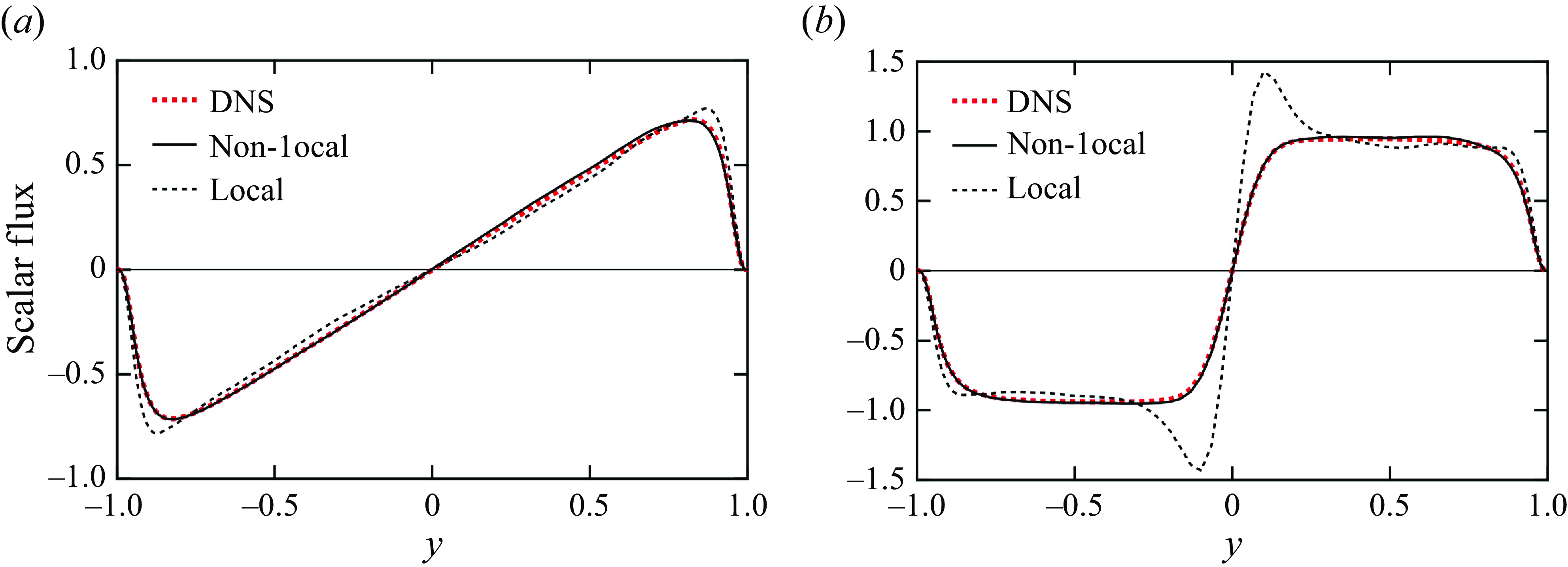
Figure 3. Profiles of the scalar fluxes $\langle u_y\theta \rangle$
,
$\langle u_y\theta \rangle$
, $\langle u_y\theta \rangle _{NL}$
and
$\langle u_y\theta \rangle _{NL}$
and $\langle u_y\theta \rangle _{L}$
as functions of
$\langle u_y\theta \rangle _{L}$
as functions of $y$
for (a) case 1 and (b) case 2.
$y$
for (a) case 1 and (b) case 2.
The profiles of non-local eddy diffusivity $\kappa _{NLyy}(y,y^\prime )$
are sufficient to verify the one-dimensional non-local expression given by (2.12). In this paper, to investigate non-local scalar transport in more detail, we further examine the non-local eddy diffusivity given by (2.13). Here, we consider the behaviour of non-local eddy diffusivity not only in the wall-normal direction but also in the streamwise direction. We can decompose the non-local eddy diffusivity
$\kappa _{NLyy}(y,y^\prime )$
are sufficient to verify the one-dimensional non-local expression given by (2.12). In this paper, to investigate non-local scalar transport in more detail, we further examine the non-local eddy diffusivity given by (2.13). Here, we consider the behaviour of non-local eddy diffusivity not only in the wall-normal direction but also in the streamwise direction. We can decompose the non-local eddy diffusivity $\kappa _{NLyy}(y,y^\prime )$
into the following integral in the streamwise direction:
$\kappa _{NLyy}(y,y^\prime )$
into the following integral in the streamwise direction:
 \begin{equation} \kappa _{NLyy}(y,y^\prime )=\int _{0}^{3\pi }{\mathrm{d}x^\prime }\kappa _{NLyy}(x-x^\prime ,y,y^\prime ) , \end{equation}
where
 \begin{equation} \kappa _{NLyy}(x-x^\prime ,y,y^\prime )=\int _{0}^{1.5\pi }{\mathrm{d}z^\prime }\int _{0}^{\infty }\mathrm{d}\tau \kappa _{NLyy}(x-x^\prime ,y,y^\prime ,z-z^\prime ,\tau ) . \end{equation}
Note that $\kappa _{NLyy}$
on the left-hand side is a different quantity than
$\kappa _{NLyy}$
on the left-hand side is a different quantity than $\kappa _{NLyy}$
on the right-hand side, although the same notation is used. The non-local eddy diffusivity
$\kappa _{NLyy}$
on the right-hand side, although the same notation is used. The non-local eddy diffusivity $\kappa _{NLyy}(x-x^\prime ,y,y^\prime )$
depends on both
$\kappa _{NLyy}(x-x^\prime ,y,y^\prime )$
depends on both $y$
and
$y$
and $y^\prime$
in the inhomogeneous wall-normal direction, whereas it depends only on the separation
$y^\prime$
in the inhomogeneous wall-normal direction, whereas it depends only on the separation $x-x^\prime$
in the homogeneous streamwise direction.
$x-x^\prime$
in the homogeneous streamwise direction.
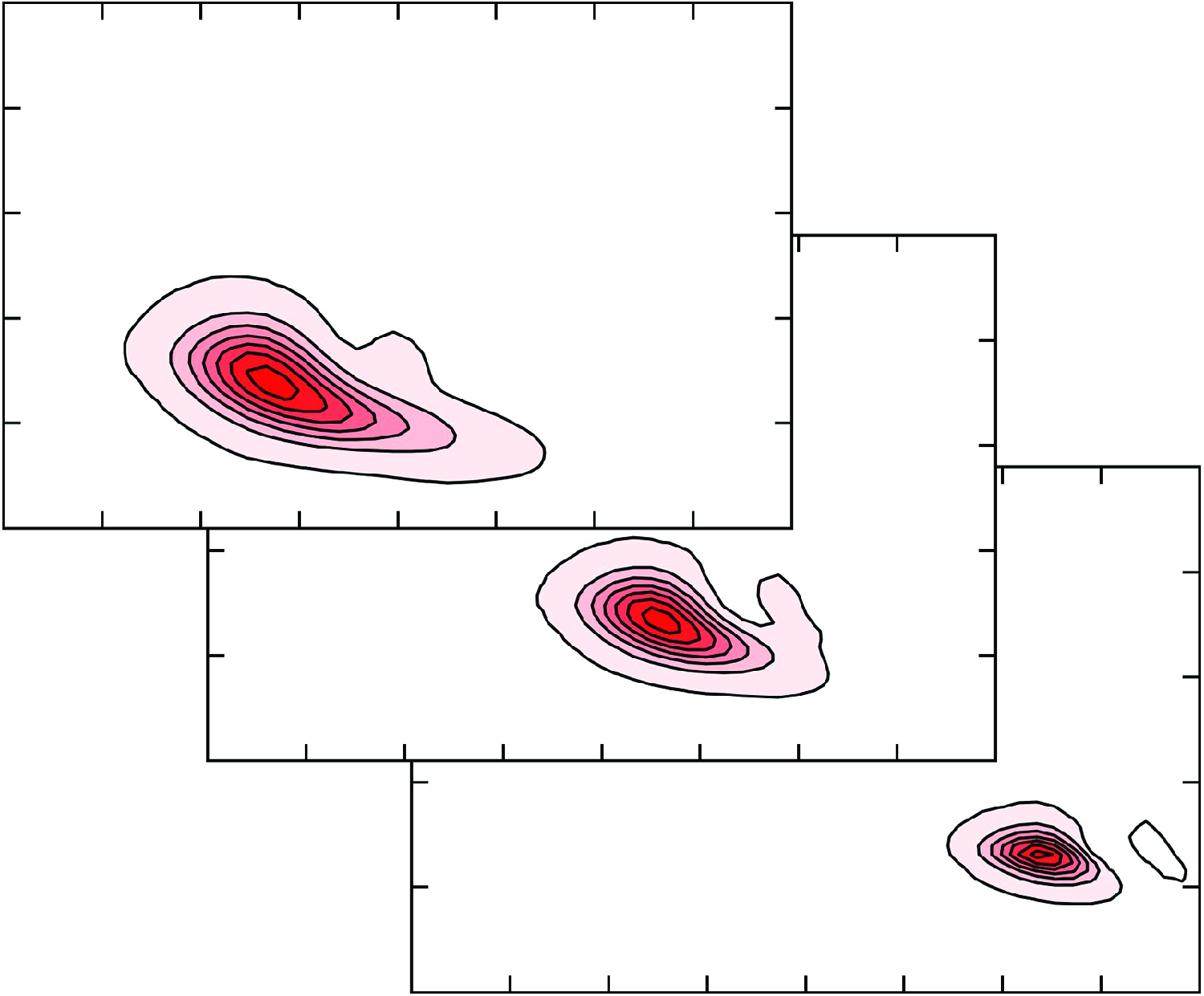
Figure 4(a) shows the two-dimensional contour plots of $\kappa _{NLyy}(x-x^\prime ,y,y^\prime )$
in the
$\kappa _{NLyy}(x-x^\prime ,y,y^\prime )$
in the $x-x^\prime$
and
$x-x^\prime$
and $y$
plane for
$y$
plane for $y^\prime =-0.737$
(
$y^\prime =-0.737$
( $y^{\prime +}=47.3$
). The position
$y^{\prime +}=47.3$
). The position $y^{\prime +}=47.3$
is located in the logarithmic layer of the turbulent channel flow. The profile represents the contribution to the scalar flux in the downstream region at
$y^{\prime +}=47.3$
is located in the logarithmic layer of the turbulent channel flow. The profile represents the contribution to the scalar flux in the downstream region at $(x-x^\prime ,y)$
from the mean scalar gradient at a given upstream location
$(x-x^\prime ,y)$
from the mean scalar gradient at a given upstream location $(x-x^\prime =0{,y=y}^\prime )$
. It appears as a typical profile of the diffusion of a scalar emitted from a point source; it spreads in the downstream direction by mean flow convection and in the wall-normal direction by turbulent diffusion. As shown in figure 2(a), the profile is slightly asymmetric with respect to the horizontal line at
$(x-x^\prime =0{,y=y}^\prime )$
. It appears as a typical profile of the diffusion of a scalar emitted from a point source; it spreads in the downstream direction by mean flow convection and in the wall-normal direction by turbulent diffusion. As shown in figure 2(a), the profile is slightly asymmetric with respect to the horizontal line at $y=y^\prime$
, and the contour is wider at
$y=y^\prime$
, and the contour is wider at $y\gt y^\prime$
than at
$y\gt y^\prime$
than at $y\lt y^\prime$
. Figure 4(b) shows the two-dimensional contour plots of
$y\lt y^\prime$
. Figure 4(b) shows the two-dimensional contour plots of $\kappa _{NLyy}(x-x^\prime ,y,y^\prime )$
in the
$\kappa _{NLyy}(x-x^\prime ,y,y^\prime )$
in the $x^\prime -x$
and
$x^\prime -x$
and $y^\prime$
plane for
$y^\prime$
plane for $y=-0.737$
(
$y=-0.737$
( $y^+=47.3$
). The profile represents the contribution from the mean scalar gradient in the upstream region at
$y^+=47.3$
). The profile represents the contribution from the mean scalar gradient in the upstream region at $(x^\prime -x,y^\prime )$
to the scalar flux at a given downstream location
$(x^\prime -x,y^\prime )$
to the scalar flux at a given downstream location $(x^\prime -x=0,y^\prime =y)$
. This indicates that the mean scalar gradient in a wide upstream region significantly affects the scalar flux at
$(x^\prime -x=0,y^\prime =y)$
. This indicates that the mean scalar gradient in a wide upstream region significantly affects the scalar flux at $(x^\prime -x=0,y^\prime =y)$
. The profile is similar to that shown in figure 4(a). However, the contribution from the bottom region at
$(x^\prime -x=0,y^\prime =y)$
. The profile is similar to that shown in figure 4(a). However, the contribution from the bottom region at $y^\prime \lt y$
is slightly larger in figure 4(b).
$y^\prime \lt y$
is slightly larger in figure 4(b).

Figure 4. Contour plots of non-local eddy diffusivity: (a) $\kappa _{NLyy}(x-x^\prime ,y,y^\prime )$
as a function of
$\kappa _{NLyy}(x-x^\prime ,y,y^\prime )$
as a function of $x-x^\prime$
and
$x-x^\prime$
and $y$
for
$y$
for $y^\prime =-0.737$
(
$y^\prime =-0.737$
( $y^{\prime +}=47.3$
) and (b)
$y^{\prime +}=47.3$
) and (b) $\kappa _{NLyy}(x-x^\prime ,y,y^\prime )$
as a function of
$\kappa _{NLyy}(x-x^\prime ,y,y^\prime )$
as a function of $x^\prime -x$
and
$x^\prime -x$
and $y^\prime$
for
$y^\prime$
for $y=-0.737$
(
$y=-0.737$
( $y^+=47.3$
).
$y^+=47.3$
).
Figure 5 shows the two-dimensional contour plots of $\kappa _{NLyy}(x-x^\prime ,y,y^\prime )$
for
$\kappa _{NLyy}(x-x^\prime ,y,y^\prime )$
for $y^\prime =-0.942$
(
$y^\prime =-0.942$
( $y^{\prime +}=10.5$
) and
$y^{\prime +}=10.5$
) and $y=-0.942$
(
$y=-0.942$
( $y^+=10.5$
). The position
$y^+=10.5$
). The position $y^{+}=10.5$
is located in the buffer layer of the turbulent channel flow, which is closer to the bottom wall than that in figure 4. In figure 5(a), because of the wall effect at
$y^{+}=10.5$
is located in the buffer layer of the turbulent channel flow, which is closer to the bottom wall than that in figure 4. In figure 5(a), because of the wall effect at $y=-1$
, the contour near the wall becomes nearly horizontal, and the profile is more asymmetric with respect to the horizontal line at
$y=-1$
, the contour near the wall becomes nearly horizontal, and the profile is more asymmetric with respect to the horizontal line at $y=y^\prime$
than in figure 4(a). The same holds for figure 5(b). Moreover, the contour in the streamwise direction is longer in figure 5(b) than in figure 5(a). In summary, the two-dimensional profiles of non-local eddy diffusivity clearly reveal a contribution from the mean scalar gradient in a wide upstream region to the scalar flux at a given location, which cannot be observed in the one-dimensional profiles in figure 2.
$y=y^\prime$
than in figure 4(a). The same holds for figure 5(b). Moreover, the contour in the streamwise direction is longer in figure 5(b) than in figure 5(a). In summary, the two-dimensional profiles of non-local eddy diffusivity clearly reveal a contribution from the mean scalar gradient in a wide upstream region to the scalar flux at a given location, which cannot be observed in the one-dimensional profiles in figure 2.
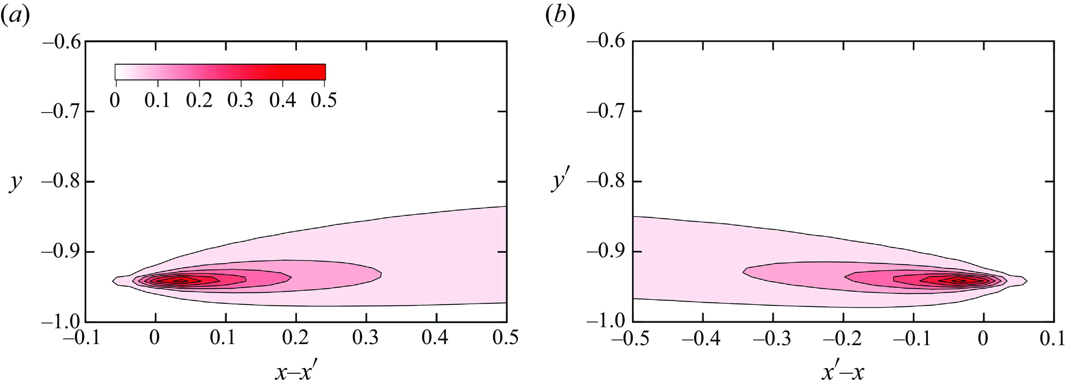
Figure 5. Contour plots of non-local eddy diffusivity: (a) $\kappa _{NLyy}(x-x^\prime ,y,y^\prime )$
as a function of
$\kappa _{NLyy}(x-x^\prime ,y,y^\prime )$
as a function of $x-x^\prime$
and
$x-x^\prime$
and $y$
for
$y$
for $y^\prime =-0.942$
(
$y^\prime =-0.942$
( $y^{\prime +}=10.5$
) and (b)
$y^{\prime +}=10.5$
) and (b) $\kappa _{NLyy}(x-x^\prime ,y,y^\prime )$
as a function of
$\kappa _{NLyy}(x-x^\prime ,y,y^\prime )$
as a function of $x^\prime -x$
and
$x^\prime -x$
and $y^\prime$
for
$y^\prime$
for $y=-0.942$
(
$y=-0.942$
( $y^+=10.5$
).
$y^+=10.5$
).
To investigate the temporal behaviour of non-local scalar transport, we further decompose the two-dimensional profiles of non-local eddy diffusivity into the following time integral:
 \begin{equation} \kappa _{NLyy}(x-x^\prime ,y,y^\prime )=\int _{0}^{\infty }\mathrm{d}\tau \kappa _{NLyy}(x-x^\prime ,y,y^\prime ,\tau ) , \end{equation}
where
 \begin{equation} \kappa _{NLyy}(x-x^\prime ,y,y^\prime ,\tau )=\int _{0}^{1.5\pi }{\mathrm{d}z^\prime }\kappa _{NLyy}(x-x^\prime ,y,y^\prime ,z-z^\prime ,\tau ) . \end{equation}
Note that $\kappa _{NLyy}$
on the left-hand side is a different quantity than
$\kappa _{NLyy}$
on the left-hand side is a different quantity than $\kappa _{NLyy}$
on the right-hand side, although the same notation is used. Figures 6(a)–6(c) show the two-dimensional contour plots of
$\kappa _{NLyy}$
on the right-hand side, although the same notation is used. Figures 6(a)–6(c) show the two-dimensional contour plots of $\kappa _{NLyy}(x-x^\prime ,y,y^\prime ,\tau )$
in the
$\kappa _{NLyy}(x-x^\prime ,y,y^\prime ,\tau )$
in the $x-x^\prime$
and
$x-x^\prime$
and $y$
plane for
$y$
plane for $y^\prime =-0.737$
(
$y^\prime =-0.737$
( $y^{\prime +}=47.3$
) at
$y^{\prime +}=47.3$
) at $\tau =0.0225$
, 0.045 and 0.0675. The profiles represent the contribution to the scalar flux at
$\tau =0.0225$
, 0.045 and 0.0675. The profiles represent the contribution to the scalar flux at $(x-x^\prime ,y,t+\tau )$
from the mean scalar gradient at a given location and time of
$(x-x^\prime ,y,t+\tau )$
from the mean scalar gradient at a given location and time of $(x-x^\prime =0,y=y^\prime ,t)$
. The turbulence time scale can be defined as
$(x-x^\prime =0,y=y^\prime ,t)$
. The turbulence time scale can be defined as $T=K/\varepsilon$
where
$T=K/\varepsilon$
where $K(=\langle u_i^2\rangle /2)$
is the turbulent kinetic energy and
$K(=\langle u_i^2\rangle /2)$
is the turbulent kinetic energy and $\varepsilon$
is its dissipation rate. Because the turbulence time scale
$\varepsilon$
is its dissipation rate. Because the turbulence time scale $T=0.330$
at
$T=0.330$
at $y=-0.737$
, the normalised value
$y=-0.737$
, the normalised value $\tau /T$
ranges from 0.0682 to 0.205. As the time difference
$\tau /T$
ranges from 0.0682 to 0.205. As the time difference $\tau$
increases, the profile moves forward in the downstream direction. The peak location at each time point can be understood as convection based on the mean velocity
$\tau$
increases, the profile moves forward in the downstream direction. The peak location at each time point can be understood as convection based on the mean velocity $U(y^\prime )(=15.3)$
. The location
$U(y^\prime )(=15.3)$
. The location $x-x^\prime =U(y^\prime )\tau$
becomes 0.344, 0.689 and 1.03 for
$x-x^\prime =U(y^\prime )\tau$
becomes 0.344, 0.689 and 1.03 for $\tau =0.0225$
, 0.045 and 0.0675, respectively, which almost agrees with the peak location in figures 6(a)–6(c). In addition, as
$\tau =0.0225$
, 0.045 and 0.0675, respectively, which almost agrees with the peak location in figures 6(a)–6(c). In addition, as $\tau$
increases, the peak value decreases rapidly and the size of the profile increases gradually. The contours are more elliptical than circular; they are elongated in the streamwise direction and tilted towards the bottom wall. This behaviour suggests anisotropic diffusion in the
$\tau$
increases, the peak value decreases rapidly and the size of the profile increases gradually. The contours are more elliptical than circular; they are elongated in the streamwise direction and tilted towards the bottom wall. This behaviour suggests anisotropic diffusion in the $x-x^\prime$
and
$x-x^\prime$
and $y$
plane. Figures 6(d)–6(f) show the two-dimensional contour plots of
$y$
plane. Figures 6(d)–6(f) show the two-dimensional contour plots of $\kappa _{NLyy}(x-x^\prime ,y,y^\prime ,\tau )$
in the
$\kappa _{NLyy}(x-x^\prime ,y,y^\prime ,\tau )$
in the $x^\prime -x$
and
$x^\prime -x$
and $y^\prime$
plane for
$y^\prime$
plane for $y=-0.737$
(
$y=-0.737$
( $y^+=47.3$
) for the three values of
$y^+=47.3$
) for the three values of $\tau$
. The profiles represent the contribution from the mean scalar gradient at
$\tau$
. The profiles represent the contribution from the mean scalar gradient at $(x^\prime -x,y^\prime ,t-\tau )$
to the scalar flux at a given location and time of
$(x^\prime -x,y^\prime ,t-\tau )$
to the scalar flux at a given location and time of $(x^\prime -x=0, y^\prime =y,t)$
. As
$(x^\prime -x=0, y^\prime =y,t)$
. As $\tau$
increases, the profile moves backward in the upstream direction. The peak location can be understood as convection based on the mean velocity, similar to that in figures 6(a)–6(c). The contours are also elongated in the streamwise direction and tilted towards the centre of the channel. Clearly, the profile in figure 6(f) is more significantly elongated than that in figure 6(d) for the same value of
$\tau$
increases, the profile moves backward in the upstream direction. The peak location can be understood as convection based on the mean velocity, similar to that in figures 6(a)–6(c). The contours are also elongated in the streamwise direction and tilted towards the centre of the channel. Clearly, the profile in figure 6(f) is more significantly elongated than that in figure 6(d) for the same value of $\tau$
. The profiles in figures 6(d)–6(f) indicate that the mean scalar gradient in a wide upstream region in the past affects the scalar flux at a point and at the present, and that the region becomes wider as the time difference
$\tau$
. The profiles in figures 6(d)–6(f) indicate that the mean scalar gradient in a wide upstream region in the past affects the scalar flux at a point and at the present, and that the region becomes wider as the time difference $\tau$
increases. When the profiles of
$\tau$
increases. When the profiles of $\kappa _{NLyy}(x-x^\prime ,y,y^\prime ,\tau )$
are integrated over time, the profiles of
$\kappa _{NLyy}(x-x^\prime ,y,y^\prime ,\tau )$
are integrated over time, the profiles of $\kappa _{NLyy}(x-x^\prime ,y,y^\prime )$
are restored, as shown in figure 4. In figure 4, the profiles are nearly symmetrical with respect to the horizontal line at
$\kappa _{NLyy}(x-x^\prime ,y,y^\prime )$
are restored, as shown in figure 4. In figure 4, the profiles are nearly symmetrical with respect to the horizontal line at $y=y'$
. Anisotropic and tilted profiles are observed only in the temporal behaviour shown in figure 6.
$y=y'$
. Anisotropic and tilted profiles are observed only in the temporal behaviour shown in figure 6.
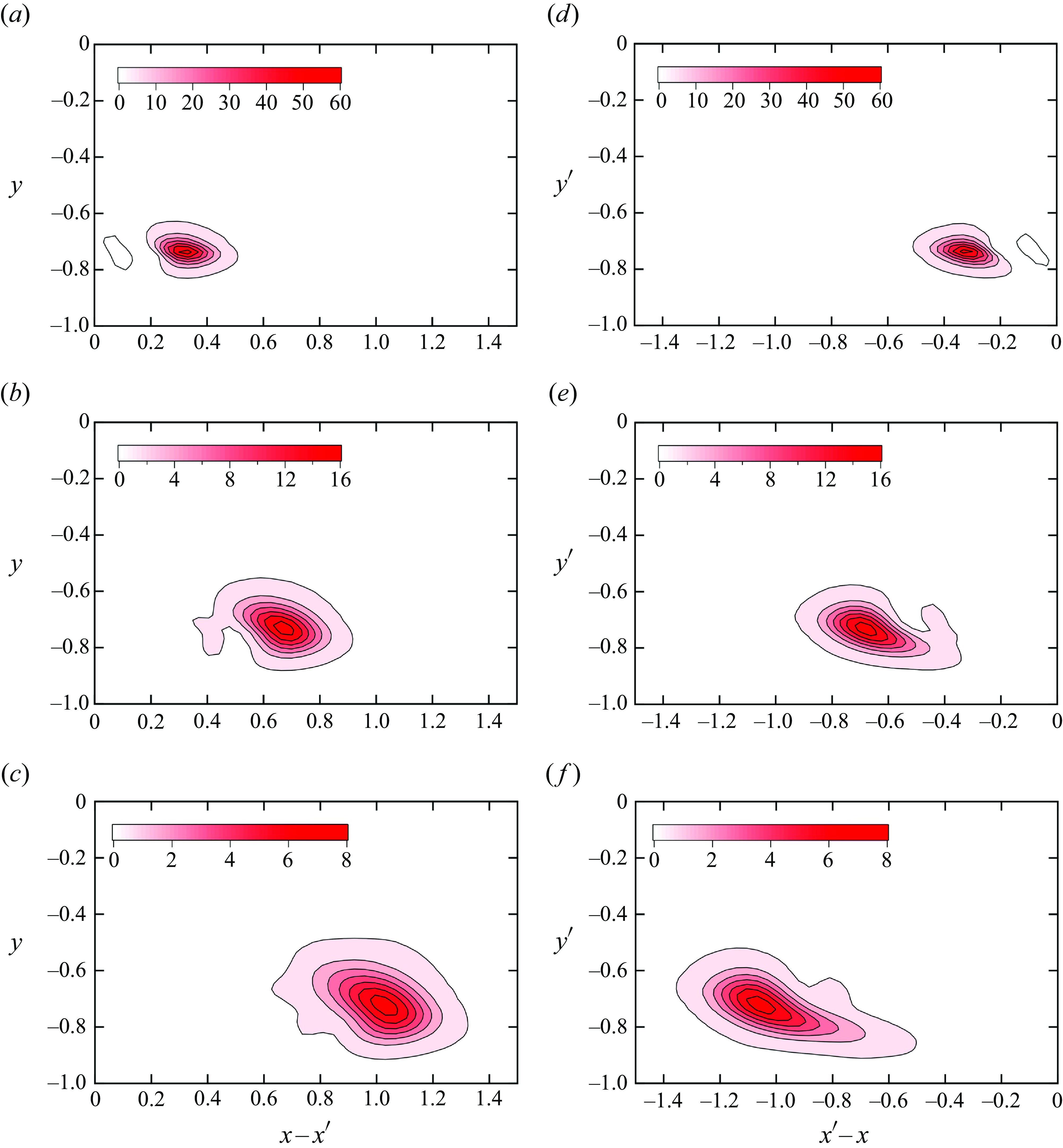
Figure 6. Contour plots of non-local eddy diffusivity: $\kappa _{NLyy}(x-x^\prime ,y,y^\prime ,\tau )$
as a function of
$\kappa _{NLyy}(x-x^\prime ,y,y^\prime ,\tau )$
as a function of $x-x^\prime$
and
$x-x^\prime$
and $y$
for
$y$
for $y^\prime =-0.737$
(
$y^\prime =-0.737$
( $y^{\prime +}=47.3$
) at (a)
$y^{\prime +}=47.3$
) at (a) $\tau =0.0225$
, (b)
$\tau =0.0225$
, (b) $\tau =0.045$
and (c)
$\tau =0.045$
and (c) $\tau =0.0675$
, and
$\tau =0.0675$
, and $\kappa _{NLyy}(x-x^\prime ,y,y^\prime ,\tau )$
as a function of
$\kappa _{NLyy}(x-x^\prime ,y,y^\prime ,\tau )$
as a function of $x^\prime -x$
and
$x^\prime -x$
and $y^\prime$
for
$y^\prime$
for $y=-0.737$
(
$y=-0.737$
( $y^+=47.3$
) at (d)
$y^+=47.3$
) at (d) $\tau =0.0225$
, (e)
$\tau =0.0225$
, (e) $\tau =0.045$
and (f)
$\tau =0.045$
and (f) $\tau =0.0675$
.
$\tau =0.0675$
.
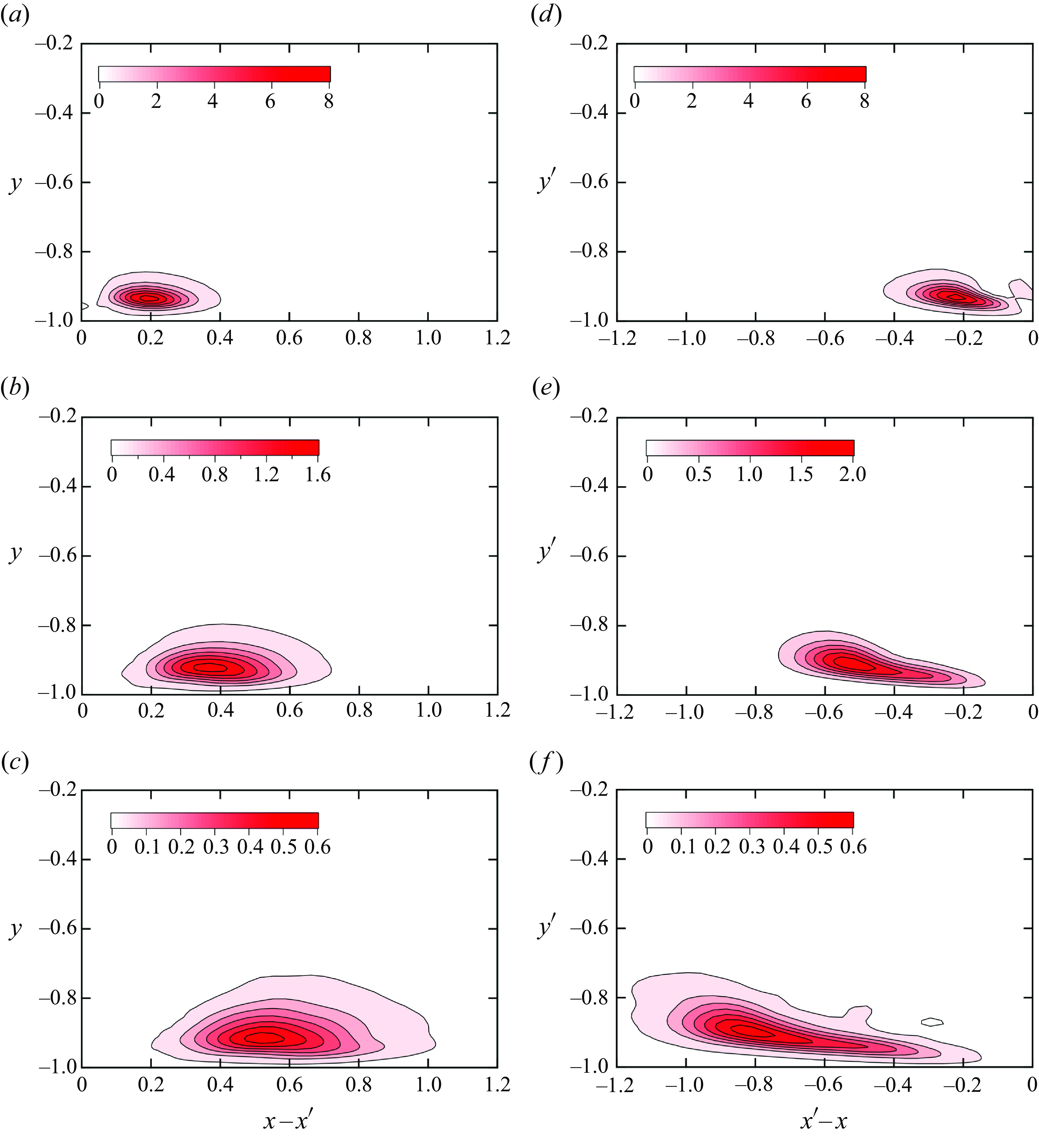
Figure 7. Contour plots of non-local eddy diffusivity: $\kappa _{NLyy}(x-x^\prime ,y,y^\prime ,\tau )$
as a function of
$\kappa _{NLyy}(x-x^\prime ,y,y^\prime ,\tau )$
as a function of $x-x^\prime$
and
$x-x^\prime$
and $y$
for
$y$
for $y^\prime =-0.942$
(
$y^\prime =-0.942$
( $y^{\prime +}=10.5$
) at (a)
$y^{\prime +}=10.5$
) at (a) $\tau =0.0225$
, (b)
$\tau =0.0225$
, (b) $\tau =0.045$
and (c)
$\tau =0.045$
and (c) $\tau =0.0675$
, and
$\tau =0.0675$
, and $\kappa _{NLyy}(x-x^\prime ,y,y^\prime ,\tau )$
as a function of
$\kappa _{NLyy}(x-x^\prime ,y,y^\prime ,\tau )$
as a function of $x^\prime -x$
and
$x^\prime -x$
and $y^\prime$
for
$y^\prime$
for $y=-0.942$
(
$y=-0.942$
( $y^+=10.5$
) at (d)
$y^+=10.5$
) at (d) $\tau =0.0225$
, (e)
$\tau =0.0225$
, (e) $\tau =0.045$
and (f)
$\tau =0.045$
and (f) $\tau =0.0675$
.
$\tau =0.0675$
.
Figures 7(a)–7(c) show the two-dimensional contour plots of $\kappa _{NLyy}(x-x^\prime ,y,y^\prime ,\tau )$
in the
$\kappa _{NLyy}(x-x^\prime ,y,y^\prime ,\tau )$
in the $x-x^\prime$
and
$x-x^\prime$
and $y$
plane for
$y$
plane for $y^\prime =-0.942$
(
$y^\prime =-0.942$
( $y^{\prime +}=10.5$
) for the three values of
$y^{\prime +}=10.5$
) for the three values of $\tau$
. Because the turbulence time scale is
$\tau$
. Because the turbulence time scale is $T=0.173$
at
$T=0.173$
at $y=-0.942$
, the normalised value
$y=-0.942$
, the normalised value $\tau /T$
ranges from 0.130 to 0.390. The peak location can also be understood as convection based on the mean velocity
$\tau /T$
ranges from 0.130 to 0.390. The peak location can also be understood as convection based on the mean velocity $U(y^\prime )(=8.82)$
. The location
$U(y^\prime )(=8.82)$
. The location $x-x^\prime =U(y^\prime )\tau$
becomes 0.198, 0.397 and 0.595 for
$x-x^\prime =U(y^\prime )\tau$
becomes 0.198, 0.397 and 0.595 for $\tau =0.0225$
, 0.045 and 0.0675, respectively, which almost agrees with the peak location in figures 7(a) and 7(b), whereas it slightly overpredicts the peak location in figure 7(c). The profiles are elongated in the streamwise direction, but they are not tilted towards the wall. Owing to the wall boundary conditions, non-local eddy diffusivity is limited to a small value near the wall, whereas the profile diffuses freely away from the wall. Figures 7(d)–7(f) show the two-dimensional contour plots of
$\tau =0.0225$
, 0.045 and 0.0675, respectively, which almost agrees with the peak location in figures 7(a) and 7(b), whereas it slightly overpredicts the peak location in figure 7(c). The profiles are elongated in the streamwise direction, but they are not tilted towards the wall. Owing to the wall boundary conditions, non-local eddy diffusivity is limited to a small value near the wall, whereas the profile diffuses freely away from the wall. Figures 7(d)–7(f) show the two-dimensional contour plots of $\kappa _{NLyy}(x-x^\prime ,y,y^\prime ,\tau )$
in the
$\kappa _{NLyy}(x-x^\prime ,y,y^\prime ,\tau )$
in the $x^\prime -x$
and
$x^\prime -x$
and $y^\prime$
plane for
$y^\prime$
plane for $y=-0.942$
(
$y=-0.942$
( $y^+=10.5$
) for the three values of
$y^+=10.5$
) for the three values of $\tau$
. As
$\tau$
. As $\tau$
increases, the profile moves backward in the upstream direction, similar to that in figures 6(d)–6(f). Compared with the profiles in figures 7(a)–7(c), the peak location moves faster, and the profiles are elongated more significantly. This behaviour accounts for the scenario in which the contour in the streamwise direction is longer in figure 5(b) than in figure 5(a). The profiles in figures 7(d)–7(f) also indicate a non-local contribution from the mean scalar gradient in a wide upstream region.
$\tau$
increases, the profile moves backward in the upstream direction, similar to that in figures 6(d)–6(f). Compared with the profiles in figures 7(a)–7(c), the peak location moves faster, and the profiles are elongated more significantly. This behaviour accounts for the scenario in which the contour in the streamwise direction is longer in figure 5(b) than in figure 5(a). The profiles in figures 7(d)–7(f) also indicate a non-local contribution from the mean scalar gradient in a wide upstream region.
In this section, we examine the one- and two-dimensional profiles of non-local eddy diffusivity obtained from the DNS. The two-dimensional profiles as functions of $x-x^\prime$
and
$x-x^\prime$
and $y$
in figures 4(a), 5(a), 6(a)–6(c) and 7(a)–7(c) show a forward diffusion process representing a contribution to the scalar flux at
$y$
in figures 4(a), 5(a), 6(a)–6(c) and 7(a)–7(c) show a forward diffusion process representing a contribution to the scalar flux at $(x-x^\prime ,y)$
. The temporal profile moves downstream, diffuses anisotropically and is tilted towards the bottom wall. The two-dimensional profiles as functions of
$(x-x^\prime ,y)$
. The temporal profile moves downstream, diffuses anisotropically and is tilted towards the bottom wall. The two-dimensional profiles as functions of $x^\prime -x$
and
$x^\prime -x$
and $y^\prime$
in figures 4(b), 5(b), 6(d)–6(f) and 7(d)–7(f) show a backward diffusion process representing a contribution from the mean scalar gradient at
$y^\prime$
in figures 4(b), 5(b), 6(d)–6(f) and 7(d)–7(f) show a backward diffusion process representing a contribution from the mean scalar gradient at $(x^\prime -x,y^\prime )$
. These profiles are directly related to the non-local expression given by (2.3) or the following two-dimensional expression
$(x^\prime -x,y^\prime )$
. These profiles are directly related to the non-local expression given by (2.3) or the following two-dimensional expression
 \begin{equation} \langle u_{y}\theta \rangle _{NL}(x,y)=-\int _{0}^{3\pi }{\mathrm{d}x^\prime }\int _{-1}^{1}{\mathrm{d}y^\prime }\kappa _{NLyy}(x-x^\prime ,y,y^\prime )\frac {\partial }{\partial y^\prime }\Theta (x^\prime ,y^\prime ) . \end{equation}
The temporal behaviour is similar to that of forward diffusion; however, the profiles are elongated more significantly in the streamwise direction. These results provide detailed information about non-local scalar transport, that is, how the mean scalar gradient affects the scalar flux non-locally in space and time.
3. Modelling non-local eddy diffusivity in channel flow
In § 2, the profiles of non-local eddy diffusivity are evaluated using the DNS of turbulent channel flow. In the analysis, we need to solve the equation for the Green’s function given by (A2). The profiles are exact in the sense that they satisfy the non-local expression for the turbulent scalar flux given by (2.3). However, the physical mechanisms that produce these profiles remain unclear. To better understand the behaviour of non-local eddy diffusivity and to accurately predict the scalar transport in the turbulence simulation, we attempt to develop a model for non-local eddy diffusivity. A model was developed for homogeneous isotropic turbulence and validated using the DNS (Hamba Reference Hamba2022b , Reference Hamba2023). In this paper, we improve it for inhomogeneous turbulence by incorporating the effects of turbulence anisotropy, inhomogeneity and wall boundaries. The model does not require solving the Green’s function equation; only the Reynolds stress and the energy dissipation rate are required. Because ensemble averaging is used to define the mean and fluctuating parts in (2.1) and (2.2), model expressions discussed in this study are for the RANS model. However, we expect that a similar non-local model can also be applied to the large-eddy simulation by adopting the filter width as a representative length scale.
3.1. Non-local eddy diffusivity model for homogeneous isotropic turbulence
In § 3.1, we briefly describe a model of non-local eddy diffusivity for homogeneous isotropic turbulence (Hamba Reference Hamba2022b , Reference Hamba2023). Because the turbulent velocity field is isotropic, non-local eddy diffusivity can be expressed in an isotropic form
 \begin{equation} \kappa _{NLij}(\mathbf{x},t;\mathbf{x}^\prime ,t^\prime )(\equiv \langle u_i(\mathbf{x},t)g_j(\mathbf{x},t;\mathbf{x}^\prime ,t^\prime )\rangle )=\kappa _{NL}(r,\tau )\delta _{ij} , \end{equation}
where $r=|\mathbf{r}|$
,
$r=|\mathbf{r}|$
, $\mathbf{r}=\mathbf{x}-\mathbf{x}^\prime$
and the term proportional to
$\mathbf{r}=\mathbf{x}-\mathbf{x}^\prime$
and the term proportional to $r_ir_j/r^2$
is neglected. Following the statistical theory of turbulence (Kraichnan Reference Kraichnan1964; Yoshizawa Reference Yoshizawa1998), we model the non-local eddy diffusivity
$r_ir_j/r^2$
is neglected. Following the statistical theory of turbulence (Kraichnan Reference Kraichnan1964; Yoshizawa Reference Yoshizawa1998), we model the non-local eddy diffusivity $\kappa _{NL} (r,\tau )$
using the two-point velocity correlation
$\kappa _{NL} (r,\tau )$
using the two-point velocity correlation $Q_{ii}(\mathbf{r})(=\langle u_i(\mathbf{x},t)u_i(\mathbf{x}^\prime ,t)\rangle )$
as
$Q_{ii}(\mathbf{r})(=\langle u_i(\mathbf{x},t)u_i(\mathbf{x}^\prime ,t)\rangle )$
as
 \begin{equation} \kappa _{NL}(r,\tau )=G(r,\tau )Q(r) , \end{equation}
where $Q(r)=Q_{ii}(\mathbf{r})/3$
.
$Q(r)=Q_{ii}(\mathbf{r})/3$
.
The time-dependent part $G(r,\tau )$
, which corresponds to the mean Green’s function for the scalar, is given by
$G(r,\tau )$
, which corresponds to the mean Green’s function for the scalar, is given by
 \begin{equation} G(r,\tau )=\frac {1}{(4\pi )^{3/2}(C_{\omega G}u_0\tau )^3}\exp \left [-\frac {r^2}{4(C_{\omega G}u_0\tau )^2}\right ] , \end{equation}
where $u_0=\langle u_i^2\rangle ^{1/2}=(2K)^{1/2}$
, and
$u_0=\langle u_i^2\rangle ^{1/2}=(2K)^{1/2}$
, and $C_{\omega G}(=0.46)$
is a model constant. Equation (3.3) represents a diffusion process with effective diffusivity
$C_{\omega G}(=0.46)$
is a model constant. Equation (3.3) represents a diffusion process with effective diffusivity $C_{\omega G}^2u_0^2\tau$
. Because it is multiplied by
$C_{\omega G}^2u_0^2\tau$
. Because it is multiplied by $Q(r)$
in (3.2), the magnitude of
$Q(r)$
in (3.2), the magnitude of $\kappa _{NL} (r,\tau )$
is proportional to
$\kappa _{NL} (r,\tau )$
is proportional to $Q(r)$
, and the region of diffusion is limited to the integral scale of turbulence even when
$Q(r)$
, and the region of diffusion is limited to the integral scale of turbulence even when $G(r,\tau )$
has a very wide profile for a large value of
$G(r,\tau )$
has a very wide profile for a large value of $\tau$
.
$\tau$
.
To model the velocity correlation $Q(r)$
, we use the energy density in the scale space developed by Hamba (Reference Hamba2022a
) instead of the energy spectrum in the wavenumber space. The velocity correlation
$Q(r)$
, we use the energy density in the scale space developed by Hamba (Reference Hamba2022a
) instead of the energy spectrum in the wavenumber space. The velocity correlation $Q_{ii}(\mathbf{r})$
can be expressed as the following integral with respect to the scale
$Q_{ii}(\mathbf{r})$
can be expressed as the following integral with respect to the scale $s$
:
$s$
:
 \begin{equation} Q_{ii}(\mathbf{r})=\int _{0}^{\infty }\mathrm{d}s{\hat {Q}}_{ii}(\mathbf{r},s) . \end{equation}
Here, ${\hat {Q}}_{ii}(\mathbf{r},s)$
is the velocity correlation in the scale space and is modelled in terms of the scale-space energy density
${\hat {Q}}_{ii}(\mathbf{r},s)$
is the velocity correlation in the scale space and is modelled in terms of the scale-space energy density ${\hat {Q}}_{ii}(s)$
and a simple Gaussian function as follows:
${\hat {Q}}_{ii}(s)$
and a simple Gaussian function as follows:
 \begin{equation} {\hat {Q}}_{ii}(\mathbf{r},s)={\hat {Q}}_{ii}(s)\exp \left (-\frac {r^2}{4s}\right ) . \end{equation}
For the scale-space energy density ${\hat {Q}}_{ii}(s)$
, we assume the following simple form:
${\hat {Q}}_{ii}(s)$
, we assume the following simple form:
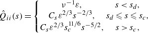 \begin{equation} {\hat {Q}}_{ii}(s)=\left \{\begin{matrix}\nu ^{-1}\varepsilon ,&s\lt s_d,\\C_s\varepsilon ^{2/3}s^{-2/3},&s_d\leqslant s\leqslant s_c,\\C_s\varepsilon ^{2/3}s_c^{11/6}s^{-5/2},&s\gt s_c,\\\end{matrix}\right . \end{equation}
where $C_s(=1.3)$
is a model constant, and two interface scales are introduced:
$C_s(=1.3)$
is a model constant, and two interface scales are introduced: $s_d(={C_s}^{3/2}\nu ^{3/2}\varepsilon ^{-1/2})$
in the dissipation range and
$s_d(={C_s}^{3/2}\nu ^{3/2}\varepsilon ^{-1/2})$
in the dissipation range and $s_c[=(6/11)^3{C_s}^{-3}K^3\varepsilon ^{-2}(1+{C_s}^{3/2}\nu ^{1/2}K^{-1}\varepsilon ^{1/2})^3]$
in the energy-containing range. The function
$s_c[=(6/11)^3{C_s}^{-3}K^3\varepsilon ^{-2}(1+{C_s}^{3/2}\nu ^{1/2}K^{-1}\varepsilon ^{1/2})^3]$
in the energy-containing range. The function $C_s\varepsilon ^{2/3}s^{-2/3}$
for
$C_s\varepsilon ^{2/3}s^{-2/3}$
for $s_d\leqslant s\leqslant s_c$
in (3.6) corresponds to the Kolmogorov energy spectrum
$s_d\leqslant s\leqslant s_c$
in (3.6) corresponds to the Kolmogorov energy spectrum $E(k)=C_K\varepsilon ^{2/3}k^{-5/3}$
. The filtered velocities are used to formulate the scale-space energy density (Hamba, Reference Hamba2022a
). A similar approach based on the filtered velocities was used to examine the roles of vorticity stretching and strain amplification in the turbulence energy cascade (Johnson Reference Johnson2020, Reference Johnson2021). A detailed description of the energy density and two-point velocity correlation in the scale space is given in Appendix B.
$E(k)=C_K\varepsilon ^{2/3}k^{-5/3}$
. The filtered velocities are used to formulate the scale-space energy density (Hamba, Reference Hamba2022a
). A similar approach based on the filtered velocities was used to examine the roles of vorticity stretching and strain amplification in the turbulence energy cascade (Johnson Reference Johnson2020, Reference Johnson2021). A detailed description of the energy density and two-point velocity correlation in the scale space is given in Appendix B.
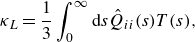
To understand the physical meaning of the non-local eddy diffusivity given by (3.2), we consider the local eddy diffusivity $\kappa _L$
corresponding to (2.15) as a simple case. The local approximation holds if the mean scalar gradient is nearly constant in space and time. For steady homogeneous isotropic turbulence, the local eddy diffusivity can be defined as
$\kappa _L$
corresponding to (2.15) as a simple case. The local approximation holds if the mean scalar gradient is nearly constant in space and time. For steady homogeneous isotropic turbulence, the local eddy diffusivity can be defined as
 \begin{equation} \kappa _L=\int \mathrm{d}\mathbf{r}\int _{0}^{\infty }\mathrm{d}\tau \kappa _{NL}(r,\tau ) . \end{equation}
Substituting (3.2) into (3.7) gives
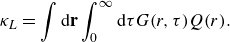 \begin{equation} \kappa _L=\int \mathrm{d}\mathbf{r}\int _{0}^{\infty }\mathrm{d}\tau G(r,\tau )Q(r) . \end{equation}
Furthermore, substituting (3.4) and (3.5) into (3.8) yields
 \begin{equation} \kappa _L=\frac {1}{3}\int _{0}^{\infty }\mathrm{d}s\hat {Q}_{ii} (s)T(s) , \end{equation}
where
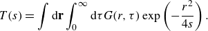 \begin{equation} T(s)=\int \mathrm{d}\mathbf{r}\int _{0}^{\infty }\mathrm{d}\tau G(r,\tau )\exp \left (-\frac {r^{2}}{4s}\right ) . \end{equation}
Here, $T(s)$
can be considered as the time scale of velocity fluctuations at scale
$T(s)$
can be considered as the time scale of velocity fluctuations at scale $s$
. Equation (3.9) suggests that the local eddy diffusivity can be obtained by summing the product of the turbulent energy
$s$
. Equation (3.9) suggests that the local eddy diffusivity can be obtained by summing the product of the turbulent energy $\hat {Q}_{ii}(s)$
and the time scale
$\hat {Q}_{ii}(s)$
and the time scale $T(s)$
over all scales. By focusing only on the large scales in the energy-containing range, we can derive a commonly used model
$T(s)$
over all scales. By focusing only on the large scales in the energy-containing range, we can derive a commonly used model
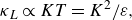 \begin{equation} \kappa _L\propto KT=K^2/\varepsilon , \end{equation}
where $T=K/\varepsilon$
is the turbulence time scale. Therefore, the model given by (3.9) is an extended model that accurately incorporates the effects of the turbulent energy and the time scale at each scale.
$T=K/\varepsilon$
is the turbulence time scale. Therefore, the model given by (3.9) is an extended model that accurately incorporates the effects of the turbulent energy and the time scale at each scale.
The model given by (3.8) can also be related to the integral length scale (Hamba, Reference Hamba2022b ). By substituting (3.3) into (3.8) and integrating it over time, we obtain
 \begin{equation} \kappa _L=\int _{0}^{\infty }\mathrm{d}r4\pi r^2\frac {1}{12\pi ^{3/2}C_{\omega G}u_0r^2}Q_{ii}(\mathbf{r}) =\frac {u_0}{3\pi ^{1/2}C_{\omega G}}\int _{0}^{\infty }\mathrm{d}r\frac {Q_{ii}(\mathbf{r})}{Q_{ii}(\mathbf{0})} . \end{equation}
The integral $\int _{0}^{\infty }\mathrm{d}rQ_{ii}(\mathbf{r})/Q_{ii}(\mathbf{0})$
appearing on the right-hand side can be considered as an integral length scale
$\int _{0}^{\infty }\mathrm{d}rQ_{ii}(\mathbf{r})/Q_{ii}(\mathbf{0})$
appearing on the right-hand side can be considered as an integral length scale $L$
. Equation (3.12) shows that the local eddy diffusivity is proportional to the product of the turbulent intensity
$L$
. Equation (3.12) shows that the local eddy diffusivity is proportional to the product of the turbulent intensity $u_0$
and the integral length scale
$u_0$
and the integral length scale $L$
; this relationship has been often discussed in turbulence model studies.
$L$
; this relationship has been often discussed in turbulence model studies.
3.2. Improvement of the model for inhomogeneous turbulence
The model expressions given by (3.2)–(3.6) were validated using the DNS of homogeneous isotropic turbulence with an inhomogeneous mean scalar in Hamba (Reference Hamba2023). In § 3.2, to apply it to turbulent channel flow, we improve the model by incorporating the effects of turbulence anisotropy, inhomogeneity and wall boundaries. Because the turbulent velocity field is statistically steady and homogeneous in the $x$
and
$x$
and $z$
directions, the model expression given by (3.2) can be rewritten as
$z$
directions, the model expression given by (3.2) can be rewritten as
 \begin{equation} \kappa _{NLij}(x-x^\prime ,y,y^\prime ,z-z^\prime ,\tau )=G(r_x,r_y,r_z,\tau ,y^\prime )Q_{ij}(r_x,r_y,r_z,y^\prime ) , \end{equation}
where $r_x=x-x^\prime -U_x(y^\prime )\tau$
,
$r_x=x-x^\prime -U_x(y^\prime )\tau$
, $r_y=y-y^\prime$
and
$r_y=y-y^\prime$
and $r_z=z-z^\prime$
. The effect of convection based on the mean velocity
$r_z=z-z^\prime$
. The effect of convection based on the mean velocity $U_x(y^\prime )$
is included in the definition of
$U_x(y^\prime )$
is included in the definition of $r_x$
. Owing to the inhomogeneity in the wall-normal direction, the coordinate
$r_x$
. Owing to the inhomogeneity in the wall-normal direction, the coordinate $y^\prime$
is included on the right-hand side of (3.13) in addition to
$y^\prime$
is included on the right-hand side of (3.13) in addition to $r_y$
.
$r_y$
.
In this study, we treat the wall-normal component given by
 \begin{equation} \kappa _{NLyy}(x-x^\prime ,y,y^\prime ,z-z^\prime ,\tau )=G(r_x,r_y,r_z,\tau ,y^\prime )Q_{yy}(r_x,r_y,r_z,y^\prime ) . \end{equation}
The anisotropy of the two-point velocity correlation $Q_{yy}(r_x,r_y,r_z,y^\prime )$
is expressed in terms of that of the Reynolds stress
$Q_{yy}(r_x,r_y,r_z,y^\prime )$
is expressed in terms of that of the Reynolds stress $R_{ij}(=\langle u_i u_j \rangle )$
at the
$R_{ij}(=\langle u_i u_j \rangle )$
at the $y^\prime$
location as follows:
$y^\prime$
location as follows:
 \begin{equation} Q_{yy}(r_x,r_y,r_z,y^\prime )=\frac {R_{yy}(y^\prime )}{R_{ii}(y^\prime )}Q_{jj}(r_x,r_y,r_z,y^\prime ) . \end{equation}
The correlation $Q_{jj}(r_x,r_y,r_z,y^\prime )$
is given by (3.4)–(3.6), and the values of
$Q_{jj}(r_x,r_y,r_z,y^\prime )$
is given by (3.4)–(3.6), and the values of $K$
and
$K$
and $\varepsilon$
included in (3.6) are evaluated at the
$\varepsilon$
included in (3.6) are evaluated at the $y^\prime$
location.
$y^\prime$
location.
The anisotropic effect of diffusion is incorporated into the time-dependent part $G(r,\tau )$
given by (3.3) using the Reynolds stress
$G(r,\tau )$
given by (3.3) using the Reynolds stress $R_{ij}(y')$
as follows (Roberts Reference Roberts1961):
$R_{ij}(y')$
as follows (Roberts Reference Roberts1961):
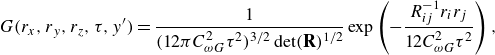 \begin{equation} G(r_x,r_y,r_z,\tau ,y^\prime )=\frac {1}{(12\pi C_{\omega G}^2\tau ^2)^{3/2}\det (\mathbf{R})^{1/2}}\exp \left (-\frac {R_{ij}^{-1}r_ir_j}{12C_{\omega G}^2\tau ^2}\right ) , \end{equation}
where
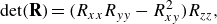 \begin{align}&\qquad\qquad\qquad\quad \det (\mathbf{R})=(R_{xx}R_{yy}-R_{xy}^2)R_{zz} , \end{align}
 \begin{align}& R_{ij}^{-1}r_ir_j=\frac {1}{R_{xx}R_{yy}-R_{xy}^2}(R_{yy}r_x^2-2R_{xy}r_xr_y+R_{xx}r_y^2)+\frac {1}{R_{zz}}r_z^2 . \end{align}
This form represents anisotropic diffusion, in which a scalar diffuses more quickly in the direction in which the Reynolds stress component is larger. Moreover, the Reynolds stress $R_{ij}$
included in (3.16)–(3.18) is replaced by
$R_{ij}$
included in (3.16)–(3.18) is replaced by $R_{ij}+\kappa /(3C_{\omega G}^2\tau )\delta _{ij}$
to incorporate the molecular diffusion effect for a very small value of
$R_{ij}+\kappa /(3C_{\omega G}^2\tau )\delta _{ij}$
to incorporate the molecular diffusion effect for a very small value of $\tau$
(see Appendix C for details).
$\tau$
(see Appendix C for details).
The wall boundary conditions must be considered for turbulent channel flow. Because $u_i=0$
and
$u_i=0$
and $g_j=0$
at the wall, the non-local eddy diffusivity given by (2.4) should also vanish at the wall. In this paper, the method of images is utilised to satisfy the wall boundary conditions. For example, the time-dependent part
$g_j=0$
at the wall, the non-local eddy diffusivity given by (2.4) should also vanish at the wall. In this paper, the method of images is utilised to satisfy the wall boundary conditions. For example, the time-dependent part $G(r_x,r_y,r_z,\tau ,y^\prime )$
near the bottom wall at
$G(r_x,r_y,r_z,\tau ,y^\prime )$
near the bottom wall at $y=-1$
can be modified as follows:
$y=-1$
can be modified as follows:
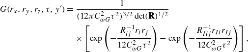 \begin{align} G(r_x,r_y,r_z,\tau ,y^\prime )&=\frac {1}{(12\pi C_{\omega G}^2\tau ^2)^{3/2}\det (\mathbf{R})^{1/2}}\notag \\ &\quad\times \left [\exp \left (-\frac {R_{ij}^{-1}r_ir_j}{12C_{\omega G}^2\tau ^2}\right )-\exp \left (-\frac {R_{Iij}^{-1}r_{Ii}r_{Ij}}{12C_{\omega G}^2\tau ^2}\right )\right ] , \end{align}
where $r_{Ix}=r_{x}$
,
$r_{Ix}=r_{x}$
, $r_{Iy}=y+2+y^\prime$
,
$r_{Iy}=y+2+y^\prime$
, $r_{Iz}=r_{z}$
,
$r_{Iz}=r_{z}$
, $R_{Ixx}=R_{xx}$
,
$R_{Ixx}=R_{xx}$
, $R_{Iyy}=R_{yy}$
,
$R_{Iyy}=R_{yy}$
, $R_{Izz}=R_{zz}$
and
$R_{Izz}=R_{zz}$
and $R_{Ixy}=-R_{xy}$
. Here, a negative point source of the diffusion is added at
$R_{Ixy}=-R_{xy}$
. Here, a negative point source of the diffusion is added at $(x',-2-y^\prime ,\ z')$
such that the value of
$(x',-2-y^\prime ,\ z')$
such that the value of $G(r_x,r_y,r_z,\tau ,y^\prime )$
vanishes at
$G(r_x,r_y,r_z,\tau ,y^\prime )$
vanishes at $y=-1$
. Similarly, the two-point velocity correlation
$y=-1$
. Similarly, the two-point velocity correlation $Q_{ii}(r_x,r_y,r_z,y^\prime )$
near the bottom wall is modified as
$Q_{ii}(r_x,r_y,r_z,y^\prime )$
near the bottom wall is modified as
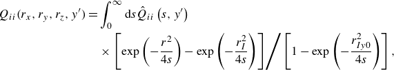 \begin{align} Q_{ii}(r_x,r_y,r_z,y^\prime )&=\int _{0}^{\infty }\mathrm{d}s{\hat {Q}}_{ii}\left (s,y^\prime \right )\notag \\ &\quad\times \left . \left [\exp \left (-\frac {r^2}{4s}\right )-\exp \left (-\frac {r_I^2}{4s}\right )\right ] \right / \left [1-\exp \left (-\frac {r_{Iy0}^2}{4s}\right )\right ] , \end{align}
where $r_I^2=r_{Ii}^2$
and
$r_I^2=r_{Ii}^2$
and $r_{Iy0}=2+{2y}^\prime$
. A factor
$r_{Iy0}=2+{2y}^\prime$
. A factor $[1-\exp (-r_{Iy0}^2/4s)]^{-1}$
is introduced in (3.20) such that for
$[1-\exp (-r_{Iy0}^2/4s)]^{-1}$
is introduced in (3.20) such that for $\mathbf{r}=\mathbf{0}$
, the turbulent kinetic energy can be expressed as the following integral of the scale-space energy density:
$\mathbf{r}=\mathbf{0}$
, the turbulent kinetic energy can be expressed as the following integral of the scale-space energy density:
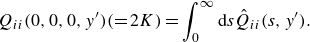 \begin{equation} Q_{ii}(0,0,0,y^\prime )(=2K)=\int _{0}^{\infty }\mathrm{d}s{\hat {Q}}_{ii}(s,y^\prime ) . \end{equation}
The form of the energy density ${\hat {Q}}_{ii}(s,y^\prime )$
given by (3.6) is a reasonable approximation for homogeneous isotropic turbulence (Hamba Reference Hamba2023); however, its accuracy for turbulent channel flow is not clear. The profiles of the scale-space energy density were evaluated for turbulent channel flow in Hamba (Reference Hamba2022a
). Figure 8 shows the profiles of the pre-multiplied energy density
${\hat {Q}}_{ii}(s,y^\prime )$
given by (3.6) is a reasonable approximation for homogeneous isotropic turbulence (Hamba Reference Hamba2023); however, its accuracy for turbulent channel flow is not clear. The profiles of the scale-space energy density were evaluated for turbulent channel flow in Hamba (Reference Hamba2022a
). Figure 8 shows the profiles of the pre-multiplied energy density ${s\hat {Q}}_{ii}(s,y)$
obtained from the DNS of the turbulent channel flow at
${s\hat {Q}}_{ii}(s,y)$
obtained from the DNS of the turbulent channel flow at ${Re}_\tau =590$
as a function of
${Re}_\tau =590$
as a function of $s$
at different
$s$
at different $y^+$
locations. The model profile reasonably agrees with the DNS value for
$y^+$
locations. The model profile reasonably agrees with the DNS value for $y^+=180$
and 490, but it underpredicts the DNS value at a large scale
$y^+=180$
and 490, but it underpredicts the DNS value at a large scale $s$
for
$s$
for $y^+=10$
and 50. In addition, we observe that the DNS value of the energy density for
$y^+=10$
and 50. In addition, we observe that the DNS value of the energy density for $y^+\lt 10$
has a profile similar to that for
$y^+\lt 10$
has a profile similar to that for $y^+=10$
whereas the model underpredicts it significantly. We then modify the scale-space energy density as follows:
$y^+=10$
whereas the model underpredicts it significantly. We then modify the scale-space energy density as follows:
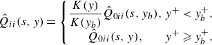 \begin{equation} {\hat {Q}}_{ii}(s,y)=\left \{\begin{matrix}\dfrac {K(y)}{K(y_{b})}{\hat {Q}}_{0ii}(s,y_b),&y^+\lt y_b^+,\\{\hat {Q}}_{0ii}(s,y),&y^+\geqslant y_b^+,\\\end{matrix}\right . \end{equation}
where ${\hat {Q}}_{0ii}(s,y)$
is the original value given by (3.6), and
${\hat {Q}}_{0ii}(s,y)$
is the original value given by (3.6), and $y_b^+=10$
.
$y_b^+=10$
.
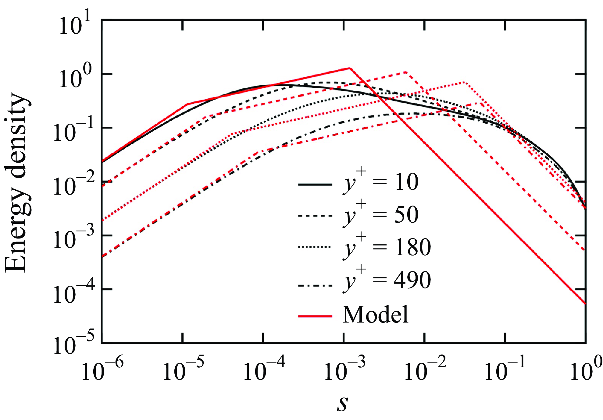
Figure 8. Profiles of pre-multiplied energy density ${s\hat {Q}}_{ii}(s,y)$
obtained from the DNS of turbulent channel flow at
${s\hat {Q}}_{ii}(s,y)$
obtained from the DNS of turbulent channel flow at ${Re}_\tau =590$
as a function of
${Re}_\tau =590$
as a function of $s$
for different
$s$
for different $y^+$
locations. The black lines denote DNS values, and the red lines denote those obtained from the model expression given by (3.6).
$y^+$
locations. The black lines denote DNS values, and the red lines denote those obtained from the model expression given by (3.6).
3.3. Non-local eddy diffusivity obtained from the model
Using the improved model in § 3.2, we evaluate the profiles of non-local eddy diffusivity in turbulent channel flow and compare them with those directly obtained from the DNS shown in § 2.3. First, we examine the one-dimensional profiles of non-local eddy diffusivity as functions of $y$
or
$y$
or $y^\prime$
. Figure 9(a) shows the profiles of
$y^\prime$
. Figure 9(a) shows the profiles of $\kappa _{NLyy}(y,y^\prime )$
as a function of
$\kappa _{NLyy}(y,y^\prime )$
as a function of $y$
for four locations of
$y$
for four locations of $y^\prime$
. The black lines represent the DNS values in figure 2(a), and the red lines represent those obtained from the model. The red line for each
$y^\prime$
. The black lines represent the DNS values in figure 2(a), and the red lines represent those obtained from the model. The red line for each $y^\prime$
location almost agrees with the corresponding DNS value, although the peak value at
$y^\prime$
location almost agrees with the corresponding DNS value, although the peak value at $y=y^\prime$
is slightly overpredicted. The asymmetry of the profiles near the wall is reproduced using the model incorporating the wall effect. Figure 9(b) shows the profiles of
$y=y^\prime$
is slightly overpredicted. The asymmetry of the profiles near the wall is reproduced using the model incorporating the wall effect. Figure 9(b) shows the profiles of $\kappa _{NLyy}(y,y^\prime )$
as a function of
$\kappa _{NLyy}(y,y^\prime )$
as a function of $y^\prime$
for four locations of
$y^\prime$
for four locations of $y$
. The agreement between the DNS and model is similar to that in figure 9(a).
$y$
. The agreement between the DNS and model is similar to that in figure 9(a).
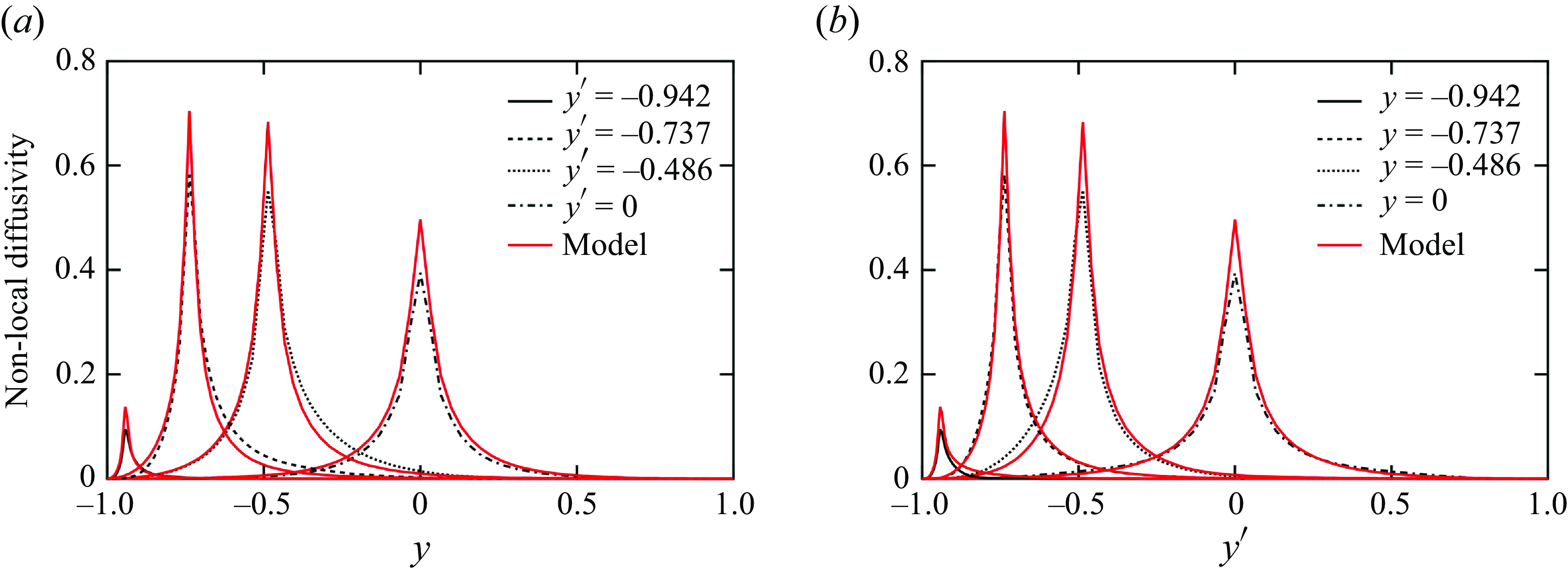
Figure 9. Profiles of non-local eddy diffusivity: (a) $\kappa _{NLyy}(y,y^\prime )$
as a function of
$\kappa _{NLyy}(y,y^\prime )$
as a function of $y$
and (b)
$y$
and (b) $\kappa _{NLyy}(y,y^\prime )$
as a function of
$\kappa _{NLyy}(y,y^\prime )$
as a function of $y^\prime$
. The black lines denote DNS values, and the red lines denote those obtained from the model.
$y^\prime$
. The black lines denote DNS values, and the red lines denote those obtained from the model.
Next, we examine the two-dimensional profiles of non-local eddy diffusivity in the streamwise and wall-normal directions. Figure 10(a) shows the two-dimensional contour plots of $\kappa _{NLyy}(x-x^\prime ,y,y^\prime )$
obtained from the model in the
$\kappa _{NLyy}(x-x^\prime ,y,y^\prime )$
obtained from the model in the $x-x^\prime$
and
$x-x^\prime$
and $y$
plane for
$y$
plane for $y^\prime =-0.737$
(
$y^\prime =-0.737$
( $y^{\prime +}=47.3$
). The profile spreading downstream shown in figure 10(a) agrees well with the DNS values shown in figure 4(a). The streamwise lengths of the contours are nearly equal in the two figures. The width of the contours in the
$y^{\prime +}=47.3$
). The profile spreading downstream shown in figure 10(a) agrees well with the DNS values shown in figure 4(a). The streamwise lengths of the contours are nearly equal in the two figures. The width of the contours in the $y$
direction in figure 10(a) is slightly smaller than that in figure 4(a). The profiles of
$y$
direction in figure 10(a) is slightly smaller than that in figure 4(a). The profiles of $\kappa _{NLyy}(x-x^\prime ,y,y^\prime )$
in the
$\kappa _{NLyy}(x-x^\prime ,y,y^\prime )$
in the $x^\prime -x$
and
$x^\prime -x$
and $y^\prime$
plane in figure 10(b) are similar to the DNS values in figure 4(b). The model reproduces the behaviour of non-local eddy diffusivity in which the mean scalar gradient in a wide upstream region significantly affects the scalar flux at a point. Figures 11(a) and 11(b) show the two-dimensional contour plots of
$y^\prime$
plane in figure 10(b) are similar to the DNS values in figure 4(b). The model reproduces the behaviour of non-local eddy diffusivity in which the mean scalar gradient in a wide upstream region significantly affects the scalar flux at a point. Figures 11(a) and 11(b) show the two-dimensional contour plots of $\kappa _{NLyy}(x-x^\prime ,y,y^\prime )$
obtained from the model for
$\kappa _{NLyy}(x-x^\prime ,y,y^\prime )$
obtained from the model for $y^\prime =-0.942$
(
$y^\prime =-0.942$
( $y^{\prime +}=10.5$
) and for
$y^{\prime +}=10.5$
) and for $y=-0.942$
(
$y=-0.942$
( $y^+=10.5$
), respectively. These profiles are similar to the DNS values shown in figure 5. The contours near the wall become almost horizontal because of the wall effect. The streamwise length of the contours in figures 11(a) and 11(b) is slightly larger than that in figures 5(a) and 5(b), but the tendency in which the length is larger in figure 5(b) than in figure 5(a) is reproduced by the model in figures 11(a) and 11(b).
$y^+=10.5$
), respectively. These profiles are similar to the DNS values shown in figure 5. The contours near the wall become almost horizontal because of the wall effect. The streamwise length of the contours in figures 11(a) and 11(b) is slightly larger than that in figures 5(a) and 5(b), but the tendency in which the length is larger in figure 5(b) than in figure 5(a) is reproduced by the model in figures 11(a) and 11(b).
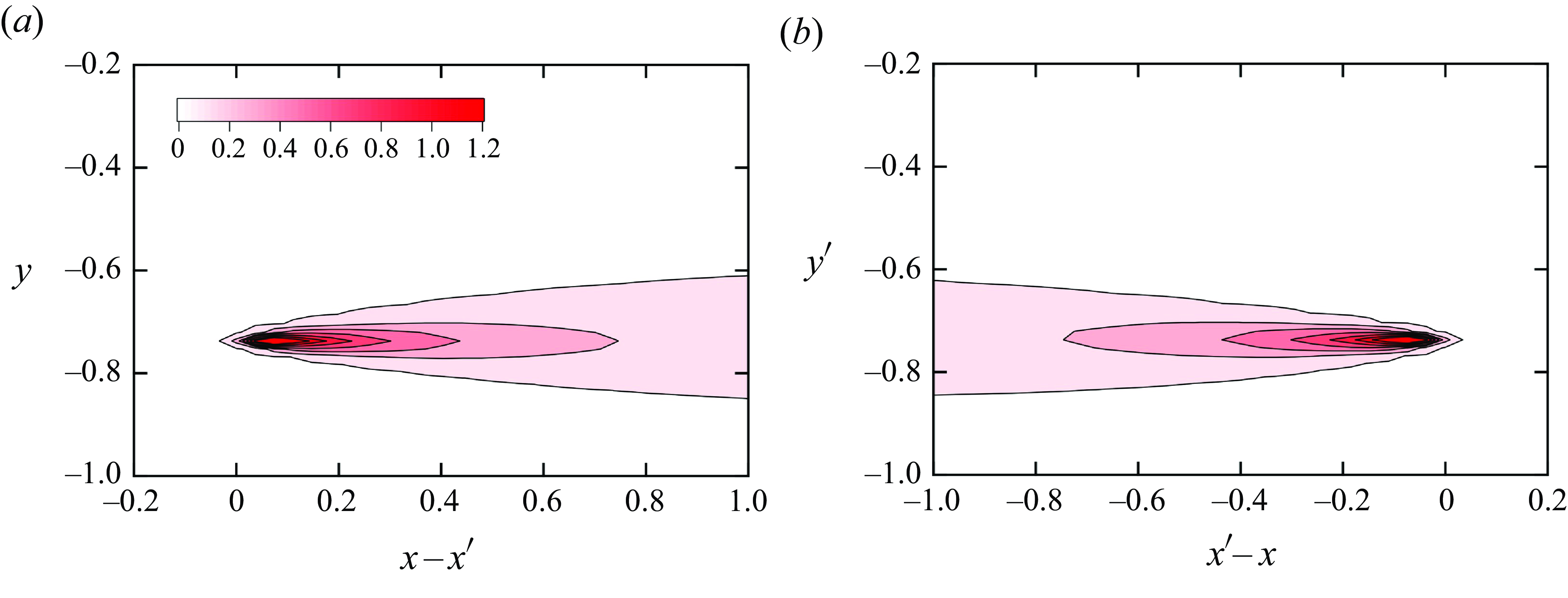
Figure 10. Contour plots of non-local eddy diffusivity obtained from the model: (a) $\kappa _{NLyy}(x-x^\prime ,y,y^\prime )$
as a function of
$\kappa _{NLyy}(x-x^\prime ,y,y^\prime )$
as a function of $x-x^\prime$
and
$x-x^\prime$
and $y$
for
$y$
for $y^\prime =-0.737$
(
$y^\prime =-0.737$
( $y^{\prime +}=47.3$
) and (b)
$y^{\prime +}=47.3$
) and (b) $\kappa _{NLyy}(x-x^\prime ,y,y^\prime )$
as a function of
$\kappa _{NLyy}(x-x^\prime ,y,y^\prime )$
as a function of $x^\prime -x$
and
$x^\prime -x$
and $y^\prime$
for
$y^\prime$
for $y=-0.737$
(
$y=-0.737$
( $y^+=47.3$
).
$y^+=47.3$
).
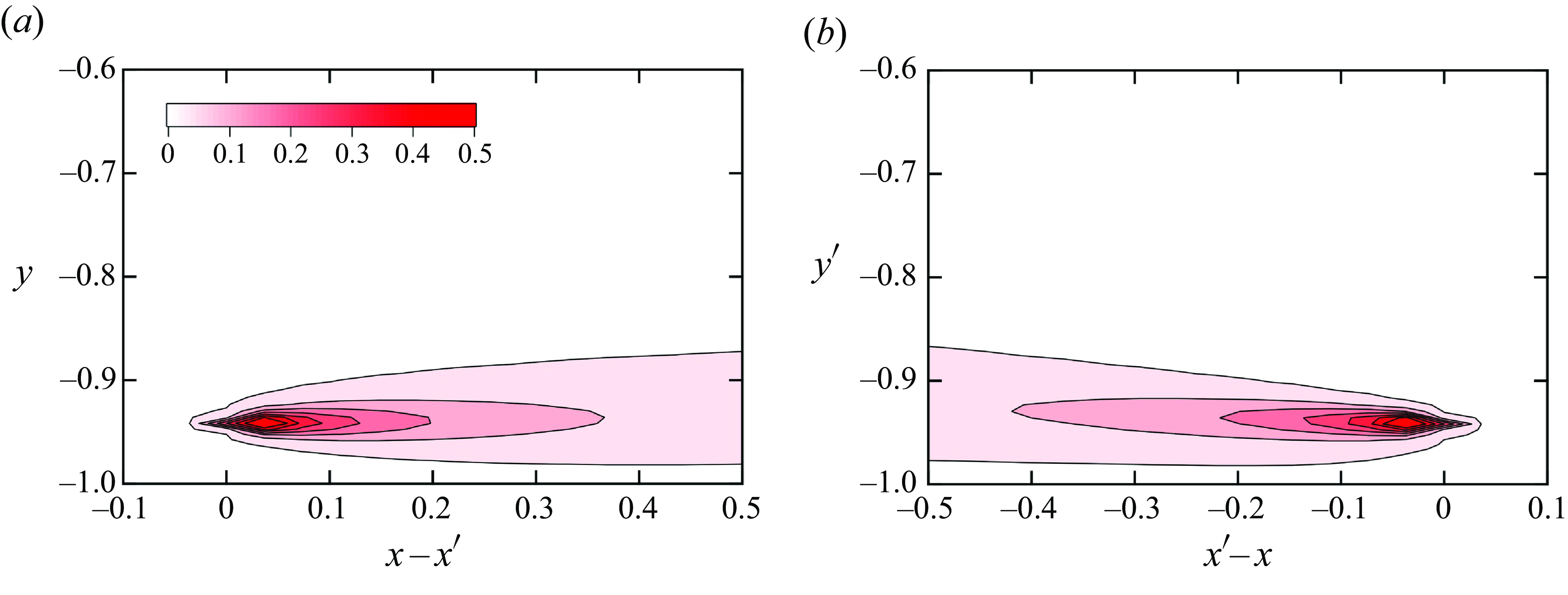
Figure 11. Contour plots of non-local eddy diffusivity obtained from the model: (a) $\kappa _{NLyy}(x-x^\prime ,y,y^\prime )$
as a function of
$\kappa _{NLyy}(x-x^\prime ,y,y^\prime )$
as a function of $x-x^\prime$
and
$x-x^\prime$
and $y$
for
$y$
for $y^\prime =-0.942$
(
$y^\prime =-0.942$
( $y^{\prime +}=10.5$
) and (b)
$y^{\prime +}=10.5$
) and (b) $\kappa _{NLyy}(x-x^\prime ,y,y^\prime )$
as a function of
$\kappa _{NLyy}(x-x^\prime ,y,y^\prime )$
as a function of $x^\prime -x$
and
$x^\prime -x$
and $y^\prime$
for
$y^\prime$
for $y=-0.942$
(
$y=-0.942$
( $y^+=10.5$
).
$y^+=10.5$
).
Figures 12(a)–12(c) show the two-dimensional contour plots of $\kappa _{NLyy}(x-x^\prime ,y,y^\prime ,\tau )$
obtained from the model in the
$\kappa _{NLyy}(x-x^\prime ,y,y^\prime ,\tau )$
obtained from the model in the $x-x^\prime$
and
$x-x^\prime$
and $y$
plane for
$y$
plane for $y^\prime =-0.737$
(
$y^\prime =-0.737$
( $y^{\prime +}=47.3$
) for the three values of
$y^{\prime +}=47.3$
) for the three values of $\tau$
. The forward diffusion profiles clearly demonstrate the role of the model expressions. The wall effect expressed in (3.19) and (3.20) is not significant because location
$\tau$
. The forward diffusion profiles clearly demonstrate the role of the model expressions. The wall effect expressed in (3.19) and (3.20) is not significant because location $y^\prime =-0.737$
is away from the wall. Note that the convection velocity
$y^\prime =-0.737$
is away from the wall. Note that the convection velocity $U_x(y^\prime )$
for
$U_x(y^\prime )$
for $r_x=x-x^\prime -U_x(y^\prime )\tau$
, the energy dissipation
$r_x=x-x^\prime -U_x(y^\prime )\tau$
, the energy dissipation $\varepsilon (y^\prime )$
appearing in (3.6) and the Reynolds stress
$\varepsilon (y^\prime )$
appearing in (3.6) and the Reynolds stress $R_{ij}(y^\prime )$
appearing in (3.15)–(3.18) are all evaluated at a single
$R_{ij}(y^\prime )$
appearing in (3.15)–(3.18) are all evaluated at a single $y^\prime$
location where the mean scalar gradient is considered; these values are fixed and independent of
$y^\prime$
location where the mean scalar gradient is considered; these values are fixed and independent of $y$
and
$y$
and $\tau$
. For a fixed value of
$\tau$
. For a fixed value of $y^\prime$
, the isosurface of
$y^\prime$
, the isosurface of $Q_{yy} (r_x,r_y,r_z,y^\prime )$
given by (3.15) with (3.4)–(3.6) as a function of
$Q_{yy} (r_x,r_y,r_z,y^\prime )$
given by (3.15) with (3.4)–(3.6) as a function of $\mathbf{r}$
becomes a sphere. The isosurface of
$\mathbf{r}$
becomes a sphere. The isosurface of $G (r_x,r_y,r_z,\tau ,y^\prime )$
given by (3.16) becomes an ellipsoid because of the anisotropic Reynolds stress
$G (r_x,r_y,r_z,\tau ,y^\prime )$
given by (3.16) becomes an ellipsoid because of the anisotropic Reynolds stress $R_{ij}(y^\prime )$
. Therefore, the two-dimensional profiles obtained from the model in figures 12(a)–12(c) become ellipses; they are elongated in the streamwise direction because
$R_{ij}(y^\prime )$
. Therefore, the two-dimensional profiles obtained from the model in figures 12(a)–12(c) become ellipses; they are elongated in the streamwise direction because $R_{xx} \gt R_{yy}$
and tilted towards the bottom wall because
$R_{xx} \gt R_{yy}$
and tilted towards the bottom wall because $R_{xy} \lt 0$
. As
$R_{xy} \lt 0$
. As $\tau$
increases, the profile moves downstream with a uniform velocity
$\tau$
increases, the profile moves downstream with a uniform velocity $U_x(y^\prime )$
, the peak value decreases and the size increases according to (3.16). This behaviour agrees with the DNS values shown in figures 6(a)–6(c) although the peak values are slightly overpredicted. Therefore, the anisotropic turbulent diffusion due to the Reynolds stress given by (3.16) can account for the behaviour of non-local eddy diffusivity shown in figures 6(a)–6(c). In contrast, figures 12(d)–12(f) show the two-dimensional contour plots of
$U_x(y^\prime )$
, the peak value decreases and the size increases according to (3.16). This behaviour agrees with the DNS values shown in figures 6(a)–6(c) although the peak values are slightly overpredicted. Therefore, the anisotropic turbulent diffusion due to the Reynolds stress given by (3.16) can account for the behaviour of non-local eddy diffusivity shown in figures 6(a)–6(c). In contrast, figures 12(d)–12(f) show the two-dimensional contour plots of $\kappa _{NLyy}(x-x^\prime ,y,y^\prime ,\tau )$
obtained from the model in the
$\kappa _{NLyy}(x-x^\prime ,y,y^\prime ,\tau )$
obtained from the model in the $x^\prime -x$
and
$x^\prime -x$
and $y^\prime$
plane for
$y^\prime$
plane for $y=-0.737$
(
$y=-0.737$
( $y^+=47.3$
). The overall profile is similar to the corresponding profile in figures 12(a)–12(c). The profiles are ellipses elongated in the streamwise direction and tilted towards the centre of the channel. As
$y^+=47.3$
). The overall profile is similar to the corresponding profile in figures 12(a)–12(c). The profiles are ellipses elongated in the streamwise direction and tilted towards the centre of the channel. As $\tau$
increases, the profile moves upstream with
$\tau$
increases, the profile moves upstream with $U_x(y^\prime )$
, the peak value decreases and the size increases. However, the profile is not a simple ellipse but is elongated asymmetrically, as shown in figures 12(d)–12(f). This asymmetric elongation is caused by the inhomogeneity effect. For example, because the convection velocity
$U_x(y^\prime )$
, the peak value decreases and the size increases. However, the profile is not a simple ellipse but is elongated asymmetrically, as shown in figures 12(d)–12(f). This asymmetric elongation is caused by the inhomogeneity effect. For example, because the convection velocity $U_x(y^\prime )$
depends on
$U_x(y^\prime )$
depends on $y^\prime$
, each part of the profile moves upstream at a different speed, that is, the mean shear elongates the profile. The dependence of
$y^\prime$
, each part of the profile moves upstream at a different speed, that is, the mean shear elongates the profile. The dependence of $R_{ij}(y^\prime )$
and
$R_{ij}(y^\prime )$
and $\varepsilon (y^\prime )$
on
$\varepsilon (y^\prime )$
on $y^\prime$
can also affect the asymmetric elongation. Therefore, elongated profiles obtained from the DNS in figure 6(d)–6(f) can be understood as the inhomogeneity effect.
$y^\prime$
can also affect the asymmetric elongation. Therefore, elongated profiles obtained from the DNS in figure 6(d)–6(f) can be understood as the inhomogeneity effect.

Figure 12. Contour plots of non-local eddy diffusivity obtained from the model: $\kappa _{NLyy}(x-x^\prime ,y,y^\prime ,\tau )$
as a function of
$\kappa _{NLyy}(x-x^\prime ,y,y^\prime ,\tau )$
as a function of $x-x^\prime$
and
$x-x^\prime$
and $y$
for
$y$
for $y^\prime =-0.737$
(
$y^\prime =-0.737$
( $y^{\prime +}=47.3$
) at (a)
$y^{\prime +}=47.3$
) at (a) $\tau =0.0225$
, (b)
$\tau =0.0225$
, (b) $\tau =0.045$
and (c)
$\tau =0.045$
and (c) $\tau =0.0675$
and
$\tau =0.0675$
and $\kappa _{NLyy}(x-x^\prime ,y,y^\prime ,\tau )$
as a function of
$\kappa _{NLyy}(x-x^\prime ,y,y^\prime ,\tau )$
as a function of $x^\prime -x$
and
$x^\prime -x$
and $y^\prime$
for
$y^\prime$
for $y=-0.737$
(
$y=-0.737$
( $y^+=47.3$
) at (d)
$y^+=47.3$
) at (d) $\tau =0.0225$
, (e)
$\tau =0.0225$
, (e) $\tau =0.045$
and (f)
$\tau =0.045$
and (f) $\tau =0.0675$
.
$\tau =0.0675$
.
Figures 13(a)–13(c) show the two-dimensional contour plots of $\kappa _{NLyy}(x-x^\prime ,y,y^\prime ,\tau )$
obtained from the model in the
$\kappa _{NLyy}(x-x^\prime ,y,y^\prime ,\tau )$
obtained from the model in the $x-x^\prime$
and
$x-x^\prime$
and $y$
plane for
$y$
plane for $y^\prime =-0.942$
(
$y^\prime =-0.942$
( $y^{\prime +}=10.5$
) for the three values of
$y^{\prime +}=10.5$
) for the three values of $\tau$
. The behaviour of the contours moving downstream is similar to that shown in figures 12(a)–12(c). Because the
$\tau$
. The behaviour of the contours moving downstream is similar to that shown in figures 12(a)–12(c). Because the $y^\prime$
location is close to the bottom wall, the convection velocity
$y^\prime$
location is close to the bottom wall, the convection velocity $U_x(y^\prime )$
is low and the contours are nearly horizontal owing to the wall effect. This behaviour agrees with the DNS values shown in figures 7(a)–7(c), although the peak values are overpredicted and the width of the contours in the wall-normal direction is slightly underpredicted. Figures 13(d)–13(f) show the two-dimensional contour plots of
$U_x(y^\prime )$
is low and the contours are nearly horizontal owing to the wall effect. This behaviour agrees with the DNS values shown in figures 7(a)–7(c), although the peak values are overpredicted and the width of the contours in the wall-normal direction is slightly underpredicted. Figures 13(d)–13(f) show the two-dimensional contour plots of $\kappa _{NLyy}(x-x^\prime ,y,y^\prime ,\tau )$
obtained from the model in the
$\kappa _{NLyy}(x-x^\prime ,y,y^\prime ,\tau )$
obtained from the model in the $x^\prime -x$
and
$x^\prime -x$
and $y^\prime$
plane for
$y^\prime$
plane for $y=-0.942$
(
$y=-0.942$
( $y^+=10.5$
). The asymmetric elongation of the profiles is clearly shown in figures 13(e) and 13(f). The profile shown in figure 13(f) is much longer in the streamwise direction than that shown in figure 13(c). This significant elongation is caused by the strong mean shear of
$y^+=10.5$
). The asymmetric elongation of the profiles is clearly shown in figures 13(e) and 13(f). The profile shown in figure 13(f) is much longer in the streamwise direction than that shown in figure 13(c). This significant elongation is caused by the strong mean shear of $U_x(y^\prime )$
near the wall. The same behaviour is observed for the DNS values shown in figures 7(c) and 7(f). Therefore, the improved model reasonably reproduces the temporal behaviour of non-local eddy diffusivity obtained from the DNS.
$U_x(y^\prime )$
near the wall. The same behaviour is observed for the DNS values shown in figures 7(c) and 7(f). Therefore, the improved model reasonably reproduces the temporal behaviour of non-local eddy diffusivity obtained from the DNS.
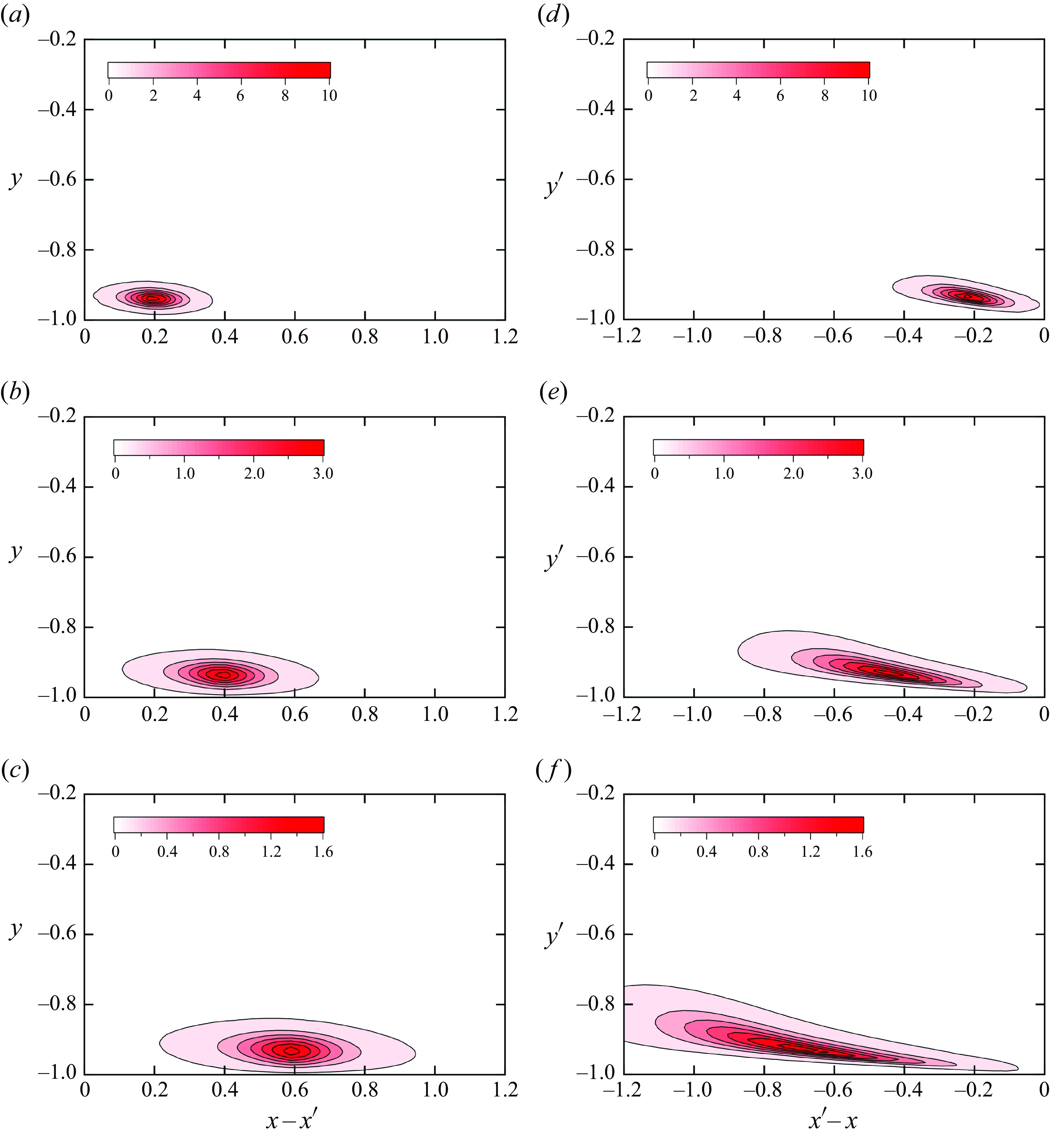
Figure 13. Contour plots of non-local eddy diffusivity obtained from the model: $\kappa _{NLyy}(x-x^\prime ,y,y^\prime ,\tau )$
as a function of
$\kappa _{NLyy}(x-x^\prime ,y,y^\prime ,\tau )$
as a function of $x-x^\prime$
and
$x-x^\prime$
and $y$
for
$y$
for $y^\prime =-0.942$
(
$y^\prime =-0.942$
( $y^{\prime +}=10.5$
) at (a)
$y^{\prime +}=10.5$
) at (a) $\tau =0.0225$
, (b)
$\tau =0.0225$
, (b) $\tau =0.045$
and (c)
$\tau =0.045$
and (c) $\tau =0.0675$
and
$\tau =0.0675$
and $\kappa _{NLyy}(x-x^\prime ,y,y^\prime ,\tau )$
as a function of
$\kappa _{NLyy}(x-x^\prime ,y,y^\prime ,\tau )$
as a function of $x^\prime -x$
and
$x^\prime -x$
and $y^\prime$
for
$y^\prime$
for $y=-0.942$
(
$y=-0.942$
( $y^+=10.5$
) at (d)
$y^+=10.5$
) at (d) $\tau =0.0225$
, (e)
$\tau =0.0225$
, (e) $\tau =0.045$
and (f)
$\tau =0.045$
and (f) $\tau =0.0675$
.
$\tau =0.0675$
.
Here, we mention the dependence of the model expression on the $y^\prime$
location. Based on the model expression for homogeneous isotropic turbulence described in § 3.1, we incorporate the inhomogeneity effect into the model in § 3.2. In this procedure, whether statistical quantities should depend on
$y^\prime$
location. Based on the model expression for homogeneous isotropic turbulence described in § 3.1, we incorporate the inhomogeneity effect into the model in § 3.2. In this procedure, whether statistical quantities should depend on $y$
or on
$y$
or on $y^\prime$
is not trivial. In the present model, quantities such as
$y^\prime$
is not trivial. In the present model, quantities such as $U_x(y^\prime )$
and
$U_x(y^\prime )$
and $R_{ij}(y^\prime )$
are assumed to be functions of
$R_{ij}(y^\prime )$
are assumed to be functions of $y^\prime$
. Other choices for the
$y^\prime$
. Other choices for the $y$
and
$y$
and $y^\prime$
dependence of the model are possible, such as
$y^\prime$
dependence of the model are possible, such as $U_x(y)$
and
$U_x(y)$
and $U_x((y+y^\prime )/2)$
, but resulting profiles of non-local eddy diffusivity must be different from figures 12 and 13. Because the present model approximately reproduced the DNS results shown in figures 6 and 7, we consider the
$U_x((y+y^\prime )/2)$
, but resulting profiles of non-local eddy diffusivity must be different from figures 12 and 13. Because the present model approximately reproduced the DNS results shown in figures 6 and 7, we consider the $y^\prime$
dependence of the present model to be adequate.
$y^\prime$
dependence of the present model to be adequate.
Using this model, we can understand the behaviour of non-local eddy diffusivity as follows. The forward diffusion process shown in figures 12(a)–12(c) and 13(a)–13(c) is rather simple: as $\tau$
increases, a profile moves downstream with a uniform velocity
$\tau$
increases, a profile moves downstream with a uniform velocity $U_x(y^\prime )$
and diffuses anisotropically owing to a fixed value of
$U_x(y^\prime )$
and diffuses anisotropically owing to a fixed value of $R_{ij}(y^\prime )$
. In contrast, the backward diffusion process shown in figures 12(d)–12(f) and 13(d)–13(f) becomes rather complicated: as
$R_{ij}(y^\prime )$
. In contrast, the backward diffusion process shown in figures 12(d)–12(f) and 13(d)–13(f) becomes rather complicated: as $\tau$
increases, a profile moves upstream with a non-uniform velocity
$\tau$
increases, a profile moves upstream with a non-uniform velocity $U_x(y^\prime )$
and diffuses anisotropically owing to a non-uniform value of
$U_x(y^\prime )$
and diffuses anisotropically owing to a non-uniform value of $R_{ij}(y^\prime )$
, resulting an asymmetric elongation of the profile.
$R_{ij}(y^\prime )$
, resulting an asymmetric elongation of the profile.
Note that the two-dimensional contours shown in figures 10 and 11 are obtained by integrating the temporal profiles shown in figures 12 and 13 with respect to $\tau$
. Subsequently, one-dimensional profiles shown in figure 9 are obtained by integrating the two-dimensional profiles shown in figures 10 and 11 with respect to
$\tau$
. Subsequently, one-dimensional profiles shown in figure 9 are obtained by integrating the two-dimensional profiles shown in figures 10 and 11 with respect to $x-x^\prime$
. Therefore, the profiles in figures 9–11 can be understood as the accumulated effects of mean flow convection and anisotropic turbulent diffusion shown in figures 12 and 13.
$x-x^\prime$
. Therefore, the profiles in figures 9–11 can be understood as the accumulated effects of mean flow convection and anisotropic turbulent diffusion shown in figures 12 and 13.
Figures 10(b), 11(b), 12(f) and 13(f) suggest that the mean scalar gradient in a wide upstream region significantly affects the scalar flux at a downstream point. Such a non-local property is important in scalar diffusion problems where the mean scalar profile is inhomogeneous in the streamwise direction, unlike the present channel flow. An example is the diffusion of a chemically reactive species released from a factory. The profile of the mean scalar changes rapidly near the point source, and the length scale of the mean scalar can be much smaller than the scale of velocity fluctuations in the atmospheric boundary layer. In this case, simulation results with local models are expected to be inaccurate, and non-local models must be used to accurately predict the scalar flux in the downstream region.
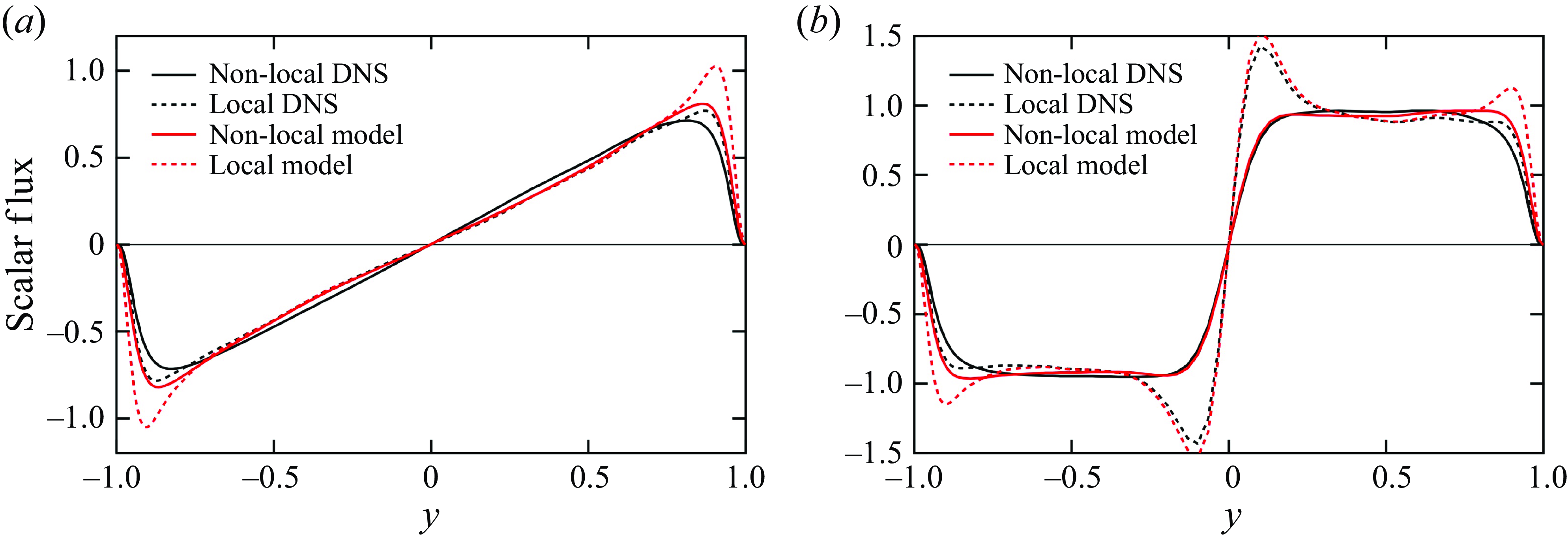
Figure 14. Profiles of the scalar fluxes $\langle u_y\theta \rangle _{NL}$
and
$\langle u_y\theta \rangle _{NL}$
and $\langle u_y\theta \rangle _{L}$
obtained from the DNS and the model as functions of
$\langle u_y\theta \rangle _{L}$
obtained from the DNS and the model as functions of $y$
for (a) case 1 and (b) case 2. ‘Non-local DNS’ denotes
$y$
for (a) case 1 and (b) case 2. ‘Non-local DNS’ denotes $\langle u_y\theta \rangle _{NL}$
with DNS data, ‘Local DNS’ denotes
$\langle u_y\theta \rangle _{NL}$
with DNS data, ‘Local DNS’ denotes $\langle u_y\theta \rangle _{L}$
with DNS data, ‘Non-local model’ denotes
$\langle u_y\theta \rangle _{L}$
with DNS data, ‘Non-local model’ denotes $\langle u_y\theta \rangle _{NL}$
with the model and ‘Local model’ denotes
$\langle u_y\theta \rangle _{NL}$
with the model and ‘Local model’ denotes $\langle u_y\theta \rangle _{L}$
with the model.
$\langle u_y\theta \rangle _{L}$
with the model.
3.4. Turbulent scalar flux obtained from the model
The one-dimensional profiles of non-local eddy diffusivity obtained from the model are shown in figure 9. Here, we examine how turbulent scalar flux is evaluated using the non-local eddy diffusivity model. Figure 14 shows the profiles of the scalar fluxes $\langle u_y\theta \rangle _{NL}$
and
$\langle u_y\theta \rangle _{NL}$
and $\langle u_y\theta \rangle _{L}$
obtained from the DNS and model for the two cases. The black lines denote the profiles of the non-local expression
$\langle u_y\theta \rangle _{L}$
obtained from the DNS and model for the two cases. The black lines denote the profiles of the non-local expression $\langle u_y\theta \rangle _{NL}$
given by (2.12) and the local expression
$\langle u_y\theta \rangle _{NL}$
given by (2.12) and the local expression $\langle u_y\theta \rangle _{L}$
given by (2.14) and (2.15); in both expressions exact DNS values of
$\langle u_y\theta \rangle _{L}$
given by (2.14) and (2.15); in both expressions exact DNS values of $\kappa _{NLyy}(y,y^\prime )$
are used. The red lines denote the profiles of the non-local and local expressions in which the values of the model of
$\kappa _{NLyy}(y,y^\prime )$
are used. The red lines denote the profiles of the non-local and local expressions in which the values of the model of $\kappa _{NLyy}(y,y^\prime )$
are used. At
$\kappa _{NLyy}(y,y^\prime )$
are used. At $-0.8\lt y\lt 0.8$
, the non-local model, plotted as a red solid line, almost agrees well with the DNS value, plotted as a black solid line, in both cases. In particular, in figure 14(b) for case 2, the non-local model predicts the scalar flux accurately within
$-0.8\lt y\lt 0.8$
, the non-local model, plotted as a red solid line, almost agrees well with the DNS value, plotted as a black solid line, in both cases. In particular, in figure 14(b) for case 2, the non-local model predicts the scalar flux accurately within $-0.25\lt y\lt 0.25$
where the local expression overpredicts it significantly. In contrast, near the wall within
$-0.25\lt y\lt 0.25$
where the local expression overpredicts it significantly. In contrast, near the wall within $-1\lt y\lt -0.8$
and
$-1\lt y\lt -0.8$
and $0.8\lt y\lt 1$
the non-local model slightly overpredicts the DNS value in both cases. These results suggest that the non-local eddy diffusivity model described in § 3.2 still requires improvement near the wall.
$0.8\lt y\lt 1$
the non-local model slightly overpredicts the DNS value in both cases. These results suggest that the non-local eddy diffusivity model described in § 3.2 still requires improvement near the wall.
Figure 15. Profiles of the scalar fluxes $\langle u_y\theta \rangle _{NL}$
and
$\langle u_y\theta \rangle _{NL}$
and $\langle u_y\theta \rangle _{L}$
obtained from the DNS and the modified model as functions of
$\langle u_y\theta \rangle _{L}$
obtained from the DNS and the modified model as functions of $y$
for case 1. ‘Non-local DNS’ denotes
$y$
for case 1. ‘Non-local DNS’ denotes $\langle u_y\theta \rangle _{NL}$
with DNS data, ‘Local DNS’ denotes
$\langle u_y\theta \rangle _{NL}$
with DNS data, ‘Local DNS’ denotes $\langle u_y\theta \rangle _{L}$
with DNS data, ‘Non-local model’ denotes
$\langle u_y\theta \rangle _{L}$
with DNS data, ‘Non-local model’ denotes $\langle u_y\theta \rangle _{NL}$
with the model and ‘Local model’ denotes
$\langle u_y\theta \rangle _{NL}$
with the model and ‘Local model’ denotes $\langle u_y\theta \rangle _{L}$
with the model.
$\langle u_y\theta \rangle _{L}$
with the model.
One of the reasons for this overprediction is the inaccurate modelling of ${\hat {Q}}_{ii}(s,y)$
near the wall, as shown in figure 8. Here, we attempt to improve the expression for
${\hat {Q}}_{ii}(s,y)$
near the wall, as shown in figure 8. Here, we attempt to improve the expression for ${\hat {Q}}_{ii}(s,y)$
near a wall. In (3.20), where the method of images is used, the following factor is used:
${\hat {Q}}_{ii}(s,y)$
near a wall. In (3.20), where the method of images is used, the following factor is used:
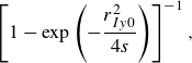 \begin{equation} \left [1-\exp \left (-\frac {r_{Iy0}^2}{4s}\right )\right ]^{-1} , \end{equation}
where $r_{Iy0}[=2(1+y)]=2y_w$
and
$r_{Iy0}[=2(1+y)]=2y_w$
and $y_w$
is the distance from the wall. Because the factor tends to unity when
$y_w$
is the distance from the wall. Because the factor tends to unity when $y_w$
is sufficiently large, it does not change the integrand in (3.20) away from the wall. This behaviour suggests that
$y_w$
is sufficiently large, it does not change the integrand in (3.20) away from the wall. This behaviour suggests that $y_w^2/s$
can be an important quantity related to the wall effect which vanishes away from the wall. Using this quantity, we empirically model the energy density as
$y_w^2/s$
can be an important quantity related to the wall effect which vanishes away from the wall. Using this quantity, we empirically model the energy density as
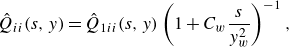 \begin{equation} {\hat {Q}}_{ii}(s,y)={\hat {Q}}_{1ii}(s,y)\left (1+C_w\frac {s}{y_w^2}\right )^{-1} , \end{equation}
where ${\hat {Q}}_{1ii}(s,y)$
is the energy density given by (3.22), and
${\hat {Q}}_{1ii}(s,y)$
is the energy density given by (3.22), and $C_w=0.1$
. For a fixed value of
$C_w=0.1$
. For a fixed value of $s$
, the correction factor
$s$
, the correction factor $(1+C_ws/y_w^2)^{-1}$
decreases to a small value near the wall and tends to unity away from the wall, where
$(1+C_ws/y_w^2)^{-1}$
decreases to a small value near the wall and tends to unity away from the wall, where $y_w$
is sufficiently large.
$y_w$
is sufficiently large.
Figure 15 shows the profiles of the scalar fluxes $\langle u_y\theta \rangle _{NL}$
and
$\langle u_y\theta \rangle _{NL}$
and $\langle u_y\theta \rangle _{L}$
obtained from the DNS and modified model for case 1. The non-local model, plotted as a red solid line, agrees with the DNS value, plotted as a black solid line, near the wall. Although the modification given by (3.24) has not yet been physically justified, this agreement suggests that the accurate modelling of
$\langle u_y\theta \rangle _{L}$
obtained from the DNS and modified model for case 1. The non-local model, plotted as a red solid line, agrees with the DNS value, plotted as a black solid line, near the wall. Although the modification given by (3.24) has not yet been physically justified, this agreement suggests that the accurate modelling of ${\hat {Q}}_{ii}(s,y)$
near the wall can improve the performance of the non-local eddy diffusivity model. In future studies, we will examine the profile of
${\hat {Q}}_{ii}(s,y)$
near the wall can improve the performance of the non-local eddy diffusivity model. In future studies, we will examine the profile of ${\hat {Q}}_{ii}(s,y)$
in detail and propose a model based on physical mechanisms.
${\hat {Q}}_{ii}(s,y)$
in detail and propose a model based on physical mechanisms.
The proposed model for $\kappa _{NLyy}(x-x^\prime ,y,y^\prime ,z-z^\prime ,\tau )$
consists of (3.6), (3.14), (3.15), (3.19) and (3.20). The needed inputs from the flow to evaluate the model are the Reynolds stress
$\kappa _{NLyy}(x-x^\prime ,y,y^\prime ,z-z^\prime ,\tau )$
consists of (3.6), (3.14), (3.15), (3.19) and (3.20). The needed inputs from the flow to evaluate the model are the Reynolds stress $R_{ij}(y)$
and the dissipation rate
$R_{ij}(y)$
and the dissipation rate $\varepsilon (y)$
. No information of two-point correlations is needed. Nevertheless, the model expressions are too complex for a practical turbulence model. Here, we discuss a possible simplification of the present model. The expression for the correlation
$\varepsilon (y)$
. No information of two-point correlations is needed. Nevertheless, the model expressions are too complex for a practical turbulence model. Here, we discuss a possible simplification of the present model. The expression for the correlation $Q_{ii}(r)$
given by (3.4), (3.5) and (3.6) is based on the velocity fluctuations from small to large scales. It can be simplified by focusing only on large scales as follows:
$Q_{ii}(r)$
given by (3.4), (3.5) and (3.6) is based on the velocity fluctuations from small to large scales. It can be simplified by focusing only on large scales as follows:
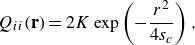 \begin{equation} Q_{ii}(\mathbf{r})=2K\exp \left (-\frac {r^2}{4s_c}\right ) , \end{equation}
where $s_{c}$
is the scale in the energy-containing range. For homogeneous isotropic turbulence, the non-local eddy diffusivity
$s_{c}$
is the scale in the energy-containing range. For homogeneous isotropic turbulence, the non-local eddy diffusivity $\kappa _{NL}(r,\tau )$
can be written as
$\kappa _{NL}(r,\tau )$
can be written as
 \begin{equation} \kappa _{NL}(r,\tau )=\frac {1}{3}G(r,\tau )Q_{ii}(\mathbf{r})=\frac {2K}{3(4\pi )^{3/2}(C_{\omega G}u_0\tau )^3}\exp \left \{-\left [\frac {1}{4(C_{\omega G}u_0\tau )^2}+\frac {1}{4s_c}\right ]r^2\right \} . \end{equation}
Moreover, for steady turbulence, the non-local eddy diffusivity $\kappa _{NL}(r)$
is given by
$\kappa _{NL}(r)$
is given by
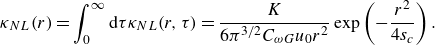 \begin{equation} \kappa _{NL}(r)=\int _{0}^{\infty }\mathrm{d}\tau \kappa _{NL}(r,\tau )=\frac {K}{6\pi ^{3/2}C_{\omega G}u_0r^2}\exp \left (-\frac {r^2}{4s_c}\right ) . \end{equation}
Using the simple expression, non-local properties can be incorporated into a model of the turbulent scalar flux. Results obtained from the simple model may be inaccurate, and some empirical factors, such as the wall damping function, may be needed to compensate for the simplification. In this case, such factors can be suggested by comparing the simple model with the present model. The proposed non-local models have not yet been applied to turbulence simulations. In future studies, such a simplified model will be applied to actual turbulence simulations. The present model is expected to be useful for proposing and improving simple practical models.
4. Conclusions
A non-local expression for the turbulent scalar flux is investigated using the DNS data of turbulent channel flow. In addition to the velocity and scalar, the Green’s function for scalar fluctuation is evaluated to obtain non-local eddy diffusivity. We have verified that the non-local expression for scalar flux agrees with the directly obtained value. In contrast, the local expression significantly overpredicts the DNS value in the region where the mean scalar gradient changes rapidly. The profile of non-local eddy diffusivity is analysed in detail using DNS data. First, one-dimensional profiles of non-local eddy diffusivity are evaluated to examine how the mean scalar gradient at a wall-normal location contributes to the scalar flux at a different location. Two-dimensional profiles of non-local eddy diffusivity in the streamwise and wall-normal directions are evaluated to examine the effects of mean flow convection and turbulent diffusion. The profiles reveal a contribution to the scalar flux from the mean scalar gradient in a wide upstream region. Additionally, we show that the temporal profile of non-local eddy diffusivity moves downstream, diffuses anisotropically and is tilted towards the wall. The profile of the backward diffusion moving upstream is elongated more significantly than that of the forward diffusion.
To better understand the behaviour of non-local eddy diffusivity and to take the first step towards improving practical turbulence models from a non-local perspective, we investigate a model expression for non-local eddy diffusivity for inhomogeneous turbulence. A model expression was proposed for homogeneous isotropic turbulence in Hamba (Reference Hamba2022 b, Reference Hamba2023). In this paper, we modify the model by incorporating the effects of turbulence anisotropy, inhomogeneity and wall boundaries. The one- and two-dimensional profiles of non-local eddy diffusivity obtained from the model agree reasonably well with the DNS values. The model reproduced the behaviour of the profiles as convection based on the mean velocity and anisotropic turbulent diffusion related to the Reynolds stress. In particular, the behaviour of backward diffusion, in which the contours are elongated more significantly than those of forward diffusion, can be understood as the inhomogeneity effect. The model accurately reproduced the turbulent scalar flux at the centre of the channel, where the mean scalar gradient changes rapidly. Because the scalar flux is slightly overpredicted near the wall, the model still requires to be improved based on physical mechanisms. Nevertheless, the results clearly indicate the potential of the non-local eddy diffusivity model. The analysis and modelling of non-local eddy diffusivity provides insights into scalar transport in inhomogeneous turbulence.
Funding
This work was supported by JSPS KAKENHI Grant number 23K03670.
Declaration of interests
The author reports no conflict of interest.
Appendix A. Green’s function for scalar fluctuation
The transport equation for the scalar fluctuation $\theta$
is given by
$\theta$
is given by
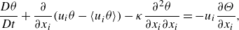 \begin{equation} \frac {D\theta }{Dt}+\frac {\partial }{\partial x_i}(u_i\theta -{\langle u}_i\theta \rangle )-\kappa \frac {\partial ^2\theta }{\partial x_i\partial x_i}=-u_i\frac {\partial \Theta }{\partial x_i} , \end{equation}
where $D/Dt=\partial /\partial t+U_i\partial /\partial x_i$
. By considering the right-hand side of (A1) as a source term for
$D/Dt=\partial /\partial t+U_i\partial /\partial x_i$
. By considering the right-hand side of (A1) as a source term for $\theta$
, we introduce the Green’s function
$\theta$
, we introduce the Green’s function $g_i(\mathbf{x},t;\mathbf{x}^\prime ,t^\prime )$
which satisfies
$g_i(\mathbf{x},t;\mathbf{x}^\prime ,t^\prime )$
which satisfies
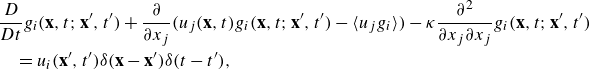 \begin{align} &\frac {D}{Dt}g_i(\mathbf{x},t;\mathbf{x}^\prime ,t^\prime )+\frac {\partial }{\partial x_j}(u_j(\mathbf{x},t)g_i(\mathbf{x},t;\mathbf{x}^\prime ,t^\prime )-\langle u_jg_i\rangle )-\kappa \frac {\partial ^2}{\partial x_j\partial x_j}g_i(\mathbf{x},t;\mathbf{x}^\prime ,t^\prime ) \nonumber \\&\quad =u_i(\mathbf{x}^\prime ,t^\prime )\delta (\mathbf{x}-\mathbf{x}^\prime )\delta (t-t^\prime ) , \end{align}
where $\delta (\mathbf{x})$
and
$\delta (\mathbf{x})$
and $\delta (t)$
are three- and one-dimensional Dirac delta functions, respectively. Note that the velocity fluctuation
$\delta (t)$
are three- and one-dimensional Dirac delta functions, respectively. Note that the velocity fluctuation $u_i(\mathbf{x}^\prime ,t^\prime )$
is included on the right-hand side of (A2). The Green’s function
$u_i(\mathbf{x}^\prime ,t^\prime )$
is included on the right-hand side of (A2). The Green’s function $g_i(\mathbf{x},t;\mathbf{x}^\prime ,t^\prime )$
represents a scalar field at
$g_i(\mathbf{x},t;\mathbf{x}^\prime ,t^\prime )$
represents a scalar field at $(\mathbf{x},t)$
associated with a point source at
$(\mathbf{x},t)$
associated with a point source at $(\mathbf{x}^\prime ,t^\prime )$
whose value is proportional to
$(\mathbf{x}^\prime ,t^\prime )$
whose value is proportional to $u_i(\mathbf{x}^\prime ,t^\prime )$
. Using the Green’s function, the formal solution to (A1) can be expressed as
$u_i(\mathbf{x}^\prime ,t^\prime )$
. Using the Green’s function, the formal solution to (A1) can be expressed as
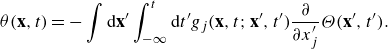 \begin{equation} \theta (\mathbf{x},t)=-\int {\mathrm{d}\mathbf{x}^\prime }\int _{-\infty }^{t}{\mathrm{d}t^\prime }g_j(\mathbf{x},t;\mathbf{x}^\prime ,t^\prime )\frac {\partial }{\partial x_j^\prime }\Theta (\mathbf{x}^\prime ,t^\prime ) . \end{equation}
By multiplying it by $u_i(\mathbf{x},t)$
and taking the ensemble averaging, we obtain the turbulent scalar flux
$u_i(\mathbf{x},t)$
and taking the ensemble averaging, we obtain the turbulent scalar flux $\langle u_i\theta \rangle$
given by (2.3) with (2.4).
$\langle u_i\theta \rangle$
given by (2.3) with (2.4).
Appendix B. Energy density and two-point velocity correlation in scale space
The two-point velocity correlation $Q_{ii}(\mathbf{r})$
used in (3.2) was expressed in terms of energy spectrum
$Q_{ii}(\mathbf{r})$
used in (3.2) was expressed in terms of energy spectrum $E(k)$
in Hamba (Reference Hamba2022b
). Because the Fourier transform of the velocity in homogeneous directions was used to define the energy spectrum, it is unclear whether the model can be applied to inhomogeneous turbulence. In Hamba (Reference Hamba2023), the model was improved using the energy density in the scale space instead of the energy spectrum in the wavenumber space. The scale-space energy density was based on filtered velocities (Hamba, Reference Hamba2022a
). The first filtered velocity
$E(k)$
in Hamba (Reference Hamba2022b
). Because the Fourier transform of the velocity in homogeneous directions was used to define the energy spectrum, it is unclear whether the model can be applied to inhomogeneous turbulence. In Hamba (Reference Hamba2023), the model was improved using the energy density in the scale space instead of the energy spectrum in the wavenumber space. The scale-space energy density was based on filtered velocities (Hamba, Reference Hamba2022a
). The first filtered velocity ${\bar {u}}_i(\mathbf{x},s)$
is defined as
${\bar {u}}_i(\mathbf{x},s)$
is defined as
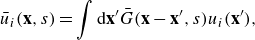 \begin{equation} {\bar {u}}_i(\mathbf{x},s)=\int {\mathrm{d}\mathbf{x}^\prime }\bar {G}(\mathbf{x}-\mathbf{x}^\prime ,s)u_i(\mathbf{x}^\prime ) , \end{equation}
where $\bar {G}(\mathbf{x},s)$
is a filter function given by
$\bar {G}(\mathbf{x},s)$
is a filter function given by
 \begin{equation} \bar {G}(\mathbf{x},s)=\frac {1}{{(2\pi s)}^{3/2}}\exp \left (-\frac {\mathbf{x}^2}{2s}\right ) . \end{equation}
Note that the quantity $s$
appearing in (B1) and (B2), which has the dimension of the square of the length, is called the scale. The filtered velocity
$s$
appearing in (B1) and (B2), which has the dimension of the square of the length, is called the scale. The filtered velocity ${\bar {u}}_i(\mathbf{x},s)$
represents the velocity with a scale equal to or greater than
${\bar {u}}_i(\mathbf{x},s)$
represents the velocity with a scale equal to or greater than $s$
.
$s$
.
By differentiating ${\bar {u}}_i(\mathbf{x},s)$
by
${\bar {u}}_i(\mathbf{x},s)$
by $s$
, we can obtain the second filtered velocity
$s$
, we can obtain the second filtered velocity ${\hat {u}}_i(\mathbf{x},s)$
given by
${\hat {u}}_i(\mathbf{x},s)$
given by
 \begin{equation} {\hat {u}}_i(\mathbf{x},s)\equiv -\frac {\partial }{\partial s}{\bar {u}}_i(\mathbf{x},s)=\int {\mathrm{d}\mathbf{x}^\prime }\hat {G}(\mathbf{x}-\mathbf{x}^\prime ,s)u_i(\mathbf{x}^\prime ) , \end{equation}
where
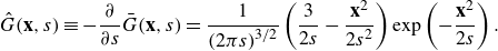 \begin{equation} \hat {G}(\mathbf{x},s)\equiv -\frac {\partial }{\partial s}\bar {G}(\mathbf{x},s)=\frac {1}{{(2\pi s)}^{3/2}}\left (\frac {3}{2s}-\frac {\mathbf{x}^2}{2s^2}\right )\exp \left (-\frac {\mathbf{x}^2}{2s}\right ) . \end{equation}
The filtered velocity ${\hat {u}}_i(\mathbf{x},s)$
represents the velocity with a scale equal to
${\hat {u}}_i(\mathbf{x},s)$
represents the velocity with a scale equal to $s$
. The original velocity
$s$
. The original velocity $u_i(\mathbf{x})$
can be expressed in terms of
$u_i(\mathbf{x})$
can be expressed in terms of ${\hat {u}}_i(\mathbf{x},s)$
as
${\hat {u}}_i(\mathbf{x},s)$
as
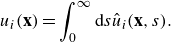 \begin{equation} u_i(\mathbf{x})=\int _{0}^{\infty }\mathrm{d}s{\hat {u}}_i(\mathbf{x},s) . \end{equation}
This equation indicates that the velocity $u_i(\mathbf{x})$
is decomposed into modes
$u_i(\mathbf{x})$
is decomposed into modes ${\hat {u}}_i(\mathbf{x},s)$
in the scale space.
${\hat {u}}_i(\mathbf{x},s)$
in the scale space.
We further consider the two-point correlation of the filtered velocities at the same scale as
 \begin{equation} {\bar {Q}}_{ii}(\mathbf{x},\mathbf{x}^\prime ,s)=\langle {\bar {u}}_i(\mathbf{x},s){\bar {u}}_i(\mathbf{x}^\prime ,s)\rangle . \end{equation}
Another correlation can be defined as
 \begin{equation} {\hat {Q}}_{ii}(\mathbf{x},\mathbf{x}^\prime ,s)\equiv -\frac {\partial }{\partial s}{\bar {Q}}_{ii}(\mathbf{x},\mathbf{x}^\prime ,s)=\langle {\hat {u}}_i(\mathbf{x},s){\bar {u}}_i(\mathbf{x}^\prime ,s)\rangle +\langle {\bar {u}}_i(\mathbf{x},s){\hat {u}}_i(\mathbf{x}^\prime ,s)\rangle . \end{equation}
Using the second correlation ${\hat {Q}}_{ii}(\mathbf{x},\mathbf{x}^\prime ,s)$
, we can decompose the original velocity correlation
${\hat {Q}}_{ii}(\mathbf{x},\mathbf{x}^\prime ,s)$
, we can decompose the original velocity correlation $Q_{ii}(\mathbf{x},\mathbf{x}^\prime )(=\langle u_i(\mathbf{x})u_i(\mathbf{x}^\prime )\rangle )$
into modes in the scale space as follows:
$Q_{ii}(\mathbf{x},\mathbf{x}^\prime )(=\langle u_i(\mathbf{x})u_i(\mathbf{x}^\prime )\rangle )$
into modes in the scale space as follows:
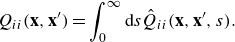 \begin{equation} Q_{ii}(\mathbf{x},\mathbf{x}^\prime )=\int _{0}^{\infty }\mathrm{d}s{\hat {Q}}_{ii}(\mathbf{x},\mathbf{x}^\prime ,s) . \end{equation}
For homogeneous turbulence, (B8) can be expressed as
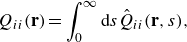 \begin{equation} Q_{ii}(\mathbf{r})=\int _{0}^{\infty }\mathrm{d}s{\hat {Q}}_{ii}(\mathbf{r},s) , \end{equation}
where $\mathbf{r}=\mathbf{x}-\mathbf{x}^\prime$
. Moreover, when
$\mathbf{r}=\mathbf{x}-\mathbf{x}^\prime$
. Moreover, when $\mathbf{r}=\mathbf{0}$
, the velocity correlation represents the turbulent kinetic energy
$\mathbf{r}=\mathbf{0}$
, the velocity correlation represents the turbulent kinetic energy $Q_{ii}(\mathbf{0})=\langle u_i^2\rangle$
, and (B9) can be expressed as
$Q_{ii}(\mathbf{0})=\langle u_i^2\rangle$
, and (B9) can be expressed as
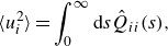 \begin{equation} \langle u_i^2\rangle =\int _{0}^{\infty }\mathrm{d}s{\hat {Q}}_{ii}(s) , \end{equation}
where ${\hat {Q}}_{ii}(s)(={\hat {Q}}_{ii}(\mathbf{0},s))$
is the energy density in the scale space. In Hamba (Reference Hamba2023), an approximate relationship between
${\hat {Q}}_{ii}(s)(={\hat {Q}}_{ii}(\mathbf{0},s))$
is the energy density in the scale space. In Hamba (Reference Hamba2023), an approximate relationship between ${\hat {Q}}_{ii}(\mathbf{r},s)$
and
${\hat {Q}}_{ii}(\mathbf{r},s)$
and ${\hat {Q}}_{ii}(s)$
was proposed as follows:
${\hat {Q}}_{ii}(s)$
was proposed as follows:
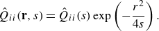 \begin{equation} {\hat {Q}}_{ii}(\mathbf{r},s)={\hat {Q}}_{ii}(s)\exp \left (-\frac {r^2}{4s}\right ) . \end{equation}
By substituting (B11) into (B9), we obtain
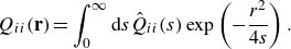 \begin{equation} Q_{ii}(\mathbf{r})=\int _{0}^{\infty }\mathrm{d}s{\hat {Q}}_{ii}(s)\exp \left (-\frac {r^2}{4s}\right ) . \end{equation}
Therefore, the two-point velocity correlation $Q_{ii}(\mathbf{r})$
is expressed in terms of the scale-space energy density
$Q_{ii}(\mathbf{r})$
is expressed in terms of the scale-space energy density ${\hat {Q}}_{ii}(s)$
.
${\hat {Q}}_{ii}(s)$
.
Because the energy density ${\hat {Q}}_{ii}(s)$
is defined analytically as (3.6), we can express the correlation
${\hat {Q}}_{ii}(s)$
is defined analytically as (3.6), we can express the correlation $Q_{ii}(\mathbf{r})$
analytically using know functions as follows. By substituting (3.6) into (B12) and integrating over
$Q_{ii}(\mathbf{r})$
analytically using know functions as follows. By substituting (3.6) into (B12) and integrating over $s$
, we obtain
$s$
, we obtain
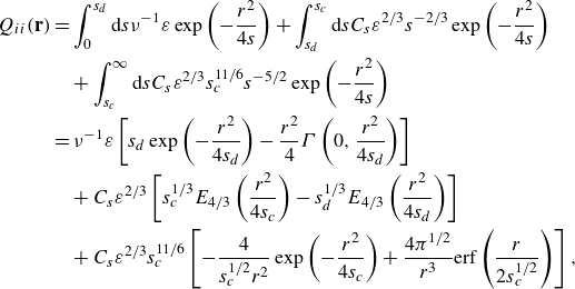 \begin{align} Q_{ii}(\mathbf{r}) &=\int _{0}^{s_d}\mathrm{d}s\nu ^{-1}\varepsilon \exp \left (-\frac {r^2}{4s}\right ) +\int _{s_d}^{s_c}\mathrm{d}sC_s\varepsilon ^{2/3}s^{-2/3}\exp \left (-\frac {r^2}{4s}\right )\nonumber \\ &\quad +\int _{s_c}^{\infty }\mathrm{d}sC_s\varepsilon ^{2/3}s_c^{11/6}s^{-5/2}\exp \left (-\frac {r^2}{4s}\right ) \nonumber \\ &=\nu ^{-1}\varepsilon \left [s_d\exp \left (-\frac {r^2}{4s_d}\right )-\frac {r^2}{4}\Gamma \left (0,\frac {r^2}{4s_d}\right )\right ]\nonumber \\ &\quad +C_s\varepsilon ^{2/3}\left [s_c^{1/3}E_{4/3}\left (\frac {r^2}{4s_c}\right )-s_d^{1/3}E_{4/3}\left (\frac {r^2}{4s_d}\right )\right ] \nonumber \\ &\quad +C_s\varepsilon ^{2/3}s_c^{11/6}\left [-\frac {4}{s_c^{1/2}r^2}\exp \left (-\frac {r^2}{4s_c}\right )+\frac {4\pi ^{1/2}}{r^3}\mathrm{erf}\left (\frac {r}{{2s}_c^{1/2}}\right )\right ] , \end{align}
where $\Gamma (a,x)=\int _{x}^{\infty }\mathrm{d}t\,t^{a-1}\exp (-t)$
is the incomplete gamma function,
$\Gamma (a,x)=\int _{x}^{\infty }\mathrm{d}t\,t^{a-1}\exp (-t)$
is the incomplete gamma function, $E_n(x)=\int _{1}^{\infty }\mathrm{d}t\,t^{-n}\exp (-xt)$
is the exponential integral and
$E_n(x)=\int _{1}^{\infty }\mathrm{d}t\,t^{-n}\exp (-xt)$
is the exponential integral and $\mathrm{erf}(x)=({2}/{\pi ^{1/2}})\int _{0}^{x}\mathrm{d}t\exp (-t^2)$
is the error function.
$\mathrm{erf}(x)=({2}/{\pi ^{1/2}})\int _{0}^{x}\mathrm{d}t\exp (-t^2)$
is the error function.
Appendix C. Effect of molecular diffusivity on Green’s function
For homogeneous isotropic turbulence, the time-dependent part $G(r_x,r_y,r_z,\tau ,y^\prime )$
given by (3.16) can be rewritten as
$G(r_x,r_y,r_z,\tau ,y^\prime )$
given by (3.16) can be rewritten as
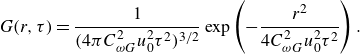 \begin{equation} G(r,\tau )=\frac {1}{(4\pi C_{\omega G}^2u_0^2\tau ^2)^{3/2}}\exp \left (-\frac {r^2}{4C_{\omega G}^2u_0^2\tau ^2}\right ) . \end{equation}
This function represents the solution to the diffusion equation with effective diffusivity $C_{\omega G}^2u_0^2\tau$
. This turbulent diffusion process originates from the transport equation for the Green’s function
$C_{\omega G}^2u_0^2\tau$
. This turbulent diffusion process originates from the transport equation for the Green’s function $g_i(\mathbf{x},t;\mathbf{x}^\prime ,t^\prime )$
given by (A2). The second term on the left-hand side of (A2) involving the velocity fluctuation
$g_i(\mathbf{x},t;\mathbf{x}^\prime ,t^\prime )$
given by (A2). The second term on the left-hand side of (A2) involving the velocity fluctuation $u_{j}$
causes turbulent diffusion with
$u_{j}$
causes turbulent diffusion with $C_{\omega G}^2u_0^2\tau$
. However, for a very small value of
$C_{\omega G}^2u_0^2\tau$
. However, for a very small value of $\tau$
,
$\tau$
, $C_{\omega G}^2u_0^2\tau$
is smaller than the molecular diffusivity
$C_{\omega G}^2u_0^2\tau$
is smaller than the molecular diffusivity $\kappa$
. In this case, the molecular diffusion term in (A2) dominantly contributes to the time evolution of
$\kappa$
. In this case, the molecular diffusion term in (A2) dominantly contributes to the time evolution of $g_i(\mathbf{x},t;\mathbf{x}^\prime ,t^\prime )$
. Rather than the effective diffusivity
$g_i(\mathbf{x},t;\mathbf{x}^\prime ,t^\prime )$
. Rather than the effective diffusivity $C_{\omega G}^2u_0^2\tau$
, the molecular diffusivity
$C_{\omega G}^2u_0^2\tau$
, the molecular diffusivity $\kappa$
is adequate for the diffusion coefficient. To consider the molecular diffusion effect, we can rewrite (C1) as
$\kappa$
is adequate for the diffusion coefficient. To consider the molecular diffusion effect, we can rewrite (C1) as
 \begin{equation} G(r,\tau )=\frac {1}{(4\pi C_{\omega G}^2u_0^2\tau ^2+4\pi \kappa \tau )^{3/2}}\exp \left (-\frac {r^2}{4C_{\omega G}^2u_0^2\tau ^2+4\kappa \tau }\right ) , \end{equation}
by replacing $C_{\omega G}^2u_0^2\tau$
with
$C_{\omega G}^2u_0^2\tau$
with $C_{\omega G}^2u_0^2\tau +\kappa$
. Similarly, for inhomogeneous turbulence, the time-dependent part
$C_{\omega G}^2u_0^2\tau +\kappa$
. Similarly, for inhomogeneous turbulence, the time-dependent part $G(r_x,r_y,r_z,\tau ,y^\prime )$
given by (3.16) is modified by replacing
$G(r_x,r_y,r_z,\tau ,y^\prime )$
given by (3.16) is modified by replacing $R_{ij}$
with
$R_{ij}$
with $R_{ij}+\kappa /(3C_{\omega G}^2\tau )\delta _{ij}$
. Consequently, molecular diffusion with
$R_{ij}+\kappa /(3C_{\omega G}^2\tau )\delta _{ij}$
. Consequently, molecular diffusion with $\kappa$
is dominant in
$\kappa$
is dominant in $G(r_x,r_y,r_z,\tau ,y^\prime )$
for an extremely small value of
$G(r_x,r_y,r_z,\tau ,y^\prime )$
for an extremely small value of $\tau$
. The expression given by (C2) has not yet been verified because only a single Reynolds number with a single value of molecular diffusivity was tested. In future studies, the model will be verified using DNS data of channel flows at different Reynolds and Prandtl numbers.
$\tau$
. The expression given by (C2) has not yet been verified because only a single Reynolds number with a single value of molecular diffusivity was tested. In future studies, the model will be verified using DNS data of channel flows at different Reynolds and Prandtl numbers.


 Open access