


1. Introduction
Compressible turbulent boundary layers (TBLs) over concave surfaces are crucial in configurations such as aerofoils and scramjet engines. The combined effects of concave streamline curvature, adverse pressure gradients and bulk compression in flows over concave surfaces destabilise TBLs to promote turbulent mixing, as highlighted by Bradshaw & Young (Reference Bradshaw and Young1973) and Bradshaw (Reference Bradshaw1974). According to Floryan (Reference Floryan1991), the excited centrifugal effects affect TBLs from three aspects: (i) directly influencing turbulent structures by the wall curvature effect, (ii) generating secondary flows known as Görtler vortices, and (iii) impacting turbulent structures via Görtler vortices. The second effect is also referred to as Görtler instability. However, the behaviours and characteristics of the induced Görtler vortices in turbulent flows remain inadequately understood compared to those in laminar flows.
Early studies focused on experiments to explore the impact of concave curvature $ K=\delta /r$
on turbulence, where
$ K=\delta /r$
on turbulence, where $ \delta$
is the boundary-layer thickness, and
$ \delta$
is the boundary-layer thickness, and $ r$
is the curvature radius. Hoffmann, Muck & Bradshaw (Reference Hoffmann, Muck and Bradshaw1985) experimentally investigated the impact of curvature on incompressible TBLs. They concluded that the wall curvature directly dominates turbulent structures when the curvature is not strong enough, while the Görtler vortices are more influential at a moderate curvature
$ r$
is the curvature radius. Hoffmann, Muck & Bradshaw (Reference Hoffmann, Muck and Bradshaw1985) experimentally investigated the impact of curvature on incompressible TBLs. They concluded that the wall curvature directly dominates turbulent structures when the curvature is not strong enough, while the Görtler vortices are more influential at a moderate curvature $ K=\delta /r\geqslant 0.01$
. The critical value suggests that strong curvature is necessary to form Görtler vortices due to fuller TBLs (Floryan Reference Floryan1991). In supersonic flows, Jayaram, Taylor & Smits (Reference Jayaram, Taylor and Smits1987) compared TBLs over concave surfaces with curvatures 0.02 and 0.1 to those over a compression ramp (
$ K=\delta /r\geqslant 0.01$
. The critical value suggests that strong curvature is necessary to form Görtler vortices due to fuller TBLs (Floryan Reference Floryan1991). In supersonic flows, Jayaram, Taylor & Smits (Reference Jayaram, Taylor and Smits1987) compared TBLs over concave surfaces with curvatures 0.02 and 0.1 to those over a compression ramp ( $ K\rightarrow \infty$
) with the same turning angle
$ K\rightarrow \infty$
) with the same turning angle $ 8^\circ$
. The study revealed that turbulent fluctuations respond rapidly in regions with large curvature to alter turbulent structures. The authors also reported a dip below the logarithmic law, but did not detect longitudinal roll cells in their experiments. Later, Barlow & Johnston (Reference Barlow and Johnston1988a
,Reference Barlow and Johnston
b
) observed that longitudinal roll cells wander side to side without preferred spanwise locations when the freestream is relatively free of spanwise non-uniformities, indicating that these roll cells are unsteady. However, a stationary pattern of large-scale roll cells was found when introducing steady weak disturbances using small vortex generators. These stable structures were observed in time-averaged visualisations with the spanwise wavelength approximately 1–2 times the boundary-layer thickness. A similar steady pattern with the help of upstream vortex generators was also discussed by Schuelein & Trofimov (Reference Schuelein and Trofimov2011) in supersonic compression ramp cases. Different patterns of the large-scale motions highlight the influence of upstream disturbances, as summarised by Floryan (Reference Floryan1991) and Priebe et al. (Reference Priebe, Tu, Rowley and Martín2016). Donovan, Spina & Smits (Reference Donovan, Spina and Smits1994) investigated the response of the large-scale motions to a short concave region but with a strong concave curvature
$ 8^\circ$
. The study revealed that turbulent fluctuations respond rapidly in regions with large curvature to alter turbulent structures. The authors also reported a dip below the logarithmic law, but did not detect longitudinal roll cells in their experiments. Later, Barlow & Johnston (Reference Barlow and Johnston1988a
,Reference Barlow and Johnston
b
) observed that longitudinal roll cells wander side to side without preferred spanwise locations when the freestream is relatively free of spanwise non-uniformities, indicating that these roll cells are unsteady. However, a stationary pattern of large-scale roll cells was found when introducing steady weak disturbances using small vortex generators. These stable structures were observed in time-averaged visualisations with the spanwise wavelength approximately 1–2 times the boundary-layer thickness. A similar steady pattern with the help of upstream vortex generators was also discussed by Schuelein & Trofimov (Reference Schuelein and Trofimov2011) in supersonic compression ramp cases. Different patterns of the large-scale motions highlight the influence of upstream disturbances, as summarised by Floryan (Reference Floryan1991) and Priebe et al. (Reference Priebe, Tu, Rowley and Martín2016). Donovan, Spina & Smits (Reference Donovan, Spina and Smits1994) investigated the response of the large-scale motions to a short concave region but with a strong concave curvature $ K = 0.08$
. They reported that the centrifugal effects amplify turbulence levels and skin friction compared to flat plates with similar pressure distributions. Later, Wang & Wang (Reference Wang and Wang2016) analysed the break-up process in the concave region from large-scale structures to smaller ones with high-resolution flow visualisation, finding that the vortices tend to break up faster under more significant concave curvature.
$ K = 0.08$
. They reported that the centrifugal effects amplify turbulence levels and skin friction compared to flat plates with similar pressure distributions. Later, Wang & Wang (Reference Wang and Wang2016) analysed the break-up process in the concave region from large-scale structures to smaller ones with high-resolution flow visualisation, finding that the vortices tend to break up faster under more significant concave curvature.
In recent years, high-fidelity numerical simulations have been employed to investigate turbulent structures over concave surfaces. Tong et al. (Reference Tong, Li, Duan and Yu2017) performed direct numerical simulations (DNS) to study supersonic TBLs over a curved ramp with $ K=0.02$
and turning angle
$ K=0.02$
and turning angle $ \varphi =24^{\circ }$
at Mach 2.95. They discovered a mode at
$ \varphi =24^{\circ }$
at Mach 2.95. They discovered a mode at $ f\delta /{u}_{\infty } =0.017$
with regular spatial structures distributed in the spanwise direction using dynamic mode decomposition, where
$ f\delta /{u}_{\infty } =0.017$
with regular spatial structures distributed in the spanwise direction using dynamic mode decomposition, where $ {u}_{\infty }$
is the freestream velocity. These structures resemble the spanwise structures of Görtler vortices in laminar flows. Sun, Sandham & Hu (Reference Sun, Sandham and Hu2019) compared TBLs over concave surfaces with two different radii to those over a flat plate, and reported prominent low-frequency fluctuations (within the range
$ {u}_{\infty }$
is the freestream velocity. These structures resemble the spanwise structures of Görtler vortices in laminar flows. Sun, Sandham & Hu (Reference Sun, Sandham and Hu2019) compared TBLs over concave surfaces with two different radii to those over a flat plate, and reported prominent low-frequency fluctuations (within the range $ f\delta /{u}_{\infty } =0.2{-}0.4$
) on concave surfaces due to large-scale structures. They noted that Görtler instability primarily affects the outer layer, forming Görtler-like vortices, while the inner layer remains largely unaffected. These vortices facilitate rapid momentum exchange between the inner and outer parts of TBLs, enhancing turbulence intensity and Reynolds stresses. Wang et al. (Reference Wang, Wang, Sun, Yang, Zhao and Hu2019) also observed similar momentum exchange processes driven by large-scale roll cells, achieved through ejection and sweep events that transport high-momentum flow towards the wall, and low-momentum flow towards the outer edge. They suggested that these large-scale roll cells originate from very-large-scale motions in the absence of upstream artificial disturbances. Wu, Liang & Zhao (Reference Wu, Liang and Zhao2019) numerically investigated the small curvature case studied by Jayaram et al. (Reference Jayaram, Taylor and Smits1987) at
$ f\delta /{u}_{\infty } =0.2{-}0.4$
) on concave surfaces due to large-scale structures. They noted that Görtler instability primarily affects the outer layer, forming Görtler-like vortices, while the inner layer remains largely unaffected. These vortices facilitate rapid momentum exchange between the inner and outer parts of TBLs, enhancing turbulence intensity and Reynolds stresses. Wang et al. (Reference Wang, Wang, Sun, Yang, Zhao and Hu2019) also observed similar momentum exchange processes driven by large-scale roll cells, achieved through ejection and sweep events that transport high-momentum flow towards the wall, and low-momentum flow towards the outer edge. They suggested that these large-scale roll cells originate from very-large-scale motions in the absence of upstream artificial disturbances. Wu, Liang & Zhao (Reference Wu, Liang and Zhao2019) numerically investigated the small curvature case studied by Jayaram et al. (Reference Jayaram, Taylor and Smits1987) at $ K=0.02$
and
$ K=0.02$
and $ \varphi =8^{\circ }$
, but with a lower reference Reynolds number. They found that the outer peak of the energy spectra falls in the lower-wake region due to the turbulence amplification effect. However, they demonstrated that log-region superstructures primarily contribute to outer–inner interactions in the concave region, i.e. large/small-scale interactions, enhancing turbulence modulation strength significantly. In a recent study, Tong et al. (Reference Tong, Duan, Ji, Dong, Yuan and Li2023) carried out DNS to characterise the effect of concave curvature on the wall shear stress and heat flux. They emphasised the leading role of the outer large-scale structures in contributing to the mean wall shear stress and wall heat flux.
$ \varphi =8^{\circ }$
, but with a lower reference Reynolds number. They found that the outer peak of the energy spectra falls in the lower-wake region due to the turbulence amplification effect. However, they demonstrated that log-region superstructures primarily contribute to outer–inner interactions in the concave region, i.e. large/small-scale interactions, enhancing turbulence modulation strength significantly. In a recent study, Tong et al. (Reference Tong, Duan, Ji, Dong, Yuan and Li2023) carried out DNS to characterise the effect of concave curvature on the wall shear stress and heat flux. They emphasised the leading role of the outer large-scale structures in contributing to the mean wall shear stress and wall heat flux.
Previous studies have primarily examined the effects of concave curvature on turbulent statistical properties, emphasising how wall curvature and Görtler vortices significantly alter turbulent structures. However, the Görtler vortices themselves in turbulent flows, particularly their spatial–temporal structures and scales, remain poorly understood. These vortices, characterised by counter-rotating roll cells in laminar flows, are challenging to visualise in turbulent flows due to the presence of complex small-scale structures (Wang et al. Reference Wang, Wang, Sun, Yang, Zhao and Hu2019). Additionally, while many studies have shown that the spanwise wavelength of Görtler vortices is typically approximately $ 2\delta$
, Guo et al. (Reference Guo, Zhang, Zhu and Li2024) also reported structures with spanwise wavelength approximately
$ 2\delta$
, Guo et al. (Reference Guo, Zhang, Zhu and Li2024) also reported structures with spanwise wavelength approximately $ 1.2\delta$
. Therefore, the spanwise scales of Görtler vortices also need to be thoroughly examined.
$ 1.2\delta$
. Therefore, the spanwise scales of Görtler vortices also need to be thoroughly examined.
In recent years, resolvent analysis (McKeon & Sharma Reference McKeon and Sharma2010) has become an attractive tool for studying coherent structures in turbulent flows. This method identifies the most amplified response for a given input forcing, and has been successfully applied to predict coherent structures in turbulent jets (Schmidt et al. Reference Schmidt, Towne, Rigas, Colonius and Brès2018; Lesshafft et al. Reference Lesshafft, Semeraro, Jaunet, Cavalieri and Jordan2019; Maia et al. Reference Maia, Heidt, Pickering, Colonius, Jordan and Brès2024) and channel flows (McKeon Reference McKeon2017; Bae, Dawson & McKeon Reference Bae, Dawson and McKeon2020; Fan et al. Reference Fan, Kozul, Li and Sandberg2024), as well as to investigate the low-frequency dynamics of turbulent separation bubbles (Hao Reference Hao2023; Cura et al. Reference Cura, Hanifi, Cavalieri and Weiss2024).
The present study aims to investigate the features of Görtler vortices in supersonic turbulent flows using resolvent analysis and large-eddy simulations (LES). We will focus on the spatial–temporal structures and spanwise scales of these vortices. Resolvent analysis will be used to predict the most amplified coherent structures on concave surfaces. These predictions will be compared with structures extracted by proper orthogonal decomposition (POD) and spectral proper orthogonal decomposition (SPOD) based on the LES dataset. We expect the predicted structures to be Görtler vortices, with Görtler instability as the dominant amplification mechanism. Finally, we will explore how geometric and freestream parameters influence the preferential spanwise scale of Görtler vortices and predict their occurrence.
2. Geometry and freestream conditions
As sketched in figure 1, the flow configuration in this study involves a concave surface with total turning angle $ \varphi =20^{\circ }$
and curvature radius
$ \varphi =20^{\circ }$
and curvature radius $ r=50 \delta$
(
$ r=50 \delta$
( $ K=0.02$
). A Cartesian coordinate system is established with the origin at the beginning of the concave surface. The computational domains for the Reynolds-averaged Navier–Stokes (RANS) simulations and LES are also marked in the figure. The freestream parameters are taken from Zheltovodov et al. (Reference Zheltovodov, Trofimov, Schülein and Yakovlev1990), with Mach number
$ K=0.02$
). A Cartesian coordinate system is established with the origin at the beginning of the concave surface. The computational domains for the Reynolds-averaged Navier–Stokes (RANS) simulations and LES are also marked in the figure. The freestream parameters are taken from Zheltovodov et al. (Reference Zheltovodov, Trofimov, Schülein and Yakovlev1990), with Mach number $ {M}_{\infty }=2.95$
, density
$ {M}_{\infty }=2.95$
, density $ {\rho }_{\infty }=0.314$
kg m
$ {\rho }_{\infty }=0.314$
kg m $^{-3}$
, statistic temperature
$^{-3}$
, statistic temperature $ {T}_{\infty }=108$
K, and Reynolds number
$ {T}_{\infty }=108$
K, and Reynolds number $ {Re}_{\delta }=63\,500$
with
$ {Re}_{\delta }=63\,500$
with $ \delta = 2.27$
mm. The boundary-layer thickness
$ \delta = 2.27$
mm. The boundary-layer thickness $ \delta$
is defined as
$ \delta$
is defined as $ 99\, \%$
of the freestream velocity at the reference station
$ 99\, \%$
of the freestream velocity at the reference station $ x_{0}$
(see figure 1).
$ x_{0}$
(see figure 1).
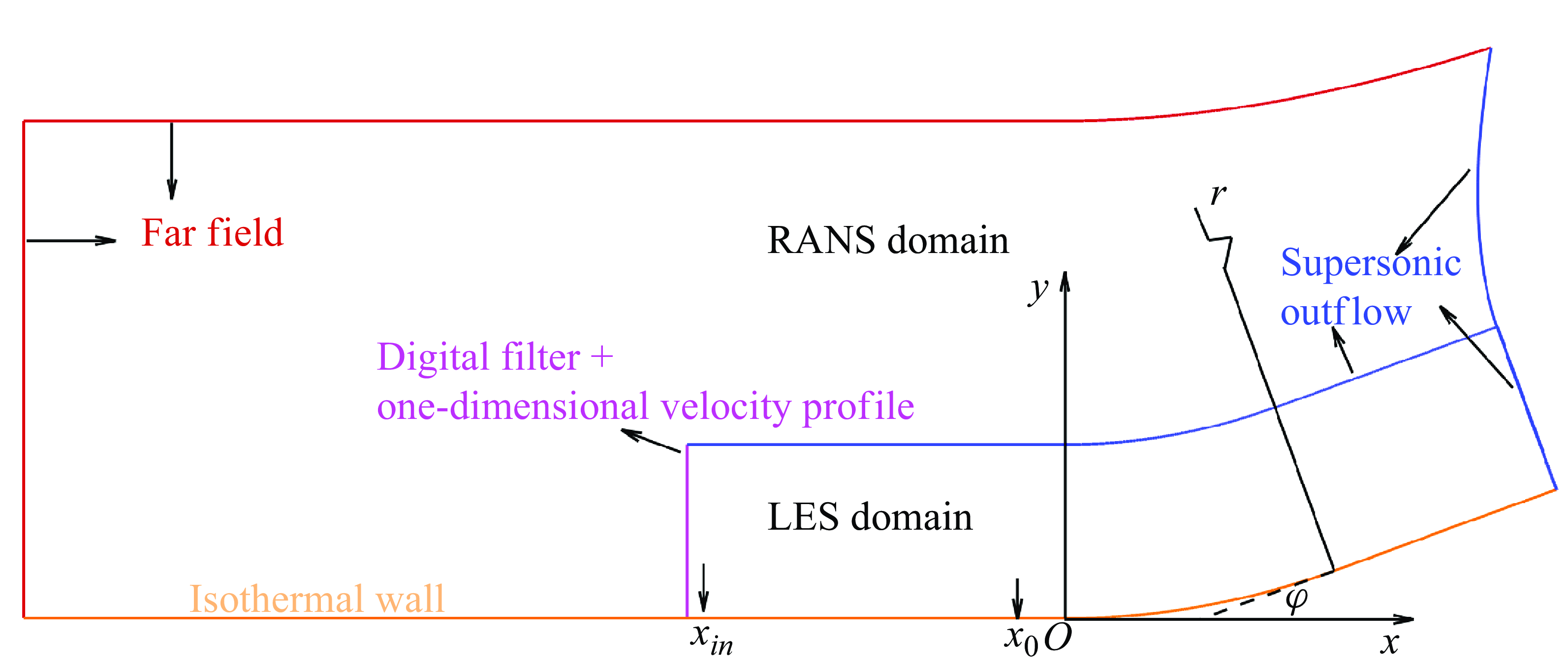
Figure 1. Computational domains and boundary conditions: $ r$
is the curvature radius,
$ r$
is the curvature radius, $ \varphi$
is the turning angle,
$ \varphi$
is the turning angle, $ x_{0}$
is at
$ x_{0}$
is at $ (-1.76\delta ,0)$
, the reference station, and
$ (-1.76\delta ,0)$
, the reference station, and $ x_{in}$
is at
$ x_{in}$
is at $(-22.5\delta ,0)$
, the station of the chosen one-dimensional velocity profile from the RANS base flow. The RANS domain and LES domain refer to the computation domains for RANS simulations and LES, respectively. Boundary conditions for RANS and LES are also marked.
$(-22.5\delta ,0)$
, the station of the chosen one-dimensional velocity profile from the RANS base flow. The RANS domain and LES domain refer to the computation domains for RANS simulations and LES, respectively. Boundary conditions for RANS and LES are also marked.
3. Theoretical and numerical approach
3.1. Governing equations
The compressible Navier–Stokes equations in operator form are given as
 \begin{equation} \frac {\partial \boldsymbol{U}}{\partial t}=\boldsymbol{\mathcal{N}}(\boldsymbol{U}), \end{equation}
where $ \boldsymbol{U}$
is the vector of conservative variables, and
$ \boldsymbol{U}$
is the vector of conservative variables, and $ \boldsymbol{\mathcal{N}}$
denotes the nonlinear Navier–Stokes operator. For the RANS equations,
$ \boldsymbol{\mathcal{N}}$
denotes the nonlinear Navier–Stokes operator. For the RANS equations, $ \boldsymbol{U}$
is the vector of Favre-averaged variables, and
$ \boldsymbol{U}$
is the vector of Favre-averaged variables, and $ \boldsymbol{\mathcal{N}}$
is the nonlinear RANS operator. In the case of LES, the governing equations are the Favre-filtered Navier–Stokes equations, with
$ \boldsymbol{\mathcal{N}}$
is the nonlinear RANS operator. In the case of LES, the governing equations are the Favre-filtered Navier–Stokes equations, with $ \boldsymbol{U}$
representing the vector of Favre-filtered variables, and
$ \boldsymbol{U}$
representing the vector of Favre-filtered variables, and $ \boldsymbol{\mathcal{N}}$
representing the nonlinear LES operator. The Favre filter is defined as
$ \boldsymbol{\mathcal{N}}$
representing the nonlinear LES operator. The Favre filter is defined as $ \langle f \rangle =\overline {\rho f} /\bar {\rho }$
, where an overline denotes the spatial filter (Garnier, Adams & Sagaut Reference Garnier, Adams and Sagaut2009).
$ \langle f \rangle =\overline {\rho f} /\bar {\rho }$
, where an overline denotes the spatial filter (Garnier, Adams & Sagaut Reference Garnier, Adams and Sagaut2009).
The working fluid is assumed to be a perfect gas with Prandtl number $ Pr=0.72$
and specific heat ratio 1.4. The molecular viscosity
$ Pr=0.72$
and specific heat ratio 1.4. The molecular viscosity $ \mu$
is calculated from Sutherland’s law, and the turbulent Prandtl number
$ \mu$
is calculated from Sutherland’s law, and the turbulent Prandtl number $ Pr_{t}$
is chosen to be 0.9.
$ Pr_{t}$
is chosen to be 0.9.
3.2. The RANS solver
The Boussinesq assumption is employed in the RANS equations to model the Reynolds stresses, with the eddy viscosity $ \mu _{t}$
obtained from the Spalart–Allmaras turbulence model (Spalart & Allmaras Reference Spalart and Allmaras1992). An in-house finite-volume solver called PHAROS (Hao, Wang & Lee Reference Hao, Wang and Lee2016; Hao & Wen Reference Hao and Wen2020) is used to obtain RANS base flows. The modified Steger–Warming scheme (MacCormack Reference MacCormack2014) is applied in computing the inviscid fluxes, and the viscous fluxes are solved using a second-order central difference scheme. The implicit line relaxation method proposed by Wright, Candler & Bose (Reference Wright, Candler and Bose1998) is employed for pseudo-time marching. The computation domain and boundary conditions are also marked in figure 1. The far-field boundaries follow the freestream conditions. The supersonic outflow boundary uses a simple extrapolation, and an isothermal no-slip condition with fixed temperature
$ \mu _{t}$
obtained from the Spalart–Allmaras turbulence model (Spalart & Allmaras Reference Spalart and Allmaras1992). An in-house finite-volume solver called PHAROS (Hao, Wang & Lee Reference Hao, Wang and Lee2016; Hao & Wen Reference Hao and Wen2020) is used to obtain RANS base flows. The modified Steger–Warming scheme (MacCormack Reference MacCormack2014) is applied in computing the inviscid fluxes, and the viscous fluxes are solved using a second-order central difference scheme. The implicit line relaxation method proposed by Wright, Candler & Bose (Reference Wright, Candler and Bose1998) is employed for pseudo-time marching. The computation domain and boundary conditions are also marked in figure 1. The far-field boundaries follow the freestream conditions. The supersonic outflow boundary uses a simple extrapolation, and an isothermal no-slip condition with fixed temperature $ 275.4$
K is applied to the wall.
$ 275.4$
K is applied to the wall.
3.3. The LES solver
Implicit LES are also conducted using PHAROS. The low-dissipative sixth-order kinetic preserving scheme (Pirozzoli Reference Pirozzoli2010) combining the AUSM $ ^{+}$
-up scheme (Liou Reference Liou2006) with the fifth-order weighted essentially non-oscillatory reconstruction (Jiang & Shu Reference Jiang and Shu1996) is used to solve the inviscid fluxes, switched by the Jameson sensor (Jameson, Schmidt & Turkel Reference Jameson, Schmidt and Turkel1981). Time integration is performed using a third-order low-storage Runge–Kutta scheme, with time step
$ ^{+}$
-up scheme (Liou Reference Liou2006) with the fifth-order weighted essentially non-oscillatory reconstruction (Jiang & Shu Reference Jiang and Shu1996) is used to solve the inviscid fluxes, switched by the Jameson sensor (Jameson, Schmidt & Turkel Reference Jameson, Schmidt and Turkel1981). Time integration is performed using a third-order low-storage Runge–Kutta scheme, with time step $ 9$
ns. The total simulation time is approximately 10 ms. Flow samples are collected for duration 8.1 ms (
$ 9$
ns. The total simulation time is approximately 10 ms. Flow samples are collected for duration 8.1 ms ( $ 2200 \delta /u_{\infty }$
).
$ 2200 \delta /u_{\infty }$
).
The computational domain for LES is reduced appropriately, as depicted in figure 1. The spanwise width of the domain is set as $ 6\delta$
. The inflow boundary employs the extended digital filter technology (Touber & Sandham Reference Touber and Sandham2009; Ceci et al. Reference Ceci, Palumbo, Larsson and Pirozzoli2022) and a one-dimensional profile extracted from the RANS base flow, as marked at station
$ 6\delta$
. The inflow boundary employs the extended digital filter technology (Touber & Sandham Reference Touber and Sandham2009; Ceci et al. Reference Ceci, Palumbo, Larsson and Pirozzoli2022) and a one-dimensional profile extracted from the RANS base flow, as marked at station $ x_{in}$
at
$ x_{in}$
at $ (-22.5\delta ,0)$
in figure 1. The profile is chosen to ensure that the boundary-layer thickness
$ (-22.5\delta ,0)$
in figure 1. The profile is chosen to ensure that the boundary-layer thickness $ \delta$
at station
$ \delta$
at station $ x_{0}$
is 2.27 mm after a turbulence recovery process. Supersonic outflow boundary conditions are specified at the upper and right boundaries. The grid is progressively coarsened at these boundaries, combined with a sponge zone of thickness approximately
$ x_{0}$
is 2.27 mm after a turbulence recovery process. Supersonic outflow boundary conditions are specified at the upper and right boundaries. The grid is progressively coarsened at these boundaries, combined with a sponge zone of thickness approximately $ 3\delta$
near the upper boundary to damp the flow variables to the freestream values to avoid any reflections (Mani Reference Mani2012). Periodic boundary conditions are used in the spanwise direction. The wall is assumed to be no-slip and isothermal with
$ 3\delta$
near the upper boundary to damp the flow variables to the freestream values to avoid any reflections (Mani Reference Mani2012). Periodic boundary conditions are used in the spanwise direction. The wall is assumed to be no-slip and isothermal with $ T_{w}=275.4$
K. The grid measures
$ T_{w}=275.4$
K. The grid measures $1423 \times181\times301$
in the streamwise, wall-normal and spanwise directions, respectively. The mesh is uniform in the streamwise and spanwise directions, with grid resolutions
$1423 \times181\times301$
in the streamwise, wall-normal and spanwise directions, respectively. The mesh is uniform in the streamwise and spanwise directions, with grid resolutions $ \Delta x^{+}\approx 19$
,
$ \Delta x^{+}\approx 19$
, $\Delta {y}_{w}^{+}\approx 1.0$
and
$\Delta {y}_{w}^{+}\approx 1.0$
and $ \Delta z^{+}\approx 9$
at the reference station
$ \Delta z^{+}\approx 9$
at the reference station $ x_{0}$
.
$ x_{0}$
.
3.4. Resolvent analysis
Resolvent analysis is based on the scale separation assumption, which posits a sufficient scale gap between large-scale coherent structures and turbulent fluctuations. Globally stable flows can be modelled as a noise amplifier (Huerre & Monkewitz Reference Huerre and Monkewitz1990) and investigated using resolvent analysis (Sipp & Marquet Reference Sipp and Marquet2013). To study the linear forced dynamics of a noise amplifier flow, a small-amplitude forcing $ \boldsymbol{f}^{\prime}$
is introduced into the linearised Navier–Stokes equations, given as
$ \boldsymbol{f}^{\prime}$
is introduced into the linearised Navier–Stokes equations, given as
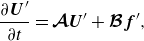 \begin{equation} \frac {\partial \boldsymbol{U}^{\prime}}{\partial t}=\boldsymbol{\mathcal{A}U}^{\prime}+\boldsymbol{\mathcal{B}f}^{\prime}, \end{equation}
where $ \boldsymbol{\mathcal{A}}$
is the linearised operator evaluated using a base flow from RANS results or LES Favre-averaged results, and
$ \boldsymbol{\mathcal{A}}$
is the linearised operator evaluated using a base flow from RANS results or LES Favre-averaged results, and $ \boldsymbol{U}^{\prime}$
is the perturbation term around the base flow. The operator
$ \boldsymbol{U}^{\prime}$
is the perturbation term around the base flow. The operator $ \boldsymbol{\mathcal{B}}$
is to constrain the forcing field to a localised region (Bugeat et al. Reference Bugeat, Chassaing, Robinet and Sagaut2019). Both
$ \boldsymbol{\mathcal{B}}$
is to constrain the forcing field to a localised region (Bugeat et al. Reference Bugeat, Chassaing, Robinet and Sagaut2019). Both $ \boldsymbol{U}^{\prime}$
and
$ \boldsymbol{U}^{\prime}$
and $ \boldsymbol{f}^{\prime}$
are assumed to be harmonic in time and the spanwise direction, given as
$ \boldsymbol{f}^{\prime}$
are assumed to be harmonic in time and the spanwise direction, given as
 \begin{align} \boldsymbol{U}^{\prime}(x,y,z,t) & =\hat {\boldsymbol{U}}(x,y)\exp(i\beta z-i{\omega }_{r}t), \nonumber\\ \boldsymbol{f}^{\prime}(x,y,z,t) & =\,\hat {\boldsymbol{\!\!f}}(x,y)\exp(i\beta z-i{\omega }_{r}t), \end{align}
where $ \beta$
is the spanwise wavenumber, and
$ \beta$
is the spanwise wavenumber, and $ \omega _{r}$
is the angular frequency. Substituting (3.3) into (3.2) gives
$ \omega _{r}$
is the angular frequency. Substituting (3.3) into (3.2) gives
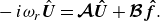 \begin{equation} -i{\omega }_{r}\hat {\boldsymbol{U}}=\boldsymbol{\mathcal{A}\hat {U}}+\boldsymbol{\mathcal{B}\hat {f}}. \end{equation}
Introducing the resolvent operator $ \boldsymbol{\mathcal{R}}={(-{i\omega }_{r}\boldsymbol{\mathcal{I}}-\boldsymbol{\mathcal{A}})}^{-1}$
and the identity operator
$ \boldsymbol{\mathcal{R}}={(-{i\omega }_{r}\boldsymbol{\mathcal{I}}-\boldsymbol{\mathcal{A}})}^{-1}$
and the identity operator $ \boldsymbol{\mathcal{I}}$
, (3.4) can be written as a relationship between the constrained forcing and its linear response, given by
$ \boldsymbol{\mathcal{I}}$
, (3.4) can be written as a relationship between the constrained forcing and its linear response, given by
 \begin{equation} \hat{\boldsymbol{U}}=\boldsymbol{\mathcal{R}}\boldsymbol{\mathcal{B}}\,\,\hat {\boldsymbol{\!\!f}}. \end{equation}
To seek the most energetic amplification between the forcing and the response, the optimal gain $ \sigma$
is defined as
$ \sigma$
is defined as
 \begin{equation} {\sigma }^{2}({\omega }_{r},\beta )=\max _{\hat {f}}{\frac {{\| \boldsymbol{\hat {U}}\| }_{E}^{2} }{{\| \boldsymbol{{\hat {f}}}\| }_{E}^{2}}}. \end{equation}
The Chu energy norm (Chu Reference Chu1965) is applied to the response and the forcing to evaluate their respective energies. As discussed by Bugeat et al. (Reference Bugeat, Chassaing, Robinet and Sagaut2019), (3.6) can be converted to an eigenvalue problem. The problem is discretised similarly to the flow solver, except that a central scheme is used to solve the inviscid fluxes in smooth regions detected by a shock sensor (Hendrickson, Kartha & Candler Reference Hendrickson, Kartha and Candler2018). At the left-hand and upper boundaries, all perturbations are set to zero. At the right-hand boundary, a simple extrapolation is used. The wall conditions are $ u^{\prime}=v^{\prime}=w^{\prime}=0$
,
$ u^{\prime}=v^{\prime}=w^{\prime}=0$
, $ T^{\prime}=0$
and
$ T^{\prime}=0$
and $ \partial p^{\prime}/\partial n =0$
. Sponge zones with thickness
$ \partial p^{\prime}/\partial n =0$
. Sponge zones with thickness $ 5\delta$
are implemented to the left-hand, right-hand and upper boundaries to gradually damp the perturbations to zero (Mani Reference Mani2012). Finally, the implicitly restarted Arnoldi method implemented in ARPACK (Lehoucq, Sorensen & Yang 1996), interfaced with the MUMPS (Amestoy et al. Reference Amestoy, Duff, L’Excellent and Koster2001) open library, is used to solve the eigenvalue problems.
$ 5\delta$
are implemented to the left-hand, right-hand and upper boundaries to gradually damp the perturbations to zero (Mani Reference Mani2012). Finally, the implicitly restarted Arnoldi method implemented in ARPACK (Lehoucq, Sorensen & Yang 1996), interfaced with the MUMPS (Amestoy et al. Reference Amestoy, Duff, L’Excellent and Koster2001) open library, is used to solve the eigenvalue problems.
It should be noted that the resolvent analysis solver adapted is for laminar flows (Hao et al. Reference Hao, Cao, Guo and Wen2023), while incorporating the effective viscosity $ \mu _{eff}=\mu +\mu _{t}$
and effective heat conductivity
$ \mu _{eff}=\mu +\mu _{t}$
and effective heat conductivity $ k_{eff}=\mu /Pr+\mu _{t}/Pr_{t}$
to model turbulent fluctuations (Fan et al. Reference Fan, Kozul, Li and Sandberg2024). The explicit expressions of the operators
$ k_{eff}=\mu /Pr+\mu _{t}/Pr_{t}$
to model turbulent fluctuations (Fan et al. Reference Fan, Kozul, Li and Sandberg2024). The explicit expressions of the operators $ \boldsymbol{\mathcal{A}}$
,
$ \boldsymbol{\mathcal{A}}$
, $ \boldsymbol{\mathcal{B}}$
and
$ \boldsymbol{\mathcal{B}}$
and $ \boldsymbol{\mathcal{R}}$
in laminar flows can be found in Bugeat et al. (Reference Bugeat, Chassaing, Robinet and Sagaut2019). In this study, the perturbation of
$ \boldsymbol{\mathcal{R}}$
in laminar flows can be found in Bugeat et al. (Reference Bugeat, Chassaing, Robinet and Sagaut2019). In this study, the perturbation of $ \mu _{t}$
is not considered, meaning that
$ \mu _{t}$
is not considered, meaning that $ \mu _{t}$
is assumed to be frozen everywhere, consistent with Cura et al. (Reference Cura, Hanifi, Cavalieri and Weiss2024).
$ \mu _{t}$
is assumed to be frozen everywhere, consistent with Cura et al. (Reference Cura, Hanifi, Cavalieri and Weiss2024).
3.5. Local stability analysis
In local stability analysis (LSA), the perturbation $ \boldsymbol{U}^{\prime}$
is expressed as
$ \boldsymbol{U}^{\prime}$
is expressed as
 \begin{equation} \boldsymbol{U}^{\prime}(x,y,z,t)=\hat {\boldsymbol{U}}_{1\text{-}D}(y)\exp\left [i(\alpha _{r}+i\alpha _{i})x+i\beta z-i{\omega }_{r}t \right ], \end{equation}
where $ \hat {\boldsymbol{U}}_{1\text{-}D}(y)$
is the one-dimensional eigenfunction,
$ \hat {\boldsymbol{U}}_{1\text{-}D}(y)$
is the one-dimensional eigenfunction, $ \alpha _{r}$
is the real streamwise wavenumber, and
$ \alpha _{r}$
is the real streamwise wavenumber, and $ \alpha _{i}$
is the spatial growth rate. A negative value of
$ \alpha _{i}$
is the spatial growth rate. A negative value of $ \alpha _{i}$
indicates that the corresponding mode is unstable. Notably, the effective viscosity
$ \alpha _{i}$
indicates that the corresponding mode is unstable. Notably, the effective viscosity $ {\mu }_{eff}$
and the concave curvature
$ {\mu }_{eff}$
and the concave curvature $ K$
(Ren & Fu Reference Ren and Fu2014) are adopted to conduct LSA. Substituting (3.7) into the linearised Navier–Stokes equations yields an eigenvalue problem, which is solved using the Eigen (Guennebaud, Jacob & Reference Guennebaud2010) library at given values of
$ K$
(Ren & Fu Reference Ren and Fu2014) are adopted to conduct LSA. Substituting (3.7) into the linearised Navier–Stokes equations yields an eigenvalue problem, which is solved using the Eigen (Guennebaud, Jacob & Reference Guennebaud2010) library at given values of $ \beta$
and
$ \beta$
and $ {\omega }_{r}$
. The boundary conditions are consistent with those in § 3.2.
$ {\omega }_{r}$
. The boundary conditions are consistent with those in § 3.2.
3.6. Spectral proper orthogonal decomposition
Spectral proper orthogonal decomposition (Lumley Reference Lumley1967; Towne, Schmidt & Colonius Reference Towne, Schmidt and Colonius2018; Schmidt et al. Reference Schmidt, Towne, Rigas, Colonius and Brès2018) extracts coherent structures from the perspective of energy from flow data. It seeks a set of orthogonal bases to represent the overall power spectra in time and space optimally. Hence SPOD is ideal for identifying coherent structures in turbulent flows.
The key point in SPOD is to accurately estimate the cross-spectral density (CSD) tensor from a time series (Towne et al. Reference Towne, Schmidt and Colonius2018). The CSD matrix at each frequency is estimated by
 \begin{equation} \boldsymbol{\hat {S}}(\omega _{k})=\boldsymbol{\hat {Q}}(\omega _{k})\boldsymbol{\cdot} {\boldsymbol{\hat {Q}}^{*}}(\omega _{k}), \end{equation}
where $ \boldsymbol{\hat {Q}}(\omega _{k})$
is the data matrix at
$ \boldsymbol{\hat {Q}}(\omega _{k})$
is the data matrix at $ k$
th frequency
$ k$
th frequency $ \omega _{k}$
, and
$ \omega _{k}$
, and $ (\cdot )^{*}$
is the Hermitian transpose. The problem is transformed to a series of eigenvalue problems at frequency
$ (\cdot )^{*}$
is the Hermitian transpose. The problem is transformed to a series of eigenvalue problems at frequency $ \omega _{k}$
, given as
$ \omega _{k}$
, given as
 \begin{equation} \boldsymbol{\hat {S}W\hat {\Psi }}=\boldsymbol{\hat {\Psi }\hat {\Lambda }}, \end{equation}
or via the method of snapshots,
 \begin{equation} \boldsymbol{\hat {Q}}^{*} \boldsymbol{W} \hat{\boldsymbol{\!Q}} \hat {\boldsymbol{\Theta}}=\boldsymbol{\hat {\Theta }} \hat {\boldsymbol{\Lambda} },\quad\boldsymbol{\hat {\Psi }} =\boldsymbol{\hat {Q}}\hat {\boldsymbol{\Theta }}, \end{equation}
where $ \boldsymbol{W}$
is the weight matrix,
$ \boldsymbol{W}$
is the weight matrix, $ \boldsymbol{\hat {\!\Lambda } }$
gives the eigenvalues, and the SPOD modes
$ \boldsymbol{\hat {\!\Lambda } }$
gives the eigenvalues, and the SPOD modes $ \boldsymbol{\hat {\Psi }}$
are recovered using the eigenvectors
$ \boldsymbol{\hat {\Psi }}$
are recovered using the eigenvectors $ \boldsymbol{\hat {\Theta }}$
. The Chu energy norm (Chu Reference Chu1965) is commonly used in the weight matrix
$ \boldsymbol{\hat {\Theta }}$
. The Chu energy norm (Chu Reference Chu1965) is commonly used in the weight matrix $ \boldsymbol{W}$
for compressible flows.
$ \boldsymbol{W}$
for compressible flows.
Of particular interest is the most energetic SPOD mode, which corresponds to the largest eigenvalue, often referred to as the optimal or leading SPOD mode. A low-rank feature is observed when the optimal eigenvalue is significantly larger than the others. In this scenario, the physical mechanism associated with the optimal mode becomes dominant and prevalent (Schmidt et al. Reference Schmidt, Towne, Rigas, Colonius and Brès2018).
4. Spatial–temporal structures
4.1. Response to upstream disturbances
Figure 2 presents the Mach number contour of the time- and spanwise-averaged flow obtained from LES. The verification of our LES solver is discussed in Appendix A. In the concave surface region, a series of compression waves is generated due to an adverse pressure gradient. These waves converge downstream of the concave surface, forming a shock wave. Figure 3 shows the distributions of the skin friction coefficient $ {C}_{f}$
and the wall pressure coefficient
$ {C}_{f}$
and the wall pressure coefficient $ {C}_{p}$
. These coefficients are defined as
$ {C}_{p}$
. These coefficients are defined as
 \begin{equation} {C}_{f}=\frac {2{\tau }_{w}}{{\rho }_{\infty }{u}_{\infty }^{2}},\quad {C}_{p}=\frac {2{p}_{w}}{{\rho }_{\infty }{u}_{\infty }^{2}}, \end{equation}
where $ {\tau }_{w}$
and
$ {\tau }_{w}$
and $ {p}_{w}$
are the wall shear stress and pressure, respectively. The behaviour of
$ {p}_{w}$
are the wall shear stress and pressure, respectively. The behaviour of $ {C}_{f}$
shows a sudden decrease at the onset of the concave surface, followed by an approximately linear increase across the concave region. Similarly, the pressure coefficient
$ {C}_{f}$
shows a sudden decrease at the onset of the concave surface, followed by an approximately linear increase across the concave region. Similarly, the pressure coefficient $ {C}_{p}$
displays a corresponding increasing trend throughout this region.
$ {C}_{p}$
displays a corresponding increasing trend throughout this region.
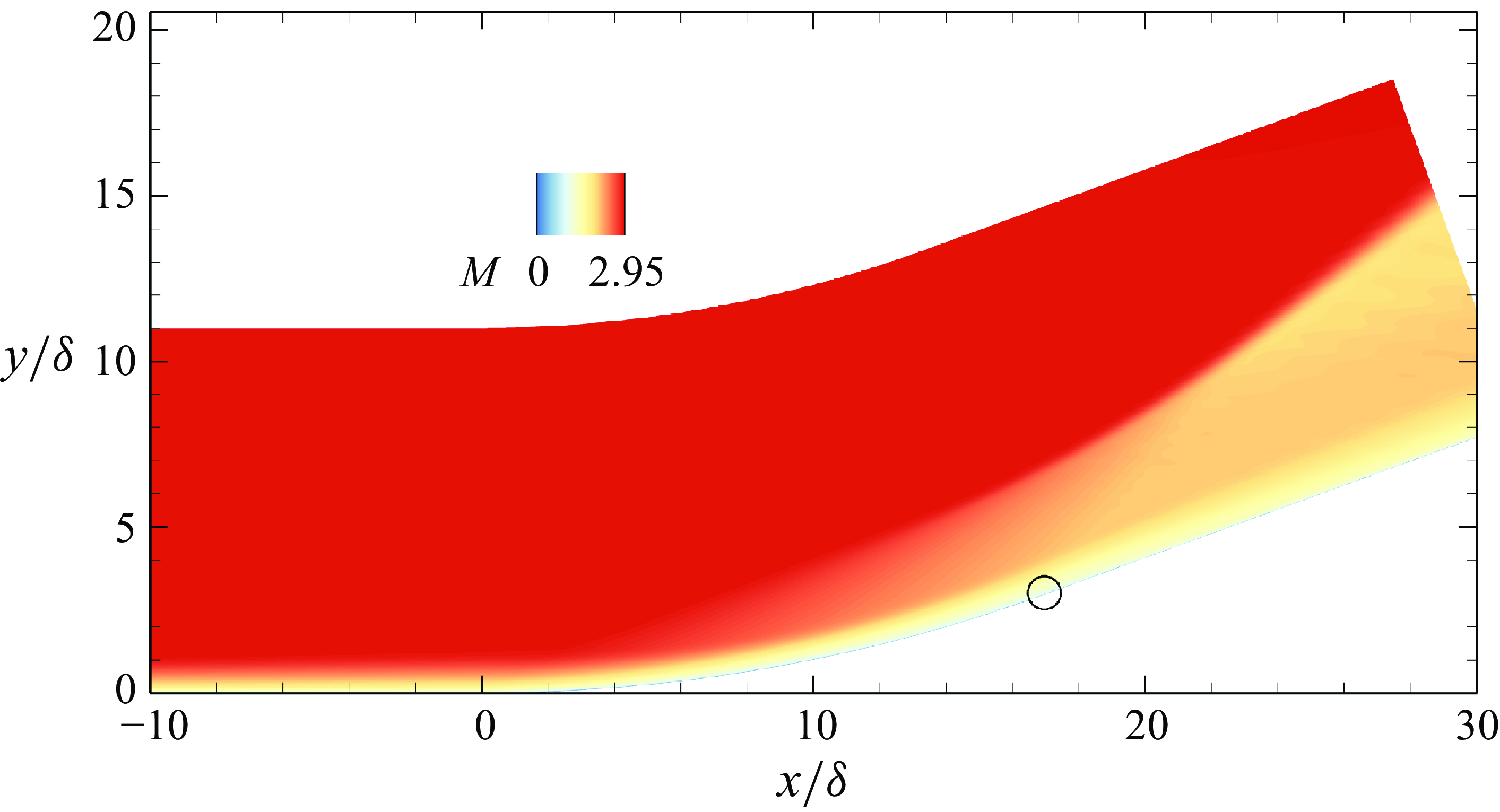
Figure 2. Contour of Mach number distribution at $ M_{\infty }=2.95$
,
$ M_{\infty }=2.95$
, $ Re_{\delta }=63\,500$
. The open circle indicates the end of the concave surface.
$ Re_{\delta }=63\,500$
. The open circle indicates the end of the concave surface.
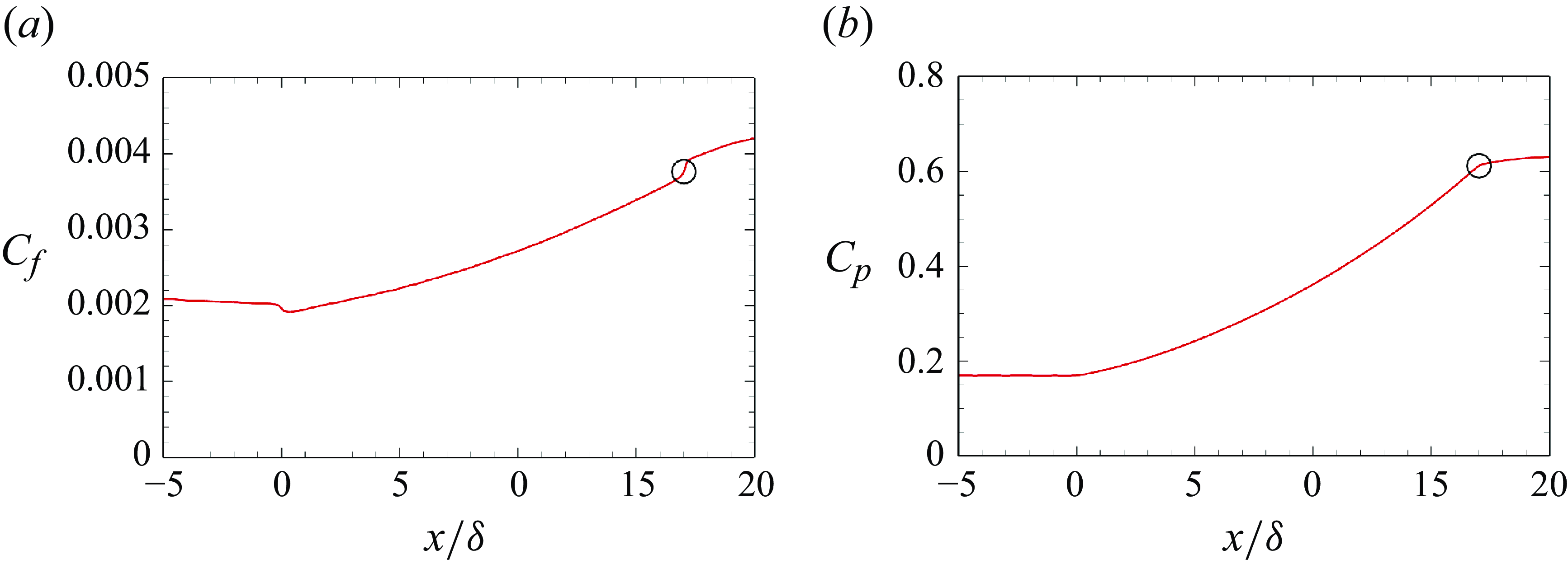
Figure 3. Distributions of ( $ a$
) the skin friction coefficient
$ a$
) the skin friction coefficient $ C_{f}$
, and (
$ C_{f}$
, and ( $ b$
) the wall pressure coefficient
$ b$
) the wall pressure coefficient $ C_{p}$
, at
$ C_{p}$
, at $ r=50\delta$
and
$ r=50\delta$
and $ \varphi =20^\circ$
. Open circles indicate the end of the concave region.
$ \varphi =20^\circ$
. Open circles indicate the end of the concave region.
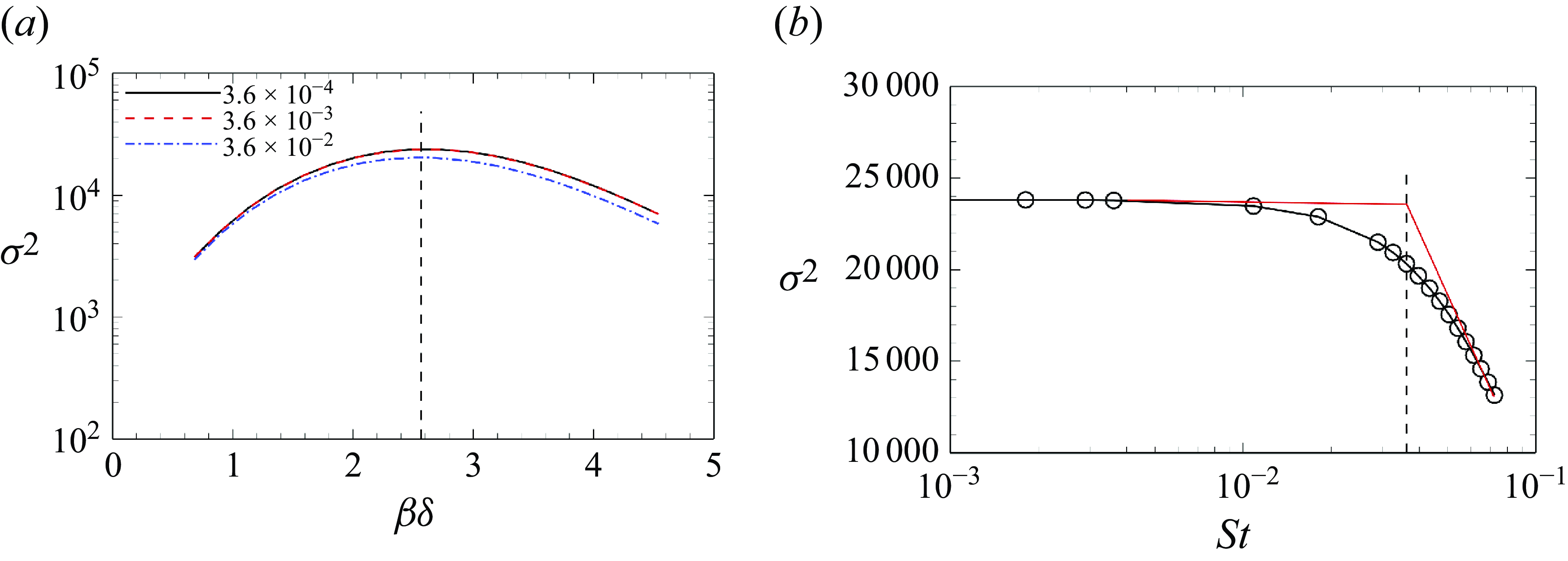
Figure 4. ( $ a$
) Optimal gains as a function of the spanwise wavenumber
$ a$
) Optimal gains as a function of the spanwise wavenumber $ \beta \delta$
at frequencies
$ \beta \delta$
at frequencies $ St=3.6\times {10}^{-4}, 3.6\times {10}^{-3}, 3.6\times {10}^{-2}$
. (
$ St=3.6\times {10}^{-4}, 3.6\times {10}^{-3}, 3.6\times {10}^{-2}$
. ( $ b$
) Optimal gains at
$ b$
) Optimal gains at $ \beta \delta=2.6$
over a range of frequencies. The black dashed line in (
$ \beta \delta=2.6$
over a range of frequencies. The black dashed line in ( $ a$
) means local maxima, while in (
$ a$
) means local maxima, while in ( $ b$
) it denotes the approximate cut-off frequency
$ b$
) it denotes the approximate cut-off frequency $ St =0.036$
. The red dashed lines indicate the cut-off frequency.
$ St =0.036$
. The red dashed lines indicate the cut-off frequency.
Resolvent analysis is then performed to study responses of the linear dynamic system (3.5) to upstream forcings, utilising the LES-computed mean flow as the base flow (Touber & Sandham Reference Touber and Sandham2009). The eddy viscosity $ {\mu }_{t}$
in the LES base flow is computed from
$ {\mu }_{t}$
in the LES base flow is computed from
 \begin{equation} {\mu }_{t}={C}_{\mu }\rho \frac {{k}^{2}}{\epsilon }, \end{equation}
where $ {C}_{\mu }=0.09$
,
$ {C}_{\mu }=0.09$
, $ \rho$
is the averaged density, and
$ \rho$
is the averaged density, and $ \epsilon$
is the rate of dissipation of turbulent kinetic energy (Pope Reference Pope2001). The turbulent kinetic energy
$ \epsilon$
is the rate of dissipation of turbulent kinetic energy (Pope Reference Pope2001). The turbulent kinetic energy $ k$
is defined as
$ k$
is defined as $ k=({1}/{2})\times (\langle u^{\prime\prime} u^{\prime\prime}\rangle + \langle v^{\prime\prime} v^{\prime\prime}\rangle + \langle w^{\prime\prime} w^{\prime\prime}\rangle )$
, where
$ k=({1}/{2})\times (\langle u^{\prime\prime} u^{\prime\prime}\rangle + \langle v^{\prime\prime} v^{\prime\prime}\rangle + \langle w^{\prime\prime} w^{\prime\prime}\rangle )$
, where $ \langle u^{\prime\prime} u^{\prime\prime}\rangle$
,
$ \langle u^{\prime\prime} u^{\prime\prime}\rangle$
, $ \langle v^{\prime\prime} v^{\prime\prime}\rangle$
and
$ \langle v^{\prime\prime} v^{\prime\prime}\rangle$
and $ \langle w^{\prime\prime} w^{\prime\prime}\rangle$
are the Reynolds stress components. The forcing station is set to
$ \langle w^{\prime\prime} w^{\prime\prime}\rangle$
are the Reynolds stress components. The forcing station is set to $ x=-10\delta$
. It should be noted that the optimal response is insensitive to the forcing location (see Appendix B).
$ x=-10\delta$
. It should be noted that the optimal response is insensitive to the forcing location (see Appendix B).
Figure 4( $ a$
) compares optimal gains at three frequencies
$ a$
) compares optimal gains at three frequencies $ St=3.6\times {10}^{-4}, 3.6\times {10}^{-3}, 3.6\times {10}^{-2}$
over a range of spanwise wavenumbers
$ St=3.6\times {10}^{-4}, 3.6\times {10}^{-3}, 3.6\times {10}^{-2}$
over a range of spanwise wavenumbers $ \beta \delta$
. Here, the frequency is defined as
$ \beta \delta$
. Here, the frequency is defined as $ St=f\delta /{u}_{\infty }$
. The overlap of optimal gains at
$ St=f\delta /{u}_{\infty }$
. The overlap of optimal gains at $ St=3.6\times {10}^{-4}$
and
$ St=3.6\times {10}^{-4}$
and $ St=3.6\times {10}^{-3}$
indicates that the optimal gains do not change significantly with further reductions in frequency. For
$ St=3.6\times {10}^{-3}$
indicates that the optimal gains do not change significantly with further reductions in frequency. For $ St=0.036$
, the optimal gains are slightly lower than those at the other two frequencies. Interestingly, all three optimal gain curves peak at the same spanwise wavenumber
$ St=0.036$
, the optimal gains are slightly lower than those at the other two frequencies. Interestingly, all three optimal gain curves peak at the same spanwise wavenumber $ \beta \delta = 2.6$
. Figure 4(
$ \beta \delta = 2.6$
. Figure 4( $ b$
) presents the optimal gains at the peak wavenumber
$ b$
) presents the optimal gains at the peak wavenumber $ \beta \delta = 2.6$
as a function of
$ \beta \delta = 2.6$
as a function of $ St$
. The distribution exhibits characteristics consistent with a first-order low-pass filter (Hunter Reference Hunter2001), demonstrating peak gains in the low-frequency regime
$ St$
. The distribution exhibits characteristics consistent with a first-order low-pass filter (Hunter Reference Hunter2001), demonstrating peak gains in the low-frequency regime $ St\lt 0.01$
. Beyond
$ St\lt 0.01$
. Beyond $ St=0.01$
, a gradual attenuation of optimal gain is observed, transitioning to a linear decay pattern when exceeding
$ St=0.01$
, a gradual attenuation of optimal gain is observed, transitioning to a linear decay pattern when exceeding $ St=0.04$
. An approximate cut-off frequency
$ St=0.04$
. An approximate cut-off frequency $ St=0.036$
is identified through the intersection of the
$ St=0.036$
is identified through the intersection of the $ St\lt 0.01$
and
$ St\lt 0.01$
and $ St\gt 0.04$
trends (marked in red) (Hunter Reference Hunter2001). This critical frequency denotes the threshold beyond which the linear system experiences a marked reduction in optimal gains. The selection of this specific cut-off frequency is further substantiated by SPOD analysis results, as detailed in § 4.2.2. The highest frequency considered in this study is
$ St\gt 0.04$
trends (marked in red) (Hunter Reference Hunter2001). This critical frequency denotes the threshold beyond which the linear system experiences a marked reduction in optimal gains. The selection of this specific cut-off frequency is further substantiated by SPOD analysis results, as detailed in § 4.2.2. The highest frequency considered in this study is $ St=0.072$
, which is at least one order lower than the characteristic frequency of TBLs, thereby satisfying the scale separation assumption.
$ St=0.072$
, which is at least one order lower than the characteristic frequency of TBLs, thereby satisfying the scale separation assumption.
Figure 5 shows the optimal forcing and corresponding response at $ St=0.036$
with spanwise wavenumber
$ St=0.036$
with spanwise wavenumber $ \beta \delta=2.6$
. The forcing corresponds to streamwise vortices, since the amplitudes of the wall-normal component
$ \beta \delta=2.6$
. The forcing corresponds to streamwise vortices, since the amplitudes of the wall-normal component $ | v^{\prime} |$
and the spanwise component
$ | v^{\prime} |$
and the spanwise component $ | w^{\prime} |$
are larger than that of the streamwise component
$ | w^{\prime} |$
are larger than that of the streamwise component $ | u^{\prime} |$
. The lift-up mechanism works to transform the streamwise vortices into streamwise streaks in the flow response (Abreu et al. Reference Abreu, Cavalieri, Schlatter, Vinuesa and Henningson2020; Hao et al. Reference Hao, Cao, Guo and Wen2023). The optimal response of
$ | u^{\prime} |$
. The lift-up mechanism works to transform the streamwise vortices into streamwise streaks in the flow response (Abreu et al. Reference Abreu, Cavalieri, Schlatter, Vinuesa and Henningson2020; Hao et al. Reference Hao, Cao, Guo and Wen2023). The optimal response of $ u^{\prime}$
displays streamwise streaks within and downstream of the concave region, while
$ u^{\prime}$
displays streamwise streaks within and downstream of the concave region, while $ w^{\prime}$
is characterised by streamwise counter-rotating vortices, as shown in figures 5(b,c). Upstream of the concave region, no apparent coherent structures can be observed. It is evident that concave curvature plays a vital role in forming and strengthening these coherent structures. In the concave region, the curved streamlines excite centrifugal effects. The secondary effect, known as the Görtler instability, becomes the dominant amplification mechanism in forming the streamwise vortices due to the large concave curvature 0.02 (Hoffmann et al. Reference Hoffmann, Muck and Bradshaw1985). Therefore, the streamwise counter-rotating vortices generated in the concave region are identified as Görtler vortices. In addition, these structures are similar in appearance, differing only in their streamwise lengths across the frequency band
$ w^{\prime}$
is characterised by streamwise counter-rotating vortices, as shown in figures 5(b,c). Upstream of the concave region, no apparent coherent structures can be observed. It is evident that concave curvature plays a vital role in forming and strengthening these coherent structures. In the concave region, the curved streamlines excite centrifugal effects. The secondary effect, known as the Görtler instability, becomes the dominant amplification mechanism in forming the streamwise vortices due to the large concave curvature 0.02 (Hoffmann et al. Reference Hoffmann, Muck and Bradshaw1985). Therefore, the streamwise counter-rotating vortices generated in the concave region are identified as Görtler vortices. In addition, these structures are similar in appearance, differing only in their streamwise lengths across the frequency band $St= 0.01{-}0.04$
, which strongly indicates that they are driven by the same physical mechanism.
$St= 0.01{-}0.04$
, which strongly indicates that they are driven by the same physical mechanism.
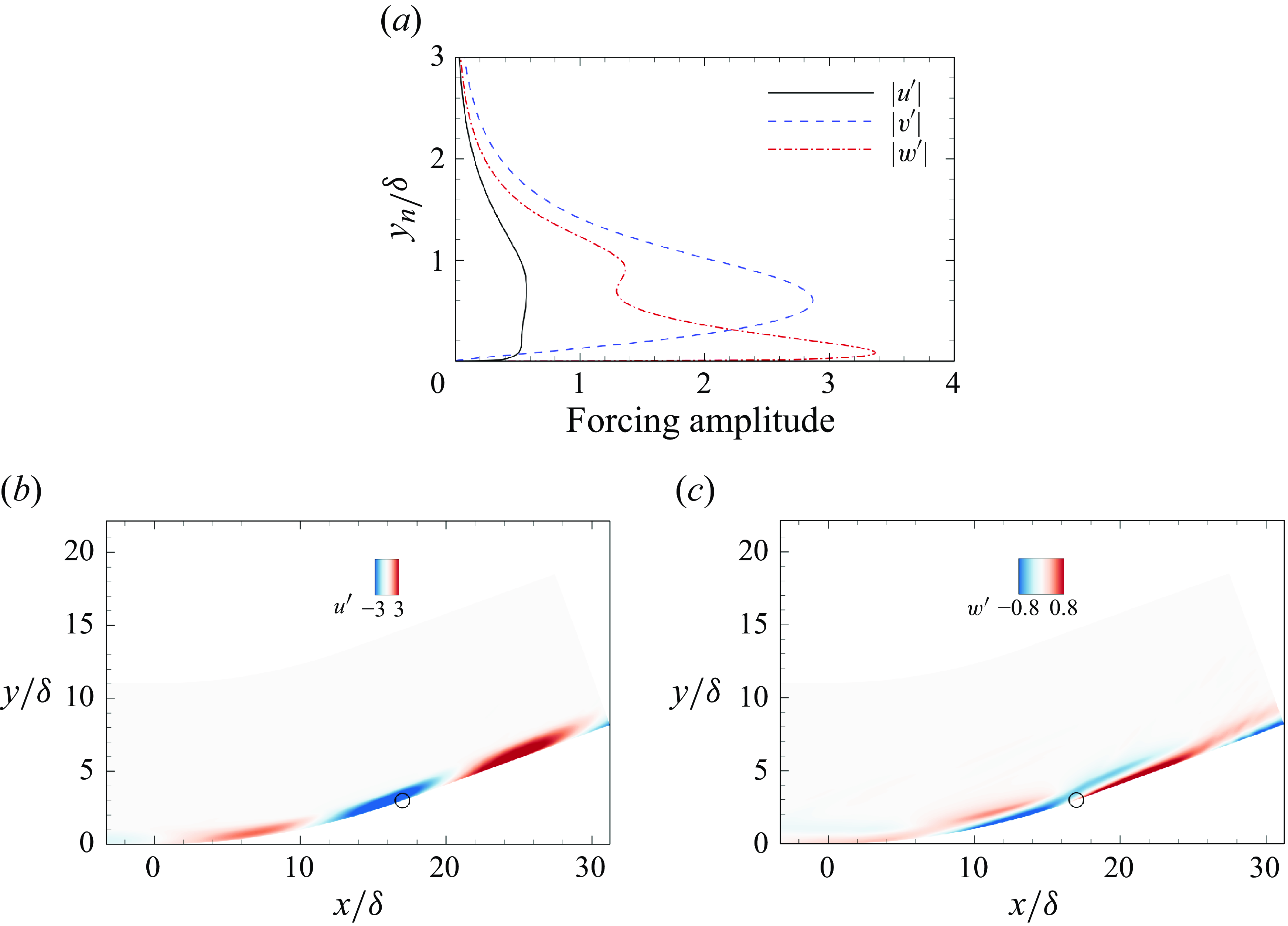
Figure 5. ( $ a$
) Amplitude of the optimal forcing. (b,c) Real parts of
$ a$
) Amplitude of the optimal forcing. (b,c) Real parts of $ u^{\prime}$
and
$ u^{\prime}$
and $ w^{\prime}$
of the optimal response at
$ w^{\prime}$
of the optimal response at $ St= 0.036$
and
$ St= 0.036$
and $ \beta \delta = 2.6$
. Open circles indictae the end of the concave region.
$ \beta \delta = 2.6$
. Open circles indictae the end of the concave region.
Furthermore, one can notice that the streamwise vortices are progressively strengthened in the concave region due to continuous centrifugal effects, resulting in a more pronounced $ u^{\prime}$
and
$ u^{\prime}$
and $ w^{\prime}$
in the latter half of the concave surface, as shown in figures 5(b,c). The three-dimensional perturbation field of
$ w^{\prime}$
in the latter half of the concave surface, as shown in figures 5(b,c). The three-dimensional perturbation field of $ u^{\prime}$
reconstructed using the optimal response at
$ u^{\prime}$
reconstructed using the optimal response at $ St=0.036$
and
$ St=0.036$
and $ \beta \delta =2.6$
is presented in figure 6. An intuitive comparison of the Görtler structures can be observed at different stations in the figure. At the beginning of the concave surface (station
$ \beta \delta =2.6$
is presented in figure 6. An intuitive comparison of the Görtler structures can be observed at different stations in the figure. At the beginning of the concave surface (station $ \varphi =0^{\circ }$
), weak spanwise structures are visible. Downstream of this station, the Görtler structures begin to grow. By the end of the concave surface, both the size and strength of the Görtler structures are significantly enhanced compared to values upstream.
$ \varphi =0^{\circ }$
), weak spanwise structures are visible. Downstream of this station, the Görtler structures begin to grow. By the end of the concave surface, both the size and strength of the Görtler structures are significantly enhanced compared to values upstream.

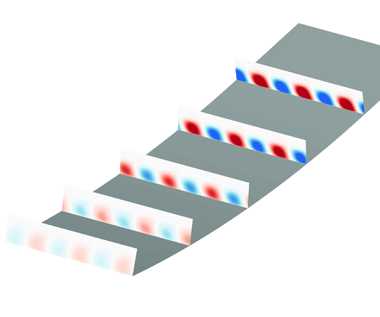
Figure 6. Three-dimensional reconstructed perturbation field of $ u^{\prime}$
using the optimal response at
$ u^{\prime}$
using the optimal response at $ St=0.036$
and
$ St=0.036$
and $ \beta \delta =2.6$
. The stations, from left to right, are
$ \beta \delta =2.6$
. The stations, from left to right, are $ \varphi =0^{\circ }$
,
$ \varphi =0^{\circ }$
, $ \varphi =5^{\circ }$
,
$ \varphi =5^{\circ }$
, $ \varphi =10^{\circ }$
,
$ \varphi =10^{\circ }$
, $ \varphi =15^{\circ }$
and
$ \varphi =15^{\circ }$
and $ \varphi =20^{\circ }$
, respectively.
$ \varphi =20^{\circ }$
, respectively.
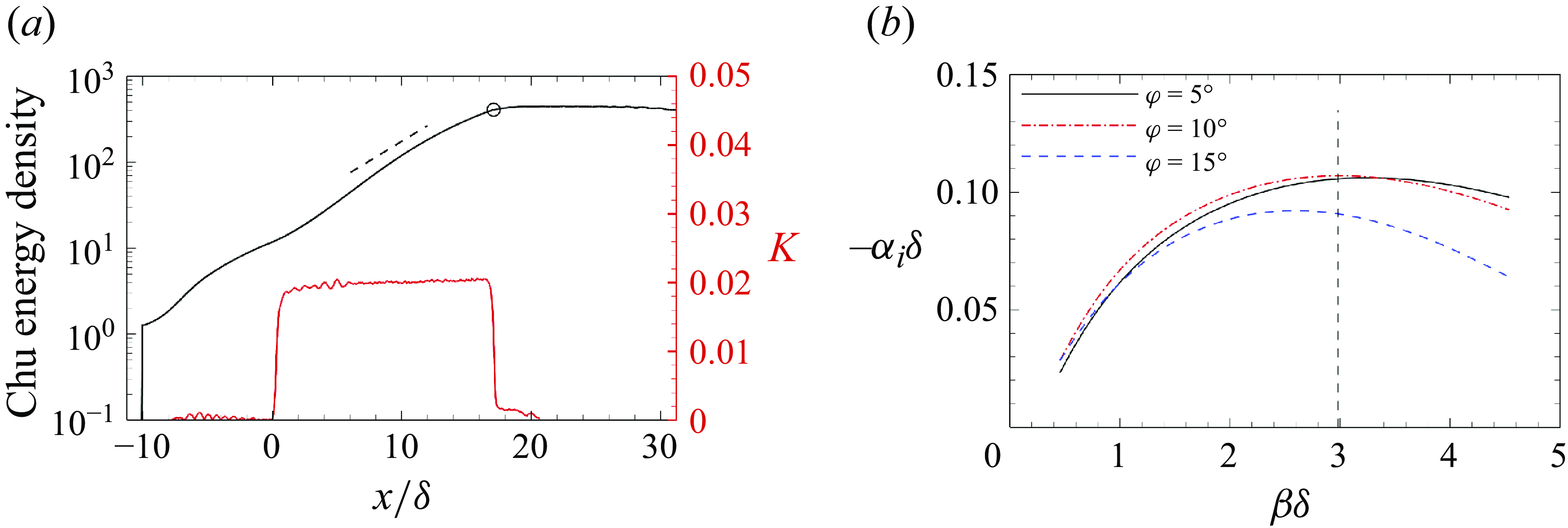
Figure 7. ( $ a$
) Distributions of the Chu energy density integrated in the wall-normal direction at
$ a$
) Distributions of the Chu energy density integrated in the wall-normal direction at $ St=0.036$
and
$ St=0.036$
and $ \beta \delta =2.6$
, and the curvature of the streamline passing through
$ \beta \delta =2.6$
, and the curvature of the streamline passing through $ (x_{0} , 0.3 \delta)$
. (
$ (x_{0} , 0.3 \delta)$
. ( $ b$
) The most unstable spatial growth rate at
$ b$
) The most unstable spatial growth rate at $ St=0.036$
from LSA as a function of spanwise wavenumbers
$ St=0.036$
from LSA as a function of spanwise wavenumbers $ \beta \delta$
at stations
$ \beta \delta$
at stations $ \varphi = 5^{\circ }$
,
$ \varphi = 5^{\circ }$
, $ \varphi = 10^{\circ }$
and
$ \varphi = 10^{\circ }$
and $ \varphi = 15^{\circ }$
. The black dashed line in (
$ \varphi = 15^{\circ }$
. The black dashed line in ( $ a$
) indicates the most unstable spatial growth rate predicted by LSA at station
$ a$
) indicates the most unstable spatial growth rate predicted by LSA at station $ \varphi = 10^{\circ }$
, while in (
$ \varphi = 10^{\circ }$
, while in ( $ b$
) it means the local maximum
$ b$
) it means the local maximum $ \beta \delta =2.98$
at
$ \beta \delta =2.98$
at $ \varphi = 10^{\circ }$
. The open circle indicates the end of the concave region.
$ \varphi = 10^{\circ }$
. The open circle indicates the end of the concave region.
To study the spatial energy growth rate of the optimal response in the concave region, the integrated wall-normal Chu energy density along the streamwise direction at $ St=0.036$
and
$ St=0.036$
and $ \beta \delta=2.6$
is presented in figure 7(
$ \beta \delta=2.6$
is presented in figure 7( $ a$
). The Chu energy density increases exponentially in the concave region, and peaks downstream of the region. The concave curvature
$ a$
). The Chu energy density increases exponentially in the concave region, and peaks downstream of the region. The concave curvature $ K$
of the streamline passing through
$ K$
of the streamline passing through $ (x_{0} , 0.3 \delta)$
stays constant in the concave region, indicating uniform centrifugal effects at different streamwise stations. Consequently, the energy of the coherent structures is exponentially amplified in the concave region under consistently strong centrifugal effects. The slope of the black dashed line is predicted by LSA at station
$ (x_{0} , 0.3 \delta)$
stays constant in the concave region, indicating uniform centrifugal effects at different streamwise stations. Consequently, the energy of the coherent structures is exponentially amplified in the concave region under consistently strong centrifugal effects. The slope of the black dashed line is predicted by LSA at station $ \varphi = 10^{\circ }$
at
$ \varphi = 10^{\circ }$
at $ St=0.036$
and
$ St=0.036$
and $ \beta \delta= 2.6$
. There is good agreement between the growth rate from LSA and resolvent analysis at the same station, which indicates that the energy growth is mainly attributed to the convective-type non-normality, i.e. the Görtler instability. Figure 7(
$ \beta \delta= 2.6$
. There is good agreement between the growth rate from LSA and resolvent analysis at the same station, which indicates that the energy growth is mainly attributed to the convective-type non-normality, i.e. the Görtler instability. Figure 7( $ b$
) depicts the most unstable spatial growth rates at
$ b$
) depicts the most unstable spatial growth rates at $ St=0.036$
predicted by LSA at three stations as functions of spanwise wavenumbers
$ St=0.036$
predicted by LSA at three stations as functions of spanwise wavenumbers $ \beta \delta$
. Although the peak wavenumbers of the three lines differ slightly, they are centred around
$ \beta \delta$
. Although the peak wavenumbers of the three lines differ slightly, they are centred around $ \beta \delta= 2.98$
. There is a small discrepancy between the peak wavenumbers predicted by LSA and resolvent analysis. This discrepancy is reasonable, as the wavenumber predicted by LSA is locally optimal, while the global optimal wavenumber from resolvent analysis may vary due to non-parallelism and non-modal effects (Hanifi, Schmid & Henningson Reference Hanifi, Schmid and Henningson1996; Tumin & Reshotko Reference Tumin and Reshotko2003). Figure 8 compares the wall-normal distributions of the amplitudes of
$ \beta \delta= 2.98$
. There is a small discrepancy between the peak wavenumbers predicted by LSA and resolvent analysis. This discrepancy is reasonable, as the wavenumber predicted by LSA is locally optimal, while the global optimal wavenumber from resolvent analysis may vary due to non-parallelism and non-modal effects (Hanifi, Schmid & Henningson Reference Hanifi, Schmid and Henningson1996; Tumin & Reshotko Reference Tumin and Reshotko2003). Figure 8 compares the wall-normal distributions of the amplitudes of $ u^{\prime}$
and
$ u^{\prime}$
and $ w^{\prime}$
obtained from two methods at the three stations
$ w^{\prime}$
obtained from two methods at the three stations $ \varphi = 5^{\circ }$
,
$ \varphi = 5^{\circ }$
, $ \varphi = 10^{\circ }$
and
$ \varphi = 10^{\circ }$
and $ \varphi = 15^{\circ }$
. Here,
$ \varphi = 15^{\circ }$
. Here, $ u^{\prime}$
peaks near the wall then decreases linearly, while
$ u^{\prime}$
peaks near the wall then decreases linearly, while $ w^{\prime}$
exhibits two peaks: one near the wall, and another near the edge of the TBL. The trends of
$ w^{\prime}$
exhibits two peaks: one near the wall, and another near the edge of the TBL. The trends of $ u^{\prime}$
and
$ u^{\prime}$
and $ w^{\prime}$
are almost the same at three streamwise stations of the two results, with minor differences in the location of the second peak of
$ w^{\prime}$
are almost the same at three streamwise stations of the two results, with minor differences in the location of the second peak of $ w^{\prime}$
and the wall-normal range of the large amplitude of
$ w^{\prime}$
and the wall-normal range of the large amplitude of $ u^{\prime}$
. It is confirmed that the most amplified disturbances in resolvent analysis are the Görtler vortices.
$ u^{\prime}$
. It is confirmed that the most amplified disturbances in resolvent analysis are the Görtler vortices.
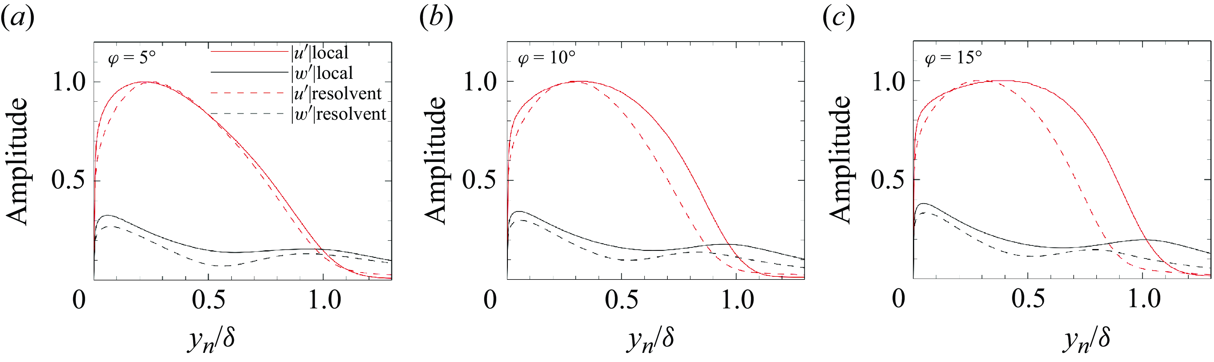
Figure 8. Comparisons of wall-normal distributions of streamwise velocity and spanwise velocity perturbations from LSA and resolvent analysis at stations ( $ a$
)
$ a$
) $ \varphi = 5^{\circ }$
, (
$ \varphi = 5^{\circ }$
, ( $ b$
)
$ b$
) $ \varphi = 10^{\circ }$
and (
$ \varphi = 10^{\circ }$
and ( $ c$
)
$ c$
) $ \varphi = 15^{\circ }$
, at
$ \varphi = 15^{\circ }$
, at $ St=0.036$
and
$ St=0.036$
and $ \beta \delta= 2.6$
. Distributions are normalised by their respective maximum streamwise velocity perturbation amplitudes.
$ \beta \delta= 2.6$
. Distributions are normalised by their respective maximum streamwise velocity perturbation amplitudes.
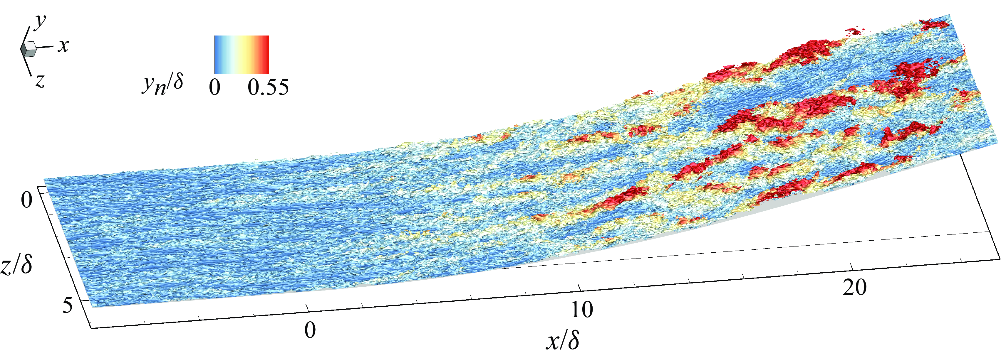
Figure 9. Iso-surface of streamwise velocity $ u/{u}_{\infty }=0.55$
, coloured by wall-normal distance.
$ u/{u}_{\infty }=0.55$
, coloured by wall-normal distance.
4.2. Validation of predicted coherent structures
4.2.1. Amplification of turbulence intensity
Figure 9 illustrates the instantaneous iso-surface of streamwise velocity $ u/{u}_{\infty }=0.55$
, coloured by wall-normal distance. On the flat plate, only a few near-wall vortices are visible, whereas large-scale vortices are prominent in the concave region. The centrifugal effects in this region continue to drive low-momentum flow outwards, thereby enhancing the momentum exchange between low- and high-momentum flows (Wang et al. Reference Wang, Wang, Sun, Yang, Zhao and Hu2019). Additionally, it is noteworthy that the spanwise scale of the vortices in the concave region gradually increases.
$ u/{u}_{\infty }=0.55$
, coloured by wall-normal distance. On the flat plate, only a few near-wall vortices are visible, whereas large-scale vortices are prominent in the concave region. The centrifugal effects in this region continue to drive low-momentum flow outwards, thereby enhancing the momentum exchange between low- and high-momentum flows (Wang et al. Reference Wang, Wang, Sun, Yang, Zhao and Hu2019). Additionally, it is noteworthy that the spanwise scale of the vortices in the concave region gradually increases.
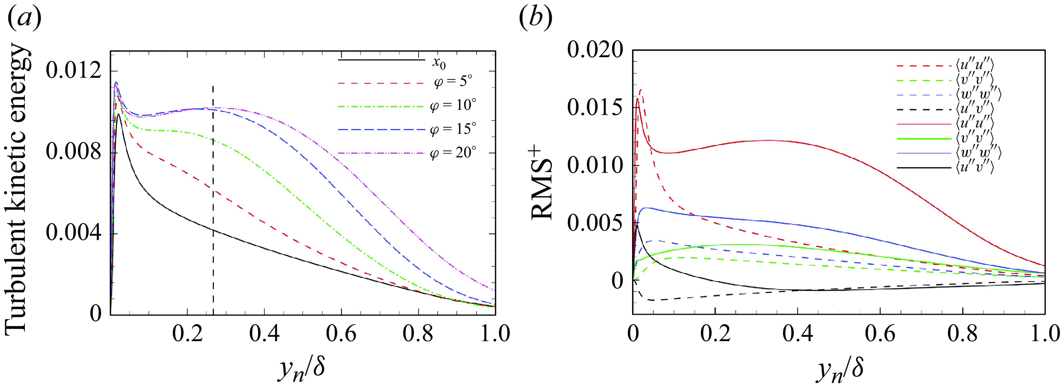
Figure 10. Wall-normal distributions of ( $ a$
) turbulent kinetic energy
$ a$
) turbulent kinetic energy $ k$
, (
$ k$
, ( $ b$
) root mean square values RMS
$ b$
) root mean square values RMS $ ^{+}$
, normalised by
$ ^{+}$
, normalised by $ {u}_{\infty }^{2}$
. The black dashed line in (
$ {u}_{\infty }^{2}$
. The black dashed line in ( $ a$
) denotes
$ a$
) denotes $ y{}_{n}/\delta =0.26$
. In (b), the dashed and solid lines correspond to the reference station (
$ y{}_{n}/\delta =0.26$
. In (b), the dashed and solid lines correspond to the reference station ( $x_0$
) and the end of the concave region (
$x_0$
) and the end of the concave region ( $\varphi=20^{\circ}$
), respectively.
$\varphi=20^{\circ}$
), respectively.
Figure 10( $ a$
) shows the wall-normal distributions of the turbulent kinetic energy
$ a$
) shows the wall-normal distributions of the turbulent kinetic energy $ k$
at the reference station
$ k$
at the reference station $ x_{0}$
and the four different turning angle stations in the concave surface. At station
$ x_{0}$
and the four different turning angle stations in the concave surface. At station $ x_{0}$
,
$ x_{0}$
, $ k$
peaks at a near-wall location, primarily due to high- and low-speed streaks. In the concave region, the inner part of
$ k$
peaks at a near-wall location, primarily due to high- and low-speed streaks. In the concave region, the inner part of $ k$
is slightly enhanced, while the outer part experiences significant amplification. Continuous centrifugal effects amplify turbulent fluctuations, leading to a noticeable increase in the outer part of
$ k$
is slightly enhanced, while the outer part experiences significant amplification. Continuous centrifugal effects amplify turbulent fluctuations, leading to a noticeable increase in the outer part of $ k$
across various stations. A second peak of
$ k$
across various stations. A second peak of $ k$
, associated with the large-scale vortices shown in figure 9, occurs at approximately
$ k$
, associated with the large-scale vortices shown in figure 9, occurs at approximately $ y{}_{n}/\delta =0.26$
at the end of the concave surface.
$ y{}_{n}/\delta =0.26$
at the end of the concave surface.
Figure 10( $ b$
) compares wall-normal distributions of Reynolds stress components
$ b$
) compares wall-normal distributions of Reynolds stress components $ \langle u^{\prime\prime} u^{\prime\prime}\rangle$
,
$ \langle u^{\prime\prime} u^{\prime\prime}\rangle$
, $ \langle v^{\prime\prime} v^{\prime\prime} \rangle$
,
$ \langle v^{\prime\prime} v^{\prime\prime} \rangle$
, $ \langle w^{\prime\prime} w^{\prime\prime}\rangle$
and
$ \langle w^{\prime\prime} w^{\prime\prime}\rangle$
and $ \langle u^{\prime\prime} v^{\prime\prime}\rangle$
at the reference station
$ \langle u^{\prime\prime} v^{\prime\prime}\rangle$
at the reference station $ x_{0}$
and the end of the concave surface
$ x_{0}$
and the end of the concave surface $ \varphi =20^{\circ }$
. Compared to the undisturbed TBL, all Reynolds stress components show significant changes at
$ \varphi =20^{\circ }$
. Compared to the undisturbed TBL, all Reynolds stress components show significant changes at $ \varphi =20^{\circ }$
. The trends of
$ \varphi =20^{\circ }$
. The trends of $ \langle v^{\prime\prime} v^{\prime\prime}\rangle$
and
$ \langle v^{\prime\prime} v^{\prime\prime}\rangle$
and $ \langle w^{\prime\prime} w^{\prime\prime}\rangle$
are the same as those at station
$ \langle w^{\prime\prime} w^{\prime\prime}\rangle$
are the same as those at station $ x_{0}$
, although their amplitudes are increased. In contrast,
$ x_{0}$
, although their amplitudes are increased. In contrast, $ \langle u^{\prime\prime} u^{\prime\prime}\rangle$
exhibits a notable discrepancy in the outer layer. After a decrease from the inner peak,
$ \langle u^{\prime\prime} u^{\prime\prime}\rangle$
exhibits a notable discrepancy in the outer layer. After a decrease from the inner peak, $ \langle u^{\prime\prime} u^{\prime\prime}\rangle$
increases again to form a secondary peak influencing
$ \langle u^{\prime\prime} u^{\prime\prime}\rangle$
increases again to form a secondary peak influencing $ y{}_{n}/\delta =0.1{-}0.6$
. The outer peak of
$ y{}_{n}/\delta =0.1{-}0.6$
. The outer peak of $ \langle u^{\prime\prime} u^{\prime\prime}\rangle$
is associated with the large-scale structures highlighted in figure 9. Moreover, the peak of
$ \langle u^{\prime\prime} u^{\prime\prime}\rangle$
is associated with the large-scale structures highlighted in figure 9. Moreover, the peak of $ k$
in the outer layer at the station
$ k$
in the outer layer at the station $ \varphi =20^{\circ }$
is mainly contributed by the streamwise component
$ \varphi =20^{\circ }$
is mainly contributed by the streamwise component $ \langle u^{\prime\prime} u^{\prime\prime}\rangle$
. Notably, the near-wall part of the component
$ \langle u^{\prime\prime} u^{\prime\prime}\rangle$
. Notably, the near-wall part of the component $ \langle u^{\prime\prime} v^{\prime\prime}\rangle$
changes sign at station
$ \langle u^{\prime\prime} v^{\prime\prime}\rangle$
changes sign at station $ \varphi =20^{\circ }$
, which is attributed to mathematical contaminations between longitudinal and wall-normal velocities in Cartesian coordinates (Wu et al. Reference Wu, Liang and Zhao2019). Similar distributions in
$ \varphi =20^{\circ }$
, which is attributed to mathematical contaminations between longitudinal and wall-normal velocities in Cartesian coordinates (Wu et al. Reference Wu, Liang and Zhao2019). Similar distributions in $ k$
and Reynolds stress components were also discussed by Wu et al. (Reference Wu, Liang and Zhao2019) and Sun et al. (Reference Sun, Sandham and Hu2019).
$ k$
and Reynolds stress components were also discussed by Wu et al. (Reference Wu, Liang and Zhao2019) and Sun et al. (Reference Sun, Sandham and Hu2019).
4.2.2. Modal analysis
The POD analysis is performed on $ y$
–
$ y$
– $z$
slices in the concave region to study spatial structures of large-scale vortices. Here, the entire state vector
$z$
slices in the concave region to study spatial structures of large-scale vortices. Here, the entire state vector $ {q}^{\prime }= [ \rho ^{\prime},u^{\prime},v^{\prime},w^{\prime},T^{\prime} ]$
is used, combined with the Chu energy norm (Chu Reference Chu1965). The fluctuation variables are normalised with the freestream parameters. The convergence analysis of POD modes is discussed in Appendix C.
$ {q}^{\prime }= [ \rho ^{\prime},u^{\prime},v^{\prime},w^{\prime},T^{\prime} ]$
is used, combined with the Chu energy norm (Chu Reference Chu1965). The fluctuation variables are normalised with the freestream parameters. The convergence analysis of POD modes is discussed in Appendix C.
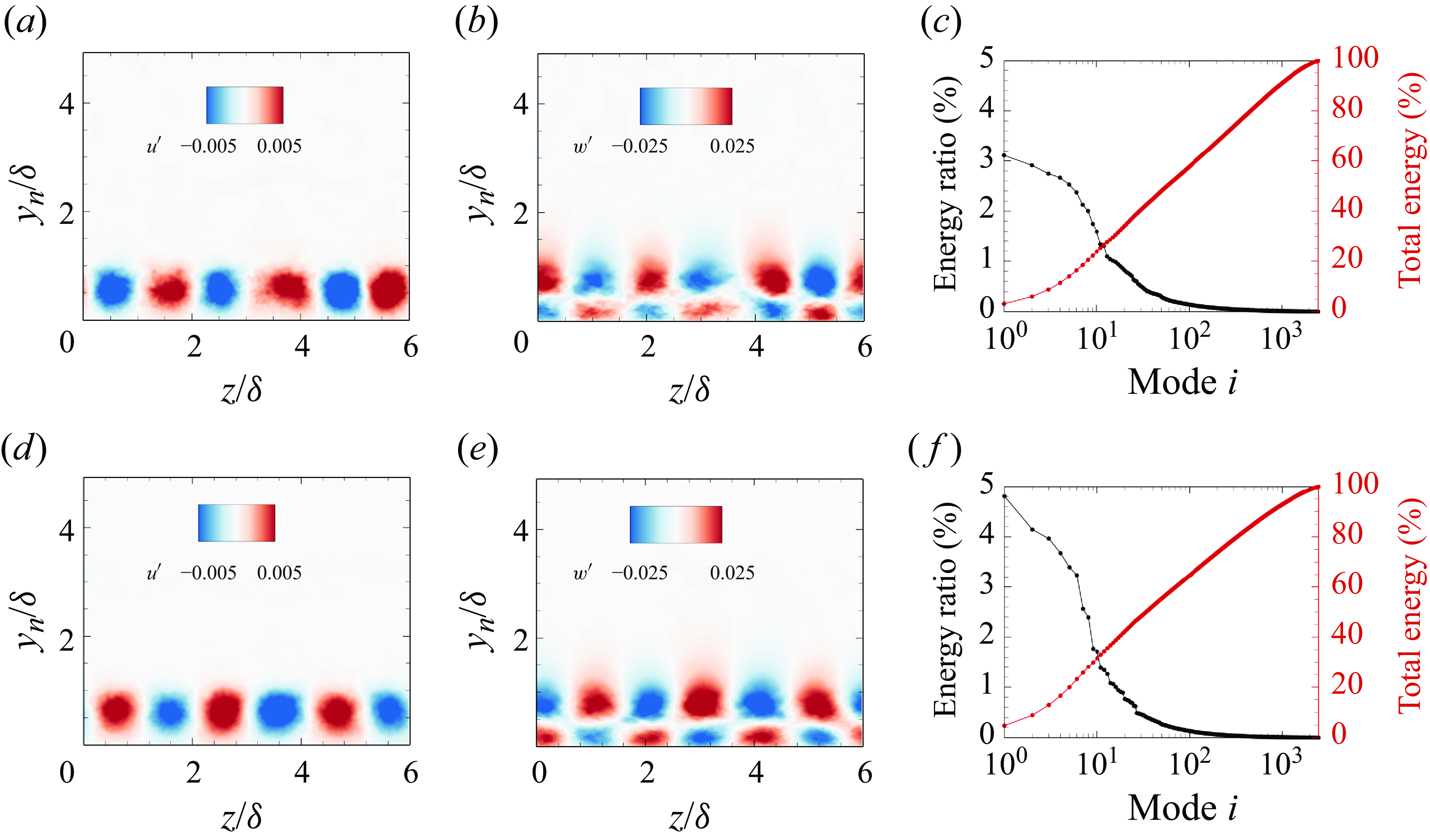
Figure 11. Leading POD modes of ( $ a$
)
$ a$
) $ u^{\prime}$
, (
$ u^{\prime}$
, ( $ b$
)
$ b$
) $ w^{\prime}$
at station
$ w^{\prime}$
at station $ \varphi =10^{\circ }$
, and (
$ \varphi =10^{\circ }$
, and ( $ d$
)
$ d$
) $ u^{\prime}$
, (
$ u^{\prime}$
, ( $ e$
)
$ e$
) $ w^{\prime}$
at station
$ w^{\prime}$
at station $ \varphi =20^{\circ }$
. (c,f) The mode energy distributions at the two stations.
$ \varphi =20^{\circ }$
. (c,f) The mode energy distributions at the two stations.
Figure 11 demonstrates the components $ u^{\prime}$
and
$ u^{\prime}$
and $ w^{\prime}$
of the leading POD modes at stations
$ w^{\prime}$
of the leading POD modes at stations $ \varphi =10^{\circ }$
and
$ \varphi =10^{\circ }$
and $ \varphi =20^{\circ }$
, as well as mode energy distributions. Three pairs of spanwise structures can be observed in figures 11(a,b) at station
$ \varphi =20^{\circ }$
, as well as mode energy distributions. Three pairs of spanwise structures can be observed in figures 11(a,b) at station $ \varphi =10^{\circ }$
. The component
$ \varphi =10^{\circ }$
. The component $ u^{\prime}$
is characterised by streamwise streaks, and
$ u^{\prime}$
is characterised by streamwise streaks, and $ w^{\prime}$
features streamwise counter-rotating vortices. The most energetic spatial structures closely resemble the coherent structures predicted by resolvent analysis in figure 6. At station
$ w^{\prime}$
features streamwise counter-rotating vortices. The most energetic spatial structures closely resemble the coherent structures predicted by resolvent analysis in figure 6. At station $ \varphi =20^{\circ }$
, the spatial structures behave analogously to those at
$ \varphi =20^{\circ }$
, the spatial structures behave analogously to those at $ \varphi =10^{\circ }$
. The spanwise scale at both stations is approximately
$ \varphi =10^{\circ }$
. The spanwise scale at both stations is approximately $ {\lambda }_{z}=2\delta$
, leading to three pairs of spanwise structures. Regarding the energy distribution, the energy ratio of the leading POD mode at both stations is minimal, falling below
$ {\lambda }_{z}=2\delta$
, leading to three pairs of spanwise structures. Regarding the energy distribution, the energy ratio of the leading POD mode at both stations is minimal, falling below $ 5\, \%$
. Most of the energy is captured by numerous high-order modes. In addition, the sum of eigenvalues at station
$ 5\, \%$
. Most of the energy is captured by numerous high-order modes. In addition, the sum of eigenvalues at station $ \varphi =20^{\circ }$
is 0.57, compared to 0.24 at station
$ \varphi =20^{\circ }$
is 0.57, compared to 0.24 at station $ \varphi =10^{\circ }$
. The rise of total energy agrees well with the turbulence amplification caused by the centrifugal effects discussed in § 4.2.1.
$ \varphi =10^{\circ }$
. The rise of total energy agrees well with the turbulence amplification caused by the centrifugal effects discussed in § 4.2.1.
Nevertheless, it should be emphasised that conventional POD modes may conflate dynamically distinct phenomena when different flow features exhibit comparable energy content at disparate frequencies (Towne et al. Reference Towne, Schmidt and Colonius2018; Mendez, Balabane & Buchlin Reference Mendez, Balabane and Buchlin2019). This multi-modal coupling characteristic fundamentally limits the temporal discrimination capability of energy-based decomposition methods. To overcome this limitation, we use the frequency-resolved method named SPOD to investigate the spatial–temporal features of the coherent structures induced by the concave surface.
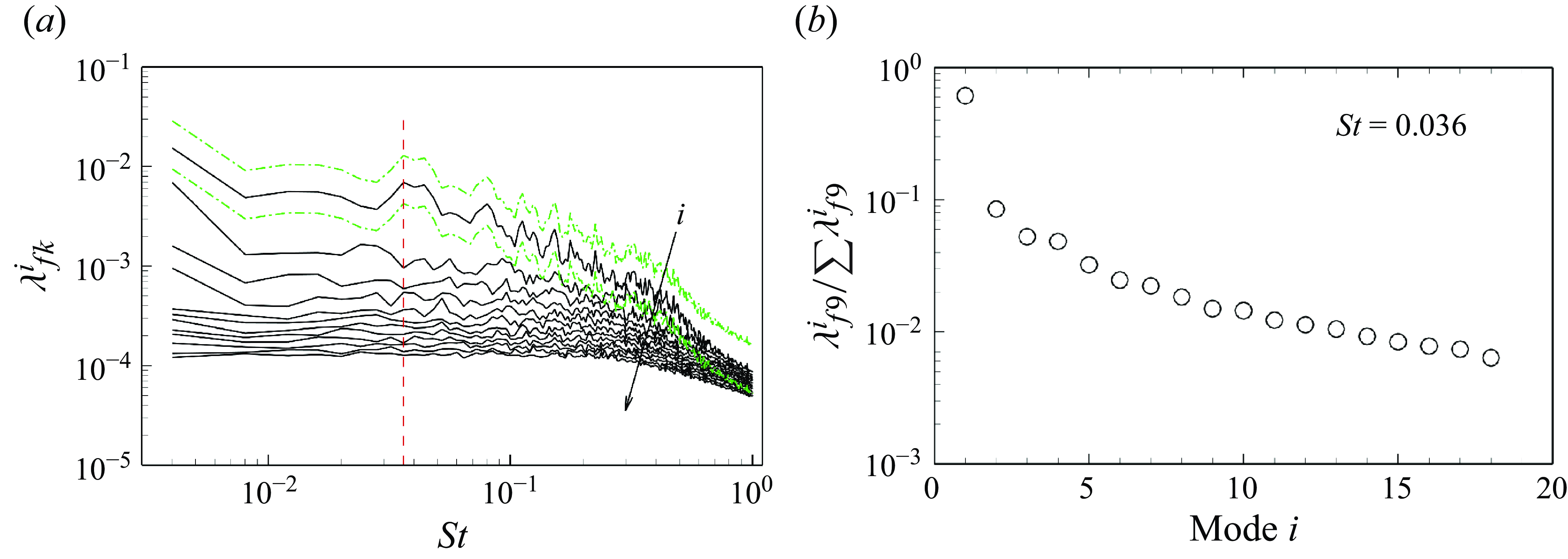
Figure 12. ( $ a$
) Normalised SPOD eigenvalues as functions of
$ a$
) Normalised SPOD eigenvalues as functions of $ St$
. The 99
$ St$
. The 99 $ \, \%$
confidence bounds for the leading mode are indicated by the green dash-dotted lines. The red dashed line marks the local maximum
$ \, \%$
confidence bounds for the leading mode are indicated by the green dash-dotted lines. The red dashed line marks the local maximum $ St=0.036$
. (
$ St=0.036$
. ( $ b$
) Normalised SPOD eigenvalues at
$ b$
) Normalised SPOD eigenvalues at $ St=0.036$
.
$ St=0.036$
.
The SPOD is first performed on the spanwise mid-plane using a temporal segment $ 249.1 \delta /{u}_{\infty }$
. Welch’s method (Welch Reference Welch1967) with 50
$ 249.1 \delta /{u}_{\infty }$
. Welch’s method (Welch Reference Welch1967) with 50 $ \, \%$
overlap combining a Hamming window is employed to minimise spectral leakage. Notably, the specific choice of window function shows negligible impact on the results, as equivalent frequency spectra are obtained when using a Hann window. A convergence analysis of the SPOD modes is provided in Appendix C. The spectrum is presented in figure 12(
$ \, \%$
overlap combining a Hamming window is employed to minimise spectral leakage. Notably, the specific choice of window function shows negligible impact on the results, as equivalent frequency spectra are obtained when using a Hann window. A convergence analysis of the SPOD modes is provided in Appendix C. The spectrum is presented in figure 12( $ a$
), where the 99
$ a$
), where the 99 $ \, \%$
bounds indicate the variance of the leading mode. A characteristic frequency
$ \, \%$
bounds indicate the variance of the leading mode. A characteristic frequency $ St=0.036$
of the leading mode is identified. Figure 12(
$ St=0.036$
of the leading mode is identified. Figure 12( $ b$
) compares the normalised eigenvalues at
$ b$
) compares the normalised eigenvalues at $ St=0.036$
. A low-rank feature is observed, with the optimal SPOD mode containing 65
$ St=0.036$
. A low-rank feature is observed, with the optimal SPOD mode containing 65 $ \, \%$
of the total flow energy – significantly more energetic than the other suboptimal modes at this frequency.
$ \, \%$
of the total flow energy – significantly more energetic than the other suboptimal modes at this frequency.
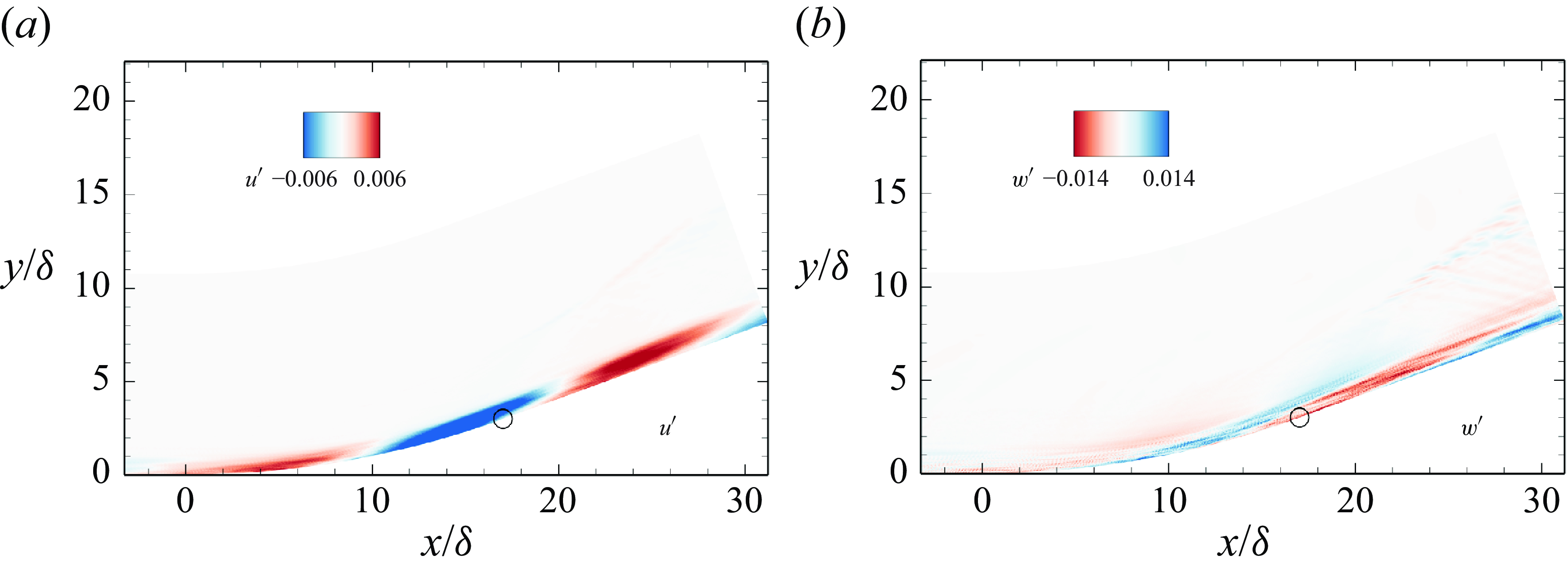
Figure 13. Real parts of ( $ a$
)
$ a$
) $ u^{\prime}$
and (
$ u^{\prime}$
and ( $ b$
)
$ b$
) $ w^{\prime}$
of the optimal SPOD mode at
$ w^{\prime}$
of the optimal SPOD mode at $ St=0.036$
. Open circles indicate the end of the concave surface.
$ St=0.036$
. Open circles indicate the end of the concave surface.
Figures 13(a,b) display the real parts of $ u^{\prime}$
and
$ u^{\prime}$
and $ w^{\prime}$
of the optimal SPOD mode at
$ w^{\prime}$
of the optimal SPOD mode at $ St=0.036$
. In response to upstream turbulent forcings, streamwise streaks of
$ St=0.036$
. In response to upstream turbulent forcings, streamwise streaks of $ u^{\prime}$
and
$ u^{\prime}$
and $ w^{\prime}$
are observed within and downstream of the concave region. Notably, both
$ w^{\prime}$
are observed within and downstream of the concave region. Notably, both $ u^{\prime}$
and
$ u^{\prime}$
and $ w^{\prime}$
exhibit stronger intensities in the latter half of the concave surface, indicating an enhancement of the coherent structures in this region. This enhancement process and the coherent structures resemble those obtained from resolvent analysis at the same frequency, as shown in figure 5. To quantitatively compare the leading SPOD mode with the optimal resolvent modes, we calculate the projection coefficient
$ w^{\prime}$
exhibit stronger intensities in the latter half of the concave surface, indicating an enhancement of the coherent structures in this region. This enhancement process and the coherent structures resemble those obtained from resolvent analysis at the same frequency, as shown in figure 5. To quantitatively compare the leading SPOD mode with the optimal resolvent modes, we calculate the projection coefficient $ \gamma$
using the equation
$ \gamma$
using the equation
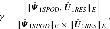 \begin{equation} \gamma =\frac {\left | \| \hat{\boldsymbol{\Psi}}_{1\textit{SPOD}}, \hat{\boldsymbol{U}}_{1\textit{RES}}\|_{E} \right |}{ \| \hat{\boldsymbol{\Psi }}_{1\textit{SPOD}}\|_{E} \times \|\hat{\boldsymbol{U}}_{1\textit{RES}}\|_{E} }, \end{equation}
where $ \hat{\boldsymbol{\Psi}}_{1\textit{SPOD}}$
represents the leading SPOD mode, while
$ \hat{\boldsymbol{\Psi}}_{1\textit{SPOD}}$
represents the leading SPOD mode, while $ \hat{\boldsymbol{U}}_{1\textit{RES}}$
denotes the optimal resolvent modes over several spanwise wavenumbers. The notation
$ \hat{\boldsymbol{U}}_{1\textit{RES}}$
denotes the optimal resolvent modes over several spanwise wavenumbers. The notation $ {\| \cdot \|}_{E}$
denotes the Chu norm (Chu Reference Chu1965). A value
$ {\| \cdot \|}_{E}$
denotes the Chu norm (Chu Reference Chu1965). A value $ \gamma = 0$
indicates orthogonality between the two modes, while
$ \gamma = 0$
indicates orthogonality between the two modes, while $ \gamma = 1$
signifies perfect alignment (Abreu et al. Reference Abreu, Cavalieri, Schlatter, Vinuesa and Henningson2020; Fan et al. Reference Fan, Kozul, Li and Sandberg2024). Notably, the leading SPOD mode
$ \gamma = 1$
signifies perfect alignment (Abreu et al. Reference Abreu, Cavalieri, Schlatter, Vinuesa and Henningson2020; Fan et al. Reference Fan, Kozul, Li and Sandberg2024). Notably, the leading SPOD mode $ \hat{\boldsymbol{\Psi }}_{1\textit{SPOD}}(x,y)$
combines Fourier modes at various wavelengths implicitly, while
$ \hat{\boldsymbol{\Psi }}_{1\textit{SPOD}}(x,y)$
combines Fourier modes at various wavelengths implicitly, while $ \hat{\boldsymbol{U}}_{1\textit{RES}}(x,y)$
represents structures at a single specified wavelength explicitly. Hence this projection quantifies the structural similarity between the coherent structures captured by the leading SPOD mode and those predicted by resolvent analysis, while simultaneously identifying the dominant wavelength in the SPOD mode through the peak
$ \hat{\boldsymbol{U}}_{1\textit{RES}}(x,y)$
represents structures at a single specified wavelength explicitly. Hence this projection quantifies the structural similarity between the coherent structures captured by the leading SPOD mode and those predicted by resolvent analysis, while simultaneously identifying the dominant wavelength in the SPOD mode through the peak $ \gamma (\beta \delta )$
. Cura et al. (Reference Cura, Hanifi, Cavalieri and Weiss2024) also successfully made the projection between the leading SPOD mode obtained using particle image velocimetry data in a planar and resolvent modes to investigate the low-frequency dynamics of turbulent separation bubbles. Figure 14 shows the projection coefficients
$ \gamma (\beta \delta )$
. Cura et al. (Reference Cura, Hanifi, Cavalieri and Weiss2024) also successfully made the projection between the leading SPOD mode obtained using particle image velocimetry data in a planar and resolvent modes to investigate the low-frequency dynamics of turbulent separation bubbles. Figure 14 shows the projection coefficients $ \gamma$
between the optimal SPOD mode and the predicted resolvent modes at
$ \gamma$
between the optimal SPOD mode and the predicted resolvent modes at $ St = 0.036$
over various spanwise wavenumbers. The peak alignment,
$ St = 0.036$
over various spanwise wavenumbers. The peak alignment, $ \gamma = 0.94$
, is very close to 1, indicating an almost perfect match between the two modes. The optimal response is strongly associated with observed streamwise streaks in SPOD. Moreover, the coefficient reaches its maximum at spanwise wavenumber
$ \gamma = 0.94$
, is very close to 1, indicating an almost perfect match between the two modes. The optimal response is strongly associated with observed streamwise streaks in SPOD. Moreover, the coefficient reaches its maximum at spanwise wavenumber $ \beta \delta = 2.95$
, which corresponds well with the optimal wavenumber predicted by resolvent analysis and the most unstable wavenumber identified by LSA.
$ \beta \delta = 2.95$
, which corresponds well with the optimal wavenumber predicted by resolvent analysis and the most unstable wavenumber identified by LSA.
Hence there is a strong correlation between the optimal SPOD mode and the optimal response. The relation between SPOD and resolvent analysis has been discussed by Towne et al. (Reference Towne, Schmidt and Colonius2018), Schmidt et al. (Reference Schmidt, Towne, Rigas, Colonius and Brès2018) and Abreu et al. (Reference Abreu, Cavalieri, Schlatter, Vinuesa and Henningson2020). When forcings are unit-variance white noise, SPOD is equivalent to resolvent analysis. In real turbulent flows, biased and nonlinear forcings (Morra et al. Reference Morra, Nogueira, Cavalieri and Henningson2021) result in differences between SPOD and resolvent modes. However, a close match between the leading SPOD mode and the optimal resolvent mode can be achieved when the resolvent operator identifies a dominant amplification mechanism (Abreu et al. Reference Abreu, Cavalieri, Schlatter, Vinuesa and Henningson2020). In such cases, the leading SPOD modes and the optimal resolvent modes are insensitive to the correlation of nonlinear forcings $ E(\,\,\hat {\boldsymbol{\!\!f}}\,\hat {\boldsymbol{\!\!f}}^{*})$
, where
$ E(\,\,\hat {\boldsymbol{\!\!f}}\,\hat {\boldsymbol{\!\!f}}^{*})$
, where $ E(\cdot )$
is the expectation operator. Therefore, the similarity of mode shapes and the high alignment between the leading SPOD mode and the optimal response suggest that the same physical mechanism, namely the centrifugal effects, dominates the most energetic coherent structures. In other words, the Görtler instability primarily amplifies upstream forcings and forms the Görtler vortices.
$ E(\cdot )$
is the expectation operator. Therefore, the similarity of mode shapes and the high alignment between the leading SPOD mode and the optimal response suggest that the same physical mechanism, namely the centrifugal effects, dominates the most energetic coherent structures. In other words, the Görtler instability primarily amplifies upstream forcings and forms the Görtler vortices.
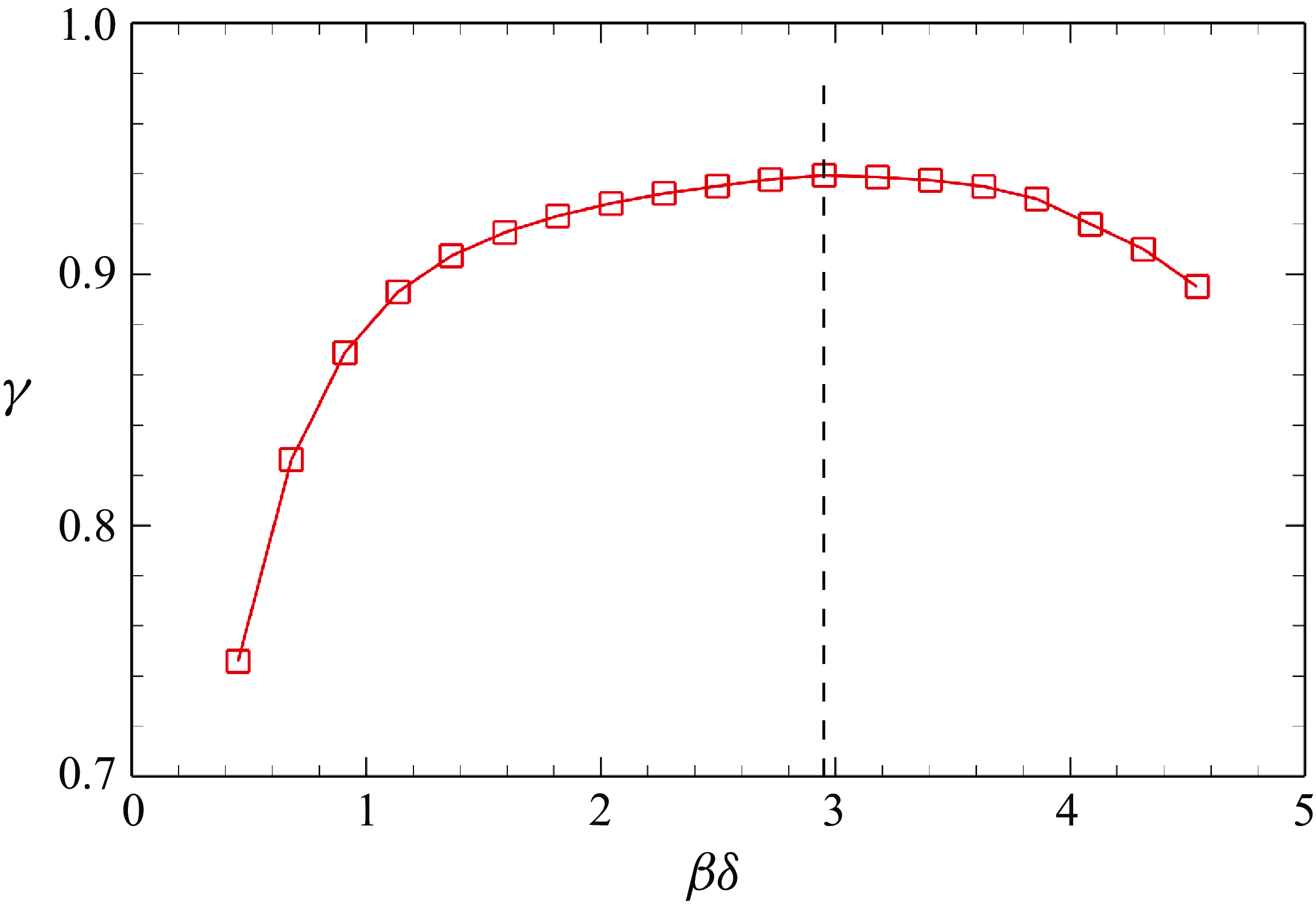
Figure 14. Projection coefficients $ {\gamma }$
between the optimal SPOD mode and resolvent modes over varying spanwise wavenumber at
$ {\gamma }$
between the optimal SPOD mode and resolvent modes over varying spanwise wavenumber at $ St=0.036$
. The black dashed line indicates local maximum
$ St=0.036$
. The black dashed line indicates local maximum $ \beta \delta =2.95$
.
$ \beta \delta =2.95$
.
Furthermore, the flow statistics characterised at the peak frequency $ St=0.036$
in the streamwise direction make it reasonable to choose the frequency as the approximate cut-off frequency. The optimal SPOD modes within the frequency band
$ St=0.036$
in the streamwise direction make it reasonable to choose the frequency as the approximate cut-off frequency. The optimal SPOD modes within the frequency band $St= 0.01{-}0.04$
also resemble those obtained from resolvent analysis, with the SPOD mode being more energetic at
$St= 0.01{-}0.04$
also resemble those obtained from resolvent analysis, with the SPOD mode being more energetic at $ St=0.036$
due to coloured forcings. Consequently, resolvent analysis successfully captures flow structures in the streamwise direction, and serves as an effective tool for studying Görtler instability. The next step is to compare the spanwise scales from both methods, and investigate the formation process of Görtler vortices in the spanwise direction under the influence of centrifugal effects.
$ St=0.036$
due to coloured forcings. Consequently, resolvent analysis successfully captures flow structures in the streamwise direction, and serves as an effective tool for studying Görtler instability. The next step is to compare the spanwise scales from both methods, and investigate the formation process of Görtler vortices in the spanwise direction under the influence of centrifugal effects.
The SPOD is then conducted on $ y$
–
$ y$
– $ z$
slices in the concave region using the sine-taper SPOD (Yeung & Schmidt Reference Yeung and Schmidt2024). The peak frequencies of the first SPOD modes at different stations do not consistently align with
$ z$
slices in the concave region using the sine-taper SPOD (Yeung & Schmidt Reference Yeung and Schmidt2024). The peak frequencies of the first SPOD modes at different stations do not consistently align with $ St=0.036$
, as shown in table 1. This variation is expected because Görtler vortices are active over a frequency band
$ St=0.036$
, as shown in table 1. This variation is expected because Görtler vortices are active over a frequency band $St= 0.01{-}0.04$
, as discussed in § 4.1. The coherent structures and spanwise scales of the leading SPOD modes within this frequency band are quite similar. Here, we focus on the coherent structures at
$St= 0.01{-}0.04$
, as discussed in § 4.1. The coherent structures and spanwise scales of the leading SPOD modes within this frequency band are quite similar. Here, we focus on the coherent structures at $ St= 0.036$
to quantitatively assess their spanwise scales and structures. Figure 15 depicts the real parts of
$ St= 0.036$
to quantitatively assess their spanwise scales and structures. Figure 15 depicts the real parts of $ u^{\prime}$
and
$ u^{\prime}$
and $ w^{\prime}$
of the leading SPOD modes at three stations
$ w^{\prime}$
of the leading SPOD modes at three stations $ \varphi = {10}^{\circ }$
,
$ \varphi = {10}^{\circ }$
, $\varphi ={15}^{\circ }$
and
$\varphi ={15}^{\circ }$
and $\varphi ={20}^{\circ }$
, at
$\varphi ={20}^{\circ }$
, at $ St=0.036$
. At station
$ St=0.036$
. At station $ \varphi = {5}^{\circ }$
, the Görtler vortices are not fully developed (not shown here). The Görtler vortices emerge at stations
$ \varphi = {5}^{\circ }$
, the Görtler vortices are not fully developed (not shown here). The Görtler vortices emerge at stations $\varphi ={10}^{\circ }$
, where
$\varphi ={10}^{\circ }$
, where $ u^{\prime}$
displays pairs of streamwise streaks, and
$ u^{\prime}$
displays pairs of streamwise streaks, and $ w^{\prime}$
shows pairs of streamwise counter-rotating vortices. Downstream of this station, the coherent structures at station
$ w^{\prime}$
shows pairs of streamwise counter-rotating vortices. Downstream of this station, the coherent structures at station $\varphi ={15}^{\circ }$
and
$\varphi ={15}^{\circ }$
and $\varphi ={20}^{\circ }$
remain unchanged.
$\varphi ={20}^{\circ }$
remain unchanged.
Table 1. The peak frequencies at different stations of the leading SPOD modes.
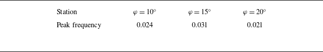
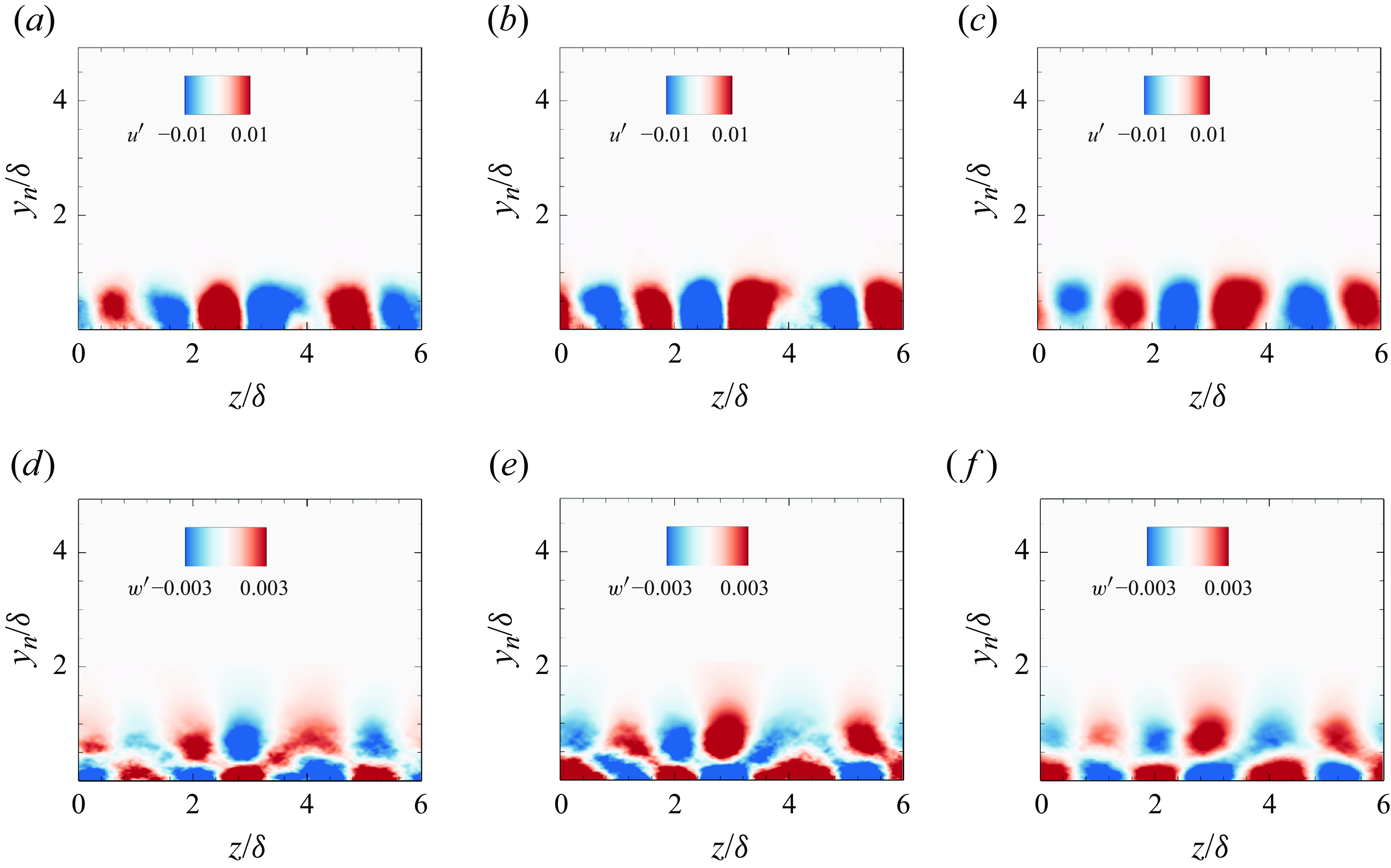
Figure 15. Real parts of the optimal SPOD modes of $ u^{\prime}$
and
$ u^{\prime}$
and $ w^{\prime}$
at stations (a,d)
$ w^{\prime}$
at stations (a,d) $ \varphi = {10}^{\circ }$
, (b,e)
$ \varphi = {10}^{\circ }$
, (b,e) $ \varphi = {15}^{\circ }$
and (c,f)
$ \varphi = {15}^{\circ }$
and (c,f) $ \varphi = {20}^{\circ }$
, at
$ \varphi = {20}^{\circ }$
, at $ St=0.036$
.
$ St=0.036$
.
The spanwise scales of the Görtler vortices at these stations are approximately consistent, averaging approximately $ 2\delta$
. However, it is noteworthy that some vortices exceed
$ 2\delta$
. However, it is noteworthy that some vortices exceed $ 2\delta$
, while others are smaller, suggesting that the spanwise structures exhibit a degree of irregularity. This phenomenon is expected and related to nonlinear effects in turbulent flows. The predicted optimal spanwise wavelength
$ 2\delta$
, while others are smaller, suggesting that the spanwise structures exhibit a degree of irregularity. This phenomenon is expected and related to nonlinear effects in turbulent flows. The predicted optimal spanwise wavelength $ 2.4\delta$
by resolvent analysis is slightly larger than the
$ 2.4\delta$
by resolvent analysis is slightly larger than the $ 2\delta$
captured by the optimal SPOD mode. The minor discrepancy is attributed to upstream biased forcings. In resolvent analysis, upstream forcings are treated as unbiased, while real turbulent fluctuations are biased and coloured (Morra et al. Reference Morra, Nogueira, Cavalieri and Henningson2021). These coloured forcings tend to concentrate most of the energy in near-wall streaks and very-large-scale motions, explaining the expected
$ 2\delta$
captured by the optimal SPOD mode. The minor discrepancy is attributed to upstream biased forcings. In resolvent analysis, upstream forcings are treated as unbiased, while real turbulent fluctuations are biased and coloured (Morra et al. Reference Morra, Nogueira, Cavalieri and Henningson2021). These coloured forcings tend to concentrate most of the energy in near-wall streaks and very-large-scale motions, explaining the expected $ 2\delta$
patterns observed in the optimal SPOD mode. Overall, resolvent analysis effectively models the Görtler vortices in terms of spatial–temporal features.
$ 2\delta$
patterns observed in the optimal SPOD mode. Overall, resolvent analysis effectively models the Görtler vortices in terms of spatial–temporal features.
Unsteady motions of the Görtler vortices can be recovered using the first five SPOD modes within the frequency band $ St=0.01{-}0.04$
, which contain at least 50
$ St=0.01{-}0.04$
, which contain at least 50 $ \, \%$
of total energy at a given frequency (Nekkanti & Schmidt Reference Nekkanti and Schmidt2021; Yeung & Schmidt Reference Yeung and Schmidt2024). The choice of this frequency band is based on two factors: first, the cut-off frequency band discussed in § 4.1, and second, the dynamic modes strongly related to Görtler vortices at frequencies 0.0115, 0.0172 and 0.0223 found by Tong et al. (Reference Tong, Li, Duan and Yu2017). The unsteady spanwise motions of the Görtler vortices can be observed from time series (see the supplementary movie). The large-scale Görtler vortices undergo a series of unsteady behaviours, including lateral wandering, merging into larger vortices, and splitting into several smaller ones. These merging and splitting behaviours are related to the spanwise motions of vortices, with varying lateral velocities leading to interactions between vortex pairs. No preferred vortex locations are found from the reconstructed data, consistent with experimental findings (Barlow & Johnston Reference Barlow and Johnston1988a
,Reference Barlow and Johnston
b
; Schuelein & Trofimov Reference Schuelein and Trofimov2011).
$ \, \%$
of total energy at a given frequency (Nekkanti & Schmidt Reference Nekkanti and Schmidt2021; Yeung & Schmidt Reference Yeung and Schmidt2024). The choice of this frequency band is based on two factors: first, the cut-off frequency band discussed in § 4.1, and second, the dynamic modes strongly related to Görtler vortices at frequencies 0.0115, 0.0172 and 0.0223 found by Tong et al. (Reference Tong, Li, Duan and Yu2017). The unsteady spanwise motions of the Görtler vortices can be observed from time series (see the supplementary movie). The large-scale Görtler vortices undergo a series of unsteady behaviours, including lateral wandering, merging into larger vortices, and splitting into several smaller ones. These merging and splitting behaviours are related to the spanwise motions of vortices, with varying lateral velocities leading to interactions between vortex pairs. No preferred vortex locations are found from the reconstructed data, consistent with experimental findings (Barlow & Johnston Reference Barlow and Johnston1988a
,Reference Barlow and Johnston
b
; Schuelein & Trofimov Reference Schuelein and Trofimov2011).
5. Scaling of Görtler vortices
The alignment between the leading SPOD modes obtained from the LES dataset and resolvent modes based on the LES base flow confirms the validity of resolvent analysis for capturing Görtler vortices dynamics. While resolvent analysis with LES base flows achieves high fidelity, a systematic parametric investigation of the spanwise scale sensitivity to geometric and freestream parameters – across multiple configurations – would be computationally prohibitive if relying solely on LES-based resolvent analysis. To balance accuracy and practicality, we adopt RANS-based resolvent analysis for the parametric study in this section. To validate this approach, § 5.1 first compares RANS-based resolvent analysis results against the LES-based methodology, demonstrating quantitative agreement in mode structures and optimal gains. Subsequent subsections then leverage RANS-based analysis to examine parameter dependencies, with the validated methodology ensuring robustness of the conclusions.
5.1. The RANS-based resolvent analysis
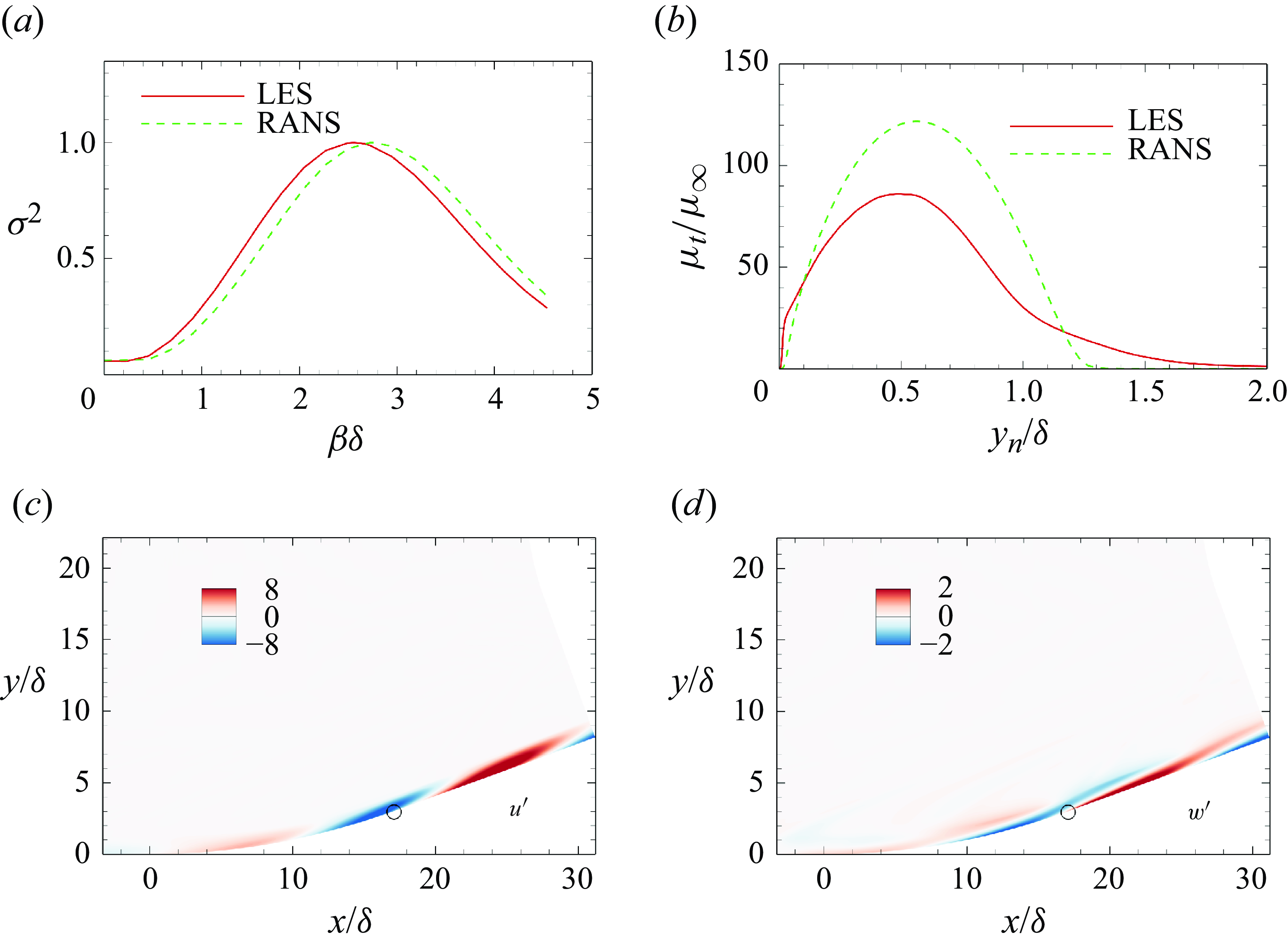
Figure 16. (a) Normalised optimal gains based on LES and RANS base flows at $ St=0.036$
. (
$ St=0.036$
. ( $ b$
) Distributions of
$ b$
) Distributions of $ \mu _{t}$
at the reference station
$ \mu _{t}$
at the reference station $ x_{0}$
from LES and RANS base flows. (c,d) Real parts of
$ x_{0}$
from LES and RANS base flows. (c,d) Real parts of $ u^{\prime}$
and
$ u^{\prime}$
and $ w^{\prime}$
based on the RANS base flow at
$ w^{\prime}$
based on the RANS base flow at $ St=0.036$
and
$ St=0.036$
and $ \beta \delta =2.75$
. Open circles indicate the ends of the concave surface.
$ \beta \delta =2.75$
. Open circles indicate the ends of the concave surface.
Figure 16( $ a$
) compares the normalised optimal gains from LES- and RANS-based resolvent analysis at
$ a$
) compares the normalised optimal gains from LES- and RANS-based resolvent analysis at $ St=0.036$
. The RANS results exhibit a marginally higher peak wavenumber
$ St=0.036$
. The RANS results exhibit a marginally higher peak wavenumber $ \beta \delta =2.75$
compared to the LES-based value
$ \beta \delta =2.75$
compared to the LES-based value $ \beta \delta =2.6$
. This minor shift aligns with expectations from eddy viscosity
$ \beta \delta =2.6$
. This minor shift aligns with expectations from eddy viscosity $ {\mu }_{t}$
discrepancies between the methodologies, as discussed in a flat plate case by Cossu, Pujals & Depardon (Reference Cossu, Pujals and Depardon2009). Figure 16(
$ {\mu }_{t}$
discrepancies between the methodologies, as discussed in a flat plate case by Cossu, Pujals & Depardon (Reference Cossu, Pujals and Depardon2009). Figure 16( $ b$
) further reveals that both LES and RANS profiles share similar
$ b$
) further reveals that both LES and RANS profiles share similar $ {\mu }_{t}$
trends, peaking near
$ {\mu }_{t}$
trends, peaking near $ y_{n}/\delta =0.5$
, though the RANS-based
$ y_{n}/\delta =0.5$
, though the RANS-based $ {\mu }_{t}$
magnitude exceeds the LES value by approximately 50
$ {\mu }_{t}$
magnitude exceeds the LES value by approximately 50 $ \, \%$
. Despite these differences, the optimal responses of
$ \, \%$
. Despite these differences, the optimal responses of $ u^{\prime}$
and
$ u^{\prime}$
and $ w^{\prime}$
at
$ w^{\prime}$
at $ \beta \delta =2.75$
shown in figures 16(c,d) resemble the optimal responses in figures 5(b,c) and the leading SPOD mode in figures 13(a,b) at the same frequency
$ \beta \delta =2.75$
shown in figures 16(c,d) resemble the optimal responses in figures 5(b,c) and the leading SPOD mode in figures 13(a,b) at the same frequency $ St=0.036$
. Quantitative validation is further supported by a peak projection coefficient
$ St=0.036$
. Quantitative validation is further supported by a peak projection coefficient $ \gamma =0.9$
between the leading SPOD mode and the RANS-based optimal response at
$ \gamma =0.9$
between the leading SPOD mode and the RANS-based optimal response at $ \beta \delta =2.95$
. These results collectively indicate that the most amplified dynamics revealed by resolvent analysis is insensitive to the relatively small differences in the
$ \beta \delta =2.95$
. These results collectively indicate that the most amplified dynamics revealed by resolvent analysis is insensitive to the relatively small differences in the $ {\mu }_{t}$
distributions (Cossu et al. Reference Cossu, Pujals and Depardon2009; Fan et al. Reference Fan, Kozul, Li and Sandberg2024). Pickering et al. (Reference Pickering, Rigas, Schmidt, Sipp and Colonius2021) demonstrated that the classical eddy-viscosity models (e.g. RANS) behave identically to an optimal eddy-viscosity model in aligning the most energetic mode. This agreement also underscores that the predicted most energetic response and scales derived from RANS-based
$ {\mu }_{t}$
distributions (Cossu et al. Reference Cossu, Pujals and Depardon2009; Fan et al. Reference Fan, Kozul, Li and Sandberg2024). Pickering et al. (Reference Pickering, Rigas, Schmidt, Sipp and Colonius2021) demonstrated that the classical eddy-viscosity models (e.g. RANS) behave identically to an optimal eddy-viscosity model in aligning the most energetic mode. This agreement also underscores that the predicted most energetic response and scales derived from RANS-based $ \mu _{t}$
, despite inherent modelling uncertainties, retain physical fidelity and provide reliable predictions. Consequently, the subsequent parametric investigations in this study employ RANS-based flows, balancing computational efficiency with demonstrated predictive fidelity.
$ \mu _{t}$
, despite inherent modelling uncertainties, retain physical fidelity and provide reliable predictions. Consequently, the subsequent parametric investigations in this study employ RANS-based flows, balancing computational efficiency with demonstrated predictive fidelity.
5.2. Geometric parameters
Two geometric parameters are considered: the total turning angle $ \varphi$
, and the curvature radius
$ \varphi$
, and the curvature radius $ r$
. It should be noted that the frequency is set to
$ r$
. It should be noted that the frequency is set to $ St=0.036$
, which is a representative frequency for Görtler vortices.
$ St=0.036$
, which is a representative frequency for Görtler vortices.
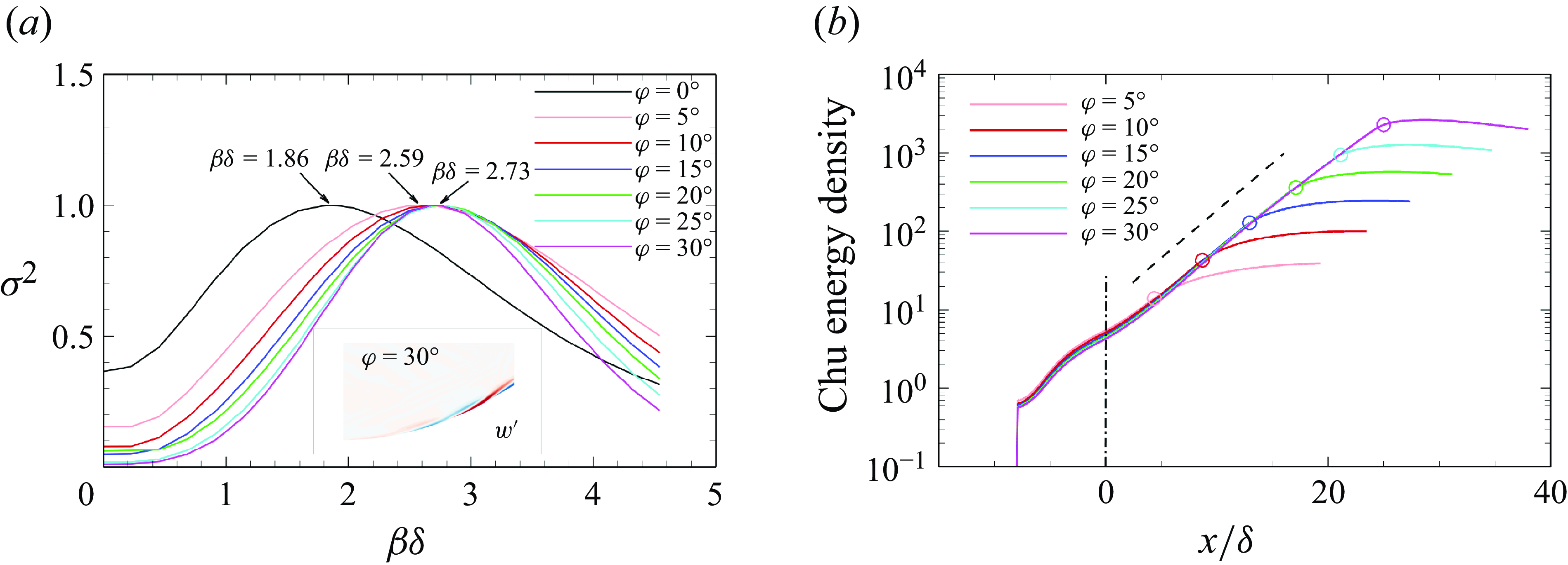
Figure 17. ( $ a$
) Normalised optimal gains at different turning angles as functions of spanwise wavenumbers
$ a$
) Normalised optimal gains at different turning angles as functions of spanwise wavenumbers $ \beta \delta$
. (
$ \beta \delta$
. ( $ b$
) Distributions of integrated Chu energy density along the wall-normal direction at different turning angles at their respectively optimal wavenumber. The inset in (
$ b$
) Distributions of integrated Chu energy density along the wall-normal direction at different turning angles at their respectively optimal wavenumber. The inset in ( $ a$
) represents the real part of
$ a$
) represents the real part of $ w^{\prime}$
for the optimal response in the case
$ w^{\prime}$
for the optimal response in the case $ \varphi =30^{\circ }$
, while the arrows indicate local maxima for different cases. The black dash-dotted line in (
$ \varphi =30^{\circ }$
, while the arrows indicate local maxima for different cases. The black dash-dotted line in ( $ b$
) indicates the beginning of the concave surfaces, the black dashed line represents the predicted increasing trend by LSA in figure 7(
$ b$
) indicates the beginning of the concave surfaces, the black dashed line represents the predicted increasing trend by LSA in figure 7( $ a$
), and the open circles denote the ends of the concave surfaces.
$ a$
), and the open circles denote the ends of the concave surfaces.
Figure 17( $ a$
) shows the distributions of the optimal gains at different turning angles for a constant curvature radius
$ a$
) shows the distributions of the optimal gains at different turning angles for a constant curvature radius $ r=50\delta $
. Three peaks are marked in figure 17(
$ r=50\delta $
. Three peaks are marked in figure 17( $ a$
), corresponding to
$ a$
), corresponding to $ \varphi =0^{\circ }$
,
$ \varphi =0^{\circ }$
, $ \varphi =5^{\circ }$
and
$ \varphi =5^{\circ }$
and $ \varphi \geqslant 10^{\circ }$
. No centrifugal effects are excited at
$ \varphi \geqslant 10^{\circ }$
. No centrifugal effects are excited at $ \varphi =0^{\circ }$
because it belongs to the flat plate. Consequently, the peak wavenumber
$ \varphi =0^{\circ }$
because it belongs to the flat plate. Consequently, the peak wavenumber $ \beta \delta =1.86$
corresponds to coherent structures in zero pressure gradient cases, as reported by Cossu et al. (Reference Cossu, Pujals and Depardon2009), Alizard et al. (Reference Alizard, Pirozzoli, Bernardini and Grasso2015) and Abreu et al. (Reference Abreu, Cavalieri, Schlatter, Vinuesa and Henningson2020). We do not discuss coherent structures in flat plate cases further, as there are no centrifugal effects. When the total turning angle increases to
$ \beta \delta =1.86$
corresponds to coherent structures in zero pressure gradient cases, as reported by Cossu et al. (Reference Cossu, Pujals and Depardon2009), Alizard et al. (Reference Alizard, Pirozzoli, Bernardini and Grasso2015) and Abreu et al. (Reference Abreu, Cavalieri, Schlatter, Vinuesa and Henningson2020). We do not discuss coherent structures in flat plate cases further, as there are no centrifugal effects. When the total turning angle increases to $ \varphi =5^{\circ }$
, weak centrifugal effects cause the optimal wavenumber to shift to
$ \varphi =5^{\circ }$
, weak centrifugal effects cause the optimal wavenumber to shift to $ \beta \delta =2.59$
. As the total turning angle increases to
$ \beta \delta =2.59$
. As the total turning angle increases to $ \varphi =10^{\circ }$
, the optimal wavenumber shifts again due to the elongated region affected by the centrifugal effects. Further increasing the turning angle no longer changes the optimal wavenumber, which indicates that the optimal wavenumber is unrelated to the turning angle when
$ \varphi =10^{\circ }$
, the optimal wavenumber shifts again due to the elongated region affected by the centrifugal effects. Further increasing the turning angle no longer changes the optimal wavenumber, which indicates that the optimal wavenumber is unrelated to the turning angle when $ \varphi \geqslant 10^{\circ }$
. This observation is consistent with our modal analysis results, where the spanwise scale changes slightly at the middle and end of the concave surface, as shown in figures 11 and 15. There may be a critical angle for a specific concave radius
$ \varphi \geqslant 10^{\circ }$
. This observation is consistent with our modal analysis results, where the spanwise scale changes slightly at the middle and end of the concave surface, as shown in figures 11 and 15. There may be a critical angle for a specific concave radius $ r$
beyond which the optimal wavenumber is independent of the turning angle. The critical value is approximately
$ r$
beyond which the optimal wavenumber is independent of the turning angle. The critical value is approximately $ \varphi =10^{\circ }$
for
$ \varphi =10^{\circ }$
for $r = 50 \delta$
. Additionally, changes in the total turning angle at the same concave radius do not alter the coherent structures qualitatively, as shown in the inset of figure 17(
$r = 50 \delta$
. Additionally, changes in the total turning angle at the same concave radius do not alter the coherent structures qualitatively, as shown in the inset of figure 17( $ a$
) in the case
$ a$
) in the case $ \varphi =30^{\circ }$
. Notably, no flow separation occurs in these cases.
$ \varphi =30^{\circ }$
. Notably, no flow separation occurs in these cases.
Figure 17( $ b$
) shows the distributions of the integrated Chu energy density along the wall-normal direction for different total turning angles at their respective optimal wavenumbers. A direct comparison of the Chu energy across different cases is reasonable because the Chu energy is normalised by the energy of the forcing. The Chu energy densities exhibit a similar exponential increase in the concave region, which agrees well with the spatial growth rate predicted by LSA. This common increasing trend is due to the constant streamline concave curvature
$ b$
) shows the distributions of the integrated Chu energy density along the wall-normal direction for different total turning angles at their respective optimal wavenumbers. A direct comparison of the Chu energy across different cases is reasonable because the Chu energy is normalised by the energy of the forcing. The Chu energy densities exhibit a similar exponential increase in the concave region, which agrees well with the spatial growth rate predicted by LSA. This common increasing trend is due to the constant streamline concave curvature $ K$
in the concave region, while different turning angles have different Chu energy levels at the ends of the concave surfaces.
$ K$
in the concave region, while different turning angles have different Chu energy levels at the ends of the concave surfaces.
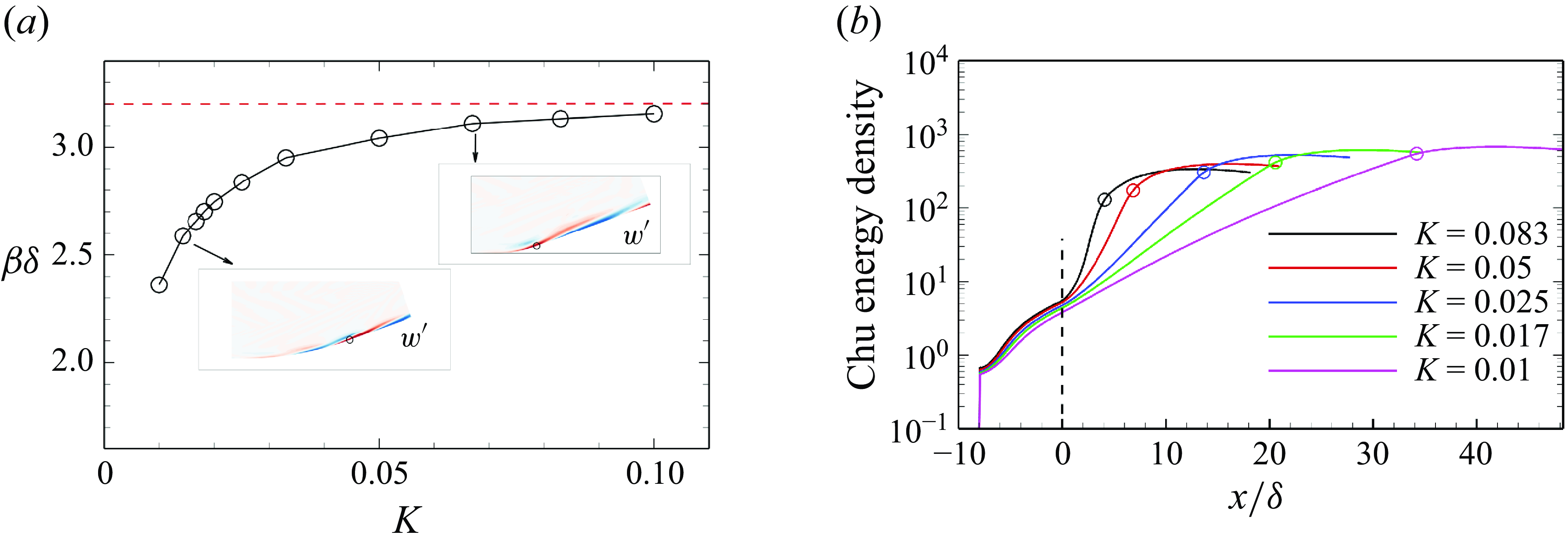
Figure 18. ( $ a$
) Optimal wavenumbers and (
$ a$
) Optimal wavenumbers and ( $ b$
) corresponding distributions of integrated Chu energy density at different concave curvatures. The insets in (
$ b$
) corresponding distributions of integrated Chu energy density at different concave curvatures. The insets in ( $ a$
) represent the real parts of
$ a$
) represent the real parts of $ w^{\prime}$
of the optimal responses, in the cases
$ w^{\prime}$
of the optimal responses, in the cases $ K=0.014$
and
$ K=0.014$
and $ K=0.067$
, and the red dashed line indicates
$ K=0.067$
, and the red dashed line indicates $ \beta \delta =3.2$
. The black dashed line in (
$ \beta \delta =3.2$
. The black dashed line in ( $ b$
) marks the beginning of the concave surface, while the open circles in (
$ b$
) marks the beginning of the concave surface, while the open circles in ( $ b$
) represent the ends of the concave surfaces.
$ b$
) represent the ends of the concave surfaces.
The second geometric parameter is the curvature radius $ r$
, which corresponds to the concave curvature
$ r$
, which corresponds to the concave curvature $ K$
. Figure 18(
$ K$
. Figure 18( $ a$
) illustrates the optimal wavenumbers at different concave curvatures for a constant total turning angle
$ a$
) illustrates the optimal wavenumbers at different concave curvatures for a constant total turning angle $ \varphi =20^{\circ }$
. The optimal wavenumber rises sharply at small
$ \varphi =20^{\circ }$
. The optimal wavenumber rises sharply at small $ K$
and more gradually at larger values, with only a minor increase between
$ K$
and more gradually at larger values, with only a minor increase between $ K=0.083$
and
$ K=0.083$
and $ K=0.1$
. It is predicted that further increasing
$ K=0.1$
. It is predicted that further increasing $ K$
will cause the optimal wavenumber to converge towards a specific constant value, approximately
$ K$
will cause the optimal wavenumber to converge towards a specific constant value, approximately $ \beta \delta =3.2$
, as indicated by the red dashed line in the figure. The coherent structures in the cases
$ \beta \delta =3.2$
, as indicated by the red dashed line in the figure. The coherent structures in the cases $ K=0.014$
and
$ K=0.014$
and $ K=0.067$
shown in the insets of figure 18(
$ K=0.067$
shown in the insets of figure 18( $ a$
) resemble those at
$ a$
) resemble those at $ K =0.02$
in figure 5, which implies that changes in concave curvature do not affect the coherent structures qualitatively.
$ K =0.02$
in figure 5, which implies that changes in concave curvature do not affect the coherent structures qualitatively.
Figure 18( $ b$
) presents the integrated Chu energy density along the wall-normal direction at different concave curvatures at their respective optimal wavenumbers. The exponentially increasing trends in the concave region are evident for cases at different curvatures. Unlike the consistent trend observed in figure 17(
$ b$
) presents the integrated Chu energy density along the wall-normal direction at different concave curvatures at their respective optimal wavenumbers. The exponentially increasing trends in the concave region are evident for cases at different curvatures. Unlike the consistent trend observed in figure 17( $ b$
), the trends differ for various curvatures. Specifically, a large curvature results in a rapid increase in Chu energy density. The rapid increase of fluctuation energy in a large concave curvature region aligns with previous experimental findings (Jayaram et al. Reference Jayaram, Taylor and Smits1987). Although the region influenced by the centrifugal effects is short at a large curvature, the Chu energy density still reaches a high level.
$ b$
), the trends differ for various curvatures. Specifically, a large curvature results in a rapid increase in Chu energy density. The rapid increase of fluctuation energy in a large concave curvature region aligns with previous experimental findings (Jayaram et al. Reference Jayaram, Taylor and Smits1987). Although the region influenced by the centrifugal effects is short at a large curvature, the Chu energy density still reaches a high level.
An infinite curvature $ K\rightarrow \infty$
represents a
$ K\rightarrow \infty$
represents a $ 20^{\circ }$
compression ramp configuration. However, achieving
$ 20^{\circ }$
compression ramp configuration. However, achieving $ K\rightarrow \infty$
for a streamline in real flows is impossible because an adverse pressure gradient will cause a separation bubble that alters the curvature. Figure 19(
$ K\rightarrow \infty$
for a streamline in real flows is impossible because an adverse pressure gradient will cause a separation bubble that alters the curvature. Figure 19( $ a$
) shows the concave curvature distributions of three streamlines passing through
$ a$
) shows the concave curvature distributions of three streamlines passing through $(x_0,0.01\delta)$
,
$(x_0,0.01\delta)$
, $(x_0,0.05\delta)$
and
$(x_0,0.05\delta)$
and $(x_0,0.15\delta)$
in a
$(x_0,0.15\delta)$
in a $ 20^{\circ }$
compression ramp case. The concave curvatures are at large values near the separation and reattachment points, but remain small close to the corner. The two pronounced curvature peaks near these points are significantly larger than the critical value 0.01 (Hoffmann et al. Reference Hoffmann, Muck and Bradshaw1985), making the optimal wavenumber approach the upper boundary
$ 20^{\circ }$
compression ramp case. The concave curvatures are at large values near the separation and reattachment points, but remain small close to the corner. The two pronounced curvature peaks near these points are significantly larger than the critical value 0.01 (Hoffmann et al. Reference Hoffmann, Muck and Bradshaw1985), making the optimal wavenumber approach the upper boundary $ \beta \delta =3.2$
under the individual influence of the centrifugal effects. However, in a dynamic system of turbulent flows with a separation bubble, bubble dynamics and the centrifugal effects coexist. The bubble dynamics may dominate the centrifugal effects on the main amplification mechanism in the dynamic system predicted by resolvent analysis. As mentioned by Hao (Reference Hao2023), in a
$ \beta \delta =3.2$
under the individual influence of the centrifugal effects. However, in a dynamic system of turbulent flows with a separation bubble, bubble dynamics and the centrifugal effects coexist. The bubble dynamics may dominate the centrifugal effects on the main amplification mechanism in the dynamic system predicted by resolvent analysis. As mentioned by Hao (Reference Hao2023), in a $ 25^{\circ }$
compression ramp case, the local maxima of the optimal gain are related to the bubble dynamics, while the Görtler instability is insignificant.
$ 25^{\circ }$
compression ramp case, the local maxima of the optimal gain are related to the bubble dynamics, while the Görtler instability is insignificant.
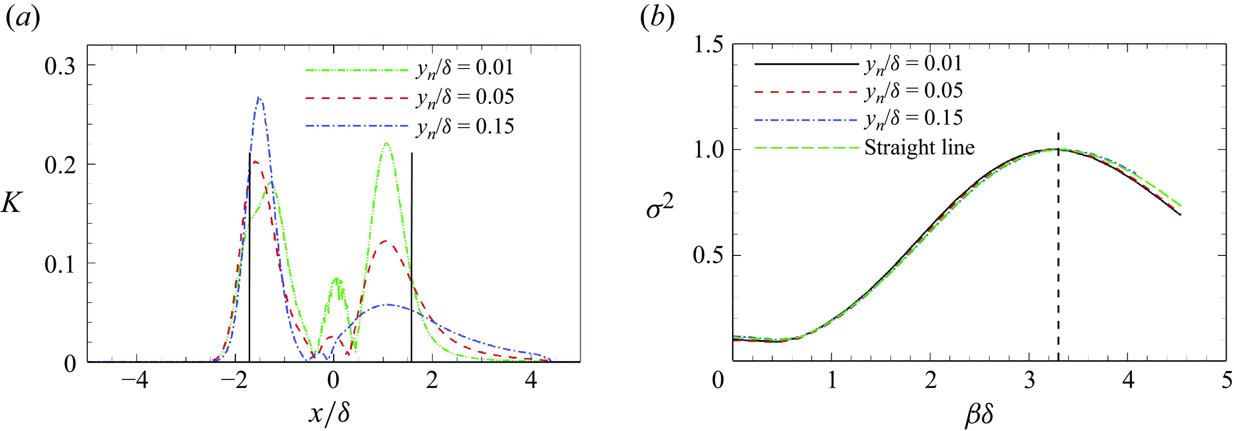
Figure 19. ( $ a$
) Distributions of concave curvatures of three streamlines passing through
$ a$
) Distributions of concave curvatures of three streamlines passing through $(x_0,0.01\delta)$
,
$(x_0,0.01\delta)$
, $(x_0,0.05\delta)$
and
$(x_0,0.05\delta)$
and $(x_0,0.15\delta)$
in a
$(x_0,0.15\delta)$
in a $ 20^{\circ }$
compression ramp case. (
$ 20^{\circ }$
compression ramp case. ( $ b$
) Normalised optimal gains as functions of spanwise wavenumbers
$ b$
) Normalised optimal gains as functions of spanwise wavenumbers $ \beta \delta$
at
$ \beta \delta$
at $ St=0.036$
for different geometries. The black lines in (
$ St=0.036$
for different geometries. The black lines in ( $ a$
) denote the mean separation and reattachment points. Local maxima at
$ a$
) denote the mean separation and reattachment points. Local maxima at $ \beta \delta =3.3$
are indicated by the black dashed line in (
$ \beta \delta =3.3$
are indicated by the black dashed line in ( $ b$
).
$ b$
).
To validate the predicted upper boundary value and illustrate the large concave curvature effects, the three streamlines in figure 19( $ a$
) are established as walls of new geometries to isolate the separation bubble. For comparison, an additional geometry with a straight line connecting the separation and reattachment points is also considered. Figure 19(
$ a$
) are established as walls of new geometries to isolate the separation bubble. For comparison, an additional geometry with a straight line connecting the separation and reattachment points is also considered. Figure 19( $ b$
) compares the optimal gains obtained using the four new geometries. As expected, all four cases share an analogous trend and a common peak
$ b$
) compares the optimal gains obtained using the four new geometries. As expected, all four cases share an analogous trend and a common peak $ \beta \delta =3.3$
, i.e.
$ \beta \delta =3.3$
, i.e. $ \lambda _{z}=1.9\delta$
, which is close to the
$ \lambda _{z}=1.9\delta$
, which is close to the $ 2\delta$
Görtler structures reported by experiments (Schuelein & Trofimov Reference Schuelein and Trofimov2011; Zhuang et al. Reference Zhuang, Tan, Liu, Zhang and Ling2017) and numerical simulations (Loginov, Adams & Zheltovodov Reference Loginov, Adams and Zheltovodov2006; Priebe et al. Reference Priebe, Tu, Rowley and Martín2016) in compression ramp cases. Furthermore, the Görtler structures are also found in impinging shock interactions (Pasquariello, Hickel & Adams Reference Pasquariello, Hickel and Adams2017; Li et al. Reference Li, Zhang, Yu, Lin, Tan and Sun2022) where separation bubbles also exist. Obviously, the coupled effects of separation bubbles with the Görtler instability influence the Görtler structures slightly. Therefore, the upper boundary value provides some valuable insights into characterising the spanwise scales of Görtler vortices with separation bubbles.
$ 2\delta$
Görtler structures reported by experiments (Schuelein & Trofimov Reference Schuelein and Trofimov2011; Zhuang et al. Reference Zhuang, Tan, Liu, Zhang and Ling2017) and numerical simulations (Loginov, Adams & Zheltovodov Reference Loginov, Adams and Zheltovodov2006; Priebe et al. Reference Priebe, Tu, Rowley and Martín2016) in compression ramp cases. Furthermore, the Görtler structures are also found in impinging shock interactions (Pasquariello, Hickel & Adams Reference Pasquariello, Hickel and Adams2017; Li et al. Reference Li, Zhang, Yu, Lin, Tan and Sun2022) where separation bubbles also exist. Obviously, the coupled effects of separation bubbles with the Görtler instability influence the Görtler structures slightly. Therefore, the upper boundary value provides some valuable insights into characterising the spanwise scales of Görtler vortices with separation bubbles.
One might argue that the shock structures of the four cases are significantly different from those with the separation bubble in the $ 20^{\circ }$
compression ramp case. However, an equal strength of the concave curvature is the essential parameter for separately investigating the Görtler vortices in compression ramp cases.
$ 20^{\circ }$
compression ramp case. However, an equal strength of the concave curvature is the essential parameter for separately investigating the Görtler vortices in compression ramp cases.
5.3. Freestream parameters
Additional cases are considered to investigate the influence of freestream parameters on the spanwise scales of Görtler vortices, including the unit Reynolds number $ {Re}_{\infty }$
, Mach number
$ {Re}_{\infty }$
, Mach number $ {M}_{\infty }$
, and temperature ratio
$ {M}_{\infty }$
, and temperature ratio $ {T}_{w}/{T}_{\infty }$
. We isolate the influence of one parameter by keeping the other two parameters unchanged. The cases with the original freestream parameters are referred to as the baseline cases.
$ {T}_{w}/{T}_{\infty }$
. We isolate the influence of one parameter by keeping the other two parameters unchanged. The cases with the original freestream parameters are referred to as the baseline cases.

Figure 20. Normalised optimal gains as functions of spanwise wavenumbers $ \beta \delta$
at different (
$ \beta \delta$
at different ( $ a$
) Mach number, (
$ a$
) Mach number, ( $ b$
) temperature ratio, and (
$ b$
) temperature ratio, and ( $ c$
) Reynolds number, at
$ c$
) Reynolds number, at $ r=50\delta$
and
$ r=50\delta$
and $ \varphi =20^{\circ }$
. The red arrows in (a,b) indicate increasing trends, and the black dashed line in (
$ \varphi =20^{\circ }$
. The red arrows in (a,b) indicate increasing trends, and the black dashed line in ( $ c$
) means a local maximum.
$ c$
) means a local maximum.
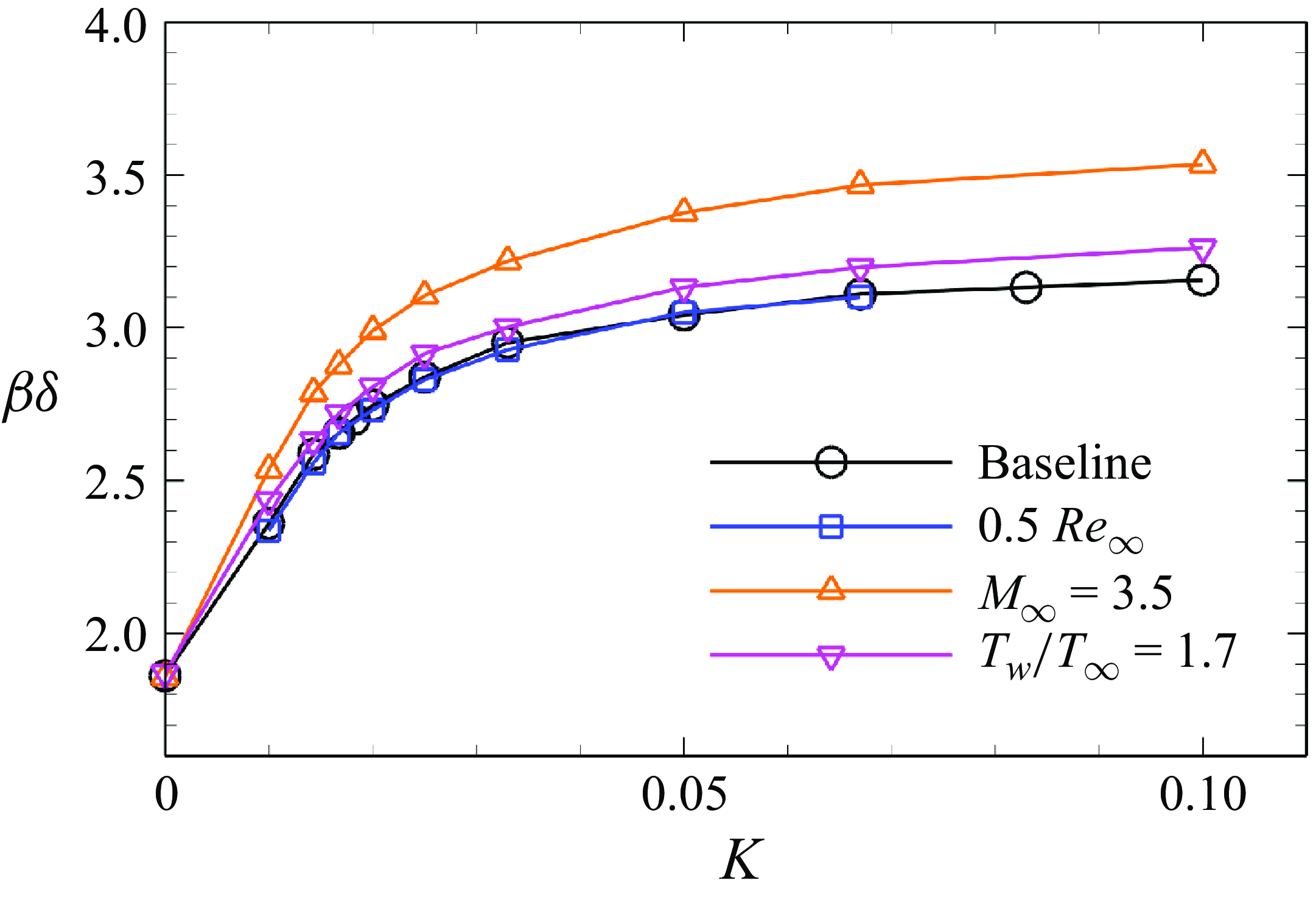
Figure 21. Preferential wavenumbers as a function of concave curvature for a constant turning angle $ \varphi =20^{\circ }$
.
$ \varphi =20^{\circ }$
.
Optimal gains as a function of the scaled wavenumber $ \beta \delta$
at different freestream parameters are shown in figure 20. The optimal wavenumber increases with an increase in
$ \beta \delta$
at different freestream parameters are shown in figure 20. The optimal wavenumber increases with an increase in $ {M}_{\infty }$
. A similar increasing trend is shown in figure 20(
$ {M}_{\infty }$
. A similar increasing trend is shown in figure 20( $ b$
) when decreasing the temperature ratio
$ b$
) when decreasing the temperature ratio $ {T}_{w}/{T}_{\infty }$
, although the change is slight. Figure 20(
$ {T}_{w}/{T}_{\infty }$
, although the change is slight. Figure 20( $ c$
) depicts the optimal gains at different freestream Reynolds numbers
$ c$
) depicts the optimal gains at different freestream Reynolds numbers $ Re_{\infty }$
. The optimal wavenumber
$ Re_{\infty }$
. The optimal wavenumber $ \beta \delta =2.73$
is shared by different Reynolds number cases, implying that the optimal wavenumber predicted by resolvent analysis is independent of the freestream Reynolds number, when normalised using the boundary-layer thickness.
$ \beta \delta =2.73$
is shared by different Reynolds number cases, implying that the optimal wavenumber predicted by resolvent analysis is independent of the freestream Reynolds number, when normalised using the boundary-layer thickness.
Figure 21 shows the optimal wavenumbers as a function of concave curvature under different flow conditions. Trends similar to the baseline cases are observed at different flow parameters, with a rapid rise when $ K$
is small, and a slow rise when
$ K$
is small, and a slow rise when $ K$
is large. The upper boundary corresponding to
$ K$
is large. The upper boundary corresponding to $ K\rightarrow \infty$
can also be determined for various freestream parameters. As discussed in § 5.2, the upper boundary value can be regarded as an approximate wavenumber of the Görtler vortices in cases with a separation bubble. Hence the Mach number effect can be verified qualitatively by different supersonic or hypersonic compression ramp cases. At
$ K\rightarrow \infty$
can also be determined for various freestream parameters. As discussed in § 5.2, the upper boundary value can be regarded as an approximate wavenumber of the Görtler vortices in cases with a separation bubble. Hence the Mach number effect can be verified qualitatively by different supersonic or hypersonic compression ramp cases. At $ {M}_{\infty } =2.95$
, the structures of
$ {M}_{\infty } =2.95$
, the structures of $ 2\delta$
were observed from time-averaged skin friction distribution by Loginov et al. (Reference Loginov, Adams and Zheltovodov2006). When
$ 2\delta$
were observed from time-averaged skin friction distribution by Loginov et al. (Reference Loginov, Adams and Zheltovodov2006). When $ {M}_{\infty } =6$
, the Görtler structures downstream of the separation bubble are changed to
$ {M}_{\infty } =6$
, the Görtler structures downstream of the separation bubble are changed to $ 1.2\delta$
, as shown by Guo et al. (Reference Guo, Zhang, Zhu and Li2024). The decrease in the wavelength of Görtler vortices is consistent with our findings. The decreasing trend may be related to compressibility effects, which will be investigated in a future study. Furthermore, the Reynolds number independent relation is verified, as the optimal wavenumbers overlap for the two Reynolds number cases at different curvatures, in agreement with experimental findings by Schuelein & Trofimov (Reference Schuelein and Trofimov2011) in turbulent separated flows.
$ 1.2\delta$
, as shown by Guo et al. (Reference Guo, Zhang, Zhu and Li2024). The decrease in the wavelength of Görtler vortices is consistent with our findings. The decreasing trend may be related to compressibility effects, which will be investigated in a future study. Furthermore, the Reynolds number independent relation is verified, as the optimal wavenumbers overlap for the two Reynolds number cases at different curvatures, in agreement with experimental findings by Schuelein & Trofimov (Reference Schuelein and Trofimov2011) in turbulent separated flows.
Our results offer quantitative insights into predicting the scale of Görtler vortices. Future efforts should focus on exploring the coupling effects between separation bubbles and Görtler instability in compression ramps, as well as impinging shock interactions in turbulent flows.
6. Occurrence of Görtler instability
The results from resolvent analysis and LSA are examined in § 4.1. The LSA provides accurate predictions for both the spatial growth rate and the spanwise wavelength of the Görtler mode, consistent with values predicted by resolvent analysis. Consequently, LSA can be employed to estimate the spatial growth rate of the Görtler mode, thereby assessing the occurrence of Görtler vortices.
Two parameters are usually used to evaluate Görtler instability in turbulent flows: the concave curvature $ K$
, and the Görtler number
$ K$
, and the Görtler number $ {G}_{T}$
. The definition of
$ {G}_{T}$
. The definition of $ {G}_{T}$
in laminar flows is given by
$ {G}_{T}$
in laminar flows is given by
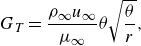 \begin{equation} {G}_{T}=\frac {{\rho }_{\infty } {u}_{\infty }}{{\mu }_{\infty } }\theta \sqrt {\frac {\theta }{r}}, \end{equation}
where $ \theta$
represents the boundary-layer momentum thickness. Tani (Reference Tani1962) suggested using the eddy viscosity
$ \theta$
represents the boundary-layer momentum thickness. Tani (Reference Tani1962) suggested using the eddy viscosity $ \mu _{t}$
to replace the molecular viscosity
$ \mu _{t}$
to replace the molecular viscosity $ {\mu }_{\infty }$
for defining
$ {\mu }_{\infty }$
for defining $ {G}_{T}$
in turbulent flows. He followed a simple assumption of a constant eddy viscosity
$ {G}_{T}$
in turbulent flows. He followed a simple assumption of a constant eddy viscosity $ \mu _{t}=0.018 {\rho }_{\infty } {u}_{\infty }\delta ^{*}$
for outer layers of incompressible TBLs (Clauser Reference Clauser1956), where
$ \mu _{t}=0.018 {\rho }_{\infty } {u}_{\infty }\delta ^{*}$
for outer layers of incompressible TBLs (Clauser Reference Clauser1956), where $ {\delta }^{*}$
is the boundary-layer displacement thickness. This leads to the following expression for the turbulent Görtler number:
$ {\delta }^{*}$
is the boundary-layer displacement thickness. This leads to the following expression for the turbulent Görtler number:
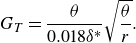 \begin{equation} {G}_{T}=\frac {\theta }{0.018\delta ^{*} } \sqrt {\frac {\theta }{r}} . \end{equation}
Smits & Dussauge (Reference Smits and Dussauge2006) extended the turbulent $ {G}_{T}$
to compressible flows while using the same assumption of a constant eddy viscosity. However, the assumption of a constant
$ {G}_{T}$
to compressible flows while using the same assumption of a constant eddy viscosity. However, the assumption of a constant $ \mu _{t}$
in outer layers of TBLs may not be appropriate. One can refer to Abe & Antonia (Reference Abe and Antonia2019) and figure 16(
$ \mu _{t}$
in outer layers of TBLs may not be appropriate. One can refer to Abe & Antonia (Reference Abe and Antonia2019) and figure 16( $ a$
) for distributions of
$ a$
) for distributions of $ \mu _{t}$
in incompressible and compressible flows, respectively. Furthermore, the empirical formula overestimates
$ \mu _{t}$
in incompressible and compressible flows, respectively. Furthermore, the empirical formula overestimates $ \mu _{t}$
in the outer layer of TBLs. For instance, the formula gives
$ \mu _{t}$
in the outer layer of TBLs. For instance, the formula gives $ {\mu }_{t}/{\mu }_{\infty }=365$
, which is significantly higher than the peak values
$ {\mu }_{t}/{\mu }_{\infty }=365$
, which is significantly higher than the peak values $ {\mu }_{t}/{\mu }_{\infty }=125$
and 86 at the reference station
$ {\mu }_{t}/{\mu }_{\infty }=125$
and 86 at the reference station $ x_{0}$
from RANS and LES. Such an overestimation causes an underestimation of the turbulent
$ x_{0}$
from RANS and LES. Such an overestimation causes an underestimation of the turbulent $ {G}_{T}$
. Different modelling approaches for
$ {G}_{T}$
. Different modelling approaches for $ \mu _{t}$
based on DNS/LES databases and RANS models of zero pressure gradient flat plates lead to slight variations in the peak
$ \mu _{t}$
based on DNS/LES databases and RANS models of zero pressure gradient flat plates lead to slight variations in the peak $ \mu _{t, peak}$
values in TBLs. To investigate the critical
$ \mu _{t, peak}$
values in TBLs. To investigate the critical $ G_{T}$
under different flow conditions, we choose the peak value
$ G_{T}$
under different flow conditions, we choose the peak value $ \mu _{t, peak}$
at the reference station
$ \mu _{t, peak}$
at the reference station $ x_{0}$
from the RANS results (see figure 16
$ x_{0}$
from the RANS results (see figure 16 $ a$
) as the reference value to replace the
$ a$
) as the reference value to replace the $ {\mu }_{\infty }$
in calculating the turbulent
$ {\mu }_{\infty }$
in calculating the turbulent $ {G}_{T}$
, given as
$ {G}_{T}$
, given as
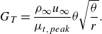 \begin{equation} {G}_{T}=\frac {{\rho }_{\infty } {u}_{\infty }}{{\mu }_{t, peak } }\theta \sqrt {\frac {\theta }{r}}. \end{equation}
As we mentioned before, the critical value $ K=0.01$
for inducing streamwise vortices was proposed by Hoffmann et al. (Reference Hoffmann, Muck and Bradshaw1985), and used by Loginov et al. (Reference Loginov, Adams and Zheltovodov2006) and Priebe et al. (Reference Priebe, Tu, Rowley and Martín2016) in turbulent separated flows. Smits & Dussauge (Reference Smits and Dussauge2006) also suggested that the critical value
$ K=0.01$
for inducing streamwise vortices was proposed by Hoffmann et al. (Reference Hoffmann, Muck and Bradshaw1985), and used by Loginov et al. (Reference Loginov, Adams and Zheltovodov2006) and Priebe et al. (Reference Priebe, Tu, Rowley and Martín2016) in turbulent separated flows. Smits & Dussauge (Reference Smits and Dussauge2006) also suggested that the critical value $ K$
is approximately 0.03 in Mach 3 flows, and changes as Mach number changes. However, our LES results clearly show that Görtler vortices begin to manifest at
$ K$
is approximately 0.03 in Mach 3 flows, and changes as Mach number changes. However, our LES results clearly show that Görtler vortices begin to manifest at $ K=0.02$
, indicating that the value 0.03 may be somewhat overestimated.
$ K=0.02$
, indicating that the value 0.03 may be somewhat overestimated.
Moreover, the critical $ {G}_{T}$
for turbulent flows has not been established (Floryan Reference Floryan1991). Many researchers (Loginov et al. Reference Loginov, Adams and Zheltovodov2006; Priebe et al. Reference Priebe, Tu, Rowley and Martín2016; Tong et al. Reference Tong, Li, Duan and Yu2017) have used the critical value 0.6 in laminar flows (Görtler Reference Görtler1954) as a criterion for turbulent flows (calculated from (6.2)). However, the value would increase to a range 1.8–2.4 if calculated using the correct
$ {G}_{T}$
for turbulent flows has not been established (Floryan Reference Floryan1991). Many researchers (Loginov et al. Reference Loginov, Adams and Zheltovodov2006; Priebe et al. Reference Priebe, Tu, Rowley and Martín2016; Tong et al. Reference Tong, Li, Duan and Yu2017) have used the critical value 0.6 in laminar flows (Görtler Reference Görtler1954) as a criterion for turbulent flows (calculated from (6.2)). However, the value would increase to a range 1.8–2.4 if calculated using the correct $ {\mu }_{t}$
. Given that the growth rate predicted by LSA agrees well with the resolvent analysis result, LSA is used in this study to determine the critical
$ {\mu }_{t}$
. Given that the growth rate predicted by LSA agrees well with the resolvent analysis result, LSA is used in this study to determine the critical $ {G}_{T}$
based on (6.3).
$ {G}_{T}$
based on (6.3).
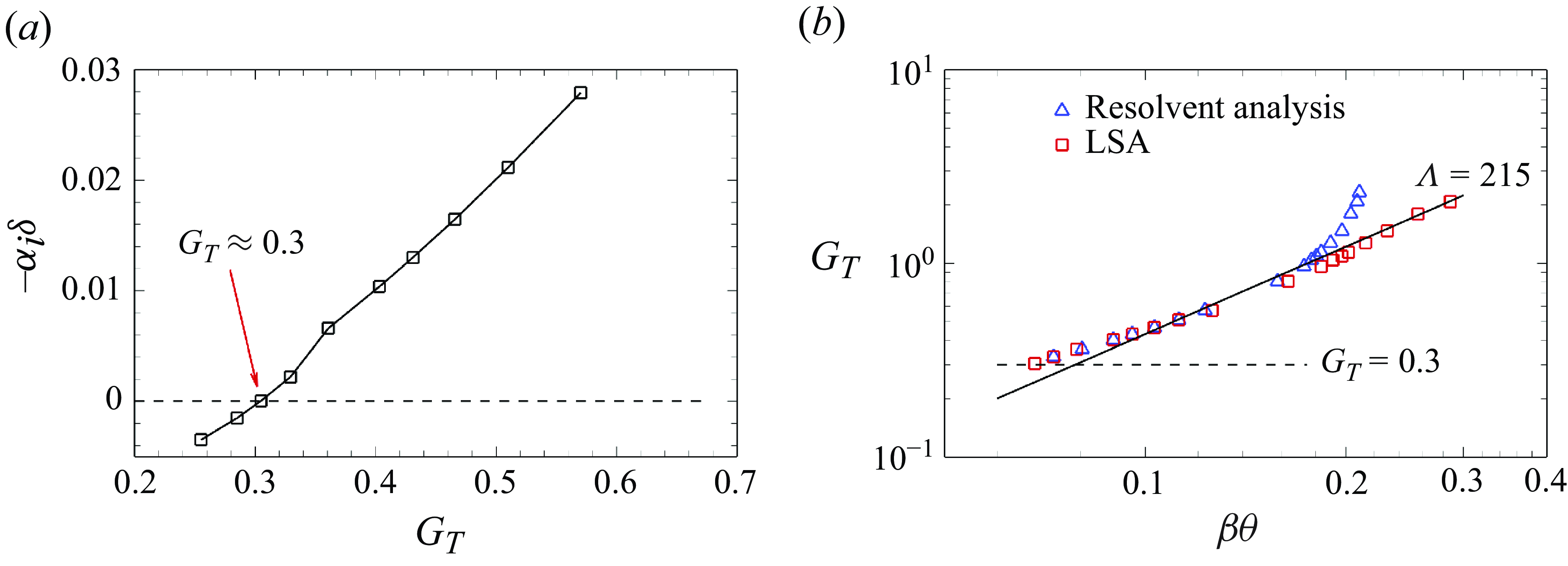
Figure 22. ( $ a$
) The maximum spatial growth rate
$ a$
) The maximum spatial growth rate $ -\alpha _{i} \delta$
at station
$ -\alpha _{i} \delta$
at station $ \varphi = 10^{\circ }$
predicted by LSA at
$ \varphi = 10^{\circ }$
predicted by LSA at $ St=0.036$
. (
$ St=0.036$
. ( $ b$
) The optimal wavenumber
$ b$
) The optimal wavenumber $ \beta \theta$
from resolvent analysis, along with the most unstable wavenumber
$ \beta \theta$
from resolvent analysis, along with the most unstable wavenumber $ \beta \theta$
from LSA of the baseline cases as a function of Görtler number
$ \beta \theta$
from LSA of the baseline cases as a function of Görtler number $ G_{T}$
. The Görtler numbers are extracted from streamlines passing through
$ G_{T}$
. The Görtler numbers are extracted from streamlines passing through $(x_0,0.5\delta)$
. The black dashed line in (
$(x_0,0.5\delta)$
. The black dashed line in ( $ a$
) indicates zero growth rate. The black line in (
$ a$
) indicates zero growth rate. The black line in ( $ b$
) indicates
$ b$
) indicates $ \Lambda =215$
, where
$ \Lambda =215$
, where $ \Lambda =( {{\rho }_{\infty } {u}_{\infty }}/{{\mu }_{t, peak } }){\lambda }_{z}\sqrt {{{\lambda }_{z}}/{r}}$
is a dimensionless wavelength parameter (Saric et al. Reference Saric1994).
$ \Lambda =( {{\rho }_{\infty } {u}_{\infty }}/{{\mu }_{t, peak } }){\lambda }_{z}\sqrt {{{\lambda }_{z}}/{r}}$
is a dimensionless wavelength parameter (Saric et al. Reference Saric1994).
Figure 22( $ a$
) presents the maximum spatial growth rates at station
$ a$
) presents the maximum spatial growth rates at station $ \varphi = 10^{\circ }$
predicted by LSA, with the peak
$ \varphi = 10^{\circ }$
predicted by LSA, with the peak $ {G}_{T}$
of streamlines passing through
$ {G}_{T}$
of streamlines passing through $(x_0,0.5\delta)$
for the baseline cases across varying concave curvatures. It can be observed that as
$(x_0,0.5\delta)$
for the baseline cases across varying concave curvatures. It can be observed that as $ {G}_{T}$
progressively diminishes, the maximum growth rate
$ {G}_{T}$
progressively diminishes, the maximum growth rate $ -\alpha _{i} \delta$
exhibits a concomitant decline. A maximum spatial growth rate
$ -\alpha _{i} \delta$
exhibits a concomitant decline. A maximum spatial growth rate $ -\alpha _{i} \delta \lt 0$
signifies that the Görtler mode remains unexcited, resulting in the absence of Görtler vortices. A zero growth rate is attained at
$ -\alpha _{i} \delta \lt 0$
signifies that the Görtler mode remains unexcited, resulting in the absence of Görtler vortices. A zero growth rate is attained at $ {G}_{T}= 0.3$
, corresponding to
$ {G}_{T}= 0.3$
, corresponding to $ K= 0.00143$
. The predicted
$ K= 0.00143$
. The predicted $ {G}_{T}=0.3$
is close to the laminar critical value 0.6 (Görtler Reference Görtler1954), but the curvature
$ {G}_{T}=0.3$
is close to the laminar critical value 0.6 (Görtler Reference Görtler1954), but the curvature $ K=0.00143$
is significantly lower than the experimentally obtained empirical value 0.01 for turbulent flows (Hoffmann et al. Reference Hoffmann, Muck and Bradshaw1985). The critical
$ K=0.00143$
is significantly lower than the experimentally obtained empirical value 0.01 for turbulent flows (Hoffmann et al. Reference Hoffmann, Muck and Bradshaw1985). The critical $ G_{T}$
becomes 0.45 when using
$ G_{T}$
becomes 0.45 when using $ \mu _{t, peak}$
from LES. Both values are much lower than the previous empirical range 1.8–2.4 (calculated using (6.3)). It should be noted that different modelling methods for
$ \mu _{t, peak}$
from LES. Both values are much lower than the previous empirical range 1.8–2.4 (calculated using (6.3)). It should be noted that different modelling methods for $ \mu _{t}$
may lead to a slight change in the critical
$ \mu _{t}$
may lead to a slight change in the critical $ G_{T}$
values, although the trends remain similar. Essentially, the critical value 0.6 in laminar flows (or 0.4638 in Floryan & Saric Reference Floryan and Saric1982) is an empirical guideline at the incompressible limit. However, El-Hady & Verma (Reference El-Hady and Verma1984) found that the critical
$ G_{T}$
values, although the trends remain similar. Essentially, the critical value 0.6 in laminar flows (or 0.4638 in Floryan & Saric Reference Floryan and Saric1982) is an empirical guideline at the incompressible limit. However, El-Hady & Verma (Reference El-Hady and Verma1984) found that the critical $ G_{T}$
increases with rising
$ G_{T}$
increases with rising $ M_{\infty }$
, which indicates that this guideline may not be suitable for all laminar flow scenarios, such as varying Mach numbers and wall temperatures. There may not be a solid criterion for compressible laminar and turbulent flows. Thus we do not aim to specify a precise critical
$ M_{\infty }$
, which indicates that this guideline may not be suitable for all laminar flow scenarios, such as varying Mach numbers and wall temperatures. There may not be a solid criterion for compressible laminar and turbulent flows. Thus we do not aim to specify a precise critical $ G_{T}$
, but rather provide an approximate range 0.3–0.45 to offer meaningful guidance on the occurrence of Görtler vortices in compressible turbulent flows. Future work will incorporate multi-fidelity
$ G_{T}$
, but rather provide an approximate range 0.3–0.45 to offer meaningful guidance on the occurrence of Görtler vortices in compressible turbulent flows. Future work will incorporate multi-fidelity $ {\mu }_{t}$
from DNS/LES datasets to refine this range, but our current results provide a conservative estimate for design purposes.
$ {\mu }_{t}$
from DNS/LES datasets to refine this range, but our current results provide a conservative estimate for design purposes.
It is worth noting that the critical values obtained, whether for laminar or turbulent flows, are only of reference significance. Only when $ G_{T}$
is much larger than the critical value will the Görtler vortices manifest obviously in flows. In practice, determining the critical
$ G_{T}$
is much larger than the critical value will the Görtler vortices manifest obviously in flows. In practice, determining the critical $ G_{T}$
experimentally poses significant challenges due to the low energy growth rates, which necessitates a long concave surface to allow Görtler vortices to develop observable amplitudes. However, the finite length of models artificially truncates this growth process, leading to overestimated critical
$ G_{T}$
experimentally poses significant challenges due to the low energy growth rates, which necessitates a long concave surface to allow Görtler vortices to develop observable amplitudes. However, the finite length of models artificially truncates this growth process, leading to overestimated critical $ G_{T}$
values – often exceeding theoretical predictions by orders of magnitude. Consequently, Görtler vortices may remain undetected even in configurations where
$ G_{T}$
values – often exceeding theoretical predictions by orders of magnitude. Consequently, Görtler vortices may remain undetected even in configurations where $ G_{T}$
far surpasses the theoretical threshold. The determined
$ G_{T}$
far surpasses the theoretical threshold. The determined $ G_{T}$
and
$ G_{T}$
and $ K$
by LSA represent theoretical lower bounds.
$ K$
by LSA represent theoretical lower bounds.
Figure 22( $b$
) compares the optimal wavenumber from resolvent analysis with the most unstable wavenumber obtained from LSA as a function of
$b$
) compares the optimal wavenumber from resolvent analysis with the most unstable wavenumber obtained from LSA as a function of $ {G}_{T}$
for the baseline cases. When
$ {G}_{T}$
for the baseline cases. When $ {G}_{T}$
is small, i.e. the concave curvature is small, the wavenumbers from both methods align closely with each other. Notably, both analyses yield wavenumbers that fall along the line
$ {G}_{T}$
is small, i.e. the concave curvature is small, the wavenumbers from both methods align closely with each other. Notably, both analyses yield wavenumbers that fall along the line $ \Lambda =215$
when
$ \Lambda =215$
when $ \beta \theta \lt 0.18$
, which is consistent with the constant-
$ \beta \theta \lt 0.18$
, which is consistent with the constant- $ \Lambda$
assumption in laminar flows (Tani Reference Tani1962; Saric et al. Reference Saric1994). However, a discrepancy occurs when
$ \Lambda$
assumption in laminar flows (Tani Reference Tani1962; Saric et al. Reference Saric1994). However, a discrepancy occurs when $ {G}_{T}\gt 1.2$
. In this case, the most unstable wavenumber from LSA remains on the line
$ {G}_{T}\gt 1.2$
. In this case, the most unstable wavenumber from LSA remains on the line $ \Lambda =215$
, while the optimal wavenumber from resolvent analysis gradually converges to a constant value as
$ \Lambda =215$
, while the optimal wavenumber from resolvent analysis gradually converges to a constant value as $ {G}_{T}$
increases, in agreement with the upper boundary value in figure 18. This discrepancy is attributed to non-parallelism and non-modal effects (Hanifi et al. Reference Hanifi, Schmid and Henningson1996; Tumin & Reshotko Reference Tumin and Reshotko2003). Additionally, figure 22(
$ {G}_{T}$
increases, in agreement with the upper boundary value in figure 18. This discrepancy is attributed to non-parallelism and non-modal effects (Hanifi et al. Reference Hanifi, Schmid and Henningson1996; Tumin & Reshotko Reference Tumin and Reshotko2003). Additionally, figure 22( $b$
) also provides an approximation for the spanwise wavenumbers of Görtler vortices within the Görtler number range 0.3–1.2.
$b$
) also provides an approximation for the spanwise wavenumbers of Görtler vortices within the Görtler number range 0.3–1.2.
7. Conclusions
The spatial–temporal features of Görtler vortices in supersonic turbulent flows over concave surfaces are investigated using resolvent analysis and LES. Resolvent analysis predicts an optimal response with the spanwise wavelength $ \lambda _{z} \approx 2.4\delta$
and the cut-off frequency
$ \lambda _{z} \approx 2.4\delta$
and the cut-off frequency $St=0.036$
, based on an LES base flow at Mach 2.95 and
$St=0.036$
, based on an LES base flow at Mach 2.95 and $ Re_{\delta }=63\,500$
over a concave surface with a total turning angle
$ Re_{\delta }=63\,500$
over a concave surface with a total turning angle $ \varphi =20^{\circ }$
and curvature radius
$ \varphi =20^{\circ }$
and curvature radius $ r=50 \delta$
. The optimal resolvent mode manifests as streamwise counter-rotating vortices in the concave region, identified as the Görtler vortices, which are consistent with the spatial structures in laminar flows (Görtler Reference Görtler1954; Floryan Reference Floryan1991). The dominant amplification mechanism is the Görtler instability. The integrated Chu energy density increases exponentially in the concave region, with the growth rate closely matching LSA results. Furthermore, the optimal wavelength and mode shapes predicted by LSA also align well with those obtained by resolvent analysis.
$ r=50 \delta$
. The optimal resolvent mode manifests as streamwise counter-rotating vortices in the concave region, identified as the Görtler vortices, which are consistent with the spatial structures in laminar flows (Görtler Reference Görtler1954; Floryan Reference Floryan1991). The dominant amplification mechanism is the Görtler instability. The integrated Chu energy density increases exponentially in the concave region, with the growth rate closely matching LSA results. Furthermore, the optimal wavelength and mode shapes predicted by LSA also align well with those obtained by resolvent analysis.
These predictions are validated against the same LES dataset. The centrifugal effects promote momentum exchange and enhance turbulence intensity, with a second peak of turbulent kinetic energy occurring at $y_{n}/\delta = 0.26$
. The POD analysis is performed on
$y_{n}/\delta = 0.26$
. The POD analysis is performed on $y$
–
$y$
– $z$
slices at stations
$z$
slices at stations $\varphi = 10^{\circ }$
and
$\varphi = 10^{\circ }$
and $20^{\circ }$
. The most energetic spatial structures at the two stations are similar streamwise counter-rotating vortices with spanwise wavelength approximately
$20^{\circ }$
. The most energetic spatial structures at the two stations are similar streamwise counter-rotating vortices with spanwise wavelength approximately $ 2\delta$
. Additionally, coherent structures in the spanwise mid-plane and several
$ 2\delta$
. Additionally, coherent structures in the spanwise mid-plane and several $y$
–
$y$
– $z$
planes are extracted using SPOD. The leading SPOD mode of the spanwise mid-plane peaks at
$z$
planes are extracted using SPOD. The leading SPOD mode of the spanwise mid-plane peaks at $ St = 0.036$
, resembling the optimal output from resolvent analysis at the same frequency. The highest projection coefficient between the leading SPOD mode and the optimal resolvent response is approximately 0.94. The leading SPOD modes at three streamwise stations
$ St = 0.036$
, resembling the optimal output from resolvent analysis at the same frequency. The highest projection coefficient between the leading SPOD mode and the optimal resolvent response is approximately 0.94. The leading SPOD modes at three streamwise stations $\varphi = 10^{\circ }$
,
$\varphi = 10^{\circ }$
, $\varphi = 15^{\circ }$
and
$\varphi = 15^{\circ }$
and $\varphi = 20^{\circ }$
also show similar spanwise structures around
$\varphi = 20^{\circ }$
also show similar spanwise structures around $2\delta$
, consistent with the reconstructed structures using the optimal resolvent mode. The good agreement between the optimal SPOD modes and the resolvent mode implies that resolvent analysis accurately captures the Görtler vortices.
$2\delta$
, consistent with the reconstructed structures using the optimal resolvent mode. The good agreement between the optimal SPOD modes and the resolvent mode implies that resolvent analysis accurately captures the Görtler vortices.
Further investigations are conducted to reveal how the preferential spanwise wavelength of Görtler vortices scales with varying geometric and freestream parameters. The optimal wavelengths are insensitive to the total turning angle beyond a critical value. However, they change as the concave curvature varies at the same turning angle. A limit wavelength $ \lambda _{z}=1.96\delta$
(
$ \lambda _{z}=1.96\delta$
( $\beta \delta =3.2$
), corresponding to infinite curvature
$\beta \delta =3.2$
), corresponding to infinite curvature $ K\rightarrow \infty$
, is identified and validated using a
$ K\rightarrow \infty$
, is identified and validated using a $ 20^{\circ }$
compression ramp case by isolating the separation bubble. This value provides valuable insights into the Görtler instability in turbulent separated flows. The limit wavelength decreases with an increasing Mach number
$ 20^{\circ }$
compression ramp case by isolating the separation bubble. This value provides valuable insights into the Görtler instability in turbulent separated flows. The limit wavelength decreases with an increasing Mach number $ {M}_{\infty }$
and a decreasing temperature ratio
$ {M}_{\infty }$
and a decreasing temperature ratio $ {T}_{w}/{T}_{\infty }$
, remaining unchanged with varying Reynolds number
$ {T}_{w}/{T}_{\infty }$
, remaining unchanged with varying Reynolds number $ Re_{\infty }$
when normalised using the boundary-layer thickness
$ Re_{\infty }$
when normalised using the boundary-layer thickness $ \delta$
. Additionally, a modified definition of the turbulent Görtler number
$ \delta$
. Additionally, a modified definition of the turbulent Görtler number $ G_{T}$
is proposed using the peak eddy viscosity in TBLs. The critical Görtler number
$ G_{T}$
is proposed using the peak eddy viscosity in TBLs. The critical Görtler number $ G_{T}=0.3{-}0.45$
and curvature
$ G_{T}=0.3{-}0.45$
and curvature $ K=0.00143$
are determined by LSA and serve as conservative estimates for evaluating the occurrence of Görtler vortices in the baseline cases.
$ K=0.00143$
are determined by LSA and serve as conservative estimates for evaluating the occurrence of Görtler vortices in the baseline cases.
The optimal forcings responses may provide guidance for flow control strategies. For instance, these optimal forcings can be used through plasma actuators (Ribeiro & Taira Reference Ribeiro and Taira2024) to suppress or enhance the strengths of Görtler vortices. Future studies will discuss control strategies in detail.
Supplementary movies
Supplementary movies are available at https://doi.org/10.1017/jfm.2025.10229.
Funding
This work is supported by the Hong Kong Research Grants Council (nos 15204322 and 25203721) and the National Natural Science Foundation of China (nos 12102377 and 12472239).
Declaration of interests
The authors report no conflict of interest.
Appendix A. Verification of the LES solver
The qualities of the TBL at the reference station $ x_{0}$
are discussed in this appendix. Figure 23(
$ x_{0}$
are discussed in this appendix. Figure 23( $ a$
) compares the mean values of density
$ a$
) compares the mean values of density $ \rho$
, streamwise velocity
$ \rho$
, streamwise velocity $ U$
, and temperature
$ U$
, and temperature $ T$
from LES with the experimental data (Zheltovodov et al. Reference Zheltovodov, Trofimov, Schülein and Yakovlev1990). Good agreement is observed for all three variables. Figure 23(
$ T$
from LES with the experimental data (Zheltovodov et al. Reference Zheltovodov, Trofimov, Schülein and Yakovlev1990). Good agreement is observed for all three variables. Figure 23( $ b$
) presents the Van Driest transformed velocity, defined as
$ b$
) presents the Van Driest transformed velocity, defined as
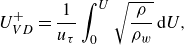 \begin{equation} U_{V D}^{+}=\frac {1}{{u}_{\tau }}\int _{0}^{U}\sqrt {\frac {\rho }{{\rho }_{w}}}\,{\rm d}U , \end{equation}
where $ {u}_{\tau }$
is the wall-fraction velocity, and
$ {u}_{\tau }$
is the wall-fraction velocity, and $ {\rho }_{w}$
is the mean density at the wall. The transformed velocity profile aligns well with the classical solutions, specifically
$ {\rho }_{w}$
is the mean density at the wall. The transformed velocity profile aligns well with the classical solutions, specifically $ U_{V D}^{+}=y^{+}$
and
$ U_{V D}^{+}=y^{+}$
and $ U_{V D}^{+}=(1/0.41)\log (y^{+})+5.1$
, as well as the experimental data (Zheltovodov et al. Reference Zheltovodov, Trofimov, Schülein and Yakovlev1990). Additionally, the density-scaled RMS values are compared with the compressible DNS results (Bernardini & Pirozzoli Reference Bernardini and Pirozzoli2011; Tong et al. Reference Tong, Li, Duan and Yu2017). Our LES results show a good match with these studies.
$ U_{V D}^{+}=(1/0.41)\log (y^{+})+5.1$
, as well as the experimental data (Zheltovodov et al. Reference Zheltovodov, Trofimov, Schülein and Yakovlev1990). Additionally, the density-scaled RMS values are compared with the compressible DNS results (Bernardini & Pirozzoli Reference Bernardini and Pirozzoli2011; Tong et al. Reference Tong, Li, Duan and Yu2017). Our LES results show a good match with these studies.
Figure 24 shows the spanwise correlations at stations $ \varphi =10^{\circ }$
and
$ \varphi =10^{\circ }$
and $ \varphi =20^{\circ }$
. The correlations are negligible when the distance is beyond
$ \varphi =20^{\circ }$
. The correlations are negligible when the distance is beyond $ 1.5\delta$
at both stations, which suggests that the computational domain in this simulation is sufficiently wide.
$ 1.5\delta$
at both stations, which suggests that the computational domain in this simulation is sufficiently wide.
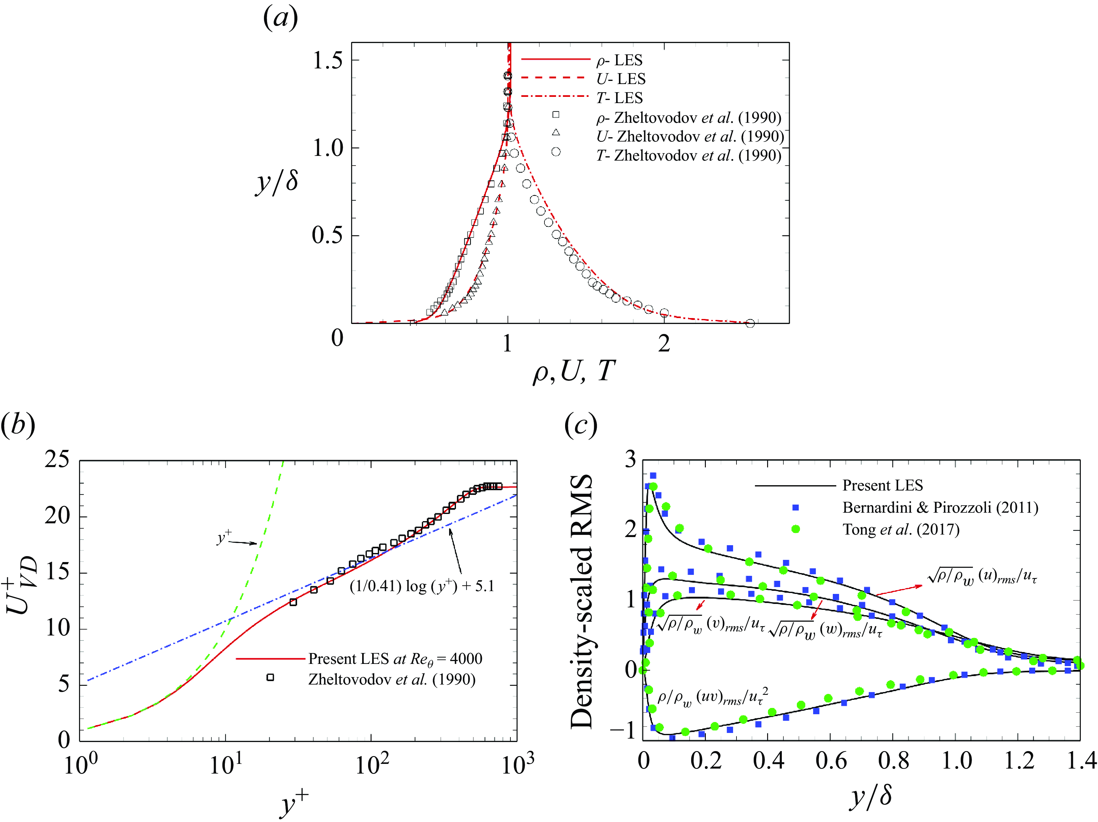
Figure 23. ( $ a$
) Distributions of mean qualities, (
$ a$
) Distributions of mean qualities, ( $ b$
) Van Driest transformed mean velocity profiles, and (
$ b$
) Van Driest transformed mean velocity profiles, and ( $ c$
) comparisons of density-scaled RMS at the reference station
$ c$
) comparisons of density-scaled RMS at the reference station $ x_{0}$
.
$ x_{0}$
.
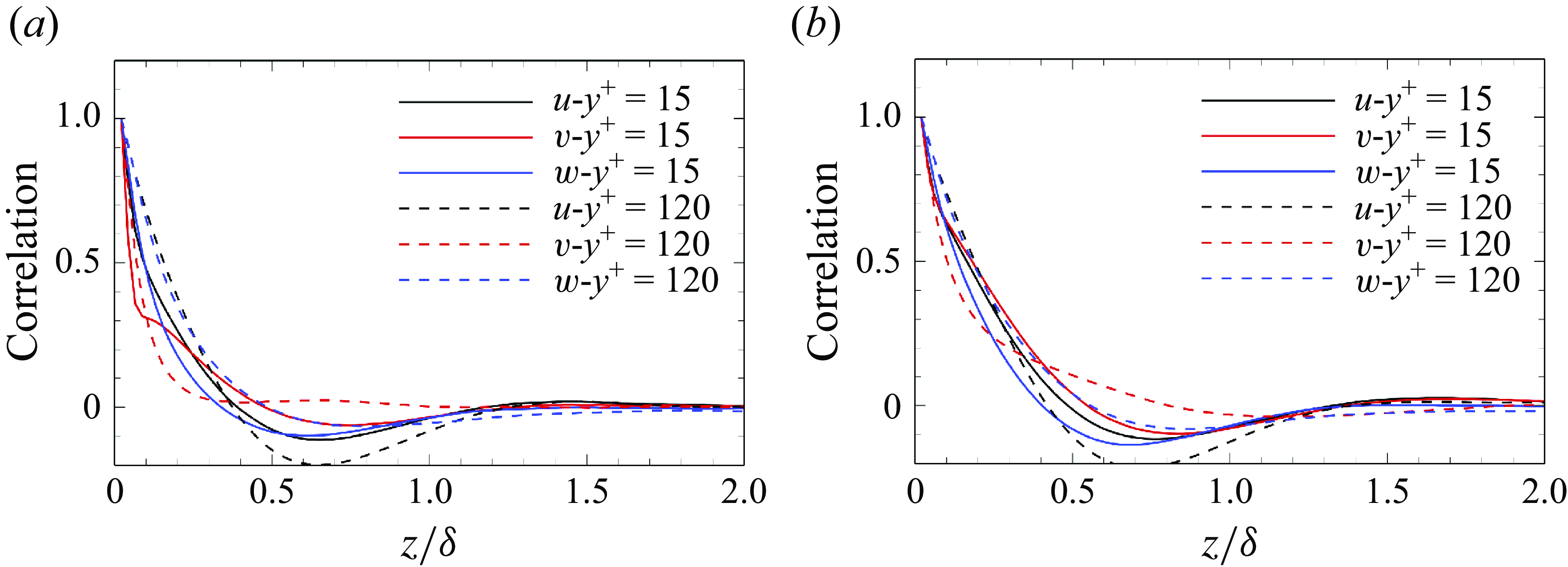
Figure 24. Spanwise correlations at ( $ a$
)
$ a$
) $ \varphi =10^{\circ }$
and (
$ \varphi =10^{\circ }$
and ( $ b$
)
$ b$
) $ \varphi =20^{\circ }$
at two wall-normal stations.
$ \varphi =20^{\circ }$
at two wall-normal stations.
Appendix B. Effect of the forcing location
Figure 25 compares the optimal gains obtained from different forcing locations at $ St=0.036$
. The forcing locations are positioned at 10
$ St=0.036$
. The forcing locations are positioned at 10 $ \delta$
upstream of the concave region and across the entire domain, respectively. The two results show strong agreement, indicating that the optimal response is insensitive to the forcing location. This insensitivity confirms that the dominant amplification mechanism arises from upstream disturbances rather than localised forcing in the concave wall region, consistent with the convective instability characteristics of globally stable flows. Restricting the analysis to upstream disturbances excludes the possibility that large-scale structures may be generated by localised forcing in the curved wall region.
$ \delta$
upstream of the concave region and across the entire domain, respectively. The two results show strong agreement, indicating that the optimal response is insensitive to the forcing location. This insensitivity confirms that the dominant amplification mechanism arises from upstream disturbances rather than localised forcing in the concave wall region, consistent with the convective instability characteristics of globally stable flows. Restricting the analysis to upstream disturbances excludes the possibility that large-scale structures may be generated by localised forcing in the curved wall region.
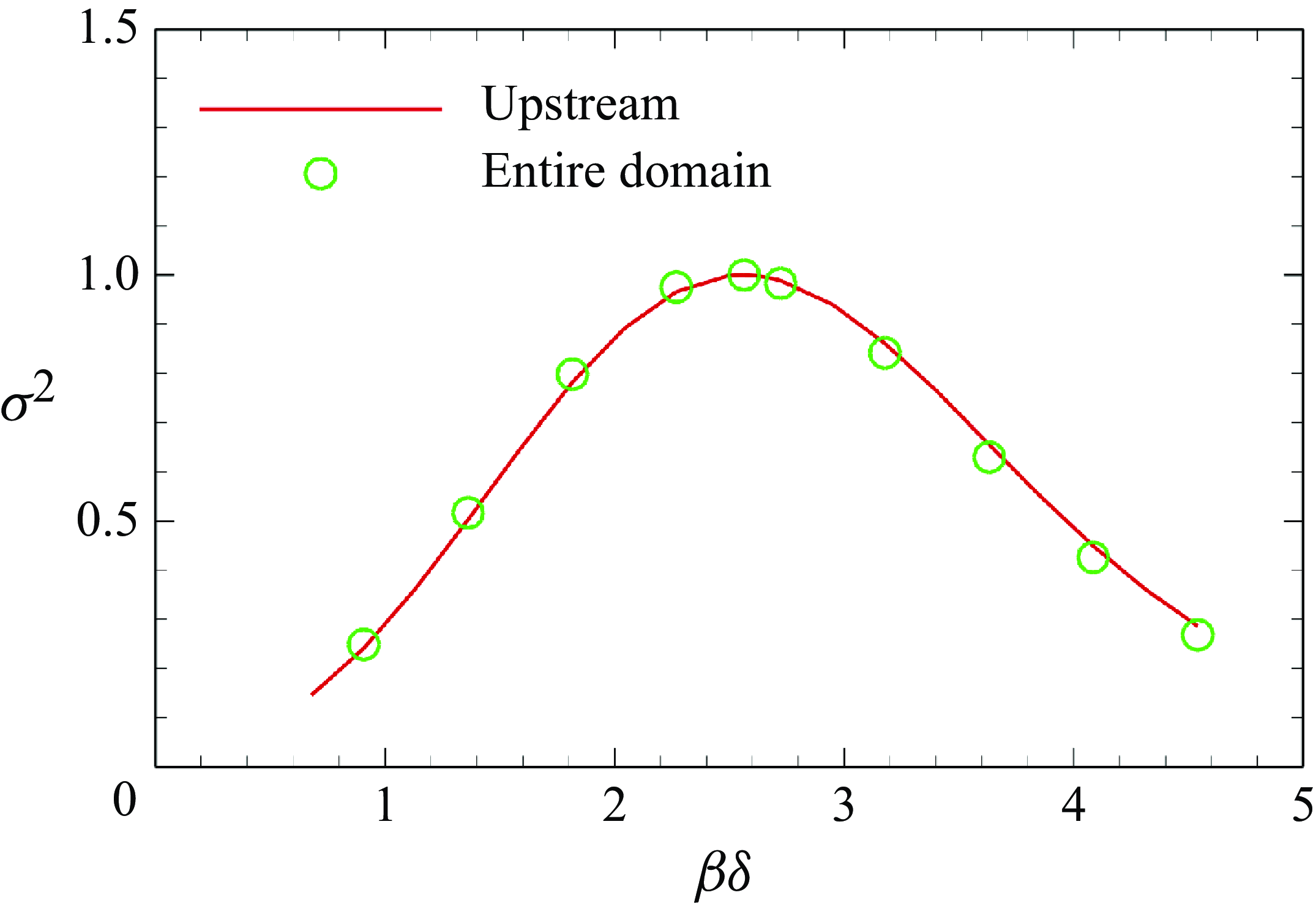
Figure 25. Normalised optimal gains at $ St=0.0361$
as a function of spanwise wavenumbers with different forcing locations.
$ St=0.0361$
as a function of spanwise wavenumbers with different forcing locations.
Appendix C. Convergence analysis
This appendix aims to verify the statistical convergence of the computed POD and SPOD modes. According to Lesshafft et al. (Reference Lesshafft, Semeraro, Jaunet, Cavalieri and Jordan2019) and Abreu et al. (Reference Abreu, Cavalieri, Schlatter, Vinuesa and Henningson2020), the number of samples is a key factor in achieving the convergence of these modes. The correlation coefficient $ \alpha$
between the modes obtained using different subsets is used to analyse the convergence, defined as
$ \alpha$
between the modes obtained using different subsets is used to analyse the convergence, defined as
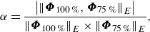 \begin{equation} \alpha =\dfrac {\left | {\| \boldsymbol{\Phi }_{100\, \%}, \boldsymbol{\Phi }_{75\, \%}\| }_{E} \right |}{ {\| \boldsymbol{\Phi }_{100\, \%}\| }_{E} \times {\| \boldsymbol{\Phi }_{75\, \%}\| }_{E} }, \end{equation}
where $ \boldsymbol{\Phi }$
denotes the POD modes or the leading SPOD modes within the frequency band
$ \boldsymbol{\Phi }$
denotes the POD modes or the leading SPOD modes within the frequency band $ St=0.01{-}0.04$
. The subscripts
$ St=0.01{-}0.04$
. The subscripts $ 75\, \%$
and
$ 75\, \%$
and $ 100\, \%$
indicate that the modes are obtained using
$ 100\, \%$
indicate that the modes are obtained using $ 75\, \%$
and
$ 75\, \%$
and $ 100\, \%$
of the total samples, respectively. The
$ 100\, \%$
of the total samples, respectively. The $ 75\, \%$
subset represents either the former or the latter
$ 75\, \%$
subset represents either the former or the latter $ 75\, \%$
of the original dataset. A value of
$ 75\, \%$
of the original dataset. A value of $ \alpha$
close to 1 indicates convergence (Lesshafft et al. Reference Lesshafft, Semeraro, Jaunet, Cavalieri and Jordan2019; Abreu et al. Reference Abreu, Cavalieri, Schlatter, Vinuesa and Henningson2020). Figure 26(
$ \alpha$
close to 1 indicates convergence (Lesshafft et al. Reference Lesshafft, Semeraro, Jaunet, Cavalieri and Jordan2019; Abreu et al. Reference Abreu, Cavalieri, Schlatter, Vinuesa and Henningson2020). Figure 26( $ a$
) shows the correlation coefficients of the first nine POD modes, with
$ a$
) shows the correlation coefficients of the first nine POD modes, with $ \alpha \geqslant 0.93$
for the first two modes. Notably,
$ \alpha \geqslant 0.93$
for the first two modes. Notably, $ \alpha$
is approximately 0.99 for the first mode, which is of particular interest. Figure 26(
$ \alpha$
is approximately 0.99 for the first mode, which is of particular interest. Figure 26( $ b$
) compares the correlation coefficients of the leading SPOD modes of different stations and mid-span plane within
$ b$
) compares the correlation coefficients of the leading SPOD modes of different stations and mid-span plane within $ St=0.01{-}0.04$
. Here,
$ St=0.01{-}0.04$
. Here, $ \alpha \geqslant 0.93$
is maintained for all frequencies. The results from the two 75
$ \alpha \geqslant 0.93$
is maintained for all frequencies. The results from the two 75 $ \, \%$
subsets agree well with those obtained using the whole dataset. Therefore, the POD and SPOD modes are considered converged.
$ \, \%$
subsets agree well with those obtained using the whole dataset. Therefore, the POD and SPOD modes are considered converged.
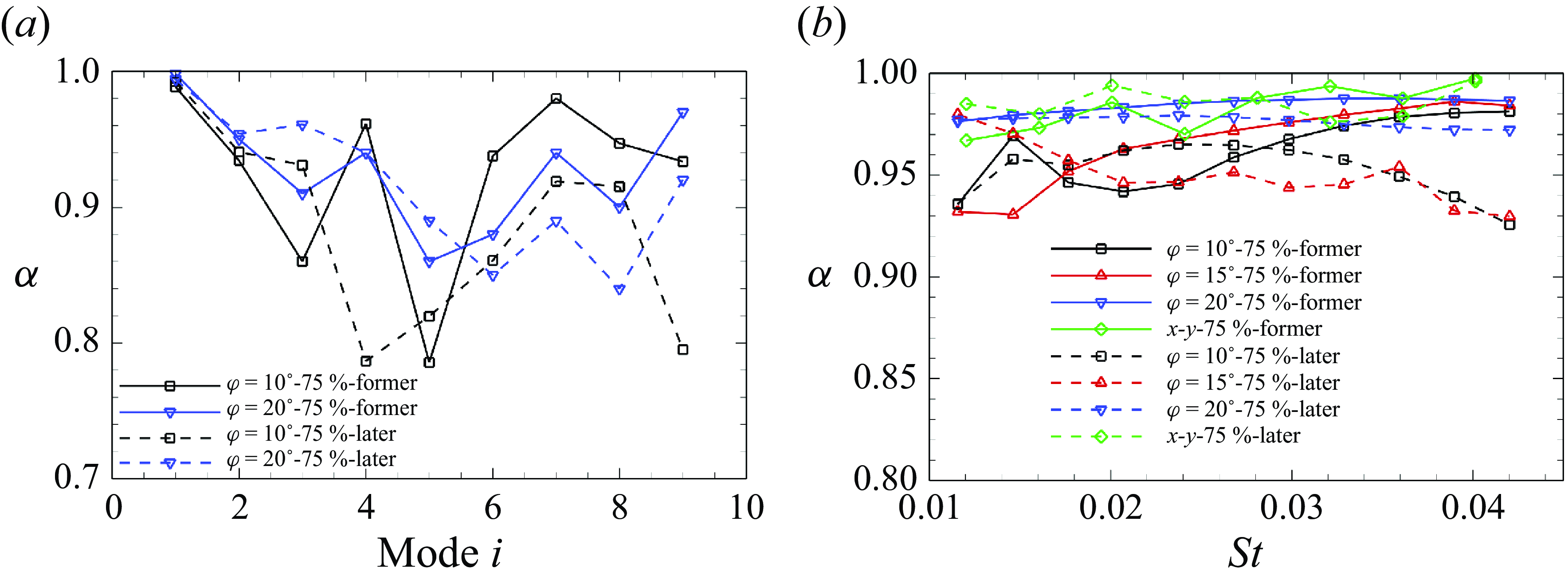
Figure 26. Correlation coefficients $ \alpha$
to quantify the statistical convergence of (
$ \alpha$
to quantify the statistical convergence of ( $ a$
) POD and (
$ a$
) POD and ( $ b$
) SPOD modes.
$ b$
) SPOD modes.


 Open access