


1. Introduction
Understanding sedimentation of deformable, complex-shaped objects is important for various biological systems of particles or cells, for example DNA, polymers or red blood cells (Vologodskii et al. Reference Vologodskii, Crisona, Laurie, Pieranski, Katritch, Dubochet and Stasiak1998; Lo Verso & Likos Reference Lo Verso and Likos2008; Peltomäki & Gompper Reference Peltomäki and Gompper2013; Matsunaga et al. Reference Matsunaga, Imai, Wagner and Ishikawa2016; Waszkiewicz et al. Reference Waszkiewicz, Ranasinghe, Fogg, Catanese, Ekiel-Jeżewska, Lisicki, Demeler, Zechiedrich and Szymczak2023). The gravitational settling of particles of different shapes at the Reynolds number much smaller than unity has been of interest for a long time. The dynamics of various rigid objects have been studied, including conglomerates (Cichocki & Hinsen Reference Cichocki and Hinsen1995), trumbbells (Ekiel-Jeżewska & Wajnryb Reference Ekiel-Jeżewska and Wajnryb2009a ), slender ribbons (Koens & Lauga Reference Koens and Lauga2017), helical ribbons (Huseby et al. Reference Huseby, Gissinger, Candelier, Pujara, Verhille, Mehlig and Voth2025), helices (Palusa et al. Reference Palusa, De Graaf, Brown and Morozov2018), propellers (Makino & Doi Reference Makino and Doi2003), disks (Chajwa, Menon & Ramaswamy Reference Chajwa, Menon and Ramaswamy2019), bent disks (Miara et al. Reference Miara, Vaquero-Stainer, Pihler-Puzović, Heil and Juel2024; Vaquero-Stainer et al. Reference Vaquero-Stainer, Miara, Juel, Pihler-Puzović and Heil2024), Möbius bands (Moreno, Vázquez-Cortés & Fried Reference Moreno, Vázquez-Cortés and Fried2024) and particles of general shapes (Goldfriend et al. Reference Goldfriend, Diamant and Witten2015, Reference Goldfriend, Diamant and Witten2016; Witten & Diamant Reference Witten and Diamant2020; Joshi & Govindarajan Reference Joshi and Govindarajan2025). Depending on the shape, lateral motion, helical trajectories, periodic or quasiperiodic oscillations of singlets and different patterns of hydrodynamic interactions within pairs have been observed.
For elastic objects, the motion can be even more complex, owing to time-dependent shapes. Typical patterns of evolution have been studied for varied elasticity and different shapes, such as filaments (Xu & Nadim Reference Xu and Nadim1994; Cosentino Lagomarsino, Pagonabarraga & Lowe Reference Cosentino Lagomarsino, Pagonabarraga and Lowe2005; Schlagberger & Netz Reference Schlagberger and Netz2005; Manghi et al. Reference Manghi, Schlagberger, Kim and Netz2006; Llopis et al. Reference Llopis, Pagonabarraga, Cosentino Lagomarsino and Lowe2007; Li et al. Reference Li, Manikantan, Saintillan and Spagnolie2013; Saggiorato et al. Reference Saggiorato, Elgeti, Winkler and Gompper2015; Shojaei & Dehghani Reference Shojaei and Dehghani2015; Bukowicki & Ekiel-Jeżewska Reference Bukowicki and Ekiel-Jeżewska2019; du Roure et al. Reference du Roure, Lindner, Nazockdast and Shelley2019; Shashank, Melikhov & Ekiel-Jeżewska Reference Shashank, Melikhov and Ekiel-Jeżewska2023; Melikhov & Ekiel-Jeżewska Reference Melikhov and Ekiel-Jeżewska2024), dumbbells (Bukowicki, Gruca & Ekiel-Jeżewska Reference Bukowicki, Gruca and Ekiel-Jeżewska2015), trumbbells (Bukowicki & Ekiel-Jeżewska Reference Bukowicki and Ekiel-Jeżewska2018), sheets (Miara et al. Reference Miara, Juel, Pihler-Puzovic and Heil2022; Yu & Graham Reference Yu and Graham2024), loops (Gruziel-Słomka et al. Reference Gruziel-Słomka, Kondratiuk, Szymczak and Ekiel-Jeżewska2019; Waszkiewicz, Szymczak & Lisicki Reference Waszkiewicz, Szymczak and Lisicki2021) and knots (Gruziel et al. Reference Gruziel, Thyagarajan, Dietler, Stasiak, Ekiel-Jeżewska and Szymczak2018).
Until now, most of papers on sedimenting deformable objects focused on the dynamics of moderately elastic filaments (Xu & Nadim Reference Xu and Nadim1994; Cosentino Lagomarsino et al. Reference Cosentino Lagomarsino, Pagonabarraga and Lowe2005; Schlagberger & Netz Reference Schlagberger and Netz2005; Manghi et al. Reference Manghi, Schlagberger, Kim and Netz2006; Llopis et al. Reference Llopis, Pagonabarraga, Cosentino Lagomarsino and Lowe2007; Li et al. Reference Li, Manikantan, Saintillan and Spagnolie2013; Shojaei & Dehghani Reference Shojaei and Dehghani2015; Bukowicki & Ekiel-Jeżewska Reference Bukowicki and Ekiel-Jeżewska2019; du Roure et al. Reference du Roure, Lindner, Nazockdast and Shelley2019). The main finding was the existence of a stable, stationary, planar, vertical configuration. The dependence of its U-like shape on the bending stiffness was determined. Recently, very different, rich dynamics of highly elastic filaments have been reported (Saggiorato et al. Reference Saggiorato, Elgeti, Winkler and Gompper2015; Shashank et al. Reference Shashank, Melikhov and Ekiel-Jeżewska2023; Melikhov & Ekiel-Jeżewska Reference Melikhov and Ekiel-Jeżewska2024). In these studies, the ends of the filament can move relative to each other. However, it is also interesting to investigate the dynamics of highly elastic loops.
In this work, we show that a circular non-horizontal elastic loop settling under gravity in a viscous fluid at Reynolds number much smaller than unity is not a stationary configuration. We focus on the analysis of other stationary configurations, and other attracting dynamical modes of highly elastic loops settling under gravity in a viscous fluid at Reynolds number much smaller than unity. We extend the previous results (Gruziel-Słomka et al. Reference Gruziel-Słomka, Kondratiuk, Szymczak and Ekiel-Jeżewska2019; Waszkiewicz et al. Reference Waszkiewicz, Szymczak and Lisicki2021) by evaluating the characteristic time scales and velocities (what is essential for separating different modes or applying them), and finding numerically bifurcations between the modes at critical values of the bending stiffness (what is a prerequisite to understanding the nature of the different modes). We also find a new mode.
The plan of the paper is as follows. The theoretical model, its numerical implementation and its parameters are presented in § 2. Properties of the dynamical modes reached from inclined planar and non-planar initial configurations for different values of the elasto-gravitation number are analysed in §§ 3 and 4, respectively. Characteristic time scales and loop velocities for different attracting modes are determined in § 5. Discussion and conclusions are presented in § 6.
2. Methodology
2.1. Model of elastic loops and their dynamics
The bead–spring model is used to represent an elastic fibre of length ${\mathcal{L}}$
and diameter of the circular cross-section
${\mathcal{L}}$
and diameter of the circular cross-section $d$
. The fibre is closed and it forms a loop. It is modelled as a chain of
$d$
. The fibre is closed and it forms a loop. It is modelled as a chain of $N$
identical non-deformable spherical beads
$N$
identical non-deformable spherical beads $N$
of diameter
$N$
of diameter $d$
. Position of the centre of the ith bead is denoted as
$d$
. Position of the centre of the ith bead is denoted as $\boldsymbol{r}_i$
, for
$\boldsymbol{r}_i$
, for $i=1,\ldots ,N$
. Consecutive beads interact with each other by the finitely extensible nonlinear elastic (FENE) spring potential energy (Warner Reference Warner1972; Bird, Armstrong & Hassager Reference Bird, Armstrong and Hassager1977),
$i=1,\ldots ,N$
. Consecutive beads interact with each other by the finitely extensible nonlinear elastic (FENE) spring potential energy (Warner Reference Warner1972; Bird, Armstrong & Hassager Reference Bird, Armstrong and Hassager1977),
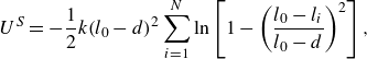 \begin{equation} U^{S} = - \frac {1}{2} k (l_{0}-d)^{2} \sum _{i=1}^{N}\ln \left [ {1 - \left ( \frac {l_{0}-l_{i}}{l_{0}-d} \right )^{2}} \right ], \end{equation}
where $l_i=|\boldsymbol{r}_{i+1}-\boldsymbol{r}_{i}|$
for
$l_i=|\boldsymbol{r}_{i+1}-\boldsymbol{r}_{i}|$
for $i=1,\ldots ,N-1$
,
$i=1,\ldots ,N-1$
, $l_N=|\boldsymbol{r}_{1}-\boldsymbol{r}_{N}|$
,
$l_N=|\boldsymbol{r}_{1}-\boldsymbol{r}_{N}|$
, $l_{0}$
is the equilibrium distance between beads centres and
$l_{0}$
is the equilibrium distance between beads centres and $k$
is a spring constant.
$k$
is a spring constant.
The finitely extensible nonlinear elastic (FENE) spring potential allows for precise treatment of the dynamics of very close bead surfaces, preventing spurious overlaps. The choice of a small value $l_{0}=1.01d$
leads to small time-dependent gaps between the surfaces of the consecutive beads. Therefore, the loops can stretch a bit but are almost inextensible. The fibre aspect ratio is well-approximated by the number of beads,
$l_{0}=1.01d$
leads to small time-dependent gaps between the surfaces of the consecutive beads. Therefore, the loops can stretch a bit but are almost inextensible. The fibre aspect ratio is well-approximated by the number of beads, ${\mathcal {L}}/d \approx N$
.
${\mathcal {L}}/d \approx N$
.
In addition, there are also bending forces. It is assumed that each triplet of the consecutive beads is straight at the elastic equilibrium, and it harmonically resists bending, leading to the following bending potential energy of the whole loop,
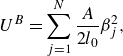 \begin{equation} U^{B}= \sum _{j=1}^{N} \frac {A}{2 l_{0}} \beta _{j}^2, \end{equation}
where $A$
is the bending stiffness, and
$A$
is the bending stiffness, and $\beta _{i}$
is the bending angle between the consecutive bonds, with
$\beta _{i}$
is the bending angle between the consecutive bonds, with $\cos \beta _i\!=\!({\boldsymbol{r}}_i\!-\!{\boldsymbol{r}}_{i-1})\cdot ({\boldsymbol{r}}_{i+1}\!-\!{\boldsymbol{r}}_{i})/(l_{i-1} l_{i})$
for
$\cos \beta _i\!=\!({\boldsymbol{r}}_i\!-\!{\boldsymbol{r}}_{i-1})\cdot ({\boldsymbol{r}}_{i+1}\!-\!{\boldsymbol{r}}_{i})/(l_{i-1} l_{i})$
for $i=2,\ldots ,N-1$
,
$i=2,\ldots ,N-1$
, $\cos \beta _1=(\boldsymbol{r}_{1}-\boldsymbol{r}_{N})\cdot (\boldsymbol{r}_{2}-\boldsymbol{r}_{1})/(l_{N} l_{1})$
and
$\cos \beta _1=(\boldsymbol{r}_{1}-\boldsymbol{r}_{N})\cdot (\boldsymbol{r}_{2}-\boldsymbol{r}_{1})/(l_{N} l_{1})$
and $\cos \beta _N=(\boldsymbol{r}_{N}-\boldsymbol{r}_{N-1})\cdot (\boldsymbol{r}_{1}-\boldsymbol{r}_{N})/(l_{N-1} l_{N})$
. For highly elastic fibres, the harmonic bending potential energy (MacKerell et al. Reference MacKerell1998; Storm & Nelson Reference Storm and Nelson2003; Frenkel & Smit Reference Frenkel and Smit2023), used in this work, is more realistic than the Kratky–Porod potential energy (Schlagberger & Netz Reference Schlagberger and Netz2005; Manghi et al. Reference Manghi, Schlagberger, Kim and Netz2006; Llopis et al. Reference Llopis, Pagonabarraga, Cosentino Lagomarsino and Lowe2007; Saggiorato et al. Reference Saggiorato, Elgeti, Winkler and Gompper2015; Marchetti et al. Reference Marchetti, Raspa, Lindner, du Roure, Bergougnoux, Guazzelli and Duprat2018). The reason is that for larger bending angles (as it happens for highly elastic fibres), the Kratky–Porod potential may lead to spurious dynamics (Bukowicki & Ekiel-Jeżewska Reference Bukowicki and Ekiel-Jeżewska2018).
$\cos \beta _N=(\boldsymbol{r}_{N}-\boldsymbol{r}_{N-1})\cdot (\boldsymbol{r}_{1}-\boldsymbol{r}_{N})/(l_{N-1} l_{N})$
. For highly elastic fibres, the harmonic bending potential energy (MacKerell et al. Reference MacKerell1998; Storm & Nelson Reference Storm and Nelson2003; Frenkel & Smit Reference Frenkel and Smit2023), used in this work, is more realistic than the Kratky–Porod potential energy (Schlagberger & Netz Reference Schlagberger and Netz2005; Manghi et al. Reference Manghi, Schlagberger, Kim and Netz2006; Llopis et al. Reference Llopis, Pagonabarraga, Cosentino Lagomarsino and Lowe2007; Saggiorato et al. Reference Saggiorato, Elgeti, Winkler and Gompper2015; Marchetti et al. Reference Marchetti, Raspa, Lindner, du Roure, Bergougnoux, Guazzelli and Duprat2018). The reason is that for larger bending angles (as it happens for highly elastic fibres), the Kratky–Porod potential may lead to spurious dynamics (Bukowicki & Ekiel-Jeżewska Reference Bukowicki and Ekiel-Jeżewska2018).
The bending stiffness $A$
is proportional to the Young’s modulus
$A$
is proportional to the Young’s modulus $E_{Y}$
by the model of an elastic cylinder of diameter
$E_{Y}$
by the model of an elastic cylinder of diameter $d$
(Bukowicki & Ekiel-Jeżewska Reference Bukowicki and Ekiel-Jeżewska2018; Bukowicki & Ekiel-Jeżewska Reference Bukowicki and Ekiel-Jeżewska2019),
$d$
(Bukowicki & Ekiel-Jeżewska Reference Bukowicki and Ekiel-Jeżewska2018; Bukowicki & Ekiel-Jeżewska Reference Bukowicki and Ekiel-Jeżewska2019),
 \begin{equation} A = \frac {E_Y \pi d^4}{64}. \end{equation}
The same elastic model is applied to the spring constant $k$
, and therefore the spring constant
$k$
, and therefore the spring constant $k$
is linked to the bending stiffness
$k$
is linked to the bending stiffness $A$
by the relation (Bukowicki & Ekiel-Jeżewska Reference Bukowicki and Ekiel-Jeżewska2018)
$A$
by the relation (Bukowicki & Ekiel-Jeżewska Reference Bukowicki and Ekiel-Jeżewska2018)
 \begin{equation} A = \frac {k d^{2} l_{0}}{ 16}. \end{equation}
The potential energies (2.1)–(2.2) result in the following expression for the elastic force onto the $j$
th bead, for
$j$
th bead, for $j=1,\ldots ,N$
:
$j=1,\ldots ,N$
:
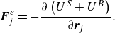 \begin{equation} {\boldsymbol{F}}^{e}_{\! j} = - \frac {\partial \left ( U^{S} + U^{B} \right )}{\partial {\boldsymbol{r}}_{\! j}}. \end{equation}
There is also a constant gravitational force, corrected for buoyancy, which acts on each bead $j$
along the
$j$
along the $z$
-axis,
$z$
-axis,
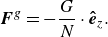 \begin{equation} \boldsymbol{F}^g = - \frac {G}{N} \cdot \boldsymbol{ \hat {e} }_z. \end{equation}
Here, $G$
is the total gravitational force on the whole loop, and
$G$
is the total gravitational force on the whole loop, and $\boldsymbol{ \hat {e} }_z$
is the unit vector along the
$\boldsymbol{ \hat {e} }_z$
is the unit vector along the $z$
-axis.
$z$
-axis.
We restrict ourselves to the systems with the Reynolds number much smaller than unity. Therefore, the fluid flow obeys the Stokes equations, and the bead velocities, $\dot {\boldsymbol{r}}_{i}$
, depend linearly on the elastic and gravitational forces exerted on the beads
$\dot {\boldsymbol{r}}_{i}$
, depend linearly on the elastic and gravitational forces exerted on the beads $j$
. The dynamics of the positions of the bead centres
$j$
. The dynamics of the positions of the bead centres $\boldsymbol{r}_i$
,
$\boldsymbol{r}_i$
, $i=1,\ldots ,N$
, satisfy the set of the first-order ordinary differential equations,
$i=1,\ldots ,N$
, satisfy the set of the first-order ordinary differential equations,
 \begin{equation} \dot {\boldsymbol{r}}_{i} = \sum _{j=1}^{N} \boldsymbol{\mu }_{ij}(\boldsymbol{r}_1,\ldots ,\boldsymbol{r}_N) \cdot \left ( \boldsymbol{F}_{\! j}^e + \boldsymbol{F}^g \right ). \end{equation}
The $3\times3$
mobility matrices
$3\times3$
mobility matrices $\boldsymbol{\mu }_{ij}(\boldsymbol{r}_1,\ldots ,\boldsymbol{r}_N)$
, for
$\boldsymbol{\mu }_{ij}(\boldsymbol{r}_1,\ldots ,\boldsymbol{r}_N)$
, for $i,j=1,\ldots ,N$
, depend on the time-dependent positions of all the bead centres. They are calculated by the multipole expansion of the solutions to the Stokes equations, corrected for lubrication to speed up the expansion convergence (Felderhof Reference Felderhof1988; Cichocki et al. Reference Cichocki, Felderhof, Hinsen, Wajnryb and Bławzdziewicz1994, Reference Cichocki, Ekiel-Jeżewska and Wajnryb1999). The lubrication correction between all the bead pairs (also non-neighbouring beads) is always switched on in the simulations.
$i,j=1,\ldots ,N$
, depend on the time-dependent positions of all the bead centres. They are calculated by the multipole expansion of the solutions to the Stokes equations, corrected for lubrication to speed up the expansion convergence (Felderhof Reference Felderhof1988; Cichocki et al. Reference Cichocki, Felderhof, Hinsen, Wajnryb and Bławzdziewicz1994, Reference Cichocki, Ekiel-Jeżewska and Wajnryb1999). The lubrication correction between all the bead pairs (also non-neighbouring beads) is always switched on in the simulations.
The elastic forces $\boldsymbol{F}_{\! j}^e$
depend only on the time-dependent positions
$\boldsymbol{F}_{\! j}^e$
depend only on the time-dependent positions $\boldsymbol{r}_i(t)$
of all the bead centres
$\boldsymbol{r}_i(t)$
of all the bead centres $i=1,\ldots ,N$
. Therefore, (2.7) can be solved for any initial positions of the bead centres,
$i=1,\ldots ,N$
. Therefore, (2.7) can be solved for any initial positions of the bead centres, $\boldsymbol{r}_i(0)$
, for
$\boldsymbol{r}_i(0)$
, for $i=1,\ldots ,N$
, no matter what the angular velocity
$i=1,\ldots ,N$
, no matter what the angular velocity $\boldsymbol{\Omega }_i(t)$
of each bead.
$\boldsymbol{\Omega }_i(t)$
of each bead.
In the following, we choose $G/N$
as the force unit, and adopt the following units for the length, time and translational and rotational velocities:
$G/N$
as the force unit, and adopt the following units for the length, time and translational and rotational velocities:
 \begin{equation} d, \quad \tau _{b}= \frac {\pi \eta d^2N}{G}, \quad v_{b}=\frac {d}{\tau _{b}}=\frac {G}{\pi \eta d N}, \quad \omega _{b}=\frac {1}{\tau _{b}}=\frac {G}{\pi \eta d^2N}. \end{equation}
From now on, we redefine the symbols used previously to mean the corresponding dimensionless quantities.
2.2. Simulations, parameters and variables
The precise numerical code HYDROMULTIPOLE (Cichocki, Ekiel-Jeżewska & Wajnryb Reference Cichocki, Ekiel-Jeżewska and Wajnryb1999; Ekiel-Jeżewska & Wajnryb Reference Ekiel-Jeżewska, Wajnryb, Feuillebois and Sellier2009b
), based on multipole expansion of solutions to the Stokes equations, corrected for lubrication (Cichocki et al. Reference Cichocki, Ekiel-Jeżewska and Wajnryb1999), is used to evaluate the mobility matrices $\boldsymbol{\mu }_{ij}(\boldsymbol{r}_1,\ldots ,\boldsymbol{r}_N)$
for the elastic fibre made of
$\boldsymbol{\mu }_{ij}(\boldsymbol{r}_1,\ldots ,\boldsymbol{r}_N)$
for the elastic fibre made of $N=36$
beads and solve the dynamics in (2.7). The lubrication correction is applied to the relative motions of each pair of beads. The multipole truncation order
$N=36$
beads and solve the dynamics in (2.7). The lubrication correction is applied to the relative motions of each pair of beads. The multipole truncation order $L=2$
is taken in these computations. An adaptive fourth-order Runge–Kutta method was employed with the limit of the maximum timestep set to
$L=2$
is taken in these computations. An adaptive fourth-order Runge–Kutta method was employed with the limit of the maximum timestep set to $0.5$
. The majority of the simulations were performed until
$0.5$
. The majority of the simulations were performed until $t=88\,000$
. A few selected simulations were run for longer times.
$t=88\,000$
. A few selected simulations were run for longer times.
Following Cosentino Lagomarsino et al. Reference Cosentino Lagomarsino, Pagonabarraga and Lowe2005, Llopis et al. Reference Llopis, Pagonabarraga, Cosentino Lagomarsino and Lowe2007, Saggiorato et al. Reference Saggiorato, Elgeti, Winkler and Gompper2015, Bukowicki & Ekiel-Jeżewska Reference Bukowicki and Ekiel-Jeżewska2018, Marchetti et al. Reference Marchetti, Raspa, Lindner, du Roure, Bergougnoux, Guazzelli and Duprat2018, and Bukowicki & Ekiel-Jeżewska Reference Bukowicki and Ekiel-Jeżewska2019, we introduce in this work the elasto-gravitation number, $B$
, that is a ratio of the gravitational and bending forces acting on the loop,
$B$
, that is a ratio of the gravitational and bending forces acting on the loop,
 \begin{equation} B = \dfrac {{\mathcal {L}}^2 G}{A}. \end{equation}
In our model, the fibre aspect ratio ${\mathcal {L}}/d \approx N$
, and therefore
${\mathcal {L}}/d \approx N$
, and therefore $B \approx {N^2 d^2 G}/{A}$
.
$B \approx {N^2 d^2 G}/{A}$
.
In the simulations, the number of beads in the loop is fixed, $N=36$
. The value of
$N=36$
. The value of $B$
is varied in the range
$B$
is varied in the range $1000 \le B \le 40\,000$
. Within the considered range of values of the elasto-gravitation number, the moderately elastic loops, with smaller values of
$1000 \le B \le 40\,000$
. Within the considered range of values of the elasto-gravitation number, the moderately elastic loops, with smaller values of $B$
, deform from a circle only slightly. However, highly elastic loops, with larger values of
$B$
, deform from a circle only slightly. However, highly elastic loops, with larger values of $B$
, deform significantly out of a plane.
$B$
, deform significantly out of a plane.
To study the time evolution of the loop orientation, we evaluate the time-dependent gyration tensor (Mattice & Suter Reference Mattice and Suter1994),
 \begin{equation} {S}_{\alpha \beta } = \frac {1}{N}\sum \limits _{j=1}^{N} r'_{j\alpha } r'_{j\beta }, \end{equation}
where $\alpha = x, y, z,\;\beta = x, y, z$
and
$\alpha = x, y, z,\;\beta = x, y, z$
and ${\boldsymbol{r}}'_{\! j}=(r'_{jx},r'_{jy},r'_{jz})$
is the position of
${\boldsymbol{r}}'_{\! j}=(r'_{jx},r'_{jy},r'_{jz})$
is the position of $j$
th bead centre in the centre-of-mass reference frame,
$j$
th bead centre in the centre-of-mass reference frame, ${\boldsymbol{r}}'_{\! j}={\boldsymbol{r}}_{\! j}-\boldsymbol{r}_{CM}$
, with the centre-of-mass position
${\boldsymbol{r}}'_{\! j}={\boldsymbol{r}}_{\! j}-\boldsymbol{r}_{CM}$
, with the centre-of-mass position
 \begin{equation} {\boldsymbol{r}}_{CM}\equiv \frac {1}{N}\sum _{i=1}^N \boldsymbol{r}_i=(x_{CM},y_{CM},z_{CM}). \end{equation}
We find the eigenvalues and eigenvectors of the gyration tensor defined in (2.10). We select the unit eigenvector associated with the smallest eigenvalue and denote it as $\boldsymbol{n}$
. The unit vector
$\boldsymbol{n}$
. The unit vector $\boldsymbol{n}$
is used to provide information about the orientation of the loop. For example, in the case of a circular flat loop with its centre at the origin of the coordinate system, the unit vector
$\boldsymbol{n}$
is used to provide information about the orientation of the loop. For example, in the case of a circular flat loop with its centre at the origin of the coordinate system, the unit vector $\boldsymbol{n}$
is perpendicular to the plane of the loop, and it lies on the loop rotational symmetry axis.
$\boldsymbol{n}$
is perpendicular to the plane of the loop, and it lies on the loop rotational symmetry axis.
Expressing $\boldsymbol{n}$
in spherical coordinates with the polar angle
$\boldsymbol{n}$
in spherical coordinates with the polar angle $\theta$
that it makes with the vertical axis
$\theta$
that it makes with the vertical axis $z$
(antiparallel to gravity), and the azimuthal angle
$z$
(antiparallel to gravity), and the azimuthal angle $\phi$
that its projection onto the
$\phi$
that its projection onto the $xy$
-plane makes with the
$xy$
-plane makes with the $x$
-axis,
$x$
-axis,
 \begin{equation} \boldsymbol{n} = \begin{pmatrix} \sin \theta \cos \phi , \sin \theta \sin \phi , \cos \theta \end{pmatrix} \end{equation}
we will monitor dependencies of $\theta$
and
$\theta$
and $\phi$
on time, and we will use them to help us to characterise the dynamical modes.
$\phi$
on time, and we will use them to help us to characterise the dynamical modes.
3. The dynamical modes reached from an inclined planar initial configuration
3.1. Outline
In this section, we present the majority of our simulations. We focus on a flat inclined circle as the initial configuration, similarly as in Gruziel-Słomka et al. (Reference Gruziel-Słomka, Kondratiuk, Szymczak and Ekiel-Jeżewska2019). Typically, $\theta (t=0)=16^{\circ }$
for highly elastic loops, and
$\theta (t=0)=16^{\circ }$
for highly elastic loops, and $\theta (t=0)=80^{\circ }$
for some moderately elastic loops. A few simulations performed with curved initial configurations will be presented in § 4.
$\theta (t=0)=80^{\circ }$
for some moderately elastic loops. A few simulations performed with curved initial configurations will be presented in § 4.
We find numerically that a highly elastic loop, after a relatively long time, reaches a certain dynamical mode and remains in this mode for a very long time until the end of the simulations. For a given initial configuration, the type of the mode reached depends on a value of the elasto-gravitation number $B$
. We observe the following dynamical modes: vertical (V), tilted (T), rocking (R), gyrating-rocking-tank-treading (GRTT), frozen rotating (FR), tank-treading (TT), swinging (S) and flapping (F).
$B$
. We observe the following dynamical modes: vertical (V), tilted (T), rocking (R), gyrating-rocking-tank-treading (GRTT), frozen rotating (FR), tank-treading (TT), swinging (S) and flapping (F).
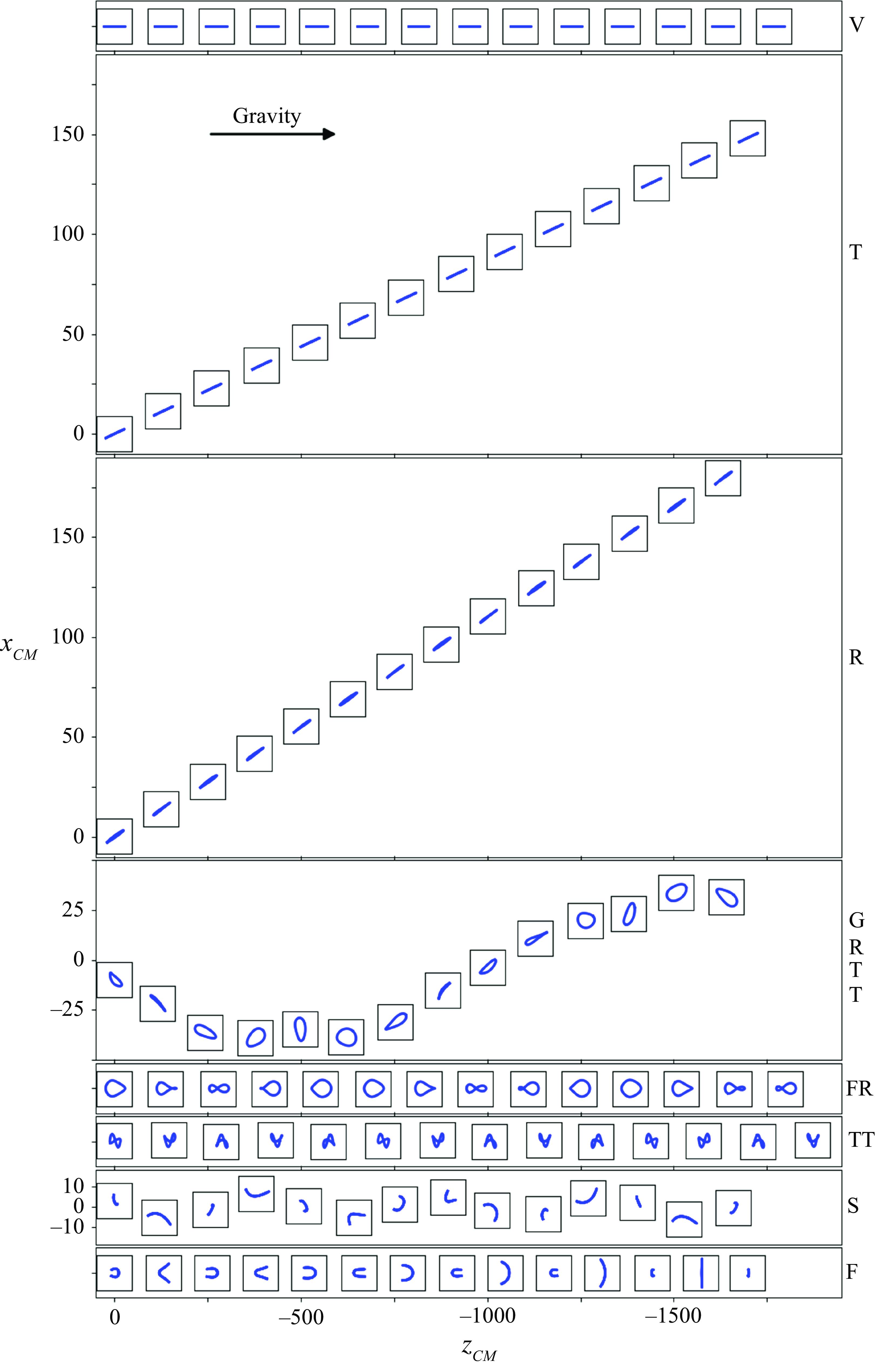
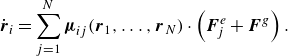
Figure 1. The time sequence of the loop shapes and their centre-of-mass positions at the $(x,z)$
projection for different attracting modes: vertical (V), tilted (T), rocking (R), gyrating-rocking-tank-treading (GRTT), frozen rotating (FR), tank-treading (TT), swinging (S), and flapping (F), for
$(x,z)$
projection for different attracting modes: vertical (V), tilted (T), rocking (R), gyrating-rocking-tank-treading (GRTT), frozen rotating (FR), tank-treading (TT), swinging (S), and flapping (F), for $B=6030, 7714, 14\,098, 17\,422, 22\,497, 34\,843, 35\,993$
and
$B=6030, 7714, 14\,098, 17\,422, 22\,497, 34\,843, 35\,993$
and $40\,000$
, respectively. The time step between the neighbouring insets is
$40\,000$
, respectively. The time step between the neighbouring insets is $\Delta t = 83$
, and the total time
$\Delta t = 83$
, and the total time $t=1079$
. Each inset represents the loop shape in a square of
$t=1079$
. Each inset represents the loop shape in a square of $10d$
by
$10d$
by $10d$
. The centre of each inset is positioned at the centre of mass of the loop at that particular time.
$10d$
. The centre of each inset is positioned at the centre of mass of the loop at that particular time.
The snapshots of the sedimenting elastic fibres ( $xz$
projection), separated by the same time interval
$xz$
projection), separated by the same time interval $\Delta t=83$
, are presented in figure 1, accompanied by the Supplementary movies. The evolution of the shapes in the vertical, tilted, frozen rotating, tank-treading, swinging and flapping modes observed in this work is qualitatively similar to that reported earlier in Gruziel-Słomka et al. (Reference Gruziel-Słomka, Kondratiuk, Szymczak and Ekiel-Jeżewska2019), where a numerical study was performed using the Rotne–Prager method. This work describes two additional modes: rocking and gyrating-rocking-tank-treading. The rocking mode might be the same as the tilted swinging mode in Gruziel-Słomka et al. (Reference Gruziel-Słomka, Kondratiuk, Szymczak and Ekiel-Jeżewska2019), but the shape evolution of the tilted swinging mode was not provided there. (The evolution of shapes in the rocking mode is essentially different from that in the swinging mode.)
$\Delta t=83$
, are presented in figure 1, accompanied by the Supplementary movies. The evolution of the shapes in the vertical, tilted, frozen rotating, tank-treading, swinging and flapping modes observed in this work is qualitatively similar to that reported earlier in Gruziel-Słomka et al. (Reference Gruziel-Słomka, Kondratiuk, Szymczak and Ekiel-Jeżewska2019), where a numerical study was performed using the Rotne–Prager method. This work describes two additional modes: rocking and gyrating-rocking-tank-treading. The rocking mode might be the same as the tilted swinging mode in Gruziel-Słomka et al. (Reference Gruziel-Słomka, Kondratiuk, Szymczak and Ekiel-Jeżewska2019), but the shape evolution of the tilted swinging mode was not provided there. (The evolution of shapes in the rocking mode is essentially different from that in the swinging mode.)
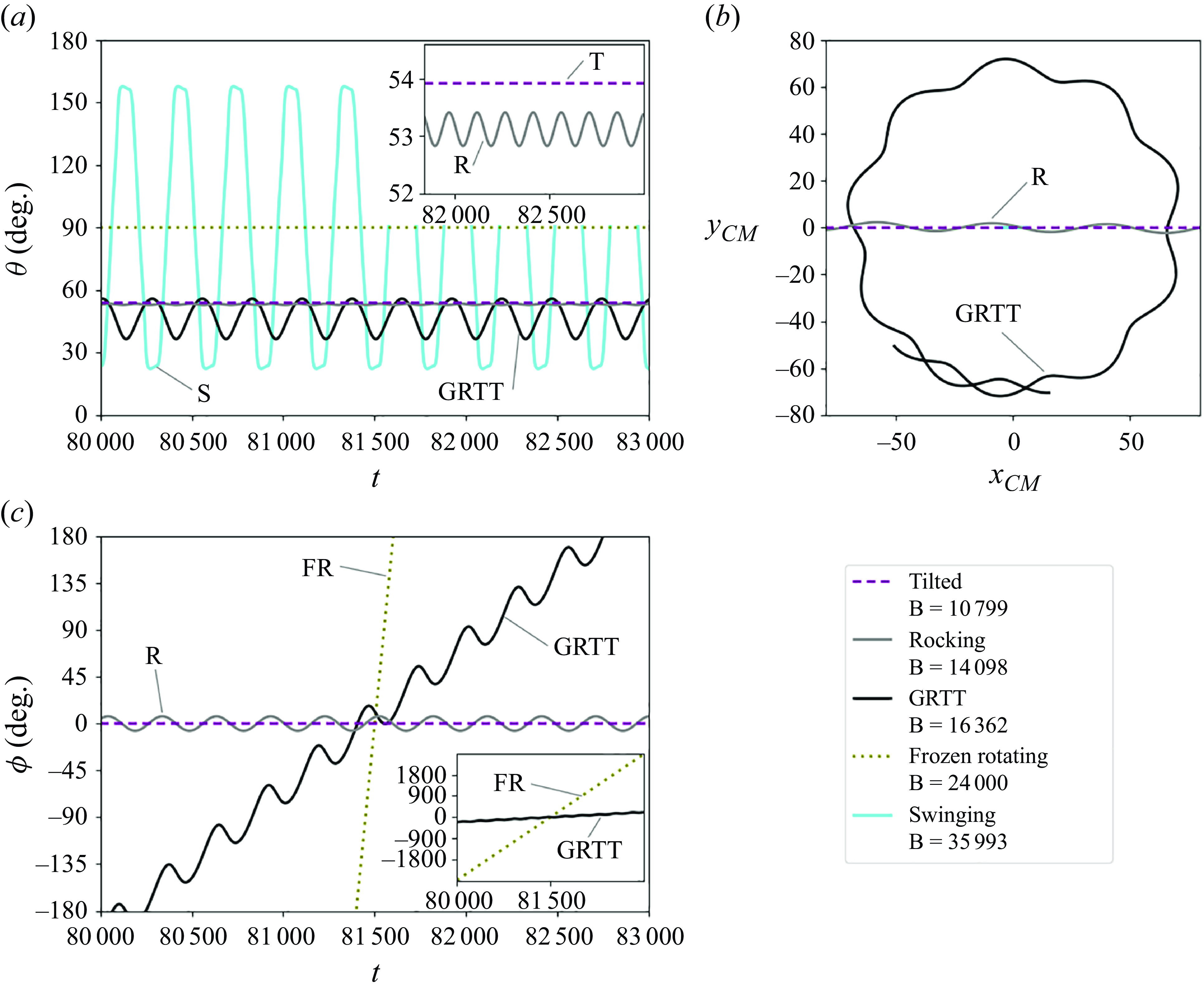
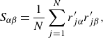
Figure 2. Different attracting dynamical modes: the time dependence of (a) polar angle $\theta$
and (c) azimuthal angle
$\theta$
and (c) azimuthal angle $\phi$
, together with (b) horizontal projections of the centre-of-mass trajectories. In (b), the ranges of times are
$\phi$
, together with (b) horizontal projections of the centre-of-mass trajectories. In (b), the ranges of times are $963$
for the tilted,
$963$
for the tilted, $968$
for the rocking and
$968$
for the rocking and $3000$
for the GRTT modes. In (b), for the swinging mode, the centre-of-mass of the loop oscillates on the line
$3000$
for the GRTT modes. In (b), for the swinging mode, the centre-of-mass of the loop oscillates on the line $y_{CM} \!=\! 0$
between
$y_{CM} \!=\! 0$
between $-7 \le x_{CM} \le 7$
, which it covers during time period of
$-7 \le x_{CM} \le 7$
, which it covers during time period of $303$
; for the frozen rotating mode,
$303$
; for the frozen rotating mode, $x_{CM}\! = \!0$
and
$x_{CM}\! = \!0$
and $y_{CM}\! = \!0$
.
$y_{CM}\! = \!0$
.
The important new input of the present paper is the evaluation of the characteristic time scales and velocities for all the attracting dynamical modes. A qualitative comparison of the mean velocities can be found in figure 1, where we show the motion of the fibre centre-of-mass. Each snapshot of the fibre shape (drawn to scale) is centred at the loop centre-of-mass position $(x_{CM}, z_{CM})$
at the corresponding time instant. The time of the recorded motion,
$(x_{CM}, z_{CM})$
at the corresponding time instant. The time of the recorded motion, $t=1079$
, is the same for all the modes. By comparing the last vertical coordinate
$t=1079$
, is the same for all the modes. By comparing the last vertical coordinate $z_{CM}$
, we clearly see that the mean sedimentation speed for different modes is different; the settling of the fibre in the TT mode is the fastest. Also, by looking at the last horizontal coordinate
$z_{CM}$
, we clearly see that the mean sedimentation speed for different modes is different; the settling of the fibre in the TT mode is the fastest. Also, by looking at the last horizontal coordinate $x_{CM}$
, it is clear that the fibres in the tilted and rocking modes move laterally, and their horizontal displacement can be as large as around 10 % of the vertical one.
$x_{CM}$
, it is clear that the fibres in the tilted and rocking modes move laterally, and their horizontal displacement can be as large as around 10 % of the vertical one.
For different modes, we also analyse the time dependence of the loop three-dimensional (3-D) orientation, $\theta$
,
$\theta$
, $\phi$
and its 3-D centre-of-mass motion,
$\phi$
and its 3-D centre-of-mass motion, $(x_{CM},y_{CM},z_{CM})$
. The exemplary comparison of
$(x_{CM},y_{CM},z_{CM})$
. The exemplary comparison of $\theta (t)$
,
$\theta (t)$
, $\phi (t)$
and
$\phi (t)$
and $y_{CM}(x_{CM})$
for different attracting modes is presented in figure 2. Here, we do not include the vertical mode (with
$y_{CM}(x_{CM})$
for different attracting modes is presented in figure 2. Here, we do not include the vertical mode (with $\theta =90^\circ$
,
$\theta =90^\circ$
, $\phi =0^\circ$
and
$\phi =0^\circ$
and $x_{CM}\! = \!y_{CM}\! = \!0$
), and the tank-treading and flapping modes for which significant out-of-plane loop deformations are observed. For all the modes plotted in figure 2, the smallest eigenvalue of the gyration tensor does not switch with another eigenvalue at any time instant, therefore the angle
$x_{CM}\! = \!y_{CM}\! = \!0$
), and the tank-treading and flapping modes for which significant out-of-plane loop deformations are observed. For all the modes plotted in figure 2, the smallest eigenvalue of the gyration tensor does not switch with another eigenvalue at any time instant, therefore the angle $\theta$
is a meaningful physical quantity.
$\theta$
is a meaningful physical quantity.
In the next sections, we will determine the typical properties of each mode, including the evaluation of the characteristic time scales, such as periods of oscillation, circular motion, rotation and tank treading, as well as both translational and angular velocities. We will also identify critical values of $B$
for the transitions between different modes.
$B$
for the transitions between different modes.
3.2. The vertical and tilted modes
A moderately elastic loop (i.e. with lower values $1000 \leqslant B \leqslant 13847$
of the elasto-gravitation number), initially planar, circular and inclined, later deforms a bit (Gruziel-Słomka et al. Reference Gruziel-Słomka, Kondratiuk, Szymczak and Ekiel-Jeżewska2019), and after a long time attains a fixed shape with two or one vertical planes of symmetry, in a vertical or tilted mode, respectively. In the vertical mode, the loop shape is restricted to a vertical plane, but it is not circular (Gruziel-Słomka et al. Reference Gruziel-Słomka, Kondratiuk, Szymczak and Ekiel-Jeżewska2019). The corresponding loop shapes are shown in Movie 1 of the Supplementary movies. For a given value of
$1000 \leqslant B \leqslant 13847$
of the elasto-gravitation number), initially planar, circular and inclined, later deforms a bit (Gruziel-Słomka et al. Reference Gruziel-Słomka, Kondratiuk, Szymczak and Ekiel-Jeżewska2019), and after a long time attains a fixed shape with two or one vertical planes of symmetry, in a vertical or tilted mode, respectively. In the vertical mode, the loop shape is restricted to a vertical plane, but it is not circular (Gruziel-Słomka et al. Reference Gruziel-Słomka, Kondratiuk, Szymczak and Ekiel-Jeżewska2019). The corresponding loop shapes are shown in Movie 1 of the Supplementary movies. For a given value of $B$
, the vertical and tilted modes are characterised by a single, constant in time, value of the polar angle
$B$
, the vertical and tilted modes are characterised by a single, constant in time, value of the polar angle $\theta (t)=\theta _{F}$
, and a constant in time value of the azimuthal angle; in the chosen coordinate system,
$\theta (t)=\theta _{F}$
, and a constant in time value of the azimuthal angle; in the chosen coordinate system, $\phi (t)=0$
. In the vertical mode,
$\phi (t)=0$
. In the vertical mode, $\theta _{F}=90 ^\circ$
, and in the tilted mode,
$\theta _{F}=90 ^\circ$
, and in the tilted mode, $\theta _{F} \lt 90^\circ$
. The dependence of the final angle
$\theta _{F} \lt 90^\circ$
. The dependence of the final angle $\theta _{F}$
on the elasto-gravitation number
$\theta _{F}$
on the elasto-gravitation number $B$
is shown in figure 3 (analogous to figure 16 in (Gruziel-Słomka et al. Reference Gruziel-Słomka, Kondratiuk, Szymczak and Ekiel-Jeżewska2019)). The loop inclination in the tilted mode results in a drift of its centre of mass in the
$B$
is shown in figure 3 (analogous to figure 16 in (Gruziel-Słomka et al. Reference Gruziel-Słomka, Kondratiuk, Szymczak and Ekiel-Jeżewska2019)). The loop inclination in the tilted mode results in a drift of its centre of mass in the $x$
-direction, as illustrated in figure 2(b).
$x$
-direction, as illustrated in figure 2(b).
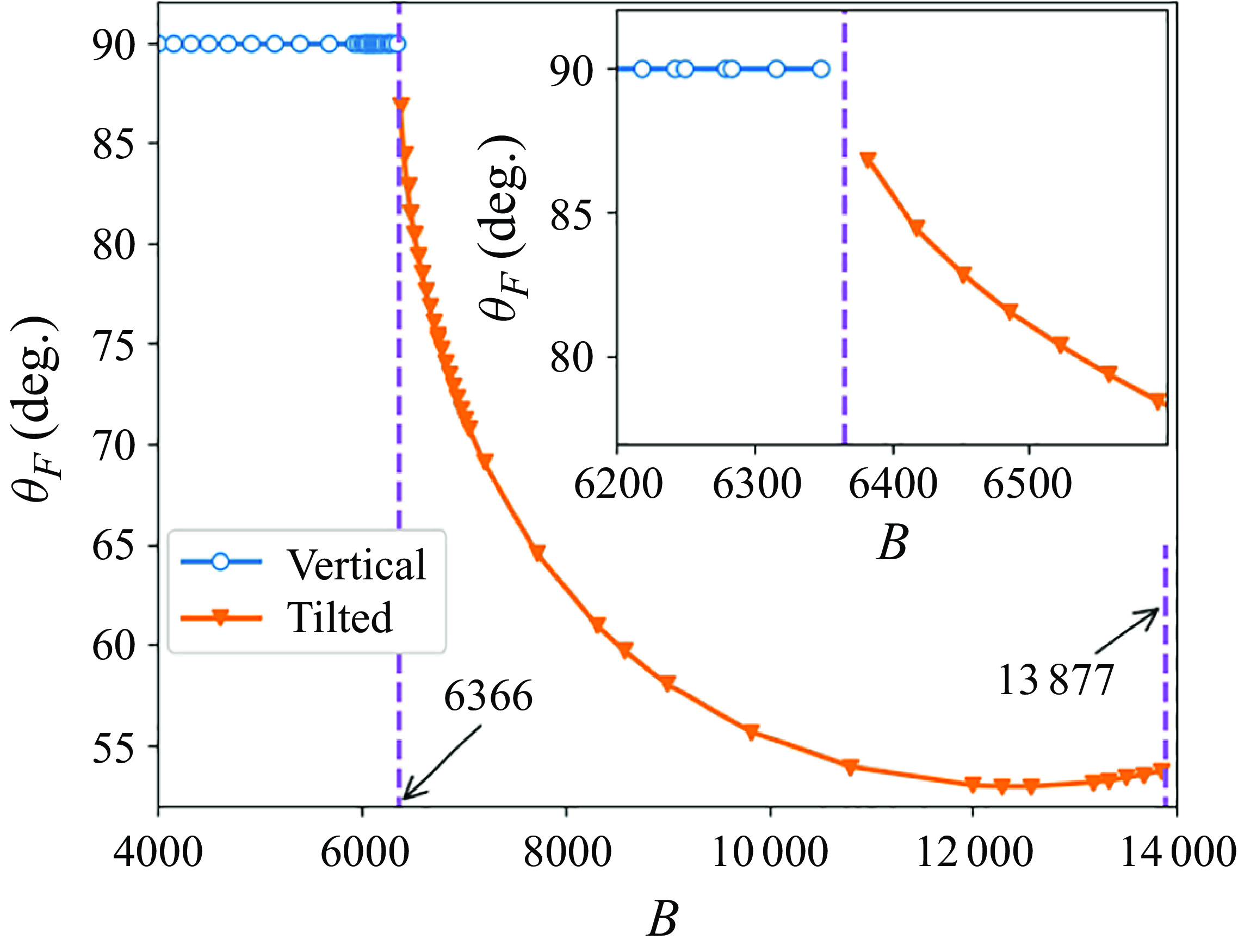
Figure 3. The final polar angle $\theta _{F}$
as a function of the elasto-gravitation number
$\theta _{F}$
as a function of the elasto-gravitation number $B$
for the tilted and vertical modes. Symbols correspond to the numerical data and are connected by solid lines to guide the eye.
$B$
for the tilted and vertical modes. Symbols correspond to the numerical data and are connected by solid lines to guide the eye.
The transition value $B_{crit}$
between the vertical and tilted modes, marked in figure 3, has been determined by analysing how these modes are reached from the initially inclined circular configuration. When the loop tends to the vertical or tilted mode of the characteristic inclination
$B_{crit}$
between the vertical and tilted modes, marked in figure 3, has been determined by analysing how these modes are reached from the initially inclined circular configuration. When the loop tends to the vertical or tilted mode of the characteristic inclination $\theta _F$
from the initial inclination
$\theta _F$
from the initial inclination $\tilde {\theta }_{0} = \theta (t=0)$
at the start of the simulation, the inclination angle
$\tilde {\theta }_{0} = \theta (t=0)$
at the start of the simulation, the inclination angle $\theta$
changes monotonically with time, and the exponential law can fit this relation, as shown in figure 4(a),
$\theta$
changes monotonically with time, and the exponential law can fit this relation, as shown in figure 4(a),
 \begin{equation} \theta (t) = \theta _{F} + ( \tilde {\theta }_{0} - \theta _{F} ) \cdot e^{-t/t_{char}}, \end{equation}
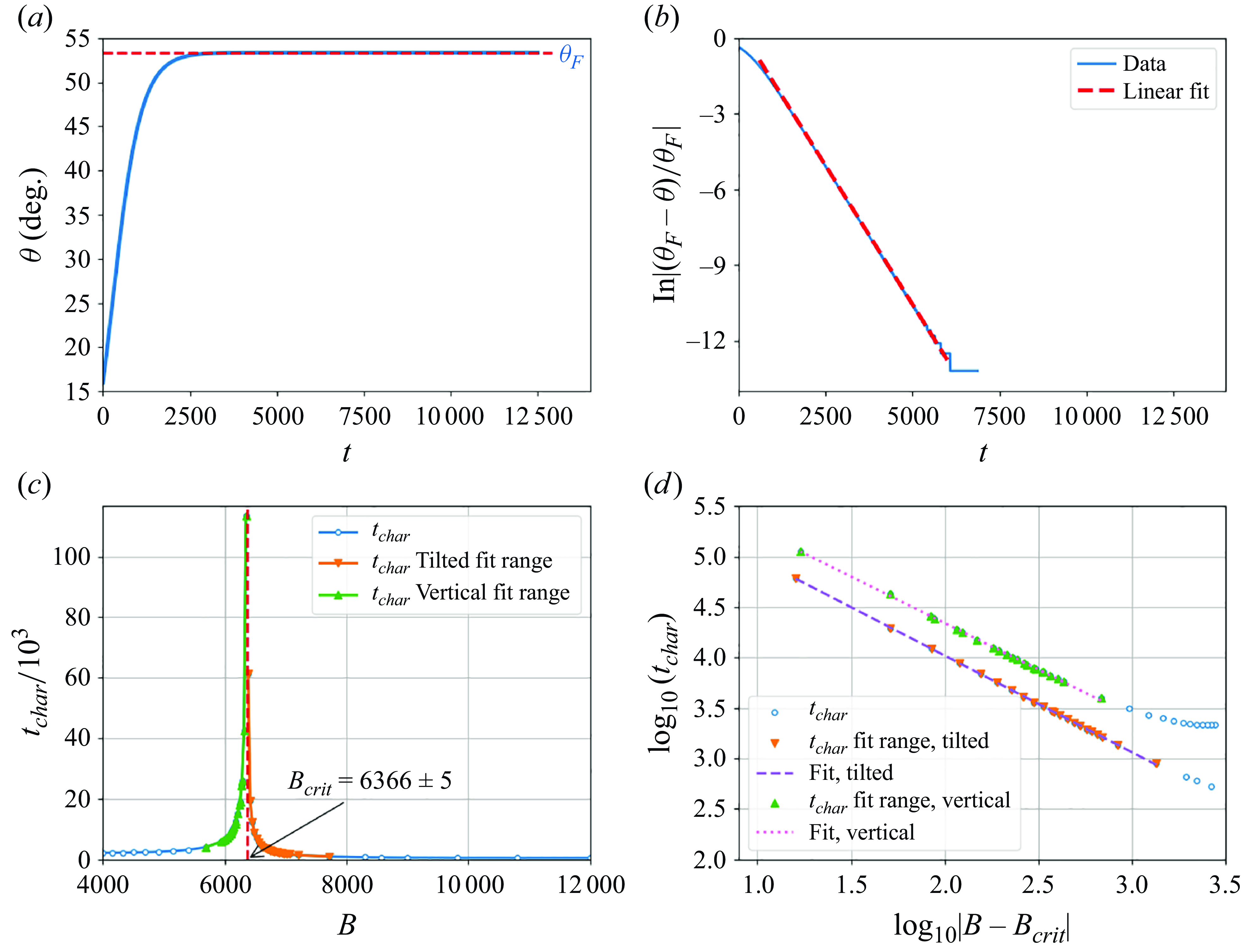
Figure 4. The exponential approach of the polar angle $\theta (t)$
to the final angle
$\theta (t)$
to the final angle $\theta _{F}$
for vertical and tilted modes with different values of
$\theta _{F}$
for vertical and tilted modes with different values of $B$
can be used to estimate
$B$
can be used to estimate $B_{crit}$
between both modes. Here (a)
$B_{crit}$
between both modes. Here (a) $\theta (t)$
for
$\theta (t)$
for $B=13\,501$
with
$B=13\,501$
with $\theta _{F}=53.37^\circ$
; (b)
$\theta _{F}=53.37^\circ$
; (b) $\mathrm{ln} | (\theta _{F} - \theta )/ \theta _{F} |$
is well approximated by the fit (3.1) with
$\mathrm{ln} | (\theta _{F} - \theta )/ \theta _{F} |$
is well approximated by the fit (3.1) with $t_{char}=453$
. (c) The characteristic time
$t_{char}=453$
. (c) The characteristic time $t_{char}$
of the fit (3.1) as a function of the elasto-gravitation number
$t_{char}$
of the fit (3.1) as a function of the elasto-gravitation number $B$
. (d) Log–log plot confirms a power law dependence of
$B$
. (d) Log–log plot confirms a power law dependence of $t_{char}$
on
$t_{char}$
on $|B-B_{crit}|$
near the critical value
$|B-B_{crit}|$
near the critical value $B_{crit}$
.
$B_{crit}$
.
with characteristic time $t_{char}\gt 0$
depending on the elasto-gravitation number
$t_{char}\gt 0$
depending on the elasto-gravitation number $B$
and different for the vertical and tilted modes. Numerical simulations show that when
$B$
and different for the vertical and tilted modes. Numerical simulations show that when $B$
is approaching
$B$
is approaching $B_{crit}$
from either side, the characteristic time
$B_{crit}$
from either side, the characteristic time $t_{char}$
approaches infinity, as presented in figure 4(c). Therefore, the power-law increase is expected,
$t_{char}$
approaches infinity, as presented in figure 4(c). Therefore, the power-law increase is expected,
 \begin{equation} t_{char} = t_{0} \cdot |B-B_{crit}|^{-p}. \end{equation}
In figure 4(d), the fit (3.2) is plotted together with the numerical data. The fitted parameters are $B_{crit} = 6366$
,
$B_{crit} = 6366$
, $(t_0,p)=(1.53 \times 10^6, 0.92)$
for the vertical mode and
$(t_0,p)=(1.53 \times 10^6, 0.92)$
for the vertical mode and $(t_0,p)=(0.86 \times 10^6, 0.96)$
for the tilted mode.
$(t_0,p)=(0.86 \times 10^6, 0.96)$
for the tilted mode.
The fitting procedure in the power law (3.2) involves two coefficients, $B_{crit}$
and
$B_{crit}$
and $p$
, and requires very long simulations to get a reasonable precision. A similar fitting was performed by Ekiel-Jeżewska (Reference Ekiel-Jeżewska2014) for a period of oscillations of a group of particles dependent as a power law on a parameter of the initial configuration,
$p$
, and requires very long simulations to get a reasonable precision. A similar fitting was performed by Ekiel-Jeżewska (Reference Ekiel-Jeżewska2014) for a period of oscillations of a group of particles dependent as a power law on a parameter of the initial configuration, $c-c_{crit}$
. In that case, it was possible to determine the exponent analytically, using an approximation for the relative trajectories.
$c-c_{crit}$
. In that case, it was possible to determine the exponent analytically, using an approximation for the relative trajectories.
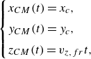
The evolution of the loop’s centre of mass in the vertical and tilted modes can be expressed in the following simple form:
 \begin{equation} \begin{cases} x_{CM}(t)=x_{c} + v_{CM,x} t, \\[4pt] y_{CM}(t)=y_{c}, \\[4pt] z_{CM}(t)=-v_{CM,z} t, \end{cases} \end{equation}
where $x_{c}$
,
$x_{c}$
, $y_{c}$
,
$y_{c}$
, $v_{CM,x} \geqslant 0$
and
$v_{CM,x} \geqslant 0$
and $v_{CM,z}\geqslant 0$
are constants, and in the case of vertical mode,
$v_{CM,z}\geqslant 0$
are constants, and in the case of vertical mode, $v_{CM,x}=0$
. The sedimentation speed
$v_{CM,x}=0$
. The sedimentation speed $v_{CM,z}$
in the vertical mode is almost independent of
$v_{CM,z}$
in the vertical mode is almost independent of $B$
:
$B$
: $1.631 \lesssim v_{CM,z} \lesssim 1.635$
. On the other hand, the velocity
$1.631 \lesssim v_{CM,z} \lesssim 1.635$
. On the other hand, the velocity $v_{CM,x}$
increases and
$v_{CM,x}$
increases and $v_{CM,z}$
decreases with the increase of
$v_{CM,z}$
decreases with the increase of $B\le 12\,000$
, what is caused by the decrease of the inclination angle
$B\le 12\,000$
, what is caused by the decrease of the inclination angle $\theta$
, shown in figure 3, as will be discussed in § 6.
$\theta$
, shown in figure 3, as will be discussed in § 6.
3.3. The rocking and gyrating-rocking-tank-treading modes
In our numerical simulations, elastic loops with the elasto-gravitation number $13\,882 \leqslant B \leqslant 14\,211$
end up in the rocking mode, illustrated in Movie 2 of the Supplementary movies. For slightly larger values,
$13\,882 \leqslant B \leqslant 14\,211$
end up in the rocking mode, illustrated in Movie 2 of the Supplementary movies. For slightly larger values, $14\,248 \leqslant B \leqslant 17\,422$
, a gyrating-rocking-tank-treading mode is reached, as shown in Movie 4 of the Supplementary movies. The common feature of these modes is the existence of periodic in-time oscillations of both orientation angles
$14\,248 \leqslant B \leqslant 17\,422$
, a gyrating-rocking-tank-treading mode is reached, as shown in Movie 4 of the Supplementary movies. The common feature of these modes is the existence of periodic in-time oscillations of both orientation angles $\theta$
and
$\theta$
and $\phi$
, as shown in figure 2(a,c). We first analyse the properties of the rocking mode, and then we describe the gyrating-rocking-tank-treading mode.
$\phi$
, as shown in figure 2(a,c). We first analyse the properties of the rocking mode, and then we describe the gyrating-rocking-tank-treading mode.
When the elasto-gravitation number $B$
increases above the values typical for the tilted mode, the loop ends in a rocking mode instead of the tilted one. The appearance of this mode is illustrated in figure 5(a). In the first stage of the evolution, the loop seems to reach the tilted mode with a certain inclination angle
$B$
increases above the values typical for the tilted mode, the loop ends in a rocking mode instead of the tilted one. The appearance of this mode is illustrated in figure 5(a). In the first stage of the evolution, the loop seems to reach the tilted mode with a certain inclination angle $\theta _{t}$
. However, after a relatively long time, the inclination angle
$\theta _{t}$
. However, after a relatively long time, the inclination angle $\theta (t)$
decreases, and starts oscillating around a lower value
$\theta (t)$
decreases, and starts oscillating around a lower value $\theta _0$
. The periodic oscillations of the angle
$\theta _0$
. The periodic oscillations of the angle $\theta$
, with a constant amplitude
$\theta$
, with a constant amplitude $\theta _2$
and the average
$\theta _2$
and the average $\theta _0\ne 90^\circ$
, are typical for the rocking mode.
$\theta _0\ne 90^\circ$
, are typical for the rocking mode.
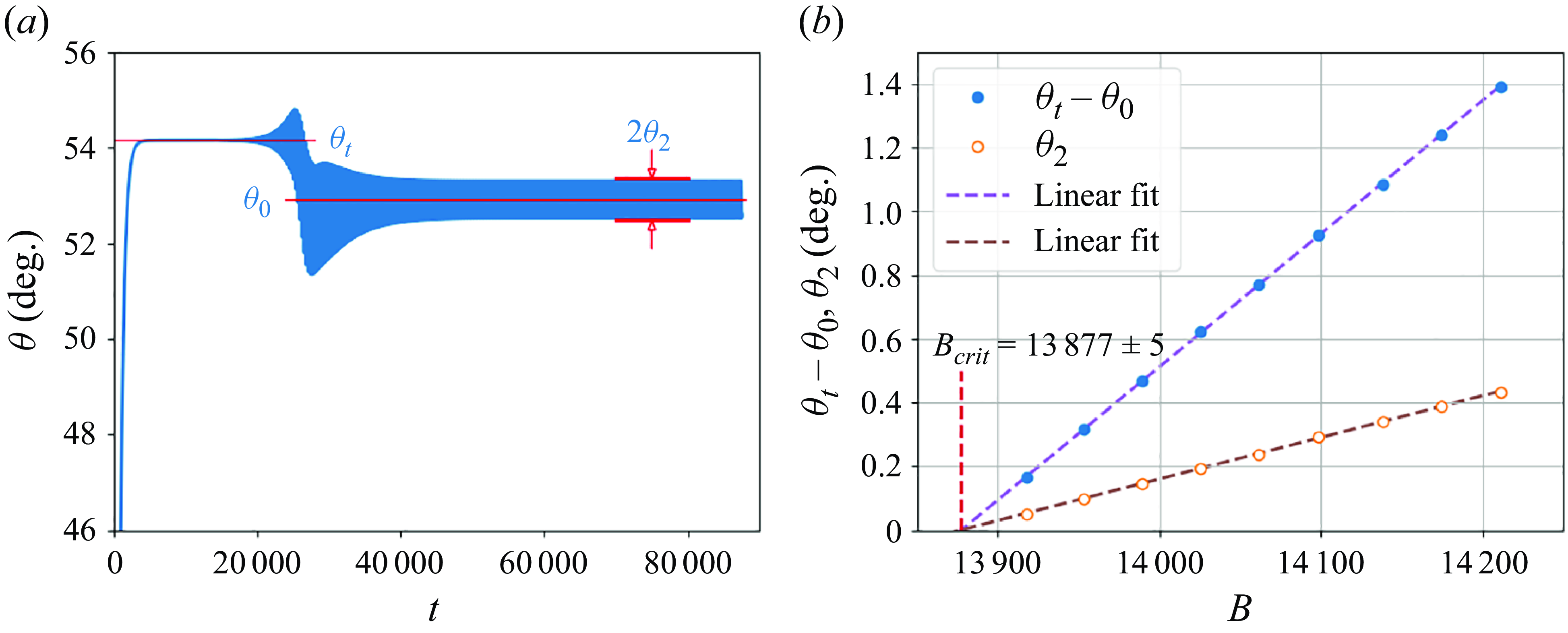
Figure 5. The evolution of $\theta$
for different values of
$\theta$
for different values of $B$
is used to determine
$B$
is used to determine $B_{crit}$
for the transition between tilted and rocking modes. Here (a)
$B_{crit}$
for the transition between tilted and rocking modes. Here (a) $\theta (t)$
for
$\theta (t)$
for $B=14\,174$
. For
$B=14\,174$
. For $4000 \lesssim t \lesssim 18\,000$
, the loop seems to be in the tilted mode with
$4000 \lesssim t \lesssim 18\,000$
, the loop seems to be in the tilted mode with $\theta _{t} \approx 54.16^\circ$
. But later, it destabilises. The periodic rocking motion is observed after the transition phase is finished at
$\theta _{t} \approx 54.16^\circ$
. But later, it destabilises. The periodic rocking motion is observed after the transition phase is finished at $t \approx 55\,000$
. (b) Here
$t \approx 55\,000$
. (b) Here $\theta _t-\theta _0$
and
$\theta _t-\theta _0$
and $\theta _2$
are well-fitted by linear functions of
$\theta _2$
are well-fitted by linear functions of $B$
; they vanish at approximately the same value of
$B$
; they vanish at approximately the same value of $B_{crit} = 13\,877$
, estimated as the transition between tilted and rocking modes.
$B_{crit} = 13\,877$
, estimated as the transition between tilted and rocking modes.
The amplitude $\theta _{2}$
of the rocking oscillations and the difference
$\theta _{2}$
of the rocking oscillations and the difference $\theta _t-\theta _0$
increase linearly with an increase of the elasto-gravitation number
$\theta _t-\theta _0$
increase linearly with an increase of the elasto-gravitation number $B$
as seen in figure 5(b). Linear fits to the simulation data predict that
$B$
as seen in figure 5(b). Linear fits to the simulation data predict that $\theta _{2}$
and
$\theta _{2}$
and $\theta _t-\theta _0$
vanish at approximately the same value
$\theta _t-\theta _0$
vanish at approximately the same value $B=B_{crit} \approx 13\,877$
. This observation indicates that the rocking mode ceases to exist when
$B=B_{crit} \approx 13\,877$
. This observation indicates that the rocking mode ceases to exist when $B$
decreases to
$B$
decreases to $B_{crit}$
.
$B_{crit}$
.
In the rocking mode, the period $T_r={2\pi }/{\omega _r}$
of the azimuthal angle oscillations is twice as large as the period of the polar angle oscillations, as visible in figure 2. For the rocking mode, the period
$T_r={2\pi }/{\omega _r}$
of the azimuthal angle oscillations is twice as large as the period of the polar angle oscillations, as visible in figure 2. For the rocking mode, the period $T_{r}$
decreases gradually with an increase of
$T_{r}$
decreases gradually with an increase of $B$
, as shown in figure 6 (blue triangles). The oscillations of
$B$
, as shown in figure 6 (blue triangles). The oscillations of $\theta$
are around the averaged inclination angle
$\theta$
are around the averaged inclination angle $\theta _0\ne 90^\circ$
. We choose such a reference frame that the oscillations of
$\theta _0\ne 90^\circ$
. We choose such a reference frame that the oscillations of $\phi$
are around the average value equal to zero. The time dependence of
$\phi$
are around the average value equal to zero. The time dependence of $\theta$
and
$\theta$
and $\phi$
can be approximated as
$\phi$
can be approximated as
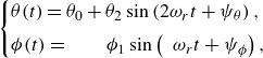 \begin{equation} \begin{cases} \theta (t) = \theta _{0} + \theta _{2} \sin \left ( 2 \omega _{r} t + \psi _{\theta } \right ), \\[4pt] \phi (t) = \mkern 35mu \phi _{1} \sin \left ( \mkern 9mu \omega _{r} t + \psi _{\phi } \right ), \end{cases} \end{equation}
where $\psi _{\theta }$
and
$\psi _{\theta }$
and $\psi _{\phi }$
are the phase shifts, and the amplitudes
$\psi _{\phi }$
are the phase shifts, and the amplitudes $\theta _{2}$
and
$\theta _{2}$
and $\phi _{1}$
dependent on
$\phi _{1}$
dependent on $B$
. The approximation from (3.4) is shown to fit well the numerical data, as demonstrated in Appendix A for an exemplary value of
$B$
. The approximation from (3.4) is shown to fit well the numerical data, as demonstrated in Appendix A for an exemplary value of $B$
. The amplitudes
$B$
. The amplitudes $\theta _{2}$
and
$\theta _{2}$
and $\phi _{1}$
are small. The largest value of
$\phi _{1}$
are small. The largest value of $\phi _1$
, i.e.
$\phi _1$
, i.e. $\phi _{1}=8.52^\circ$
is attained for
$\phi _{1}=8.52^\circ$
is attained for $B=14\,211$
.
$B=14\,211$
.
In contrast, $\theta _0$
is relatively large, as shown in figure 5(a). The averaged inclination of the loop is associated with an averaged horizontal drift of its centre of mass along the
$\theta _0$
is relatively large, as shown in figure 5(a). The averaged inclination of the loop is associated with an averaged horizontal drift of its centre of mass along the $x$
-axis, as illustrated in figure 2(c).
$x$
-axis, as illustrated in figure 2(c).

Figure 6. Dependence of the period $T_r$
of the oscillations on elasto-gravitation number
$T_r$
of the oscillations on elasto-gravitation number $B$
in the rocking mode and in the gyrating-rocking-tank-treading mode.
$B$
in the rocking mode and in the gyrating-rocking-tank-treading mode.
The motion of the loop’s centre of mass in the rocking mode is a superposition of translation with a constant velocity and periodic oscillations. It can be approximated as
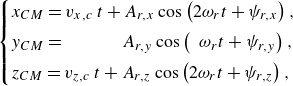 \begin{equation} \begin{cases} x_{CM}=v_{x,c}\, t + A_{r,x} \cos \left ( 2 \omega _{r} t + \psi _{r,x} \right ), \\[4pt] y_{CM}= \mkern 57mu A_{r,y} \cos \left ( \mkern 9mu \omega _{r} t + \psi _{r,y} \right ), \\[4pt] z_{CM}=v_{z,c}\, t + A_{r,z} \cos \left ( 2 \omega _{r} t + \psi _{r,z} \right ), \end{cases} \end{equation}
where $\psi _{r,x}$
,
$\psi _{r,x}$
, $\psi _{r,y}$
and
$\psi _{r,y}$
and $\psi _{r,z}$
are the phase shifts, velocities
$\psi _{r,z}$
are the phase shifts, velocities $v_{x,c}$
and
$v_{x,c}$
and $v_{z,c}$
depend on
$v_{z,c}$
depend on $B$
, and amplitudes
$B$
, and amplitudes $A_{r,x}$
,
$A_{r,x}$
, $A_{r,y}$
and
$A_{r,y}$
and $A_{r,z}$
decrease with a decrease of
$A_{r,z}$
decrease with a decrease of $B$
. The velocities
$B$
. The velocities $v_{x,c}$
and
$v_{x,c}$
and $v_{z,c} = -v_{CM,z}$
depend on
$v_{z,c} = -v_{CM,z}$
depend on $B$
very weakly, as shown in figures 7 and 17(a). The approximation from (3.5) is shown to fit well the numerical data, as demonstrated in Appendix A for an exemplary value of
$B$
very weakly, as shown in figures 7 and 17(a). The approximation from (3.5) is shown to fit well the numerical data, as demonstrated in Appendix A for an exemplary value of $B$
.
$B$
.
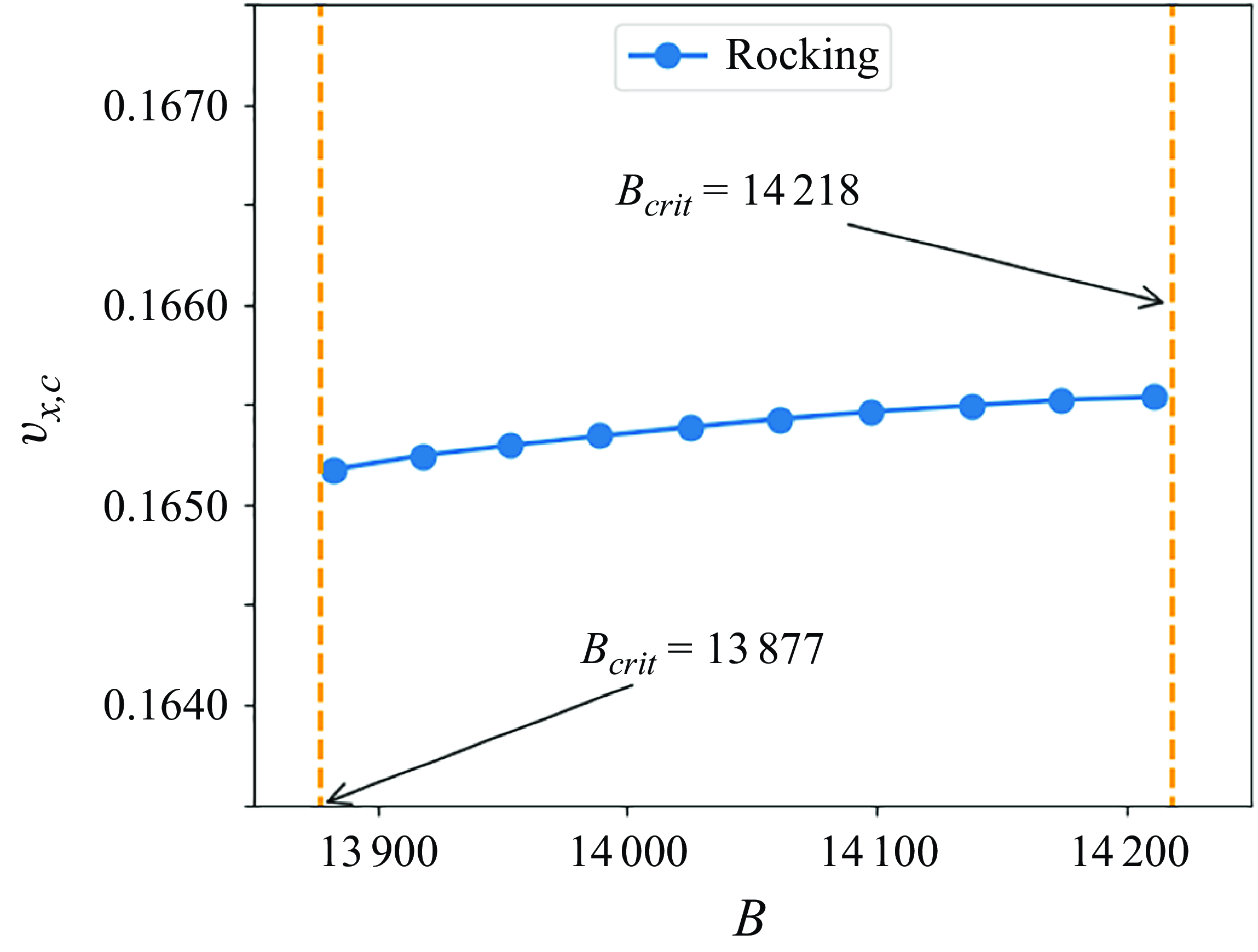
Figure 7. The mean $x$
-component
$x$
-component $v_{x,c}$
of the horizontal velocity of the elastic loop in the rocking mode as a function of elasto-gravitation number
$v_{x,c}$
of the horizontal velocity of the elastic loop in the rocking mode as a function of elasto-gravitation number $B$
. Here
$B$
. Here $v_{y,c}=0$
, see (3.5).
$v_{y,c}=0$
, see (3.5).
The gyrating-rocking-tank-treading (GRTT) mode is observed for moderately elastic loops with elasto-gravitation number $B$
in the range
$B$
in the range $14\,248 \leqslant B \leqslant 17\,422$
. As a part of this name indicates, the loop ‘gyrates’ – it rotates with a constant angular velocity
$14\,248 \leqslant B \leqslant 17\,422$
. As a part of this name indicates, the loop ‘gyrates’ – it rotates with a constant angular velocity $\omega _g$
around a vertical axis, and also performs ‘rocking’ oscillations with the frequency
$\omega _g$
around a vertical axis, and also performs ‘rocking’ oscillations with the frequency $\omega _r$
, similar to in the rocking mode. The polar angle is a periodic function of time, with the period
$\omega _r$
, similar to in the rocking mode. The polar angle is a periodic function of time, with the period $T_r=2\pi /\omega _r$
. The azimuthal angle is a superposition of the linear growth in time at the rate equal to
$T_r=2\pi /\omega _r$
. The azimuthal angle is a superposition of the linear growth in time at the rate equal to $\omega _g$
and a periodic function with the period
$\omega _g$
and a periodic function with the period $T_r$
. The time-dependent angles
$T_r$
. The time-dependent angles $\theta (t)$
and
$\theta (t)$
and $\phi (t)$
can be approximated as
$\phi (t)$
can be approximated as
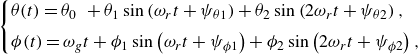 \begin{equation} \begin{cases} \theta (t) = \theta _{0} \; \; + \theta _{1} \sin \left ( \omega _{r} t + \psi _{\theta 1} \right ) + \theta _{2} \sin \left ( 2 \omega _{r} t + \psi _{\theta 2} \right ), \\[4pt] \phi (t) = \omega _g t + \phi _{1} \sin \left ( \omega _{r} t + \psi _{\phi 1} \right ) + \phi _{2} \sin \left ( 2 \omega _{r} t + \psi _{\phi 2} \right ), \end{cases} \end{equation}
where the parameters depend on elasto-gravitation number $B$
. In general, two frequencies are needed in (3.6).
$B$
. In general, two frequencies are needed in (3.6).
The evolution of the loop’s centre of mass as a function of time is more complex. The horizontal projection of the centre-of-mass trajectory, shown in figure 2(b), involves two characteristic frequencies, $\omega _g$
and
$\omega _g$
and $\omega _r$
, with in general irrational ratio. Therefore, the centre-of-mass motion, in general, is quasiperiodic. It can be approximated by the following equations:
$\omega _r$
, with in general irrational ratio. Therefore, the centre-of-mass motion, in general, is quasiperiodic. It can be approximated by the following equations:
 \begin{equation} \hspace {-3.5pt} \begin{cases} \! x_{CM} {=} x_{c} + A_{g} \cos \left ( \omega _{g} t \right ) + A_{r,xy} [ \cos ( ( \omega _{r} - \omega _{g} ) t + \phi _{r,xy_{1}} ) + \cos ( ( \omega _{r} + \omega _{g} ) t + \phi _{r,xy_{2}} ) ], \\[6pt] \! y_{CM} {=} y_{c} + A_{g} \sin ( \omega _{g} t ) + A_{r,xy} [ \sin ( ( \omega _{r} - \omega _{g} ) t + \phi _{r,xy_{1}} ) + \sin ( ( \omega _{r} + \omega _{g} ) t + \phi _{r,xy_{2}} ) ], \\[6pt] \! z_{CM} {=} v_{z,c} t + A_{r,z} \sin ( \omega _{r} t + \phi _{r,z} ), \end{cases} \end{equation}
with the parameters dependent on $B$
. Here
$B$
. Here $A_{g}$
is the amplitude (the averaged radius) of the gyrating motion and the amplitudes
$A_{g}$
is the amplitude (the averaged radius) of the gyrating motion and the amplitudes $A_{r,xy}$
and
$A_{r,xy}$
and $A_{r,z}$
are associated with the oscillating ‘rocking’ motion. The constants
$A_{r,z}$
are associated with the oscillating ‘rocking’ motion. The constants $x_{c}$
and
$x_{c}$
and $y_{c}$
are somewhat arbitrary. Their values are set at the end of a transition phase. The sedimentation velocity
$y_{c}$
are somewhat arbitrary. Their values are set at the end of a transition phase. The sedimentation velocity $v_{z,c}$
is constant in time. The approximations from (3.6)–(3.7) are shown to fit the numerical data well, as demonstrated in Appendix A for an exemplary value of
$v_{z,c}$
is constant in time. The approximations from (3.6)–(3.7) are shown to fit the numerical data well, as demonstrated in Appendix A for an exemplary value of $B$
.
$B$
.
The function $T_r(B)$
is shown in figure 6. The period of the oscillations in the GRTT mode smoothly extends
$T_r(B)$
is shown in figure 6. The period of the oscillations in the GRTT mode smoothly extends $T_r(B)$
from the rocking mode for larger values of
$T_r(B)$
from the rocking mode for larger values of $B$
. The characteristic time scale of gyration,
$B$
. The characteristic time scale of gyration, $T_g=2\pi /\omega _g$
, is plotted as a function of
$T_g=2\pi /\omega _g$
, is plotted as a function of $B$
in figure 8(a). It is clear that
$B$
in figure 8(a). It is clear that $T_g$
increases significantly with the decrease of
$T_g$
increases significantly with the decrease of $B$
. We expect that
$B$
. We expect that $T_g$
might diverge at a critical value of
$T_g$
might diverge at a critical value of $B_{crit}$
as
$B_{crit}$
as
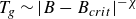 \begin{equation} T_g \sim |B-B_{crit}|^{-\chi } \end{equation}
that allowed us to identify $B_{crit} = 14\,218$
as the critical value of
$B_{crit} = 14\,218$
as the critical value of $B$
corresponding to the transition between the rocking and GRTT modes (see Appendix B for details).
$B$
corresponding to the transition between the rocking and GRTT modes (see Appendix B for details).
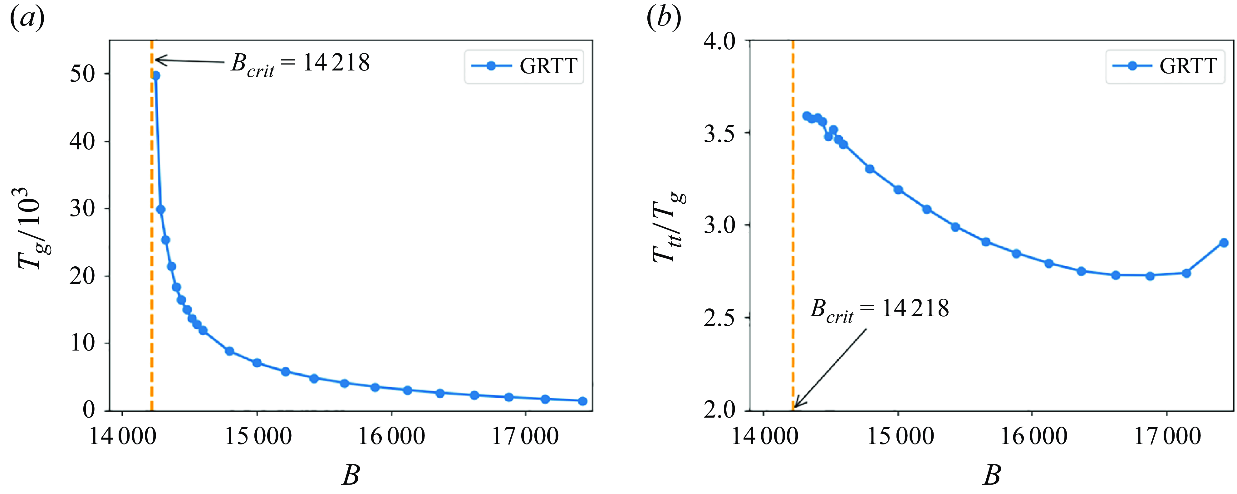
Figure 8. Dependence of the characteristic time scales of the GRTT motion on the elasto-gravitation number $B$
: (a)
$B$
: (a) $T_g$
; (b)
$T_g$
; (b) $T_{tt}/T_g$
.
$T_{tt}/T_g$
.
The increase of $T_g$
is related to the increase of the amplitude (the averaged radius)
$T_g$
is related to the increase of the amplitude (the averaged radius) $A_{g}$
of the gyrating motion. Here
$A_{g}$
of the gyrating motion. Here $T_g$
is proportional to
$T_g$
is proportional to $A_{g}$
, with the approximately constant gyration velocity,
$A_{g}$
, with the approximately constant gyration velocity, $ v_g=A_g\,\omega _g \approx 0.16$
, as shown in figure 9.
$ v_g=A_g\,\omega _g \approx 0.16$
, as shown in figure 9.
Figure 9. In the GRTT mode, the averaged radius $A_r$
of the horizontal projection of the centre-of-mass trajectories increases with the decrease of
$A_r$
of the horizontal projection of the centre-of-mass trajectories increases with the decrease of $B$
, as shown in (a), while the gyration velocity is almost constant, as visible in (b).
$B$
, as shown in (a), while the gyration velocity is almost constant, as visible in (b).
So far, we have analysed only global features of the loop, such as the polar and azimuthal angles and the centre-of-mass coordinates or velocities. Some information on the loop shape can be provided by the time-dependent local curvature at each specific bead $i$
, which is calculated as the inverse of the radius of a circle circumscribed on the centres of three consecutive beads
$i$
, which is calculated as the inverse of the radius of a circle circumscribed on the centres of three consecutive beads $i-1,i,i+1$
(Słowicka et al. Reference Słowicka, Xue, Sznajder, Nunes, Stone and Ekiel-Jeżewska2022). An example of the time-dependent curvature at two beads for
$i-1,i,i+1$
(Słowicka et al. Reference Słowicka, Xue, Sznajder, Nunes, Stone and Ekiel-Jeżewska2022). An example of the time-dependent curvature at two beads for $B=15\,000$
is shown in figure 10. The local curvature has approximately the same envelope function of time for both beads but with a time shift. The shift corresponds to the tank-treading-like motion of each bead along the loop shape. This motion may be described as the beads undergoing a periodic alteration in their spatial position with respect to the centre of mass. It bears a resemblance to the tank-treading motion in which the beads move along the fixed shape (see § 3.5). Note that the overall shape of the loop in the GRTT mode is not fixed; the rocking oscillations take place.
$B=15\,000$
is shown in figure 10. The local curvature has approximately the same envelope function of time for both beads but with a time shift. The shift corresponds to the tank-treading-like motion of each bead along the loop shape. This motion may be described as the beads undergoing a periodic alteration in their spatial position with respect to the centre of mass. It bears a resemblance to the tank-treading motion in which the beads move along the fixed shape (see § 3.5). Note that the overall shape of the loop in the GRTT mode is not fixed; the rocking oscillations take place.
The period $T_{tt}$
associated with the tank-treading-like motion can be also identified through an analysis of the time dependence of
$T_{tt}$
associated with the tank-treading-like motion can be also identified through an analysis of the time dependence of $z-z_{CM}$
for any given bead. Since beads undergo a periodic alteration in their spatial position with respect to the centre of mass, the quantity
$z-z_{CM}$
for any given bead. Since beads undergo a periodic alteration in their spatial position with respect to the centre of mass, the quantity $z-z_{CM}$
will exhibit maxima and minima with a period of
$z-z_{CM}$
will exhibit maxima and minima with a period of $T_{tt}$
, similar to the local curvature.
$T_{tt}$
, similar to the local curvature.
The time shift between the beads can be utilised to identify the value of $T_{tt}$
also when the time range of the observed GRTT mode is smaller than the period
$T_{tt}$
also when the time range of the observed GRTT mode is smaller than the period $T_{tt}$
, which is particularly relevant in cases with smaller values of
$T_{tt}$
, which is particularly relevant in cases with smaller values of $B$
, specifically when
$B$
, specifically when $B \le 14\,556$
.
$B \le 14\,556$
.
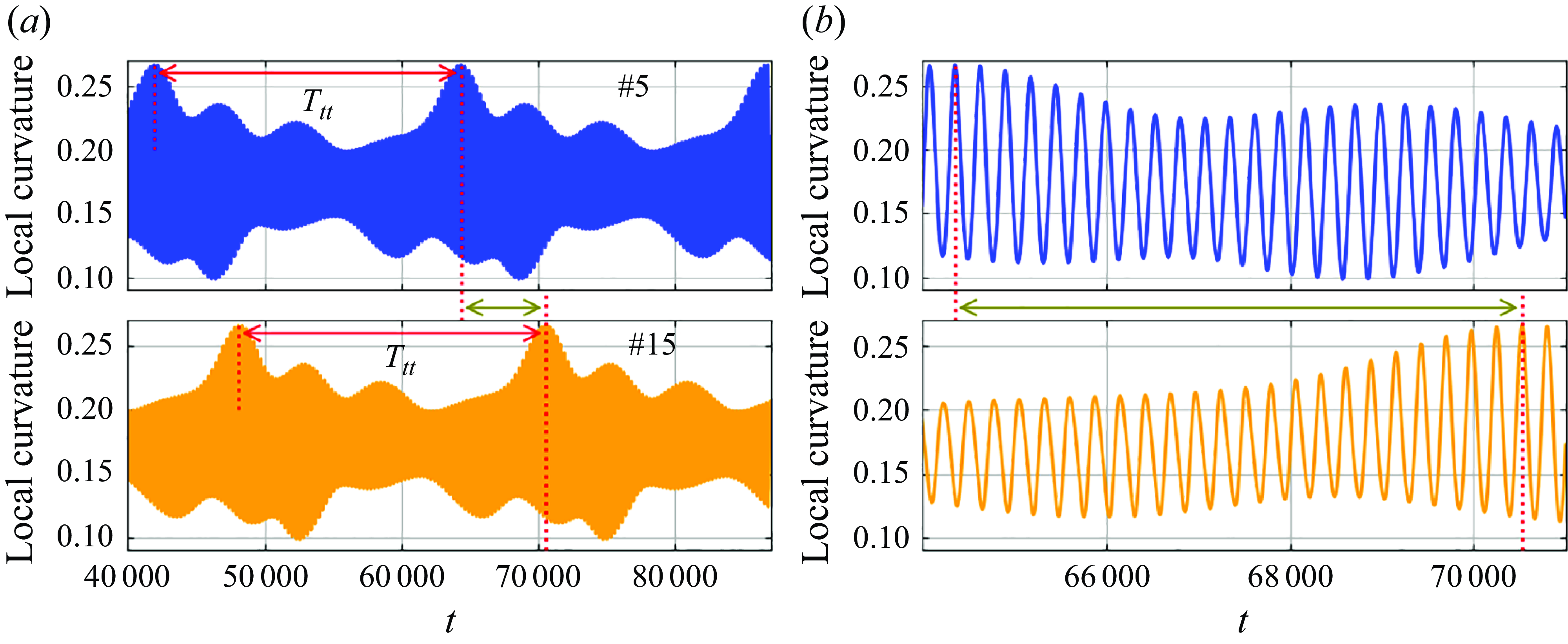
Figure 10. Time dependence of the local curvature for the fifth and $15$
th beads in the GRTT mode with
$15$
th beads in the GRTT mode with $B=15\,000$
is described by approximately the same envelope function of a period
$B=15\,000$
is described by approximately the same envelope function of a period $T_{tt}$
, but shifted in time by
$T_{tt}$
, but shifted in time by $10T_{tt}/36$
, as shown in (a). Oscillations of the local curvature at a short-time scale
$10T_{tt}/36$
, as shown in (a). Oscillations of the local curvature at a short-time scale $T_r$
due to the rocking motion are seen in (b).
$T_r$
due to the rocking motion are seen in (b).
3.4. The frozen rotating mode
The frozen rotating mode is observed for relatively elastic loops with values of the elasto-gravitation number $B$
being in the range of
$B$
being in the range of $17\,477 \leqslant B \leqslant 32\,733$
. In this mode, the loop settles vertically with a constant velocity
$17\,477 \leqslant B \leqslant 32\,733$
. In this mode, the loop settles vertically with a constant velocity $v_{z,fr}$
and spins with a constant angular velocity
$v_{z,fr}$
and spins with a constant angular velocity $\omega _{fr}$
around a vertical axis containing the loop centre of mass. The angles
$\omega _{fr}$
around a vertical axis containing the loop centre of mass. The angles $\theta$
and
$\theta$
and $\phi$
, plotted in figure 2, are
$\phi$
, plotted in figure 2, are
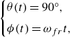 \begin{equation} \begin{cases} \theta (t) = 90^{\circ }, \\[4pt] \phi (t) = \omega _{fr} t, \end{cases} \end{equation}
where the period of rotation $T_{fr}=2\pi /\omega _{fr}$
depends on elasto-gravitation number
$T_{fr}=2\pi /\omega _{fr}$
depends on elasto-gravitation number $B$
as shown in figure 11. The evolution of the loop’s centre of mass is described by the following simple equations:
$B$
as shown in figure 11. The evolution of the loop’s centre of mass is described by the following simple equations:
 \begin{equation} \begin{cases} x_{CM}(t)=x_{c}, \\[4pt] y_{CM}(t)=y_{c}, \\[4pt] z_{CM}(t)=v_{z,fr} t, \end{cases} \end{equation}
where $x_{c}$
,
$x_{c}$
, $y_{c}$
and
$y_{c}$
and $v_{z,fr}$
are constants, and the sedimentation velocity
$v_{z,fr}$
are constants, and the sedimentation velocity $v_{z,fr}$
is almost independent on
$v_{z,fr}$
is almost independent on $B$
,
$B$
, $1.660 \lesssim \lvert v_{z,fr} \rvert \lesssim 1.664$
, as it will be discussed in § 5.
$1.660 \lesssim \lvert v_{z,fr} \rvert \lesssim 1.664$
, as it will be discussed in § 5.
Note that for the selected values of $B$
, namely for
$B$
, namely for $B=18\,622$
,
$B=18\,622$
, $B=18\,945$
,
$B=18\,945$
, $B=19\,286$
and
$B=19\,286$
and $B=19\,634$
, the frozen rotating mode could not be achieved within the monitored simulation time of
$B=19\,634$
, the frozen rotating mode could not be achieved within the monitored simulation time of $88\,000$
. The final stage of the evolution for these values of
$88\,000$
. The final stage of the evolution for these values of $B$
(not shown here) contains features similar to the irregular mode observed for sedimenting highly elastic fibres (Melikhov & Ekiel-Jeżewska Reference Melikhov and Ekiel-Jeżewska2024).
$B$
(not shown here) contains features similar to the irregular mode observed for sedimenting highly elastic fibres (Melikhov & Ekiel-Jeżewska Reference Melikhov and Ekiel-Jeżewska2024).

Figure 11. Dependence of the period $T_{fr}$
of the loop rotation on the elasto-gravitation number
$T_{fr}$
of the loop rotation on the elasto-gravitation number $B$
in the frozen rotating mode reached from a flat inclined circle as the initial configuration. The gap between the dots indicates the range of
$B$
in the frozen rotating mode reached from a flat inclined circle as the initial configuration. The gap between the dots indicates the range of $B$
corresponding to an irregular mode.
$B$
corresponding to an irregular mode.
3.5. The tank-treading, swinging, flapping and irregular modes
In the tank-treading, swinging, flapping and irregular modes, a significant out-of-plane deformation of the loop shape is observed. The tank-treading mode was found for $B=34\,843$
. The mode is characterised by the loop having a fixed shape that rotates about a vertical axis with a period
$B=34\,843$
. The mode is characterised by the loop having a fixed shape that rotates about a vertical axis with a period $T_{rot}=52$
and the constant angular velocity (the azimuthal angle
$T_{rot}=52$
and the constant angular velocity (the azimuthal angle $\phi$
changes linearly with time). The centre of mass moves along a helix of a small horizontal circular cross-section with radius
$\phi$
changes linearly with time). The centre of mass moves along a helix of a small horizontal circular cross-section with radius $r_{rot} \approx 1$
. The polar angle
$r_{rot} \approx 1$
. The polar angle $\theta = 0 ^\circ$
but the shape is far from being planar. In addition, there is also a translation of the beads along the loop with a period
$\theta = 0 ^\circ$
but the shape is far from being planar. In addition, there is also a translation of the beads along the loop with a period $T_{tt}=96$
. The specifics of the structural configuration and the flow of beads are presented in Movies 7 and 8 of the Supplementary movies, confirming that this mode is analogous to the tank-treading mode observed in Gruziel-Słomka et al. (Reference Gruziel-Słomka, Kondratiuk, Szymczak and Ekiel-Jeżewska2019).
$T_{tt}=96$
. The specifics of the structural configuration and the flow of beads are presented in Movies 7 and 8 of the Supplementary movies, confirming that this mode is analogous to the tank-treading mode observed in Gruziel-Słomka et al. (Reference Gruziel-Słomka, Kondratiuk, Szymczak and Ekiel-Jeżewska2019).
The swinging mode, analogous to the swinging mode reported in Gruziel-Słomka et al. (Reference Gruziel-Słomka, Kondratiuk, Szymczak and Ekiel-Jeżewska2019), is observed for two values of the elasto-gravitation number, $B=35\,993$
and
$B=35\,993$
and $37\,244$
, with the periods
$37\,244$
, with the periods $T_{swing}=303$
and
$T_{swing}=303$
and $308$
, respectively. It involves significant time-dependent periodic deformations of the loop shape, as shown in Movie 9 of the Supplementary movies. At each time instant, the shape is symmetric with respect to a vertical plane (
$308$
, respectively. It involves significant time-dependent periodic deformations of the loop shape, as shown in Movie 9 of the Supplementary movies. At each time instant, the shape is symmetric with respect to a vertical plane ( $xz$
plane in Movie 9 of the Supplementary movies). Therefore, the motion of the centre of mass is restricted to this plane. Two cases of the swinging mode exhibit slight differences in the one-dimensional horizontal drift of the centre of mass. For
$xz$
plane in Movie 9 of the Supplementary movies). Therefore, the motion of the centre of mass is restricted to this plane. Two cases of the swinging mode exhibit slight differences in the one-dimensional horizontal drift of the centre of mass. For $B=35\,993$
, the centre of mass of the loop exhibits symmetric oscillations with the amplitude
$B=35\,993$
, the centre of mass of the loop exhibits symmetric oscillations with the amplitude $7d$
about a fixed position, resulting in no horizontal displacement after a single swinging cycle. In contrast, for
$7d$
about a fixed position, resulting in no horizontal displacement after a single swinging cycle. In contrast, for $B=37\,244$
, the forward and backward motions of the centre of mass of the loop are not symmetric, resulting in a horizontal displacement of
$B=37\,244$
, the forward and backward motions of the centre of mass of the loop are not symmetric, resulting in a horizontal displacement of $2 d$
after each swinging cycle.
$2 d$
after each swinging cycle.
The flapping mode is observed for $B=40\,000$
with the period of
$B=40\,000$
with the period of $T_{flap}=157$
. The loop shape undergoes considerable time-dependent periodic deformations, as shown in Movie 10 of the Supplementary movies. The configuration changes from an almost flat and almost horizontal shape to a severely bent 3-D shape. In contrast to the swinging mode, all subsequent configurations possess two vertical planes of symmetry perpendicular to each other. Therefore, the centre of mass does not move horizontally. This mode is also analogous to the flapping mode reported in Gruziel-Słomka et al. (Reference Gruziel-Słomka, Kondratiuk, Szymczak and Ekiel-Jeżewska2019).
$T_{flap}=157$
. The loop shape undergoes considerable time-dependent periodic deformations, as shown in Movie 10 of the Supplementary movies. The configuration changes from an almost flat and almost horizontal shape to a severely bent 3-D shape. In contrast to the swinging mode, all subsequent configurations possess two vertical planes of symmetry perpendicular to each other. Therefore, the centre of mass does not move horizontally. This mode is also analogous to the flapping mode reported in Gruziel-Słomka et al. (Reference Gruziel-Słomka, Kondratiuk, Szymczak and Ekiel-Jeżewska2019).
The irregular mode is observed for $B=33\,746$
, and for several other values of
$B=33\,746$
, and for several other values of $B$
, as discussed in § 3.4. The mode is characterised by irregular rotations and oscillations of the centre of mass trajectory and considerable irregular deformations of the loop shape with time. This mode is analogous to the irregular mode observed in the case of sedimenting fibres reported in Melikhov & Ekiel-Jeżewska (Reference Melikhov and Ekiel-Jeżewska2024).
$B$
, as discussed in § 3.4. The mode is characterised by irregular rotations and oscillations of the centre of mass trajectory and considerable irregular deformations of the loop shape with time. This mode is analogous to the irregular mode observed in the case of sedimenting fibres reported in Melikhov & Ekiel-Jeżewska (Reference Melikhov and Ekiel-Jeżewska2024).
3.6. Diagram of the modes
Different attracting dynamical modes, reached from the initially inclined circular configuration, for different ranges of the elasto-gravitation number $B$
, are shown as a phase diagram in figure 12. The evolution of shapes in these modes is illustrated in the Supplementary movies.
$B$
, are shown as a phase diagram in figure 12. The evolution of shapes in these modes is illustrated in the Supplementary movies.
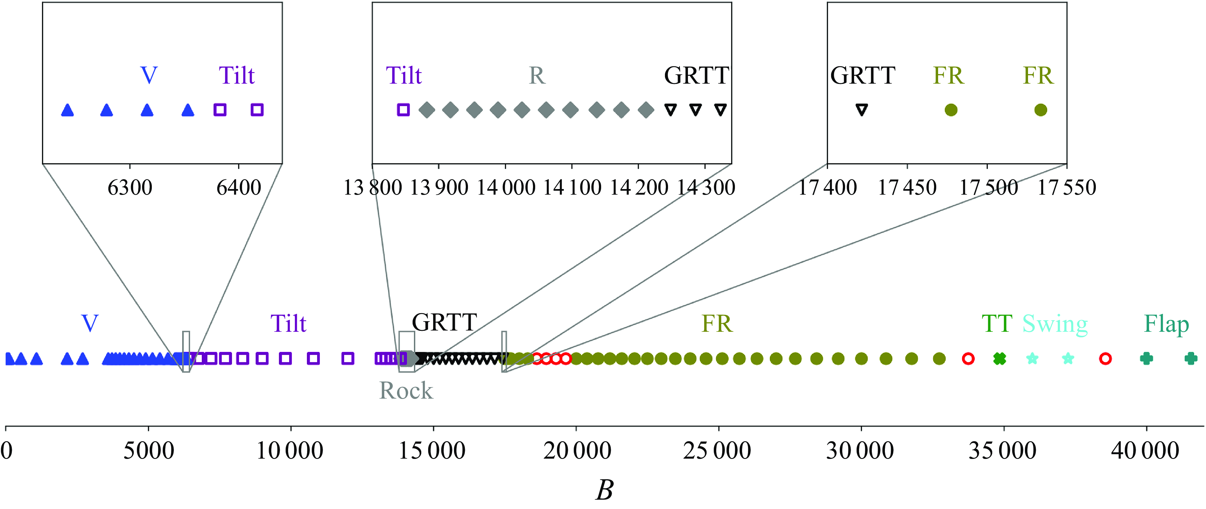
Figure 12. Dependence of attracting dynamical modes on elasto-gravitation number $B$
. Initially, the loop is planar, circular and inclined, typically at
$B$
. Initially, the loop is planar, circular and inclined, typically at $\theta \!=\!16^\circ$
. Critical values of
$\theta \!=\!16^\circ$
. Critical values of $B$
separating distinct modes are
$B$
separating distinct modes are $6366$
(vertical-tilted),
$6366$
(vertical-tilted), $13\,877$
(tilted-rocking) and
$13\,877$
(tilted-rocking) and $14\,218$
(rocking-GRTT). The empty circles correspond to an irregular mode.
$14\,218$
(rocking-GRTT). The empty circles correspond to an irregular mode.
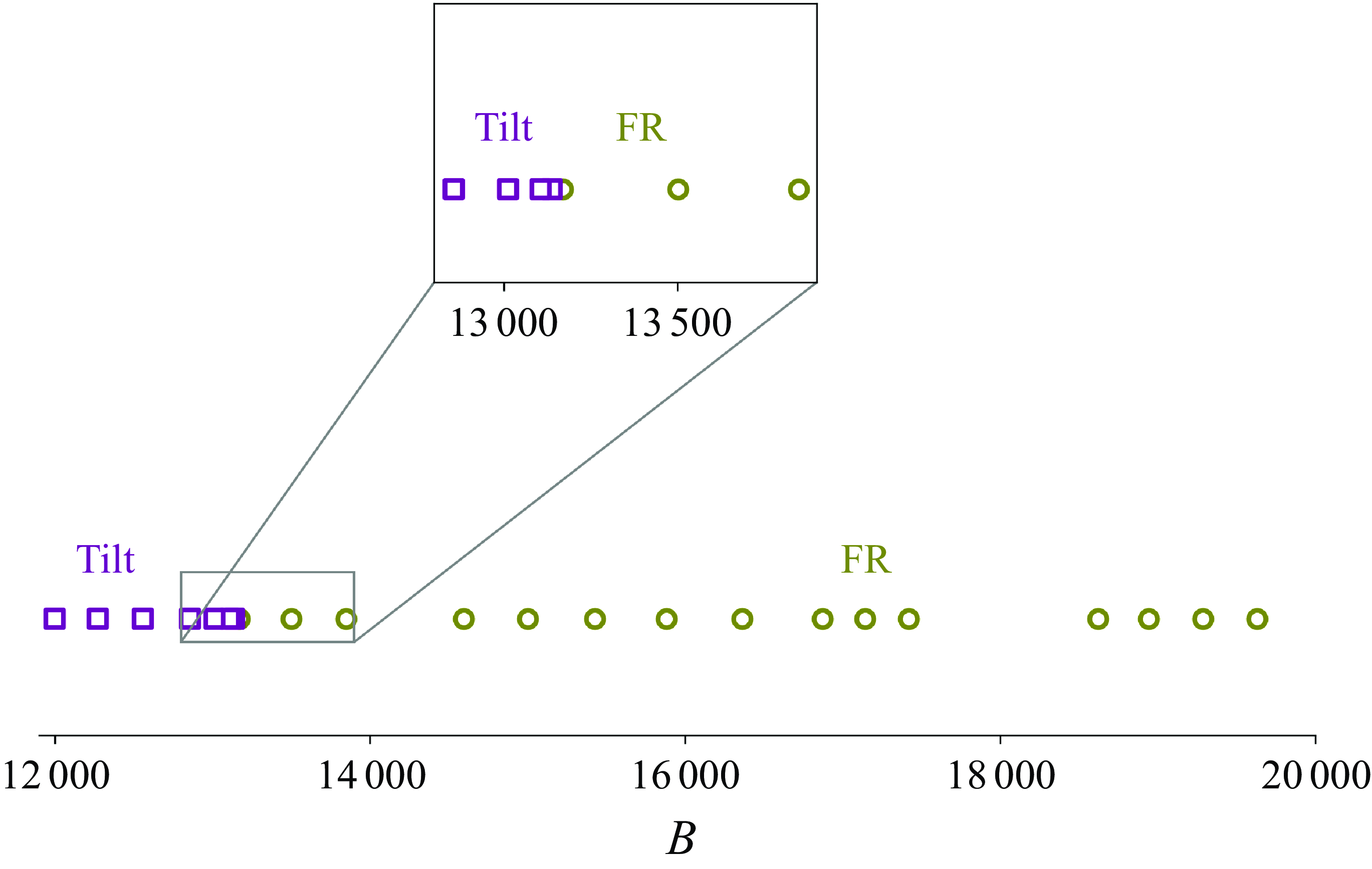
Figure 13. Dependence of attracting dynamical modes on elasto-gravitation number $B$
in the case of the non-planar initial configuration. The critical value of
$B$
in the case of the non-planar initial configuration. The critical value of $B$
separating the tilted and frozen rotating modes is
$B$
separating the tilted and frozen rotating modes is $13\,167$
.
$13\,167$
.
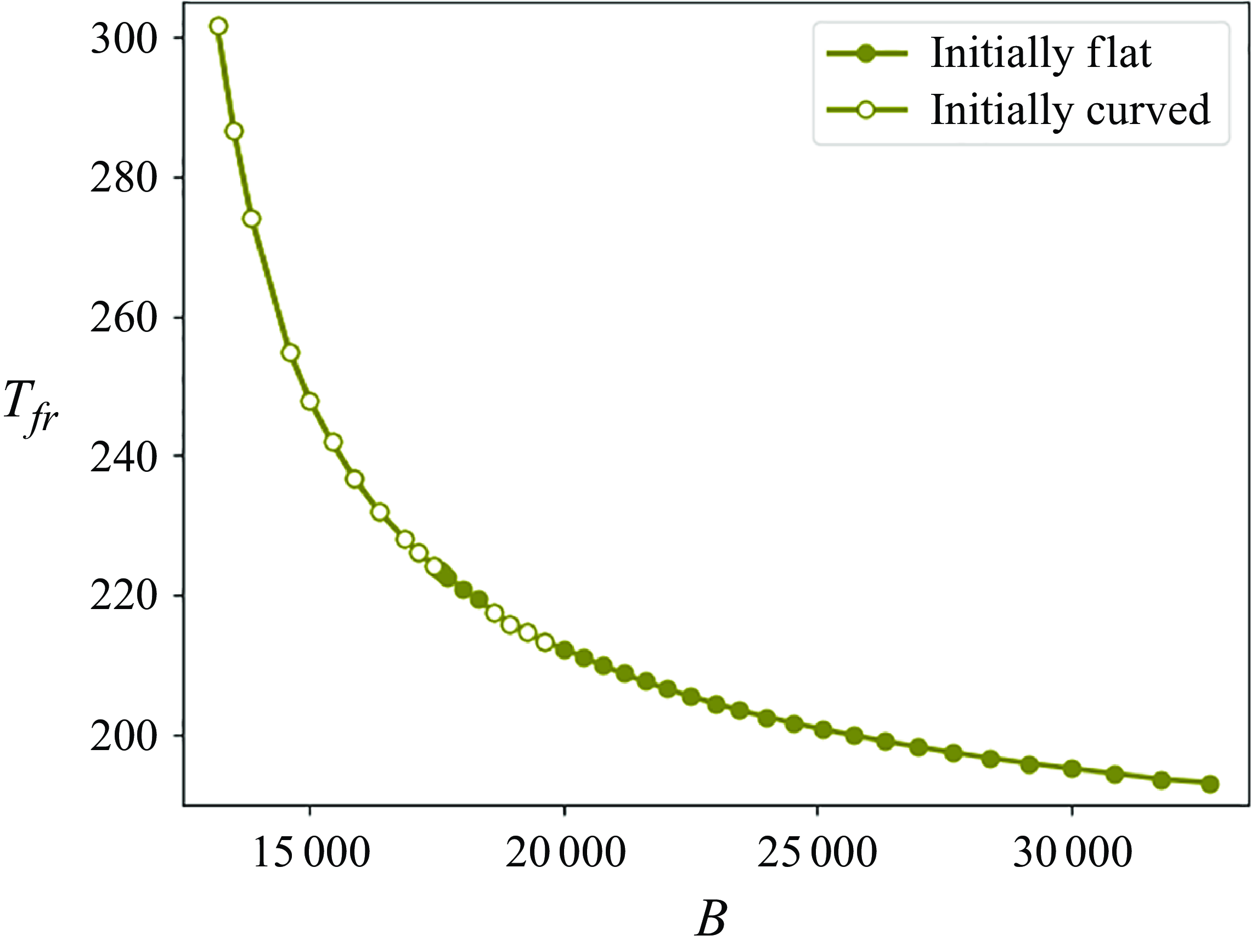
Figure 14. Dependence of the period $T_{fr}$
of the loop rotation on the elasto-gravitation number
$T_{fr}$
of the loop rotation on the elasto-gravitation number $B$
in the frozen rotating mode approached from two different initial conditions: a flat inclined circle, or a non-planar loop, as explained in the text.
$B$
in the frozen rotating mode approached from two different initial conditions: a flat inclined circle, or a non-planar loop, as explained in the text.
4. The frozen rotating mode reached from a non-planar initial configuration
It is known that different attracting dynamical modes can coexist, reached from different initial configurations, as shown in figure 20 in Gruziel-Słomka et al. (2019). Of special interest is the frozen rotating mode, with a fixed shape. Therefore, in this work, we check if the frozen rotating mode can exist for a wider range of $B$
if a different initial configuration is chosen. As a non-planar initial configuration for a chosen value of
$B$
if a different initial configuration is chosen. As a non-planar initial configuration for a chosen value of $B$
, we took the final configuration in the sedimentation of the loop with one of the closest values of
$B$
, we took the final configuration in the sedimentation of the loop with one of the closest values of $B$
that ended up in the frozen rotating mode. We performed numerical simulations for
$B$
that ended up in the frozen rotating mode. We performed numerical simulations for $12\,000 \leqslant B \leqslant 17\,422$
and
$12\,000 \leqslant B \leqslant 17\,422$
and $18\,622 \leqslant B \leqslant 19\,634$
. The last range corresponds to the values of
$18\,622 \leqslant B \leqslant 19\,634$
. The last range corresponds to the values of $B$
that result in irregular modes if a flat inclined circle as the initial configuration was selected. For the non-planar initial configuration, in the same range of
$B$
that result in irregular modes if a flat inclined circle as the initial configuration was selected. For the non-planar initial configuration, in the same range of $B$
, the loop ends up in the frozen rotating mode with a shape slightly different than the initial one.
$B$
, the loop ends up in the frozen rotating mode with a shape slightly different than the initial one.
This behaviour differs from the evolution from a flat inclined initial configuration, analysed in § 3. For $12\,000 \leqslant B \leqslant 17\,422$
, if a flat inclined initial configuration is chosen, the loop ends up in the tilted, rocking or GRTT modes, as shown in figure 12. However, if the non-planar initial configuration is selected, the tilted mode is approached in a narrower range of values,
$12\,000 \leqslant B \leqslant 17\,422$
, if a flat inclined initial configuration is chosen, the loop ends up in the tilted, rocking or GRTT modes, as shown in figure 12. However, if the non-planar initial configuration is selected, the tilted mode is approached in a narrower range of values, $12\,000 \leqslant B \leqslant 13\,138$
, and for larger values,
$12\,000 \leqslant B \leqslant 13\,138$
, and for larger values, $13\,169 \leqslant B \leqslant 17\,422$
, the frozen rotating mode appears, as shown in figure 13. The rotation period in the frozen rotating mode, the same when reached from both flat and non-planar initial configurations, is plotted in figure 14, now in a wider range than in figure 11.
$13\,169 \leqslant B \leqslant 17\,422$
, the frozen rotating mode appears, as shown in figure 13. The rotation period in the frozen rotating mode, the same when reached from both flat and non-planar initial configurations, is plotted in figure 14, now in a wider range than in figure 11.
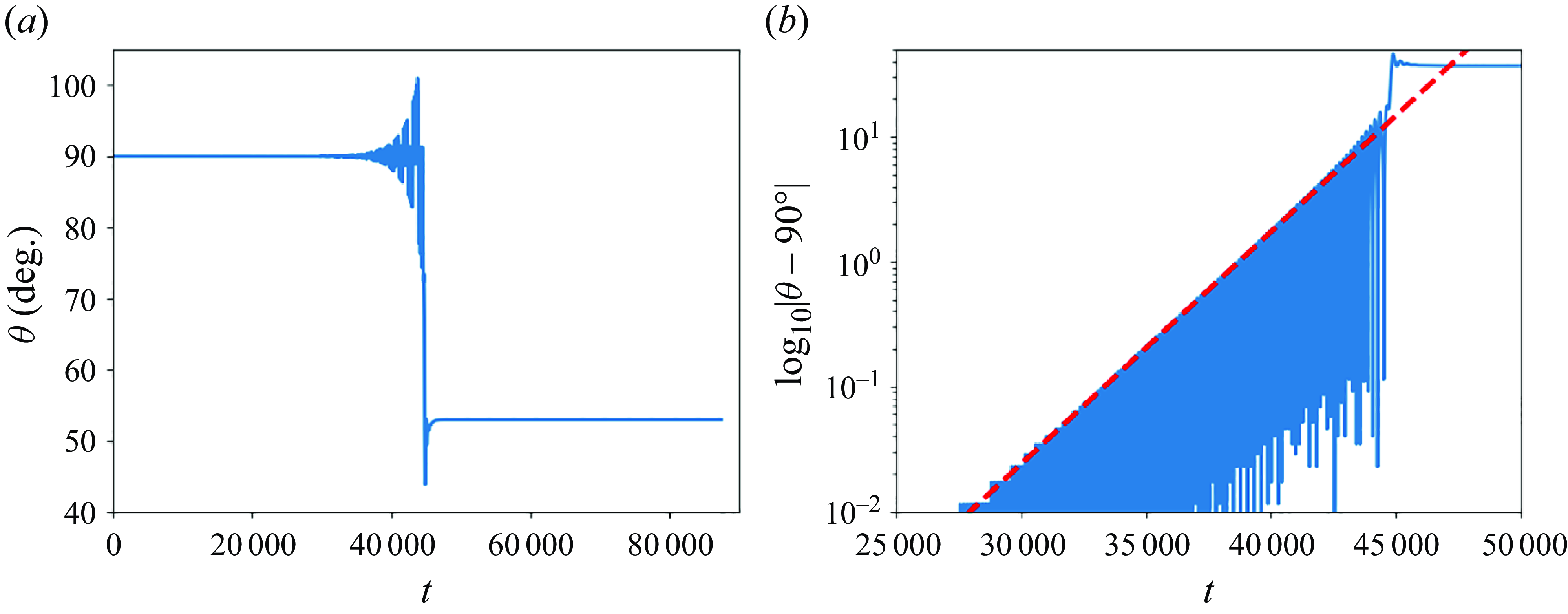
Figure 15. Dependence of $\theta$
on time for the non-planar initial configuration and an exemplary value
$\theta$
on time for the non-planar initial configuration and an exemplary value $B=12\,558$
. (a) The transient frozen rotating dynamics of the loop is observed until
$B=12\,558$
. (a) The transient frozen rotating dynamics of the loop is observed until $t \approx 30\,000$
followed by a slowly growing destabilisation until
$t \approx 30\,000$
followed by a slowly growing destabilisation until $t \approx 45\,000$
when the tilted mode is formed. (b) The amplitude
$t \approx 45\,000$
when the tilted mode is formed. (b) The amplitude $A_o$
of the oscillations of
$A_o$
of the oscillations of $\theta$
in the destabilisation stage is well-approximated by the exponential increase given by (4.1) with
$\theta$
in the destabilisation stage is well-approximated by the exponential increase given by (4.1) with $\lambda = 4.28 \times 10^{-4}$
, shown as the straight dashed line.
$\lambda = 4.28 \times 10^{-4}$
, shown as the straight dashed line.
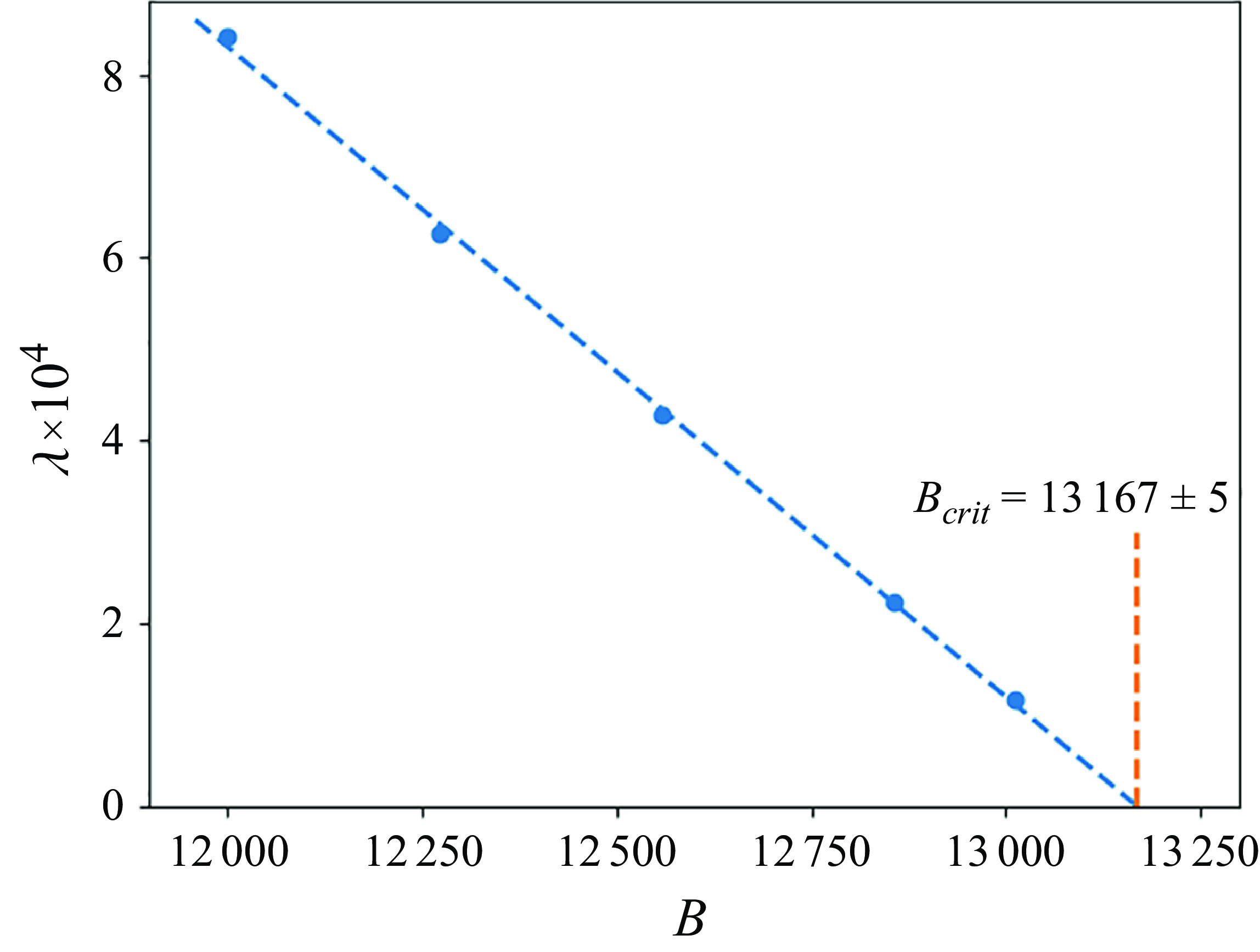
Figure 16. The growth rate $\lambda$
in (4.1) is a linear function of
$\lambda$
in (4.1) is a linear function of $B$
, enabling estimation of
$B$
, enabling estimation of $B_{crit}$
= 13 167 for the transition between the frozen rotating and tilted modes.
$B_{crit}$
= 13 167 for the transition between the frozen rotating and tilted modes.
Interestingly, for the lower range of the elasto-gravitation number, $12\,000 \leqslant B \leqslant 13\,138$
, in a very long first stage of the evolution, the loop seems to be in a frozen rotating mode (like it happens in the range of larger values of
$12\,000 \leqslant B \leqslant 13\,138$
, in a very long first stage of the evolution, the loop seems to be in a frozen rotating mode (like it happens in the range of larger values of $B$
); however, such behaviour is transient, and finally the tilted mode is reached.
$B$
); however, such behaviour is transient, and finally the tilted mode is reached.
To estimate the critical value $B_{crit}$
of the transition between the final tilted and frozen rotating modes, approached from the non-planar initial configuration, the evolution
$B_{crit}$
of the transition between the final tilted and frozen rotating modes, approached from the non-planar initial configuration, the evolution $\theta (t)$
is studied for the cases in which the frozen rotating transient destabilises if starting from the non-planar initial configuration. An example of this analysis is shown in figure 15 for
$\theta (t)$
is studied for the cases in which the frozen rotating transient destabilises if starting from the non-planar initial configuration. An example of this analysis is shown in figure 15 for $B=12\,558$
. It is seen that
$B=12\,558$
. It is seen that $\theta \approx 90^\circ$
for a while, but after the transition period, the loop continues to sediment in the tilted mode.
$\theta \approx 90^\circ$
for a while, but after the transition period, the loop continues to sediment in the tilted mode.
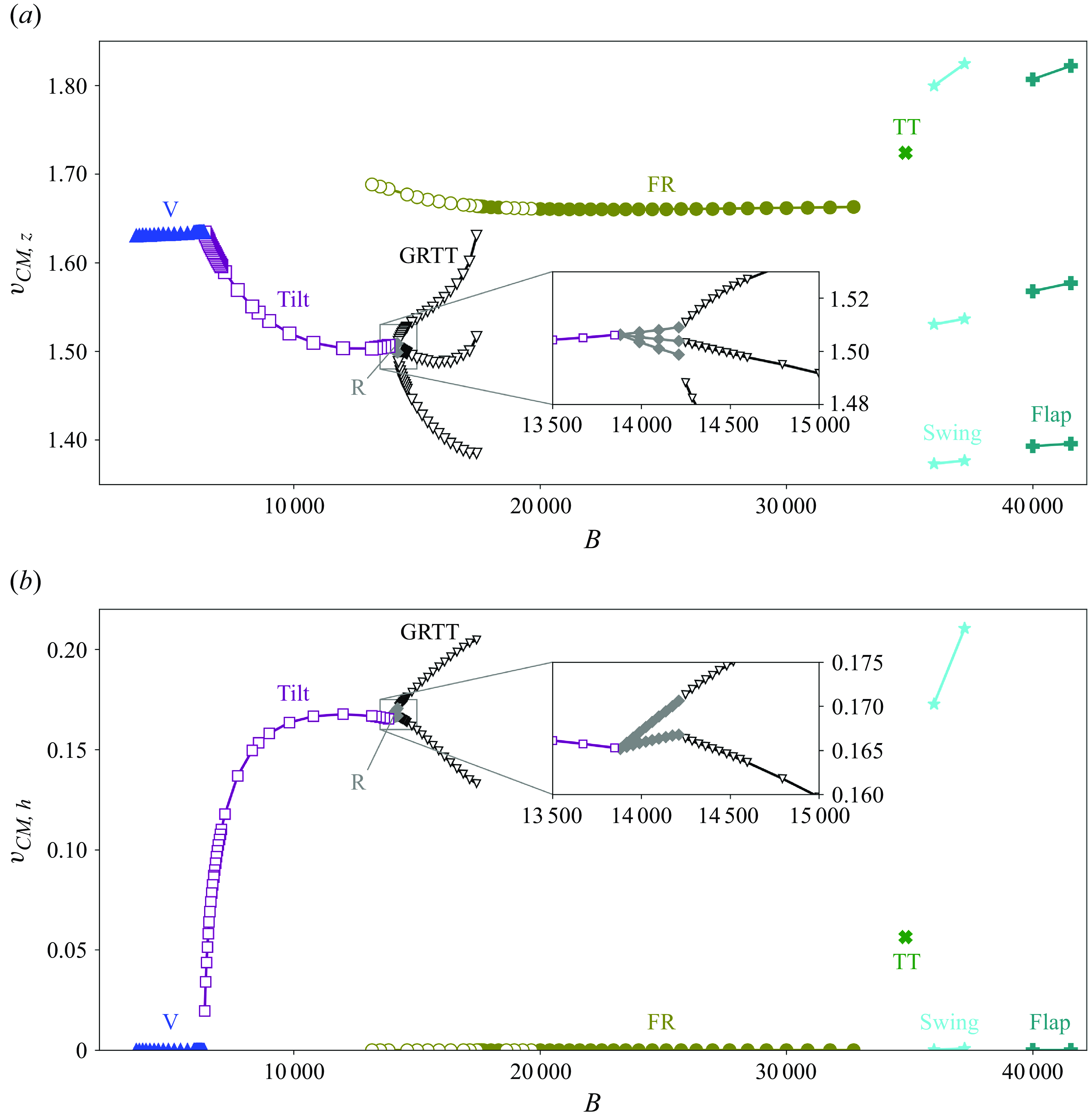
Figure 17. (a) The sedimentation speed $v_{CM,z}\gt 0$
and (b) the lateral speed
$v_{CM,z}\gt 0$
and (b) the lateral speed $v_{CM,h}\geqslant 0$
of the loop centre-of-mass as a function of elasto-gravitation number
$v_{CM,h}\geqslant 0$
of the loop centre-of-mass as a function of elasto-gravitation number $B$
. For the rocking, GRTT, swinging and flapping modes, the maximum and minimum of both velocities (and the average of
$B$
. For the rocking, GRTT, swinging and flapping modes, the maximum and minimum of both velocities (and the average of $v_{CM,z}$
) are shown. In the vertical, tilted, frozen rotating and tank-treading modes, both velocities do not depend on time. The colours and symbols correspond to the modes as presented in figures 12 and 13 for the planar and non-planar initial configurations, respectively.
$v_{CM,z}$
) are shown. In the vertical, tilted, frozen rotating and tank-treading modes, both velocities do not depend on time. The colours and symbols correspond to the modes as presented in figures 12 and 13 for the planar and non-planar initial configurations, respectively.
The initial stage of destabilisation can be analysed via the dependence of $\theta$
on time. The time-dependent amplitude
$\theta$
on time. The time-dependent amplitude $A_o(t)$
of the oscillations of
$A_o(t)$
of the oscillations of $\theta$
around
$\theta$
around $90 ^\circ$
can be approximated to increase exponentially,
$90 ^\circ$
can be approximated to increase exponentially,
 \begin{equation} A_o(t) \propto e^{\lambda t} \end{equation}
in the range $12\,000 \leqslant B \leqslant 13\,012$
. The dependence of
$12\,000 \leqslant B \leqslant 13\,012$
. The dependence of $\lambda \gt 0$
on
$\lambda \gt 0$
on $B$
is linear, allowing identification of the value of
$B$
is linear, allowing identification of the value of $B_{crit} \approx 13\,167$
below which the frozen rotating mode is not reached after a long time, as illustrated in figure 16.
$B_{crit} \approx 13\,167$
below which the frozen rotating mode is not reached after a long time, as illustrated in figure 16.
5. Centre-of-mass velocity and characteristic time scales for the attracting modes
In figure 17, we compare the characteristic centre-of-mass (CM) velocity of the elastic loop made of 36 spherical beads in different attracting modes. In figures 17(
a) and 17(b), we show separately the absolute values of the vertical and horizontal components of the CM velocity, $v_{CM,z}=|v_{z,c}|$
(in the following called the sedimentation speed) and
$v_{CM,z}=|v_{z,c}|$
(in the following called the sedimentation speed) and $v_{CM,h} = \sqrt {v_{CM,x}^{2} + v_{CM,y}^{2} }$
(called the lateral speed). The chosen normalisation, given in (2.8), is such that the sedimentation speed of a single bead is equal to
$v_{CM,h} = \sqrt {v_{CM,x}^{2} + v_{CM,y}^{2} }$
(called the lateral speed). The chosen normalisation, given in (2.8), is such that the sedimentation speed of a single bead is equal to $1/3$
.
$1/3$
.
The main observation is that the sedimentation speed is typically at least an order of magnitude larger than the lateral one. There is no horizontal drift in the vertical, frozen rotating and flapping modes. The lateral speed $v_{CM,h}$
is constant in time for the tank-treading and tilted modes. In the tilted mode, the horizontal drift tends to vanish when
$v_{CM,h}$
is constant in time for the tank-treading and tilted modes. In the tilted mode, the horizontal drift tends to vanish when $B$
decreases to the critical value corresponding to the transition between the tilted and vertical modes. In the tilted mode, the horizontal component of the CM velocity has a fixed direction, and in the tank-treading mode, the horizontal component of the CM velocity corresponds to the motion along a circle.
$B$
decreases to the critical value corresponding to the transition between the tilted and vertical modes. In the tilted mode, the horizontal component of the CM velocity has a fixed direction, and in the tank-treading mode, the horizontal component of the CM velocity corresponds to the motion along a circle.
In the rocking mode, the horizontal component of the CM velocity has a fixed direction plus oscillations along this direction and oscillations perpendicular to it. In the swinging mode, the horizontal component of the CM velocity has a fixed direction plus oscillations along this direction. In the GRTT mode, the horizontal component of the CM velocity corresponds to the motion along a circle plus periodic oscillations along the circle and perpendicular to it. The magnitude of the oscillations about the mean values in the rocking and GRTT modes increases with $B$
, seen as the increase in the difference between the maximum and minimum values of the sedimentation and lateral speeds. The characteristic time of the oscillations between the minimum and maximum sedimentation and lateral speeds for GRTT corresponds to
$B$
, seen as the increase in the difference between the maximum and minimum values of the sedimentation and lateral speeds. The characteristic time of the oscillations between the minimum and maximum sedimentation and lateral speeds for GRTT corresponds to $T_r$
shown in figure 6.
$T_r$
shown in figure 6.
For the rocking and GRTT modes, the lateral speed $v_{CM,h}= \sqrt {v_{CM,x}^{2} + v_{CM,y}^{2} }$
(i.e. the magnitude of the instantaneous horizontal velocity of the loop centre-of-mass) differs from the speed of the effective displacement of the loop centre of mass, i.e. from the gyration velocity
$v_{CM,h}= \sqrt {v_{CM,x}^{2} + v_{CM,y}^{2} }$
(i.e. the magnitude of the instantaneous horizontal velocity of the loop centre-of-mass) differs from the speed of the effective displacement of the loop centre of mass, i.e. from the gyration velocity $ v_g$
in the GRTT mode (shown in figure 9
b) and the horizontal drift velocity
$ v_g$
in the GRTT mode (shown in figure 9
b) and the horizontal drift velocity $v_{x,c}$
in the rocking mode (shown in figure 7). The gyration velocity
$v_{x,c}$
in the rocking mode (shown in figure 7). The gyration velocity $ v_g=A_g\,\omega _g$
, where
$ v_g=A_g\,\omega _g$
, where $A_{g}$
is the averaged radius of the gyrating motion and
$A_{g}$
is the averaged radius of the gyrating motion and $\omega _g$
is the vertical angular velocity, see (3.6). The horizontal drift velocity
$\omega _g$
is the vertical angular velocity, see (3.6). The horizontal drift velocity $v_{x.c}$
is defined in (3.5).
$v_{x.c}$
is defined in (3.5).
The dependence of the sedimentation and lateral speeds on $B$
is non-monotonic and very complex. The loop shape and orientation, and their variation with time, are essential for the resulting value and direction of the CM velocity. There is no systematic dependence of the lateral speed on
$B$
is non-monotonic and very complex. The loop shape and orientation, and their variation with time, are essential for the resulting value and direction of the CM velocity. There is no systematic dependence of the lateral speed on $B$
. The sedimentation speed of the loop with a fixed shape in the tank-treading mode is larger than in the frozen rotating mode, in the frozen rotating mode – larger than in the vertical mode, and in the vertical mode – larger than in the tilted mode. The last inequality is in agreement with the behaviour of an inclined rigid circle that sediments faster than a vertical circle of the same diameter.
$B$
. The sedimentation speed of the loop with a fixed shape in the tank-treading mode is larger than in the frozen rotating mode, in the frozen rotating mode – larger than in the vertical mode, and in the vertical mode – larger than in the tilted mode. The last inequality is in agreement with the behaviour of an inclined rigid circle that sediments faster than a vertical circle of the same diameter.
For the vertical, tilted and frozen rotating modes, the shape of the elastic loop is fixed in time, only translating or rotating and translating. We checked that the sedimentation speeds are practically the same as for the rigid particles of the same shape and orientation (a slight numerical difference is less than 0.2 %). However, the sedimentation speed of the elastic loop in the tank-treading mode is by 3.7 % larger than the sedimentation speed of the rigid loop of the same shape and orientation. This is consistent with the previous observations by Ekiel-Jeżewska & Wajnryb (Reference Ekiel-Jeżewska and Wajnryb2009a ) that the relative motion of certain parts of an object without a change of its shape leads to a higher sedimentation velocity than for the rigid object. Moreover, the calculation performed for the rigid object of the shape and orientation taken from the tank-treading mode shows that the horizontal components of the angular velocity do not vanish, and therefore its orientation is not stationary, unlike in the case of an elastic object, that rotates only along the vertical axis and moves along a circular helix. Clearly, the tank-treading motion stabilises the loop orientation, and the rigid body dynamics is different.
For a mode with a time-dependent shape deformation, variations in time of the sedimentation speed can be as large as 30% (as for example in the swinging mode). In general, it might be expected that almost horizontal loop (with a smaller value of $\theta$
) sediments slower than almost inclined loop (with a greater value of
$\theta$
) sediments slower than almost inclined loop (with a greater value of $\theta$
), and therefore, that the lower and upper branches in figure 17 (the minima and maxima of
$\theta$
), and therefore, that the lower and upper branches in figure 17 (the minima and maxima of $v_{CM,z}(t)$
over time) correspond to the lower and upper branches in figure 18(a) (the minima and maxima of
$v_{CM,z}(t)$
over time) correspond to the lower and upper branches in figure 18(a) (the minima and maxima of $\theta (t)$
), respectively. Indeed, for the rocking mode, the time positions of
$\theta (t)$
), respectively. Indeed, for the rocking mode, the time positions of $\theta _{max}$
and
$\theta _{max}$
and $\theta _{min}$
coincide with the time positions of the maximum and minimum values of
$\theta _{min}$
coincide with the time positions of the maximum and minimum values of $v_{CM,z}$
. For the GRTT and swinging modes, the values of the time at which
$v_{CM,z}$
. For the GRTT and swinging modes, the values of the time at which $\theta _{max}$
and
$\theta _{max}$
and $\theta _{min}$
are reached are close to the values of the time corresponding to the maximum and minimum values of
$\theta _{min}$
are reached are close to the values of the time corresponding to the maximum and minimum values of $v_{CM,z}$
. The reason for a small difference could be assigned to non-planar and non-circular shapes. For the flapping mode, the sedimentation speed is the smallest when the loop is almost horizontal.
$v_{CM,z}$
. The reason for a small difference could be assigned to non-planar and non-circular shapes. For the flapping mode, the sedimentation speed is the smallest when the loop is almost horizontal.
We now compare the characteristic time scales of the attracting modes, ordering them from the shortest to the longest. For all the modes, the smallest is the sedimentation time scale, of the order of 0.5–0.7. The time scale of the horizontal drift is $\gtrsim 5$
. The time scales of the rotation and tank-treading in the tank-treading mode are 50 and 100, of the flapping in the flapping mode, 150, of the rotation in the frozen rotating mode, 200–300, of the rocking in the rocking and GRTT modes and swinging in the swinging mode, around 300. Much longer are the gyration (1000–50 000) and tank-treading (4000–100 000) time scales in the GRTT mode. In general, the attracting modes are reached after a very long time.
$\gtrsim 5$
. The time scales of the rotation and tank-treading in the tank-treading mode are 50 and 100, of the flapping in the flapping mode, 150, of the rotation in the frozen rotating mode, 200–300, of the rocking in the rocking and GRTT modes and swinging in the swinging mode, around 300. Much longer are the gyration (1000–50 000) and tank-treading (4000–100 000) time scales in the GRTT mode. In general, the attracting modes are reached after a very long time.
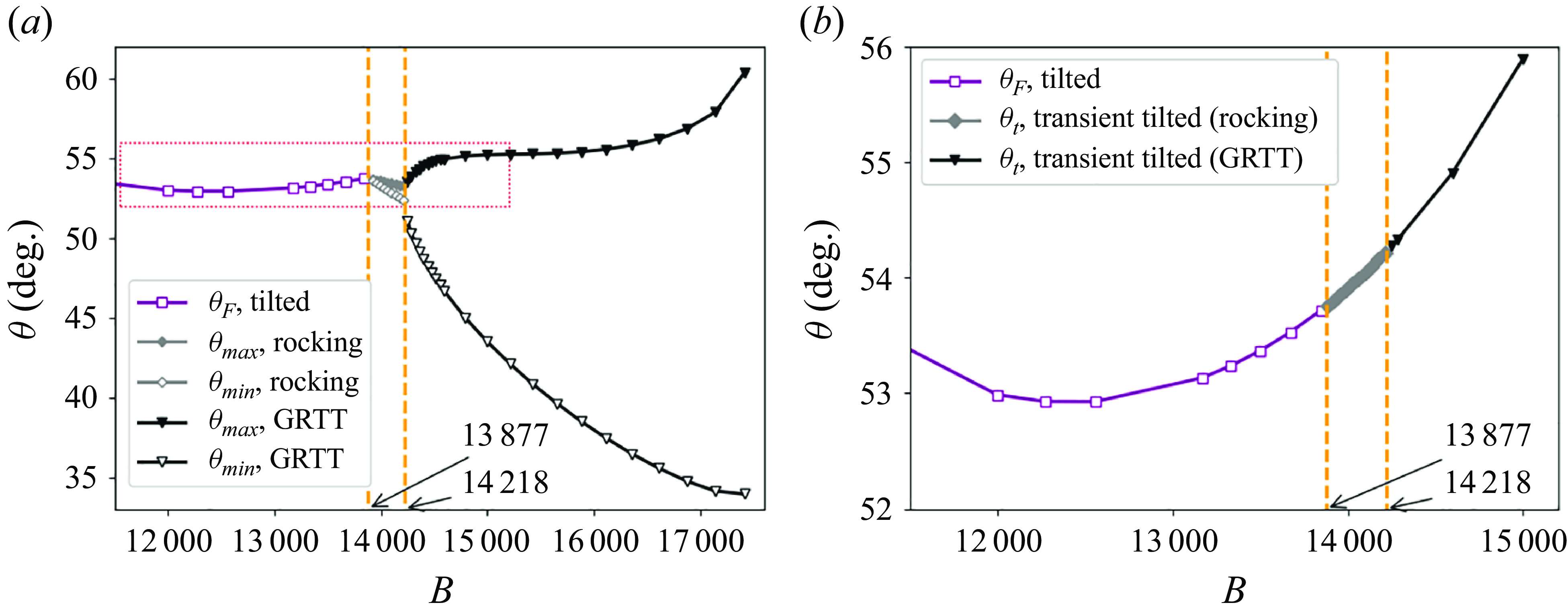
Figure 18. The polar angle $\theta$
of the loop as a function of the elasto-gravitation number
$\theta$
of the loop as a function of the elasto-gravitation number $B$
. (a) The final
$B$
. (a) The final $\theta _{F}$
for the tilted mode and maximum and minimum values of
$\theta _{F}$
for the tilted mode and maximum and minimum values of $\theta$
during the rocking and GRTT modes,
$\theta$
during the rocking and GRTT modes, $\theta _{max} = \theta _{0} + \theta _{2}$
and
$\theta _{max} = \theta _{0} + \theta _{2}$
and $\theta _{min} = \theta _{0} - \theta _{2}$
, see figures 4(a) and 5(a). (b) The polar angle for the attracting tilted mode (
$\theta _{min} = \theta _{0} - \theta _{2}$
, see figures 4(a) and 5(a). (b) The polar angle for the attracting tilted mode ( $\theta _{F}, \;B\le 13\,877$
) and for transient tilted configuration (
$\theta _{F}, \;B\le 13\,877$
) and for transient tilted configuration ( $\theta _{t}, \;12\,877\le B\le 15\,000$
) before the rocking and GRTT modes are established. The dashed rectangle in (a) corresponds to the axes limits used in (b).
$\theta _{t}, \;12\,877\le B\le 15\,000$
) before the rocking and GRTT modes are established. The dashed rectangle in (a) corresponds to the axes limits used in (b).
However, we numerically observe that in the first stage of the evolution, typically very long, the loop often behaves similarly as in such an attracting dynamical mode that is ‘close’ to the initial configuration, for example tilted for initially inclined circle and frozen rotating for the non-planar initial configuration, see figures 5 and 15(a), respectively. The averaged inclination angle $\theta _t$
of the transient tilted mode is shown in figure 18(b) as a function of
$\theta _t$
of the transient tilted mode is shown in figure 18(b) as a function of $B \geqslant 13\,877$
. It is clear that in this range of
$B \geqslant 13\,877$
. It is clear that in this range of $B$
, the function
$B$
, the function $\theta _t(B)$
for the transient configuration extends smoothly the function
$\theta _t(B)$
for the transient configuration extends smoothly the function $\theta _F(B)$
corresponding to the stable stationary configuration with
$\theta _F(B)$
corresponding to the stable stationary configuration with $B\le 13\,877$
. This similarity illustrates that the typical CM velocities and time scales analysed above for the attracting modes can be also observed at much shorter times as characteristic features of the transients.
$B\le 13\,877$
. This similarity illustrates that the typical CM velocities and time scales analysed above for the attracting modes can be also observed at much shorter times as characteristic features of the transients.
6. Discussion and conclusions
In our numerical findings, all the stationary configurations of the highly elastic loops are non-planar except the vertical one. This result differs from the known fact that all configurations of rigid circles are stationary – they translate vertically and horizontally with no change in their inclination angle, and are neutrally stable, as the sedimenting rods (Taylor Reference Taylor1967).
Now we will argue that there are no planar circular stationary configurations for an elastic loop made of $N$
beads, with the inclination angle
$N$
beads, with the inclination angle $\theta$
other than
$\theta$
other than $0^\circ$
(horizontal). Assume that there is one, which means that the velocity vector
$0^\circ$
(horizontal). Assume that there is one, which means that the velocity vector $\boldsymbol{v}_i$
of each bead
$\boldsymbol{v}_i$
of each bead $i=1,\ldots ,N$
is the same. The vectors
$i=1,\ldots ,N$
is the same. The vectors $\boldsymbol{v}_i$
are sums of two contributions:
$\boldsymbol{v}_i$
are sums of two contributions: $\boldsymbol{v}_i^{\perp }$
, caused by the forces (acting on all the beads
$\boldsymbol{v}_i^{\perp }$
, caused by the forces (acting on all the beads $j=1,\ldots ,N$
) perpendicular to the circle, and
$j=1,\ldots ,N$
) perpendicular to the circle, and $\boldsymbol{v}_i^{\parallel }$
caused by the forces (acting on all the beads
$\boldsymbol{v}_i^{\parallel }$
caused by the forces (acting on all the beads $j=1,\ldots ,N$
) parallel to the circle. The forces perpendicular to the circle are only the perpendicular components of gravity, while the parallel ones are the parallel components of gravity plus all the elastic forces. Owing to symmetry,
$j=1,\ldots ,N$
) parallel to the circle. The forces perpendicular to the circle are only the perpendicular components of gravity, while the parallel ones are the parallel components of gravity plus all the elastic forces. Owing to symmetry, $\boldsymbol{v}_i^{\perp }$
is perpendicular, and
$\boldsymbol{v}_i^{\perp }$
is perpendicular, and $\boldsymbol{v}_i^{\parallel }$
is parallel to the circle; moreover,
$\boldsymbol{v}_i^{\parallel }$
is parallel to the circle; moreover, $\boldsymbol{v}_i^{\perp }$
is the same for all the beads
$\boldsymbol{v}_i^{\perp }$
is the same for all the beads $i$
.
$i$
.
To require that the vector $\boldsymbol{v}_i^{\parallel }$
is also the same for all the beads, we need to select the circle in the elastic equilibrium (with vanishing elastic forces). In particular, for the horizontal circle (i.e. for
$\boldsymbol{v}_i^{\parallel }$
is also the same for all the beads, we need to select the circle in the elastic equilibrium (with vanishing elastic forces). In particular, for the horizontal circle (i.e. for $\theta =0$
) in the elastic equilibrium, no horizontal forces are acting on each bead
$\theta =0$
) in the elastic equilibrium, no horizontal forces are acting on each bead $i$
; therefore, this configuration is stationary. In general,
$i$
; therefore, this configuration is stationary. In general, $\theta \ne 0$
, and the only parallel force acting on a bead
$\theta \ne 0$
, and the only parallel force acting on a bead $i$
is the parallel component of gravity,
$i$
is the parallel component of gravity, $F=G/N \sin \theta \ne 0$
. We consider
$F=G/N \sin \theta \ne 0$
. We consider $N=36$
for simplicity and assume that beads 1 and 19 are at the bottom and at the top, respectively, and the line of centres of beads 10 and 28 is horizontal. Numerical evaluation of
$N=36$
for simplicity and assume that beads 1 and 19 are at the bottom and at the top, respectively, and the line of centres of beads 10 and 28 is horizontal. Numerical evaluation of $\boldsymbol{v}_i^{\parallel }$
demonstrates that
$\boldsymbol{v}_i^{\parallel }$
demonstrates that $|\boldsymbol{v}_{10}^{\parallel }|\gt |\boldsymbol{v}_1^{\parallel }|$
by around 6 %, in a qualitative agreement with analytical predictions based on the point-force model (the details are given in Appendix C). Therefore, a circle is not a stationary configuration, except if it is oriented horizontally. Our numerical analysis demonstrates that the stationary horizontal circular configuration is unstable, as shown in Appendix C.
$|\boldsymbol{v}_{10}^{\parallel }|\gt |\boldsymbol{v}_1^{\parallel }|$
by around 6 %, in a qualitative agreement with analytical predictions based on the point-force model (the details are given in Appendix C). Therefore, a circle is not a stationary configuration, except if it is oriented horizontally. Our numerical analysis demonstrates that the stationary horizontal circular configuration is unstable, as shown in Appendix C.
In the vertical attracting mode, a stationary non-circular planar (vertical) configuration is reached, shown in figure 25 in Appendix C, and also in figure 2 in (Gruziel-Słomka et al. Reference Gruziel-Słomka, Kondratiuk, Szymczak and Ekiel-Jeżewska2019). However, this configuration is not stationary if tilted – our numerical computations show that $\boldsymbol{v}_i^{\perp }$
is not the same for all the beads
$\boldsymbol{v}_i^{\perp }$
is not the same for all the beads $i$
(see Appendix C). These observations seem to indicate the non-existence of a planar stationary configuration of an elastic loop, except if oriented vertically or horizontally.
$i$
(see Appendix C). These observations seem to indicate the non-existence of a planar stationary configuration of an elastic loop, except if oriented vertically or horizontally.
The existence of attracting stationary and transient tilted and frozen rotating configurations is important for the overall structure of invariant manifolds of the dynamics, and their stability, as described, for example in Barenblatt (Reference Barenblatt1996). In future studies of the invariant manifolds and bifurcations of the dynamics of highly elastic loops (or fibres with open ends), the methods from Fox & Graham (Reference Fox and Graham2024) might be useful. In the future, it would also be interesting to understand the nature of the bifurcations between the different dynamical modes by a mathematical stability analysis, for example using the methods described by Clarke, Hwang & Keaveny (Reference Clarke, Hwang and Keaveny2024).
The existence of several attracting dynamical modes of highly elastic loops is similar to the existence of attracting modes of highly elastic fibres with open ends, described in Melikhov & Ekiel-Jeżewska (Reference Melikhov and Ekiel-Jeżewska2024). For both elastic objects, there exist two stationary shapes: one translating vertically and horizontally (called tilted) and one translating and rotating (called frozen rotating and rotation, respectively). Also, there exist modes oscillating periodically and quasiperiodically (the analogues of the rocking and GRTT modes for loops are, respectively, the crawling and rotation-crawling modes for the fibres). In general, the attracting modes are approached after a long time. However, the details of the shape evolution and centre-of-mass motion are different. In particular, for the same value of $B$
, the shapes of the loops are less deformed and closer to planar than for the fibres with open ends. Moreover, for the loops, the transition between different modes is shifted to much larger values of
$B$
, the shapes of the loops are less deformed and closer to planar than for the fibres with open ends. Moreover, for the loops, the transition between different modes is shifted to much larger values of $B$
than for the fibres with open ends. For very large values of
$B$
than for the fibres with open ends. For very large values of $B$
, for the loops there are more different periodic attracting modes (tank-treading, swinging, flapping) than for the fibres with open ends, for which often irregular evolution is observed.
$B$
, for the loops there are more different periodic attracting modes (tank-treading, swinging, flapping) than for the fibres with open ends, for which often irregular evolution is observed.
In conclusion, the main results of this paper are as follows. Different attracting dynamical modes of a highly elastic loop sedimenting under gravity in a viscous fluid are observed for different values of the elasto-gravitation number $B$
, starting from planar and non-planar initial conditions. This work extends the study performed by Gruziel-Słomka et al. (Reference Gruziel-Słomka, Kondratiuk, Szymczak and Ekiel-Jeżewska2019) as outlined in Appendix D. Two new modes of the dynamics is described: rocking and GRTT, and it is shown that (as the tilted mode) they can coexist with the frozen rotating mode for certain values of
$B$
, starting from planar and non-planar initial conditions. This work extends the study performed by Gruziel-Słomka et al. (Reference Gruziel-Słomka, Kondratiuk, Szymczak and Ekiel-Jeżewska2019) as outlined in Appendix D. Two new modes of the dynamics is described: rocking and GRTT, and it is shown that (as the tilted mode) they can coexist with the frozen rotating mode for certain values of $B$
. Critical values of
$B$
. Critical values of $B$
corresponding to transitions between all the attracting modes are determined. Beyond the transition, some of the modes become unstable (but still can be observed), while others cease to exist. For each attracting mode, characteristic time scales are evaluated. Sedimentation and lateral translational velocities, and the angular velocity are calculated and shown to vary depending on the mode and the value of the elasto-gravitation number.
$B$
corresponding to transitions between all the attracting modes are determined. Beyond the transition, some of the modes become unstable (but still can be observed), while others cease to exist. For each attracting mode, characteristic time scales are evaluated. Sedimentation and lateral translational velocities, and the angular velocity are calculated and shown to vary depending on the mode and the value of the elasto-gravitation number.
We will now comment on possible practical significance of the dynamics of sedimenting highly elastic loops. Moderately elongated biological objects are typically characterised by values of $B\lesssim 200$
. Their density is close to unity, and therefore, the total force (gravity minus buoyancy) is relatively small. This, however, could be compensated by a large length. For example, the estimated value of the elasto-gravitation number for a diatom chain of diameter
$B\lesssim 200$
. Their density is close to unity, and therefore, the total force (gravity minus buoyancy) is relatively small. This, however, could be compensated by a large length. For example, the estimated value of the elasto-gravitation number for a diatom chain of diameter $d = 20\,{\unicode{x03BC} {\rm m}}$
, density
$d = 20\,{\unicode{x03BC} {\rm m}}$
, density $\rho = 1125\,\rm kg\, m^{-3}$
, chain bending stiffness
$\rho = 1125\,\rm kg\, m^{-3}$
, chain bending stiffness $A = 1.3 \times 10^{-17}$
and length
$A = 1.3 \times 10^{-17}$
and length $2~{\rm mm}$
corresponds to
$2~{\rm mm}$
corresponds to $B = 200$
, as reported by Young et al. (Reference Young, Karp-Boss, Jumars and Landis2012) and Bukowicki & Ekiel-Jeżewska (Reference Bukowicki and Ekiel-Jeżewska2019). The range of values of
$B = 200$
, as reported by Young et al. (Reference Young, Karp-Boss, Jumars and Landis2012) and Bukowicki & Ekiel-Jeżewska (Reference Bukowicki and Ekiel-Jeżewska2019). The range of values of $B$
considered in our manuscript would be reached for longer,
$B$
considered in our manuscript would be reached for longer, $6-12~{\rm mm}$
-long diatom chains, closed in a loop.
$6-12~{\rm mm}$
-long diatom chains, closed in a loop.
Moreover, the highly elastic loops investigated here could be considered as a model of a very thin elastic sheet. The dynamics of such objects have been recently investigated because of their possible application for graphene flakes. Young’s modulus of graphene is very large, around $1\;TPa$
, but owing to minimal thickness, the bending rigidity of monolayer graphene is very low, of the order of
$1\;TPa$
, but owing to minimal thickness, the bending rigidity of monolayer graphene is very low, of the order of $1\;eV$
, see, for example Berinskii, Krivtsov & Kudarova (Reference Berinskii, Krivtsov and Kudarova2014). Moreover, graphene’s density is large, equal to 2267
$1\;eV$
, see, for example Berinskii, Krivtsov & Kudarova (Reference Berinskii, Krivtsov and Kudarova2014). Moreover, graphene’s density is large, equal to 2267 $\rm kg\, m^{-3}$
, with the density relative to the water-based solvent one order of magnitude larger than for biological systems like diatom chains.
$\rm kg\, m^{-3}$
, with the density relative to the water-based solvent one order of magnitude larger than for biological systems like diatom chains.
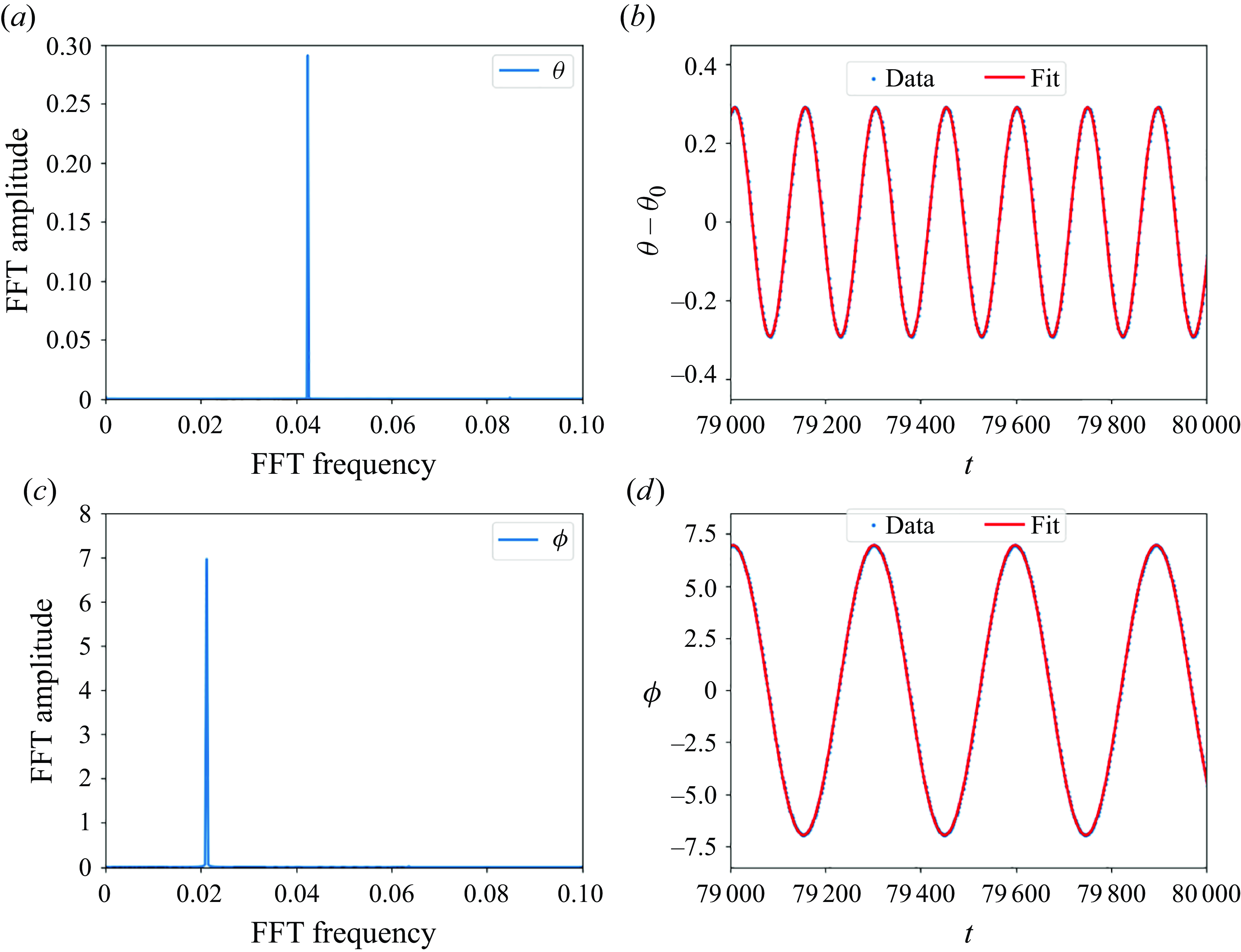
Figure 19. Fitting the time dependence given by (3.4) to the numerical data for the orientation angles $\theta$
and
$\theta$
and $\phi$
in the rocking mode with
$\phi$
in the rocking mode with $B=14\,098$
. (a,c) The FFT analysis of
$B=14\,098$
. (a,c) The FFT analysis of $\theta$
and
$\theta$
and $\phi$
. (b) The fit of
$\phi$
. (b) The fit of $\theta -\theta _0$
is performed with one dominant FFT frequency
$\theta -\theta _0$
is performed with one dominant FFT frequency $2 \omega _r$
. (d) The fit of
$2 \omega _r$
. (d) The fit of $\phi$
is performed with one dominant FFT frequency
$\phi$
is performed with one dominant FFT frequency $\omega _r$
.
$\omega _r$
.
The differences between the sedimentation velocities of the elastic loops in different modes determined here might be used in a centrifuge to sort the loops with different densities, different lengths or different elastoviscous numbers. A similar sorting of elastic fibres with open ends can be expected, based on the results shown in figure 5(d) in (Melikhov & Ekiel-Jeżewska Reference Melikhov and Ekiel-Jeżewska2024). The horizontal translation in a single direction of the sedimenting elastic loop for the tilted and rocking modes could be relevant for transporting cargo, and the motion of the loop centre-of-mass along a horizontal circle, and the oscillations of the centre-of-mass position might be useful for mixing of the fluid. The dynamics of highly elastic loops and fibres may be useful to explain the motion and shape deformation of more complex highly elastic objects, for example disks or sheets (Miara et al. Reference Miara, Juel, Pihler-Puzovic and Heil2022; Yu & Graham Reference Yu and Graham2024).
Supplementary movies
Supplementary movies are available at https://doi.org/10.1017/jfm.2025.10203.
Acknowledgements
We thank M. Gruziel-Słomka, P. Szymczak, M. Lisicki and R. Waszkiewicz for helpful discussions.
Funding
This work was supported in part by the National Science Centre under grant UMO-2021/41/B/ST8/04474.
Declaration of interests
The authors report no conflict of interest.
Data availability statement
The data that support the findings of this study are openly available in RepOD – Repository for Open Data at https://doi.org/10.18150/IOI0RG.
Appendix A. Fitting expressions
For the rocking and GRTT modes, we perform the fast Fourier transform (FFT) of the numerical data for the time-dependent orientation angles $\theta$
and
$\theta$
and $\phi$
and the centre-of-mass position
$\phi$
and the centre-of-mass position $(x_{CM},\,y_{CM},\,z_{CM})$
and we determine the leading frequencies. Then, we use these values to construct and plot the fitting expressions.
$(x_{CM},\,y_{CM},\,z_{CM})$
and we determine the leading frequencies. Then, we use these values to construct and plot the fitting expressions.
The results of the FFT analysis of the data and the fitting expressions for the rocking mode with $B=14\,098$
are shown in figures 19 and 20. The parameters are
$B=14\,098$
are shown in figures 19 and 20. The parameters are $\theta _0 = 53 ^\circ$
,
$\theta _0 = 53 ^\circ$
, $\omega _r = 2.12 \times 10^{-2}$
,
$\omega _r = 2.12 \times 10^{-2}$
, $v_{x,c} = 0.166$
and
$v_{x,c} = 0.166$
and $v_{z,c} = 1.505$
.
$v_{z,c} = 1.505$
.
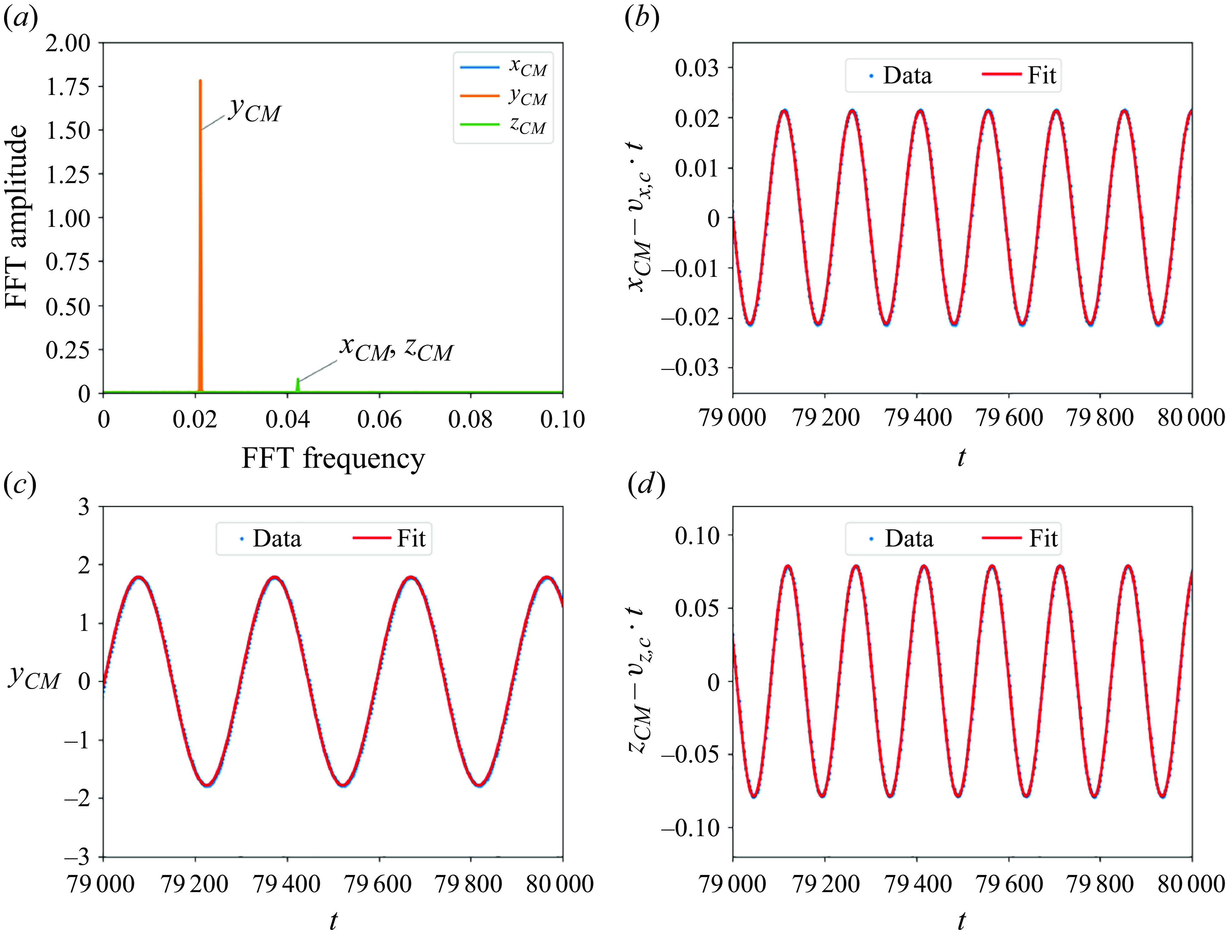
Figure 20. The centre-of-mass movement for the rocking mode with $B=14\,098$
. (a) The FFT of
$B=14\,098$
. (a) The FFT of $x_{CM}$
,
$x_{CM}$
, $y_{CM}$
and
$y_{CM}$
and $z_{CM}$
. (b–d) The fits of quasiperiodic
$z_{CM}$
. (b–d) The fits of quasiperiodic $x_{CM}$
,
$x_{CM}$
, $y_{CM}$
and
$y_{CM}$
and $z_{CM}$
were performed with one dominant FFT frequency only:
$z_{CM}$
were performed with one dominant FFT frequency only: $\omega _{r}$
for
$\omega _{r}$
for $y_{CM}$
, and
$y_{CM}$
, and $2 \omega _{r}$
for
$2 \omega _{r}$
for $x_{CM}$
and
$x_{CM}$
and $z_{CM}$
. The amplitudes are
$z_{CM}$
. The amplitudes are $0.0213$
,
$0.0213$
, $1.781$
and
$1.781$
and $0.079$
for
$0.079$
for $x_{CM}$
,
$x_{CM}$
, $y_{CM}$
and
$y_{CM}$
and $z_{CM}$
, respectively. See (3.5) for the fitting functions.
$z_{CM}$
, respectively. See (3.5) for the fitting functions.
The results of the FFT analysis of the data and the fitting expressions for the GRTT mode with $B=16362$
are shown in figures 21 and 22. Even though the amplitudes of the frequencies
$B=16362$
are shown in figures 21 and 22. Even though the amplitudes of the frequencies $\omega _r-\omega _g$
and
$\omega _r-\omega _g$
and $\omega _r+\omega _g$
are more than 30 times smaller than the amplitude of
$\omega _r+\omega _g$
are more than 30 times smaller than the amplitude of $\omega _g$
, they need to be taken into account to demonstrate the quasiperiodicity of
$\omega _g$
, they need to be taken into account to demonstrate the quasiperiodicity of $x_{CM}(t)$
and
$x_{CM}(t)$
and $y_{CM}(t)$
. The parameters are
$y_{CM}(t)$
. The parameters are $\theta _0 = 47 ^\circ$
,
$\theta _0 = 47 ^\circ$
, $\omega _g = 2.43 \cdot 10^{-3}$
,
$\omega _g = 2.43 \cdot 10^{-3}$
, $\omega _r = 2.30 \cdot 10^{-2}$
and
$\omega _r = 2.30 \cdot 10^{-2}$
and $v_{z,c} = 1.489$
.
$v_{z,c} = 1.489$
.
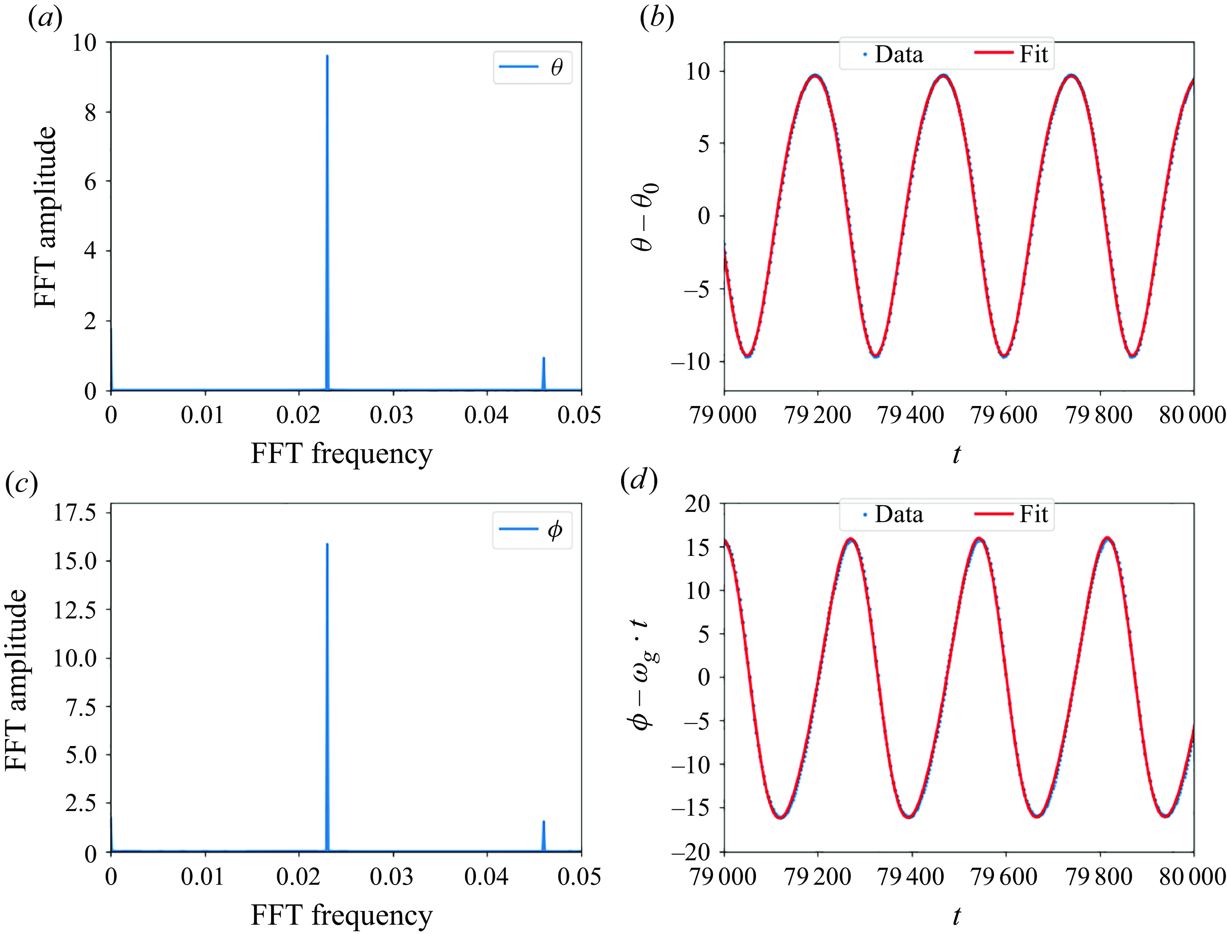
Figure 21. Fitting the time dependence given by (3.6) to the numerical data for the orientation angles $\theta$
and
$\theta$
and $\phi$
in the GRTT mode with
$\phi$
in the GRTT mode with $B=16\,362$
. (a,c) The FFT analysis of
$B=16\,362$
. (a,c) The FFT analysis of $\theta$
and
$\theta$
and $\phi$
. (b,d) The fits of
$\phi$
. (b,d) The fits of $\theta -\theta _0$
and
$\theta -\theta _0$
and $\phi -\omega _g t$
, performed with two dominant FFT frequencies,
$\phi -\omega _g t$
, performed with two dominant FFT frequencies, $\omega _r$
and
$\omega _r$
and $2\omega _r$
.
$2\omega _r$
.
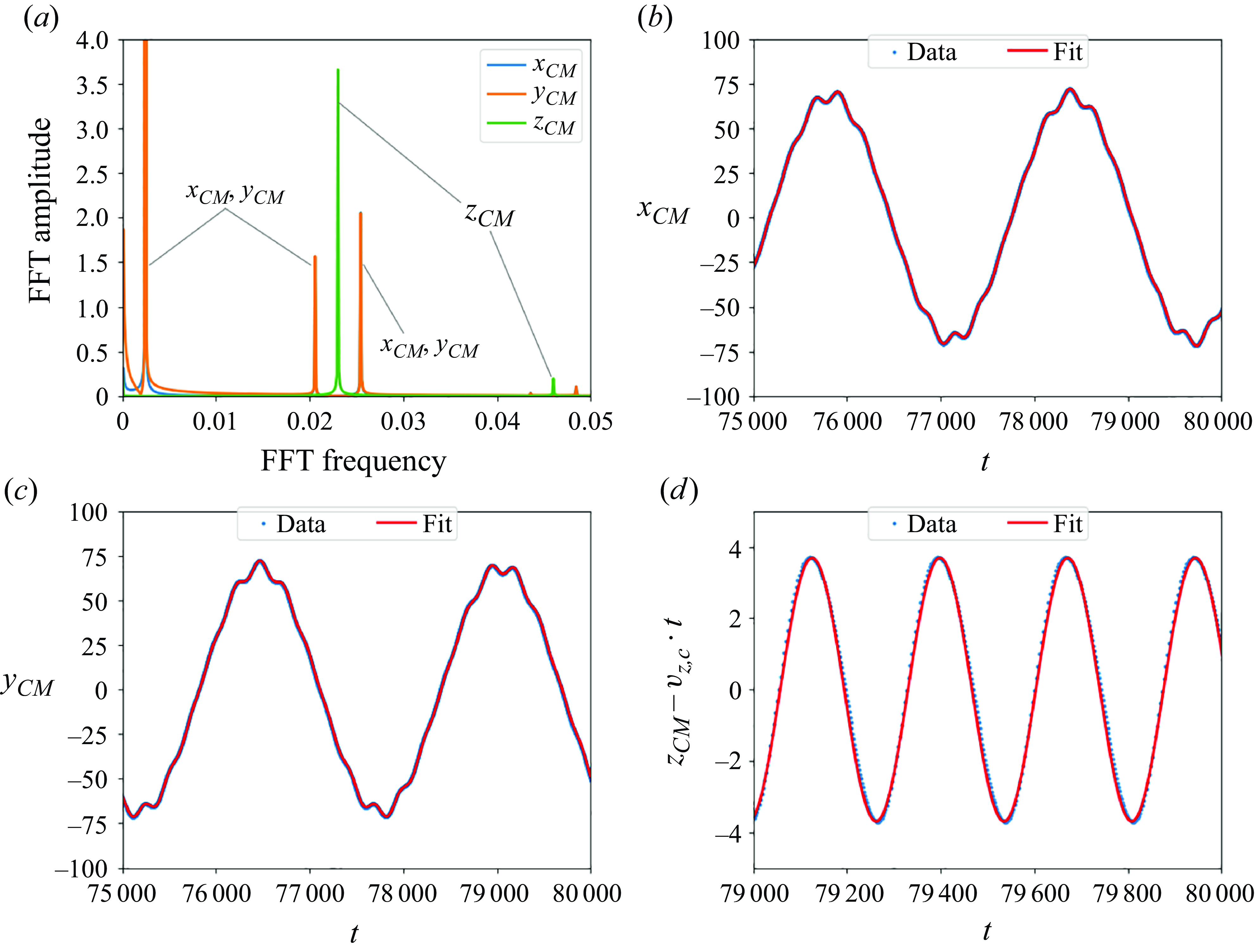
Figure 22. The centre-of-mass movement for the GRTT mode with $B=16\,362$
. (a) The FFT of
$B=16\,362$
. (a) The FFT of $x_{CM}$
,
$x_{CM}$
, $y_{CM}$
(overlapped) and
$y_{CM}$
(overlapped) and $z_{CM}$
. (b–c) The fit of quasiperiodic
$z_{CM}$
. (b–c) The fit of quasiperiodic $x_{CM}$
and
$x_{CM}$
and $y_{CM}$
was performed with three dominant FFT frequencies, and the amplitude of the first frequency, equal to
$y_{CM}$
was performed with three dominant FFT frequencies, and the amplitude of the first frequency, equal to $68.60$
, is truncated in the plot. (d) The fit of periodic
$68.60$
, is truncated in the plot. (d) The fit of periodic $z_{CM}-v_{z,c}t$
was performed with one FFT frequency only. See (3.7) for the fitting functions.
$z_{CM}-v_{z,c}t$
was performed with one FFT frequency only. See (3.7) for the fitting functions.
Appendix B. The critical value $\boldsymbol{B}_{\boldsymbol{crit}}$
for the transition between the rocking and GRTT modes
$\boldsymbol{B}_{\boldsymbol{crit}}$
for the transition between the rocking and GRTT modes

Figure 23 demonstrates that in the GRTT mode, when $B$
decreases to a critical value
$B$
decreases to a critical value $B_{crit}$
, the gyration period
$B_{crit}$
, the gyration period $T_g$
diverges as
$T_g$
diverges as $T_g \sim |B-B_{crit}|^{-\chi }$
, in agreement with (3.8). The fitting procedure was used to determine the critical value of
$T_g \sim |B-B_{crit}|^{-\chi }$
, in agreement with (3.8). The fitting procedure was used to determine the critical value of $B_{crit}$
. The range of
$B_{crit}$
. The range of $B$
for which this procedure was performed was limited to the closest data points near the expected
$B$
for which this procedure was performed was limited to the closest data points near the expected $B_{crit}$
:
$B_{crit}$
: $14\,248 \leqslant B \leqslant 14\,594$
(see figure 8
a). The best fit, which yielded the smallest residual, resulted in
$14\,248 \leqslant B \leqslant 14\,594$
(see figure 8
a). The best fit, which yielded the smallest residual, resulted in $\chi = -0.5560$
and
$\chi = -0.5560$
and $B_{crit} = 14\,218$
. For larger values, the GRTT mode is observed, and for smaller values, the rocking mode is present.
$B_{crit} = 14\,218$
. For larger values, the GRTT mode is observed, and for smaller values, the rocking mode is present.
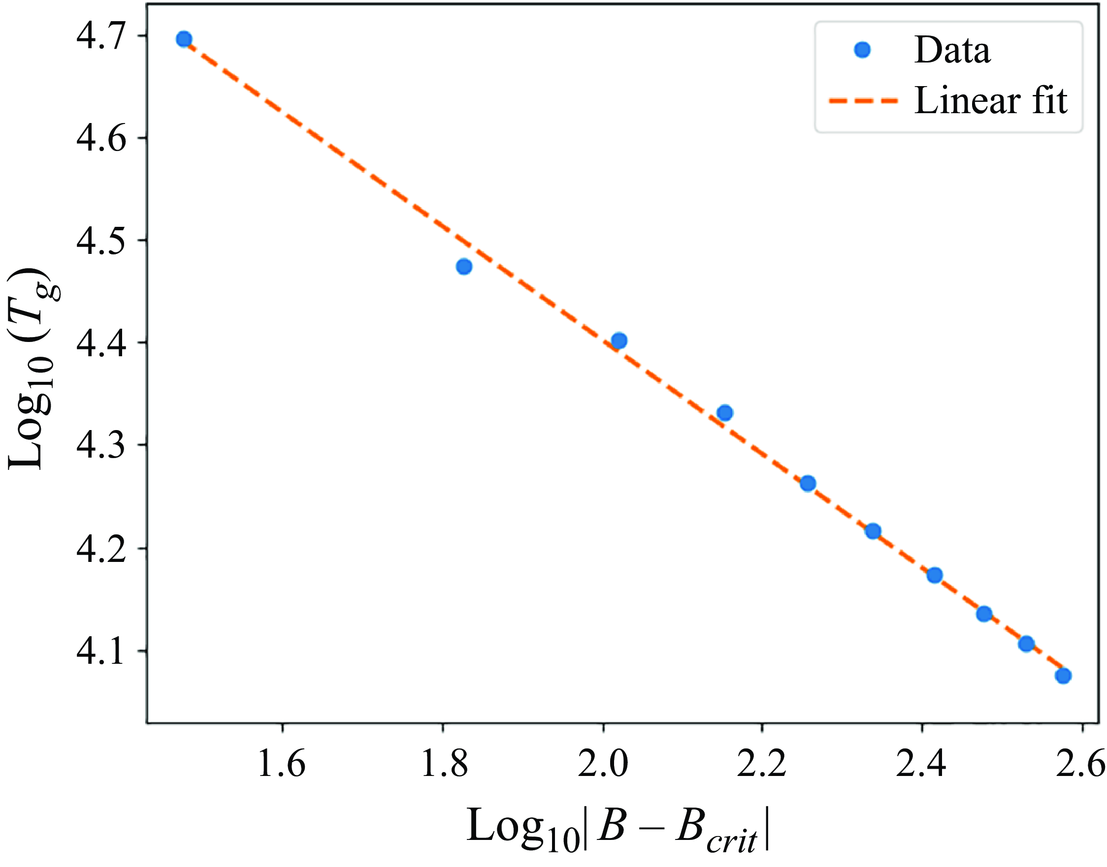
Figure 23. Log–log plot of the gyration period $T_{g}$
in the GRTT mode as a function of
$T_{g}$
in the GRTT mode as a function of $|B-B_{crit}|$
confirms a power law dependence (3.8) with the critical value
$|B-B_{crit}|$
confirms a power law dependence (3.8) with the critical value $B_{crit}=14\,218$
. The range of elasto-gravitation number
$B_{crit}=14\,218$
. The range of elasto-gravitation number $B$
chosen for the fit is
$B$
chosen for the fit is $14\,248 \leqslant B \leqslant 14\,594$
.
$14\,248 \leqslant B \leqslant 14\,594$
.
Appendix C. Examples of stationary and non-stationary planar configurations of a sedimenting elastic loop
A non-horizontal circle is not a stationary configuration (for all values of
$B$
)

First, we demonstrate that a vertical circle made of $N$
beads is not a stationary configuration, even if it is in elastic equilibrium. For
$N$
beads is not a stationary configuration, even if it is in elastic equilibrium. For $N=36$
, the beads 19 and 1 are at the top and bottom, respectively, and the line of centres of the beads 10 and 28 is horizontal. The numerically evaluated
$N=36$
, the beads 19 and 1 are at the top and bottom, respectively, and the line of centres of the beads 10 and 28 is horizontal. The numerically evaluated $i$
th bead velocities are shown in figure 24. The vertical component of the first and 19th bead velocity is smaller than for the 10th and 28th beads, by approximately 6 %. The horizontal component of velocity tends to move apart the upper beads and the lower beads closer to each other.
$i$
th bead velocities are shown in figure 24. The vertical component of the first and 19th bead velocity is smaller than for the 10th and 28th beads, by approximately 6 %. The horizontal component of velocity tends to move apart the upper beads and the lower beads closer to each other.
Therefore, the circular vertical configuration of the elastic loop is not stationary. This conclusion can be supported by an analytical calculation within the point-particle model. We will show that the sedimentation speed of the top bead is smaller than the sedimentation speed of the right-hand side bead, ${v}_{19}\lt {v}_{10}$
. The contribution to
${v}_{19}\lt {v}_{10}$
. The contribution to ${v}_{19}$
from four beads,
${v}_{19}$
from four beads, $19\!+\!k$
,
$19\!+\!k$
, $19\!-\!k$
, and their horizontal reflections,
$19\!-\!k$
, and their horizontal reflections, $1\!+\!k$
,
$1\!+\!k$
, $37\!-\!k$
, scaling as
$37\!-\!k$
, scaling as $v_k^v=\cos \phi _k + 1/\cos \phi _k + \sin \phi _k + 1/\sin \phi _k$
is smaller than the contribution to
$v_k^v=\cos \phi _k + 1/\cos \phi _k + \sin \phi _k + 1/\sin \phi _k$
is smaller than the contribution to ${v}_{10}$
from the analogous rotated configuration of four beads
${v}_{10}$
from the analogous rotated configuration of four beads $10\!+\!k$
,
$10\!+\!k$
, $10\!-\!k$
, and their vertical reflections,
$10\!-\!k$
, and their vertical reflections, $28\!+\!k$
,
$28\!+\!k$
, $28\!-\!k$
, scaling as
$28\!-\!k$
, scaling as $v_k^h=\sin ^2\phi _k/\cos \phi _k + 1/\cos \phi _k + \cos ^2\phi _k/\sin \phi _k + 1/\sin \phi _k$
, where
$v_k^h=\sin ^2\phi _k/\cos \phi _k + 1/\cos \phi _k + \cos ^2\phi _k/\sin \phi _k + 1/\sin \phi _k$
, where $k=1,\ldots ,8$
and
$k=1,\ldots ,8$
and $\phi _k= \pi (18-k)/36 \gt \pi /4$
. The contribution to
$\phi _k= \pi (18-k)/36 \gt \pi /4$
. The contribution to ${v}_{10}$
from the beads 1 and 19 is the same as the contribution
${v}_{10}$
from the beads 1 and 19 is the same as the contribution ${v}_{19}$
from the beads 10 and 28. The contribution to
${v}_{19}$
from the beads 10 and 28. The contribution to ${v}_{19}$
from the bead 1, scaling as
${v}_{19}$
from the bead 1, scaling as $1$
, is larger than the contribution to
$1$
, is larger than the contribution to ${v}_{10}$
from the bead 28, scaling as
${v}_{10}$
from the bead 28, scaling as $1/2$
, but it is easy to check that this difference is smaller than the difference
$1/2$
, but it is easy to check that this difference is smaller than the difference $v_1^h-v_1^v$
. Therefore, within the point-particle model,
$v_1^h-v_1^v$
. Therefore, within the point-particle model, ${v}_{19}\lt {v}_{10}$
.
${v}_{19}\lt {v}_{10}$
.
The reasoning presented above is generalised straightforwardly for an inclined circle other than horizontal – the vertical gravitational force needs to be replaced by its projection parallel to the circle’s plane. Therefore, a circle other than horizontal is not a stationary configuration.
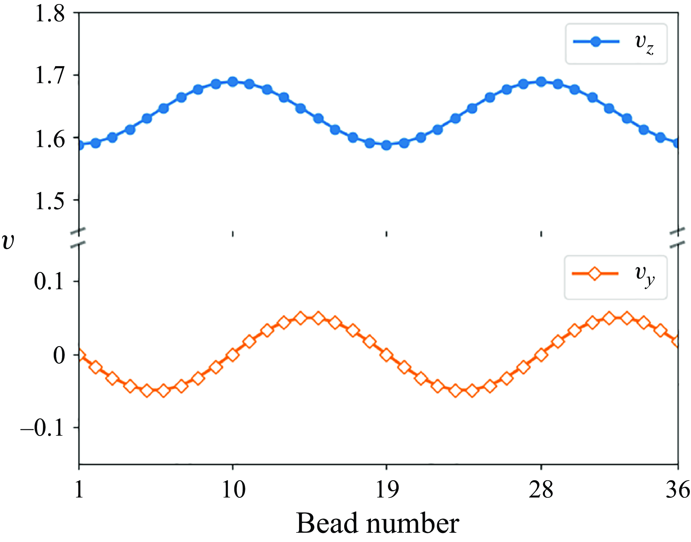
Figure 24. A circular vertical loop in the elastic equilibrium is not stationary. Vertical ( $v_z$
, dots) and horizontal (
$v_z$
, dots) and horizontal ( $v_y$
, diamonds) components of the
$v_y$
, diamonds) components of the $i$
th bead velocity
$i$
th bead velocity $\boldsymbol{v}_{i}^{\parallel }$
vary with the bead number
$\boldsymbol{v}_{i}^{\parallel }$
vary with the bead number $i$
.
$i$
.
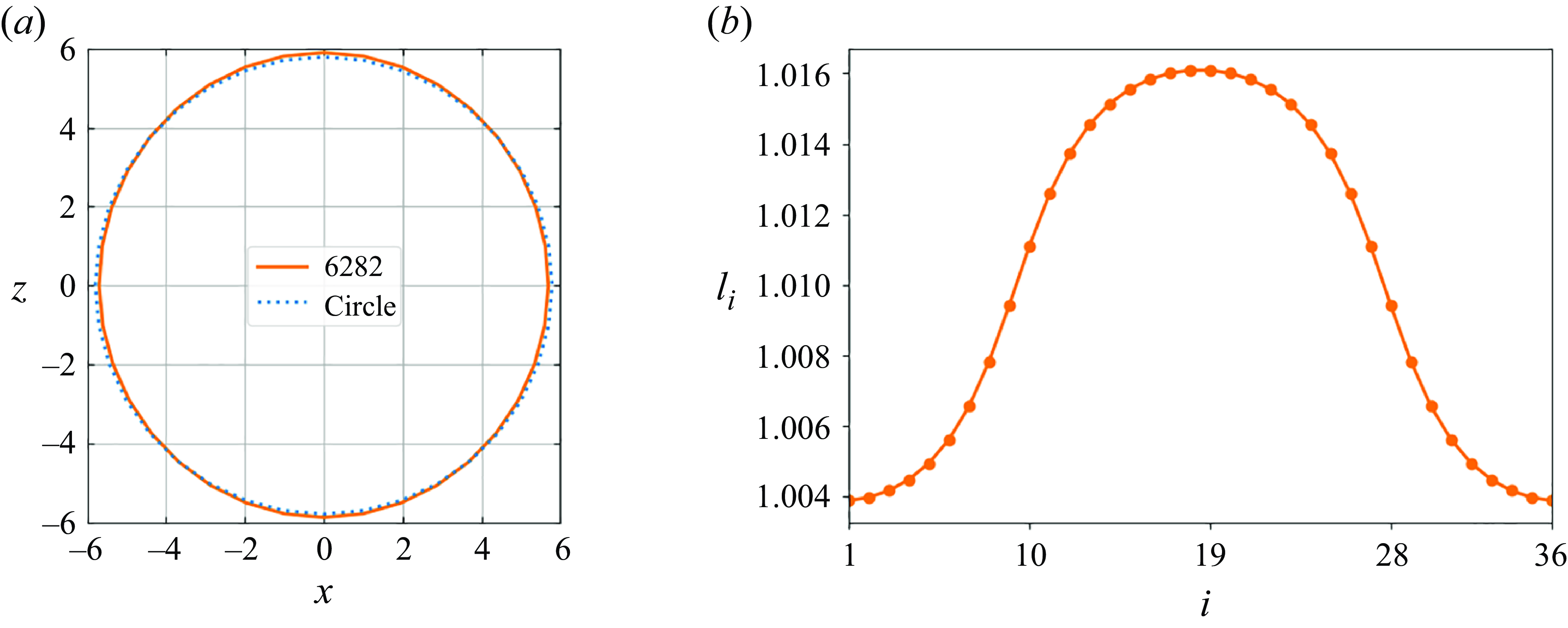
Figure 25. The planar vertical stationary shape of the elastic loop in the attracting vertical mode for $N$
= 36 and
$N$
= 36 and $B$
= 6282 (solid line in (a)) is shown to differ from a circle (dotted line in (a)). The distance between the consecutive beads
$B$
= 6282 (solid line in (a)) is shown to differ from a circle (dotted line in (a)). The distance between the consecutive beads $l_i$
depends on the bead position – it is the smallest at the bottom, and the largest at the top, as visible in (b), with
$l_i$
depends on the bead position – it is the smallest at the bottom, and the largest at the top, as visible in (b), with $l_i=|\boldsymbol{r}_{i+1}-\boldsymbol{r}_{i}|$
for
$l_i=|\boldsymbol{r}_{i+1}-\boldsymbol{r}_{i}|$
for $i=1,\ldots ,N-1$
, and
$i=1,\ldots ,N-1$
, and $l_N=|\boldsymbol{r}_{1}-\boldsymbol{r}_{N}|$
. The distance in the elastic equilibrium equals to 1.01.
$l_N=|\boldsymbol{r}_{1}-\boldsymbol{r}_{N}|$
. The distance in the elastic equilibrium equals to 1.01.
In a certain range of
$B$
, there exists a planar vertical stationary configuration

Then, we show that the stationary planar vertical configuration of the attracting vertical mode is non-circular, and it is not stationary if placed horizontally. The non-circular, vertical shape of the attracting vertical mode, visible in figure 25, was also reported by Gruziel-Słomka et al. (Reference Gruziel-Słomka, Kondratiuk, Szymczak and Ekiel-Jeżewska2019). This shape is not stationary if placed horizontally – velocities of all the beads are not the same, as shown in figure 26. This conclusion can be easily generalised for an inclined loop other than vertical if the gravitational forces are replaced by their projections perpendicular to the loop’s plane. Therefore, the planar configuration observed in the attracting vertical mode is not stationary after tilting by an angle $\theta \ne \pi /2$
.
$\theta \ne \pi /2$
.
A horizontal circle in elastic equilibrium is an unstable stationary configuration
Finally, we argue that the horizontal circular stationary configuration of the loop in the elastic equilibrium is unstable. Indeed, the elastic loop with $B=6283$
, initially horizontal with the shape shown in figure 25, evolves towards a horizontal circle, but then it moves out of the horizontal plane.
$B=6283$
, initially horizontal with the shape shown in figure 25, evolves towards a horizontal circle, but then it moves out of the horizontal plane.
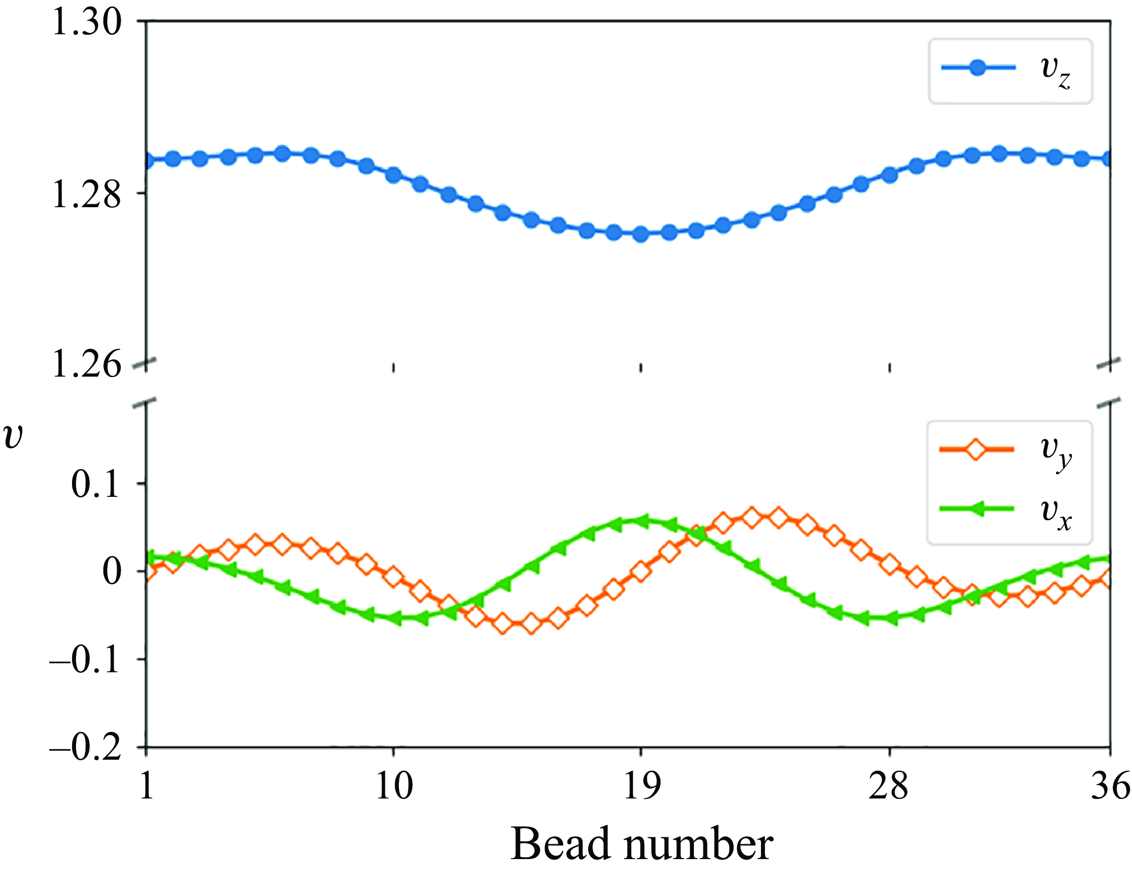
Figure 26. Velocities of the beads for the planar shape from figure 25 placed horizontally ( $z \rightarrow y$
). This configuration is not stationary.
$z \rightarrow y$
). This configuration is not stationary.
Appendix D. Comparison with the dynamics of sedimenting elastic loops in Gruziel-Słomka et al. (Reference Gruziel-Słomka, Kondratiuk, Szymczak and Ekiel-Jeżewska2019)
The results obtained here for the elastic loops made of $N=36$
beads of diameter
$N=36$
beads of diameter $d$
, with their centres at the elastic equilibrium separated by
$d$
, with their centres at the elastic equilibrium separated by $1.01d$
, will be now compared with Gruziel-Słomka et al. (Reference Gruziel-Słomka, Kondratiuk, Szymczak and Ekiel-Jeżewska2019). The same loops are modelled there as an elastic ring made of 60 overlapping beads of the same diameter
$1.01d$
, will be now compared with Gruziel-Słomka et al. (Reference Gruziel-Słomka, Kondratiuk, Szymczak and Ekiel-Jeżewska2019). The same loops are modelled there as an elastic ring made of 60 overlapping beads of the same diameter $d$
, but with their centres at the elastic equilibrium separated by
$d$
, but with their centres at the elastic equilibrium separated by $0.6d$
, which provides approximately the same geometrical aspect ratio. The elasto-gravitation number
$0.6d$
, which provides approximately the same geometrical aspect ratio. The elasto-gravitation number $B$
, used in this work and defined in (2.9), relates in the following way to the stiffness parameter
$B$
, used in this work and defined in (2.9), relates in the following way to the stiffness parameter $\tilde {A}$
used in Gruziel-Słomka et al. (Reference Gruziel-Słomka, Kondratiuk, Szymczak and Ekiel-Jeżewska2019) with the correction in Gruziel-Słomka et al. (Reference Gruziel-Słomka, Kondratiuk, Szymczak and Ekiel-Jeżewska2022),
$\tilde {A}$
used in Gruziel-Słomka et al. (Reference Gruziel-Słomka, Kondratiuk, Szymczak and Ekiel-Jeżewska2019) with the correction in Gruziel-Słomka et al. (Reference Gruziel-Słomka, Kondratiuk, Szymczak and Ekiel-Jeżewska2022),
 \begin{equation} B \approx 1.5 \cdot 10^4 /{\tilde {A}}. \end{equation}
The above comparison is based on assuming (Bukowicki & Ekiel-Jeżewska Reference Bukowicki and Ekiel-Jeżewska2018) that the loop from Gruziel-Słomka et al. (Reference Gruziel-Słomka, Kondratiuk, Szymczak and Ekiel-Jeżewska2019, Reference Gruziel-Słomka, Kondratiuk, Szymczak and Ekiel-Jeżewska2022) has the same bending energy,
 \begin{equation} U^{B} = \sum _{j=1}^{60} \frac {A^{*}}{1.2d} \beta '^2_{j}, \end{equation}
as in (2.2) the loop with $N=36$
considered here. In (D2),
$N=36$
considered here. In (D2), $A^*$
from Gruziel-Słomka et al. (Reference Gruziel-Słomka, Kondratiuk, Szymczak and Ekiel-Jeżewska2019) is the same bending stiffness as
$A^*$
from Gruziel-Słomka et al. (Reference Gruziel-Słomka, Kondratiuk, Szymczak and Ekiel-Jeżewska2019) is the same bending stiffness as $A$
used here.
$A$
used here.
In Gruziel-Słomka et al. (Reference Gruziel-Słomka, Kondratiuk, Szymczak and Ekiel-Jeżewska2019), hydrodynamic interactions between the beads were described by the Rotne–Prager translational–translational mobility matrix (Rotne & Prager Reference Rotne and Prager1969; Yamakawa Reference Yamakawa1970; Zuk et al. Reference Zuk, Wajnryb, Mizerski and Szymczak2014, Reference Zuk, Cichocki and Szymczak2017, Reference Zuk, Cichocki and Szymczak2018). This approach does not include the lubrication forces caused by the relative motion of close bead surfaces (in contrast to our method). To compensate, in Gruziel-Słomka et al. (Reference Gruziel-Słomka, Kondratiuk, Szymczak and Ekiel-Jeżewska2019), the consecutive beads overlap, and small short-distance repelling forces are added. This approach allows for monitoring the motion of very elastic loops, such as the bent figure eight or toroidal attracting modes. Such compact modes cannot be studied by our present numerical approach. Another advantage of the Rotne–Prager method is that the simple analytical form of the mobility coefficients allows for fast computations. The benefit of the multipole expansion corrected for lubrication (used here) is a controlled high precision.
The attracting dynamical modes (vertical, tilted, frozen rotating, swinging, flapping) observed in the Rotne–Prager approximation (Gruziel-Słomka et al. Reference Gruziel-Słomka, Kondratiuk, Szymczak and Ekiel-Jeżewska2019) have also been found here. The transition between vertical and tilted modes takes place at approximately the same value of $B$
. The coexistence of different modes, found in Gruziel-Słomka et al. (Reference Gruziel-Słomka, Kondratiuk, Szymczak and Ekiel-Jeżewska2019), is confirmed here. However, in the present work, two new modes and some differences in the phase diagram are reported. Moreover, here all the modes are described quantitatively, including the characteristic time scales, velocities and transitions between the modes.
$B$
. The coexistence of different modes, found in Gruziel-Słomka et al. (Reference Gruziel-Słomka, Kondratiuk, Szymczak and Ekiel-Jeżewska2019), is confirmed here. However, in the present work, two new modes and some differences in the phase diagram are reported. Moreover, here all the modes are described quantitatively, including the characteristic time scales, velocities and transitions between the modes.


 Open access