Flow-induced oscillations of a clamped flexible ring

Abstract

The flow-induced oscillations of a clamped flexible ring in a uniform flow were explored using the penalty immersed boundary method. Both inverted and conventional ring configurations were examined, with systematic analysis focused on the effects of bending rigidity and eccentricity. Four distinct oscillation modes were identified across parameter variations: flapping (F), deflected oscillation (DO), transverse oscillation (TO) and equilibrium (E) modes. Each mode exhibited a 2S wake pattern. The inverted ring sustained the DO mode under low bending rigidity with a deflected shape, transitioning to the TO mode at higher bending rigidity. In the TO mode, a lock-in phenomenon emerged, enabling the inverted ring to achieve a high power coefficient due to a simultaneous rise in both oscillation amplitude and frequency. By contrast, the conventional ring exhibited the F mode at low bending rigidity and transitioned to the E mode as rigidity increased, although its power coefficient remained lower because of reduced critical bending rigidity. For the inverted ring, low eccentricity enhanced oscillation intensity but limited the operational range of the TO mode. In contrast, for the conventional ring, reducing eccentricity led to an increase in oscillation amplitude. Among the investigated configurations, the inverted-clamped ring achieved the highest energy-harvesting efficiency, surpassing those of the conventional clamped ring and a buckled filament.

1. Introduction

The increasing reliance on fossil fuels has led to significant environmental pollution and climate change, prompting a shift toward clean energy sources. One promising approach involves harnessing flow-induced oscillations in flexible structures to convert flow energy into electricity using piezoelectric materials. These devices have diverse applications, including self-powered sensor networks, structural health monitoring for bridges and offshore platforms and supplementary energy sources for urban infrastructure. Additionally, they offer potential for capturing wind and water flow energy in remote or underwater environments where conventional power sources are impractical (Wang et al. 2020; Sezer & Koç 2021). Among these innovative designs, a flexible ring, which is capable of storing elastic energy in its initial state, shows substantial potential for energy harvesting. Thus, understanding the flow-induced oscillations of flexible rings is essential for advancing flexible energy-harvesting technologies.

Figure 1. Two energy harvesters based on flow-induced vibration: (a) a one-edge-clamped flag and (b) a two-edge-clamped flag.

Flexible energy harvesters are commonly made from piezoelectric materials. Although environmental factors can influence their properties, recent advancements have enhanced their durability and performance, highlighting their significant potential for energy harvesting. Traditional flexible energy harvesters that rely on flow-induced vibrations are generally categorised based on their edge conditions into two types: conventional flags and inverted flags (figure 1 a). The energy-harvesting performance of these systems is closely linked to factors such as critical bending rigidity, oscillation frequency and filament deflection during motion (Doaré & Michelin 2011; Michelin & Doaré 2013; Shoele & Mittal 2016). A conventional flag, characterised by a clamped leading edge and a free trailing edge, exhibits different oscillation modes – stretched straight, limit-cycle flapping and chaotic flapping – depending on its Reynolds number (Re), mass ratio, filament length and bending rigidity (Zhang et al. 2000; Zhu & Peskin 2003; Shelley, Vandenberghe & Zhang 2005; Alben & Shelley 2008; Michelin, Llewellyn Smith & Glover 2008; Banerjee, Connell & Yue 2015; Cisonni et al. 2017). The flapping motion of a conventional flag is considered flutter caused by structural instability, resulting in high-frequency, low-amplitude oscillations (Connell & Yue 2007; Eloy et al. 2008; Uddin, Huang & Sung 2015). However, the low critical bending rigidity of conventional flags limits their energy-harvesting performance (Michelin & Doaré 2013). By contrast, the inverted flag, which has a clamped trailing edge and a free leading edge, was introduced by Kim et al. (2013) to address this limitation by increasing the critical bending rigidity and enhancing the oscillation amplitude. Inverted flags display three distinct modes – straight, flapping and deflected – as the bending rigidity, flow velocity and filament length vary (Gurugubelli & Jaiman 2015; Tang, Liu & Lu 2015; Sader et al. 2016; Orrego et al. 2017; Yu, Liu & Chen 2017; Tavallaeinejad et al. 2020a , b ). The inverted flag achieves greater deflection and higher critical bending rigidity than the conventional flag, thus offering superior energy-harvesting performance (Ryu et al. 2015; Shoele & Mittal 2016). Despite these advantages, both conventional and inverted flags share a common limitation: one end is clamped while the other remains free. This configuration restricts the deflection of the flags, limiting their potential for energy harvesting.

To address limitations in flow energy harvesting, researchers used buckled filaments clamped at both ends (figure 1 b), storing substantial elastic energy in their initial shape (Chen, Liu & Sung 2024). Kim et al. (2020) examined the snap-through oscillation (STO) of such filaments for energy-harvesting applications. Mao, Liu & Sung (2023) applied the immersed boundary (IB) method to examine how filament length, bending rigidity and Reynolds number influence the snap-through dynamics, identifying three modes: STO, streamwise oscillation and equilibrium. The STO mode in buckled filaments shows substantial deformation but requires high external energy for initiation, leading to low critical bending rigidity (Kim et al. 2021). Moreover, the STO mode’s oscillation frequency is lower than that of conventional and inverted flags, limiting the energy-harvesting capacity of buckled filaments. To enhance critical bending rigidity and increase oscillation frequency, recent studies (Chen et al. 2023, 2024) investigated the effects of edge conditions and walls on STO performance. Although these modifications adjust the initiation conditions, they still yield insufficient critical bending rigidity and oscillation frequency, constraining the utility of buckled filaments for effective energy harvesting. To address these limitations, we propose using a transversely clamped filament, where the clamped edges are rotated 90° to align perpendicular to the flow direction (Chen, Liu & Sung 2025). This configuration creates two types of transversely clamped buckled filaments – inverted and conventional – depending on the orientation. When the bending rigidity, filament length and Reynolds number are varied, several oscillation modes emerge: conventional transverse oscillation (TO), deflected oscillation, inverted TO and equilibrium. The TO mode, in particular, is driven by periodic vortex shedding from the filament’s bluff body, making it easier to initiate. The TO mode is also associated with a higher critical bending rigidity and synchronises with vortex shedding, resulting in a higher oscillation frequency than the STO mode, thereby improving energy-harvesting efficiency.

Although the larger deflection and higher frequency of the TO mode enhance the energy-harvesting potential compared with that of single-end-clamped filaments, the fixed distance between the clamped edges limits the motion of transversely clamped filaments. This constraint reduces the oscillation amplitude, thereby limiting overall energy generation in the TO mode. To overcome this challenge, we propose a flexible ring configuration in which the clamped edges of the buckled filament are positioned closer together. This design eliminates the fixed-edge constraint, enabling greater oscillation amplitude and improved energy-harvesting performance. In addition, the ring shape, as a classic bluff body, inherently generates vortices that induce TOs, similar to vortex-induced vibrations observed in elastically mounted cylinders (Bearman 1984; Williamson & Govardhan 2004; Prasanth & Mittal 2008; Navrose & Mittal 2016; Fan et al. 2019).

Previous research has examined flow-induced oscillations in flexible rings with one side pinned (Jung et al. 2006; Shoele & Zhu 2010; Kim et al. 2012), whereas studies on clamped flexible rings remain limited. Understanding the fluid dynamics governing the oscillations of clamped flexible rings is crucial for advancing flexible energy-harvesting technology. Bending rigidity is a key factor influencing energy-harvesting efficiency. However, the experimental manipulation of bending rigidity is often constrained by material limitations. As a result, numerical approaches, such as the IB method, offer a practical and effective alternative for analysing these complex fluid–structure interactions (Huang, Shin & Sung 2007; Huang & Sung 2010; Huang, Chang & Sung 2011; Ryu et al. 2015).

The objective of the present study is to explore the flow-induced oscillations in clamped flexible rings using the penalty IB method. Two configurations – conventional and inverted rings – are analysed to assess the effects of bending rigidity ( $\gamma$ ) and ring eccentricity ( $\epsilon$ ) on mode transitions and energy-harvesting performance. The motion of the rings and their corresponding wake patterns are analysed across different modes, with the lock-in phenomenon identified through oscillation amplitude and frequency analysis. We compare the behaviour and underlying mechanisms of the flexible ring with other flexible energy harvesters. Additionally, we assess the contributions of each component to energy harvesting in both configurations and derive an estimate of the power coefficient using dimensional analysis. Lastly, we compare the energy-harvesting performance of clamped rings with those of streamwise and transversely buckled filaments.

2. Computational model

2.1. Problem formulation

Clamped flexible rings can be classified into two configurations on the basis of their clamping orientation: conventional and inverted. Figure 2 illustrates these configurations, where $L$ denotes a ring’s length and $a$ and $b$ represent its major and minor axes, respectively. The ring’s eccentricity is defined by $\epsilon$ . Blue boxes at both ends indicate clamped boundary conditions. Fluid motion is analysed in a fixed Eulerian coordinate system, with the domain spanning $-10L_{0}\leq x\leq 22L_{0}$ in the streamwise direction and $-8L_{0}\leq y\leq 8L_{0}$ in the transverse direction. Here, $L_{0}$ represents the equivalent diameter of an elliptic ring, which corresponds to the diameter of a circular ring when $\epsilon = 1$ . Dirichlet boundary conditions ( $u=U_{0}$ , $v=0$ ) are applied at the inlet, top and bottom boundaries, whereas a Neumann boundary condition ( $\partial \boldsymbol{u}/\partial x=0$ ) is set at the outlet (Huang & Sung 2007). The filament’s motion is described in a moving curvilinear coordinate system, where $s$ denotes the filament’s arc length.

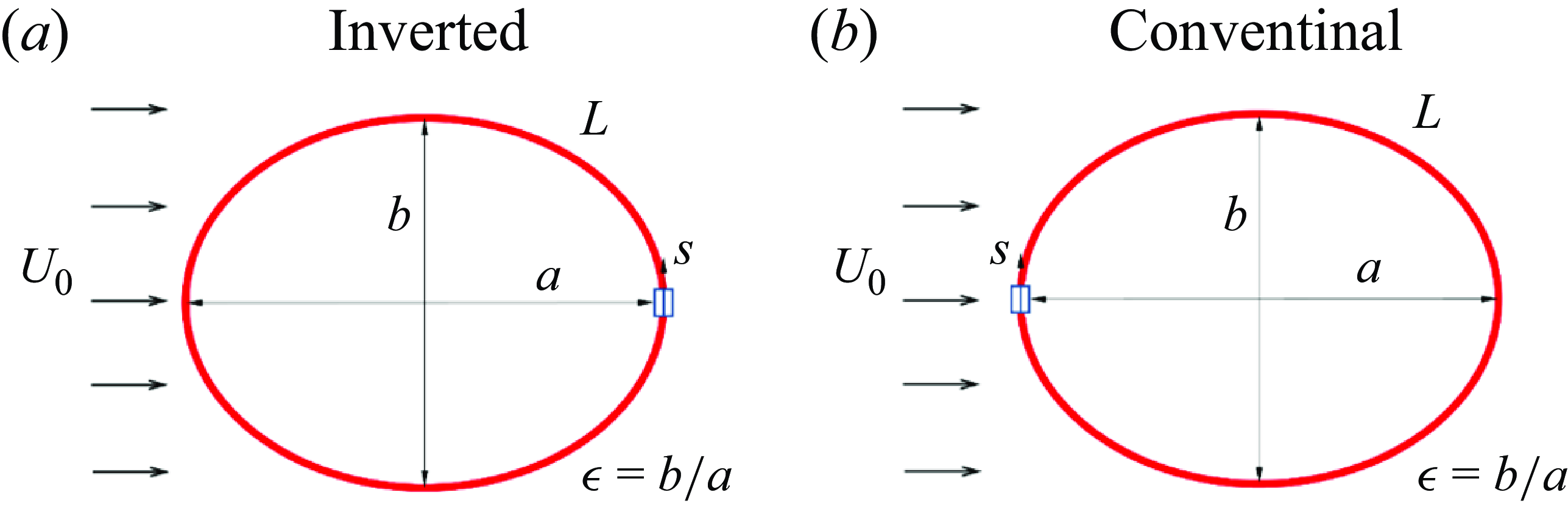
Figure 2. Schematics of ( $a$ ) inverted and ( $b$ ) conventional clamped flexible rings in a uniform flow.

The fluid motion is governed by the Navier–Stokes equations and the continuity equation, which are expressed in their non-dimensional forms as

(2.1) \begin{equation}\frac{\partial \boldsymbol{u}}{\partial t}+\boldsymbol{u}\cdot \nabla \boldsymbol{u}=-\nabla p+\frac{1}{Re}\nabla ^{2}\boldsymbol{u}+\boldsymbol{f},\end{equation}

(2.2) \begin{equation}\nabla \cdot \boldsymbol{u}=0,\end{equation}

where $\boldsymbol{u}=(u$ , $v)$ represents the fluid velocity vector, $p$ is the pressure and $\boldsymbol{f}=(f_{x}$ , $f_{y})$ denotes the momentum forcing used to enforce the no-slip boundary condition along the IB. The Reynolds number is defined as $Re=\rho _{0}U_{0}D/\mu$ , where $\rho _{0}$ and $\mu$ are the fluid density and the dynamic viscosity, respectively. Equations (2.1) and (2.2) are non-dimensionalised using the following characteristic scales: $L_{0}$ for length, $U_{0}$ for velocity, $L_{0}/U_{0}$ for time, $\rho _{0}{U_{0}}^{2}$ for pressure and $\rho _{0}{U_{0}}^{2}/L_{0}$ for the momentum forcing $\boldsymbol{f}$ . For simplicity, the dimensionless variables are expressed in the same form as their dimensional counterparts.

The motion of the flexible structure is governed by the nonlinear structural equation and the inextensibility condition, which are expressed in their non-dimensional forms as

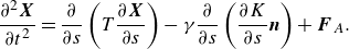
(2.3) \begin{equation}\frac{\partial ^{2}\boldsymbol{X}}{\partial t^{2}}=\frac{\partial }{\partial s}\left(T\frac{\partial \boldsymbol{X}}{\partial s}\right)-\gamma \frac{\partial }{\partial s}\left(\frac{\partial K}{\partial s}\boldsymbol{n}\right)-\boldsymbol{F}_{{f}},\end{equation}

(2.4) \begin{equation}\frac{\partial \boldsymbol{X}}{\partial s}\cdot \frac{\partial \boldsymbol{X}}{\partial s}=1,\end{equation}

where $\boldsymbol{X}=(X(s,t),Y(s,t))$ denotes the displacement vector of the filament, $s$ is the arclength, $T$ and $\gamma$ represent the tension coefficient and bending rigidity along the filament, respectively, $K$ is the curvature of the filament, $\boldsymbol{n}$ denotes the normal direction and $\boldsymbol{F}_{{f}}$ represents the Lagrangian momentum forcing exerted by the surrounding fluid on the filament. These equations are non-dimensionalised using the following characteristic scales: $D$ for length, $L_{0}/U_{0}$ for time, $\rho _{1}U_{0}^{2}$ for the tension coefficient $T$ $\rho _{1}U_{0}^{2}L_{0}^{2}$ for the bending rigidity $\gamma$ and $\rho _{1}U_{0}^{2}/L_{0}$ for the Lagrangian forcing $\boldsymbol{F}_{{f}}$ , where $\rho _{1}$ denotes the density difference between the filament and the surrounding fluid. Given that the filament’s cross-sectional length is negligible, $\rho _{1}$ is considered the density of the filament. The elastic force of the filament is given by $\boldsymbol{F}_{{s}}=({\partial }/{\partial s})(T ({\partial \boldsymbol{X}}/{\partial s}))-\gamma ({\partial }/{\partial s})(({\partial K}/{\partial s})\boldsymbol{n})$ . In the present study, the value of $\gamma$ is constant during filament motion, whereas $T$ is a function of both $s$ and $t$ , determined by the inextensibility condition. A Poisson equation is constructed to solve the value of $T$ (Huang et al. 2007). Clamped boundary conditions are applied at the two fixed edges of the filament, which are

(2.5) \begin{equation}{\partial \boldsymbol{X}}/{\partial s}= (0,1)\quad {\rm at}\quad s=0,L.\end{equation}

The penalty IB method is used to calculate the interaction between the filament and the fluid. In this method, the IB is divided into a `massive boundary’ and a `massless boundary,’ which are connected by a stiff spring to simulate the interaction. The Lagrangian force $\boldsymbol{F}_{{f}}$ exerted by the fluid on the filament is computed using the equation (Goldstein, Handler & Sirovich 1993)

(2.6) \begin{equation}\boldsymbol{F}_{{f}}=\alpha \int _{0}^{t}\left(\boldsymbol{U}_{{ib}}-\boldsymbol{U}\right)\mathrm{d}t^{\prime}+\beta \left(\boldsymbol{U}_{{ib}}-\boldsymbol{U}\right),\end{equation}

where $\alpha = -3\times 10^{6}$ and $\beta = -$ 100 are large negative constants chosen to enforce the no-slip boundary condition (Huang et al. 2007; Shin, Huang & Sung 2008). Here, $\boldsymbol{U}_{{ib}}$ represents the velocity of the massless boundary, as obtained by interpolation at the IB, and $\boldsymbol{U}$ is the velocity of the massive boundary obtained by $\boldsymbol{U}=\mathrm{d}\boldsymbol{X}/\mathrm{d}t$ . The transformation between Eulerian (fluid) and Lagrangian (filament) variables is achieved using the Dirac delta function. The parameters $\boldsymbol{U}_{{ib}}$ and $\boldsymbol{f}$ are calculated using the equations

(2.7) \begin{equation}\boldsymbol{U}_{{ib}}\left(s,t\right)=\int _{\Omega }\boldsymbol{u}\left(x,t\right) \delta \left(\boldsymbol{X}\left(s,t\right)-x\right)\mathrm{d}x,\end{equation}

(2.8) \begin{equation}\boldsymbol{f}(x,t)=\rho \int _{{\Gamma} }\boldsymbol{F}_{{f}}(s,t) \delta (x-\boldsymbol{X}(s, t))\mathrm{ds},\end{equation}

where the density ratio ( $\rho$ ) is derived from the non-dimensionalisation process ( $\rho =\rho _{1}/\rho _{0}D=1$ ). In this context, $\rho _{1}$ refers to the line density, whereas $\rho _{0}$ represents the area density.

To address the issue of volume conservation in simulations involving incompressible fluids enclosed by a flexible ring, we used a penalty IB method incorporating fluid compressibility (Peng, Asaro & Zhu 2010; Kim et al. 2012). This method compensates for the volume leakage caused by the smoothed Dirac delta function in traditional IB methods. The compressibility of the fluid is defined as

(2.9) \begin{equation}\beta =-\frac{1}{V}\frac{\partial V}{\partial p},\end{equation}

where $V$ is the volume enclosed by the ring and $p$ represents the pressure. On the basis of this relationship, the pressure difference can be expressed as

(2.10) \begin{equation}\Delta p=\frac{1}{\beta }\left(1-\frac{V}{V_{0}}\right),\end{equation}

where $V_{0}$ represents the initial volume. To enhance volume conservation, an integral term, inspired by proportional-integral control, is added to mitigate steady-state error, yielding an updated pressure difference expression (Kim et al. 2012)

(2.11) \begin{equation}\Delta p=\frac{1}{\beta }\left(1-\frac{V}{V_{0}}\right)+\int _{0}^{t}\frac{1}{\beta }\left(1-\frac{V}{V_{0}}\right)\mathrm{d}t^{\prime}.\end{equation}

The penalty force ensuring volume conservation is then derived as

(2.12) \begin{equation}F_{{A}}\left(s\right)=\Delta p\boldsymbol{e}_{n},\end{equation}

where $\boldsymbol{e}_{n}$ is the local outward normal vector of the ring. Consequently, the structural equation incorporating the volume conservation force is formulated as

(2.13) \begin{equation}\frac{\partial ^{2}\boldsymbol{X}}{\partial t^{2}}=\frac{\partial }{\partial s}\left(T\frac{\partial \boldsymbol{X}}{\partial s}\right)-\gamma \frac{\partial }{\partial s}\left(\frac{\partial K}{\partial s}\boldsymbol{n}\right)+\boldsymbol{F}_{{A}}.\end{equation}

To evaluate the electrical energy generated by the flexible ring, the piezoelectric–structure coupling effect is incorporated. The flexible ring surface is assumed to be fully covered with infinitesimal piezoelectric patches, each with a segmentation length substantially smaller than L, connected to external circuits. These patches convert strain energy into electrical energy as the filament deflects. The concurrent application of an electric voltage to the electrodes induces additional internal torque on both the piezoelectric patches and the filament (Doaré & Michelin 2011). The local electrical state of each patch is described by the electric voltage between the positive electrodes, denoted as $V(s,t)$ , and the charge transfer $Q(s,t)$ along the filament axis, both of which are continuous functions of $s$ and $t$ (Michelin & Doaré 2013). The piezoelectric coupling effect is governed by the following equations:

(2.14) \begin{equation}Q\left(s,t\right)=cV+\chi K,\end{equation}

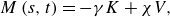(2.15) \begin{equation}M\left(s,t\right)=-\gamma K+\chi V,\end{equation}

where $M(s,t)$ represents the torque of the filament and $c$ and $\chi$ are the lineic capacitance and piezoelectric coupling coefficient, respectively, which are related to the material and geometric properties of the patch pair (Doaré & Michelin 2011). The positive electrodes are connected to a purely resistive circuit with lineic conductivity, as described by the following equation:

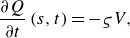(2.16) \begin{equation}\frac{\partial Q}{\partial t}\left(s,t\right)=-\varsigma V,\end{equation}

where $\varsigma$ represents the linear conductivity coefficient between the piezoelectric patches on the upper and lower surfaces of the filament. When the piezoelectric effect is taken into account, the equivalent bending rigidity can be expressed as

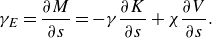(2.17) \begin{equation}\gamma _{{E}}=\frac{\partial M}{\partial s}=-\gamma \frac{\partial K}{\partial s}+\chi \frac{\partial V}{\partial s}.\end{equation}

By combining equations (2.14)−(2.17), we can express the nonlinear structure equation incorporating the piezoelectric effect, the inextensible condition and the electrical equation as follows:

(2.18) \begin{equation}\frac{\partial ^{2}\boldsymbol{X}}{\partial t^{2}}=\frac{\partial }{\partial s}\left(T\frac{\partial \boldsymbol{X}}{\partial s}\right)-\gamma \frac{\partial }{\partial s}\left(\frac{\partial K}{\partial s}\boldsymbol{n}\right)+\alpha _{{e}}\sqrt{\gamma }\frac{\partial }{\partial s}\left(\frac{\partial V}{\partial s}\boldsymbol{n}\right)-\boldsymbol{F}_{{f}}+\boldsymbol{F}_{{A}},\end{equation}

(2.19) \begin{equation}\frac{\partial \boldsymbol{X}}{\partial s}\cdot \frac{\partial \boldsymbol{X}}{\partial s}=1,\end{equation}

(2.20) \begin{equation}\beta _{{e}}\frac{\partial V}{\partial t}=-V-\alpha _{{e}}\beta _{{e}}\sqrt{\gamma }\frac{\partial K}{\partial t},\end{equation}

where $\alpha _{{e}}=\chi /\sqrt{c\gamma _{L}}$ and $\beta _{{e}}=cU/\varsigma L$ represent the coupling coefficient and the tuning coefficient of the electrical system, respectively (Shoele & Mittal 2016). Here, $\gamma _{{L}}$ denotes the dimensional bending rigidity of the filament. The voltage and charge density are non-dimensionalised by $U\sqrt{\rho L/c}$ and $U\sqrt{\rho Lc}$ , respectively. In the present study, $\alpha _{{e}}$ and $\beta _{{e}}$ are held constant at values of 0.1, ensuring that they do not affect the overall filament motion.

The energy-harvesting performance can be evaluated by examining both the elastic strain energy $E_{{s}}$ and the power coefficient c _p . Here, $E_{{s}}$ represents the strain energy generated by the filament’s deformation during motion. It is defined as

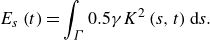(2.21) \begin{equation}E_{{s}}\left(t\right)=\int _{\Gamma }0.5 \gamma K^{2}\left(s,t\right)\mathrm{d}s.\end{equation}

In addition, the harvested energy, which corresponds to the instantaneous power dissipated in the piezoelectric patches (Michelin & Doaré 2013; Shoele & Mittal 2016), can be quantified using the power coefficient, defined as

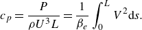(2.22) \begin{equation}c_{{p}}=\frac{P}{\rho U^{3}L}=\frac{1}{\beta _{{e}}}\int _{0}^{L}V^{2}\mathrm{d}s.\end{equation}

The fractional step method on a staggered Cartesian grid is used to solve the Navier–Stokes equations (Kim, Baek & Sung 2002). A direct numerical method developed by Huang et al. (2007) is used to calculate the filament motion. Details of the discretisation of the governing equations and numerical method can be found in the works of (Kim et al. 1992, 2002). We validated the accuracy of the solver in capturing the dynamics of the flexible ring in our previous work (Kim et al. 2012: Lee, Sung & Zaki 2017).

2.2. Validation

Table 1 presents the results of the domain test for the conventional clamped ring with $\epsilon = 0.6$ , $\gamma =$ 0.01 and $Re=$ 100. These results include the averaged drag coefficient $\overline{C}_{{D}}$ , oscillation amplitude $A_{y}$ and the Strouhal number $St$ ( $=f_{v}D/U_{0}$ ), along with the corresponding relative error $\varepsilon$ . Here, $f_{v}$ represents the vortex shedding frequency from the ring. The simulation does not converge for the $16\times 16$ domain. The results for the $32\times 16$ domain are consistent with those for the $32\times 24$ and $64\times 16$ domains. Therefore, a domain size of $32\times 16$ was selected because it allows for simulation over a greater number of time steps, thereby enhancing the accuracy of the results. To assess the effect of grid resolution and time step on the simulation outcomes, we conducted convergence studies for various grid resolutions and time steps. Figure 3 shows the time evolution of the transverse displacement at the midpoint of the ring. The results obtained for $\Delta x=1/64$ and $\Delta t=4\times 10^{-4}$ align well with those for $\Delta x=1/128$ and $\Delta t=2\times 10^{-4}$ . Consequently, a grid resolution of $1/64$ and a time step of $4\times 10^{-4}$ were chosen to ensure high accuracy in the simulation. The maximum Courant number was approximately 0.04 in the simulation. The grid was uniform in the $x$ -direction but stretched in the $y$ -direction. Specifically, within the range $-Y/4\leq y\leq Y/4$ , the grid size was $\Delta y=\Delta x$ . Outside this range, the grid size was adjusted to $\Delta y=2\Delta x$ . The grid resolution for the ring was chosen to match that of the surrounding fluid domain for consistency.

Table 1. Domain test, including the averaged drag coefficient $\overline{C}_{{D}}$ , oscillation amplitude of $A_{y}$ , the Strouhal number $St$ and the relative errors $e$ to $32\times 24$ (domain height test in part I) and $64\times 16$ (domain length test in part II) in the conventional configuration ( $L/D=3$ , $\gamma =0.01$ , $Re=100$ ).

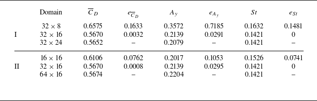
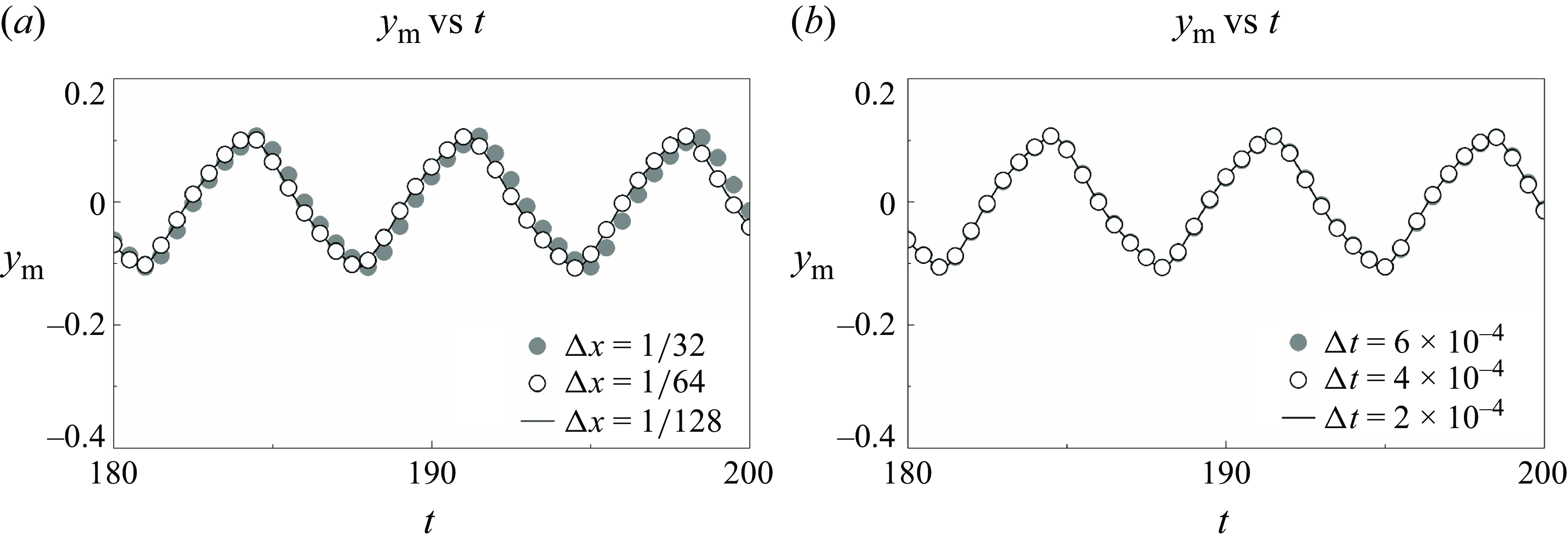
Figure 3. Time evolution of the transverse displacement of the midpoint of the ring ( $y_{{m}}$ ) for different (a) grid sizes and (b) time steps.

To validate our simulation framework, we conducted experiments in a small open suction wind tunnel with wind speeds ranging from 10 to 55 m s^–1. An event camera was used to capture the instantaneous shapes of the flexible ring. The ring was fabricated from polyethylene terephthalate (PET) film with a thickness of 0.05 mm, a Young’s modulus of 4 GPa, a Poisson’s ratio of 0.4 and a density of 1.3 × 10³ kg m^–3. Details of the experimental setup are provided in the work of Lyu, Cai & Liu (2024). Obtaining high-quality Particle Image Velocimetry measurements was challenging due to the PET film’s tendency to reflect and scatter the laser sheet, as well as optical occlusions resulting from the ring’s continuously varying curvature. Instead, we focused on examining the influence of non-dimensional bending rigidity on the oscillation amplitude ( $A_{y}$ ), providing valuable insights into the ring’s dynamic behaviour under varying aerodynamic conditions (Chen et al. 2024, 2025). Although varying the wind speed to modify $\gamma$ makes it challenging to maintain a constant $Re$ , our experiments captured three distinct oscillation modes that match the predictions from our numerical simulations (figure 4). Moreover, our investigation into the effect of the ring’s aspect ratio ( $W/L_{0}$ , where $W$ is the ring’s spanwise width and $L_{0}$ is the equivalent diameter) showed that as $W/L_{0}$ increases, $A_{y}$ converges to a constant value, indicating that three-dimensional effects become negligible (Banerjee et al. 2015; Gurugubelli & Jaiman 2019). Overall, experimental studies are limited by the difficulty of altering the parameters of filament materials, which constrains the scope of research. In contrast, simulations offer greater flexibility, enabling the exploration of a broader range of parameters and the examination of additional phenomena.

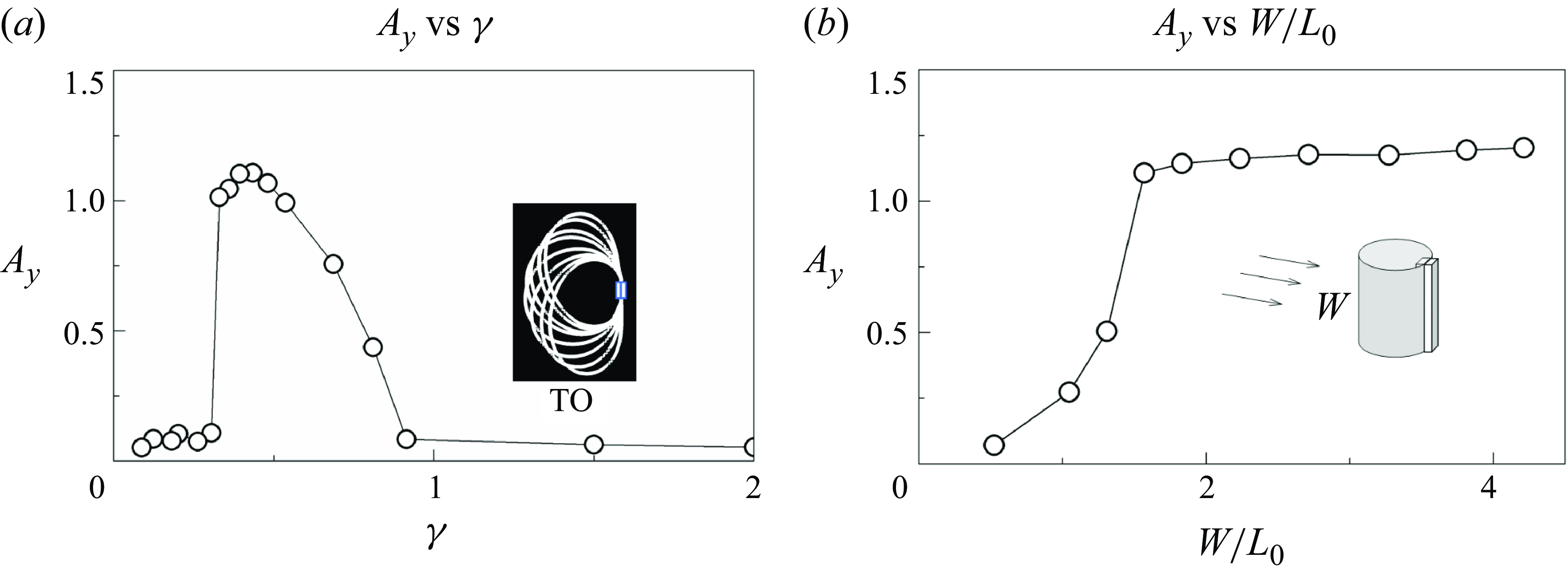
Figure 4. Oscillation amplitude for an inverted ring as a function of (a) $\gamma$ and (b) $W/L_{0}$ .

3. Results and discussion

3.1. Modes of ring motion

We examined the motion and wake patterns of both conventional and inverted flexible rings under different dynamic modes. As shown in figure 5, the flapping (F) mode, deflected oscillation (DO) mode, and TO mode were identified as $\gamma$ was varied, with $\epsilon = 0.65$ kept constant. Experimental observations are included in each inset for qualitative comparison. The F mode, resembling the motion of a conventional flag, is characterised by low-amplitude, high-frequency oscillations and occurs in the conventional configuration. By contrast, the inverted configuration exhibits either DO or TO, depending on the conditions. In the DO mode, the ring deflects to one side and undergoes low-amplitude oscillations, similar to an inverted flag. As $\gamma$ increases, the ring transitions to the TO mode, characterised by large-amplitude oscillations perpendicular to the flow direction. The experiments were conducted in a wind tunnel, where the three modes were identified as the wind speed was varied under comparable bending rigidity. Despite differences between the simulation and experimental conditions, the qualitatively similar results confirm the existence of these modes. Experimental studies are constrained by the difficulty of altering filament material parameters, limiting the scope of research. By contrast, simulations enable broader parameter exploration and the study of additional phenomena in both inverted and conventional flexible rings.

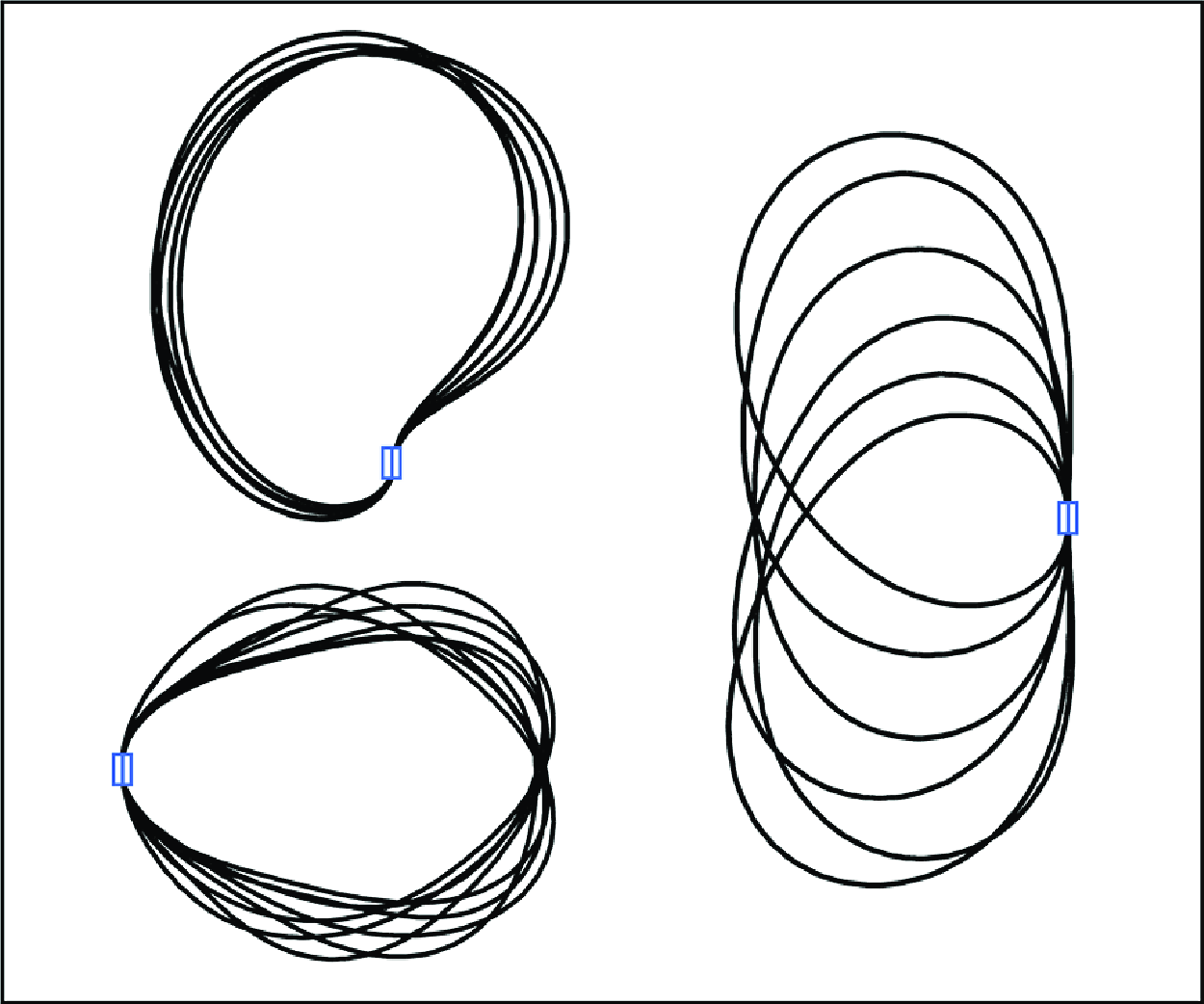
Figure 5. Superposition of the instantaneous shapes of the flexible ring for different oscillation modes: (a) F mode at $\gamma =$ 0.01, (b) DO mode at $\gamma =$ 0.02 and (c) TO mode at $\gamma =$ 0.5, with $\epsilon = 0.65$ . The white line in each inset represents the experimentally observed mode.

To illustrate the distribution of modes for both inverted and conventional flexible rings as $\gamma$ and $\epsilon$ were varied, mode diagrams are presented in figure 6. All simulations in the present study are run for at least 80 oscillation cycles to ensure that the motion has fully converged. For the inverted flexible ring, three distinct modes emerge depending on $\gamma$ and $\epsilon$ . At low bending rigidity and in the transition zone between the TO and equilibrium (E) modes, the DO mode dominates. This mode is characterised by motion confined to one side of the $y$ -axis, resembling the DO mode of the inverted flag. Unlike the symmetric up-and-down flapping observed in the conventional ring, the DO mode occurs asymmetrically on one side, either above or below the $x$ -axis, depending on the initial excitation. As $\gamma$ increases to a level where the flexible ring can resist the fluid forces, the ring transitions into the TO mode, where it exhibits symmetric oscillation along the $y$ -axis. Notably, the TO mode is more likely to occur at higher $\epsilon$ values and is absent at lower $\epsilon$ values (i.e. $\epsilon = 0.2$ ), possibly because of the flatter shape of the ring under low $\epsilon$ , which causes it to deflect to one side rather than oscillate in the TO motion. When $\gamma$ becomes sufficiently high, the ring’s motion diminishes, eventually leading to the E mode. By contrast, the conventional ring only exhibits two modes: the F mode at low $\gamma$ and the E mode as $\gamma$ increases beyond the critical bending rigidity.

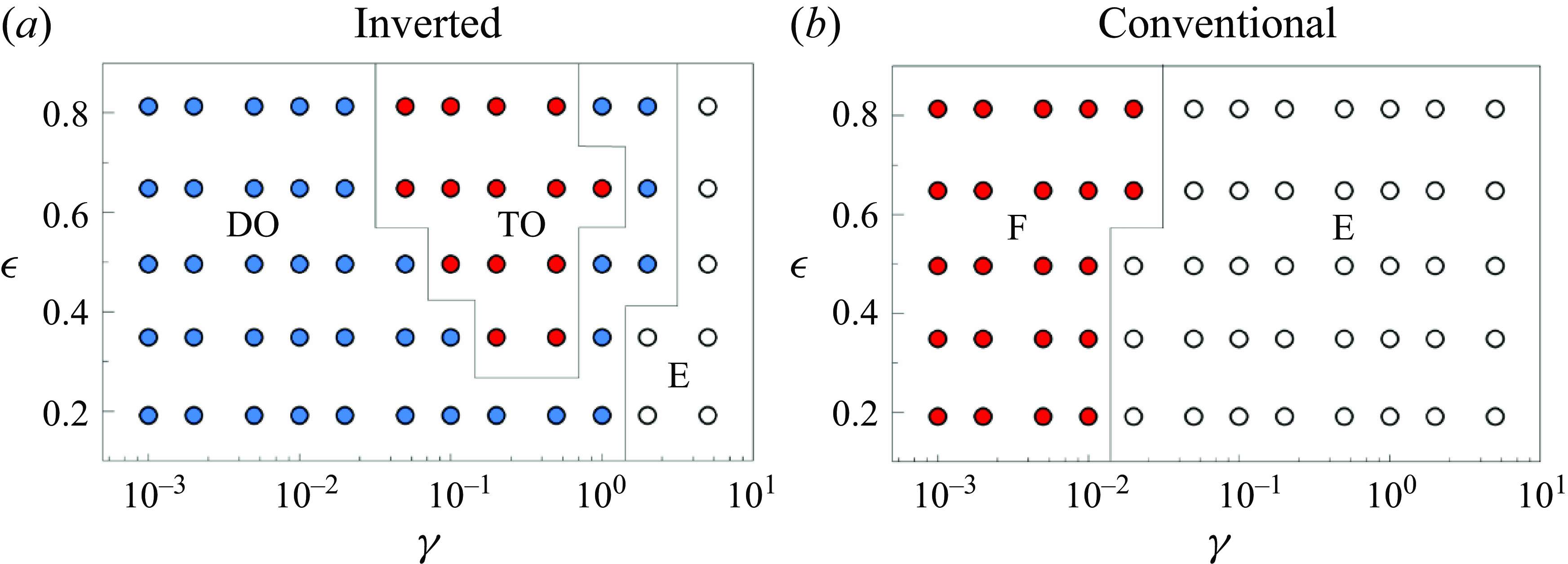
Figure 6. Mode diagram for (a) inverted and (b) conventional initial states depending on $\gamma$ and $\epsilon$ ; regions DO, TO, F and E correspond to the DO mode, the TO mode, the F mode and the E mode, respectively.

The TO mode of the inverted flexible ring, characterised by a large oscillation amplitude and high critical bending rigidity, is particularly well suited for energy harvesting. To better illustrate the TO mode, the time history of the midpoint ( $x_{{m}}$ , $y_{{m}}$ ), along with the sequential motion of the flexible ring, is presented in figure 7. From the time history of the midpoint, it is evident that the motion in the $y$ -direction dominates in the TO mode, whereas the $x$ -direction motion is almost negligible. Figure 7(b) depicts a complete TO mode cycle from $T_{0}$ to $T_{1}$ . At $T_{0}$ , $y_{{m}}$ is at its maximum value, signalling the beginning of a downward motion. By $T_{0}+\delta$ , the $y_{{m}}$ crosses the $x$ -axis, revealing an asymmetric shape. As the time progresses to $T_{0}+2\delta$ , $y_{{m}}$ reaches its minimum value, positioning the flexible ring at its lowest point. The ring then initiates an upward motion mirroring the earlier downward movement. Finally, at $T_{1}$ , the flexible ring returns to its upper position, marking the completion of one TO cycle.

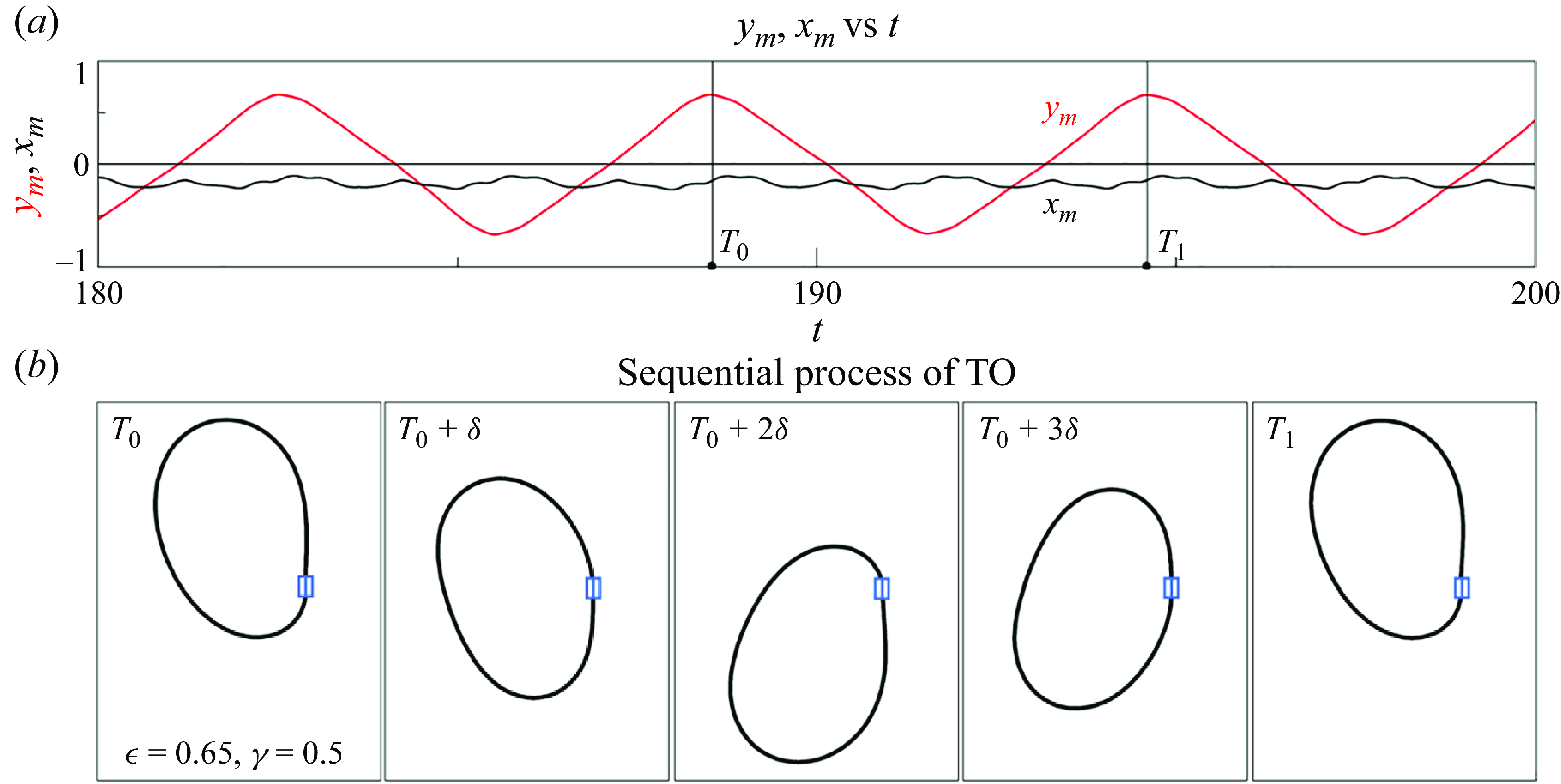
Figure 7. (a) Time histories of the midpoint ( $x_{{m}}$ , $y_{{m}}$ ) in the TO mode. (b) The sequential process of the TO mode ( $\epsilon = 0.65$ , $\gamma =$ 0.5).

We examined the vortex shedding and pressure distribution of the flexible ring across different modes. Figure 8 shows the instantaneous contours of $\omega _{z}$ and $p$ for the F, DO and TO modes. Although all three modes exhibit a 2S wake pattern, the shapes of the shed vortices and the corresponding pressure fields differ. In the F mode, the interaction between the two closed shear layers and the adjacent vortices causes the vortices to stretch and diverge. This interaction suppresses the low-pressure regions in the wake as the vortices dissipate. In the DO mode, the distance between the two shear layers increases, reducing the interaction between the shedding vortices. This reduced interaction results in more concentrated vortices and increased vorticity. In addition, the low-pressure region in the DO mode is more prominent than in the F mode. In the TO mode, vorticity intensifies, leading to even lower wake pressure, likely due to greater fluctuations in fluid forces, which enhance the oscillation amplitude. A detailed analysis of vortex shedding for each mode is presented in subsequent sections.

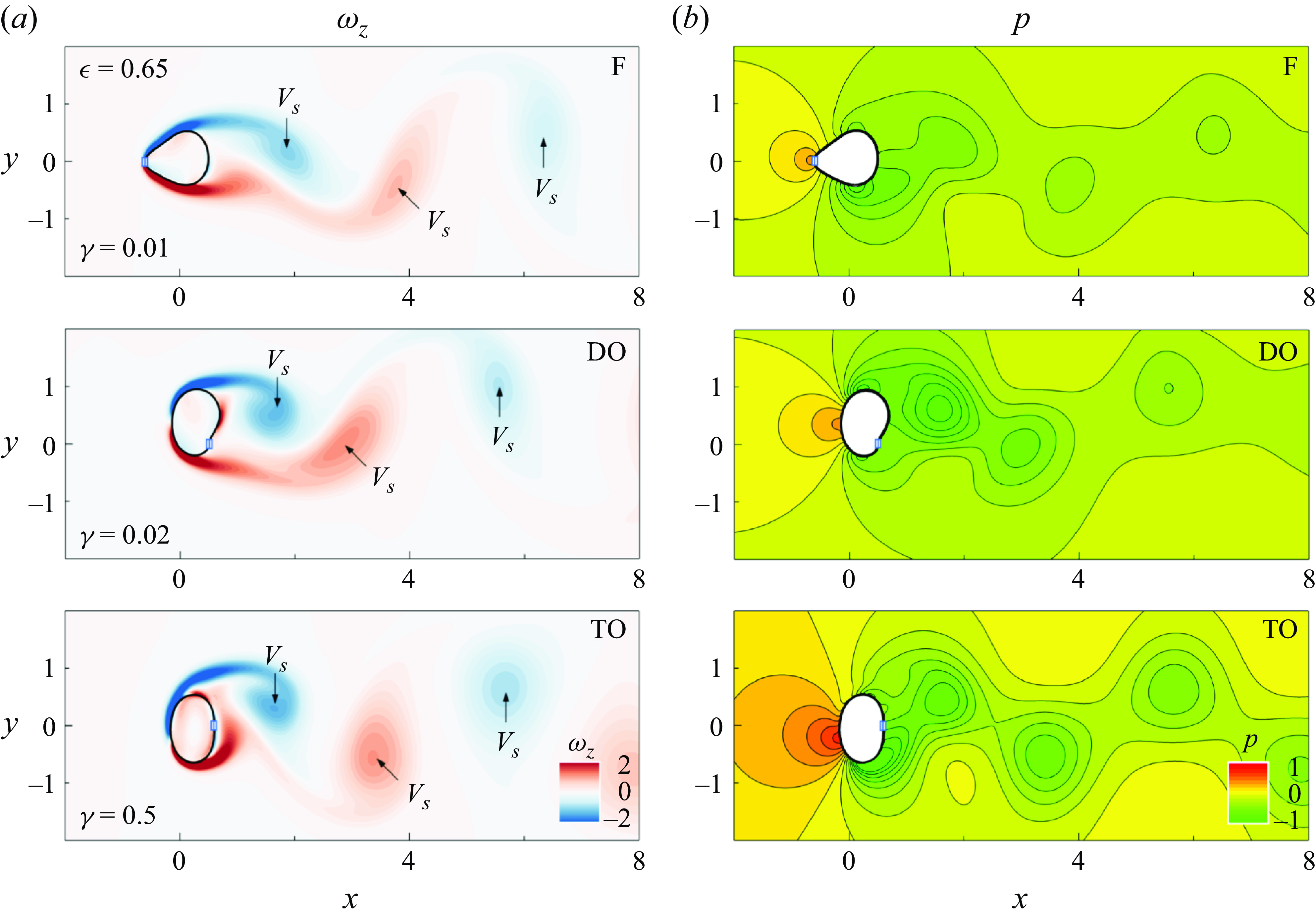
Figure 8. Instantaneous contours of (a) $\omega _{z}$ and (b) $p$ for the F mode ( $\gamma =0.01$ ), DO mode ( $\gamma =0.02$ ) and TO mode ( $\gamma =0.5$ ) under $\epsilon = 0.65$ .

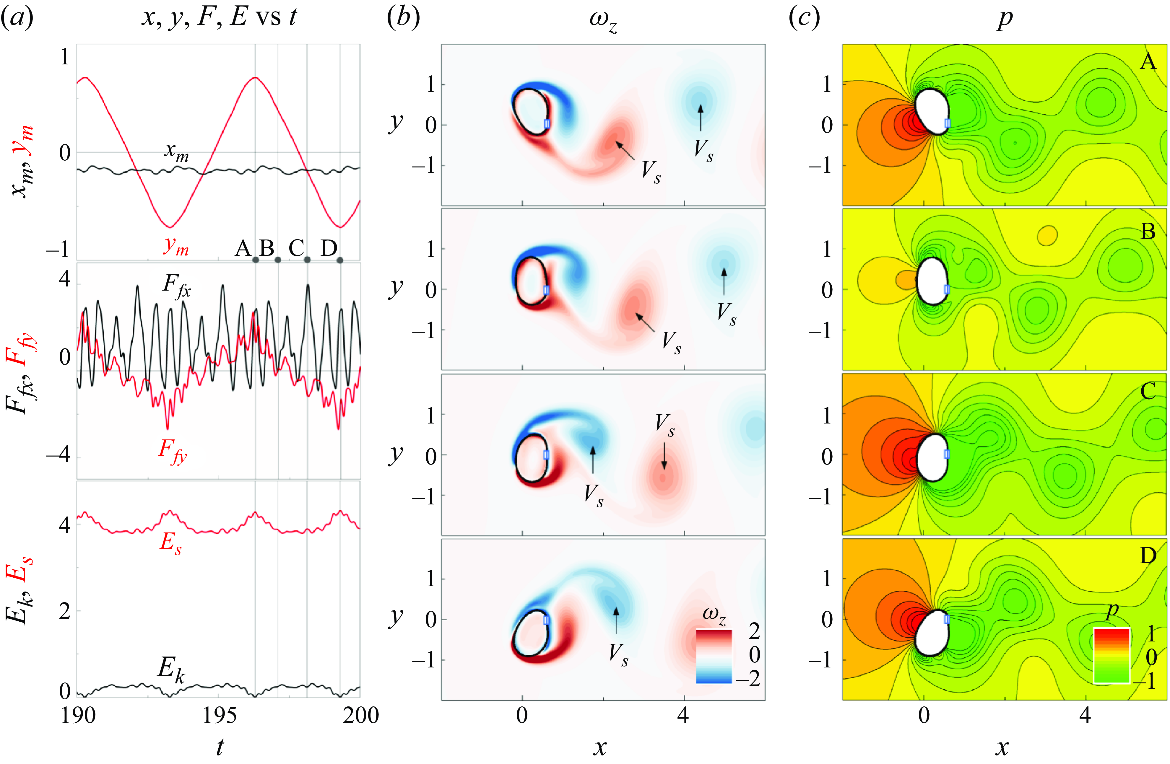
Figure 9. (a) Time histories of $x_{{m}}$ , $y_{{m}}$ , $F$ and $E$ . Instantaneous contours of (b) $\omega _{z}$ and (c) $p$ at A, B, C and D for $\epsilon = 0.65$ and $\gamma =$ 0.5 under the TO mode.

To elucidate the relationship between vortex shedding and ring motion, we analysed the vorticity and pressure contours around the flexible ring in the TO mode, alongside time histories of the midpoint position, fluid force, elastic force and energy (figure 9). Four specific time steps within one half of an oscillation period, denoted as A, B, C and D, are highlighted; the corresponding contours of $\omega _{z}$ and $p$ at these specific times are displayed in figure 9(b). Notably, the fluid force exhibits a higher-frequency component than the oscillation itself, likely because of the streamwise vibration of the ring. At time A, the flexible ring is in its uppermost position, with the $y_{{m}}$ at its maximum value. A high-pressure region forms on the lower-left side of the ring, whereas a low-pressure region, induced by vortex shedding, develops near the rear part. This pressure distribution results in a maximum value of $F_{{f}y}$ . The elastic energy ( $E_{{s}}$ ) also peaks because of the large deflection at this position. Simultaneously, a negative vortex is forming on the top of the ring and a positive vortex is being shed from it. After time A, the ring begins its downward motion, driven by the elastic restoring force. At time B, the high-pressure region diminishes and $F_{{f}y}$ approaches zero. Here, $E_{{s}}$ is largely converted into kinetic energy ( $E_{{k}}$ ), leading to a minimum in $E_{{s}}$ and a peak of $E_{{k}}$ . At time C, the $y_{{m}}$ passes the $x$ -axis, a negative vortex is shed, and a new high-pressure region forms on the upper-left side of the ring, generating a negative $F_{{f}y}$ that pushes the ring further downward. During the period from B to C, the elastic energy remains low, indicating minimal deformation. By time D, the ring reaches its lowest position, with elastic energy again at its maximum, mirroring the conditions at time A. After time D, the ring begins its upward motion, completing the oscillation cycle. The periodic formation and shedding of vortices play a critical role in driving the TO motion, with the associated fluid forces and pressure gradients directly influencing the ring’s dynamic behaviour.

3.2. Dimensional analysis of the energy equation

Having analysed the motion and wake patterns of the flexible ring across different modes, we here focus on the energy-harvesting performance. A dimensional analysis of the energy equation is applied to assess the contribution of each component to the overall energy-harvesting efficiency. By applying a Fourier transform to both sides of (2.20), we derive the energy equation in the frequency domain

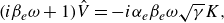(3.1) \begin{equation}(i\beta _{{e}}\omega +1)\hat{V}=-i\alpha _{{e}}\beta _{{e}}\omega \sqrt{\gamma }K,\end{equation}

where $\omega =2\pi f_{{y_{{m}}}}$ is the dominant angular frequency of the filament and $\hat{V}$ is the amplitude of the $V$ component with frequency $\omega$ . By combining Parseval’s theorem with (3.1), we can estimate the mean power coefficient $\overline{c}_{{p}}$ as

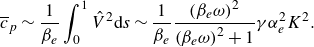(3.2) \begin{equation}\overline{c}_{{p}} \sim \frac{1}{\beta _{{e}}}\int _{0}^{1}\hat{V}^{2}\mathrm{d}s \sim \frac{1}{\beta _{{e}}}\frac{\left(\beta _{{e}}\omega \right)^{2}}{\left(\beta _{{e}}\omega \right)^{2}+1}\gamma \alpha _{{e}}^{2}K^{2}.\end{equation}

Given the small value of $\beta _{{e}}$ used in the present study, the expression simplifies to

(3.3) \begin{equation}\overline{c}_{{p}} \sim \gamma \beta _{e}\alpha _{{e}}^{2}\omega ^{2}K^{2}.\end{equation}

From this analysis, we can directly assess the influence of bending rigidity, oscillation frequency and filament deformation on energy harvesting. Deformation and oscillation frequency are critical because $\overline{c}_{{p}}$ is proportional to the square of the ring’s curvature. This relationship suggests that motion involving both high frequency and large deflection substantially enhances energy harvesting. Although $\overline{c}_{{p}}$ is only linearly proportional to $\gamma$ , the operational range of $\gamma$ spans several orders of magnitude, which closely affects $\overline{c}_{{p}}.$ The following sections examine the influence of bending rigidity and eccentricity on the flexible ring’s motion and energy-harvesting performance. Using prior analysis, we assess the contributions of bending rigidity, deflection and oscillation frequency to the efficiency of energy extraction from fluid–structure interactions.

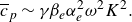
3.3. Effect of bending rigidity

We investigate the effect of bending rigidity on the dynamic and energy-harvesting performance of the clamped flexible ring, with eccentricity ( $\epsilon$ ) fixed at 0.65 for clarity. For comparison, results for transversely and streamwise buckled filaments are also included (Mao et al. 2024; Chen et al. 2024). Figure 10 illustrates the oscillation amplitude $(A_{y})$ and frequency $(f_{{y_{{m}}}})$ for both conventional and inverted flexible rings as $\gamma$ is varied. At low bending rigidity, the flexible ring is too soft to withstand the fluid forces, resulting in a deflected motion confined to one side and sustained in the DO mode, with a Strouhal number of ∼0.163. In this mode, $A_{y}$ is small, whereas $f_{{y_{{m}}}}$ is relatively high. As $\gamma$ increases to 0.05, the inverted ring transitions from the DO mode to the TO mode, leading to a sudden increase in $A_{y}$ , indicating the onset of large-amplitude motion. The Strouhal number in the TO mode is approximately 0.15, slightly lower than that in the DO mode. Notably, the oscillation frequency decreases after the transition. As $\gamma$ continues to increase, both $A_{y}$ and $f_{{y_{{m}}}}$ increase, reaching their maximum values at 0.2 and 0.5, respectively. The lock-in and resonance phenomena are observed near $\gamma =$ 0.5, where the oscillation frequency aligns with the vortex shedding frequency, suggesting that the TO mode exhibits vortex-induced vibration (VIV). This phenomenon resembles the lock-in behaviour observed in elastically mounted cylinders (Williamson & Govardhan 2004; Prasanth & Mittal 2008; Navrose & Mittal 2016) because of their similar geometries. Beyond the lock-in regime, both amplitude and frequency decrease, resulting in a transition to the E mode. By contrast, for the conventional clamped ring, vigorous motion occurs under low bending rigidity, with the vortex shedding frequency being twice the oscillation frequency for $\gamma \lt$ 0.01. Once $\gamma$ exceeds 0.01, the oscillation of the conventional ring synchronises with the vortex shedding. As $\gamma$ increases further, $A_{y}$ decreases, ultimately approaching zero at $\gamma =$ 0.1, indicating a transition to the E mode. The conventional ring does not demonstrate a lock-in phenomenon across various $\gamma$ , suggesting that its F mode is not VIV. This comparison reveals that the inverted ring exhibits a larger oscillation amplitude, higher frequency and greater bending rigidity in the lock-in regime compared with both transversely and streamwise buckled filaments, leading to superior energy-harvesting potential. Consequently, the following discussion focuses on the inverted-clamped filament.

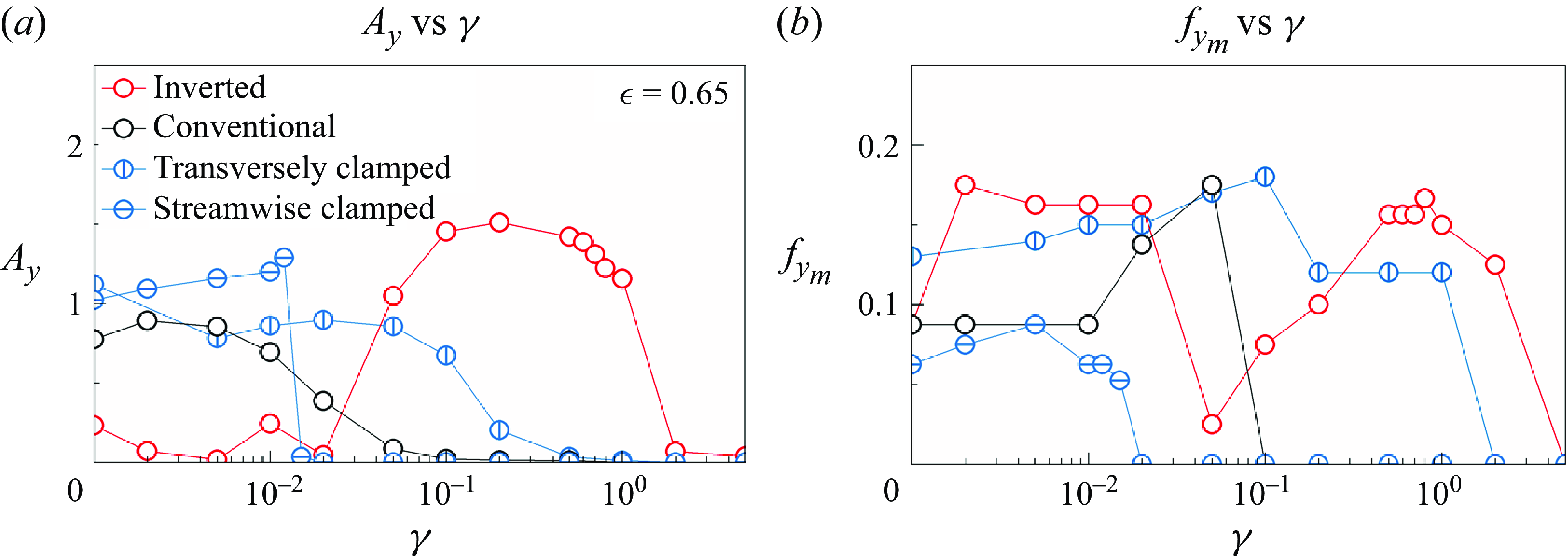
Figure 10. (a) Oscillation amplitude ( $A_{y}$ ) and (b) oscillation frequency ( $f_{{y_{{m}}}}$ ) as a function of $\gamma$ ( $\epsilon = 0.65$ ).

To further explore the transition between the DO and TO modes of the inverted ring, we examine the instantaneous contours of vorticity ( $\omega _{z}$ ) and the corresponding power spectral density (PSD) of both $f_{{y_{{m}}}}$ and $f_{v}$ in the transition region (figure 11). At $\gamma = 0.02$ , the inverted ring is in the DO mode, exhibiting a 2S wake pattern. In this mode, the DO motion is synchronised with the vortex shedding, as indicated by a peak at the same frequency in the PSD analysis. As $\gamma$ increases to 0.1, the inverted ring transitions to the TO mode. Although the wake pattern is similar to that observed at $\gamma =$ 0.02, a notable difference is observed: $f_{{y_{{m}}}}$ is lower than $f_{v}$ , indicating that the TO and vortex shedding are no longer synchronised. This desynchronisation contributes to the sudden decrease in $f_{{y_{{m}}}}$ observed in figure 10. At $\gamma =$ 0.5, the inverted ring enters a lock-in regime, where $f_{{y_{{m}}}}$ and $f_{v}$ match. The wake pattern in this regime shows a distinct gap between the positive and negative vortices in the $y$ -direction, whereas the vortices gather closely in the $x$ -direction, marking a clear change in the wake dynamics.

Figure 11. (a) Instantaneous contours of $\omega _{z}$ and (b) the PSD of $f_{{y_{{m}}}}$ and $f_{v}$ for an inverted-clamped ring under different $\gamma$ ( $\epsilon = 0.65$ ).

To further explore the interaction between the ring’s motion and vortex shedding, as well as to clarify the synchronisation phenomenon, we systematically analyse the oscillation frequency ( $f_{{y_{{m}}}}$ ), vortex shedding frequency ( $f_{v}$ ) and the natural frequency ( $f_{n}$ ) of the flexible ring as $\gamma$ varies, as illustrated in figure 12. The natural frequency is determined using the Euler–Bernoulli beam theory with clamped boundary conditions, yielding the formula $f_{n}=2.267\sqrt{\gamma /\rho _{s}}/2\pi$ . This analysis provides deeper insight into the coupling mechanisms governing the ring’s oscillations and its energy-harvesting potential. Figure 12 reveals that the different oscillation modes – F, DO and TO – are distinctly characterised by the relationships between the oscillation frequency, vortex shedding frequency and natural frequency. In the DO mode, the oscillation frequency matches the vortex shedding frequency while remaining different from the ring’s natural frequency. This observation suggests that the DO mode results from a simple forced vibration driven by unsteady fluid forces. In contrast, for the TO mode, the oscillation frequency initially increases with the natural frequency as $\gamma$ increases. Once the system enters the lock-in regime, the oscillation frequency synchronises with the vortex shedding frequency and maintains this synchronisation until the system exits the lock-in regime. This behaviour is reminiscent of VIV observed in elastically mounted cylinders, confirming that the TO mode is a form of VIV. Conversely, the F mode of the conventional ring does not exhibit any synchronisation, indicating that it is not associated with VIV. This distinction further highlights the different underlying mechanisms governing each oscillation mode.

Figure 12. Oscillation frequency ( $f_{{y_{{m}}}}$ ), vortex shedding frequency ( $f_{v}$ ) and natural frequency ( $f_{n}$ ) for (a) inverted rings and (b) conventional rings as a function of $\gamma$ ( $\epsilon = 0.65$ ).

We here shift our focus to the relationship between the ring’s motion and fluid force during the transition between the DO and TO modes. Figure 13 presents the time histories of the midpoint position ( $x_{{m}}$ , $y_{{m}}$ ) and the fluid force acting on the inverted ring under various $\gamma$ values. At $\gamma =$ 0.02, the inverted ring remains in the DO mode, characterised by small-amplitude, periodic motion and fluid force. As $\gamma$ increases to 0.1, the ring stores more elastic energy due to its higher bending rigidity. This enhanced energy storage allows the ring’s elastic restoring forces to more effectively counteract the fluid forces induced by vortex shedding, triggering the transition to the TO mode. This transition highlights the critical role of bending rigidity in governing the dynamic response of the flexible ring and its mode selection under varying flow conditions. In addition, the TO motion becomes aperiodic at $\gamma =$ 0.1. When $\gamma$ reaches 0.5, the inverted ring enters the lock-in regime, exhibiting large-amplitude, regular motion with a high oscillation frequency; this behaviour distinctly differs from that observed at $\gamma =$ 0.1. A high-frequency vibration in $x_{{m}}$ is evident, manifesting as a shaking motion in the ring during TO. In addition, the fluid force increases substantially compared with the values at $\gamma =$ 0.02 and 0.1, accompanied by a high-frequency component likely attributable to the vibrations in the $x$ -direction. The distinctive behaviour observed at $\gamma =$ 0.5 might be associated with the resonance of the inverted ring.

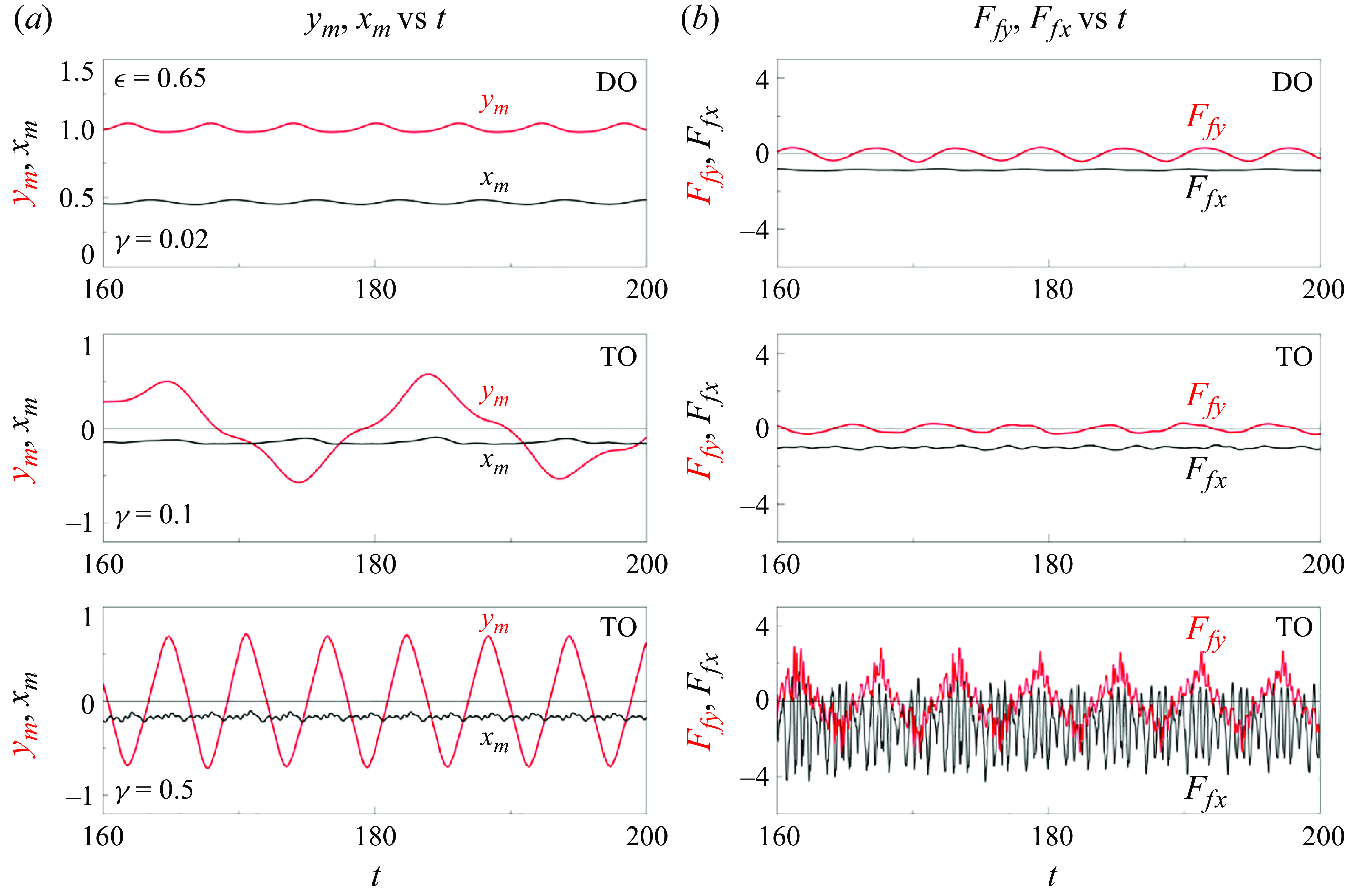
Figure 13. (a) Time histories of $x_{{m}}$ , $y_{{m}}$ , $F_{{f}x}$ and $F_{{f}y}$ of the inverted-clamped ring under different $\gamma$ ( $\epsilon = 0.65$ ).

Here, we analyse the degree of deformation and the variation in elastic energy, both of which are directly linked to energy-harvesting performance. Figure 14 illustrates the average variation of curvature ( $\overline{K}^{\prime}$ ) and elastic energy ( $\overline{E}_{s}^{\prime}$ ) for both inverted and conventional ring functions of $\gamma$ . Here, $\overline{K}^{\prime}$ is defined as $\overline{K}^{\prime}=\overline{K}-\overline{K}_{min }$ , where $\overline{K}=\int _{0}^{L}K(s,t)\mathrm{d}s$ represents the deflection during the ring’s motion. The time-averaged elastic energy $\overline{E}_{s}^{\prime}$ is defined as $\overline{E}_{s}^{\prime}=\overline{E}_{{s}}-\overline{E}_{{s}\,min }$ , indicating the elastic variation in the ring’s motion. Both $\overline{K}^{\prime}$ and $\overline{E}_{{s}}^{\prime}$ of the inverted ring remain low in the DO mode because the oscillation amplitudes are small (figure 10). When the motion transitions to the TO mode, both $\overline{K}^{\prime}$ and $\overline{E}_{s}^{\prime}$ increase, with $\overline{E}_{s}^{\prime}$ exhibiting a higher rate of increase than $\overline{K}^{\prime}$ , which we attribute to the influence of $\gamma$ on $\overline{E}_{s}^{\prime}$ (as shown in (2.21)). Both $\overline{K}^{\prime}$ and $\overline{E}_{s}^{\prime}$ reach their maximum values at $\gamma =$ 0.5, indicating resonance. Notably, the oscillation amplitude $A_{y}$ peaks at $\gamma =$ 0.2, which is slightly lower than the $\gamma$ corresponding to the peak of $\overline{K}^{\prime}$ , suggesting that oscillation amplitude does not accurately reflect the intensity of motion. After the inverted ring exits the lock-in regime, both $\overline{K}^{\prime}$ and $\overline{E}_{s}^{\prime}$ exhibit a sudden decrease. Conversely, for the conventional ring, although $A_{y}$ is relatively lower in the F mode than in the TO mode of the inverted ring, the values of $\overline{K}^{\prime}$ remain comparable. However, $\overline{K}^{\prime}$ is still lower than that of the TO mode because of the lower bending rigidity.

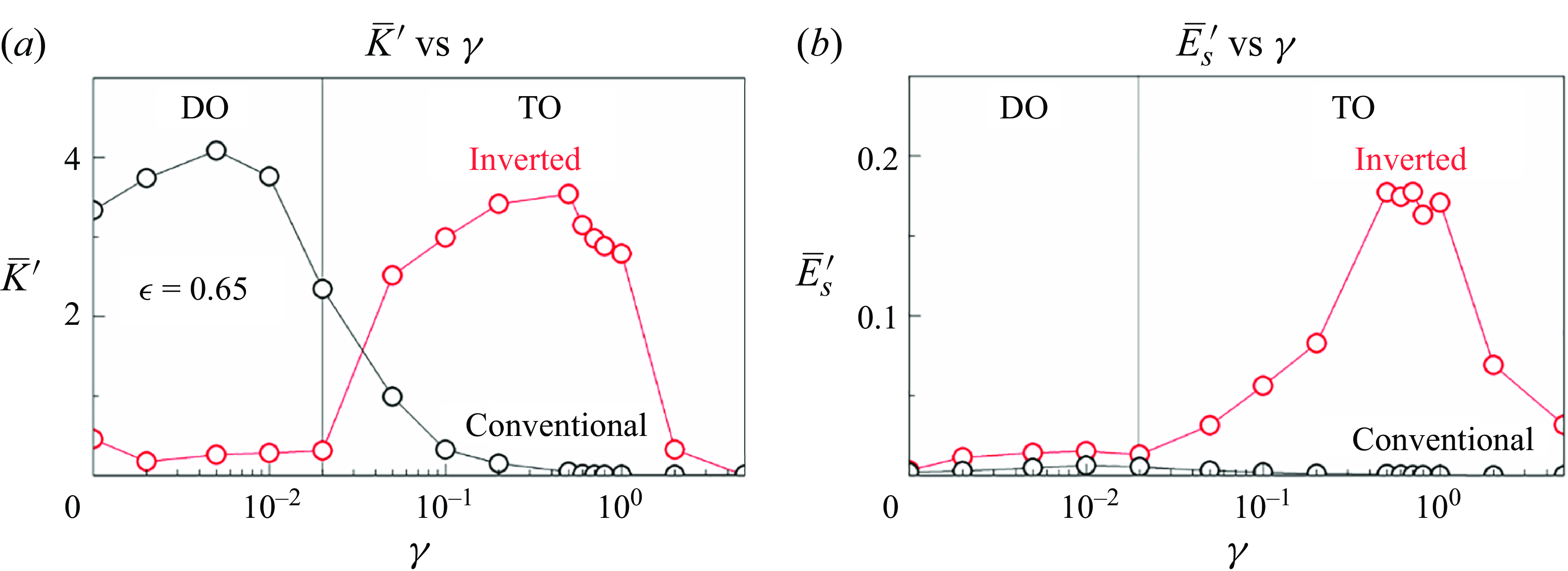
Figure 14. Average variation of (a) curvature ( $\overline{K}^{\prime}$ ) and (b) elastic energy ( $\overline{E}_{s}^{\prime}$ ) for inverted and conventional rings as a function of $\gamma$ ( $\epsilon = 0.65$ ).

To assess the deflection and elastic energy distribution of the inverted ring, we examine the local curvature variation $\langle K\rangle $ and the time-averaged strain energy $\langle E_{{s}}\rangle$ for different values of $\gamma$ (figure 15). The local curvature variation is defined as $\langle K\rangle = K_{max }-K_{min }$ , indicating the amplitude of curvature variation during oscillation, which is directly related to power generation. The time-averaged strain energy is defined as $\left\langle E_{{s}}\right\rangle =({1}/{T})\int _{0}^{T}E_{{s}}\mathrm{d}t$ , representing the elastic energy distribution of the mean shape. Most of the deflection occurs near the clamped edge of the inverted ring in the DO mode ( $\gamma =$ 0.02), leading to a concentration of elastic energy, making it ideal for attaching piezoelectric patches. In addition, the curvature is asymmetric, with higher values observed toward the trailing end of the ring, which is attributed to its deflected shape. The inverted ring shows similar $\langle K\rangle$ values for $\gamma =$ 0.2 and 0.5, both of which are in the TO mode. Although the $\gamma =$ 0.2 exhibits a larger $\langle K\rangle$ , the value of $\langle E_{{s}}\rangle$ at 0.5 is greater, reflecting the influence of greater $\gamma$ . Notably, the average elastic energy distribution differs from the curvature variation, indicating that greater deformations in the mean shape do not necessarily correlate with increased energy generation.

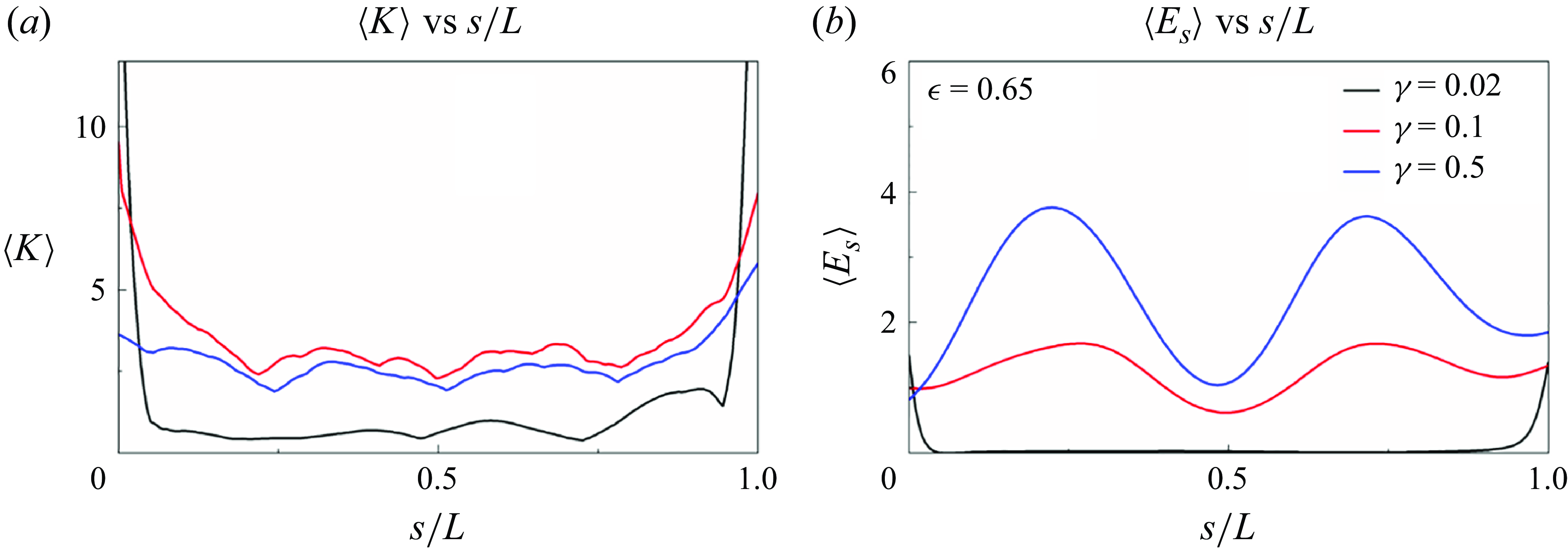
Figure 15. (a) Values of $\langle K\rangle$ and (b) $\langle E_{{s}}\rangle$ for an inverted ring as a function of $s/L$ ( $\epsilon = 0.65$ ).

We examine the average power coefficient ( $\overline{c}_{{p}}$ ) and its estimation using three components ( $\gamma (\overline{K}^{\prime}f_{{y_{{m}}}})$ ²) derived from the dimensional analysis (figure 16). The average power coefficient is defined as $\overline{c}_{{p}}=({1}/{LT})\int _{0}^{T}\int _{0}^{L}c_{{p}}\mathrm{d}s\mathrm{d}t$ . For comparison, results for both transversely and streamwise-clamped buckled filaments are also included (Mao, Liu & Sung 2024; Chen et al. 2025). The trend of $\gamma (\overline{K}^{\prime}f_{{y_{{m}}}})^{2}$ closely resembles that of $\overline{c}_{{p}}$ , indicating that it serves as a good approximation for $\overline{c}_{{p}}$ and validating our analysis in § 3.2. The $\overline{c}_{{p}}$ of the inverted ring in the DO mode is nearly negligible, which is attributable to the low amplitude and bending rigidity of this mode. Upon transitioning from the DO mode to the TO mode, the inverted ring exhibits an increase in oscillation amplitude, although $\overline{c}_{{p}}$ remains low because of the low values of $\gamma$ and $f_{{y_{{m}}}}$ . When the inverted ring enters the lock-in regime, $\overline{c}_{{p}}$ increases sharply and maintains a high value throughout this regime; this behaviour results from the large-amplitude and high-frequency oscillations of the inverted ring. In addition, the high bending rigidity contributes to the elevated $\overline{c}_{{p}}$ . Once the inverted ring exits the lock-in regime, $\overline{c}_{{p}}$ experiences a substantial decrease, reflecting the reductions in $\overline{K}^{\prime}$ and $f_{{y_{{m}}}}$ . By contrast, although the $\overline{K}^{\prime}$ in the F mode of a conventional ring is comparable to that in the TO mode, the lower bending rigidity results in a consistently low $\overline{c}_{{p}}$ . For the streamwise-clamped buckled filament, substantial deflection occurs during its STO mode; however, low critical bending rigidity and low frequency limit its $\overline{c}_{{p}}$ . The transversely clamped buckled filament enhances the critical bending rigidity and the oscillation frequency, leading to a higher $\overline{c}_{{p}}$ compared with that of the streamwise configuration. Ultimately, the TO mode of the inverted ring, characterised by a large oscillation amplitude, high frequency and substantial critical bending rigidity, achieves the highest $\overline{c}_{{p}}$ , indicating significant potential for energy harvesting.

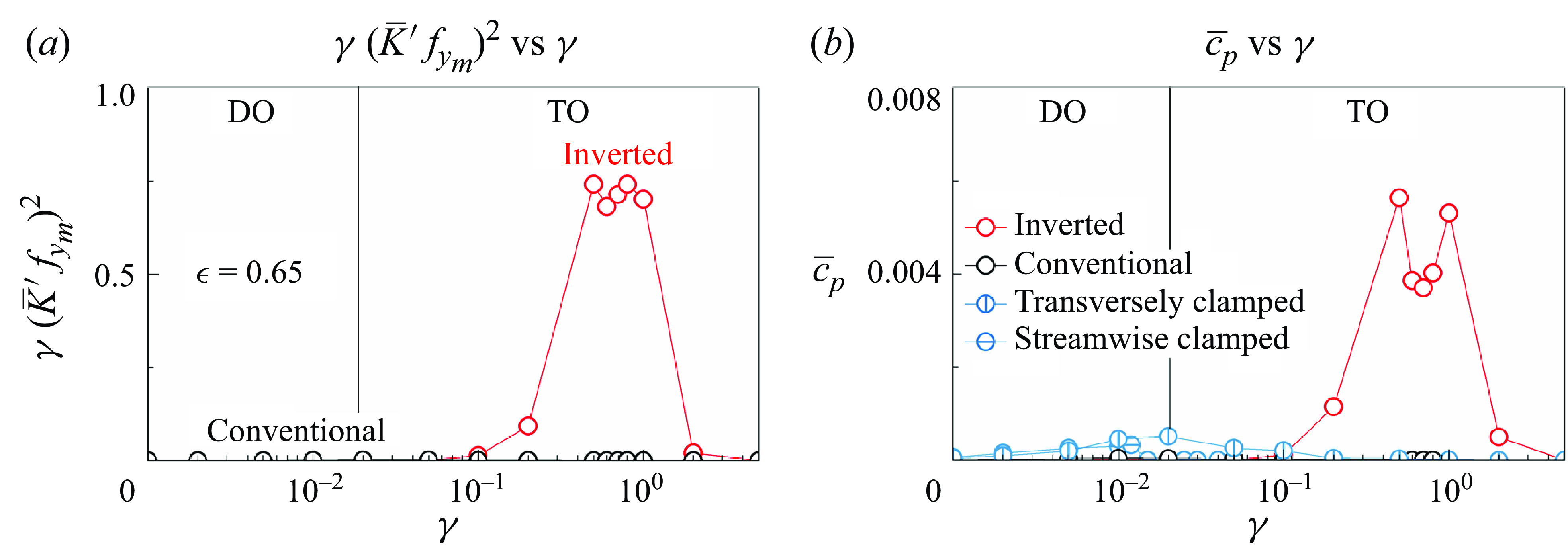
Figure 16. (a) Values of $\gamma (\overline{K}^{\prime}f_{{y_{m}}})^{2}$ and (b) the average power coefficient ( $\overline{c}_{p}$ ) as a function of $\gamma$ (0.65).

Finally, a direct comparison of oscillation behaviour and energy-harvesting performance between the inverted ring and the inverted flag is essential. In the inverted flag, although some lock-in characteristics are present, the oscillation frequency continuously increases with increasing bending rigidity or flow velocity (Ryu et al. 2015; Shoele & Mittal 2016; Kim, Kang & Kim 2017). In contrast, the inverted ring closely follows classical VIV behaviour, with its oscillation frequency locking near the natural frequency within the lock-in regime. Notably, the inverted ring exhibits a distinct high-frequency vibration within the lock-in region (figures 9 and 13), which is absent in the inverted flag. This high-frequency component, driven by rapid vibrations and significant curvature variations, enhances energy-harvesting efficiency. As shown in figure 17, the average power coefficient ( $\overline{c}_{{p}}$ ) of the inverted ring is 5–10 times higher than that of the inverted flag under identical conditions. Although the power coefficient ( $c_{{p}}$ ) of the inverted flag fluctuates with the flapping cycle, the inverted ring maintains stable high-frequency components in $c_{{p}}$ , directly contributing to its superior performance.

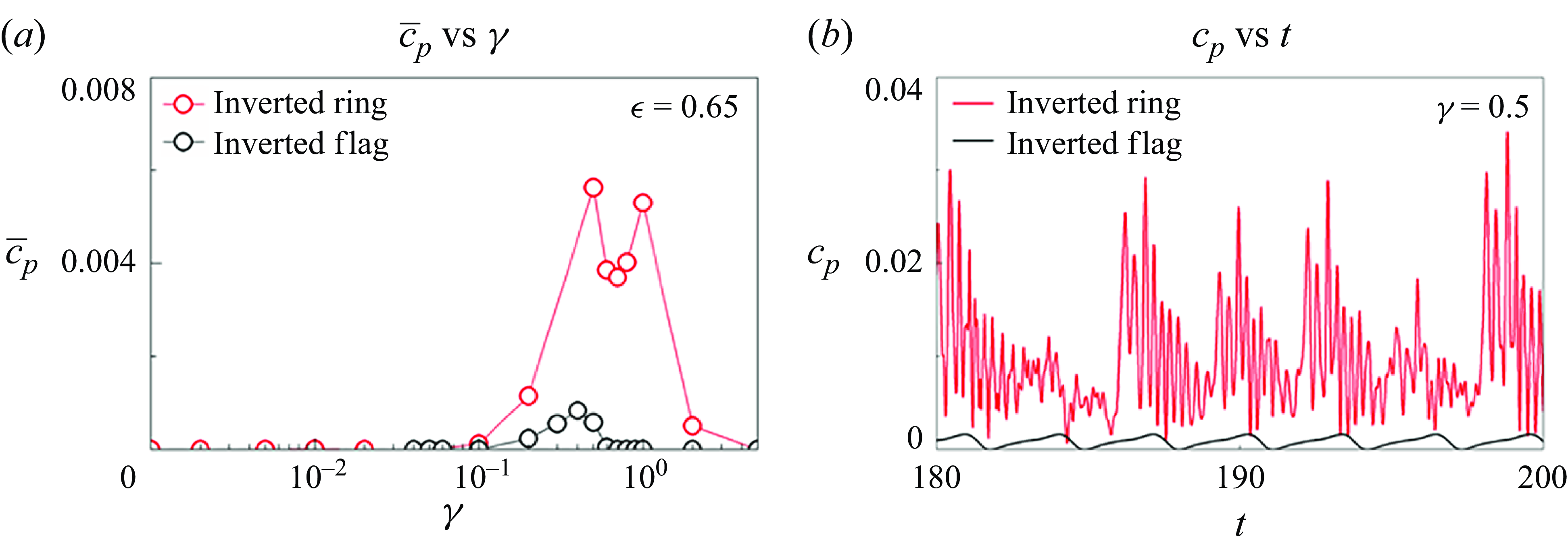
Figure 17. (a) Variation of the average power coefficient ( $\overline{c}_{{p}}$ ) as a function of $\gamma$ , and (b) time evolution of the power coefficient ( $c_{{p}}$ ) for the inverted ring and inverted flag.

3.4. Effects of eccentricity

The eccentricity of the initial shape influences the volume enclosed by the flexible ring, thereby affecting its shape and motion. A high eccentricity suggests the ring is closer to a circular shape, whereas a low eccentricity indicates a more slender, elongated configuration. In this section, we examine the effect of eccentricity on the dynamic behaviour and energy-harvesting performance of the clamped ring. The bending rigidity is set to 0.5 for the inverted ring and 0.01 for the conventional ring, ensuring that the inverted ring predominantly operates in the TO mode, whereas the conventional ring remains in the F mode. Figure 18 illustrates the superposition of the instantaneous shapes of the flexible ring under various eccentricities in the TO mode. When $\epsilon = 0.65$ , the ring’s shape becomes increasingly flat, deviating from circularity. This alteration reduces the constraints imposed by inextensibility and volume conservation, resulting in vigorous motion. As $\epsilon$ increases to 0.7, the oscillation amplitude decreases slightly while still maintaining a large value. The rationale for initially selecting $\epsilon = 0.65$ is now being revisited. At $\epsilon = 0.88$ , the oscillation amplitude further diminishes, indicating small-amplitude oscillations. Finally, at $\epsilon = 1$ , which corresponds to a perfect circle, the ring remains steady because of the limitations imposed by the inextensibility condition, mass conservation and clamped edges.

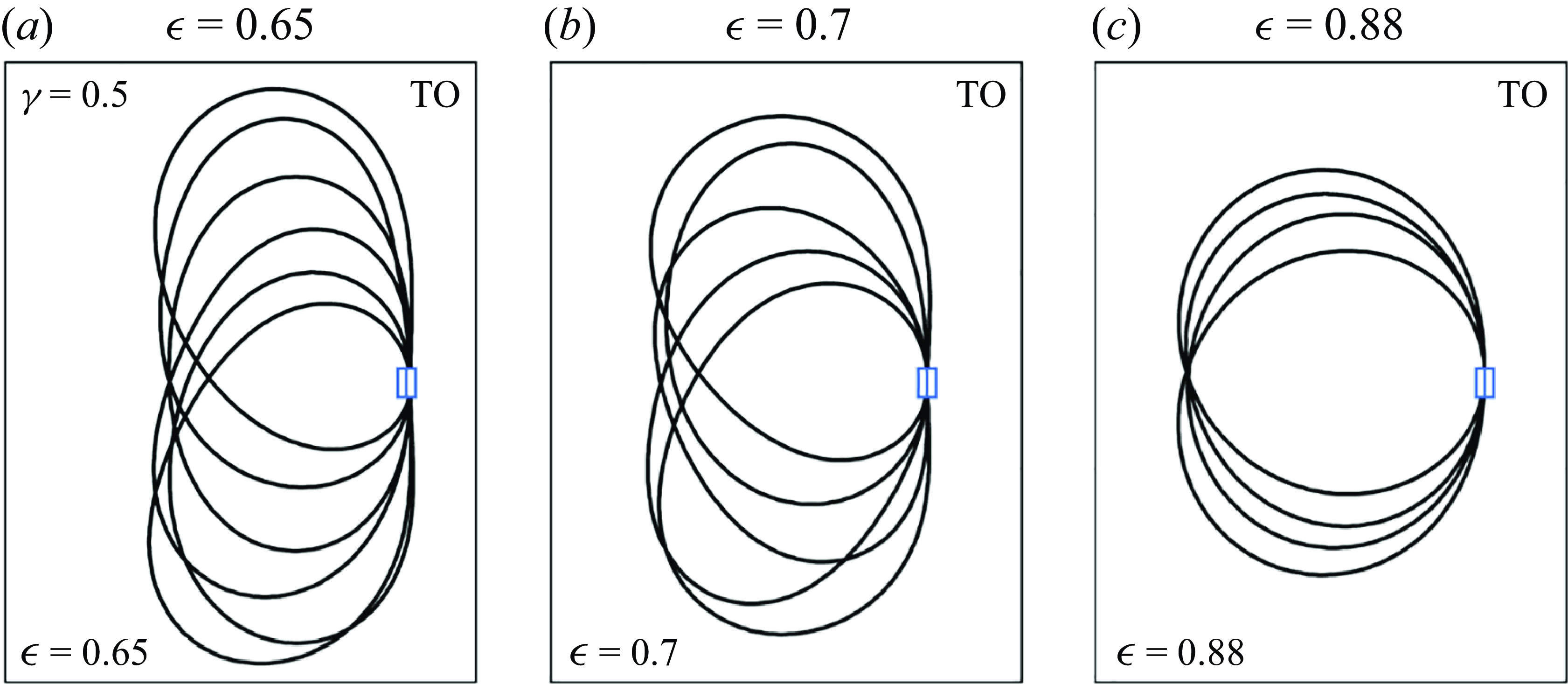
Figure 18. Superposition of the instantaneous shapes of inverted rings under different $\epsilon$ ( $\gamma =$ 0.5).

To further investigate the effect of $\epsilon$ on the dynamics of the clamped ring, we examine the oscillation amplitude and frequency as functions of $\epsilon$ (figure 19). At $\epsilon = 0.2$ , the inverted ring operates in the DO mode, characterised by low amplitude and high frequency. As $\epsilon$ increases to 0.25, the inverted ring transitions to the TO mode, resulting in a substantial increase in $A_{y}$ . However, this larger amplitude is achieved at the cost of a reduced operational range for the TO mode, indicating that activation becomes more challenging at higher $\epsilon$ (figure 6). When $\epsilon$ reaches 0.4, the ring enters the lock-in regime, where the oscillation frequency matches the vortex shedding frequency. As $\epsilon$ continues to increase, the oscillation amplitude decreases because of increased volume restrictions. When $\epsilon$ reaches 1, the amplitude decreases to zero, indicating a transition to the E mode. By contrast, the conventional clamped ring exhibits large-amplitude motion at $\epsilon = 0.2$ and does not display a DO mode, differing from the inverted configuration. Like the inverted ring, the conventional ring exhibits a decrease in oscillation amplitude with increasing $\epsilon$ . In summary, $\epsilon$ substantially affects the oscillation intensity and the presence of the TO mode in the inverted ring, where higher values favour the TO mode while suppressing oscillation intensity.

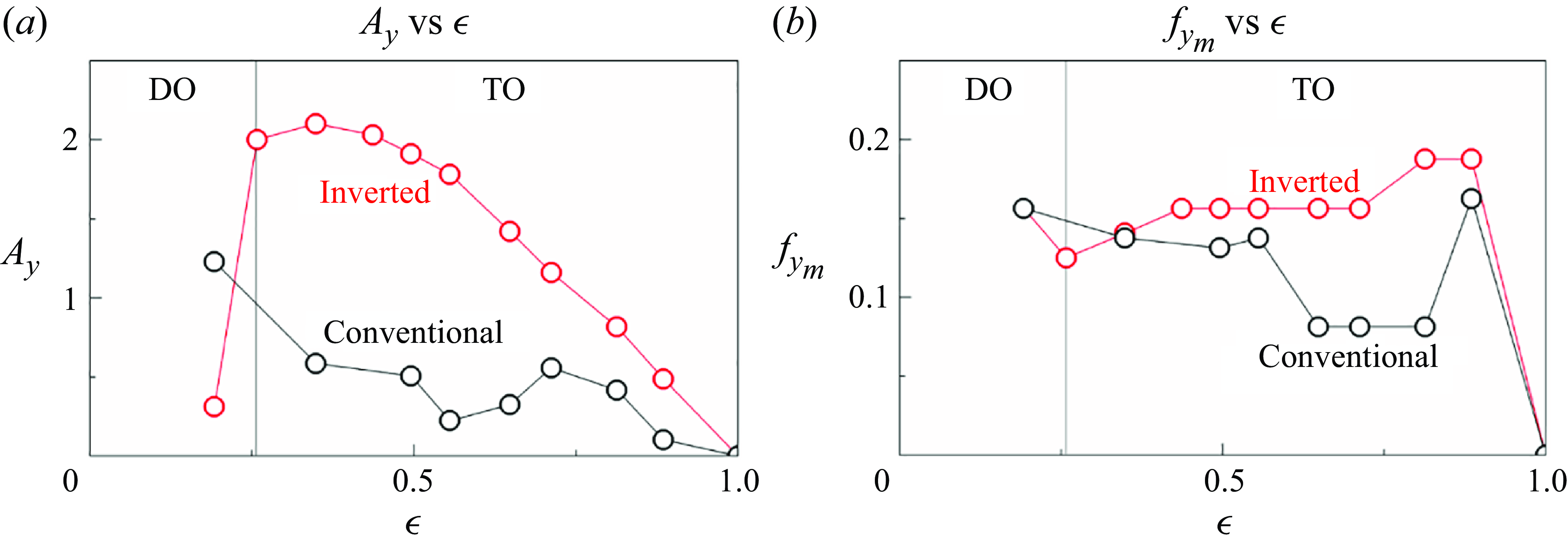
Figure 19. (a) Values of $A_{y}$ and (b) $f_{{y_{{m}}}}$ for inverted and conventional rings as a function of $\epsilon (\gamma =$ 0.5 for inverted and $\gamma =$ 0.01 for conventional).

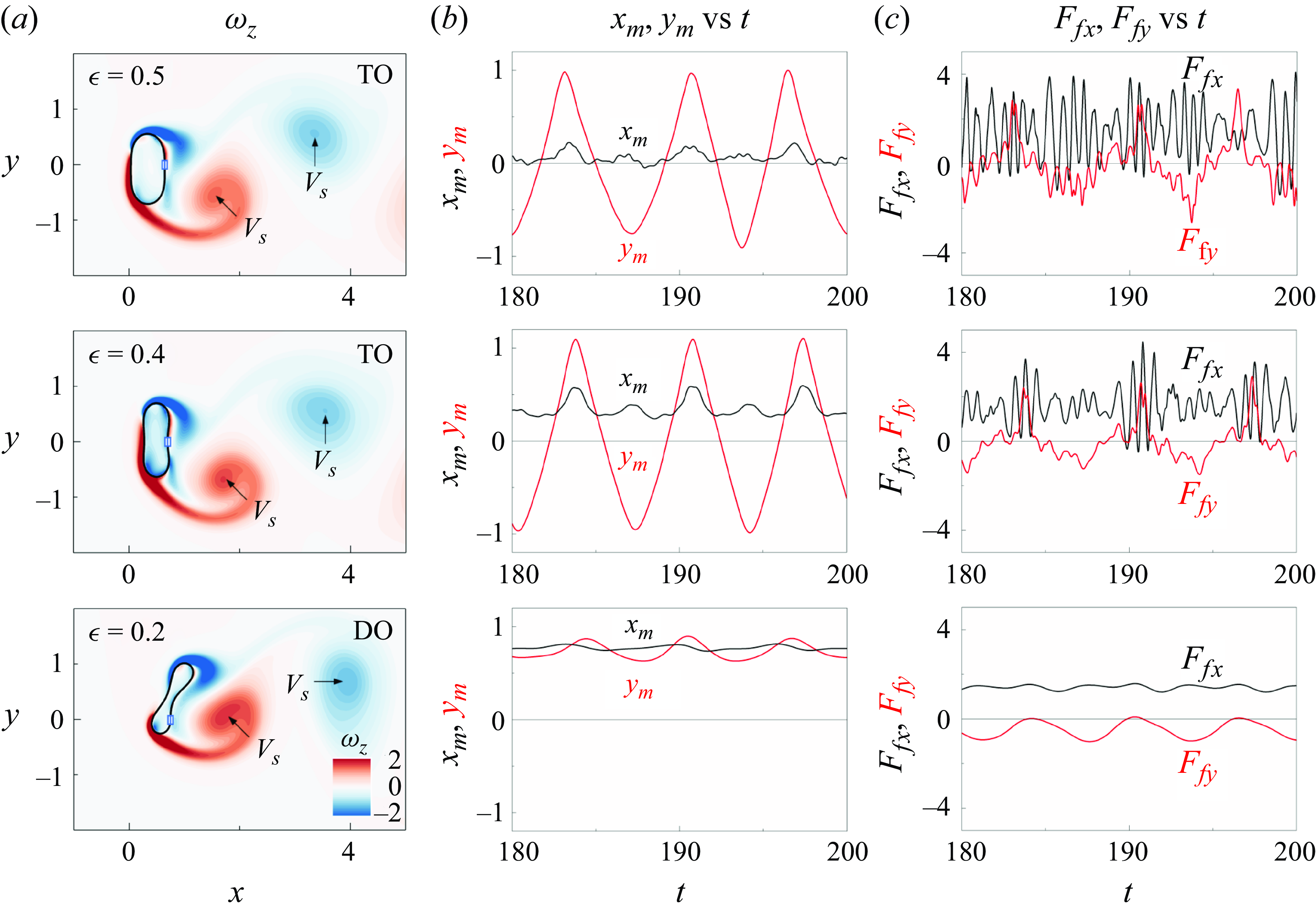
Figure 20. (a) Instantaneous contours of $\omega _{z}$ and time histories of (b) the midpoint displacement and (c) fluid force for an inverted ring under $\epsilon = 0.5$ , 0.4, 0.2 ( $\gamma =$ 0.5).

To investigate the transition from the TO mode to the DO mode as $\epsilon$ varies, we display the vorticity contours alongside the time history of the midpoint displacement and fluid force in figure 20. At $\epsilon = 0.5$ , the ring remains in the TO mode, characterised by a 2S wake pattern. A high-frequency component in $x_{{m}}$ suggests streamwise shaking of the ring during TO motion, likely caused by high-frequency variations in the streamwise fluid force $F_{{f}x}$ . As $\epsilon$ decreases to 0.4, the ring becomes flatter, resulting in a higher oscillation amplitude. The motion of the ring at $\epsilon = 0.4$ appears more regular than that at $\epsilon$ = 0.5. When $\epsilon$ further decreases to 0.2, the flatness of the ring increases, causing a transition to the DO mode. The DO mode at $\epsilon$ = 0.2 resembles the flapping motion observed in transversely clamped filaments (Kwon et al. 1992; Lee et al. 2017, 2018; Wang et al. 2020). The primary mechanism behind the disappearance of the TO mode at lower $\epsilon$ is the reduction in the transverse elastic restoring force. As $\epsilon$ decreases, the ring flattens and tilts further downstream, which redirects a larger portion of its elastic force to counteract the streamwise fluid forces. This reallocation leaves insufficient restoring force in the transverse direction to return the ring to its centred position, thus preventing the exhibition of the TO mode.

We here focus on the deformation and elastic energy of the inverted and conventional rings under various $\epsilon$ (figure 21). The behaviour of $\overline{K}^{\prime}$ follows a trend similar to $A_{y}$ as $\epsilon$ varies. Specifically, $\overline{K}^{\prime}$ increases as $\epsilon$ decreases, reaching a critical point where the inverted ring shifts to the DO mode, causing a sharp decrease in $\overline{K}^{\prime}$ . The trend of $\overline{E}_{s}^{\prime}$ generally follows that of $A_{y}$ , with one key distinction: $\overline{E}_{s}^{\prime}$ peaks at $\epsilon = 0.4$ , whereas both $\overline{K}^{\prime}$ and $A_{y}$ peak at $\epsilon = 0.25$ . These results suggest that, as the ring flattens further, large deformations become increasingly difficult. Although the inverted ring achieves the highest $\overline{E}_{s}^{\prime}$ under $\epsilon = 0.4$ , the narrow range of the TO mode limits its suitability for energy harvesting. For the conventional ring, deformation continues to increase as $\epsilon$ decreases, with $\overline{K}^{\prime}$ reaching a substantial value at $\epsilon = 0.2$ . Although the $\overline{K}^{\prime}$ of the conventional ring is comparable to that of the inverted ring, its notably lower bending rigidity results in negligible $\overline{E}_{s}^{\prime}$ relative to the inverted configuration.

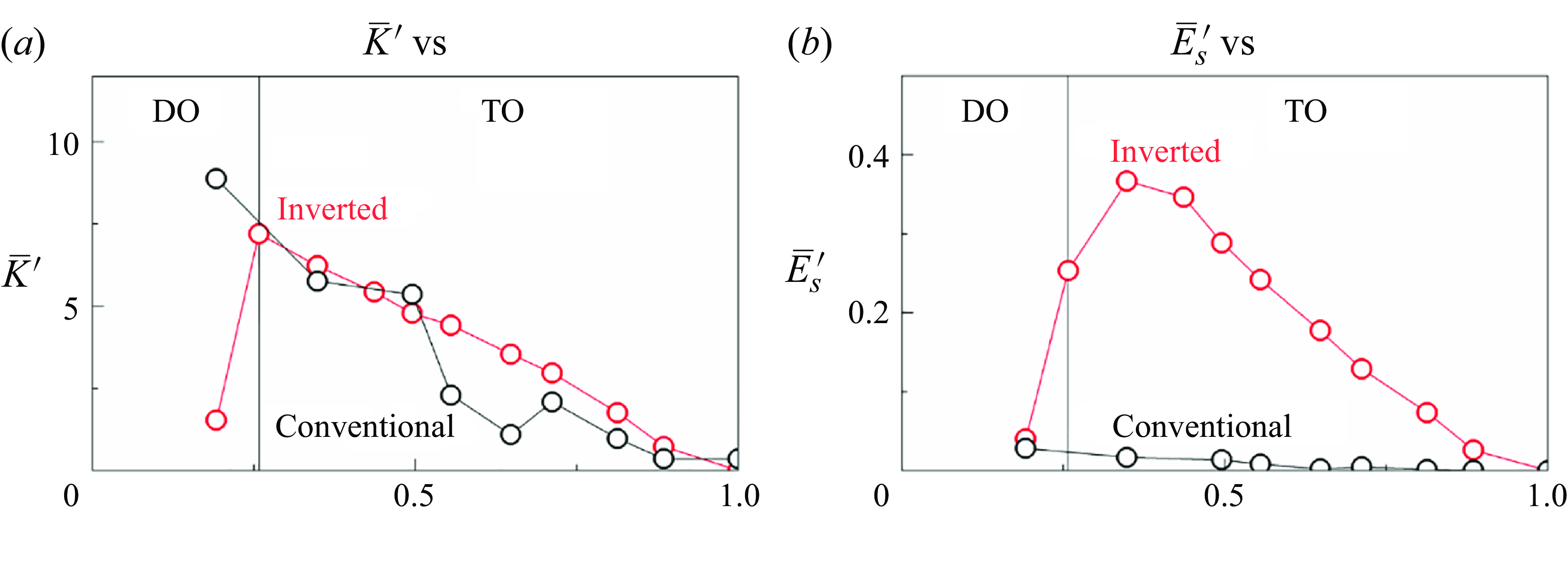
Figure 21. (a) Average variation of curvature ( $\overline{K}^{\prime}$ ) and (b) elastic energy ( $\overline{E}_{s}^{\prime}$ ) for inverted and conventional rings as a function of $\epsilon$ ( $\gamma =$ 0.5 for inverted and $\gamma =$ 0.01 for conventional).

Next, we examine $\langle K\rangle$ and $\langle E_{{s}}\rangle$ as functions of $s/L$ under various $\epsilon$ to understand the curvature and average deformation across each segment of the ring (figure 22). The inverted ring maintains the TO mode under $\epsilon = 0.4$ and 0.5, resulting in similar distributions of $\langle K\rangle $ and $\langle E_{{s}}\rangle$ . However, $\langle K\rangle$ and $\langle E_{{s}}\rangle$ are generally larger at $\epsilon = 0.4$ than at $\epsilon = 0.5$ , indicating greater deformation at $\epsilon = 0.4$ , as also shown in figure 20. As $\epsilon$ decreases to 0.2, the ring shifts to DO mode. Notably, $\langle K\rangle$ in the DO mode is lower than in the TO mode, whereas $\langle E_{{s}}\rangle$ is higher. This difference indicates that, although the DO mode displays greater average deformation because its deflected shape, the intensity of motion is relatively low. In addition, the ring’s deflected shape results in an asymmetric distribution of $\langle E_{{s}}\rangle$ .

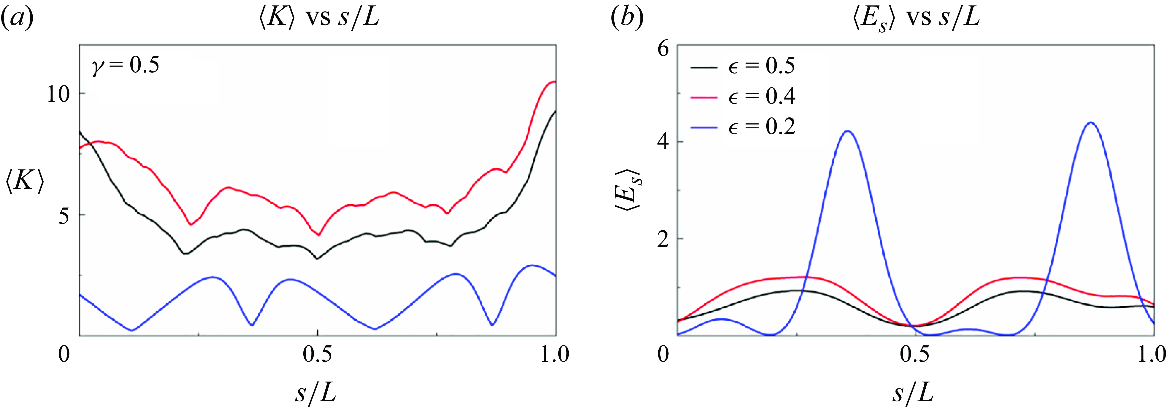
Figure 22. (a) Values of $\langle K\rangle $ and (b) $\langle E_{{s}}\rangle$ as functions of $s/L$ for an inverted ring under different $\epsilon$ ( $\gamma =$ 0.5).

We here examine the influence of $\epsilon$ on the power coefficient estimate, $\gamma (\overline{K}^{\prime}f_{{y_{{m}}}})$ ², and the average power coefficient, $\overline{c}_{{p}}$ in figure 23. At $\epsilon = 1$ , the inverted ring remains stationary because of volume and length constraints, leading to $\overline{c}_{{p}}=$ 0. As $\epsilon$ increases, these constraints relax, allowing for increased dynamic motion and an increase in $\overline{c}_{{p}}$ . For $\epsilon$ > 0.7, $\overline{c}_{{p}}$ remains low, which is attributable to small oscillation amplitudes and a reduced $\overline{K}^{\prime}.$ When $\epsilon$ reaches 0.65, the oscillation amplitude becomes sufficiently large to increase $\overline{c}_{{p}}$ . Within the range 0.34 $\leq \epsilon \leq$ 0.65, $\overline{c}_{{p}}$ remains high, indicating optimal energy-harvesting performance. However, $\gamma (\overline{K}^{\prime}f_{{y_{{m}}}})$ ² underestimates $\overline{c}_{{p}}$ in this range, likely because $\overline{K}^{\prime}$ overestimates ring deflection. As the ring shifts from the TO mode to the DO mode, $\overline{c}_{{p}}$ decreases sharply, corresponding to a reduction in $\overline{K}^{\prime}$ . Considering both $\overline{c}_{{p}}$ and the TO mode range, the optimal $\epsilon$ for energy harvesting is 0.65. In comparison, the conventional ring’s low bending rigidity results in consistently low $\overline{c}_{{p}}$ values across all $\epsilon$ , rendering it less effective for energy harvesting than the inverted configuration.

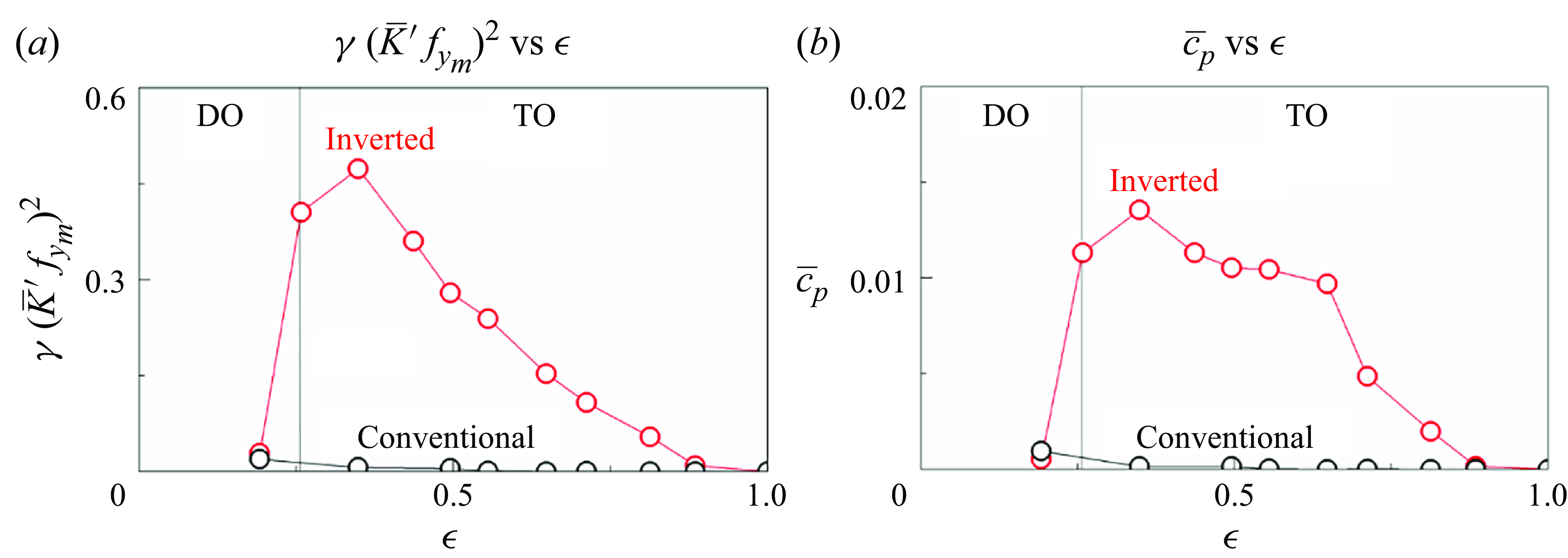
Figure 23. (a) Values of $\gamma (\overline{K}^{\prime}f_{{y_{{m}}}})$ ² and (b) average power coefficient ( $\overline{c}_{{p}}$ ) for inverted and conventional rings as a function of $\epsilon$ ( $\gamma =$ 0.5 for inverted and $\gamma =$ 0.01 for conventional).

4. Conclusions

We investigated the flow-induced oscillations of a clamped flexible ring using the penalty IB method, examining both inverted and conventional configurations. The effects of bending rigidity and eccentricity on the ring’s dynamics were systematically analysed. Our study identified four distinct oscillation modes as these parameters were varied: the F mode, DO mode, TO mode and E mode. Each mode exhibited a 2S wake pattern. In the inverted configuration, the ring maintained the DO mode at low $\gamma$ values, characterised by a deflected shape. As $\gamma$ increased, the ring transitioned to the TO mode, which displayed large-amplitude oscillations and a lock-in phenomenon, indicating that the TO mode exhibits VIVs. Within the lock-in regime, the oscillation amplitude and frequency increased, leading to the emergence of high-frequency components in the fluid forces. Driven by rapid vibrations and significant curvature variations, these components enhanced the energy-harvesting power coefficient through the combined effects of large bending rigidity, substantial deflection and high frequency. Beyond the lock-in regime, increasing $\gamma$ caused a reduction in oscillation intensity and the ring approached steady-state behaviour, resulting in a decrease in the power coefficient. Conversely, the conventional ring sustained the F mode at low $\gamma$ values. Although the oscillation amplitude and average deformation in the F mode were comparable to those in the TO mode, the conventional ring exhibited a lower power coefficient because of its reduced critical bending rigidity. The initial shape’s eccentricity strongly influenced the volume enclosed by the flexible ring, thereby affecting its shape and motion. In the inverted ring, the TO oscillations were more restricted at high eccentricities, leading to reduced oscillation intensity because of the increased limitations. As eccentricity decreased, oscillation intensity increased, enhancing the power coefficient. However, the $\gamma$ range for the TO mode activation narrowed with increasing oscillation intensity. At an eccentricity of 0.2, the inverted ring could not activate the TO mode because of its slender shape, remaining in the DO mode across all $\gamma$ values. In the conventional ring, the oscillation intensity increased as eccentricity decreased. At $\epsilon = 0.2$ , the ring exhibited substantial deflection during flapping, although its power coefficient was limited by low $\gamma$ values. For comparison, we also assessed the energy-harvesting performance of transversely clamped and streamwise-clamped buckled filaments. Among these configurations, the inverted-clamped ring demonstrated the highest energy-harvesting efficiency. The best performance occurred at $\epsilon = 0.65$ , achieving a balance between a high power coefficient and a broad TO mode activity range. Our investigation of basic configurations for a clamped ring provides key insights into advanced applications of flow-induced oscillations in energy harvesting. This technology holds significant potential for capturing wind and water energy, providing a continuous, low-power solution for remote or underwater devices.