


1. Introduction
Fluid flow and transport in porous media is ubiquitous, with applications ranging across disciplines such as, but not limited to, earth science, biology and energy science. Some areas relevant to the times which can benefit from modelling of transport in porous media include subsurface carbon dioxide or hydrogen storage in geological formations, geothermal power exploration, renal and pulmonary flows, flows in electrochemical energy devices etc. In this work, we develop a lattice Boltzmann model for multicomponent reactive flows with a vision of creating a useful prediction tool for the operation of fuel cells made up of porous electrodes.
Let us take a brief overview of the literature surrounding simulation of fuel cells, especially the solid oxide fuel cells (SOFCs). As with any other area of modelling and simulation, to suit an expected level of accuracy, different models varying in complexity of the science as well as dimensions exist. One of the most utilitarian and well-validated models is the one-dimensional button-cell model developed by DeCaluwe et al. (Reference DeCaluwe, Zhu, Kee and Jackson2008) for the purpose of exploring the influence of anode microstructure on SOFC performance. The model computes coupled dusty gas model (DGM) and elementary electrochemical kinetics in a porous nickel–yttria-stabilised zirconia (YSZ) cermet anode, a dense YSZ electrolyte membrane and a composite lanthanum strontium manganite (LSM)–YSZ cathode. The effects on overpotential of microstructural parameters, as well as geometric factors, were analysed and compared against the experimental results of Zhao & Virkar (Reference Zhao and Virkar2005). The work establishes an excellent detailed chemistry model for both surface chemistry as well as electrochemistry with elementary mass action kinetics, which we adopt for our simulations. In higher dimensions, Li & Chyu (Reference Li and Chyu2003) has computed steady-state two-dimensional (2-D) axisymmetric flow in tubular SOFCs with energy and averaged mass transfer as well as simplified chemistry. Somethree-dimensional (3-D) simulations of SOFCs have also been performed by various authors, for example, the steady-state simulations by Cordiner et al. (Reference Cordiner, Feola, Mulone and Romanelli2007) with approximate chemistry, mass averaged diffusion, fluid momentum and energy equations to compute the composition in gas channels as well as porous electrodes. Danilov & Tade (Reference Danilov and Tade2009) presented a 3-D computational fluid dynamics (CFD) model for a planar SOFC with internal reforming for studying the influence of various factors on flow field design and kinetics of chemical and electrochemical reactions. Electrochemical reactions were computed at the catalyst–electrolyte interface, described by the approximate Butler–Volmer equations for current. Possibly representing the state of the art is the 3-D non-isothermal model for anode-supported planar SOFC of Li et al. (Reference Li, Yan, Zhou and Wu2019). The mass, momentum, species, ion, electric and heat transport equations were solved simultaneously for co-flow and counter-flow arrangements. The Butler–Volmer chemistry was approximated by Tafel kinetics and the study took the effects of molecular diffusion and Knudsen diffusion into account.
In the works mentioned so far, the microstructure of the electrodes was not resolved but approximated by averaged macroscopic properties like porosity and tortuosity. Shikazono et al. (Reference Shikazono, Kanno, Matsuzaki, Teshima, Sumino and Kasagi2010) conducted a3-D numerical simulation of the SOFC in a resolved microstructure which had been reconstructed by dual-beam focused ion beam-scanning electron microscopy. Gas, ion and electron transport equations were solved by the lattice Boltzmann method (LBM) in conjunction with electrochemical reactions at the resolved three-phase boundary. The predicted anode overpotential agreed well with the experimental data, although the electrochemistry was calculated with fitted data from the patterned anode experiments of Boer (Reference de Boer1998). Other related works involving resolved microstructures are that of Krastev & Falcucci (Reference Krastev and Falcucci2019) and Di Ilio & Falcucci (Reference Di Ilio and Falcucci2021), which explore microbial fuel cells with 2-D and 3-D LBM simulations, respectively. This non-exhaustive list of studies reveals an interesting trend. As the physical dimension and the scope of science being replicated expands, the models get simpler. This is expected since not only the computational cost but also the complexity associated with coupling the diverse multi-physics models becomes a challenge. From a numerical standpoint, more differential equations also mean more errors due to the spatial and temporal discretisation. The LBM does away with spatial discretisation of fluxes and is efficiently scalable due to its simple nearest-neighbour interaction, making it a good candidate for complex multi-physics simulations.
The LBM, which facilitates efficient transient simulations around complex geometries without the hassle of mesh generation, has been successful in modelling multicomponent diffusion with coupled fluid dynamics, species transport, energy and detailed chemistry with full thermodynamic consistency (Sawant et al. Reference Sawant, Dorschner and Karlin2022, Reference Sawant, Dorschner and Karlin2021). Instead of numerically calculating the fluxes, the LBM relies on streaming of particles for space discretisation, which results in exact spatial discretisation, a feature which is especially useful for multicomponent systems with many equations that would otherwise accumulate increasing error with increasing number of components. For possible future resolved microstructure simulations, the structured lattice allows complex geometries to be imported and used without meshing, while also ensuring that there are no conservation errors like finite-difference based immersed boundary methods. In a nutshell, the LBM does away with the hassle of meshing like the immersed boundary method while ensuring exact conservation like the finite volume methods. The algorithm is also fast and scalable due to the memory accesses being restricted to nearest neighbours. The method does have some limitations, for example, steady-state simulations cannot be performed. The solution, although time accurate, is restricted to second-order accuracy in time due to the nature of mathematical transformations performed on the transport equations. Grid refinement is non-trivial, although some efforts in this direction show promise (Bauer et al. Reference Bauer, Eibl, Godenschwager, Kohl, Kuron, Rettinger, Schornbaum, Schwarzmeier, Thönnes, Köstler and Rüde2021; Zhang et al. Reference Zhang, Almgren, Beckner, Bell, Blaschke, Chan, Day, Friesen, Gott, Graves, Katz, Myers, Nguyen, Nonaka, Rosso, Williams and Zingale2019).
Diffusion modelling with multicomponent pairwise interaction such as with the Stefan–Maxwell model (SMM) or the DGM has been shown to be a better approach than modelling diffuson with mass averaging as is done in Fick’s model, especially for experimental validation of fuel cell models (Yakabe et al. Reference Yakabe, Hishinuma, Uratani, Matsuzaki and Yasuda2000; Suwanwarangkul et al. Reference Suwanwarangkul, Croiset, Fowler, Douglas, Entchev and Douglas2003; Tseronis et al. Reference Tseronis, Kookos and Theodoropoulos2008). However, due to the complexity and cost of the multicomponent diffusion models, Fick’s law is mostly preferred in both steady-state (Ferguson et al. Reference Ferguson, Fiard and Herbin1996; Kim et al. Reference Kim, Virkar, Fung, Mehta and Singhal1999) as well as dynamic simulations (Qi et al. Reference Qi, Huang and Luo2006; Bhattacharyya et al. Reference Bhattacharyya, Rengaswamy and Finnerty2009). We have alreadt created and validated a transient 3-D multicomponent flow solver (Sawant et al. Reference Sawant, Dorschner and Karlin2021) which exploits the kinetic nature of the LBM to efficiently model Stefan–Maxwell diffusion, correctly capturing transient reverse diffusion (Toor Reference Toor1957; Krishna & Wesselingh Reference Krishna and Wesselingh1997). The model has been extended to reactive flows (Sawant et al. Reference Sawant, Dorschner and Karlin2022) and validated with 3-D transient simulations in microcombustors with elementary mass action kinetics for hydrogen–air combustion. In SOFC simulations, semi-empirical Butler–Volmer kinetics are often used as a simpler and less demanding alternative to computing the elementary reactions occuring at the triple phase boundary (TPB) (Hecht et al. Reference Hecht, Gupta, Zhu, Dean, Kee, Maier and Deutschmann2005; Zhu et al. Reference Zhu, Kee, Janardhanan, Deutschmann and Goodwin2005; DeCaluwe et al. Reference DeCaluwe, Zhu, Kee and Jackson2008). Considering the current state of lattice Boltzmann modelling, there is an opportunity to create an LBM model to simulate SOFCs with both accurate diffusion as well as detailed chemistry. Such a model has the potential to predict concentration polarisation due to its sophisticated diffusion model as well as predict activation polarisation due to the inclusion of detailed reactions (Bhattacharyya & Rengaswamy Reference Bhattacharyya and Rengaswamy2009). The transient nature of the simulations could reveal the behaviour of the SOFCs under dynamic loading as well as provide an opportunity to study and optimise the startup behaviour of SOFCs (Bhattacharyya & Rengaswamy Reference Bhattacharyya and Rengaswamy2009). Since the LBM can already simulate microreactor combustion, reforming reactions in the electrodes and in the flow channels can also be readily accommodated (Janardhanan & Deutschmann Reference Janardhanan and Deutschmann2006; Cordiner et al. Reference Cordiner, Feola, Mulone and Romanelli2007). Such a model can also be especially useful for accurate prediction of cell performance at high current densities when multiple species and thermal gradients result from internal reforming (Achenbach Reference Achenbach1994; Rostrupnielsen & Christiansen Reference Rostrupnielsen and Christiansen1995; Iora et al. Reference Iora, Aguiar, Adjiman and Brandon2005). In this paper, with this big picture in mind, we have taken the first step of creating a model capable enough of predicting polarisation curves of porous SOFCs electrodes through simulation.
The motivation for this work and the justification for adopting the LBM being well stated, we proceed to a more formal introduction. Within the context of CFD, the LBM (Higuera & Jiménez Reference Higuera and Jiménez1989; Higuera et al. Reference Higuera, Succi and Benzi1989) solves a discrete realisation of the Boltzmann transport equation (Grad Reference Grad1949) at the mesoscale such that the Navier–Stokes equations are recovered at the macroscale (Chapman & Cowling Reference Chapman and Cowling1970). The LBM can simulate a variety of flows including, but not limited to, transitional flows, flows in complex moving geometries, compressible flows, multiphase flows, multicomponent flows, rarefied gases, nanoflows etc. (Falcucci et al. Reference Falcucci2016; Krüger et al. Reference Krüger, Kusumaatmaja, Kuzmin, Shardt, Silva and Viggen2017; Succi Reference Succi2018; Sharma et al. Reference Sharma, Straka and Tavares2020). In the preceding works, a model for reactive multicomponent flows has been developed in which an $M$
component fluid is represented by
$M$
component fluid is represented by $M$
kinetic equations that model their Stefan–Maxwell interaction, a kinetic equation which models the total mass and mean momentum of the whole fluid and a kinetic equation which models the total energy of all components that make up the multicomponent fluid. In this work, we propose a set of
$M$
kinetic equations that model their Stefan–Maxwell interaction, a kinetic equation which models the total mass and mean momentum of the whole fluid and a kinetic equation which models the total energy of all components that make up the multicomponent fluid. In this work, we propose a set of $M$
kinetic equations for the DGM (Krishna & Wesselingh Reference Krishna and Wesselingh1997) that model Knudsen diffusion as well as Stefan–Maxwell diffusion in a porous medium. The corresponding mean field kinetic equations for the momentum and the energy are formulated to model the representative elementary volume (REV) scale homogenised Navier–Stokes equations (Whitaker Reference Whitaker1999). Together, the
$M$
kinetic equations for the DGM (Krishna & Wesselingh Reference Krishna and Wesselingh1997) that model Knudsen diffusion as well as Stefan–Maxwell diffusion in a porous medium. The corresponding mean field kinetic equations for the momentum and the energy are formulated to model the representative elementary volume (REV) scale homogenised Navier–Stokes equations (Whitaker Reference Whitaker1999). Together, the $M+2$
system of equations model multicomponent reactive flow in porous media, without resolving the subgrid-scale microstructure of the solid matrix. The model is first validated by replicating experimental results for ternary counterdiffusion in capillay tubes over a wide range of rarefied pressures. Next, since only the bulk fluid phase species are modelled by the kinetic equations, source terms are developed to correctly model the interchange of mass and energy between the bulk fluid phase species and the surface phase adsorbed species. The detailed chemical mechanism from DeCaluwe et al. (Reference DeCaluwe, Zhu, Kee and Jackson2008) is used to introduce the adsorption/desorption as well as electrochemical redox reactions into the model though the open source Cantera (Goodwin et al. Reference Goodwin, Moffat, Schoegl, Speth and Weber2018) package. The resulting programme is used to compute reactive flow in the porous electrodes of an SOFC. The current density obtained at different porosity and potentials is validated against the polarisation curves from experiments of Zhao & Virkar (Reference Zhao and Virkar2005). Beginning with this work, we intend to work towards developing new models and extending existing ones to become capable to perform 3-D transient multicomponent fuel cell simulations with detailed chemistry.
$M+2$
system of equations model multicomponent reactive flow in porous media, without resolving the subgrid-scale microstructure of the solid matrix. The model is first validated by replicating experimental results for ternary counterdiffusion in capillay tubes over a wide range of rarefied pressures. Next, since only the bulk fluid phase species are modelled by the kinetic equations, source terms are developed to correctly model the interchange of mass and energy between the bulk fluid phase species and the surface phase adsorbed species. The detailed chemical mechanism from DeCaluwe et al. (Reference DeCaluwe, Zhu, Kee and Jackson2008) is used to introduce the adsorption/desorption as well as electrochemical redox reactions into the model though the open source Cantera (Goodwin et al. Reference Goodwin, Moffat, Schoegl, Speth and Weber2018) package. The resulting programme is used to compute reactive flow in the porous electrodes of an SOFC. The current density obtained at different porosity and potentials is validated against the polarisation curves from experiments of Zhao & Virkar (Reference Zhao and Virkar2005). Beginning with this work, we intend to work towards developing new models and extending existing ones to become capable to perform 3-D transient multicomponent fuel cell simulations with detailed chemistry.
The paper is structured as follows. We begin with a recap of the nomenclature and the kinetic system for the bulk fluid phase species in § 2. This section presents the DGM discrete lattice Boltzmann equations for the species and their implementation on the standard lattice. Next, we turn our attention to describing the REV scale mean field approach for modelling the momentum and energy of the reactive mixture flowing through porous media in § 3. Here, we also discuss the realisation on standard lattice with the two-population approach. The section closes with a presentation of the resultant macroscopic homogenised Navier–Stokes equations for porous media in the continuum limit. In § 4, we introduce the equations for charge transport as well as the source terms which are necessary to be introduced into the kinetic equations to correctly account for the mass and energy changes due to heterogeneous chemical reactions with the adsorbed species. In § 5.1, the model is used to simulate ternary diffusion in a capillary tube to validate the DGM formulation and implementation. Following the check of the diffusion sub-component, we discuss the simulation of an SOFC membrane electrode assembly with the resultant model and validate it against experiments in § 5.2. We sum up the contributions to the LBM and to the area of fuel cell simulation of the preceding sections, and discuss the future possibilities in § 6. Inthe Appendix, we present the Chapman–Enskog analysis which maps the mesoscale kinetic equations to the macroscale homogenised Navier–Stokes equations.
2. Lattice Boltzmann model for the species
2.1. Kinetic equations for the species
For completeness, we begin with a recap of the established nomenclature of Sawant et al. (Reference Sawant, Dorschner and Karlin2021, Reference Sawant, Dorschner and Karlin2022). The composition of a reactive mixture of $M$
components is described by the fluid phase species densities
$M$
components is described by the fluid phase species densities $\rho _a$
,
$\rho _a$
, $a=1,\ldots, M$
, while the mixture density is
$a=1,\ldots, M$
, while the mixture density is
 \begin{align} \rho =\sum _{a=1}^{M}\rho _a. \end{align}
The rate of change of species densities due to the homogeneous gas phase reactions, $\dot \rho _a^{ {r}}$
, satisfies mass conservation,
$\dot \rho _a^{ {r}}$
, satisfies mass conservation,
 \begin{equation} \sum _{a=1}^{M}\dot \rho _a^{ {r}} = 0. \end{equation}
With the mass fraction, $Y_a={\rho _a}/{\rho }$
and
$Y_a={\rho _a}/{\rho }$
and $m_a$
being the molar mass of the component
$m_a$
being the molar mass of the component $a$
, the molar mass of the mixture
$a$
, the molar mass of the mixture $m$
is given by
$m$
is given by $ {m}^{-1}=\sum _{a=1}^M Y_a/m_a.$
The ideal gas equation of state (EoS) provides a relation between the pressure
$ {m}^{-1}=\sum _{a=1}^M Y_a/m_a.$
The ideal gas equation of state (EoS) provides a relation between the pressure $P$
, the temperature
$P$
, the temperature $T$
and the composition,
$T$
and the composition,
 \begin{equation} P=\rho R T, \end{equation}
where $R={R_U}/{m}$
is the specific gas constant of the mixture and
$R={R_U}/{m}$
is the specific gas constant of the mixture and $R_U$
is the universal gas constant. The pressure of an individual component is related to the pressure of the mixture through Dalton’s law of partial pressures,
$R_U$
is the universal gas constant. The pressure of an individual component is related to the pressure of the mixture through Dalton’s law of partial pressures, $P_a=X_a P$
, where the mole fraction is
$P_a=X_a P$
, where the mole fraction is $X_a={m} Y_a /{m_a}$
. The partial pressure takes the form
$X_a={m} Y_a /{m_a}$
. The partial pressure takes the form $P_a=\rho _a R_a T$
, where
$P_a=\rho _a R_a T$
, where $R_a={R_U}/{m_a}$
is the specific gas constant of the component.
$R_a={R_U}/{m_a}$
is the specific gas constant of the component.
The REV can be defined as the minimal volume of a sample from which a given parameter becomes independent of the size of the sample (Al-Raoush & Papadopoulos Reference Al-Raoush and Papadopoulos2010). Obtained by running correlation functions or successively expanding sampling size of images obtained form techniques such as X-ray computed tomography (XCT) and focused ion beam scanning electron microscopy (FIB-SEM), the size of a typical REV corresponding to an SOFC microstructure is approximately $4$
–
$4$
– $19$
times the average particle size (Harris & Chiu Reference Harris and Chiu2015; Yan et al. Reference Yan, Hara, Kim and Shikazono2017). The parameter of interest in this work is porosity, more specifically, the porosity of electrodes of an SOFC. In a REV of the porous media, the ratio of the fluid volume to the total volume is represented by the porosity
$19$
times the average particle size (Harris & Chiu Reference Harris and Chiu2015; Yan et al. Reference Yan, Hara, Kim and Shikazono2017). The parameter of interest in this work is porosity, more specifically, the porosity of electrodes of an SOFC. In a REV of the porous media, the ratio of the fluid volume to the total volume is represented by the porosity $\phi$
. In this work, for the purpose of formulation, the porosity is considered homogeneous in space and time invariant. In the kinetic representation, each component is described by a set of populations
$\phi$
. In this work, for the purpose of formulation, the porosity is considered homogeneous in space and time invariant. In the kinetic representation, each component is described by a set of populations $f_{ai}$
corresponding to the discrete velocities
$f_{ai}$
corresponding to the discrete velocities $\boldsymbol{c}_i$
,
$\boldsymbol{c}_i$
, $i=0,\ldots, Q-1$
. The species densities
$i=0,\ldots, Q-1$
. The species densities $\rho _a$
and the partial momenta
$\rho _a$
and the partial momenta $\rho _a \boldsymbol{u}_a$
are defined accordingly,
$\rho _a \boldsymbol{u}_a$
are defined accordingly,
 \begin{align} & \rho _a {\phi } = \sum _{i=0}^{Q-1}f_{ai}, \end{align}
 \begin{align} & \rho _a {\phi } \frac {\boldsymbol{u}_a}{ \phi } = \sum _{i=0}^{Q-1} f_{ai}\boldsymbol{c}_i, \end{align}
while partial momenta sum up to the mixture momentum,
 \begin{align} \rho \phi \frac {\boldsymbol{u}}{ \phi }=\sum _{a=1}^M\rho _a \phi \frac {\boldsymbol{u}_a}{ \phi }. \end{align}
The velocity $\boldsymbol u$
is the actual physical velocity of the fluid, the corresponding superficial velocity would be
$\boldsymbol u$
is the actual physical velocity of the fluid, the corresponding superficial velocity would be $\phi \boldsymbol u$
. In this work, the choice of placing porosity parameter
$\phi \boldsymbol u$
. In this work, the choice of placing porosity parameter $\phi$
into various moments was made such that the homogenised Navier–Stokes equations (Whitaker Reference Whitaker1999) are correctly recovered at the macro scale. The reader is cautioned that, although other choices such as the zeroth moment (2.4) defined as
$\phi$
into various moments was made such that the homogenised Navier–Stokes equations (Whitaker Reference Whitaker1999) are correctly recovered at the macro scale. The reader is cautioned that, although other choices such as the zeroth moment (2.4) defined as $\rho _a$
and the first moment (2.5) identified as
$\rho _a$
and the first moment (2.5) identified as $\rho _a \boldsymbol{u}_a / \phi$
recover the correct continuity equation, they do not lead to the expected momentum equation, as per the literature on Navier–Stokes equations for homogenised porous media. Although we do not emphasise this repeatedly throughout the paper, the porosity parameter
$\rho _a \boldsymbol{u}_a / \phi$
recover the correct continuity equation, they do not lead to the expected momentum equation, as per the literature on Navier–Stokes equations for homogenised porous media. Although we do not emphasise this repeatedly throughout the paper, the porosity parameter $\phi$
has been carefully placed along with the thermodynamic parameters and moments such as the pressure, enthalpy and the enthalpy flux to recover the homogenised Navier–Stokes equations in the hydrodynamic limit without resorting to ad hoc forcing terms in the kinetic equations. The form of these moments have been derived by repeatedly performing the Chapman–Enskog analysis on the kinetic equations using intuitive guesses for the form of equilibrium moments.
$\phi$
has been carefully placed along with the thermodynamic parameters and moments such as the pressure, enthalpy and the enthalpy flux to recover the homogenised Navier–Stokes equations in the hydrodynamic limit without resorting to ad hoc forcing terms in the kinetic equations. The form of these moments have been derived by repeatedly performing the Chapman–Enskog analysis on the kinetic equations using intuitive guesses for the form of equilibrium moments.
Starting with kinetic equations of Sawant et al. (Reference Sawant, Dorschner and Karlin2022) for reactive species with Stefan–Maxwell diffusion, we modify the equations to include Knudsen diffusion. The kinetic equations for the species are written as
 \begin{eqnarray} \partial _t f_{ai} + \boldsymbol{c}_{i}\cdot \nabla f_{ai} &=& \sum _{b\ne a}^M \frac {PX_aX_b}{\mathcal{D}_{ab}} \left [ \left ( \frac {f_{ai}^{ {eq}}-f_{ai}}{\rho _a} \right ) - \left ( \frac {f_{bi}^{ {eq}}-f^*_{bi}}{\rho _b} \right ) \right ] \nonumber\\ &&{-\, \frac {P X_a}{ \mathcal{D}_a^{ {k}}} \left ( \frac {f^*_{ai}-f_{ai}^{ {k}}}{\rho _a} \right )} + \dot f_{ai}^{ {r}}, \end{eqnarray}
where $\mathcal{D}_{ab}$
are Stefan–Maxwell binary diffusion coefficients,
$\mathcal{D}_{ab}$
are Stefan–Maxwell binary diffusion coefficients, $\mathcal{D}_{a}^{ {k}}$
are the Knudsen diffusion coefficients, while the reaction source population
$\mathcal{D}_{a}^{ {k}}$
are the Knudsen diffusion coefficients, while the reaction source population $\dot f_{ai}^{ {r}}$
satisfies the following conditions:
$\dot f_{ai}^{ {r}}$
satisfies the following conditions:
 \begin{align} & \sum _{i=0}^{Q-1} \dot f_{ai}^{ {r}}= \dot \rho _a^{ {r}}, \end{align}
 \begin{align} &\sum _{i=0}^{Q-1} \dot f_{ai}^{ {r}}\boldsymbol{c}_i = \dot \rho _a^{ {r}} \frac {\boldsymbol{u}}{{\phi }}. \end{align}
We now proceed with specifying the equilibrium $f_{ai}^{ {eq}}$
, the quasi-equilibrium populations
$f_{ai}^{ {eq}}$
, the quasi-equilibrium populations $f^*_{ai}$
and
$f^*_{ai}$
and $f^k_{ai}$
, and the reaction source populations.
$f^k_{ai}$
, and the reaction source populations.
2.2. Standard lattice and product form
All the kinetic models including (2.7) are realised on the standard discrete velocity set $D3Q27$
, where
$D3Q27$
, where $D=3$
stands for three dimensions and
$D=3$
stands for three dimensions and $Q=27$
is the number of discrete velocities,
$Q=27$
is the number of discrete velocities,
 \begin{equation} \boldsymbol{c}_i=(c_{ix},c_{iy},c_{iz}),\ c_{i\alpha }\in \{-1,0,1\}. \end{equation}
To specify the equilibrium $f_{ai}^{ {eq}}$
, the quasi-equilibrium
$f_{ai}^{ {eq}}$
, the quasi-equilibrium $f^*_{ai}$
and
$f^*_{ai}$
and $f^k_{ai}$
, and the reaction source term
$f^k_{ai}$
, and the reaction source term $\dot f_{ai}^{ {r}}$
in (2.7), we first define a triplet of functions in two variables,
$\dot f_{ai}^{ {r}}$
in (2.7), we first define a triplet of functions in two variables, $\xi _{\alpha }$
and
$\xi _{\alpha }$
and ${\mathcal{P}}_{\alpha \alpha }$
,
${\mathcal{P}}_{\alpha \alpha }$
,
 \begin{align} & \Psi _{0}(\xi _{\alpha },{\mathcal{P}}_{\alpha \alpha }) = 1 - {\mathcal{P}}_{\alpha \alpha }, \end{align}
 \begin{align} & \Psi _{1}(\xi _{\alpha },{\mathcal{P}}_{\alpha \alpha }) = \frac {\xi _{\alpha } + {\mathcal{P}}_{\alpha \alpha }}{2}, \end{align}
 \begin{align} & \Psi _{-1}(\xi _{\alpha },{\mathcal{P}}_{\alpha \alpha }) = \frac {-\xi _{\alpha } + {\mathcal{P}}_{\alpha \alpha }}{2}, \end{align}
and consider a product form associated with the discrete velocities $\boldsymbol{c}_i$
(2.10),
$\boldsymbol{c}_i$
(2.10),
 \begin{equation} \Psi _i= \Psi _{c_{ix}}(\xi _x,{\mathcal{P}}_{xx}) \Psi _{c_{iy}}(\xi _y,{\mathcal{P}}_{yy}) \Psi _{c_{iz}}(\xi _z,{\mathcal{P}}_{zz}). \end{equation}
All pertinent populations are determined by specifying the parameters $\xi _\alpha$
and
$\xi _\alpha$
and ${\mathcal{P}}_{\alpha \alpha }$
in the product form (2.14). The equilibrium and the quasi-equilibrium populations are
${\mathcal{P}}_{\alpha \alpha }$
in the product form (2.14). The equilibrium and the quasi-equilibrium populations are
 \begin{align} f_{ai}^{ {eq}} &= {\phi } \rho _a\Psi _{c_{ix}}\left (\frac {u_x}{{\phi }},\frac {u_x^2}{{\phi ^2}}+R_aT\right ) \Psi _{c_{iy}}\left (\frac {u_y}{{\phi }},\frac {u_y^2}{{\phi ^2}}+R_aT\right ) \Psi _{c_{iz}}\left (\frac {u_z}{{\phi }},\frac {u_z^2}{{\phi ^2}}+R_aT\right ), \end{align}
 \begin{align} f_{ai}^{*} &= {\phi } \rho _a\Psi _{c_{ix}}\left (\frac {u_{ax}}{{\phi }},\frac {u_{ax}^2}{{{\phi ^2}}}+R_aT\right ) \Psi _{c_{iy}}\left (\frac {u_{ay}}{{\phi }},\frac {u_{ay}^2}{{{\phi ^2}}}+R_aT\right ) \Psi _{c_{iz}}\left (\frac {u_{az}}{{\phi }},\frac {u_{az}^2}{{{\phi ^2}}}+R_aT\right ). \end{align}
The product form (2.14) together with the equilibrium parameters are used to specify the reaction terms,
 \begin{align} \dot f_{ai}^{ {r}} &= \dot \rho _a^{ {r}} \Psi _{c_{ix}}\left (\frac {u_{x}}{{\phi }},\frac {u_{x}^2}{{{\phi ^2}}}+R_aT\right ) \Psi _{c_{iy}}\left (\frac {u_{y}}{{\phi }},\frac {u_{y}^2}{{\phi ^2}}+R_aT\right ) \Psi _{c_{iz}}\left (\frac {u_{z}}{{\phi }},\frac {u_{z}^2}{{\phi ^2}}+R_aT\right ), \end{align}
while the quasi-equilibrium populations responsible for enabling Knudsen diffusion are specified as
 \begin{align} f_{ai}^{ {k}} &= \phi \rho _a \Psi _{c_{ix}}\left (0,R_aT\right ) \Psi _{c_{iy}}\left (0,R_aT\right ) \Psi _{c_{iz}}\left (0,R_aT\right ). \end{align}
Note that the populations $f_{ai}^{ {k}}$
(2.18) are evaluated at zero velocity while the populations
$f_{ai}^{ {k}}$
(2.18) are evaluated at zero velocity while the populations $f^*_{ai}$
(2.16) in the kinetic equation (2.7) are evaluated at the velocity of the corresponding component. Intuitively, the populations
$f^*_{ai}$
(2.16) in the kinetic equation (2.7) are evaluated at the velocity of the corresponding component. Intuitively, the populations $f_{ai}^{ {k}}$
can be thought of as representing the stationary component, consistent with the idea of the DGM (Mason & Lonsdale Reference Mason and Lonsdale1990). The term proportional to
$f_{ai}^{ {k}}$
can be thought of as representing the stationary component, consistent with the idea of the DGM (Mason & Lonsdale Reference Mason and Lonsdale1990). The term proportional to $(f^*_{ai}-f_{ai}^k)$
in (2.7) thus represents a retardation proportional the velocity of the component
$(f^*_{ai}-f_{ai}^k)$
in (2.7) thus represents a retardation proportional the velocity of the component $a$
due to its interaction with the stationary component.
$a$
due to its interaction with the stationary component.
Along the lines of Sawant et al. (Reference Sawant, Dorschner and Karlin2021), analysis of the hydrodynamic limit of the kinetic model (2.7) leads to the following. The balance equations for the densities of the species in the presence of the source term are found as follows:
 \begin{align} \partial _t \phi \rho _a + \nabla \cdot (\rho _a \boldsymbol{u}_a) = \dot \rho _a^{ {r}}, \end{align}
where the component velocities, $\boldsymbol{u}_a$
, satisfy the Stefan–Maxwell constitutive relation with Knudsen diffusion (Mason & Lonsdale Reference Mason and Lonsdale1990; Krishna & Wesselingh Reference Krishna and Wesselingh1997; Kee et al. Reference Kee, Coltrin and Glarborg2003),
$\boldsymbol{u}_a$
, satisfy the Stefan–Maxwell constitutive relation with Knudsen diffusion (Mason & Lonsdale Reference Mason and Lonsdale1990; Krishna & Wesselingh Reference Krishna and Wesselingh1997; Kee et al. Reference Kee, Coltrin and Glarborg2003),
 \begin{equation} P\nabla X_a+(X_a-Y_a)\nabla P=\sum _{b\ne a}^M \frac {PX_aX_b}{ {\phi } \mathcal{D}_{ab}} \left (\boldsymbol{u}_{b} - \boldsymbol{u}_a \right ) { - \frac {P X_a}{\phi \mathcal{D}_{a}^{ {k}}} \boldsymbol{u}_{a}}. \end{equation}
Summarising, the kinetic model (2.7) recovers the DGM with a provision for modelling composition changes due to chemical reactions. The Knudsen diffusivities $\mathcal{D}_{a}^{ {k}}$
are computed as a function of porosity, tortuosity, molecular mass and most importantly, the pore diameter of the porous media. For example, in the case of capillary tubes, the Knudsen diffusivities are defined by (5.1) below.
$\mathcal{D}_{a}^{ {k}}$
are computed as a function of porosity, tortuosity, molecular mass and most importantly, the pore diameter of the porous media. For example, in the case of capillary tubes, the Knudsen diffusivities are defined by (5.1) below.
2.3. Lattice Boltzmann equation for the species
The kinetic model (2.7) is transformed into a lattice Boltzmann equation by following a process similar to the one for the Stefan–Maxwell diffusion case and detailed by Sawant et al. (Reference Sawant, Dorschner and Karlin2021, Reference Sawant, Dorschner and Karlin2022). Upon integration of (2.7) along the characteristics and application of the trapezoidal rule to all relaxation terms on the right-hand side except for the reaction term, we arrive at a fully discrete lattice Boltzmann equation for the species,
 \begin{align} f_{ai}(\boldsymbol{x}+\boldsymbol{c}_i \delta t, t+ \delta t) &= f_{ai}(\boldsymbol{x},t)+ 2 \beta _a [f_{ai}^{ {eq}}(\boldsymbol{x},t) - f_{ai}(\boldsymbol{x},t)] + \delta t (\beta _a-1) F_{ai}(\boldsymbol{x}, t) \nonumber\\& \quad +\, R_{ai}^{ {r}}. \end{align}
Here, $\delta t$
is the lattice time step, the equilibrium populations are provided by (2.15), while the relaxation parameters
$\delta t$
is the lattice time step, the equilibrium populations are provided by (2.15), while the relaxation parameters $\beta _a\in [0,1]$
are
$\beta _a\in [0,1]$
are
 \begin{equation} \beta _a=\frac {\delta t}{2 \tau _a + \delta t}. \end{equation}
Their relation to the Stefan–Maxwell binary diffusion coefficients is found as follows. Introducing characteristic times,
 \begin{equation} \tau _{ab}=\frac {mR_UT}{\mathcal{D}_{ab}m_a m_b}, \end{equation}
the relaxation times $\tau _a$
in (2.22) are defined as
$\tau _a$
in (2.22) are defined as
 \begin{equation} \frac {1}{\tau _a} = \sum _{b\ne a}^M \frac {Y_b}{\tau _{ab}}. \end{equation}
In (2.21), the quasi-equilibrium relaxation term $F_{ai}$
is spelled out as follows:
$F_{ai}$
is spelled out as follows:
 \begin{equation} F_{ai} = Y_a \sum _{b\ne a}^M \frac {1}{\tau _{ab}} \left ( f_{bi}^{ {eq}}-f_{bi}^* \right ) { + \frac {1}{\tau _{a}^{ {k}}} \left ( f^*_{ai}-f_{ai}^{ {k}} \right )}. \end{equation}
The relaxation times corresponding to Knudsen diffusion $\tau _a^{ {k}}$
in (2.25) are defined as
$\tau _a^{ {k}}$
in (2.25) are defined as
 \begin{equation} \tau _{a}^{ {k}}=\frac {R_U T}{\mathcal{D}_{a}^{ {k}} m_a }. \end{equation}
The quasi-equilibrium populations $f_{bi}^*$
in (2.25) are defined by the product form (2.16), subject to the following parametrisation:
$f_{bi}^*$
in (2.25) are defined by the product form (2.16), subject to the following parametrisation:
 \begin{align} &\xi _\alpha =u_{\alpha }+V_{b\alpha }, \end{align}
 \begin{align} &{\mathcal{P}}_{\alpha \alpha }=R_bT+\left (u_{\alpha }+V_{b\alpha }\right )^2, \end{align}
where the second-order accurate diffusion velocity $\boldsymbol{V}_b$
is the result of the lattice Boltzmann discretisation of the kinetic equation and is found by solving the
$\boldsymbol{V}_b$
is the result of the lattice Boltzmann discretisation of the kinetic equation and is found by solving the $M\times M$
linear algebraic system for each spatial component,
$M\times M$
linear algebraic system for each spatial component,
 \begin{align} \left ( 1+ \frac {\delta t}{2 \tau _a} { + \frac {\delta t}{2 \tau _a^{ {k}}} } \right ) {\boldsymbol{V}_{a}} - \frac {\delta t}{2} \sum _{b\ne a}^{M} \frac {1}{\tau _{ab}} Y_b {\boldsymbol{V}_{b}} =\boldsymbol{u}_{a}-\boldsymbol{u}. \end{align}
Equation (2.29) can be written in a more compact form as
 \begin{align} \left ( 1+ \frac {\delta t}{2 \tau _a} { + \frac {\delta t}{2 \tau _a^{ {k}}} } \right ) {\boldsymbol{V}_{a}} - \frac {\delta t}{2} \sum _{b}^{M} \left ( \frac {1-\delta _{ab}}{\tau _{ab}} \right ) Y_b {\boldsymbol{V}_{b}} =\boldsymbol{u}_{a}-\boldsymbol{u}. \end{align}
The system (2.29) has been altered by the inclusion of Knudsen diffusion, therefore, it is different from the form that was proposed in the earlier works, e.g. by Sawant et al. (Reference Sawant, Dorschner and Karlin2022). In our realisation, we solve (2.29) with the Householder QR decomposition method from the Eigen library (Guennebaud et al. Reference Guennebaud and Jacob2010).
Finally, the reaction term in (2.21) is represented by an integral over the characteristics,
 \begin{align} {R_{ai}^{ {r}}}=\delta t\int _{0}^{1}\dot f_{ai}^{ {r}}(\boldsymbol{x}+\boldsymbol{c}_i s\delta t,t+s\delta t ){\rm d}s. \end{align}
Taking into account the structure of the reaction term (2.17), we use a simple explicit approximation for the implicit term (2.31),
 \begin{align} {R_{ai}^{ {r}}}\approx \dot f_{ai}^{ {r}}(\boldsymbol{x},t) \delta t. \end{align}
Reaction rates $\dot \rho _a^{ {r}}$
are obtained from the open source chemical kinetics package Cantera (Goodwin et al. Reference Goodwin, Moffat, Schoegl, Speth and Weber2018) as a function of mixture internal energy
$\dot \rho _a^{ {r}}$
are obtained from the open source chemical kinetics package Cantera (Goodwin et al. Reference Goodwin, Moffat, Schoegl, Speth and Weber2018) as a function of mixture internal energy $U$
and composition,
$U$
and composition, $\dot \rho _a^{ {r}}=\dot \rho _a^{ {r}}(U,\rho _1,\ldots, \rho _M)$
.
$\dot \rho _a^{ {r}}=\dot \rho _a^{ {r}}(U,\rho _1,\ldots, \rho _M)$
.
Summarising, the lattice Boltzmann system (2.21) delivers the extension of the species dynamics to the DGM in reactive mixtures. We now proceed with setting up the lattice Boltzmann equations for the mixture momentum and energy.
3. Lattice Boltzmann model of mixture momentum and energy
3.1. Double population lattice Boltzmann equation
The mass-based specific internal energy ${U}_{a}$
and enthalpy
${U}_{a}$
and enthalpy ${H}_{a}$
of the species are
${H}_{a}$
of the species are
 \begin{align} {U}_{a}&=U^0_a+\int _{T_0}^T{C}_{a,v}(T'){\rm d}T', \end{align}
 \begin{align} {H}_{a}&=H^0_a+\int _{T_0}^T{C}_{a,p}(T'){\rm d}T', \end{align}
where $U^0_a$
and
$U^0_a$
and $H^0_a$
are the energy and the enthalpy of formation at the reference temperature
$H^0_a$
are the energy and the enthalpy of formation at the reference temperature $T_0$
, respectively, while
$T_0$
, respectively, while $C_{a,v}$
and
$C_{a,v}$
and $C_{a,p}$
are specific heats at constant volume and at constant pressure, satisfying the Mayer relation,
$C_{a,p}$
are specific heats at constant volume and at constant pressure, satisfying the Mayer relation, ${C}_{a,p}-{C}_{a,v}=R_{a}$
. Consequently, the internal energy
${C}_{a,p}-{C}_{a,v}=R_{a}$
. Consequently, the internal energy $\rho U$
and enthalpy
$\rho U$
and enthalpy $\rho H$
of the mixture are defined as
$\rho H$
of the mixture are defined as
 \begin{align} \rho U=\sum _{a=1}^M\rho _a U_a, \end{align}
 \begin{align} \rho H=\sum _{a=1}^M\rho _a H_a. \end{align}
We follow a two-population approach (He et al. Reference He, Chen and Doolen1998; Guo et al. Reference Guo, Zheng, Shi and Zhao2007; Karlin et al. Reference Karlin, Sichau and Chikatamarla2013; Frapolli et al. Reference Frapolli, Chikatamarla and Karlin2018). One set of populations ( $f$
-populations) is used to represent the density and the momentum of the mixture. Below, we refer to the
$f$
-populations) is used to represent the density and the momentum of the mixture. Below, we refer to the $f$
-populations as the momentum lattice. The locally conserved fields are the volume fraction of density and the momentum of the mixture,
$f$
-populations as the momentum lattice. The locally conserved fields are the volume fraction of density and the momentum of the mixture,
 \begin{align} &\sum _{i=0}^{Q-1} f_i = \sum _{i=0}^{Q-1} f_i^{ {eq}} = {\phi } \rho, \end{align}
 \begin{align} &\sum _{i=0}^{Q-1} f_i \boldsymbol{c}_{i} = \sum _{i=0}^{Q-1} f_i^{ {eq}} \boldsymbol{c}_{i} = \rho {\boldsymbol{u}}. \end{align}
Another set of populations ( $g$
-populations), or the energy lattice, is used to represent the local conservation of the volume fraction of total energy of the mixture,
$g$
-populations), or the energy lattice, is used to represent the local conservation of the volume fraction of total energy of the mixture,
 \begin{align} &\sum _{i=0}^{Q-1} g_i = \sum _{i=0}^{Q-1} g_i^{ {eq}} = \phi \rho E, \end{align}
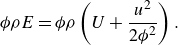 \begin{align} & \phi \rho E= {\phi } \rho \left ( U + {\frac {u^2}{2 {\phi ^2}}} \right ). \end{align}
The species kinetic equations are coupled with the kinetic equations for the mixture through the dependence of mixture internal energy (3.3) on the composition. From (3.1), (3.3) and (3.8), the temperature is evaluated by solving the integral equation,
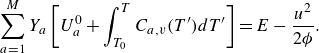 \begin{equation} \sum _{a=1}^MY_a\left [U_a^0 + \int _{T_0}^T {C}_{a,v}(T')dT'\right ]=E-\frac {u^2}{2 {\phi }}. \end{equation}
The temperature evaluated by solving (3.9) enters the species lattice Boltzmann system through the pressure (2.3), forming a two-way coupling.
The lattice Boltzmann equations for the momentum and for the energy lattice are patterned from the single-component developments (Saadat et al. Reference Saadat, Hosseini, Dorschner and Karlin2021) and are realised on the $D3Q27$
discrete velocity set. The mixture lattice Boltzmann equations are written as
$D3Q27$
discrete velocity set. The mixture lattice Boltzmann equations are written as
 \begin{align} f_i(\boldsymbol{x}+\boldsymbol{c}_i \delta t,t+\delta t)- f_i(\boldsymbol{x},t)&= \omega (f_i^{ {ex}} -f_i), \end{align}
 \begin{align} g_i(\boldsymbol{x}+\boldsymbol{c}_i \delta t,t+ \delta t) - g_i(\boldsymbol{x},t)&= \omega _1 (g_i^{ {eq}} -g_i) + (\omega - \omega _1) (g_i^{*} -g_i), \end{align}
where relaxation parameters $\omega$
and
$\omega$
and $\omega _1$
are related to the mixture viscosity and thermal conductivity, and we proceed with specifying the pertinent populations in (3.10) and (3.11).
$\omega _1$
are related to the mixture viscosity and thermal conductivity, and we proceed with specifying the pertinent populations in (3.10) and (3.11).
3.2. Extended equilibrium for the momentum lattice
The extended equilibrium populations $f_i^{ {ex}}$
in (3.10) are specified by the product form (2.14), with the parameters identified as
$f_i^{ {ex}}$
in (3.10) are specified by the product form (2.14), with the parameters identified as ${\xi }_{\alpha }={{u}_{\alpha }^{ {ex}}/\phi }$
and
${\xi }_{\alpha }={{u}_{\alpha }^{ {ex}}/\phi }$
and ${\mathcal{P}}_{\alpha \alpha }={\mathcal{P}}_{\alpha \alpha }^{ {ex}}$
,
${\mathcal{P}}_{\alpha \alpha }={\mathcal{P}}_{\alpha \alpha }^{ {ex}}$
,
 \begin{equation} f_{i}^{ {ex}}= \phi \rho \Psi _{c_{ix}}\left ({\frac {u_{x}^{ {ex}}}{\phi }},{\mathcal{P}}_{xx}^{ {ex}}\right ) \Psi _{c_{iy}}\left ({\frac {u_{y}^{ {ex}}}{\phi }},{\mathcal{P}}_{yy}^{ {ex}}\right ) \Psi _{c_{iz}}\left ({\frac {u_{z}^{ {ex}}}{\phi }},{\mathcal{P}}_{zz}^{ {ex}}\right ), \end{equation}
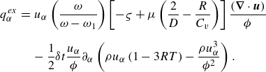
Here, the extended parameter ${\mathcal{P}}_{\alpha \alpha }^{ {ex}}$
reads
${\mathcal{P}}_{\alpha \alpha }^{ {ex}}$
reads
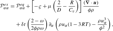 \begin{eqnarray} {\mathcal{P}}_{\alpha \alpha }^{ {ex}} &=& {\mathcal{P}}_{\alpha \alpha }^{ {eq}} + \left [ - \varsigma + \mu \left ( \frac {2}{D} - \frac {R}{C_v} \right ) \right ] \frac {(\boldsymbol{\nabla }\cdot \boldsymbol{u})}{\phi \rho } \nonumber\\[6pt]&& +\, \delta t\left ( \frac {2-\omega }{2 \phi \rho \omega }\right ) \partial _\alpha \left (\rho u_\alpha (1 - 3 R T) - {\frac {\rho u_\alpha ^3}{\phi ^2}}\right ), \end{eqnarray}
where $C_v=\sum _{a=1}^M Y_a C_{a,v}$
is the mixture specific heat at constant volume,
$C_v=\sum _{a=1}^M Y_a C_{a,v}$
is the mixture specific heat at constant volume, $\mu$
is the dynamic viscosity,
$\mu$
is the dynamic viscosity, $\varsigma$
is the bulk viscosity, while
$\varsigma$
is the bulk viscosity, while ${\mathcal{P}}_{\alpha \alpha }^{ {eq}}$
is
${\mathcal{P}}_{\alpha \alpha }^{ {eq}}$
is
 \begin{align} {\mathcal{P}}_{\alpha \alpha }^{ {eq}}& = RT+\frac {u_\alpha ^2}{{\phi ^2}}. \end{align}
Furthermore, the extended velocity $\boldsymbol{u}^{ {ex}}$
in (3.12) takes into account the effect of permeability through the force density due to Knudsen diffusion,
$\boldsymbol{u}^{ {ex}}$
in (3.12) takes into account the effect of permeability through the force density due to Knudsen diffusion, $\boldsymbol{\mathcal{F}}^{ {k}}$
:
$\boldsymbol{\mathcal{F}}^{ {k}}$
:
 \begin{align} u_{\alpha }^{ {ex}}=u_{\alpha } \left ( 1 + \frac {\delta t}{\omega } \frac {1}{\rho } \mathcal{F}_\alpha ^{ {k}} \right ). \end{align}
As it is visible from the second last term in (2.7), the effect of the Knudsen diffusion is to introduce a net retardation on the species which would not vanish once the momentum represented by (2.7) is summed over all the components. This net retardation is provided by the DGM and it allows to introduce exact penalisation to the hydrodynamic mean momentum equation (Angot Reference Angot1999; Hardy et al. Reference Hardy, De Wilde and Winckelmans2019; Sharaborin et al. Reference Sharaborin, Rogozin and Kasimov2021), without a need for free parameters and making it unnecessary to invoke estimates for permeability (Brinkman Reference Brinkman1949). Once obtained from the net momentum loss associated with the last term on the right-hand side of (2.20), the penalisation is introduced through the term $\boldsymbol{\mathcal{F}}^{ {k}}$
, which essentially acts as a correction to the hydrodynamic flux. It is computed as
$\boldsymbol{\mathcal{F}}^{ {k}}$
, which essentially acts as a correction to the hydrodynamic flux. It is computed as
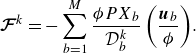 \begin{align} {\boldsymbol{\mathcal{F}}^{ {k}}=-\sum _{b=1}^M \frac {\phi P X_b}{\mathcal{D}_{b}^{ {k}}} \left (\frac {\boldsymbol{u}_{b}}{\phi }\right )}. \end{align}
Finally, the effect of extension featured by the third term in (3.13) is to correct for the incomplete Galilean invariance of the standard $D3Q27$
velocity set (2.10). The second term in (3.13) is necessary to impose the correct bulk viscosity
$D3Q27$
velocity set (2.10). The second term in (3.13) is necessary to impose the correct bulk viscosity $\varsigma$
(Sawant et al. Reference Sawant, Dorschner and Karlin2022). With all the above specifications, the equilibrium pressure tensor
$\varsigma$
(Sawant et al. Reference Sawant, Dorschner and Karlin2022). With all the above specifications, the equilibrium pressure tensor $P_{\alpha \beta }^{ {eq}}$
is found as
$P_{\alpha \beta }^{ {eq}}$
is found as
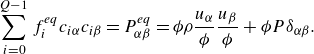 \begin{align} \sum _{i=0}^{Q-1} f_i^{ {eq}} c_{i\alpha } c_{i\beta } = P_{\alpha \beta }^{ {eq}} = \phi \rho \frac {u_\alpha }{ \phi } \frac {u_\beta }{ \phi } + \phi P \delta _{\alpha \beta }. \end{align}
3.3. Equilibrium and quasi-equilibrium of the energy lattice
For the energy lattice, the corresponding equilibrium and quasi-equilibrium populations in (3.11) are evaluated along the lines of Saadat et al. (Reference Saadat, Hosseini, Dorschner and Karlin2021) using linear operators $\mathcal{O}_\alpha$
, acting on any smooth function
$\mathcal{O}_\alpha$
, acting on any smooth function $A(\boldsymbol{u},T)$
according to a rule,
$A(\boldsymbol{u},T)$
according to a rule,
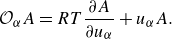 \begin{equation} \mathcal O_\alpha A= RT \frac {\partial A}{\partial u_\alpha } + u_\alpha A. \end{equation}
By substituting the parameters $\xi _\alpha = \mathcal{O}_\alpha$
and
$\xi _\alpha = \mathcal{O}_\alpha$
and ${\mathcal{P}}_{\alpha \alpha } = \mathcal{O}_\alpha ^2$
into the product form (2.14), the equilibrium populations
${\mathcal{P}}_{\alpha \alpha } = \mathcal{O}_\alpha ^2$
into the product form (2.14), the equilibrium populations $g_i^{ {eq}}$
are compactly written using the energy
$g_i^{ {eq}}$
are compactly written using the energy $E$
as the generating function,
$E$
as the generating function,
 \begin{align} g_i^{ {eq}} = \phi \rho \Psi _{c_{ix}}(\mathcal{O}_x,\mathcal{O}_x^2) \Psi _{c_{iy}}(\mathcal{O}_y,\mathcal{O}_y^2) \Psi _{c_{iz}}(\mathcal{O}_z,\mathcal{O}_z^2)E. \end{align}
A direct computation shows that the equilibrium (3.19) satisfies the necessary conditions to recover the mixture energy equation, namely, the equilibrium energy flux $\boldsymbol{q}^{ {eq}}$
and the flux thereof
$\boldsymbol{q}^{ {eq}}$
and the flux thereof $\boldsymbol{R}^{ {eq}}$
,
$\boldsymbol{R}^{ {eq}}$
,
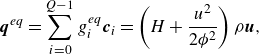 \begin{align} &\boldsymbol{q}^{ {eq}}= \sum _{i=0}^{Q-1} g_i^{ {eq}} \boldsymbol{c}_{i} = \left (H+\frac {u^2}{2 {\phi ^2}}\right )\rho \boldsymbol{u}, \end{align}
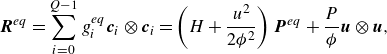 \begin{align} &\boldsymbol{R}^{ {eq}}=\sum _{i=0}^{Q-1} g_i^{ {eq}} \boldsymbol{c}_i\otimes \boldsymbol{c}_i = \left (H+\frac {u^2}{2 {\phi ^2}}\right ) \boldsymbol{P}^{ {eq}} + \frac {P}{ \phi }\boldsymbol{u}\otimes \boldsymbol{u}, \end{align}
where $H$
is the specific mixture enthalpy (3.4). The quasi-equilibrium populations
$H$
is the specific mixture enthalpy (3.4). The quasi-equilibrium populations $g_i^*$
differs from the equilibrium
$g_i^*$
differs from the equilibrium $g_i^{ {eq}}$
by the energy flux only (Karlin et al. Reference Karlin, Sichau and Chikatamarla2013; Saadat et al. Reference Saadat, Hosseini, Dorschner and Karlin2021; Sawant et al. Reference Sawant, Dorschner and Karlin2021),
$g_i^{ {eq}}$
by the energy flux only (Karlin et al. Reference Karlin, Sichau and Chikatamarla2013; Saadat et al. Reference Saadat, Hosseini, Dorschner and Karlin2021; Sawant et al. Reference Sawant, Dorschner and Karlin2021),
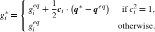 \begin{align} g_{i}^*= \left \{\begin{aligned} & g_{i}^{ {eq}}+\frac {1}{2}\boldsymbol{c}_i\cdot \left (\boldsymbol{q}^*-\boldsymbol{q}^{ {eq}}\right ) &\text{ if } c_i^2=1, & \\ &g_i^{ {eq}} & \text{otherwise}.&\\ \end{aligned}\right . \end{align}
where $\boldsymbol{q}^*$
is a specified quasi-equilibrium energy flux,
$\boldsymbol{q}^*$
is a specified quasi-equilibrium energy flux,
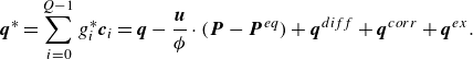 \begin{align} \boldsymbol{q}^{*} &=\sum _{i=0}^{Q-1} g_i^{*} \boldsymbol{c}_{i} = \boldsymbol{q} - \frac {\boldsymbol{u}}{ \phi } \cdot (\boldsymbol{P} - \boldsymbol{P}^{ {eq}}) +\boldsymbol{q}^{ {diff}}+\boldsymbol{q}^{ {corr}}+\boldsymbol{q}^{ {ex}}. \end{align}
The two first terms in (3.23) maintain a variable Prandtl number and include the energy flux $\boldsymbol{q}$
and the pressure tensor
$\boldsymbol{q}$
and the pressure tensor $\boldsymbol{P}$
,
$\boldsymbol{P}$
,
 \begin{align} & \boldsymbol{q}=\sum _{i=0}^{Q-1} g_i \boldsymbol{c}_{i}, \end{align}
 \begin{align} & \boldsymbol{P}=\sum _{i=0}^{Q-1} f_i \boldsymbol{c}_{i}\otimes \boldsymbol{c}_{i}. \end{align}
The interdiffusion energy flux $\boldsymbol{q}^{ {diff}}$
,
$\boldsymbol{q}^{ {diff}}$
,
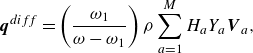 \begin{align} \boldsymbol{q}^{ {diff}} =\left (\frac {\omega _1}{\omega -\omega _1} \right ) \rho \sum _{a=1}^{M}H_aY_a \boldsymbol{V}_a, \end{align}
where the diffusion velocities $\boldsymbol{V}_a$
are defined by (2.29), contributes the enthalpy transport due to diffusion, cf. Sawant et al. (Reference Sawant, Dorschner and Karlin2021). Moreover, the correction flux
$\boldsymbol{V}_a$
are defined by (2.29), contributes the enthalpy transport due to diffusion, cf. Sawant et al. (Reference Sawant, Dorschner and Karlin2021). Moreover, the correction flux $\boldsymbol{q}^{ {corr}}$
is required in the two-population approach to the mixtures to recover the Fourier law of thermal conduction (Sawant et al. Reference Sawant, Dorschner and Karlin2021),
$\boldsymbol{q}^{ {corr}}$
is required in the two-population approach to the mixtures to recover the Fourier law of thermal conduction (Sawant et al. Reference Sawant, Dorschner and Karlin2021),
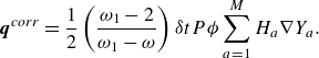 \begin{align} \boldsymbol{q}^{ {corr}}=\frac {1}{2}\left (\frac {\omega _1-2}{\omega _1-\omega }\right ) {\delta t}P \phi \sum _{a=1}^M H_{a} \nabla Y_a. \end{align}
The term $\boldsymbol{q}^{ {ex}}$
in the quasi-equilibrium flux (3.23) is required for consistency with the extended equilibrium (3.12). Components of the vector
$\boldsymbol{q}^{ {ex}}$
in the quasi-equilibrium flux (3.23) is required for consistency with the extended equilibrium (3.12). Components of the vector $\boldsymbol{q}^{ {ex}}$
follow the structure of (3.13),
$\boldsymbol{q}^{ {ex}}$
follow the structure of (3.13),
 \begin{eqnarray} {q}_\alpha ^{ {ex}} &=& u_\alpha \left ( \frac {\omega }{\omega -\omega _1} \right ) \left [ - \varsigma + \mu \left ( \frac {2}{D} - \frac {R}{C_v} \right ) \right ] \frac {(\boldsymbol{\nabla }\cdot \boldsymbol{u})}{\phi } \nonumber\\[6pt]&& -\, \frac {1}{2}\delta t \frac {u_\alpha }{\phi } \partial _\alpha \left (\rho u_\alpha \left (1 - 3 R T\right ) - \frac {\rho u_\alpha ^3}{{\phi ^2}} \right ). \end{eqnarray}
Spatial derivatives in the correction flux (3.27) and in the isotropy correction (3.13) and (3.28) were implemented using isotropic lattice operators (Thampi et al. Reference Thampi, Ansumali, Adhikari and Succi2013).
In summary, the lattice Boltzmann model for an $M$
-component mixture of ideal gases on the standard
$M$
-component mixture of ideal gases on the standard $D3Q27$
lattice consists of
$D3Q27$
lattice consists of $M$
species lattices where the lattice Boltzmann equation is given by (2.21), and the momentum and energy lattice Boltzmann equations (3.10) and (3.11). In total, the
$M$
species lattices where the lattice Boltzmann equation is given by (2.21), and the momentum and energy lattice Boltzmann equations (3.10) and (3.11). In total, the $M+2$
lattice Boltzmann equations are tightly coupled, as has been already specified above: The temperature from the energy lattice is provided to the species lattices through species equilibrium (2.15) and quasi-equilibrium (2.16), (2.17) and (2.18), but also in the Stefan–Maxwell temperature-dependent relaxation rates (2.23) and the Knudsen diffusion temperature-dependent relaxation rates (2.26).
$M+2$
lattice Boltzmann equations are tightly coupled, as has been already specified above: The temperature from the energy lattice is provided to the species lattices through species equilibrium (2.15) and quasi-equilibrium (2.16), (2.17) and (2.18), but also in the Stefan–Maxwell temperature-dependent relaxation rates (2.23) and the Knudsen diffusion temperature-dependent relaxation rates (2.26).
Looking at the information flowing in the other direction, the net force due to Knudsen diffusion $\boldsymbol{\mathcal{F}}^{ {k}}$
(3.16) is an input to the momentum lattice which relies on the component velocity and composition from the species lattices. The species diffusion velocities serve also as input to the quasi-equilibrium population of the energy lattice via the interdiffusion flux (3.26). The mass fractions from the species lattices are used to compute the mixture energy (3.3) and enthalpy (3.4) in the equilibrium and the quasi-equilibrium of the momentum and energy lattices. The momentum and the energy lattices remain coupled in the standard way already present in the single-component setting. In the present formulation, we use the interconnections between the species, and the momentum and energy lattices, which has been termed as weak coupling by Sawant et al. (Reference Sawant, Dorschner and Karlin2022). It should be noted that the other, stronger forms of coupling mentioned by Sawant et al. (Reference Sawant, Dorschner and Karlin2022) cannot be used with the present formulation. This happens because the stronger forms of coupling described by Sawant et al. (Reference Sawant, Dorschner and Karlin2022) eliminate the momentum of one of the species, which would then lead to incorrect net force
$\boldsymbol{\mathcal{F}}^{ {k}}$
(3.16) is an input to the momentum lattice which relies on the component velocity and composition from the species lattices. The species diffusion velocities serve also as input to the quasi-equilibrium population of the energy lattice via the interdiffusion flux (3.26). The mass fractions from the species lattices are used to compute the mixture energy (3.3) and enthalpy (3.4) in the equilibrium and the quasi-equilibrium of the momentum and energy lattices. The momentum and the energy lattices remain coupled in the standard way already present in the single-component setting. In the present formulation, we use the interconnections between the species, and the momentum and energy lattices, which has been termed as weak coupling by Sawant et al. (Reference Sawant, Dorschner and Karlin2022). It should be noted that the other, stronger forms of coupling mentioned by Sawant et al. (Reference Sawant, Dorschner and Karlin2022) cannot be used with the present formulation. This happens because the stronger forms of coupling described by Sawant et al. (Reference Sawant, Dorschner and Karlin2022) eliminate the momentum of one of the species, which would then lead to incorrect net force $\boldsymbol{\mathcal{F}}^{ {k}}$
.
$\boldsymbol{\mathcal{F}}^{ {k}}$
.
3.4. Mixture mass, momentum and energy equations
With the equilibrium and quasi-equilibrium populations specified, the hydrodynamic limit of the two-population lattice Boltzmann system (3.10) and (3.11) is found by expanding the propagation to second order in the time step $\delta t$
and evaluating the moments of the resulting expansion. Details of the analysis are presented in the Appendix. The continuity equation (Whitaker Reference Whitaker1999), the momentum equation with penalisation (Whitaker Reference Whitaker1999; Liu & Vasilyev Reference Liu and Vasilyev2007; Fuchsberger et al. Reference Fuchsberger, Aigner, Niederer, Plank, Schima, Haase and Karabelas2022) and the energy equations for a reactive multicomponent mixture (Williams Reference Williams1985; Bird et al. Reference Bird, Stewart and Lightfoot2007; Kee et al. Reference Kee, Coltrin, Glarborg and Zhu2017) are respectively
$\delta t$
and evaluating the moments of the resulting expansion. Details of the analysis are presented in the Appendix. The continuity equation (Whitaker Reference Whitaker1999), the momentum equation with penalisation (Whitaker Reference Whitaker1999; Liu & Vasilyev Reference Liu and Vasilyev2007; Fuchsberger et al. Reference Fuchsberger, Aigner, Niederer, Plank, Schima, Haase and Karabelas2022) and the energy equations for a reactive multicomponent mixture (Williams Reference Williams1985; Bird et al. Reference Bird, Stewart and Lightfoot2007; Kee et al. Reference Kee, Coltrin, Glarborg and Zhu2017) are respectively
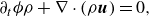 \begin{align} &\partial _t \phi \rho + \nabla \cdot (\rho \boldsymbol{u})=0, \end{align}
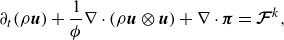 \begin{align} &\partial _t (\rho \boldsymbol{u}) + \frac {1}{ \phi } \nabla \cdot ({\rho \boldsymbol{u}\otimes \boldsymbol{u} })+ \nabla \cdot \boldsymbol{\pi }=\boldsymbol{\mathcal{F}}^{ {k}}, \end{align}
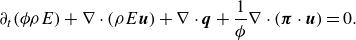 \begin{align} &\partial _t ( \phi \rho E)+\nabla \cdot (\rho E\boldsymbol{u})+ \nabla \cdot \boldsymbol{q}+ \frac {1}{ \phi } \nabla \cdot (\boldsymbol{\pi }\cdot \boldsymbol{u})=0. \end{align}
Here, the pressure tensor $\boldsymbol{\pi }$
in the momentum equation reads
$\boldsymbol{\pi }$
in the momentum equation reads
 \begin{equation} \boldsymbol{\pi }= \phi P\boldsymbol{I} -\mu \left ( \nabla \boldsymbol{u} + \nabla \boldsymbol{u}^{\dagger } -\frac {2}{D} (\nabla \cdot \boldsymbol{u})\boldsymbol{I} \right ) -\varsigma (\nabla \cdot \boldsymbol{u}) \boldsymbol{I}, \end{equation}
where the dynamic viscosity $\mu$
is related to the relaxation parameter
$\mu$
is related to the relaxation parameter $\omega$
,
$\omega$
,
 \begin{align} \mu &= \left ( \frac {1}{\omega } - \frac {1}{2}\right ) P{\delta t}. \end{align}
Note that, in the present lattice Boltzmann formulation, the bulk viscosity $\varsigma$
is a tuneable parameter, cf. Sawant et al. (Reference Sawant, Dorschner and Karlin2022). The heat flux
$\varsigma$
is a tuneable parameter, cf. Sawant et al. (Reference Sawant, Dorschner and Karlin2022). The heat flux $\boldsymbol{q}$
in the energy equation (3.31) reads
$\boldsymbol{q}$
in the energy equation (3.31) reads
 \begin{equation} \boldsymbol{q}=- \phi \lambda \nabla T+\rho \sum _{a=1}^{M}H_aY_a {\boldsymbol{V}_a} . \end{equation}
The first term in (3.34) is the Fourier law of thermal conduction in the gas phase (Kee et al. Reference Kee, Coltrin, Glarborg and Zhu2017), with thermal conductivity $\lambda$
related to the relaxation parameter
$\lambda$
related to the relaxation parameter $\omega _1$
,
$\omega _1$
,
 \begin{equation} \lambda = \left (\frac {1}{\omega _1} - \frac {1}{2}\right ) P C_p{\delta t}, \end{equation}
where $C_p=C_v+R$
is the mixture specific heat at constant pressure. The second term in (3.34) is the interdiffusion energy flux. With the thermal diffusivity
$C_p=C_v+R$
is the mixture specific heat at constant pressure. The second term in (3.34) is the interdiffusion energy flux. With the thermal diffusivity $\alpha =\lambda /\rho C_p$
and the kinematic viscosity
$\alpha =\lambda /\rho C_p$
and the kinematic viscosity $\nu =\mu /\rho$
, the Prandtl number becomes
$\nu =\mu /\rho$
, the Prandtl number becomes ${\textrm {Pr}} = {\nu }/{\alpha }$
. For the present reactive flow formulation, the local dynamic viscosity
${\textrm {Pr}} = {\nu }/{\alpha }$
. For the present reactive flow formulation, the local dynamic viscosity $\mu (\boldsymbol{x},t)$
and the thermal conductivity
$\mu (\boldsymbol{x},t)$
and the thermal conductivity $\lambda (\boldsymbol{x},t)$
of the mixture are evaluated as a function of the local chemical state by using the chemical kinetics solver Cantera (Wilke Reference Wilke1950; Mathur et al. Reference Mathur, Tondon and Saxena1967; Kee et al. Reference Kee, Coltrin and Glarborg2003; Goodwin et al. Reference Goodwin, Moffat, Schoegl, Speth and Weber2018).
$\lambda (\boldsymbol{x},t)$
of the mixture are evaluated as a function of the local chemical state by using the chemical kinetics solver Cantera (Wilke Reference Wilke1950; Mathur et al. Reference Mathur, Tondon and Saxena1967; Kee et al. Reference Kee, Coltrin and Glarborg2003; Goodwin et al. Reference Goodwin, Moffat, Schoegl, Speth and Weber2018).
4. Reactions in porous electrodes
To get useful insights from applying the model developed so far to reactive flow in porous electrodes, the model needs to be augmented with some additions pertaining to electrochemical reactions. Source terms need to be introduced into the kinetic equation for energy (3.11) to account for ohmic heat, energy lost as electricity and for balancing the energy changes due to interchange of species between the surface phase and the bulk phase. The kinetic equation for momentum (3.10) also needs to account for the change of mass caused by adsorption and desorption.
Within a representative elementary volume, let us define $a^{ {(s)}}_k$
as the specific surface area of a reactive surface
$a^{ {(s)}}_k$
as the specific surface area of a reactive surface $k$
. The specific surface area is the area available for surface reactions per unit volume of the porous material (Kee et al. Reference Kee, Coltrin, Glarborg and Zhu2017). The product of specific surface area and the surface rate of production of species gives the bulk production rate of the species. For a gas phase species with the density
$k$
. The specific surface area is the area available for surface reactions per unit volume of the porous material (Kee et al. Reference Kee, Coltrin, Glarborg and Zhu2017). The product of specific surface area and the surface rate of production of species gives the bulk production rate of the species. For a gas phase species with the density $\rho _a$
, its total mass production rate per unit volume in the gas phase
$\rho _a$
, its total mass production rate per unit volume in the gas phase $\dot \rho _a^{({f})}$
is computed as (DeCaluwe et al. Reference DeCaluwe, Zhu, Kee and Jackson2008)
$\dot \rho _a^{({f})}$
is computed as (DeCaluwe et al. Reference DeCaluwe, Zhu, Kee and Jackson2008)
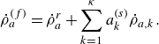 \begin{align} \dot \rho _a^{({f})} = \dot \rho _a^{ {r}} + \sum _{k=1}^\kappa a^{ {(s)}}_k \dot \rho _{a,k} . \end{align}
In (4.1), $\dot \rho _a^{ {r}}$
is the net mass production rate per unit volume of species
$\dot \rho _a^{ {r}}$
is the net mass production rate per unit volume of species $a$
in the fluid phase due to homogeneous reactions and
$a$
in the fluid phase due to homogeneous reactions and $\dot \rho _{a,k}$
is the net mass production rate of species
$\dot \rho _{a,k}$
is the net mass production rate of species $a$
due to heterogeneous reactions per unit surface area of the surface
$a$
due to heterogeneous reactions per unit surface area of the surface $k$
, out of the
$k$
, out of the $\kappa$
number of chemically active surfaces. The latter is calculated as
$\kappa$
number of chemically active surfaces. The latter is calculated as
 \begin{align} \dot \rho _{a,k} = m_a \dot M_{a,k}^{({f})}, \end{align}
with $\dot M_{a,k}^{({f})}$
being the molar production rate of the fluid phase species
$\dot M_{a,k}^{({f})}$
being the molar production rate of the fluid phase species $a$
per unit surface area of the surface material
$a$
per unit surface area of the surface material $k$
. The molar production rate
$k$
. The molar production rate $\dot M_{a,k}^{({f})}$
is responsible for describing interchange between the aforementioned fluid phase species
$\dot M_{a,k}^{({f})}$
is responsible for describing interchange between the aforementioned fluid phase species $a$
and the surface phase species that exist on the surface in an adsorbed state. The composition of the surface species is described by the number of moles per unit area of the adsorbed site
$a$
and the surface phase species that exist on the surface in an adsorbed state. The composition of the surface species is described by the number of moles per unit area of the adsorbed site $M_{a,k}^{ {(s)}}$
and the constant site density
$M_{a,k}^{ {(s)}}$
and the constant site density $\Gamma _k$
, which is the total capacity of the surface to host adsorbed species. The mole fraction of an adsorbed species is then defined as
$\Gamma _k$
, which is the total capacity of the surface to host adsorbed species. The mole fraction of an adsorbed species is then defined as
 \begin{align} X_{a,k}^{ {(s)}} = \frac {M_{a,k}^{ {(s)}}}{\Gamma _k}. \end{align}
Analogous to the surface reactions, the edges formed at the intersection of the surfaces are also capable of hosting chemical reactions. The edges are described by their specific length $l^{ {(e)}}_p$
, i.e. the length of the edge
$l^{ {(e)}}_p$
, i.e. the length of the edge $p$
per unit volume of the REV. The net reaction rate of a surface species
$p$
per unit volume of the REV. The net reaction rate of a surface species $a$
on an edge
$a$
on an edge $p$
are then described by the molar production rate per unit length
$p$
are then described by the molar production rate per unit length $\dot M_{a,p}^{ {(e)}}$
. The rate of change of a surface species
$\dot M_{a,p}^{ {(e)}}$
. The rate of change of a surface species $a$
residing on the surface
$a$
residing on the surface $k$
is the non-dimensionalised sum of its molar production rate on the surface
$k$
is the non-dimensionalised sum of its molar production rate on the surface $k$
and its molar production rate on all the edges
$k$
and its molar production rate on all the edges $p$
belonging to the surface
$p$
belonging to the surface $k$
. Mathematically, the rate of change of mole fraction
$k$
. Mathematically, the rate of change of mole fraction $\dot X_{a,k}^{ {(s)}}$
is written as (DeCaluwe et al. Reference DeCaluwe, Zhu, Kee and Jackson2008)
$\dot X_{a,k}^{ {(s)}}$
is written as (DeCaluwe et al. Reference DeCaluwe, Zhu, Kee and Jackson2008)
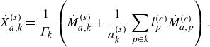 \begin{align} \dot X_{a,k}^{ {(s)}} = \frac {1}{\Gamma _k} \left ( \dot M_{a,k}^{ {(s)}} + \frac {1}{a^{ {(s)}}_k} \sum _{p \in k} l^{ {(e)}}_p \dot M_{a,p}^{ {(e)}} \right ). \end{align}
In this work, we solve for the flow through porous electrodes which are made up of spherical microstructures of at most two substances. The anode is made of nickel and yttria-stabilised zirconia (YSZ), while the cathode is made up of lanthanum strontium manganite (LSM) and YSZ. The nickel and the LSM form the electrode phase in the anode and the cathode, respectively. The YSZ forms the electrolyte phase in both the anode and the cathode. The intersection of the micro spheres of the electrode and the electrolyte phase form an edge, which is also referred to as the TPB in the literature (Zhao & Virkar Reference Zhao and Virkar2005). The TPB is the site of intersection of the electrode, the electrolyte and the gas phase. In this work, we use the mass action kinetics detailed chemistry model proposed by DeCaluwe et al. (Reference DeCaluwe, Zhu, Kee and Jackson2008). In this model, the adsorption is modelled though the gas–electrode surface reactions and the gas–electrolyte surface reactions. There is only one edge phase, which represents the TPB. The edge reactions involve only the adsorbed surface phase species. The rate equation (4.4) simplifies to
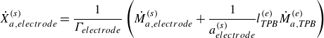 \begin{align} \dot X_{a, {electrode}}^{ {(s)}} = \frac {1}{\Gamma _{ {electrode}}} \left ( \dot M_{a, {electrode}}^{ {(s)}} + \frac {1}{a^{ {(s)}}_{ {electrode}}} l^{ {(e)}}_{ {T\!P\!B}} \dot M_{a,{T\!P\!B}}^{ {(e)}} \right ) \end{align}
for the species adsorbed on the electrode material surface and
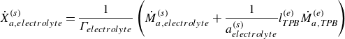 \begin{align} \dot X_{a,{electrolyte}}^{ {(s)}} = \frac {1}{\Gamma _{ {electrolyte}}} \left ( \dot M_{a,{electrolyte}}^{ {(s)}} + \frac {1}{a^{ {(s)}}_{ {electrolyte}}} l^{ {(e)}}_{ {T\!P\!B}} \dot M_{a,{T\!P\!B}}^{ {(e)}} \right ) \end{align}
for the species adsorbed on the electrolyte material surface.
The oxidation reactions in the anode and the reduction reactions in the cathode are defined to occur in the TPB. Consequently, the electron production rates are a function of the composition of the adsorbed species on their respective surfaces as well as the potential $\Phi$
in the bulk electrolyte and the bulk electrode phase. The electric current is obtained as a product of Faraday’s constant
$\Phi$
in the bulk electrolyte and the bulk electrode phase. The electric current is obtained as a product of Faraday’s constant $ F$
and the molar production rate of the electrons
$ F$
and the molar production rate of the electrons $\dot M_{ {electron},{T\!P\!B}}^{ {(s)}}$
. The volumetric current density
$\dot M_{ {electron},{T\!P\!B}}^{ {(s)}}$
. The volumetric current density $\mathcal{I}^{ {(v)}}$
, which is the current generated per unit volume of the REV, is calculated as
$\mathcal{I}^{ {(v)}}$
, which is the current generated per unit volume of the REV, is calculated as
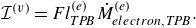 \begin{align} \mathcal{I}^{ {(v)}} = F l^{ {(e)}}_{ {T\!P\!B}} \dot M_{ {electron},{T\!P\!B}}^{ {(e)}}. \end{align}
A positive $\mathcal{I}^{ {(v)}}$
indicates production of electrons, which is a result of oxidation, while a negative
$\mathcal{I}^{ {(v)}}$
indicates production of electrons, which is a result of oxidation, while a negative $\mathcal{I}^{ {(v)}}$
is a consequence of the loss of electrons due to a reduction reaction.
$\mathcal{I}^{ {(v)}}$
is a consequence of the loss of electrons due to a reduction reaction.
4.1. Charge transport
The simplest SOFC membrane electrode assembly (MEA) consists of three major sections, as skeched in figure 1. A porous composite anode section made of nickel and YSZ, an impervious solid electrolyte section consisting only of YSZ, and a porous composite cathode section made up of LSM and YSZ (Bove & Ubertini Reference Bove and Ubertini2006). To model charge transport in the cell, we follow the model proposed by Bessler et al. (Reference Bessler, Gewies and Vogler2007b
). The equations therein are reproduced in this section for completeness. A typical MEA consists of thin layers of the three sections sandwiched together. We model the charge transport by only considering the gradients in a direction $x$
, which is normal to the interface between these layers. We also colloquially refer to this direction to be along the length of the MEA.
$x$
, which is normal to the interface between these layers. We also colloquially refer to this direction to be along the length of the MEA.
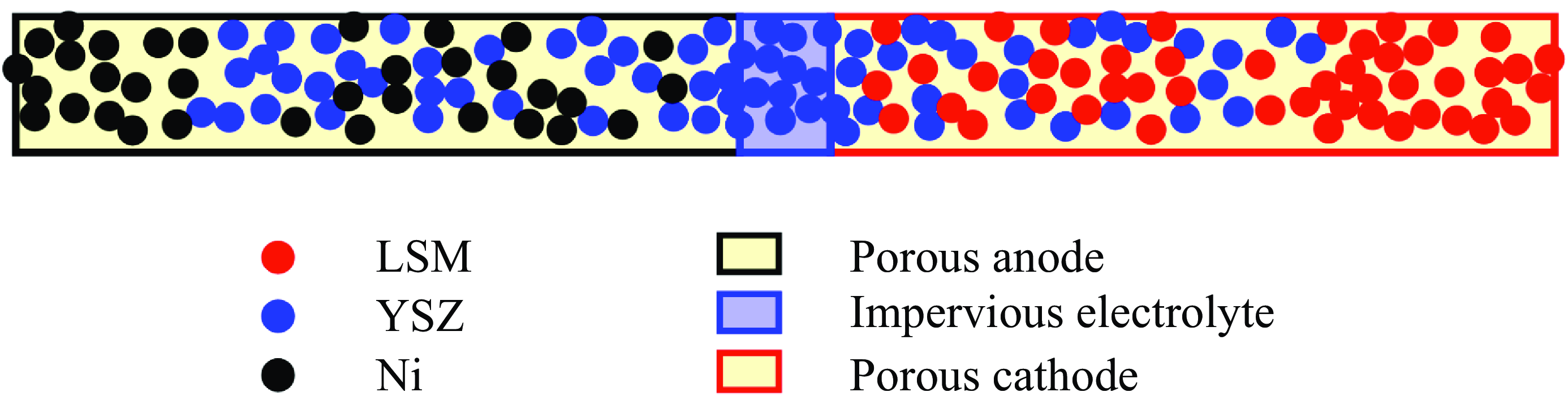
Figure 1. Sketch of a 1-D SOFC.
Since the electrode phase has a high electron conductivity as compared with the electrolyte phase, the electrode phase is assumed to have a spatially constant electric potential, i.e.
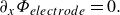 \begin{align} \partial _x \Phi _{ {electrode}} = 0. \end{align}
However, the electrolyte phase has a finite ion conductivity. The current density per unit area $\,\mathcal{I}^{ {(a)}}$
is obtained by integrating the volumetric current density over and along the length of the MEA,
$\,\mathcal{I}^{ {(a)}}$
is obtained by integrating the volumetric current density over and along the length of the MEA,
 \begin{align} \mathcal{I}^{ {(a)}}(x) = \int \mathcal{I}^{ {(v)}}(x) {\rm d}x. \end{align}
Function $\mathcal{I}^{ {(a)}}$
is often concisely referred to as the current density in the literature. By Ohm’s law, the potential in the electrolyte phase
$\mathcal{I}^{ {(a)}}$
is often concisely referred to as the current density in the literature. By Ohm’s law, the potential in the electrolyte phase $\Phi _{ {electrolyte}}$
is obtained by integrating the product of resistivity of the electrolyte phase
$\Phi _{ {electrolyte}}$
is obtained by integrating the product of resistivity of the electrolyte phase $\Omega _{ {electrolyte}}$
and the current density,
$\Omega _{ {electrolyte}}$
and the current density,
 \begin{align} \Phi _{ {electrolyte}} (x) = \int \mathcal{I}^{ {(a)}}(x) \; \Omega _{ {electrolyte}}(x) {\rm d}x. \end{align}
The resistivity of the electrolyte phase is a function of space, owing to the different composition of the MEA components.
In the simulations, we set a certain potential difference on the anode side of the cell, $\Delta \Phi _{ {anode}} = \Phi _{ {Ni}} - \Phi _{ {YSZ}}$
. The potential
$\Delta \Phi _{ {anode}} = \Phi _{ {Ni}} - \Phi _{ {YSZ}}$
. The potential $\Phi _{ {YSZ}}$
is chosen to be zero at the beginning of the electrochemically active section of the anode. This potential difference, along with the local composition of adsorbed species and the temperature, produces a certain volumetric current density described by (4.7). The volumetric current density in the sandwiched solid electrolyte section is vanishing. Next, we integrate the volumetric current density with (4.9) to obtain the current density
$\Phi _{ {YSZ}}$
is chosen to be zero at the beginning of the electrochemically active section of the anode. This potential difference, along with the local composition of adsorbed species and the temperature, produces a certain volumetric current density described by (4.7). The volumetric current density in the sandwiched solid electrolyte section is vanishing. Next, we integrate the volumetric current density with (4.9) to obtain the current density $\mathcal{I}^{ {(a)}}(x)$
and simultaneously integrate the current density with (4.10) to obtain the electrolyte potential throughout the length of the active electrolyte phase. Once the current density and the electrolyte potential up to the electrolyte–cathode interface becomes known by integration, the cathode electrode potential
$\mathcal{I}^{ {(a)}}(x)$
and simultaneously integrate the current density with (4.10) to obtain the electrolyte potential throughout the length of the active electrolyte phase. Once the current density and the electrolyte potential up to the electrolyte–cathode interface becomes known by integration, the cathode electrode potential $\Phi _{ {LSM}}$
is determined by solving (4.7) in a reverse manner. In other words, the potential difference
$\Phi _{ {LSM}}$
is determined by solving (4.7) in a reverse manner. In other words, the potential difference $\Delta \Phi _{ {cathode}} = \Phi _{ {LSM}} - \Phi _{ {YSZ}}$
is varied by iterating
$\Delta \Phi _{ {cathode}} = \Phi _{ {LSM}} - \Phi _{ {YSZ}}$
is varied by iterating $\Phi _{ {LSM}}$
with the Secant method until the target current density matches the same value as that at the anode is obtained. The cell voltage is then found as
$\Phi _{ {LSM}}$
with the Secant method until the target current density matches the same value as that at the anode is obtained. The cell voltage is then found as $\Phi _{ {cell}} = \Phi _{ {LSM}} - \Phi _{ {Ni}}$
.
$\Phi _{ {cell}} = \Phi _{ {LSM}} - \Phi _{ {Ni}}$
.
4.2. Source terms in the hydrodynamics equations
As defined by (4.1), when the mass production rate $\dot \rho _a^{({f})}$
includes the production rates due to adsorption and desorption reactions, the total post-collision fluid density of the mixture
$\dot \rho _a^{({f})}$
includes the production rates due to adsorption and desorption reactions, the total post-collision fluid density of the mixture $\rho ^{ (pc)}$
changes from the density of the mixture before the species collision step (2.21) is executed. From the nature of the reaction term (2.32), the change in fluid density can be computed by summing over the mass production rates,
$\rho ^{ (pc)}$
changes from the density of the mixture before the species collision step (2.21) is executed. From the nature of the reaction term (2.32), the change in fluid density can be computed by summing over the mass production rates,
 \begin{eqnarray} \phi \rho ^{ (pc)} &=& \phi \sum _{a=1}^M \rho _a + \sum _{a=1}^M \dot \rho _a^{({f})} \delta t \nonumber\\[6pt] &=& \phi \sum _{a=1}^M \rho _a + \sum _{a=1}^M \left ( \dot \rho _a^{ {r}} + \sum _{k=1}^\kappa a^{ {(s)}}_k \dot \rho _{a,k} \right ) \delta t \nonumber\\[6pt] &=& \phi \rho + \sum _{a=1}^M \sum _{k=1}^\kappa a^{ {(s)}}_k \dot \rho _{a,k} \delta t. \end{eqnarray}
The new density $\rho ^{ (pc)}$
is recorded by the species system of equations (2.21) due to the presence of the source terms. However, due to the reduced description of the model, the kinetic equations for the momentum (3.10) need to be informed about this change. Analogous to the change in density, there are also implications for the energy tracked by (3.11) and which we consider in this section.
$\rho ^{ (pc)}$
is recorded by the species system of equations (2.21) due to the presence of the source terms. However, due to the reduced description of the model, the kinetic equations for the momentum (3.10) need to be informed about this change. Analogous to the change in density, there are also implications for the energy tracked by (3.11) and which we consider in this section.
In this work, we assume that the adsorbed species and the fluid phase species are in thermal equilibrium. Therefore, a ‘unified’ internal energy $\tilde U$
can be defined in a REV as a sum of internal energies of both the fluid state species and the adsorbed species. If there exist
$\tilde U$
can be defined in a REV as a sum of internal energies of both the fluid state species and the adsorbed species. If there exist $M$
fluid state species,
$M$
fluid state species, $B$
adsorbed species on the electrolyte surface and
$B$
adsorbed species on the electrolyte surface and $D$
adsorbed species on the electrode surface, the unified internal energy at temperature
$D$
adsorbed species on the electrode surface, the unified internal energy at temperature $T$
is given by
$T$
is given by
 \begin{eqnarray} \tilde U &=& \phi \rho \sum _{a=1}^MY_a\left [U_a^0 + \int _{T_0}^T {C}_{a,v}(T'){\rm d}T'\right ] \nonumber\\[6pt] && +\, a^{ {(s)}}_{ {electrolyte}} \rho ^{ {(s)}}_{ {electrolyte}} \sum _{b=1}^B Y_b\left [U_b^0 + \int _{T_0}^T {C}_{b,v}(T'){\rm d}T'\right ] \nonumber\\[6pt] && +\, a^{ (s)}_{ {electrode}} \rho ^{ (s)}_{ {electrode}} \sum _{d=1}^D Y_d\left [U_d^0 + \int _{T_0}^T {C}_{d,v}(T'){\rm d}T'\right ]. \end{eqnarray}
Electric power produced due to the production of electrons is lost from the hydrodynamic system (Kee et al. Reference Kee, Coltrin, Glarborg and Zhu2017). This electric power can be calculated based on the local volumetric current as
 \begin{align} \tilde P_{ {elec}} = \lvert \Phi _{ {electrode}} - \Phi _{ {electrolyte}} \rvert \; \mathcal{I}^{ {(v)}}. \end{align}
The resistance of the electrolyte phase to the flow of electrons leads to heating of the hydrodynamic system. This ohmic heat rate is given by
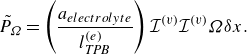 \begin{align} \tilde P_\Omega = \left ( \frac {a_{ {electrolyte}}}{ l^{ {(e)}}_{ {T\!P\!B}} } \right ) \mathcal{I}^{ {(v)}} \mathcal{I}^{ {(v)}} \Omega \delta x. \end{align}
The net effect of the energy loss due to electrical work and the energy gained due to the electrolyte phase resistance is combined into an energy source term $\tilde U_{ {source}}$
,
$\tilde U_{ {source}}$
,
 \begin{align} \tilde U_{ {source}} = ( - \tilde P_\Omega + \tilde P_{ {elec}} ) \delta t. \end{align}
Therefore, the unified internal energy after the species collision step is
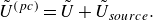 \begin{align} \tilde U^{({pc})} = \tilde U + \tilde U_{ {source}}. \end{align}
After the collision step, we need to know the post-collision internal energy $\rho U^{({pc})}$
of the fluid state, since the kinetic equations only track the evolution of the bulk fluid phase. The post-collision internal energy is found by simple arithmetic manipulation of subtracting the post-collision energy of the adsorbed phases from the post-collision unified internal energy,
$\rho U^{({pc})}$
of the fluid state, since the kinetic equations only track the evolution of the bulk fluid phase. The post-collision internal energy is found by simple arithmetic manipulation of subtracting the post-collision energy of the adsorbed phases from the post-collision unified internal energy,
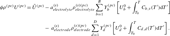 \begin{align} \phi \rho ^{ (pc)} U^{ (pc)} = \tilde U^{ (pc)} & - a^{ {(s)}}_{ {electrolyte}} \rho ^{ {(s)}({pc})}_{ {electrolyte}} \sum _{b=1}^B Y_b^{({pc})} \left [U_b^0 + \int _{T_0}^{T} {C}_{b,v}(T'){\rm d}T'\right ] \nonumber \\[4pt] & -\, a^{ {(s)}}_{ {electrode}} \rho ^{ {(s)}({pc})}_{ {electrode}} \sum _{d=1}^D Y_d^{ {(pc)}} \left [U_d^0 + \int _{T_0}^{T} {C}_{d,d}(T'){\rm d}T'\right ]. \end{align}
Analogous to (3.7), a distribution $g_i^{ {eq}, source}$
is created to account for the change in internal energy. The zeroth moment of these energy source populations represents the new internal energy
$g_i^{ {eq}, source}$
is created to account for the change in internal energy. The zeroth moment of these energy source populations represents the new internal energy $U^{ {(pc)}}$
,
$U^{ {(pc)}}$
,
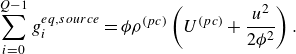 \begin{align} & \sum _{i=0}^{Q-1} g_i^{ {eq}, source} = \phi \rho ^{ {(pc)}} \left ( U^{ {(pc)}} + {\frac {u^2}{2 {\phi ^2}}} \right ). \end{align}
Finally, the kinetic equations (3.10) and (3.11) are modified to account for the mass and energy changes,
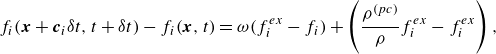 \begin{align} f_i(\boldsymbol{x}+\boldsymbol{c}_i \delta t,t+\delta t)- f_i(\boldsymbol{x},t)&= \omega (f_i^{ {ex}} -f_i) + \left ( \frac {\rho ^{ {(pc)}}}{\rho } f_i^{ {ex}} - f_i^{ {ex}} \right ), \end{align}
 \begin{align} g_i(\boldsymbol{x}+\boldsymbol{c}_i \delta t,t+ \delta t) - g_i(\boldsymbol{x},t)&= \omega _1 (g_i^{ {eq}} -g_i) + (\omega - \omega _1) (g_i^{*} -g_i) + (g_i^{ {eq},source}-g_i^{ {eq}})._{_{_{_{\!}}}} \end{align}
Kinetic equations for the species (2.21) already include populations $\dot f_{ai}^{ {r}}$
for mass production sources through (2.32). In the case of both homogeneous and heterogeneous reactions, these populations are computed with the total mass production rate
$\dot f_{ai}^{ {r}}$
for mass production sources through (2.32). In the case of both homogeneous and heterogeneous reactions, these populations are computed with the total mass production rate $\dot \rho _a^{({f})}$
,
$\dot \rho _a^{({f})}$
,
 \begin{align} \dot f_{ai}^{ {r}} &= \dot \rho _a^{({f})} \Psi _{c_{ix}}\left (\frac {u_{x}}{{\phi }},\frac {u_{x}^2}{{{\phi ^2}}}+R_aT\right ) \Psi _{c_{iy}}\left (\frac {u_{y}}{{\phi }},\frac {u_{y}^2}{{\phi ^2}}+R_aT\right ) \Psi _{c_{iz}}\left (\frac {u_{z}}{{\phi }},\frac {u_{z}^2}{{\phi ^2}}+R_aT\right ). \end{align}
5. Validation
In §§ 2 and 3, a lattice Boltzmann model has been formulated for multicomponent hydrodynamics in porous media. The present formulation replicates the DGM at the macroscopic scale. To numerically validate the model, in the present section, we evaluate the component diffusion fluxes in a ternary mixture undergoing counter-diffusion through a capillary tube. In § 4, the lattice Boltzmann model was extended to include heterogeneous reactions and electrochemistry. This further development shall be validated by comparing the polarisation curves of an SOFC against LBM simulation of a membrane electrode assembly consisting of porous composite electrodes.
Note that the model formulated in this work has been realised on the standard $D3Q27$
lattice, which makes it readily usable for complex three-dimensional set-ups. The model can be used to compute realistic geometries such as porous combustors or geological flows through porous rocks where the geometrical symmetry or lack thereof prohibits the computational domain to be collapsed into a one-dimensional tube. In principle, the model can also be used to compute electrochemical flows in resolved microstructures. In this paper, which is intended for validation of the model, we restrict ourselves to one-dimensional test cases which have been computed by setting the other two directions with periodic boundary conditions. Since the homogenisation approach intends to mimic a three-dimensional microstructure through a unit zero-dimensional volume, the ability to compute three-dimensional physical geometries with a one-dimensional computational domain is a more stringent test for the model rather than a simplification.
$D3Q27$
lattice, which makes it readily usable for complex three-dimensional set-ups. The model can be used to compute realistic geometries such as porous combustors or geological flows through porous rocks where the geometrical symmetry or lack thereof prohibits the computational domain to be collapsed into a one-dimensional tube. In principle, the model can also be used to compute electrochemical flows in resolved microstructures. In this paper, which is intended for validation of the model, we restrict ourselves to one-dimensional test cases which have been computed by setting the other two directions with periodic boundary conditions. Since the homogenisation approach intends to mimic a three-dimensional microstructure through a unit zero-dimensional volume, the ability to compute three-dimensional physical geometries with a one-dimensional computational domain is a more stringent test for the model rather than a simplification.
5.1. Counter-diffusion in capillary tubes
To validate our implementation of the DGM, a one-dimensional domain of $1920$
lattice nodes was used to represent a
$1920$
lattice nodes was used to represent a $9.6\, \rm mm$
capillary tube. Following the experiments of Remick & Geankoplis (Reference Remick and Geankoplis1974), the validation set consisted of five simulations, each differing in the initialised spatially uniform pressure but with the same spatially uniform initial temperature of
$9.6\, \rm mm$
capillary tube. Following the experiments of Remick & Geankoplis (Reference Remick and Geankoplis1974), the validation set consisted of five simulations, each differing in the initialised spatially uniform pressure but with the same spatially uniform initial temperature of $300 \,\textrm {K}$
. Across the five individual tests, the pressure was varied over a wide range, from an almost completely molecular diffusion regime at
$300 \,\textrm {K}$
. Across the five individual tests, the pressure was varied over a wide range, from an almost completely molecular diffusion regime at $40\,422\, \textrm {Pa}$
to the nearly fully Knudsen diffusion dominated regime at
$40\,422\, \textrm {Pa}$
to the nearly fully Knudsen diffusion dominated regime at $60\, \textrm {Pa}$
. As sketched in Figure 2, for all five simulations, the left half of the simulation domain was approximately initialised with the composition
$60\, \textrm {Pa}$
. As sketched in Figure 2, for all five simulations, the left half of the simulation domain was approximately initialised with the composition $\{X_{ {He}}=0.9585,X_{ {Ne}}=0.0265,X_{ {Ar}}=0.0150\}$
, while the right half of the domain was initialised with the composition
$\{X_{ {He}}=0.9585,X_{ {Ne}}=0.0265,X_{ {Ar}}=0.0150\}$
, while the right half of the domain was initialised with the composition $\{X_{ {He}}=0.0571,X_{ {Ne}}=0.5125,X_{ {Ar}}=0.4304\}$
. To reproduce the experiments faithfully, small variations in the mole fractions appearing at the ends of the capillary tubes in the experiment were taken into account by following the exact values presented in table 1 of Remick & Geankoplis (Reference Remick and Geankoplis1974).
$\{X_{ {He}}=0.0571,X_{ {Ne}}=0.5125,X_{ {Ar}}=0.4304\}$
. To reproduce the experiments faithfully, small variations in the mole fractions appearing at the ends of the capillary tubes in the experiment were taken into account by following the exact values presented in table 1 of Remick & Geankoplis (Reference Remick and Geankoplis1974).
Table 1. List of species in respective phases as defined in the chemical mechanisms from DeCaluwe et al. (Reference DeCaluwe, Zhu, Kee and Jackson2008).
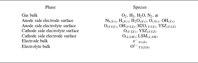
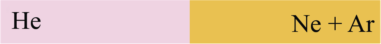
Figure 2. Sketch of the initial conditions in the capillary tube.
The ends of the computational domain were supplied from inlets with a mixture having the same composition as that with which they were initialised. The temperature of the incoming mixture is $300\, \textrm {K}$
and the pressure was equal to the initial pressure corresponding to the test case. The inlet boundary condition for the lattice Boltzmann populations was imposed by replacing only the missing populations, following the method which has been described in detail as a ‘simplified flux boundary condition’ by Sawant et al. (Reference Sawant, Dorschner and Karlin2022). To evaluate the binary diffusion coefficients
$300\, \textrm {K}$
and the pressure was equal to the initial pressure corresponding to the test case. The inlet boundary condition for the lattice Boltzmann populations was imposed by replacing only the missing populations, following the method which has been described in detail as a ‘simplified flux boundary condition’ by Sawant et al. (Reference Sawant, Dorschner and Karlin2022). To evaluate the binary diffusion coefficients $\mathcal{D}_{ab}$
from the Cantera (Goodwin et al. Reference Goodwin, Moffat, Schoegl, Speth and Weber2018) package, we used the parameters pertaining to Lennard-Jones potential for helium, neon and argon based on Tee et al. (Reference Tee, Gotoh and Stewart1966), Klopper (Reference Klopper2001), Tchouar et al. (Reference Tchouar, Benyettou and Kadour2003) and Nasrabad et al. (Reference Nasrabad, Laghaei and Deiters2004), respectively. For a capillary tube with a diameter
$\mathcal{D}_{ab}$
from the Cantera (Goodwin et al. Reference Goodwin, Moffat, Schoegl, Speth and Weber2018) package, we used the parameters pertaining to Lennard-Jones potential for helium, neon and argon based on Tee et al. (Reference Tee, Gotoh and Stewart1966), Klopper (Reference Klopper2001), Tchouar et al. (Reference Tchouar, Benyettou and Kadour2003) and Nasrabad et al. (Reference Nasrabad, Laghaei and Deiters2004), respectively. For a capillary tube with a diameter $d_0=39\, \rm \mu m$
, the Knudsen diffusion coefficients
$d_0=39\, \rm \mu m$
, the Knudsen diffusion coefficients $\mathcal{D}_{a}^{ {k}}$
(Mason et al. Reference Mason, Malinauskas and Malinauskas1983) were calculated as
$\mathcal{D}_{a}^{ {k}}$
(Mason et al. Reference Mason, Malinauskas and Malinauskas1983) were calculated as
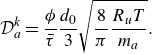 \begin{align} {\mathcal{D}_{a}^{ {k}} = \frac {\phi }{\bar \tau } \frac {d_0}{3} \sqrt {\frac {8}{\pi } \frac {R_u T}{m_a}}}. \end{align}
For this specific test case, since the capillary tube is fully open, the porosity $\phi =1$
and the tortuosity
$\phi =1$
and the tortuosity $\bar \tau =1$
because the capillary tube is straight. Since the tube diameter, the porosity and the tortuosity are the only parameters from the physical set-up entering the model, it is an excellent candidate to test a formulation for DGM because this test case does not involve any tuneable free parameters. For the purpose of comparison, the component mass diffusion fluxes
$\bar \tau =1$
because the capillary tube is straight. Since the tube diameter, the porosity and the tortuosity are the only parameters from the physical set-up entering the model, it is an excellent candidate to test a formulation for DGM because this test case does not involve any tuneable free parameters. For the purpose of comparison, the component mass diffusion fluxes $\rho _a \boldsymbol{V}_a$
obtained through (2.4) and (2.30) are converted to physical units and divided by their molecular weights
$\rho _a \boldsymbol{V}_a$
obtained through (2.4) and (2.30) are converted to physical units and divided by their molecular weights $m_a$
to get the molar diffusion fluxes
$m_a$
to get the molar diffusion fluxes $N_a$
. At the steady state, the molar diffusion flux of helium, and the negative of the molar diffusion fluxes of neon and argon which flows in the opposite direction are plotted in figure 3. The fluxes from the lattice Boltzmann simulations compare well with the fluxes reported from experiments by Remick & Geankoplis (Reference Remick and Geankoplis1974). The model has reproduced the correct flux in the molecular diffusion regime at the higher pressures, the transition regime at moderate pressures as well as at the Knudsen diffusion dominated regime at low pressures. This test instils confidence that the DGM has been correctly formulated and realised in the lattice Boltzmann framework.
$N_a$
. At the steady state, the molar diffusion flux of helium, and the negative of the molar diffusion fluxes of neon and argon which flows in the opposite direction are plotted in figure 3. The fluxes from the lattice Boltzmann simulations compare well with the fluxes reported from experiments by Remick & Geankoplis (Reference Remick and Geankoplis1974). The model has reproduced the correct flux in the molecular diffusion regime at the higher pressures, the transition regime at moderate pressures as well as at the Knudsen diffusion dominated regime at low pressures. This test instils confidence that the DGM has been correctly formulated and realised in the lattice Boltzmann framework.
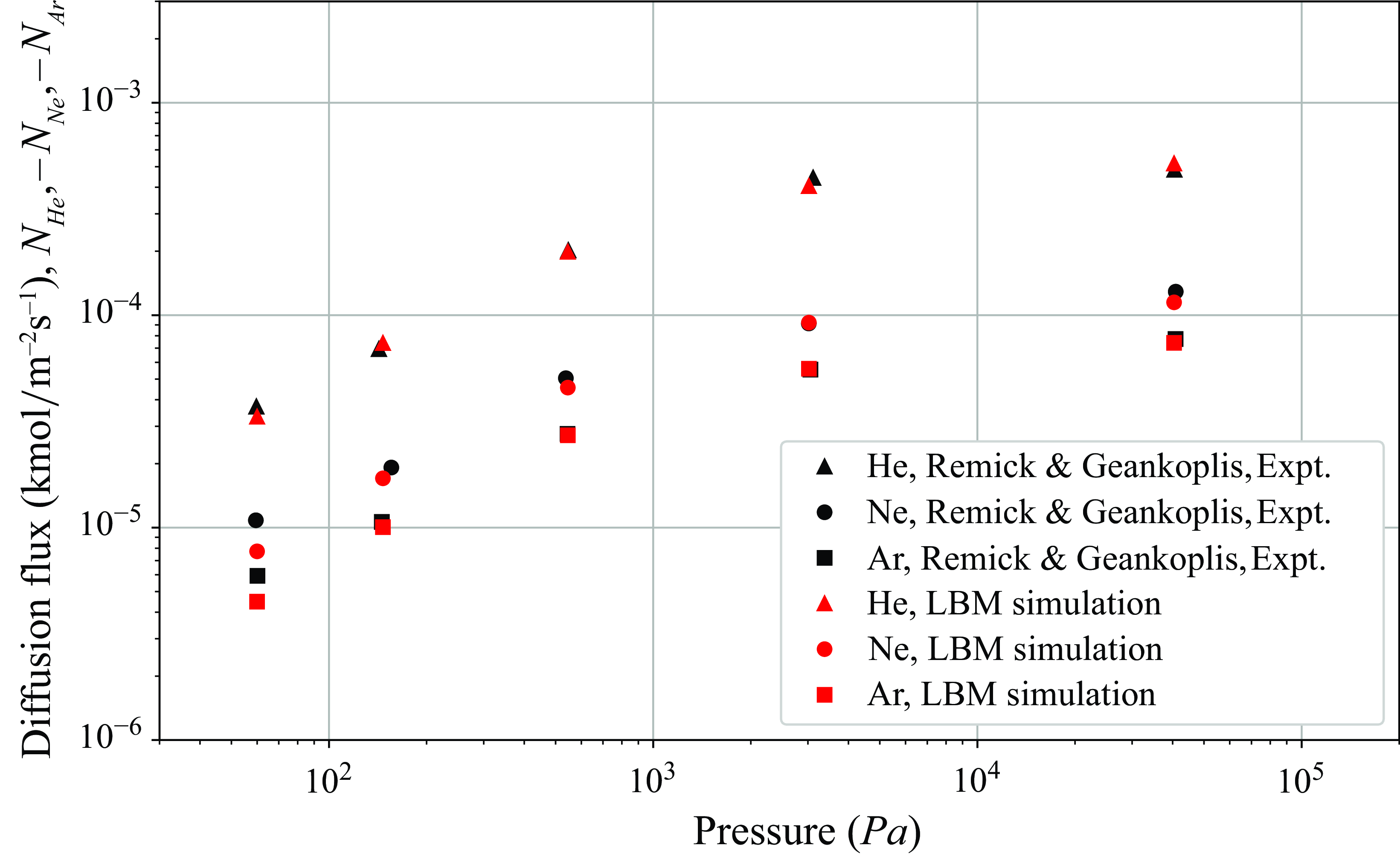
Figure 3. Molar flux of helium counter diffusing against neon and argon in a $39\, \rm \mu m$
wide and
$39\, \rm \mu m$
wide and $9.6\,\rm mm$
long capillary tube. One-dimensional LBM simulations compared with experiments from Remick & Geankoplis (Reference Remick and Geankoplis1974) performed at different pressures ranging from
$9.6\,\rm mm$
long capillary tube. One-dimensional LBM simulations compared with experiments from Remick & Geankoplis (Reference Remick and Geankoplis1974) performed at different pressures ranging from $60$
to
$60$
to $40\,422\, \rm Pa$
.
$40\,422\, \rm Pa$
.
5.2. Solid oxide fuel cell simulation
The LBM is used to perform 1-D $\textrm {1D}$
simulations of an SOFC member electrode assembly at different porosities and current densities with an intent to obtain polarisation curves, verifiable against the literature. As described in § 2.2, we use the standard
$\textrm {1D}$
simulations of an SOFC member electrode assembly at different porosities and current densities with an intent to obtain polarisation curves, verifiable against the literature. As described in § 2.2, we use the standard $D3Q27$
lattice albeit with periodic boundary conditions in two directions to achieve a 1-D computational domain. We recall that, since we are working within the REV formulation, a 1-D computational domain is sufficient to represent the 3-D microstructure of the porous electrodes through parameters such as the porosity, specific areas and specific lengths. A sketch of the simulation domain is shown in figure 1 to aid visualisation of the geometry. The length of the impervious electrolyte section in the middle of the set-up is
$D3Q27$
lattice albeit with periodic boundary conditions in two directions to achieve a 1-D computational domain. We recall that, since we are working within the REV formulation, a 1-D computational domain is sufficient to represent the 3-D microstructure of the porous electrodes through parameters such as the porosity, specific areas and specific lengths. A sketch of the simulation domain is shown in figure 1 to aid visualisation of the geometry. The length of the impervious electrolyte section in the middle of the set-up is $8 \;\rm \mu m$
, while the total length of the cell is
$8 \;\rm \mu m$
, while the total length of the cell is $150 \;\rm \mu m$
.
$150 \;\rm \mu m$
.
We use the electrochemical and heterogeneous reaction mechanisms from DeCaluwe et al. (Reference DeCaluwe, Zhu, Kee and Jackson2008), consisting of five gas phase species, O2, H2, H2O, N2 and Ar. In addition to the gas phase species, the mechanism also contains species which exist as adsorbed species on the surfaces of the anode material $_{( {Ni})}$
, cathode material
$_{( {Ni})}$
, cathode material $_{( {LSM})}$
and the electrolyte material
$_{( {LSM})}$
and the electrolyte material $_{( {YSZ})}$
. All the species are listed in table 1. The reaction mechanism is a compilation of anode reactions from Bessler et al. (Reference Bessler, Warnatz and Goodwin2007a
), cathode reactions from Jiang (Reference Jiang1998), charge transfer reactions from Singhal et al. (Reference Singhal2005) and thermodynamic parameters from various other sources (Gordon Reference Gordon1994; McBride Reference McBride1996; Janardhanan & Deutschmann Reference Janardhanan and Deutschmann2006; Bessler et al. Reference Bessler, Gewies and Vogler2007b
).
$_{( {YSZ})}$
. All the species are listed in table 1. The reaction mechanism is a compilation of anode reactions from Bessler et al. (Reference Bessler, Warnatz and Goodwin2007a
), cathode reactions from Jiang (Reference Jiang1998), charge transfer reactions from Singhal et al. (Reference Singhal2005) and thermodynamic parameters from various other sources (Gordon Reference Gordon1994; McBride Reference McBride1996; Janardhanan & Deutschmann Reference Janardhanan and Deutschmann2006; Bessler et al. Reference Bessler, Gewies and Vogler2007b
).
Apart from the gas phase and the adsorbed surface phase species, the electrons $\mathrm{e^-}_{{Ni}({b})}$
reside in the bulk electrode phase while the oxide ions
$\mathrm{e^-}_{{Ni}({b})}$
reside in the bulk electrode phase while the oxide ions $\mathrm{O^{2-}}_{{YSZ}( {b})}$
reside in the bulk of the electrolyte phase. In this paper, we do not model the transport inside these solid bulk phases. In the unit of mole fractions, the anode is uniformly initialised with a composition of {H2 0.97, H2O 0.03}, whereas the cathode is uniformly initialised with a composition of {O2 0.21, N2 0.78, Ar 0.01}.
$\mathrm{O^{2-}}_{{YSZ}( {b})}$
reside in the bulk of the electrolyte phase. In this paper, we do not model the transport inside these solid bulk phases. In the unit of mole fractions, the anode is uniformly initialised with a composition of {H2 0.97, H2O 0.03}, whereas the cathode is uniformly initialised with a composition of {O2 0.21, N2 0.78, Ar 0.01}.
Throughout the simulation, the electrodes are supplied from the inlets with a mixture having the same composition as the compositionwith which they were initialised. An inlet boundary condition is used at both ends of the computational domain to supply the respective mixtures at a pressure of one atmosphere and a temperature of $1073.15\, \textrm {K}$
. The inlet boundary condition, which has been imposed by only replacing the missing populations, has been described in detail as a ‘simplified flux boundary condition’ by Sawant et al. (Reference Sawant, Dorschner and Karlin2022). The inlet flux boundary condition prescribes the composition of the incoming mixture, without strictly imposing the composition of outgoing flux, making it ideal for this 1-D computational domain in which the products leave the domain through the inlet. At the interface of the porous electrode section with the impervious electrolyte section, the bounce back boundary condition is applied on the missing populations of the species lattice as well the on the missing populations of the mean field momentum lattice and the energy lattice. At the macroscopic level, the application of the bounce back boundary condition results in no flux, no slip and adiabatic conditions at the interface (He et al. Reference He, Chen and Doolen1998). For this test case, this means that the gasesous species do not enter the solid electrolyte region in the middle of the membrane electrode assembly. The reactants travel through the reactive porous electrodes upto the electrode–electrolyte interface and stagnate at the interface, while the products travel outwards from where they are produced in the region near the electrode–electrolyte interface outward towards the open ends of the computational domain.
$1073.15\, \textrm {K}$
. The inlet boundary condition, which has been imposed by only replacing the missing populations, has been described in detail as a ‘simplified flux boundary condition’ by Sawant et al. (Reference Sawant, Dorschner and Karlin2022). The inlet flux boundary condition prescribes the composition of the incoming mixture, without strictly imposing the composition of outgoing flux, making it ideal for this 1-D computational domain in which the products leave the domain through the inlet. At the interface of the porous electrode section with the impervious electrolyte section, the bounce back boundary condition is applied on the missing populations of the species lattice as well the on the missing populations of the mean field momentum lattice and the energy lattice. At the macroscopic level, the application of the bounce back boundary condition results in no flux, no slip and adiabatic conditions at the interface (He et al. Reference He, Chen and Doolen1998). For this test case, this means that the gasesous species do not enter the solid electrolyte region in the middle of the membrane electrode assembly. The reactants travel through the reactive porous electrodes upto the electrode–electrolyte interface and stagnate at the interface, while the products travel outwards from where they are produced in the region near the electrode–electrolyte interface outward towards the open ends of the computational domain.
For the purpose of validation, we aim to replicate polarisation curves from the experiments performed on solid oxide button cells by Zhao & Virkar (Reference Zhao and Virkar2005). DeCaluwe et al. (Reference DeCaluwe, Zhu, Kee and Jackson2008)reproduced the curves through a finite volume DGM discretisation in conjunction with a set of detailed reaction mechanisms, the latter of which is also used in this work in conjunction with the proposed LBM. To that end, simulations are performed for three values of anode porosity, $0.57$
,
$0.57$
, $0.48$
and
$0.48$
and $0.32$
, while the cathode porosity is kept constant at
$0.32$
, while the cathode porosity is kept constant at $0.45$
. In the experiments of Zhao & Virkar (Reference Zhao and Virkar2005), the porosity of the electrodes was determined by quantitative stereology using the systematic point count procedure (Underwood Reference Underwood, McCall and Mueller1973). In reality, the length of the electrochemically active layer in the porous electrodes is determined by the transport of the
$0.45$
. In the experiments of Zhao & Virkar (Reference Zhao and Virkar2005), the porosity of the electrodes was determined by quantitative stereology using the systematic point count procedure (Underwood Reference Underwood, McCall and Mueller1973). In reality, the length of the electrochemically active layer in the porous electrodes is determined by the transport of the $\mathrm{O^{2-}}_{{YSZ}( {b})}$
ions through the bulk of the electrolyte. Since we do not model the ion transport through the bulk electrolyte, it is not possible to know the length of the electrochemically active layer in the porous electrodes. Consistent with other studies performed under the same limitations, including that of DeCaluwe et al. (Reference DeCaluwe, Zhu, Kee and Jackson2008), the length of the active layer, also called the ‘utilisation thickness’
$\mathrm{O^{2-}}_{{YSZ}( {b})}$
ions through the bulk of the electrolyte. Since we do not model the ion transport through the bulk electrolyte, it is not possible to know the length of the electrochemically active layer in the porous electrodes. Consistent with other studies performed under the same limitations, including that of DeCaluwe et al. (Reference DeCaluwe, Zhu, Kee and Jackson2008), the length of the active layer, also called the ‘utilisation thickness’ $\delta _{ {util}}$
, as well as the length of the triple phase boundary
$\delta _{ {util}}$
, as well as the length of the triple phase boundary $l_{ {T\!P\!B}}^{(e)}$
are treated as free parameters. Their values used in the LBM simulations are reported in table 2. The utilisation thickness has an inverse relation to porosity as expected (Divisek et al. Reference Divisek, Jung and Vinke1999; Chan & Xia Reference Chan and Xia2001). The size of the utilisation thickness in the simulation is controlled by changing the resolution. A lattice resolution of
$l_{ {T\!P\!B}}^{(e)}$
are treated as free parameters. Their values used in the LBM simulations are reported in table 2. The utilisation thickness has an inverse relation to porosity as expected (Divisek et al. Reference Divisek, Jung and Vinke1999; Chan & Xia Reference Chan and Xia2001). The size of the utilisation thickness in the simulation is controlled by changing the resolution. A lattice resolution of $\delta x = 1\rm \mu m$
is used for
$\delta x = 1\rm \mu m$
is used for $\phi =0.57$
simulation and the resolution is changed to vary the utilisation length. The product of utilisation thickness and specific surface area
$\phi =0.57$
simulation and the resolution is changed to vary the utilisation length. The product of utilisation thickness and specific surface area $\delta _{ {util}} a^{(s)}$
is
$\delta _{ {util}} a^{(s)}$
is $20$
for all surfaces and all simulations. The values for specific surface areas have been adopted from DeCaluwe et al. (Reference DeCaluwe, Zhu, Kee and Jackson2008), who had estimated those values by assuming an average particle size of
$20$
for all surfaces and all simulations. The values for specific surface areas have been adopted from DeCaluwe et al. (Reference DeCaluwe, Zhu, Kee and Jackson2008), who had estimated those values by assuming an average particle size of $d^{(p)}=2.5 \,\rm \mu m$
and an average pore radius of
$d^{(p)}=2.5 \,\rm \mu m$
and an average pore radius of $d_0 = 0.5\, \rm \mu m$
. A REV made up of synthetic spherical microstructures of these specifications is shown in figure 9. If necessitated by the transport model (Zhu & Kee Reference Zhu and Kee2003; Zhu et al. Reference Zhu, Kee, Janardhanan, Deutschmann and Goodwin2005), the particle size can be used to estimate permeability using the Kozeny–Carman equation (Kozeny Reference Kozeny1927; Carman Reference Carman1997) as follows.
$d_0 = 0.5\, \rm \mu m$
. A REV made up of synthetic spherical microstructures of these specifications is shown in figure 9. If necessitated by the transport model (Zhu & Kee Reference Zhu and Kee2003; Zhu et al. Reference Zhu, Kee, Janardhanan, Deutschmann and Goodwin2005), the particle size can be used to estimate permeability using the Kozeny–Carman equation (Kozeny Reference Kozeny1927; Carman Reference Carman1997) as follows.
Table 2. Parameters corresponding to simulations performed at different porosity.
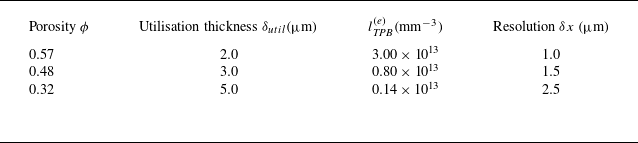
Assuming a porous packed bed of identical spherical particles, each of diameter $d^{(p)}$
, the specific surface area
$d^{(p)}$
, the specific surface area $a^{(p)}$
of the microstructure can be approximated as
$a^{(p)}$
of the microstructure can be approximated as
 \begin{align} a^{(p)} = \frac {6}{d^{(p)}}. \end{align}
With the specific surface area being known, it can be used to compute the hydraulic radius $r^{(p)}$
with the expression
$r^{(p)}$
with the expression
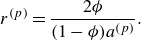 \begin{align} r^{(p)} = \frac {2 \phi }{(1 - \phi ) a^{(p)}}. \end{align}
Assuming unit tortuosity, the permeability $\mathcal B$
can be approximated from hydraulic radius and porosity,
$\mathcal B$
can be approximated from hydraulic radius and porosity,
 \begin{align} \mathcal B = \frac {\phi }{8} r^{(p)^2} . \end{align}
The permeability can be used to approximate a retardation using Darcy’s law. On the lines of extended velocity $u_{\alpha }^{ {ex}}$
which is defined in this model by (3.15), an alternate way of penalising the momentum equation is through Darcy’s law by incorporating the resultant retardation through the extended Darcy velocity
$u_{\alpha }^{ {ex}}$
which is defined in this model by (3.15), an alternate way of penalising the momentum equation is through Darcy’s law by incorporating the resultant retardation through the extended Darcy velocity $u_{\alpha }^{ {ex} D}$
,
$u_{\alpha }^{ {ex} D}$
,
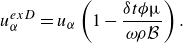 \begin{align} u_{\alpha }^{ {ex} D} = u_{\alpha }\left (1 - \frac { \delta t \phi \mu }{\omega \rho \mathcal B} \right ) . \end{align}
Although we have presented the above discussion on Darcy force for completeness, we emphasise that in our model, we use the pore size to compute the Knudsen diffusivity from (5.1), which enters the extended velocity $u_{\alpha }^{ {ex}}$
defined by (3.15), via a penalising force defined by (3.16).
$u_{\alpha }^{ {ex}}$
defined by (3.15), via a penalising force defined by (3.16).
The SOFC operates at atmospheric pressure and therefore, the Knudsen effect due to rarefaction is not expected to dominate over the dynamics of the system. However, it should be emphasised that the DGM formulated in this work enables the simulation to account for the effect of porosity as a parameter though the Knudsen diffusion term appended to the Stefan–Maxwell model and the resulting penalisation term in the momentum equation.
Although we do not model the transport of individual ions, we solve the charge transport equations (4.9) and (4.10) in the solid electrolyte, including the impervious section and using the values of resistivity from Zhao & Virkar (Reference Zhao and Virkar2005). Therefore, the middle impervious electrolyte section does cause a drop in the cell potential due to resistance of the electrolyte phase. The electrolyte phase in the anode section is set to $0$
V and the metal electrode phase is set at a certain potential above the open circuit voltage so that a certain current density is produced in the anode. This current density is then imposed at the cathode and a reverse problem is solved, i.e. an electrode potential which produces the same current is found iteratively by the Newton–Raphson method.
$0$
V and the metal electrode phase is set at a certain potential above the open circuit voltage so that a certain current density is produced in the anode. This current density is then imposed at the cathode and a reverse problem is solved, i.e. an electrode potential which produces the same current is found iteratively by the Newton–Raphson method.
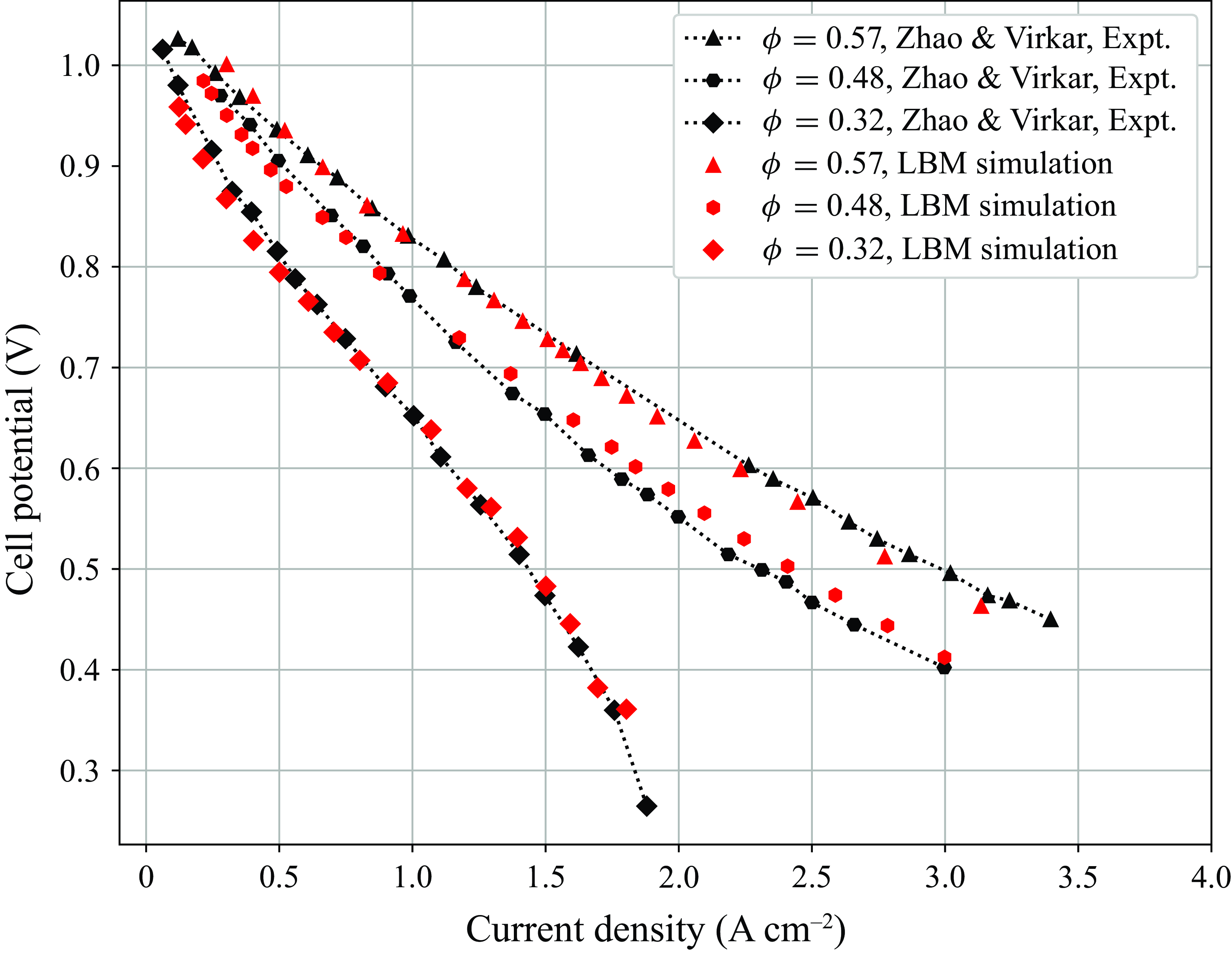
Figure 4. Cell potential versus current density.
The polarisation curves obtained from the simulation have been compared against the experimental data of Zhao & Virkar (Reference Zhao and Virkar2005). Figure 4 compares the voltage versus current density whereas figure 5 compares power versus the current density. From both the figures, it is evident that a reasonable match has been obtained with respect to the experimental data for all three values of porosity in the regime of low as well as medium and high current densities. The model captures losses in all three regimes: the activation overpotential occuring at low current density originating from activation of the electrochemical reactions, the ohmic overpotential occuring at moderate current density originating from the loss due to internal resistance and the concentration overpotential occuring at high current density due to limitation on the transport of the reactants in the porous electrodes. The effect of concentration overpotential is unmistakably visible in the polarisation curve for $\phi =0.32$
after the current density
$\phi =0.32$
after the current density $1.5 \; \rm A\, cm^{-2}$
. Good agreement with the experiments is an indication that modelling of the chemistry, charge continuity, and most importantly the species transport with associated momentum and energy modelling has been achieved correctly. In our future work, we intend to implement not only tortuosity as a parameter, but also model the ion transport in the bulk electrolyte which will make it possible to obtain the utilisation length as an output from the simulation rather than as an input parameter. Since simulations with detailed chemistry as well as hydrodynamics have been performed, there is an opportunity to peek into the porous electrodes to observe the state of various variables that have been modelled. In figure 6, a data point has been selected for plotting the composition, temperature and potential along the length of the composite electrodes. The data point corresponds to a
$1.5 \; \rm A\, cm^{-2}$
. Good agreement with the experiments is an indication that modelling of the chemistry, charge continuity, and most importantly the species transport with associated momentum and energy modelling has been achieved correctly. In our future work, we intend to implement not only tortuosity as a parameter, but also model the ion transport in the bulk electrolyte which will make it possible to obtain the utilisation length as an output from the simulation rather than as an input parameter. Since simulations with detailed chemistry as well as hydrodynamics have been performed, there is an opportunity to peek into the porous electrodes to observe the state of various variables that have been modelled. In figure 6, a data point has been selected for plotting the composition, temperature and potential along the length of the composite electrodes. The data point corresponds to a $\phi =0.57$
cell while it produces a current density of approximately
$\phi =0.57$
cell while it produces a current density of approximately $1\, \rm A\, cm^{-2}$
. In the figure, the gas phase composition is seen to have an appreciable change only near the interfaces with the impervious electrolyte. On the left side of the figure, which is the anode section, gaseous
$1\, \rm A\, cm^{-2}$
. In the figure, the gas phase composition is seen to have an appreciable change only near the interfaces with the impervious electrolyte. On the left side of the figure, which is the anode section, gaseous $\textrm {H}_2$
is seen to have a drop in mass fraction accompanied by a rise in the gaseous
$\textrm {H}_2$
is seen to have a drop in mass fraction accompanied by a rise in the gaseous $\mathrm{H}_2\mathrm{O}$
in the topmost frame. This is an indication of the oxidation of hydrogen by the oxide ions, resulting in water. On the cathode section on the right-hand side, there is a drop in to mass fraction of
$\mathrm{H}_2\mathrm{O}$
in the topmost frame. This is an indication of the oxidation of hydrogen by the oxide ions, resulting in water. On the cathode section on the right-hand side, there is a drop in to mass fraction of $\mathrm{O}_2$
, as it gets converted into oxide ions. The figure also shows mole fractions of adsorbed species and temperature, which do not show appreciable change in the linear scale. In the bottom most frame of the figure, the drop in potential due to the resistance of the electrolyte phase is visible across the impervious electrolyte section, labelled as ‘oxide pot.’. The metal phase potential is negative on the anode side of the cell and positive on the cathode side of the cell as expected. In the accompanying figure 7, panel (a) shows a peak in the volumetric current density due to the generation of electrons at the anode–electrolyte section interface and a second peak due the consumption of electrons at the cathode–electrolyte section interface. We plot the current as positive even though the rate of production of electrons is negative in the cathode. The profile in figure 7(b) is that of the area current density, which is an integrated quantity. In the simulation, the current density generated at the anode is imposed as a boundary condition on the cathode and a corresponding cathode voltage is computed. The decrease of the current density in the cathode section shows that the cell is correctly charge balanced and ‘connected’, i.e. all the electrons created by the electrochemical reactions at the anode are consumed by the electrochemical reactions at the cathode.
$\mathrm{O}_2$
, as it gets converted into oxide ions. The figure also shows mole fractions of adsorbed species and temperature, which do not show appreciable change in the linear scale. In the bottom most frame of the figure, the drop in potential due to the resistance of the electrolyte phase is visible across the impervious electrolyte section, labelled as ‘oxide pot.’. The metal phase potential is negative on the anode side of the cell and positive on the cathode side of the cell as expected. In the accompanying figure 7, panel (a) shows a peak in the volumetric current density due to the generation of electrons at the anode–electrolyte section interface and a second peak due the consumption of electrons at the cathode–electrolyte section interface. We plot the current as positive even though the rate of production of electrons is negative in the cathode. The profile in figure 7(b) is that of the area current density, which is an integrated quantity. In the simulation, the current density generated at the anode is imposed as a boundary condition on the cathode and a corresponding cathode voltage is computed. The decrease of the current density in the cathode section shows that the cell is correctly charge balanced and ‘connected’, i.e. all the electrons created by the electrochemical reactions at the anode are consumed by the electrochemical reactions at the cathode.

Figure 5. Power density versus current density.
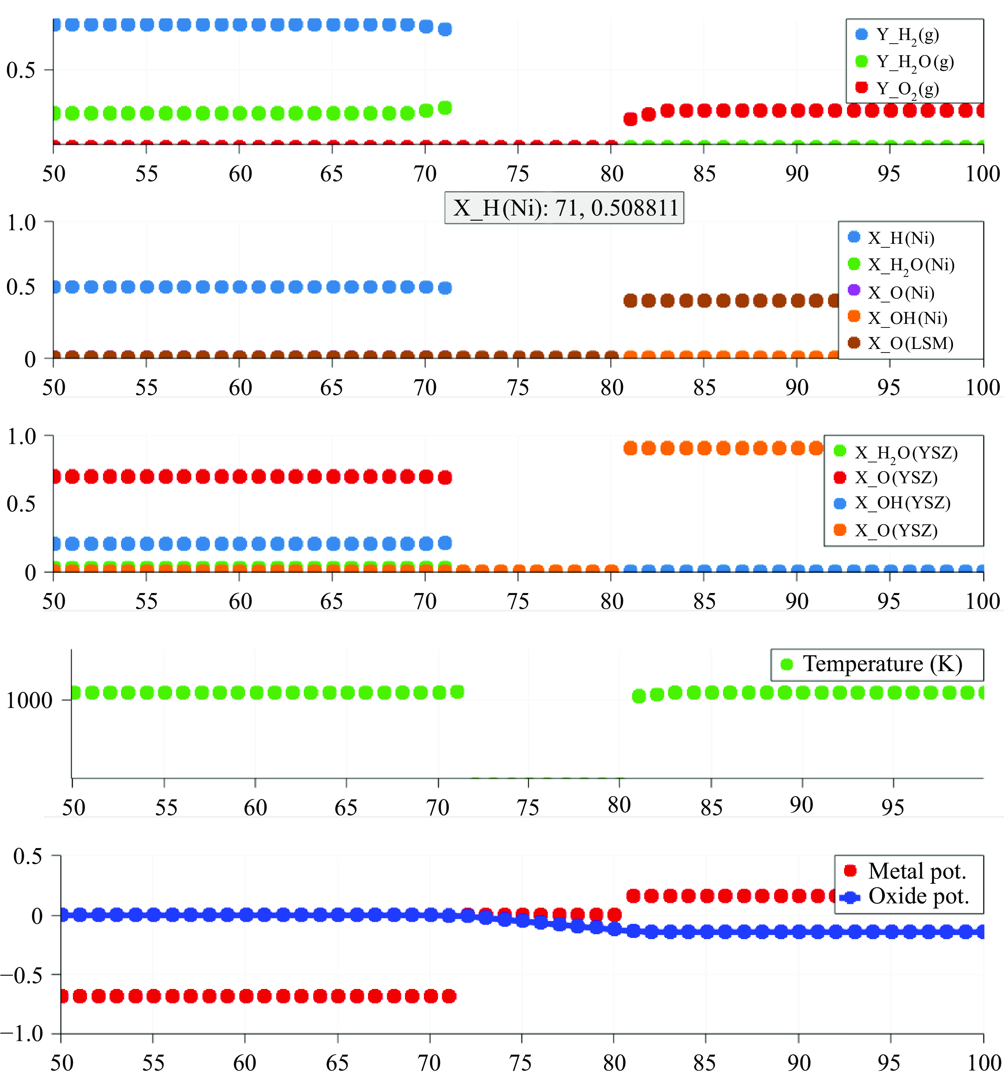
Figure 6. Top to bottom: mass fraction of the gas phase species, mole fraction of the species adsorbed on the electrode surface, mole fractions of the species adsorbed on the electrolyte surface, temperature and potential along the length of the MEA. Porosity is $\phi =0.57$
and the current density is
$\phi =0.57$
and the current density is $1.05 \; \rm A\, cm^{-2}$
.
$1.05 \; \rm A\, cm^{-2}$
.

Figure 7. Top to bottom: current density per unit volume $\mathcal{I}^{ {(v)}}(x)$
and current density per unit area
$\mathcal{I}^{ {(v)}}(x)$
and current density per unit area $\mathcal{I}^{ {(a)}}(x)$
along the length of the MEA. Porosity is
$\mathcal{I}^{ {(a)}}(x)$
along the length of the MEA. Porosity is $\phi =0.57$
and the current density is
$\phi =0.57$
and the current density is $1.05 \; \rm A\, cm^{-2}$
.
$1.05 \; \rm A\, cm^{-2}$
.
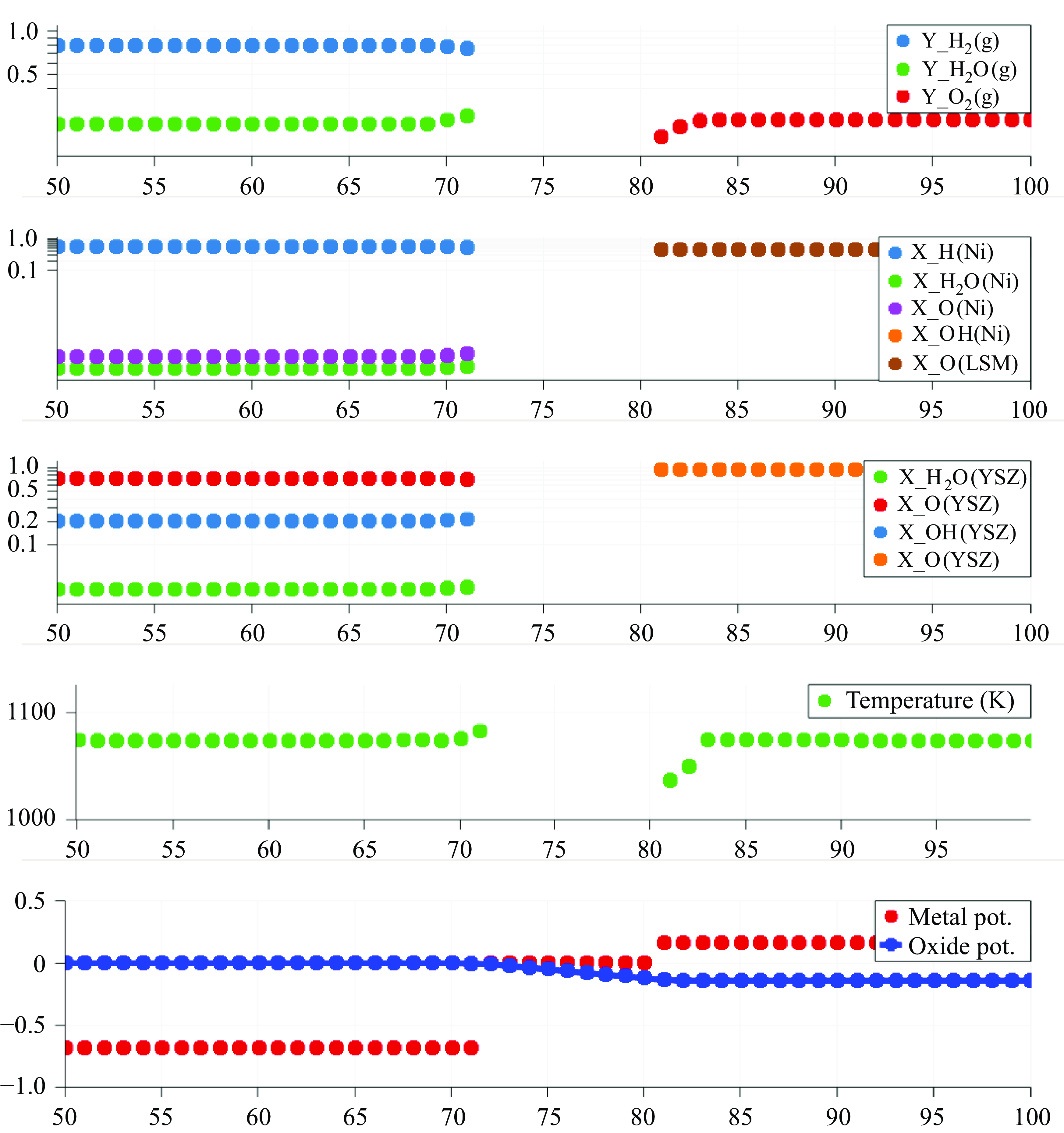
Figure 8. Top to bottom in log scale: mass fraction of the gas phase species, mole fraction of the species adsorbed on the electrode surface and mole fractions of the species adsorbed on the electrolyte surface. In linear scale: temperature and potential along the length of the MEA. Porosity is $\phi =0.57$
and the current density is
$\phi =0.57$
and the current density is $1.05 \; \rm A\, cm^{-2}$
.
$1.05 \; \rm A\, cm^{-2}$
.
Figure 8 presents the same information as in figure 6, with a change in the $y$
-axis scaling. The mass and the mole fractions are plotted in the log scale to make the species with low mole fractions more visible. For example, in the second panel from the top, the adsorbed oxygen and adsorbed water on the nickel surface in the anode section can be seen to have a small increase in the mole fraction at the interface with the electrolyte section. There is a similar increase at the interface in the oxygen and the hydroxide adsorbed on the YSZ surface at the anode, visible in the third panel from the top. Perhaps the most interesting part of figure 8 is the temperature profile. The oxidation reaction atthe anode being exothermic is seen to have caused an increase in the temperature whereas the endothermic oxidation (Xia et al. Reference Xia, Oldman and Catlow2012) at the cathode is seen to have produced a drop in the temperature in the electrochemically active region. These temperature dynamics reveal an interesting opportunity to also compute the heat conduction in the electrolyte phase, which will be undertaken as part of our future work.
$y$
-axis scaling. The mass and the mole fractions are plotted in the log scale to make the species with low mole fractions more visible. For example, in the second panel from the top, the adsorbed oxygen and adsorbed water on the nickel surface in the anode section can be seen to have a small increase in the mole fraction at the interface with the electrolyte section. There is a similar increase at the interface in the oxygen and the hydroxide adsorbed on the YSZ surface at the anode, visible in the third panel from the top. Perhaps the most interesting part of figure 8 is the temperature profile. The oxidation reaction atthe anode being exothermic is seen to have caused an increase in the temperature whereas the endothermic oxidation (Xia et al. Reference Xia, Oldman and Catlow2012) at the cathode is seen to have produced a drop in the temperature in the electrochemically active region. These temperature dynamics reveal an interesting opportunity to also compute the heat conduction in the electrolyte phase, which will be undertaken as part of our future work.
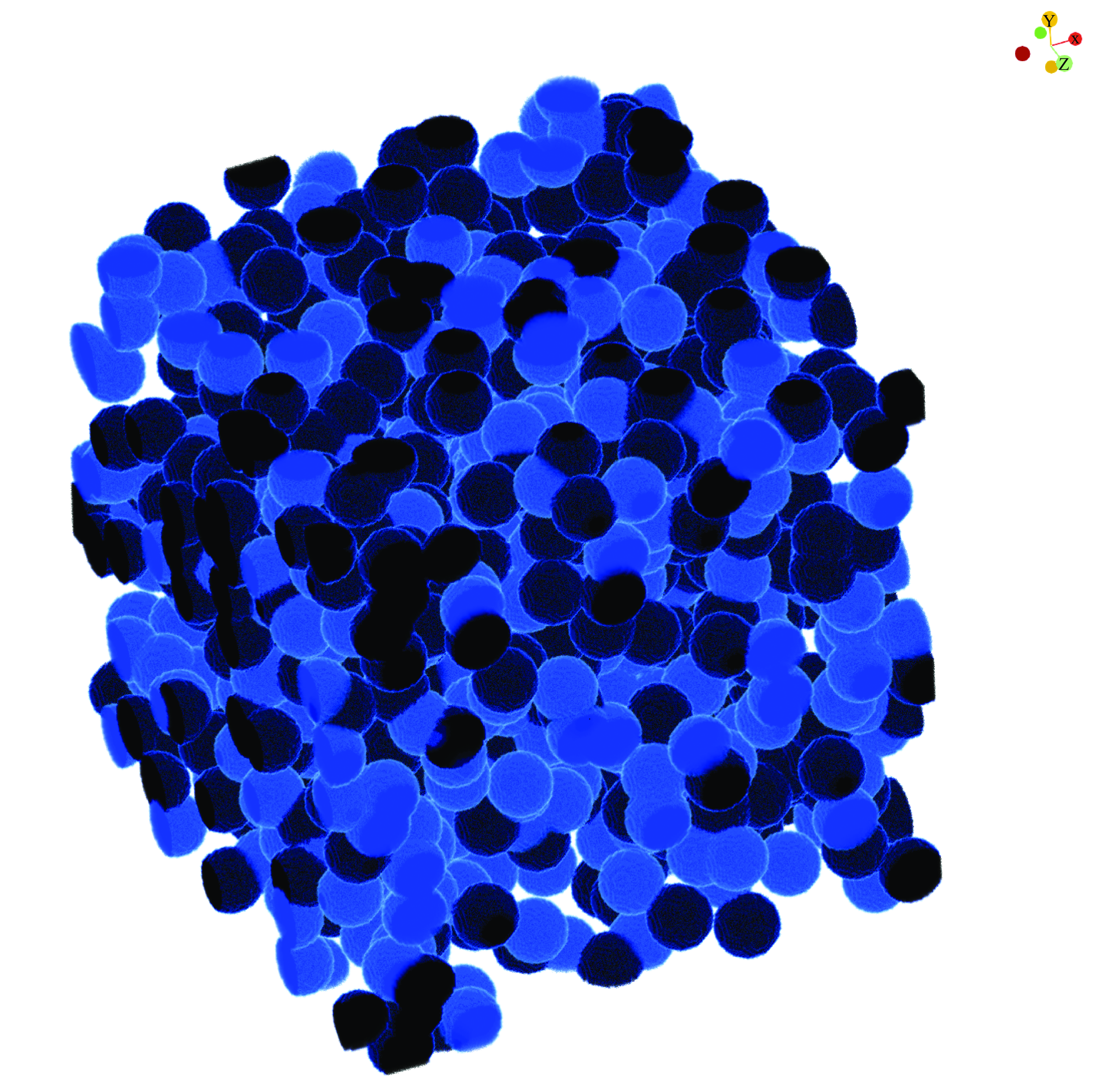
Figure 9. A synthetic microstructure with $2.5\, \rm \mu m$
blue and black spheres representing the electrolyte and the electrode phase, respectively. The empty space between the spheres represents the hollow space with porosity
$2.5\, \rm \mu m$
blue and black spheres representing the electrolyte and the electrode phase, respectively. The empty space between the spheres represents the hollow space with porosity $\phi =0.57$
for the gas phase. The cube has sides of
$\phi =0.57$
for the gas phase. The cube has sides of $25 \,\rm \mu m$
each, representing a hypothetical REV of an SOFC anode.
$25 \,\rm \mu m$
each, representing a hypothetical REV of an SOFC anode.
6. Conclusion
In this work, we started with a reactive multi-component compressible lattice Boltzmann model with Stefan–Maxwell diffusion. In § 2, we converted the Stefan–Maxwell diffusion model to the DGM. Next, the LBM was re-designed to obtain a representative elementary volume hydrodynamic model for porous media in § 3. The resulting dusty gas– lattice Boltzmann model was validated by computing counter-diffusion molar fluxes through capillary tubes in § 5.1. Furthermore, the model was extended to include heterogeneous surface and electrochemical reactions in § 4. The complete LBM for porous electrochemical flows was used to perform simulations of flow in solid oxide fuel cell electrodes and polarisation curves were compared against experiments in § 5.2.
To recap, through this work, we have developed a lattice Boltzmann model which encompasses detailed electrochemistry, multi-component mass transport and fluid dynamics for realistic simulations of fuel cells. Such a model is not only a starting point to reveal the rich interplay between chemical reactions, fluid flow, species composition and current density at the pore scale, but also has a potential to function as a digital twin for developing and optimising practical fuel cell microstructures and geometries at a reasonable compute cost. In a reduced form, the model can also be used to study single-component or non-reactive flows in porous media, which is of much relevance to the geophysics community (Philip Reference Philip1970; Winter & Tartakovsky Reference Winter and Tartakovsky2000). Since the model at its core is an extension of a compressible lattice Boltzmann model to porous media, the model also has other potential applications including, but not limited to, petroleum engineering (Jönsson & Jönsson, Reference Jönsson and Jönsson1992; Zidane & Firoozabadi Reference Zidane and Firoozabadi2014).
In a further development, we intend to reduce the free parameters in the model by accommodating more physics. To that end, a model for ion transport through the solid electrolyte will set the solver free from the necessity to use the utilisation thickness as a parameter. Heat conduction through the solid matrix has to be modelled, which can provide additional opportunities to study the thermal gradients and hence the stresses in the membrane electrode assembly. In addition to the conjugate heat transfer, we also need to account for the capacitance when dealing with the model for electric current if we need to make the model useful for transient simulations. Creation of such a predictive tool is expected to yield theoretical, scientific and practical gains. Mesoscale simulations on full 3-D geometries would provide additional insights into flow, composition and temperature fields in typical fuel cells, and therefore improve our knowledge of physical and chemical processes occurring in fuel cells. A computing framework capable of performing realistic scale simulations of fuel cells will open up interesting opportunities for optimisations pertaining to geometry, operating conditions, fuel composition and internal reforming.
Acknowledgements.
N.S. thanks Steven DeCaluwe at the Colorado School of Mines for the inputs provided by him on the Cantera Users Group.
Funding.
This work was supported by the Swiss National Science Foundation Proposal ‘10.001.232 Mesoscale multiphysics modeling for fuel cells’ and European Research Council (ERC) Advanced Grant No. 834763-PonD. Computational resources at the Swiss National Super Computing Center CSCS were provided under grant No. s1286.
Declaration of interests.
The authors report no conflict of interest.
Appendix. Hydrodynamic limit of the mean-field LBM
We expand the lattice Boltzmann equations (3.10) and (3.11) in Taylor series to second order, using space component notation and summation convention,
 \begin{align} \left [\delta t (\partial _t + c_{i\mu } \partial _\mu ) + \frac {\delta t^2}{2} (\partial _t + c_{i\mu } \partial _\mu )^2\right ] f_i &= { \omega _{ {B}} (f_i^{ {eq}} -f_i^{ {B}}) + \omega (f_i^{ {B}} -f_i) }, \end{align}
 \begin{align} \left [\delta t (\partial _t + c_{i\mu } \partial _\mu ) + \frac {\delta t^2}{2} (\partial _t + c_{i\mu } \partial _\mu )^2\right ] g_i &= \omega _1 (g_i^{ {eq}} -g_i) + (\omega - \omega _1) (g_i^* -g_i). \end{align}
To obtain the right-hand side of (A1) from (3.10), the substitution $f_i^{ {ex}} = f_i^{ {B}}(1-(\omega _{ {B}}/\omega )) + f_i^{ {eq}} (\omega _{ {B}}/\omega )$
has been used. Such splitting of the extended equilibrium
$f_i^{ {ex}} = f_i^{ {B}}(1-(\omega _{ {B}}/\omega )) + f_i^{ {eq}} (\omega _{ {B}}/\omega )$
has been used. Such splitting of the extended equilibrium $f_i^{ {ex}}$
into a non-equilibrium
$f_i^{ {ex}}$
into a non-equilibrium $f_i^{ {B}}$
and an equilibrium distribution is only done to ease mathematical analysis of the system. The extra relaxation
$f_i^{ {B}}$
and an equilibrium distribution is only done to ease mathematical analysis of the system. The extra relaxation $\omega _{ {B}}$
introduced here vanishes after converting the equation back to the form of
$\omega _{ {B}}$
introduced here vanishes after converting the equation back to the form of $f_i^{ {ex}}$
. With a time scale
$f_i^{ {ex}}$
. With a time scale $\bar t$
and a velocity scale
$\bar t$
and a velocity scale $\bar c$
, the non-dimensional parameters are introduced as follows:
$\bar c$
, the non-dimensional parameters are introduced as follows:
 \begin{equation} t'=\frac {t}{\bar t}, \quad c_{\alpha }'=\frac {c_{\alpha }}{\bar c}, \quad x_{\alpha }'=\frac {x_{\alpha }}{\bar c \bar t}. \end{equation}
Substituting the relations (A3) into (A1) and (A2), the kinetic equations in the non-dimensional form become
 \begin{align} \left [\delta t' (\partial _{t'} + c'_{i\mu } \partial _{\mu '} ) + \frac {\delta t^{\prime 2}}{2} (\partial _{t'} + c'_{i\mu } \partial _{\mu '} )^2\right ] f_i &= { \omega _{ {B}} (f_i^{ {eq}} -f_i^{ {B}}) + \omega (f_i^{ {B}} -f_i) }, \end{align}
 \begin{align} \left [\delta t' (\partial _{t'} + c'_{i\mu } \partial _{\mu '} ) + \frac {\delta t^{\prime 2}}{2} (\partial _{t'} + c'_{i\mu } \partial _{\mu '} )^2\right ] g_i &= \omega _1 (g_i^{ {eq}} -g_i) + (\omega - \omega _1) (g_i^* -g_i). \end{align}
Let us define a smallness parameter $\epsilon$
as
$\epsilon$
as
 \begin{equation} \epsilon =\delta t'=\frac {\delta t}{\bar t}. \end{equation}
Using the definition of $\epsilon$
and dropping the primes for ease of writing, we obtain
$\epsilon$
and dropping the primes for ease of writing, we obtain
 \begin{align} \left [\epsilon (\partial _t + c_{i\mu } \partial _\mu ) + \frac {\epsilon ^2}{2} (\partial _t + c_{i\mu } \partial _\mu )^2\right ] f_i &= { \omega _{ {B}} (f_i^{ {eq}} -f_i^{ {B}}) + \omega (f_i^{ {B}} -f_i) }, \end{align}
 \begin{align} \left [\epsilon (\partial _t + c_{i\mu } \partial _\mu ) + \frac {\epsilon ^2}{2}(\partial _t + c_{i\mu } \partial _\mu )^2\right ] g_i &= \omega _1 (g_i^{ {eq}} -g_i) + (\omega - \omega _1) (g_i^* -g_i). \end{align}
Writing a power series expansion in $\epsilon$
as
$\epsilon$
as
 \begin{align} \partial _t &= \partial _t^{(1)} + \epsilon \partial _t^{(2)}, \end{align}
 \begin{align} f_{i} &= f_{i}^{(0)} + \epsilon f_{i}^{(1)} + \epsilon ^2 f_{i}^{(2)}, \end{align}
 \begin{align} {f_{i}^{ {B}}} & {= f_{i}^{ {B} (0)} + \epsilon f_{i}^{ {B} (1)} + \epsilon ^2 f_{i}^{ {B} (2)},} \end{align}
 \begin{align} g_{i} &= g_{i}^{(0)} + \epsilon g_{i}^{(1)} + \epsilon ^2 g_{i}^{(2)}, \end{align}
 \begin{align} g_{i}^* &= g_{i}^{*(0)} + \epsilon g_{i}^{*(1)} + \epsilon ^2 g_{i}^{*(2)}, \end{align}
we substitute the (A9)–(A13) into (A7) and (A8), and proceed with collecting terms of same order. This procedure is standard (Chapman & Cowling Reference Chapman and Cowling1970); for the specific case of the two-population LBM see, e.g. Karlin et al. (Reference Karlin, Sichau and Chikatamarla2013). At order $\epsilon ^0$
, we get
$\epsilon ^0$
, we get
 \begin{align} f_i^{(0)} & = { f_{i}^{ {B} (0)} } = f_i^{ {eq}}, \end{align}
 \begin{align} g_i^{(0)} &= g_i^{*(0)} = g_i^{ {eq}}. \end{align}
At order $\epsilon ^1$
, upon summation over the discrete velocities, we find
$\epsilon ^1$
, upon summation over the discrete velocities, we find
 \begin{align} &\partial _t^{(1)} \phi \rho + \partial _{\alpha } j_\alpha ^{ {eq}} = 0, \end{align}
 \begin{align} &\partial _t^{(1)} j_\alpha ^{ {eq}} + \partial _\beta P_{\alpha \beta }^{ {eq}} = 0, \end{align}
 \begin{align} &\partial _t^{(1)} ( \phi \rho E) + \partial _{\alpha } q_\alpha ^{ {eq}} = 0. \end{align}
Here, $\rho$
is the density of the fluid given by the zeroth moment of the
$\rho$
is the density of the fluid given by the zeroth moment of the $f$
-populations in (3.5),
$f$
-populations in (3.5), $j_\alpha ^{ {eq}}$
is the equilibrium momentum of the fluid as defined by (3.6),
$j_\alpha ^{ {eq}}$
is the equilibrium momentum of the fluid as defined by (3.6), $P_{\alpha \beta }^{ {eq}}$
is the equilibrium pressure tensor and
$P_{\alpha \beta }^{ {eq}}$
is the equilibrium pressure tensor and $q_\alpha ^{ {eq}}$
is the equilibrium heat flux as defined by (3.17) and (3.20), respectively, and
$q_\alpha ^{ {eq}}$
is the equilibrium heat flux as defined by (3.17) and (3.20), respectively, and $\rho E$
is the total energy of the fluid calculated as the zeroth moment of
$\rho E$
is the total energy of the fluid calculated as the zeroth moment of $g$
-populations using (3.8). Finally, at order
$g$
-populations using (3.8). Finally, at order $\epsilon ^2$
, we arrive at
$\epsilon ^2$
, we arrive at
 \begin{align} &\partial _t^{(2)} \rho = 0, \end{align}
 \begin{align} &\partial _t^{(2)} j_\alpha ^{ {eq}} + \partial _\beta \left ( \frac {1}{2} - \frac {1}{\omega } \right ) (\partial _t^{(1)} P_{\alpha \beta }^{ {eq}} + \partial _\gamma Q_{\alpha \beta \gamma }^{ {eq}}) +{ \partial _\beta \left ( 1- \frac {\omega _{ {B}}}{\omega } \right ) P_{\alpha \beta }^{ {B} (1)} }= { j_\alpha ^{ {B} (2)} (\omega - \omega _{ {B}}) }, \end{align}
 \begin{align} &\partial _t^{(2)} ( \phi \rho E )+ \partial _\alpha \left [ \left ( \frac {1}{2} - \frac {1}{\omega }\right ) (\partial _t^{(1)} q_\alpha ^{ {eq}} + \partial _\beta R_{\alpha \beta }^{ {eq}}) + \left ( 1 -\frac {\omega _1}{\omega }\right ) q_\alpha ^{*(1)} \right ] =0. \end{align}
Here, $Q_{\alpha \beta \gamma }^{ {eq}}=\phi \rho ({u_\alpha }/{\phi }) ({u_\beta }/{\phi }) ({u_\gamma }/{\phi }) + \phi P ( ({u_\alpha }/{\phi }) \delta _{\beta \gamma } + ({u_\beta }/{\phi }) \delta _{\alpha \gamma } + ({u_\gamma }/{\phi }) \delta _{\alpha \beta } )$
is the third-order moment of
$Q_{\alpha \beta \gamma }^{ {eq}}=\phi \rho ({u_\alpha }/{\phi }) ({u_\beta }/{\phi }) ({u_\gamma }/{\phi }) + \phi P ( ({u_\alpha }/{\phi }) \delta _{\beta \gamma } + ({u_\beta }/{\phi }) \delta _{\alpha \gamma } + ({u_\gamma }/{\phi }) \delta _{\alpha \beta } )$
is the third-order moment of $f_i^{ {eq}}$
and
$f_i^{ {eq}}$
and $R_{\alpha \beta }^{ {eq}}$
is the second-order moment of
$R_{\alpha \beta }^{ {eq}}$
is the second-order moment of $g_i^{ {eq}}$
given by (3.21). Combining terms at both orders, we recover the following macroscopic equations:
$g_i^{ {eq}}$
given by (3.21). Combining terms at both orders, we recover the following macroscopic equations:
 \begin{align} \partial _t \phi \rho + \partial _{\alpha } j_\alpha ^{ {eq}}=0, \end{align}
 \begin{align} \partial _t j_\alpha ^{ {eq}} &+ \partial _\beta P_{\alpha \beta }^{ {eq}} + \epsilon \partial _\beta \left ( \frac {1}{2} - \frac {1}{\omega } \right ) (\partial _t^{(1)} P_{\alpha \beta }^{ {eq}} + \partial _\gamma Q_{\alpha \beta \gamma }^{ {eq}}) \nonumber \\ & +{ \epsilon \partial _\beta \left ( 1- \frac {\omega _{ {B}}}{\omega } \right ) P_{\alpha \beta }^{ {B} (1)} }= { \epsilon j_\alpha ^{ {B} (2)} (\omega - \omega _{ {B}}) }, \end{align}
 \begin{align} \partial _t ( \phi \rho E) + \partial _{\alpha } q_\alpha ^{ {eq}} + \epsilon \partial _\alpha \left [ \left ( \frac {1}{2} - \frac {1}{\omega }\right ) (\partial _t^{(1)} q_\alpha ^{ {eq}} + \partial _\beta R_{\alpha \beta }^{ {eq}}) + \left ( 1 -\frac {\omega _1}{\omega }\right ) q_\alpha ^{*(1)} \right ] =0, \end{align}
where
 \begin{align} &\partial _t^{(1)} P_{\alpha \beta }^{ {eq}} + \partial _\gamma Q_{\alpha \beta \gamma }^{ {eq}} = P \left [ (\partial _\alpha u_\beta + \partial _\beta u_\alpha ) + \left ( \frac {2}{D}- \frac {R}{C_v} \right ) \partial _\gamma u_\gamma \delta _{\alpha \beta } - \frac {2}{D} \partial _\gamma u_\gamma \delta _{\alpha \beta } \right ], \end{align}
 \begin{align} &\partial _t^{(1)} q_\alpha ^{ {eq}} + \partial _\beta R_{\alpha \beta }^{ {eq}} = \frac {u_\beta }{ \phi } P \left [ (\partial _\alpha u_\beta + \partial _\beta u_\alpha ) + \left ( \frac {2}{D}- \frac {R}{C_v} \right ) \partial _\gamma u_\gamma \delta _{\alpha \beta } - \frac {2}{D} \partial _\gamma u_\gamma \delta _{\alpha \beta } \right ] \nonumber \\ &\qquad\qquad\qquad\qquad {+ \phi P \sum _{a=1}^M H_a\partial _{\alpha }Y_a + \phi P C_p\partial _{\alpha }T,} \end{align}
 \begin{align} &q_\alpha ^{*(1)}= \left ( \frac {1}{\omega _1} \right ) (\partial _t^{(1)} q_\alpha ^{ {eq}} + \partial _\beta R_{\alpha \beta }^{ {eq}}) + \frac {1}{\epsilon } \left ( \frac {\omega }{\omega _1} \right ) \left (- \frac {u_\beta }{ \phi } (P_{\alpha \beta }-P_{\alpha \beta }^{ {eq}}) + q_\alpha ^{ {diff}} + q_\alpha ^{ {corr}}+ {q_\alpha ^{ {B}}} \right )\!, \end{align}
 \begin{align} & \quad\qquad P_{\alpha \beta }-P_{\alpha \beta }^{ {eq}} = \epsilon \left (-\frac {1}{\omega }\right ) (\partial _t^{(1)} P_{\alpha \beta }^{ {eq}} + \partial _\gamma Q_{\alpha \beta \gamma }^{ {eq}}) + { \epsilon \left ( 1 - \frac {\omega _{ {B}}}{\omega } \right ) P_{\alpha \beta }^{ {B} (1)} } . \end{align}
We now substitute for the moments from the expressions (A25) to (A28) in (A22)–(A24) and for the equilibrium moments to get the resulting macroscopic equations. Equation (A22) recovers the continuity equation,
 \begin{align} &\partial _t \phi \rho + \partial _\alpha (\rho u_\alpha ) = 0. \end{align}
Equation (A23) recovers the mixture momentum equation,
 \begin{align} &\partial _t (\rho u_\alpha ) + {\frac {1}{\phi }} \partial _\beta (\rho u_\alpha u_\beta ) + \partial _\beta \pi _{\alpha \beta }= {\mathcal{F}_\alpha }^{ {k}}, \end{align}
with the constitutive relation for the stress tensor,
 \begin{align} \pi _{\alpha \beta } = \phi P \delta _{\alpha \beta } - \mu \left (\partial _\alpha u_\beta + \partial _\beta u_\alpha - \frac {2}{D} (\partial _\mu u_\mu ) \delta _{\alpha \beta }\right ) - {\varsigma } (\partial _\mu u_\mu ) \delta _{\alpha \beta }. \end{align}
The dynamic viscosity $\mu$
is related to the relaxation coefficient
$\mu$
is related to the relaxation coefficient $\omega$
by (3.33) and the bulk viscosity
$\omega$
by (3.33) and the bulk viscosity $\varsigma$
is an input as described in (3.13). Finally, (A24) recovers the mixture energy equation,
$\varsigma$
is an input as described in (3.13). Finally, (A24) recovers the mixture energy equation,
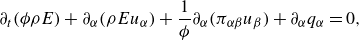 \begin{align} \partial _t ( \phi \rho E) + \partial _\alpha (\rho E u_\alpha )+ \frac {1}{ \phi } \partial _\alpha ( \pi _{\alpha \beta }u_\beta ) +\partial _{\alpha }q_{\alpha }=0, \end{align}
where the heat flux $\boldsymbol{q}$
has the following form:
$\boldsymbol{q}$
has the following form:
 \begin{align} q_{\alpha }=- \phi \lambda \partial _\alpha T - {{ \epsilon P \left ( \frac {1 }{\omega _1}- \frac {1}{2} \right ) \phi \sum _{a=1}^M H_a \partial _\alpha Y_a } }+ {\left ( \frac {\omega }{\omega _1}-1 \right ) q_\alpha ^{ {corr}}} + \left ( \frac {\omega }{\omega _1}-1 \right ) q_\alpha ^{ {diff}}, \end{align}
with the thermal conductivity $\lambda$
defined by (3.35). We now choose
$\lambda$
defined by (3.35). We now choose $q_\alpha ^{ {corr}}$
to cancel the spurious second term containing the gradient of
$q_\alpha ^{ {corr}}$
to cancel the spurious second term containing the gradient of $Y_a$
,
$Y_a$
,
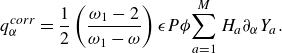 \begin{align} q_\alpha ^{ {corr}} = \frac {1}{2} \left ( \frac {\omega _1-2}{\omega _1-\omega } \right ) \epsilon P \phi {\sum _{a=1}^M H_a \partial _\alpha Y_a .} \end{align}
This is equivalent to (3.27). Finally, the inter-diffusion energy flux is introduced by choosing the last term $\boldsymbol{q}^{ {diff}}$
in (A33) as
$\boldsymbol{q}^{ {diff}}$
in (A33) as
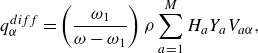 \begin{align} q_\alpha ^{ {diff}} = \left ( \frac {\omega _1}{\omega -\omega _1} \right ) \rho \sum _{a=1}^{M} H_a Y_a V_{a\alpha }, \end{align}
which is equivalent to (3.26). Substituting (A34) and (A35) into (A33), we get the heat flux $\boldsymbol{q}$
in the energy equation (A32) as a combination of the Fourier law and the inter-diffusion energy flux due to diffusion of the species (Williams Reference Williams1985; Bird et al. Reference Bird, Stewart and Lightfoot2007; Kee et al. Reference Kee, Coltrin, Glarborg and Zhu2017),
$\boldsymbol{q}$
in the energy equation (A32) as a combination of the Fourier law and the inter-diffusion energy flux due to diffusion of the species (Williams Reference Williams1985; Bird et al. Reference Bird, Stewart and Lightfoot2007; Kee et al. Reference Kee, Coltrin, Glarborg and Zhu2017),
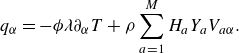 \begin{equation} {q_\alpha } = - \phi \lambda \partial _\alpha T + \rho \sum _{a=1}^{M} H_a Y_a V_{a\alpha }. \end{equation}


 Open access