A modelling framework for jet penetration into soft gels

Abstract

Jet penetration into soft gels is essential for optimising fluid delivery in medical therapies, biomedical engineering, and soft robotics. In this work, we visualise the jet flow of a Newtonian fluid into a soft viscoplastic gel using camera imaging and time-resolved tomographic particle image velocimetry (PIV) systems. The flow is primarily governed by the Reynolds number ($Re = 350-5000$) and the effective viscosity ratio ($m$ up to 22). We observe three flow regimes – mixing, jellyfish, and fingering – with transitions between them quantified in the $Re-m$ plane. An experimentally informed, systematic, practical, semi-analytical modelling framework is developed to estimate jet penetration depth over time, incorporating PIV results and an approximate functional decomposition approach to describe the velocity distribution and Reynolds stress contributions. The model provides reasonable estimations across all three regimes.

1. Introduction

The study of jets has been a long-standing area of interest, beginning with da Vinci’s foundational observations (da Vinci 1510) and advanced by Stokes (1851), Rayleigh (1878), and Reynolds (1962). These early investigations laid the groundwork for understanding jet dynamics, which continue to drive modern research into complex jet interactions with soft gels. Understanding jet penetration into soft gels (Bantawa et al. 2023; Li & Gong 2024), whose viscoplasticity endows them with the unique ability to behave as both fluids and solids (Balmforth et al. 2014; Bonn et al. 2017), is crucial for optimising fluid delivery across various fields. In medical applications, the penetration depth of jets in soft gels used as scaffolds for tissue engineering (Bailey & Appel 2024) determines the efficacy of therapeutic delivery systems (Taheri et al. 2022), including needle-free injections (Jones et al. 2019; Schoppink & Rivas 2022). Jet penetration is also essential for bio-printing (Xie et al. 2022), liquid-in-liquid printing (Bazazi et al. 2022; Xie et al. 2023), and improving precision in soft robotics for tasks such as gripping and manipulating delicate objects (Cianchetti et al. 2018). Despite these advancements, a fundamental question remains: how does jet penetration evolve over time, and to what extent can a jet penetrate a non-Newtonian soft gel upon injection?

Numerical models and velocimetry techniques, such as particle image velocimetry (PIV), have been crucial in analyzing jet dynamics in complex scenarios, including turbulent and non-Newtonian flows (Philippe et al. 2005; Pickering et al. 2021; Usta et al. 2023). PIV studies, in particular, have provided detailed insights into jet instabilities, mixing, and unsteady behaviours in various media (Davies et al. 1963; Dombrowski et al. 2005; Vessaire et al. 2020; Gauding et al. 2021; Hassanzadeh et al. 2023). Recent research, albeit focused on Newtonian fluids, also shows that fluid viscosity significantly influences jet penetration dynamics (Guyot et al. 2020). The dynamics of single-fluid viscoelastic jets have long been studied (Hosokawa et al. 2023), but research on fast jets in viscoplastic fluids – defined by yield stress and complex rheology – is still nascent and rapidly advancing (Jalaal et al. 2019). However, there is currently no model in the literature that predicts jet penetration dynamics into soft non-Newtonian materials, in particular viscoplastic ones. In this context, we conduct jet flow experiments in this study, injecting a Newtonian fluid into a soft viscoplastic gel (Balmforth et al. 2014; Thompson & Soares 2016), identifying the flow regimes, and developing an experimentally informed, simplified, semi-analytical model to estimate jet penetration depth based on PIV data.

2. Experimental setting

The jet was generated using a gear pump (ISMATEC MCP-Z Standard, 1 % accuracy) to inject fluid vertically through a centrally positioned, long cylindrical nozzle (diameter, $\hat {D}$ , of $0.432$ mm and length of 0.0508 m) into a transparent rectangular tank (20 $\times$ 10 $\times$ 10 cm $^3$ ); see figure 1. In this study, dimensionless quantities are hatless to distinguish them from the dimensional hatted quantities. The Newtonian jet fluid (dyed deionised water) was injected into a soft viscoplastic gel (transparent Carbopol solution (Carbomer 940), Making Cosmetics Co.); both were miscible and had a density of $\hat {\rho } \approx 997$ kg m $^{-3}$ , measured using a high-precision density metre (Anton Paar, DMA 35N).

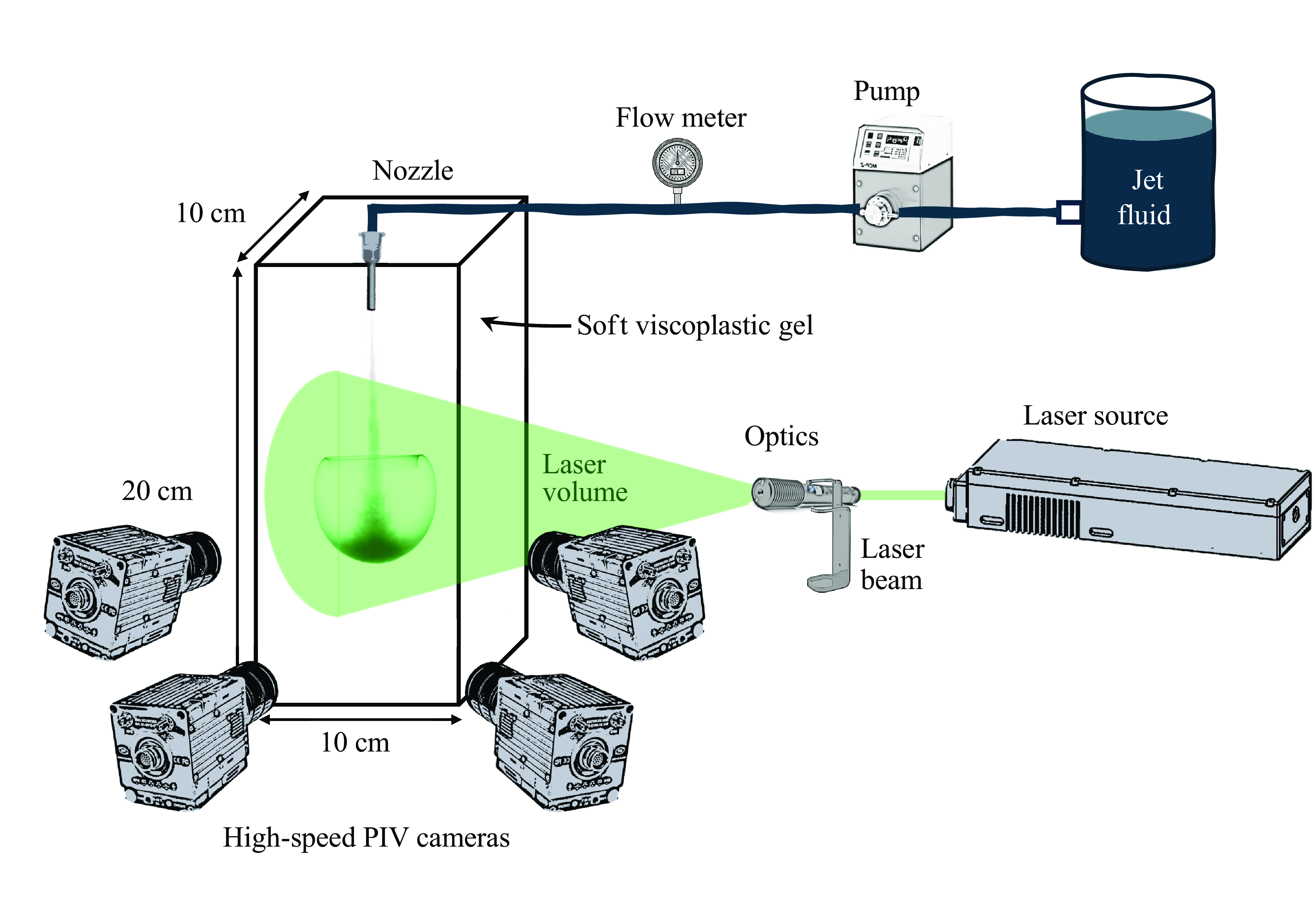
Figure 1. Schematic of experimental setup with camera imaging and PIV techniques.

The Carbopol solutions were assumed to follow the viscoplastic Herschel–Bulkley model (Balmforth et al. 2014):

(2.1) \begin{equation} \begin{cases} \hat {\tau }=\hat {\tau }_y+ \hat {\kappa }\hat {\dot {\gamma }}^n ,\hspace {5 mm} \hat {\tau }\gt \hat {\tau }_y,\\ \hat {\dot {\gamma }}=0,\hspace {16 mm} \hat {\tau }\leqslant \hat {\tau }_y, \end{cases} \end{equation}

confirmed via rheometry (DHR-3, TA Instruments). In Equation (2.1), $\hat {\tau }$ , $\hat {\dot {\gamma }}$ , $\hat {\tau }_y$ , $\hat {\kappa }$ , and $n$ represent the shear stress, shear rate, yield stress ( $0-4.3$ Pa), fluid consistency index ( $0.001-1.64$ Pa $\cdot$ s $^n$ ), and power-law index ( $0.4-1$ ), respectively. Accordingly, the effective viscosity of the ambient viscoplastic fluid is defined using the jet characteristic shear rate $ ( {\hat {V}_0}/{\hat {D}} )$ : $\hat{\mu}_{a} = {\hat \tau _y} ({{\hat V}_0}/{\hat D} )^{-1} + \hat \kappa ({{\hat V}_0}/{\hat D} )^{n - 1}$ , where the mean injection velocity ( $\hat {V}_0$ ) ranged from 0.9 m to 11 ms⁻¹, resulting in $\hat {\mu}_a$ ranging from 0.001–0.022 Pa $\cdot$ s. The jet fluid viscosity ( $\hat {\mu}_j$ ) was 0.001 Pa $\cdot$ s.

Our backlit setup, featuring light-emitting diode arrays and a digital camera (Basler acA2040–90um), captured jet flow images at 25 frames per second, which were processed using in-house codes to determine the temporal jet penetration depth. A time-resolved tomographic PIV system (LaVision) (Buzzaccaro et al. 2013; Hassanzadeh et al. 2023) analyzed the velocity fields by seeding both jet and soft gel with polyamide tracer particles (60 $\unicode{x03BC}$ m diameter, 1030 kg m $^{-3}$ density). A high-speed pulsed Nd laser (532 nm, 30 mJ per pulse) created a 5 cm laser illumination volume, with images captured by four high-speed CMOS cameras (Phantom VEO-E 340L) with 60 mm lenses (Nikon Micro Nikkor) and synchronised by a PTU-X unit. The system was calibrated with a 3D calibration plate, and 3D voxel volumes were reconstructed from particle intensity data, with velocity fields extracted via 3D cross-correlation. PIV images were processed (using DaVis 10 software) on a supercomputer (Micro Logo).

The key dimensionless numbers governing the jet flow reduce to the Reynolds number ( $Re$ ):

(2.2) \begin{equation} Re = \frac {\hat {\rho } \hat {V}_0 \hat {D}}{\hat {\mu}_j}, \end{equation}

which ranges from 350–5000, and the effective viscosity ratio ( $m$ ), obtained by balancing the characteristic viscous stresses in the jet and ambient fluids:

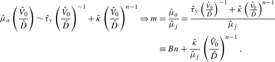(2.3) \begin{align} {\hat{\mu}_{a}} \left ( \frac {\hat V_0}{\hat D} \right ) \sim \hat \tau _y \left ( \frac {\hat V_0}{\hat D} \right )^{-1} + \hat{\kappa} \left ( \frac {\hat V_0}{\hat D} \right )^{n - 1} \Rightarrow m &= \frac {\hat{\mu}_{a}}{\hat{\mu}_{j}} = \frac {\hat \tau _y \left ( \frac {\hat V_0}{\hat D} \right )^{-1} + \hat \kappa \left ( \frac {\hat V_0}{\hat D} \right )^{n - 1}}{\hat{\mu} _{j}} \nonumber\\&\equiv Bn + \frac {\hat \kappa }{\hat{\mu}_{j}} \left ( \frac {\hat V_0}{\hat D} \right )^{n - 1}, \end{align}

where the modified Bingham number is defined as $Bn = ({\hat {\tau }_y}/{\hat {\mu}_j (\hat {V}_0 / \hat {D}))}$ , ranging from 0 to 2, and $m$ spans from 1 to 22. In other words, $m$ provides a measure of how the viscosity and yield stress effects of the ambient fluid influence the jet flow, balancing inertial and viscous forces through their Reynolds number ratios, i.e., $m \equiv {Re}/{Re^\dagger }$ , where $Re^\dagger = {\hat {\rho }\hat {V}_0\hat {D}}/{\hat {\mu}_a}$ defines the ambient fluid’s Reynolds number. Note that, as $n$ is already embedded in the definitions of both $Bn$ and $m$ , its influence as a separate parameter may be less significant. Thus, $m$ and $Re^\dagger$ mainly characterise the flow dynamics; nevertheless, they do not fully span the dimensionless space, but numerical computations, free from experimental constraints, can systematically explore their effects (Thompson & Soares 2016), a task for future work.

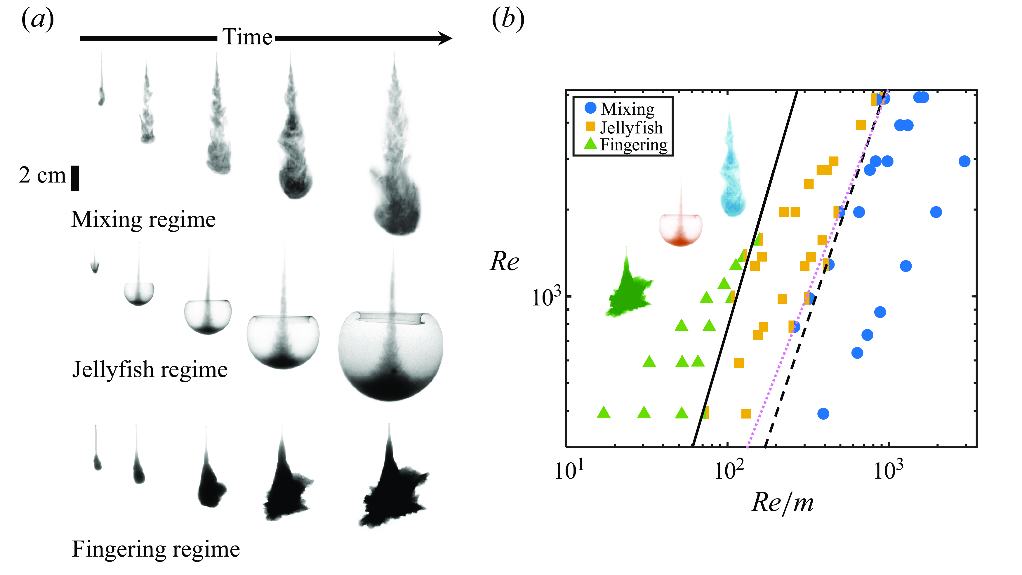
Figure 2. (a) Sequence of experimental snapshots of mixing (Re $\approx$ 1250, m $\approx$ 3), jellyfish (Re $\approx$ 1600, m $\approx$ 4), and fingering (Re $\approx$ 1000, m $\approx$ 13) regimes. Snapshots at $\hat {t} = 0.29, 0.80, 1.42, 2.65$ , and $3.18$ seconds (mixing regime, supplementary video 1); $\hat {t} = 0.63, 3.26, 5.04, 7.05$ , and $9.03$ seconds (jellyfish regime, supplementary video 2); and $\hat {t} = 0.91, 3.46, 11.91, 18.85$ , and $25.79$ seconds (fingering regime, supplementary video 3). (b) Regime classification in $Re- ({Re}/{m})$ plane, showing mixing, jellyfish, and fingering regimes, with dashed (3.1) and solid (3.2) line transition boundaries. Triangle-square and square-circle symbols mark transitions between fingering-jellyfish and jellyfish-mixing regimes, respectively. Pink dotted line represents an alternative relation using a third-order expansion of (3.1), given by $Re_c^{\textit{mixing} \to \textit{jellyfish}} = ({Re}/{m}) + ({1}/{120}) ( ({Re}/{m})^2) - ({4}/{10^6}) (({Re}/{m})^3)$ .

3. Experimental results

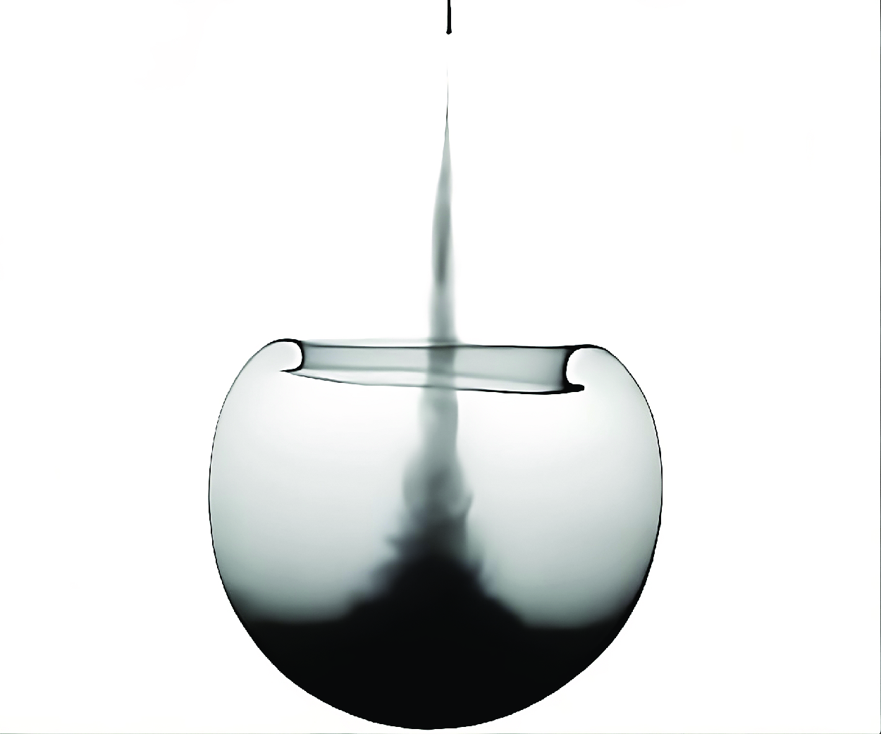
In a typical experiment (figure 2 a), dyed jet fluid is injected from a nozzle into transparent viscoplastic fluid, penetrating into it as the jet advances. The maximum axial distance reached at a given time is defined as the jet penetration depth ( $\hat {L}_p$ ). Results are presented in dimensionless form using $\hat {D}$ for lengths, $\hat {V}_0$ for velocities, and ${\hat {D}}/{\hat {V}_0}$ for times, unless otherwise stated. Our results reveal the existence of three regimes: mixing, jellyfish, and fingering. The upper row of figure 2(a) shows the mixing regime, which occurs at high $Re$ and low $m$ , where significant mixing between the jet and soft gel is observed, along with an initial stable region. At higher $m$ and lower $Re$ , the middle row illustrates the jellyfish regime, i.e., a newly identified flow state, reported for the first time in viscoplastic fluids, and characterised by a vortex ring around the jet tip caused by instabilities. This vortex grows, and the jet radius expands transversely due to the higher $m$ . With further increases in $m$ and decreases in $Re$ , the lower row shows the fingering regime, where the jet fluid initially penetrates the yield-stress fluid before becoming trapped (Hassanzadeh et al. 2023), eventually forming evolving fingers. Moreover, our PIV analysis reveals fluctuations within each regime, with an average fluctuation intensity – defined as the ratio of turbulent to total kinetic energy – at $y \approx 40$ of approximately 60 %, 30 %, and 55 % for the mixing, jellyfish, and fingering regimes, respectively.

As shown in figure 2(b), the three morphological regimes – mixing, jellyfish, and fingering – can be classified using $Re$ and $m$ . Here, the transition from mixing (at high $Re^\dagger$ ) to jellyfish, and then to fingering (as $Re^\dagger$ decreases), is influenced by a combination of inertial and effective viscous forces. The critical transition between the mixing and jellyfish regimes is given by:

(3.1) \begin{equation} Re_c^{\textit {mixing} \to \textit {jellyfish}} = 200\;m \left (m-1\right ), \;\;\; 1\lesssim m\lesssim 22,\,\,\,O(10^2)\lesssim Re \lesssim O(10^4). \end{equation}

While the simplified relation in (3.1) provides a convenient approximation, a more precise transition can be obtained through higher-order expansions, as shown by the dotted line ( $Re_c^{\textit {mixing} \to \textrm {jellyfish}} = ({Re}/{m}) + ({1}/{120}) ( ({Re}/{m})^2) - ({4}/{10^6}) ( ({Re}/{m})^3)$ ) in figure 2(b).

The fingering regime emerges as $m$ increases, particularly with higher yield stress in the soft gel. The critical transition Reynolds number between the jellyfish and fingering regime is given by:

(3.2) \begin{equation} Re_c^{\kern1pt \textit {jellyfish} \to \textit {fingering}} = 15\;m \left (m-1\right ), \;\;\; 1\lesssim m\lesssim 22,\,\,\,O(10^2)\lesssim Re \lesssim O(10^4). \end{equation}

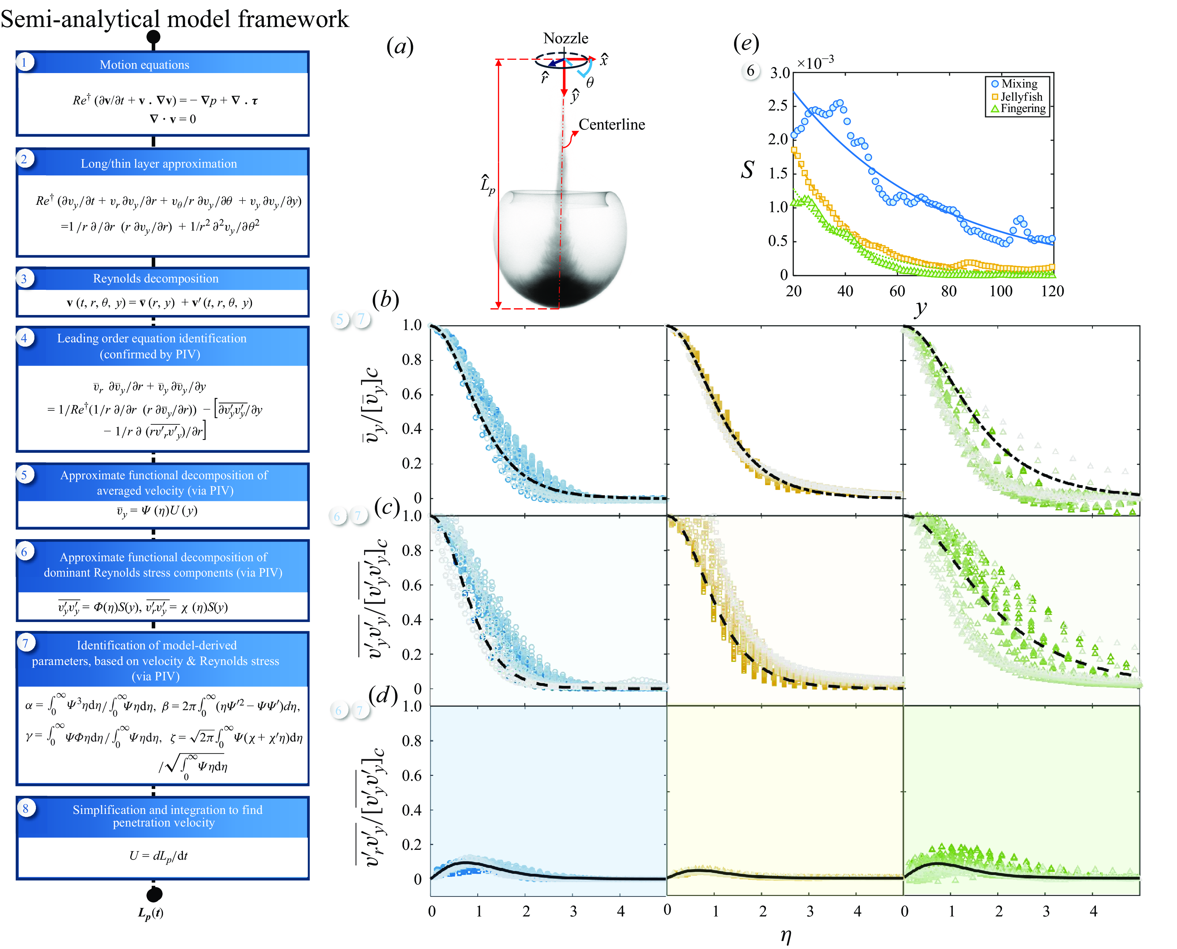
Figure 3. Modelling framework and results: (a) Newtonian jet injection into a viscoplastic fluid, showing jet centreline (dashed-dot), coordinates, and penetration depth ( $\hat {L}_p$ ) at $Re \approx 1000$ and $m \approx 4.5$ . Normalised axial velocity (b), axial Reynolds stress (c), and radial-axial Reynolds stress (d) versus $\eta$ at different axial distances, with brighter symbols indicating greater distances ( $30 \lesssim y \lesssim 100$ ). Each row corresponds to mixing, jellyfish, and fingering regimes (left to right). Fitted velocity curves (dashed-dotted) are $\cosh (\eta )^{-1.539}$ (mixing), $\cosh (\eta )^{-1.300}$ (jellyfish), and $\cosh (\eta )^{-0.864}$ (fingering), consistent with (Pope 2000). Fitted axial Reynolds stress curves (dashed) are $\cosh (\eta )^{-2.226}$ , $\cosh (\eta )^{-1.594}$ , and $\cosh (\eta )^{-0.623}$ , and fitted radial-axial Reynolds stress curves (solid) are $0.22\sinh (\eta )\cosh (\eta )^{-2.5}$ , $0.12\sinh (\eta )\cosh (\eta )^{-3}$ , and $0.2\sinh (\eta )\cosh (\eta )^{-2.6}$ for the respective regimes. Mean squared errors between fitted and measured velocity profiles are $0.38\,\%$ (mixing), $0.08\,\%$ (jellyfish), $4.47\,\%$ (fingering), with Reynolds stress errors in a comparable range. (e) $S(y)$ , versus $y$ , with fitted curves $0.0039e^{-0.018y}$ (solid), $0.0044e^{-0.043y}$ (dashed), and $0.0031e^{-0.045y}$ (dotted).

4. Model development and comparison with experiments

We develop an experimentally guided, semi-analytical model to estimate the jet penetration depth into the soft gel over time. The model is based on dimensionless motion equations for momentum and continuity in a cylindrical coordinate system (with $(r, \theta , y)$ denoting radial, tangential, and axial directions; see figure 3 a):

(4.1) \begin{align} Re^\dagger \left ( {\frac {{\partial \mathbf{{v}}}}{{\partial t}} + \mathbf{{v}} \cdot \nabla \mathbf{{v}}} \right ) &= - \nabla p + \nabla \cdot \boldsymbol{\tau }, \end{align}

(4.2) \begin{align} \nabla \cdot \mathbf{v}&=0, \end{align}

where $\mathbf{{v}} = (v_r, v_\theta , v_y )$ represents the velocity field, $p$ the pressure, and $\boldsymbol{\tau }$ the stress tensor. Using $Re^\dagger$ in (4.1) simplifies the analysis by encapsulating the viscoplastic fluid’s rheology into an effective viscosity, reflecting the dominant inertial-to-viscous force ratio. This approach captures the gel’s resistance properties, governed by its yield stress and characteristic shear rate, which critically influence the jet penetration depth and flow morphology. While it aligns with the observed flow transitions (mixing, jellyfish, and fingering, as shown in figure 2 b), it neglects local variations in viscosity, detailed mixing mechanisms, and secondary flow dynamics, such as vortex and finger formation.

We assume that the jet dynamics develop over a thin, elongated layer with thickness $\zeta$ and length $\ell$ . This allows us to define an arbitrary small aspect ratio $\varepsilon = \zeta /\ell$ , and we rescale our variables as follows:

(4.3) \begin{equation} \varepsilon y = {y^*}\,\,, \varepsilon t = {t^*}\,\,,\varepsilon p = {p^ * }\,\,,{v_r} = \varepsilon v_r^*\,\,,{v_\theta } = \varepsilon v_\theta ^*. \end{equation}

Therefore, the motion equations in the leading order can be found as:

(4.4) \begin{align} &\qquad\qquad\qquad\qquad O\big ( {R{e^\dagger }{\varepsilon ^3}} \big ) = - \frac {{\partial {p^*}}}{{\partial r}} + O\big ( {{\varepsilon ^2}} \big ), \end{align}

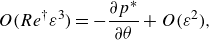(4.5) \begin{align} &\qquad\qquad\qquad\qquad O\big ( {R{e^\dagger }{\varepsilon ^3}} \big ) = - \frac {{\partial {p^*}}}{{\partial \theta }} + O\big ( {{\varepsilon ^2}} \big ), \end{align}

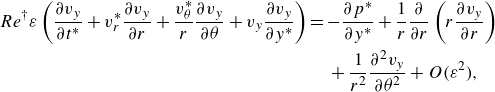(4.6) \begin{align} &R{e^\dagger }\varepsilon \left ( {\frac {{\partial {v_y}}}{{\partial {t^*}}} + v_r^*\frac {{\partial {v_y}}}{{\partial r}} + \frac {{v_\theta ^*}}{r}\frac {{\partial {v_y}}}{{\partial \theta }} + {v_y}\frac {{\partial {v_y}}}{{\partial {y^*}}}} \right ) = - \frac {{\partial {p^*}}}{{\partial {y^*}}} + \frac {1}{r}\frac {\partial }{{\partial r}}\left ( {r\frac {\partial v_y }{{\partial r}}} \right ) \nonumber\\&\qquad\qquad\qquad\qquad\qquad\qquad\qquad\qquad\qquad\,\, + \frac {1}{{{r^2}}}\frac {{{\partial ^2}{v_y}}}{{\partial {\theta ^2}}} + O\big ( {{\varepsilon ^2}} \big ), \end{align}

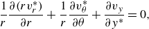(4.7) \begin{align} &\qquad\qquad\qquad\qquad \frac {1}{r}\frac {{\partial (rv_r^*)}}{{\partial r}} + \frac {1}{r}\frac {{\partial v_\theta ^*}}{{\partial \theta }} + \frac {{\partial {v_y}}}{{\partial {y^*}}} = 0, \end{align}

which, considering $\varepsilon \ll 1$ with a fixed $\varepsilon Re^\dagger$ (implying $Re^\dagger \propto {1}/{\varepsilon } \gg 1$ ), leads to the following axial momentum equation:

(4.8) \begin{equation} R{e^\dagger }\varepsilon \left ( {\frac {{\partial {v_y}}}{{\partial {t^*}}} + v_r^*\frac {{\partial {v_y}}}{{\partial r}} + \frac {{v_\theta ^*}}{r}\frac {{\partial {v_y}}}{{\partial \theta }} + {v_y}\frac {{\partial {v_y}}}{{\partial {y^*}}}} \right ) = - \frac {{\partial {p^*}}}{{\partial {y^*}}} + \frac {1}{r}\frac {\partial }{{\partial r}}\left ( {r\frac {\partial v_y }{{\partial r}}} \right ) + \frac {1}{{{r^2}}}\frac {{{\partial ^2}{v_y}}}{{\partial {\theta ^2}}}, \end{equation}

where $p^*=p^*(y)$ only. Now, it can be transformed back to the original variable scaling to reach:

(4.9) \begin{equation} Re^\dagger \left ({\frac {{\partial v_y}}{{\partial {t}}} + {v_r}\frac {{\partial v_y}}{{\partial r}} + \frac {{v_\theta }}{r}\frac {{\partial v_y}}{{\partial \theta }} + v_y\frac {{\partial v_y}}{{\partial {y}}}} \right ){\textrm { }} = \frac {1}{r}\frac {\partial }{{\partial r}}\left ( {r\frac {\partial v_y }{{\partial r}}} \right ) + \frac {1}{{{r^2}}}\frac {{{\partial ^2}v_y}}{{\partial {\theta ^2}}}, \end{equation}

in which the pressure gradient term is neglected, following the fact that pressure does not depend on $r$ and pressure is constant at larger radial distances from the jet centreline, in line with the literature (Guimarães et al. 2023). Also, this is due to the dominance of inertial and viscous forces, as the gel’s yield stress and viscosity primarily govern penetration depth and morphology.

We now derive the Reynolds-averaged form of (4.9), by decomposing the velocity into its mean (bar notation) and fluctuating (prime notation) components in the form of:

(4.10) \begin{equation} \mathbf{{v}}\left ( {t,r,\theta ,y} \right ) = {\overline {\mathbf{v}}}\left ( {r,y} \right ) + \mathbf{{v}'}\left ( {t,r,\theta ,y} \right ), \end{equation}

where the overbar denotes circumferential and ensemble averaging, resulting in the following leading order motion equations:

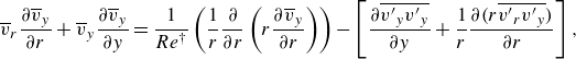(4.11) \begin{align} &{\overline v_r}\frac {{\partial {{\overline v}_y}}}{{\partial r}} + {\overline v_y}\frac {{\partial {{\overline v}_y}}}{{\partial y}} = \frac {1}{{Re^\dagger }}\left ( \frac {1}{r}\frac {\partial }{{\partial r}}\left ( {r\frac {\partial \overline {v}_y }{{\partial r}}} \right ) \right ) - \left [ {\frac {{\partial \overline {{{v'}_y}{{v'}_y}} }}{{\partial y}} + \frac {1}{r}\frac {\partial \big (r \overline {{{v'}_r}{{v'}_y}}\big )}{\partial r} } \right ], \end{align}

(4.12) \begin{align} &\qquad\qquad\qquad\qquad\qquad \frac {1}{r}\frac {{\partial \left (r{{\overline v}_r}\right )}}{{\partial r}} + \frac {{\partial {{\overline v}_y}}}{{\partial y}}{\textrm { }} = 0, \end{align}

where $\overline {{v'}_y {v'}_y}$ and $\overline { {v'}_r {v'}_y}$ are dominant Reynolds stresses (confirmed by PIV), and the flow is assumed to be statistically steady.

As shown in figure 3(b–d), the profiles of ${\overline {v}_y}/{(\overline {v}_y)_c}$ , $ {\overline {v'_y v'_y}}/{(\overline {v'_y v'_y})_c}$ and ${\overline {v'_r v'_y}}/{(\overline {v'_y v'_y})_c}$ (with the subscript $c$ denoting the centreline) exhibit an approximate scaling behaviour, with the scaling variable defined as:

(4.13) \begin{equation} \eta = \frac {r}{r_{1/2}}, \end{equation}

in which $r_{1/2}(y)$ represents the radial distance from the centreline where the mean velocity drops to half of its centreline value, characterising the jet’s lateral spread (Pope 2000; Kuhn et al. 2021). Note that, although dispersions and deviations from a universal scaling collapse are observed, particularly in the fingering regime (figure 3 e), where localised stress effects and flow confinement introduce variations in the velocity profile, our assumed approximate scaling captures the dominant trends and serves as a practical approximation for a simplified model. Thus, a degree of dependence on $\eta$ allows the mean velocity, $\overline {v}_y$ , to be approximately expressed via a functional decomposition:

(4.14) \begin{equation} \overline {v}_y = U(y) \Psi (\eta ), \end{equation}

where $\Psi (\eta )$ is found for a representative experiment in each regime via PIV data fitting (figure 3 b). Similarly, for the dominant Reynolds stress terms, we write:

(4.15) \begin{equation} \overline {{v}'_y{v}'_y} = {S}({y})\Phi ({\eta }), \,\,\,\,\, \overline {{v}'_r{v}'_y} = {S}({y})\chi ({\eta }), \end{equation}

where ${S}({y})$ , $\Phi ({\eta })$ , and $\chi (\eta )$ are found for each regime via PIV data fitting (figure 3 c–e).

Multiplying the Equation (4.11) by $\overline {v}_y$ and integrating it over volume gives:

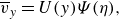
(4.16) \begin{align} &\int _0^y {\int _0^\infty {\left ( {{{\overline v }_r}{{\overline v }_y}\frac {{\partial {{\overline v }_y}}}{{\partial r}} + \overline v _y^2\frac {{\partial {{\overline v }_y}}}{{\partial \mathsf{y}}}} \right )} } 2\pi r{\textrm d}r{\textrm d}\mathsf{y} = \nonumber \\ &\int _0^y {\int _0^\infty {\left [ {\frac {1}{{Re^\dagger }}\left ( {{{\overline v }_y}\frac {{{\partial ^2}{{\overline v }_y}}}{{\partial {r^2}}} + \frac {{{{\overline v }_y}}}{r}\frac {{\partial {{\overline v }_y}}}{{\partial r}}} \right ) - {{\overline v }_y}\frac {{\partial \overline {{{v}^{\prime}_y}{{v}^{\prime}_y}} }}{{\partial \mathsf{y}}}} - \frac {{\overline v }_y}{r}\frac {\partial \left (r \overline {{{v}^{\prime}_r}{{v}^{\prime}_y}}\right )}{\partial r}\right ]}} 2\pi r{\textrm d}r{\textrm d}\mathsf{y}, \end{align}

where $\mathsf{y}$ the dummy variable of integration. Using the continuity equation, the left-hand side of (4.16) is reformulated. The term $\overline {v}_y ({\partial ^2 \overline {v}_y}/{\partial r^2})$ is decomposed as ${1}/{2} ({\partial ^2 (\overline {v}_y^2)}/\def\luminalatbreak{} {\partial r^2}) - (({\partial \overline {v}_y}/{\partial r} )^2)$ ; the first component, contributing only $\sim$ 7 % across all regimes based on the PIV results, is neglected, yielding a simplified expression after some algebra:

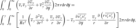
(4.17) \begin{align} \frac {3}{2}\int _0^y \def\negativespace{}\def\negativespace{}{\int _0^\infty {\bar v_y^2} } \frac {{\partial {{\bar v}_y}}}{{\partial \mathsf{y}}}2\pi r\textrm{d}r\textrm{d}\mathsf{y} & = \frac {1}{{Re^{\dagger }}}\left [ {\int _0^y \def\negativespace{}\def\negativespace{}{\int _0^\infty {{{\bar v}_y}} } \frac {{\partial {{\bar v}_y}}}{{\partial r}}2\pi \textrm{d}r\textrm{d}\mathsf{y} - \int _0^y \def\negativespace{}\def\negativespace{}{\int _0^\infty \def\negativespace{}{{{\left (\def\negativespace{} {\frac {{\partial {{\bar v}_y}}}{{\partial r}}}\def\negativespace{} \right )}^2}} } 2\pi r\textrm{d}r\textrm{d}\mathsf{y}} \def\negativespace{}\right ] \notag \\&\quad - \int _0^y {\int _0^\infty {{{\bar v}_y} {\frac {{\partial \overline {{{v'}_y}{{v'}_y}} }}{{\partial \mathsf{y}}}}} } 2\pi r\textrm{d}r\textrm{d}\mathsf{y} \nonumber \\ & \quad - \int _0^y {\int _0^\infty \frac {{\overline v }_y}{r}\frac {\partial \left (r \overline {{{v'}_r}{{v'}_y}}\right )}{\partial r} } 2\pi r\textrm{d}r\textrm{d}\mathsf{y}. \end{align}

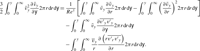
Subsequently, using the approximate functional decomposition approach ((4.13), (4.14), and (4.15)), along with integration by parts gives:

(4.18) \begin{align} &\frac {1}{2}\left [ {{U^3} {r_{1/2}^2} \int _0^\infty {{\Psi ^3}} 2\pi \eta {\textrm d}\eta -U^3(0) {r_{1/2}^2}(0) \int _0^\infty {{\Psi ^3}} 2\pi \eta {\textrm d}\eta } \right ] \notag \\ & = \frac {1}{{Re^{\dagger }}}\left [ {\int _0^y {\int _0^\infty {{U^2}} } \Psi \Psi '2\pi \textrm{d}\eta \textrm{d}\mathsf{y} - \int _0^y {\int _0^\infty {{U^2}} } {{\Psi '}^2}2\pi \eta {\textrm d}\eta {\textrm d}\mathsf{y}} \right ] \notag \\ &\quad - \int _0^y {\int _0^\infty U {r_{1/2}^2}} \Psi S' \Phi 2\pi \eta \textrm{d}\eta \textrm{d}\mathsf{y} - \int _0^y {\int _0^\infty U {r_{1/2}} } \Psi S \left (\chi + \chi ' \eta \right )2\pi \textrm{d}\eta \textrm{d}\mathsf{y}, \end{align}

Now, multiplying and dividing (4.18) by $\int _{0}^{\infty } \Psi 2 \pi {\eta } {\textrm d}{\eta }$ , isolating the jet flux ( $Q$ ), and applying the boundary condition ( $U(0)=1$ ), we eventually arrive at:

(4.19) \begin{equation} \frac {1}{2}\alpha Q \left ( {{U^2} - 1} \right ) = -\frac {1}{{Re^\dagger }}\int _0^y {{U^2}\beta \textrm{d}\mathsf{y}} - \int _0^y {QS'\gamma \textrm{d}\mathsf{y}}- \int _0^y {\sqrt {QU}S \zeta \textrm{d}\mathsf{y}}, \end{equation}

where the prime denotes the derivative and the model-derived parameters $\alpha$ , $\beta$ , $\gamma$ , and $\zeta$ are functions of the jet velocity and Reynolds stress profiles:

(4.20) \begin{equation} \left \{ {\begin{array}{*{20}{l}} {\alpha = \dfrac {{\int _0^\infty {{\Psi ^3}} \eta {\textrm d}\eta }}{{\int _0^\infty \Psi \eta {\textrm d}\eta }},}\\[6pt] {\beta = 2\pi \int _0^\infty {\left ( {\eta {{\Psi '}^2} - \Psi \Psi '} \right ){\textrm d}\eta } ,}\\[6pt] {\gamma = \dfrac {{\int _0^\infty \Psi \Phi \eta {\textrm d}\eta }}{{\int _0^\infty \Psi \eta {\textrm d}\eta }},}\\[6pt] {\zeta = \sqrt {2\pi } \dfrac {{\int _0^\infty \Psi \left (\chi + \chi ' \eta \right ) {\textrm d}\eta }}{\sqrt {\int _0^\infty \Psi \eta {\textrm d}\eta }}.} \end{array}} \right . \end{equation}

In (4.19), $Q= {U} r^2_{1/2} \int _{0}^{\infty } 2 \pi \eta \Psi {\textrm d}\eta = Q_0 + Q_e$ , where $Q_0$ is the injection flux and $Q_e$ accounts for entrainment, with PIV analysis showing $Q_e$ contributes 23–30 % across regimes. However, for simplicity and analytical tractability, we assume $Q \approx Q_0=\pi /4$ (constant), acknowledging a jet momentum underestimation. Also, since the last term in (4.19) (radial-axial Reynolds stress contribution) has a secondary effect on axial momentum transport, with PIV measurements showing its impact is 4–15 % of dominant terms across regimes, we omit it for simplicity.

Taking the derivative of (4.19) with respect to $y$ , integrating, and applying the boundary condition $U(0) = 1$ yield an analytical expression for the jet velocity:

(4.21) \begin{equation} U(y) = {\left ( {1 - \frac {{2\gamma }}{\alpha }\int _0^y {\exp \left ( {\frac {{2\beta \mathsf{y}}}{{\alpha Q_0Re^\dagger }}} \right )S'{\textrm d}\mathsf{y}} } \right )^{\frac {1}{2}}}\exp \left ( { - \frac {{\beta y}}{{\alpha Q_0Re^\dagger }}} \right ), \end{equation}

which is then integrated (via ${U} = ({{\textrm d}{L_p}}/{{\textrm d}{t}})$ ) to calculate the jet penetration depth ( $L_p$ ) as a function of time. We can, thus, derive the variation in the jet penetration depth over time based on the key parameters such as the jet velocity profiles, dominant Reynolds stress, injection velocity, and flow rate. Figure 3(b) show the jet velocity profiles used in our model, with $\alpha$ values of 0.25, 0.24, and 0.20, and $\beta$ values of 5.8, 5.7, and 5.4 for the mixing, jellyfish, and fingering regimes, respectively. The Reynolds stress profiles are detailed in figures 3(c) and 3(d), yielding $\gamma$ values of 0.32, 0.35, and 0.41, for the respective regimes. According to our PIV analysis for different cases, $\alpha$ , $\beta$ , and $\gamma$ vary by up to $\pm$ 8 %.

The profiles for $\Psi (\eta )$ , $\Phi (\eta )$ , $S(y)$ are extracted from PIV data and assumed constant within each flow regime (mixing, jellyfish, fingering). Model-derived parameters $\alpha$ , $\beta$ , and $\gamma$ encapsulate the axial velocity dynamics and interactions with Reynolds stresses, while $S(y)$ reflects axial decay, energy dissipation, and turbulence damping. These parameters, assumed applicable without re-fitting for each experiment, enable efficient estimation of $L_p$ over time. This provides a robust, validated approach, while simplifying analysis and enhancing scalability across experimental scenarios.

Figure 4. (a) Jet penetration depth over time for experiments (symbols) and model (lines) across three flow regimes: mixing ( $Re \approx 1300$ , $m\approx 1$ , blue), jellyfish ( $Re \approx 1300$ , $m\approx 4$ , red), and fingering ( $Re \approx 1300$ , $m\approx 11$ , green). (b) Model versus experimental results of $L_p$ at $t\approx O(10^3)$ , both multiplied by $Re$ to illustrate the data spread. The solid line shows $\hat {L}^{\textit{Model}}_p = \hat {L}^{\textit{Experiment}}_p$ . Data points’ face colour, size, and edge width indicate $Re$ , $m$ , and $Bn$ , with circles, squares, and triangles for mixing, jellyfish, and fingering regimes. Inset shows model outputs vs. experimental results of $\hat {L}_{p}$ (dimensional) from $\hat {t} = 0.4$ s to the experiment end, with black/red edges for start/end points and dashed lines for time variation.

Figure 4(a) compares the model’s outputs with experimental data across the three flow regimes, applying the obtained values of $\alpha$ , $\beta$ , and $\gamma$ to all cases with similar flow regimes. The model demonstrates reasonable estimations of the jet penetration depth over time, even in the challenging fingering regime with high yield stress. In the mixing regime, the model closely aligns with experimental values initially, with mid-time deviations converging later as energy dissipation is accounted for. In the jellyfish regime, the model initially overestimates the penetration depth but eventually aligns with experimental trends by the end of the injection period. The inset in figure 4(b) shows the variation of $\hat {L}_p$ between the model and experimental data, with initial overestimations likely due to unaccounted losses near the nozzle exit. This discrepancy is somewhat corrected over time, although occasional underestimations can also occur. The model’s accuracy generally improves over time across all flow regimes, although higher $Re$ values result in greater deviations, possibly due to underestimated Reynolds stresses. For a larger dataset, the main panel in figure 4(b) demonstrates the model’s overall estimative capability but also indicates increasing deviations at higher $Re$ .

5. Conclusions

A Newtonian jet penetrating a soft viscoplastic gel was studied across viscosity ratios from 1 to 22 and Reynolds numbers between 350 and 5000. Our experiments identified three distinct responses of the viscoplastic fluid: a mixing regime dominated by turbulence, a jellyfish regime with vortex formation and radial jet expansion, and a fingering regime where the jet becomes confined and forms localised fingers. To estimate the penetration depth over time, we developed an experimentally informed semi-analytical model incorporating key dimensionless parameters, such as effective viscosity and Reynolds stresses, and leveraging an approximate scaling approach. The model demonstrates reasonable estimations across all regimes, providing a robust framework for understanding jet interactions with soft viscoplastic gels. However, it does not account for long-term effects, such as dominant mixing or extensive finger formation, where nonlinearities and instabilities become significant. Future work should address these complexities to extend the model’s applicability to high-yield-stress environments and more intricate scenarios. Finally, we investigated the problem in $Re-m$ space, and future work incorporating other dimensionless groups, such as the Bingham number and power-law index, could enhance understanding of our jet flows.