


1. Introduction
Flow control and optimisation has long been a fundamental area of research in fluid mechanics (Brunton & Noack Reference Brunton and Noack2015; Fukagata et al. Reference Fukagata, Iwamoto and Hasegawa2024; Vinuesa Reference Vinuesa2024), driven by the need to reduce drag and regulate heat transfer in engineering applications. From aerospace to automotive systems, as well as energy and process industries, controlling the flow in a manner that optimises performance can significantly improve efficiency and reduce operational costs. Traditional methods of flow control are typically categorised into passive and active approaches. Passive methods, such as riblets (García-Mayoral & Jiménez Reference García-Mayoral and Jiménez2011), surface roughness (Yang et al. 2023), or porous media (Rosti et al. Reference Rosti, Cortelezzi and Quadrio2015; Wang et al. Reference Wang, Chu, Lozano-Durán, Helmig and Weigand2021a , Reference Wang, Yang, Evrim, Terzis, Helmig and Chu2021b , Reference Wang, Lozano-Durán, Helmig and Chu2022), alter the flow in a fixed manner without requiring external energy. While passive strategies are effective in certain scenarios, they are limited by their inability to adapt to changing flow conditions. Active flow control, by contrast, provides dynamic manipulation of the flow-through external actuators, allowing for more flexibility in achieving desired flow behaviours. An example of active control often referenced is opposition control (Choi et al. Reference Choi, Moin and Kim1994; Bewley et al. Reference Bewley, Moin and Temam2001; Kametani & Fukagata Reference Kametani and Fukagata2011), which involves implementing local wall blowing and suction to negate the fluctuations in wall-normal velocity at a specific height from the wall. Wang et al. (Reference Wang, Atzori and Vinuesa2024) performed high-resolution large-eddy simulations to evaluate opposition control for turbulent boundary layers on wing surfaces, analysing drag reduction and turbulence dynamics under adverse pressure gradients. Their findings highlight that its effectiveness in reducing friction drag is challenged by increased wall-normal convection from stronger gradients, especially in complex geometries such as those found in wing applications.
In the compressible regime, flow control and optimisation become even more critical, as the aerodynamic and thermal challenges intensify with increasing Mach numbers. Kametani et al. (Reference Kametani, Kotake, Fukagata and Tokugawa2017) investigated the drag reduction capabilities of uniform blowing in supersonic wall-bounded turbulent flows, concluding that Mach number dependence primarily stems from varying thermal properties such as density and temperature, similar to the effect of Mach number on turbulent statistics in uncontrolled flows. Yao & Hussain (Reference Yao and Hussain2021) achieved a maximal drag reduction of 23 % with opposition control in a turbulent channel flow at Mach numbers $M_b = 1.5$
.
$M_b = 1.5$
.
Another promising approach involves the use of porous media. In compressible turbulent flows, porous surfaces are particularly effective for managing thermal loads, enhancing heat transfer in thermal protection systems, which makes them highly relevant for aerospace applications. These techniques offer significant potential for improving both aerodynamic performance and thermal management in high-speed compressible flows. Recent experimental and numerical studies have demonstrated that by tuning the permeability of the porous medium, it is possible to achieve significant modulation of both turbulence intensity and drag, providing an approach to drag reduction in practical applications (Manes et al. Reference Manes, Pokrajac, McEwan and Nikora2009; Kim et al. Reference Kim, Blois, Best and Christensen2018; Rosti et al. Reference Rosti, Brandt and Pinelli2018; Gómez-de Segura & García-Mayoral Reference Gómez-de-Segura and García-Mayoral2019; Lācis et al. Reference Lācis, Sudhakar, Pasche and Bagheri2020; Chu et al. Reference Chu, Wang, Yang, Terzis, Helmig and Weigand2021). For instance, in thermal protection systems (TPS) used in high-speed aerospace applications (Mansour et al. Reference Mansour, Panerai, Lachaud and Magin2024), effective flow control can significantly reduce heat loads and improve material longevity, ensuring better thermal management and structural integrity. Chen & Scalo (Reference Chen and Scalo2021a
) studied flows in channels at Mach numbers of $M_b = 1.5$
and
$M_b = 1.5$
and $M_b = 3.5$
, where the channel walls were modelled using a time-domain impedance boundary condition (Chen & Scalo Reference Chen and Scalo2021a
,
Reference Chen and Scalob
). Large-eddy simulations were employed to examine how porous walls influence the flow, particularly with respect to pressure changes and stress distribution. These findings highlight the potential of porous media in advancing the design of efficient flow systems, offering enhanced control over turbulent structures and contributing to both aerodynamic performance and thermal regulation.
$M_b = 3.5$
, where the channel walls were modelled using a time-domain impedance boundary condition (Chen & Scalo Reference Chen and Scalo2021a
,
Reference Chen and Scalob
). Large-eddy simulations were employed to examine how porous walls influence the flow, particularly with respect to pressure changes and stress distribution. These findings highlight the potential of porous media in advancing the design of efficient flow systems, offering enhanced control over turbulent structures and contributing to both aerodynamic performance and thermal regulation.
While traditional flow optimisation and control methods have demonstrated effectiveness in specific scenarios, they often rely on empirically tuned parameters. To address these challenges, the field has increasingly turned to advanced control and optimisation techniques that provide a more systematic and rigorous approach. Among these, adjoint-based optimisation has become a cornerstone in the pursuit of efficient flow control and design, offering a mathematically robust framework for optimising performance across a wide range of flow configurations (Kungurtsev & Juniper Reference Kungurtsev and Juniper2019) or data assimilation (Plogmann et al. Reference Plogmann, Brenner and Jenny2024). The adjoint method allows the efficient computation of gradients of an objective function, such as drag, lift, heat transfer or energy dissipation, with respect to a large number of control variables by solving the adjoint equations derived from the governing Navier–Stokes equations. This approach is particularly advantageous because the cost of computing the gradient is independent of the number of design parameters, making it highly suitable for complex systems, such as aerodynamic shape optimisation, where traditional optimisation techniques would be prohibitively expensive (Jameson Reference Jameson1988). Adjoint-based techniques have been successfully applied to a wide range of flow control problems, including boundary layer manipulation, turbulence suppression and noise reduction (Bewley et al. Reference Bewley, Moin and Temam2001; Kim Reference Kim2003).
Despite its strengths, adjoint optimisation faces several challenges. One of the primary difficulties lies in the derivation and implementation of the adjoint equations. For these complex flows, the adjoint equations must be accurately formulated and solved in tandem with the primal equations, leading to significant numerical complexity and computational expense. Additionally, the presence of discontinuities in the flow, such as shock waves or regions of flow separation, can lead to difficulties in ensuring stable and convergent adjoint solutions, as these sharp gradients are challenging to resolve in both the forward and adjoint simulations (Giles & Pierce Reference Giles and Pierce2000). Furthermore, adjoint-based methods are often limited by the need for accurate linearisation of complex physical models, and the derivation of adjoint systems for industrial-scale solvers can be time consuming and error prone. Moreover, adjoint methods can struggle with handling non-smooth optimisation landscapes, particularly in turbulent or chaotic flow regimes (Vishnampet et al. Reference Vishnampet, Bodony and Freund2015), where the adjoint variables exhibit high sensitivity to small changes in the control inputs, leading to slow convergence or even divergence in optimisation.
Machine learning (ML) has also emerged as a promising avenue for fluid mechanics (Duraisamy et al. Reference Duraisamy, Iaccarino and Xiao2019; Srinivasan et al. Reference Srinivasan, Guastoni, Azizpour, Schlatter and Vinuesa2019; Vinuesa & Brunton Reference Vinuesa and Brunton2022; Chu & Pandey Reference Chu and Pandey2024; Han et al. Reference Han, Huang and Xu2024; Yang et al. Reference Yang, Xu, Tian, Guo, Wu and Chu2024). Bayesian optimisation (BO), in particular, is suited for cases where objective function evaluations are expensive, as it uses probabilistic models to identify promising regions of the control space. This method has been used to optimise flow control strategies in scenarios where traditional gradient-based methods may struggle, offering a more global search that accounts for uncertainty in the control space. Mahfoze et al. (Reference Mahfoze, Moody, Wynn, Whalley and Laizet2019) developed a BO framework to optimise low-amplitude wall-normal blowing control in a turbulent boundary layer flow. The BO framework identifies the optimal blowing amplitude and coverage, achieving up to a 5 % net power savings within 20 optimisation iterations, which require 20 direct numerical simulations (DNS). Reinforcement learning (RL), on the other hand, has been increasingly explored for flow control applications where the control strategy can be learned through interaction with the flow environment (Sonoda et al. Reference Sonoda, Liu, Itoh and Hasegawa2023). Reinforcement learning algorithms allow for agents to learn optimal control policies through trial and error. In the context of flow control, RL has demonstrated potential in complex, nonlinear flow configurations, where direct gradient methods may not provide effective solutions.
In addition to adjoint methods and ML, differentiable fluid dynamics combines the strengths of traditional gradient-based methods with the flexibility of ML frameworks. In differentiable fluid dynamics, the entire fluid simulation becomes differentiable, allowing the efficient computation of control parameter gradients using automatic differentiation (AD) (Kochkov et al. Reference Kochkov, Smith, Alieva, Wang, Brenner and Hoyer2021; List et al. Reference List, Chen and Thuerey2022). The early development of AD in scientific computing predates the ML era (Griewank & Walther Reference Griewank and Walther2008). In the area of optimisation design, AD has been incorporated into the development of the discrete adjoint (Albring et al. Reference Albring, Sagebaum and Gauger2016; Bombardieri et al. Reference Bombardieri, Cavallaro, Sanchez and Gauger2021), providing an automated method for generating the adjoint code. Automatic differentiation is implemented through computational graphs, which represent the sequence of mathematical operations executed during the forward pass. Each operation in the graph is a node, and the edges represent the flow of data between operations, allowing dependencies between variables to be tracked. In the reverse mode of AD, the graph is traversed backward after the forward pass, applying the chain rule to propagate gradients efficiently. This enables for the fast computation of gradients, even in large and deep models. This way, AD allows for the direct calculation of exact gradients of the objective function, eliminating the need for hand-derived adjoints or computationally expensive finite-difference (FD) approximations (Alhashim & Brenner Reference Alhashim and Brenner2024).
Recently, differentiable fluid dynamics has gained significant traction due to its ability to seamlessly integrate with ML frameworks (Ataei & Salehipour Reference Ataei and Salehipour2024; Toshev et al. Reference Toshev, Ramachandran, Erbesdobler, Galletti, Brandstetter and Adams2024), enabling the use of fast-evolving data-driven approaches in fluid simulations. Beyond just optimisation, it holds broader potential in areas like data assimilation (Buhendwa et al. Reference Buhendwa, Bezgin, Karnakov, Adams and Koumoutsakos2024) and data-driven modelling (List et al. Reference List, Chen and Thuerey2022; Fan & Wang Reference Fan and Wang2024), allowing for the incorporation of governing equations directly into the learning process. This approach bridges the gap between purely data-driven models and physics-based simulations, enabling more accurate and reliable modelling of complex, chaotic systems.
In this work we designed an AD-based optimisation framework for flow control in compressible turbulent channel flows. Using the AD capability of the differentiable solver JAX-Fluids (Bezgin et al. Reference Bezgin, Buhendwa and Adams2023, 2024), we calculate the exact gradients of the objective functions, allowing us to efficiently optimise control strategies involving opposition control or porous media. Through the application of AD in the framework of differentiable fluid dynamics, we show that flow optimisation and control can be performed in an easier and computationally efficient manner. This work highlights the potential of differentiable fluid dynamics for end-to-end optimisation for complex flow control scenarios. Section 2 presents the numerical techniques employed in this study, covering the differentiable fluid dynamics framework, as well as the optimisation workflow. In § 3 the effectiveness of drag reduction through opposition control and permeable wall designs will be illustrated under varying optimisation scenarios. Section 4 provides a conclusive discussion.
2. Numerical approach
2.1. Differentiable solver: JAX-fluids
In the present study, we establish our optimisation framework utilising JAX-Fluids (Bezgin et al. Reference Bezgin, Buhendwa and Adams2023, 2024), a Python-based CFD solver with full differentiability, tailored for compressible single- and two-phase flow scenarios. JAX-Fluids integrates high-order Godunov-type finite-volume methodologies with positivity-preserving limiters to enhance robustness. By leveraging JAX primitives, it facilitates efficient parallel processing on GPU and TPU platforms. This integration allows JAX-Fluids to perform DNS of complex flow dynamics with high-order precision and computational efficacy. A key feature of JAX-Fluids is its differentiability, enabled through JAX’s AD capabilities. This allows for the computation of derivatives of scalar outputs (e.g. a loss function) with respect to any of the input parameters, such as initial conditions and physical properties of the flow. Therefore, the solver is ideally suited for present optimisation purposes due to its high computational efficiency and differentiability.
However, the current JAX-Fluids does not support AD on its built-in boundary conditions. To optimise the control parameters at the boundaries, we developed an extended boundary condition framework that allows for the complete differentiability of boundary conditions. This unlocks new possibilities for optimising flow control strategies directly through gradient-based methods. The primary idea is to construct a user-defined container that holds the boundary condition parameters and pass it from the high-level function, such as feed_forward(), into the JAX-Fluids computational pipeline, and reach low-level halo cell update function, where boundary conditions are enforced. During each time step, the boundary parameters interact with the flow solver by being passed into the halo cell update function, where boundary conditions are applied.
In JAX, functions that involve arrays or computational operations are traced to construct a computational graph. Since the boundary parameter array is part of the traced computation, it becomes part of this graph. Since the boundary parameters are passed through the same computational graph, their gradients can be computed during backward pass. This enables gradient-based optimisation of these boundary parameters to minimise or optimise a loss function. The expanded patch allowing for differentiable boundary conditions in JAX-Fluids has been made publicly available (https://github.com/WangWen-kang/JAX-BC.git)
2.2. Governing equations and numerical methods
The optimisation and control is based on the DNS of compressible turbulent channel flow, and the Navier–Stokes equations of conservative variables are
 \begin{equation} \frac {\partial \mathbf {U}}{\partial t} + \frac {\partial \mathbf {F}^c(\mathbf {U})}{\partial x} + \frac {\partial \mathbf {G}^c(\mathbf {U})}{\partial y} + \frac {\partial \mathbf {H}^c(\mathbf {U})}{\partial z} = \frac {\partial \mathbf {F}^d(\mathbf {U})}{\partial x} + \frac {\partial \mathbf {G}^d(\mathbf {U})}{\partial y} + \frac {\partial \mathbf {H}^d(\mathbf {U})}{\partial z} + \sum _i \mathbf {S}_i(\mathbf {U}), \end{equation}
where $\mathbf {F}^c$
,
$\mathbf {F}^c$
, $\mathbf {G}^c$
and
$\mathbf {G}^c$
and $\mathbf {H}^c$
denote the convective fluxes in the
$\mathbf {H}^c$
denote the convective fluxes in the $x$
,
$x$
, $y$
and
$y$
and $z$
direction. Analogously,
$z$
direction. Analogously, $\mathbf {F}^d$
,
$\mathbf {F}^d$
, $\mathbf {G}^d$
and
$\mathbf {G}^d$
and $\mathbf {H}^d$
denote the dissipative fluxes in the three spatial dimensions. The right-hand side is complemented by the sum of all source terms
$\mathbf {H}^d$
denote the dissipative fluxes in the three spatial dimensions. The right-hand side is complemented by the sum of all source terms $\sum _i \mathbf {S}_i(\mathbf {U})$
. The primitive variables are the fluid density
$\sum _i \mathbf {S}_i(\mathbf {U})$
. The primitive variables are the fluid density $\rho$
, the velocity components
$\rho$
, the velocity components $u$
,
$u$
, $v$
, and
$v$
, and $w$
(in
$w$
(in $x$
,
$x$
, $y$
, and
$y$
, and $z$
direction, respectively), and the pressure
$z$
direction, respectively), and the pressure $p$
. Here
$p$
. Here $E=\rho e+({1}/{2})\rho \mathbf {u} \cdot \mathbf {u}$
denotes the total energy of the fluid. The vector of the conservative variables is given as
$E=\rho e+({1}/{2})\rho \mathbf {u} \cdot \mathbf {u}$
denotes the total energy of the fluid. The vector of the conservative variables is given as
 \begin{equation} \mathbf {U} = \begin{bmatrix} \rho \\ \rho u \\ \rho v \\ \rho w \\ E \\ \end{bmatrix}, \end{equation}
and the convective fluxes are
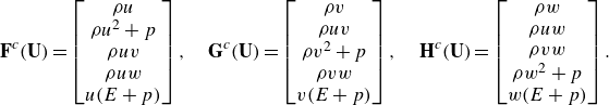 \begin{equation} \mathbf {F}^c(\mathbf {U}) = \begin{bmatrix} \rho u \\ \rho u^2 + p \\ \rho u v \\ \rho u w \\ u(E + p) \\ \end{bmatrix}, \quad \mathbf {G}^c(\mathbf {U}) = \begin{bmatrix} \rho v \\ \rho u v \\ \rho v^2 + p \\ \rho v w \\ v(E + p) \\ \end{bmatrix}, \quad \mathbf {H}^c(\mathbf {U}) = \begin{bmatrix} \rho w \\ \rho u w \\ \rho v w \\ \rho w^2 + p \\ w(E + p) \\ \end{bmatrix}. \end{equation}
The dissipative fluxes describe viscous effects and heat conduction:
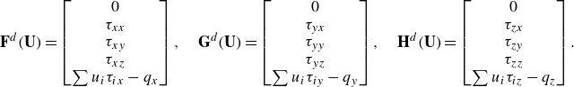 \begin{align} \mathbf {F}^d(\mathbf {U}) = \begin{bmatrix} 0 \\ \tau _{xx} \\ \tau _{xy} \\ \tau _{xz} \\ \sum u_i \tau _{ix} - q_x \\ \end{bmatrix}, \quad \mathbf {G}^d(\mathbf {U}) = \begin{bmatrix} 0 \\ \tau _{yx} \\ \tau _{yy} \\ \tau _{yz} \\ \sum u_i \tau _{iy} - q_y \\ \end{bmatrix}, \quad \mathbf {H}^d(\mathbf {U}) = \begin{bmatrix} 0 \\ \tau _{zx} \\ \tau _{zy} \\ \tau _{zz} \\ \sum u_i \tau _{iz} - q_z \\ \end{bmatrix}.\nonumber\\ \end{align}
The viscous stress is given by
 \begin{equation} \tau _{ij} = \mu \left ( \frac {\partial u_i}{\partial x_j} + \frac {\partial u_j}{\partial x_i} - \frac {2}{3}\delta _{ij}\frac {\partial u_k}{\partial x_k} \right ), \end{equation}
where $\mu$
is the dynamic viscosity. The energy flux vector
$\mu$
is the dynamic viscosity. The energy flux vector $\mathbf {q}= [q_x, q_y, q_z]^T$
is expressed via Fourier’s heat conduction law,
$\mathbf {q}= [q_x, q_y, q_z]^T$
is expressed via Fourier’s heat conduction law, $\mathbf {q} = -\lambda \nabla T$
, where
$\mathbf {q} = -\lambda \nabla T$
, where $\lambda$
is the heat conductivity.
$\lambda$
is the heat conductivity.
The system of governing equations is closed by the ideal gas equation of state:
 \begin{equation} p = (\gamma - 1)\rho e, \end{equation}
 \begin{equation} c = \sqrt {\frac {\gamma (p )}{\rho }}. \end{equation}
Here the ratio of specific heats $ \gamma = 1.4$
. In addition, we employ a simple power law model for the dynamic viscosity
$ \gamma = 1.4$
. In addition, we employ a simple power law model for the dynamic viscosity $ \mu$
,
$ \mu$
,
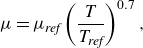 \begin{equation} \mu = \mu _{\textit{ref}} \left ( \frac {T}{T_{\textit{ref}}} \right )^{0.7}, \end{equation}
where $ \mu _{\textit{ref}}$
is the dynamic viscosity at the reference temperature
$ \mu _{\textit{ref}}$
is the dynamic viscosity at the reference temperature $ T_{\textit{ref}}$
. The thermal conductivity
$ T_{\textit{ref}}$
. The thermal conductivity $\lambda$
is determined using a constant Prandtl number
$\lambda$
is determined using a constant Prandtl number $Pr$
= 0.7:
$Pr$
= 0.7:
 \begin{equation} \lambda = \frac {Pr}{\unicode{x03BC} c_p}. \end{equation}
In this context, $ c_p$
represents the specific heat capacity at constant pressure.
$ c_p$
represents the specific heat capacity at constant pressure.
The source terms $ \mathbf {S(U)}$
in (2.1) represent body forces and heat sources. In the current study, a constant mass flow rate is maintained by applying a body force in the streamwise (
$ \mathbf {S(U)}$
in (2.1) represent body forces and heat sources. In the current study, a constant mass flow rate is maintained by applying a body force in the streamwise ( $x$
) direction using a proportional-integral-derivative (PID) controller that minimises the error between the target and current mass flow rate,
$x$
) direction using a proportional-integral-derivative (PID) controller that minimises the error between the target and current mass flow rate,
 \begin{equation} e(t) = \frac {\dot {m}_{ {target}} - \dot {m}(t)}{\dot {m}_{{target}}}. \end{equation}
The computational domain size ( $L_x/h \times L_y/h \times L_z/h$
) is
$L_x/h \times L_y/h \times L_z/h$
) is $ 3\pi \times 2 \times 1.5\pi$
in the streamwise (
$ 3\pi \times 2 \times 1.5\pi$
in the streamwise ( $x$
), wall-normal (
$x$
), wall-normal ( $y$
) and spanwise (
$y$
) and spanwise ( $z$
) directions, respectively (figure 1), where
$z$
) directions, respectively (figure 1), where $h$
is the channel half-width. The grid resolution consists of
$h$
is the channel half-width. The grid resolution consists of $ 192 \times 128 \times 96$
points in the corresponding
$ 192 \times 128 \times 96$
points in the corresponding $x \times y \times z$
directions. The DNS grid is uniform in the streamwise (
$x \times y \times z$
directions. The DNS grid is uniform in the streamwise ( $x$
) and spanwise (
$x$
) and spanwise ( $z$
) directions, while a hyperbolic-tangent stretching is applied in the wall-normal (
$z$
) directions, while a hyperbolic-tangent stretching is applied in the wall-normal ( $y$
) direction with a stretching factor of 1.8. The grid resolution in the streamwise and spanwise directions is
$y$
) direction with a stretching factor of 1.8. The grid resolution in the streamwise and spanwise directions is $\Delta x^+ = \Delta z^+ = 10.71$
, with
$\Delta x^+ = \Delta z^+ = 10.71$
, with $\Delta x^+=xu_\tau /\nu$
,
$\Delta x^+=xu_\tau /\nu$
, $\Delta z^+=zu_\tau /\nu$
and
$\Delta z^+=zu_\tau /\nu$
and $ u_\tau = \sqrt {\tau _w / \rho }$
. The cell sizes in the wall-normal direction vary, with a minimum value of
$ u_\tau = \sqrt {\tau _w / \rho }$
. The cell sizes in the wall-normal direction vary, with a minimum value of $\Delta y^+_{\textit{min}} = 0.69$
and a maximum value of
$\Delta y^+_{\textit{min}} = 0.69$
and a maximum value of $\Delta y^+_{ \textit{max}} = 6.48$
. A validation of the present DNS against the DNS data from Yao & Hussain (Reference Yao and Hussain2020) is provided in Appendix A.
$\Delta y^+_{ \textit{max}} = 6.48$
. A validation of the present DNS against the DNS data from Yao & Hussain (Reference Yao and Hussain2020) is provided in Appendix A.
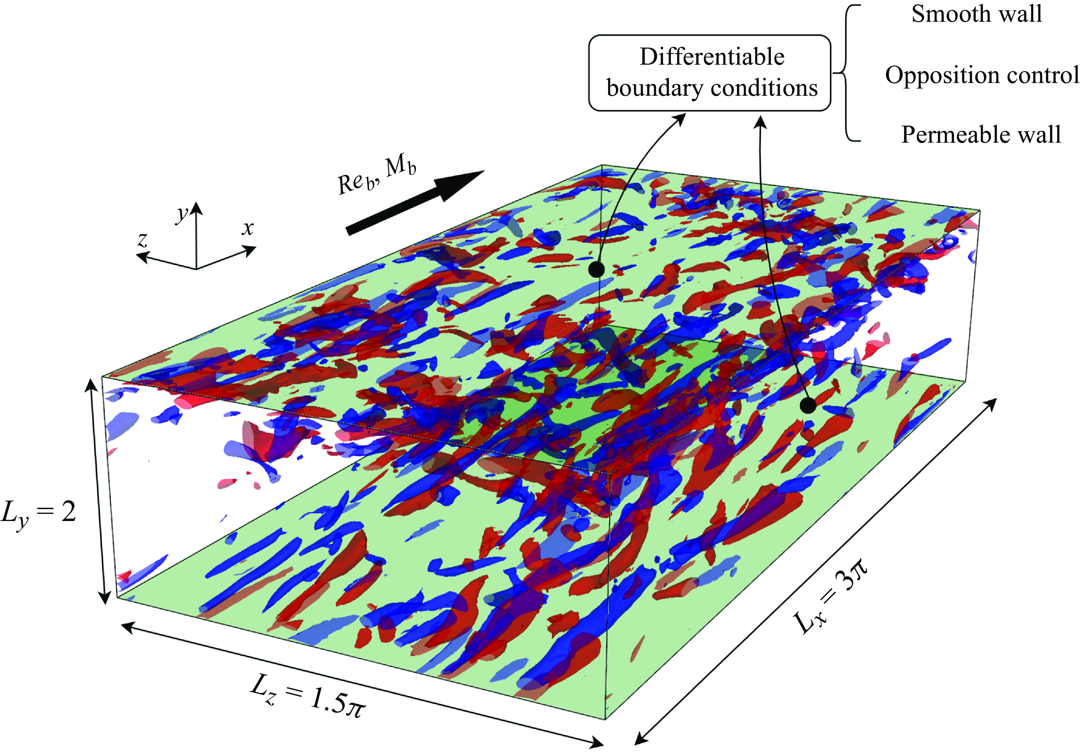
Figure 1. Domain of compressible DNS channel flow. The snapshot of the flow field, extracted from the smooth wall channel, serves as the initial condition for control. The blue and red isosurfaces represent streamwise vorticity at levels $\omega _x=\pm \sigma _x$
.
$\omega _x=\pm \sigma _x$
.
The bulk density is computed as $\rho _b = ({1}/{2h}) \int _{-h}^{h} \langle \rho \rangle \textrm {d}y$
and the bulk velocity is calculated as
$\rho _b = ({1}/{2h}) \int _{-h}^{h} \langle \rho \rangle \textrm {d}y$
and the bulk velocity is calculated as $ U_b = ({1}/{2h \rho _b}) \int _{-h}^{h} \langle \rho u \rangle \textrm {d}y$
. The Reynolds number, based on bulk density, bulk velocity, channel half-width and wall viscosity, is
$ U_b = ({1}/{2h \rho _b}) \int _{-h}^{h} \langle \rho u \rangle \textrm {d}y$
. The Reynolds number, based on bulk density, bulk velocity, channel half-width and wall viscosity, is $Re_b = ({\rho _b U_b h}/{\mu _w}) = 3000$
. The bulk Mach number, defined as the ratio of the bulk velocity to the speed of sound at the wall, is given by
$Re_b = ({\rho _b U_b h}/{\mu _w}) = 3000$
. The bulk Mach number, defined as the ratio of the bulk velocity to the speed of sound at the wall, is given by $ Ma_b = ({U_b}/{c_w}) = 1.5$
. Isothermal no-slip boundary conditions are enforced at the channel walls, where
$ Ma_b = ({U_b}/{c_w}) = 1.5$
. Isothermal no-slip boundary conditions are enforced at the channel walls, where $ T = 1$
and
$ T = 1$
and $ u = 0$
at
$ u = 0$
at $ y = \pm h$
. Periodic boundary conditions are applied in both the streamwise and spanwise directions.
$ y = \pm h$
. Periodic boundary conditions are applied in both the streamwise and spanwise directions.
For the numerical set-up, we employ a TENO6-A (Fu et al. Reference Fu, Hu and Adams2016) cell-face reconstruction method combined with a HLLC (Harten–Lax–van Leer contact) Riemann solver. The TENO6-A reconstruction is enhanced by an interpolation limiter, while flux limiters are not utilised in this work since the single-phase cases considered do not involve strong shock discontinuities. Diffusive fluxes are discretised using sixth-order central FD schemes, and the temporal evolution is carried out using a third-order TVD (total variation diminishing) Runge–Kutta (TVD-RK3) scheme with a Courant--Friedrichs--Lewy number of 0.9.
2.3. The flow control boundary conditions
In addition to the smooth wall channel flow, which is taken as the baseline of flow control performance, we investigate two types of flow control boundary conditions. The first is the boundary condition of opposition control. A wall-normal velocity
 \begin{equation} \boldsymbol {u}=-\phi (\boldsymbol {x},t)\cdot \boldsymbol {n} \end{equation}
is applied on the upper and lower wall, $\Gamma ^+$
and
$\Gamma ^+$
and $\Gamma ^-$
, where
$\Gamma ^-$
, where $\boldsymbol {n}$
is the unit outward normal to the boundary. This control strategy is applied with the objective of introducing a counteracting wall-normal velocity at the boundary, designed to oppose the near-wall turbulence structures. The total net flux across the boundary is constrained to be zero, i.e.
$\boldsymbol {n}$
is the unit outward normal to the boundary. This control strategy is applied with the objective of introducing a counteracting wall-normal velocity at the boundary, designed to oppose the near-wall turbulence structures. The total net flux across the boundary is constrained to be zero, i.e.
 \begin{equation} \int _{\Gamma ^+} \phi \textrm {d}\boldsymbol {x}=\int _{\Gamma ^-} \phi \textrm {d}\boldsymbol {x}=0, \end{equation}
ensuring that there is no net mass flow through the wall over time.
The second boundary condition is a permeable wall boundary condition proposed by Jiménez et al. (Reference Jiménez, Uhlmann, Pinelli and Kawahara2001). The wall-normal velocity on the lower and upper walls is modelled as
 \begin{equation} \boldsymbol {u} = -\beta (\boldsymbol {x},t) p'\cdot \boldsymbol {n}, \end{equation}
where the parameter $ \beta$
works like the permeability of the wall and modulates the coupling between the wall-normal velocity and the pressure fluctuations. The value of
$ \beta$
works like the permeability of the wall and modulates the coupling between the wall-normal velocity and the pressure fluctuations. The value of $ \beta$
varies in the range of 0--0.7, as suggested by Jiménez et al. (Reference Jiménez, Uhlmann, Pinelli and Kawahara2001). In contrast to the initial research of Jiménez et al. (Reference Jiménez, Uhlmann, Pinelli and Kawahara2001), where
$ \beta$
varies in the range of 0--0.7, as suggested by Jiménez et al. (Reference Jiménez, Uhlmann, Pinelli and Kawahara2001). In contrast to the initial research of Jiménez et al. (Reference Jiménez, Uhlmann, Pinelli and Kawahara2001), where $\beta$
remains constant throughout space and time, our approach considers
$\beta$
remains constant throughout space and time, our approach considers $\beta$
as variable in both dimensions in order to improve its control capabilities. For each time step,
$\beta$
as variable in both dimensions in order to improve its control capabilities. For each time step, $p'$
is computed by decomposition of
$p'$
is computed by decomposition of $p$
in the first layer of the grid above the wall
$p$
in the first layer of the grid above the wall $p=\langle p \rangle +p'$
. Here
$p=\langle p \rangle +p'$
. Here $\langle p \rangle$
is the average over the
$\langle p \rangle$
is the average over the $x$
--
$x$
-- $z$
plane, i.e.
$z$
plane, i.e. $\langle p \rangle =({1}/{L_xL_z})\int _\Gamma p \textrm {d}x \textrm {d} z$
;
$\langle p \rangle =({1}/{L_xL_z})\int _\Gamma p \textrm {d}x \textrm {d} z$
; $p'$
is the current step used to compute the wall velocity for the next step. This ensures that
$p'$
is the current step used to compute the wall velocity for the next step. This ensures that $\langle p' \rangle =0$
, and therefore, there is no net flux across the wall when
$\langle p' \rangle =0$
, and therefore, there is no net flux across the wall when $\beta$
has a uniform spatial distribution. The net flux across the wall is only attributed to the spatial variation of
$\beta$
has a uniform spatial distribution. The net flux across the wall is only attributed to the spatial variation of $\beta$
.
$\beta$
.
Note that the isothermal condition ( $T=1$
) is applied to the channel walls for both the opposition control and permeable wall boundary conditions. This is consistent with the baseline case of smooth wall channel.
$T=1$
) is applied to the channel walls for both the opposition control and permeable wall boundary conditions. This is consistent with the baseline case of smooth wall channel.
2.4. Optimisation workflow
Figure 2 illustrates the workflow for the AD-based optimisation. We adopted the receding-horizon predictive control process introduced by Bewley et al. (Reference Bewley, Moin and Temam2001). The evolution of the flow consists of a series of ‘episodes’. In each episode, the optimised control parameters are explored by an iterative gradient-based optimisation algorithm. Once this iteration converges, the flow is advanced to the next episode and the optimisation process is initiated again.
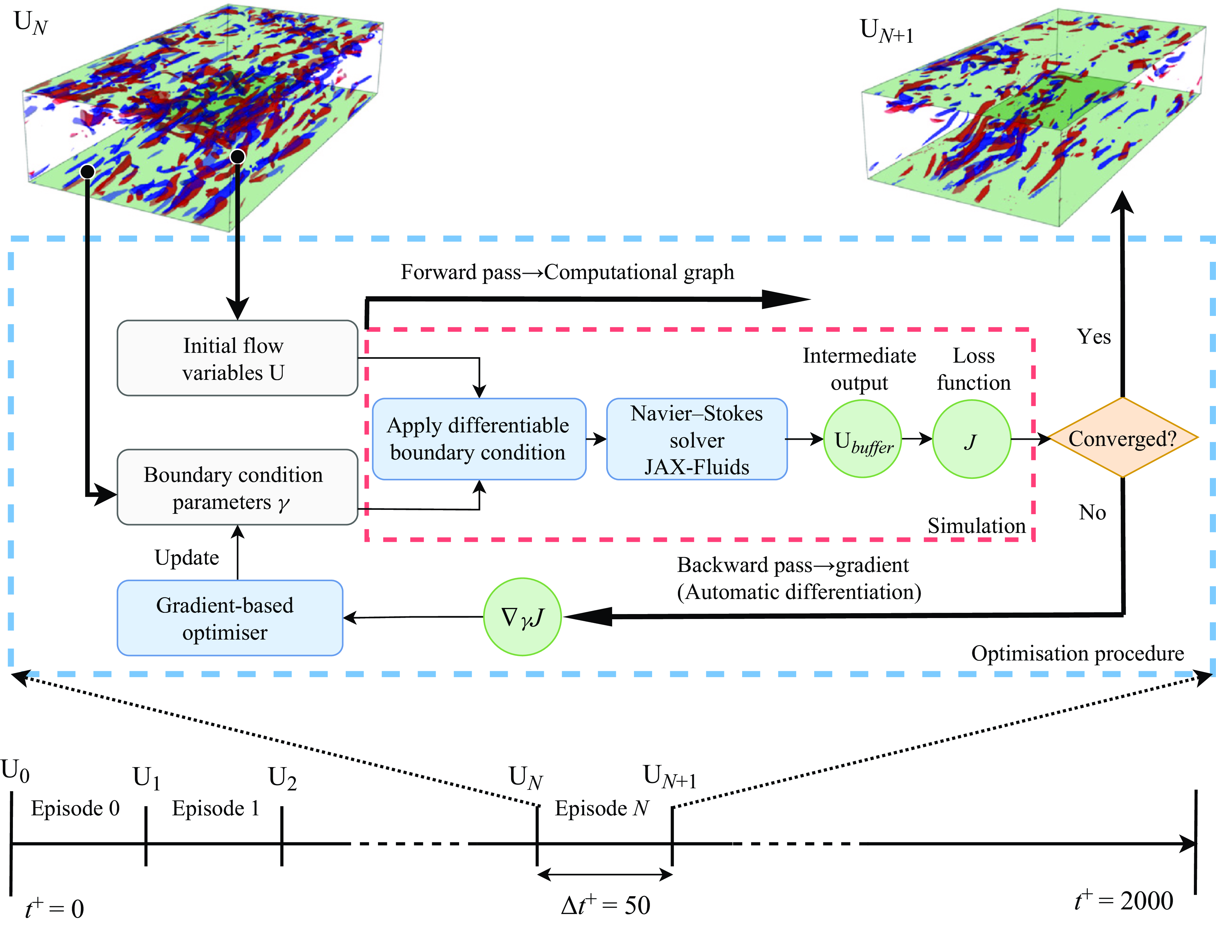
Figure 2. The procedure for AD and flow control optimisation.
Consider episode $N$
as an instance. The optimisation’s input is
$N$
as an instance. The optimisation’s input is $\textbf {U}_N$
, representing the terminal state from episode
$\textbf {U}_N$
, representing the terminal state from episode $N-1$
. Alongside the boundary condition parameters for the upper and lower walls,
$N-1$
. Alongside the boundary condition parameters for the upper and lower walls, $\gamma$
, the initial flow variables are processed through the differentiable solver to yield an intermediate output
$\gamma$
, the initial flow variables are processed through the differentiable solver to yield an intermediate output $\textbf {U}_{ \textit{buffer}}$
, which is used to calculate the loss function
$\textbf {U}_{ \textit{buffer}}$
, which is used to calculate the loss function $J$
. During the forward computation, the computational graph is created, allowing for the calculation of the gradient of the loss function concerning the boundary parameter
$J$
. During the forward computation, the computational graph is created, allowing for the calculation of the gradient of the loss function concerning the boundary parameter $\nabla _{\gamma } J(\gamma )$
via AD. This requires just one computation pass to form the graph.
$\nabla _{\gamma } J(\gamma )$
via AD. This requires just one computation pass to form the graph.
The gradient-based optimiser then updates the control input for differentiable boundary conditions. In this context, the Adam optimiser (Kingma Reference Kingma2014) is used. At each iteration $k$
, the gradients
$k$
, the gradients $\nabla _{\gamma } J(\gamma )$
are used to calculate the biased first moment
$\nabla _{\gamma } J(\gamma )$
are used to calculate the biased first moment $m_k$
and the biased second moment
$m_k$
and the biased second moment $v_k$
of the gradients according to the update rules
$v_k$
of the gradients according to the update rules
 \begin{equation} m_k = \beta _1 m_{k-1} + (1 - \beta _1) \nabla _{\gamma } J(\gamma ), \end{equation}
 \begin{equation} v_k = \beta _2 v_{k-1} + (1 - \beta _2) (\nabla _{\gamma } J(\gamma ))^2, \end{equation}
where $\beta _1$
and
$\beta _1$
and $\beta _2$
are the exponential decay rates for the first and second moments. Here we use
$\beta _2$
are the exponential decay rates for the first and second moments. Here we use $\beta _1=0.9$
and
$\beta _1=0.9$
and $\beta _2=0.999$
. To correct the biases introduced by initialising the moments to zero, the bias-corrected first and second moments are computed as
$\beta _2=0.999$
. To correct the biases introduced by initialising the moments to zero, the bias-corrected first and second moments are computed as
 \begin{equation} \hat {m}_k = \frac {m_k}{1 - \beta _1^k}, \quad \hat {v}_k = \frac {v_k}{1 - \beta _2^k}. \end{equation}
Finally, the control parameters are updated using these corrected moments, i.e.
 \begin{equation} \gamma _{k+1} = \gamma _k - \alpha \frac {\hat {m}_k}{\sqrt {\hat {v}_k} + \epsilon }, \end{equation}
where $\alpha$
is the learning rate and
$\alpha$
is the learning rate and $\epsilon =10^{-7}$
is a small constant to avoid dividing by zero. In the current study the learning rate
$\epsilon =10^{-7}$
is a small constant to avoid dividing by zero. In the current study the learning rate $\alpha$
is set to 0.01. The iteration process continues until the relative magnitude of the loss function reduction becomes sufficiently small, ensuring convergence:
$\alpha$
is set to 0.01. The iteration process continues until the relative magnitude of the loss function reduction becomes sufficiently small, ensuring convergence:
 \begin{equation} \frac {|J(\gamma _{k+1}) - J(\gamma _k)|}{|J(\gamma _k)|} \lt \delta . \end{equation}
Here $\delta$
is
$\delta$
is $10^{-4}$
. For each episode, the maximum iteration limit is set to 100 steps to balance computational efficiency and optimisation accuracy. When optimisation converges, the boundary condition parameters are fixed for the current episode, enabling the flow to proceed by
$10^{-4}$
. For each episode, the maximum iteration limit is set to 100 steps to balance computational efficiency and optimisation accuracy. When optimisation converges, the boundary condition parameters are fixed for the current episode, enabling the flow to proceed by $\Delta t$
and generate the terminal flow state
$\Delta t$
and generate the terminal flow state $\textbf {U}_{N+1}$
. While the Adam method used in this study is suited for managing sparse gradients, it might reach suboptimal solutions in some non-convex optimisation problems. Hence, it is important to carefully examine the convergence of optimisation. Further analysis of the performance of the Adam optimiser will be provided in later sections.
$\textbf {U}_{N+1}$
. While the Adam method used in this study is suited for managing sparse gradients, it might reach suboptimal solutions in some non-convex optimisation problems. Hence, it is important to carefully examine the convergence of optimisation. Further analysis of the performance of the Adam optimiser will be provided in later sections.
For the current channel domain, the upper and lower walls consist of $192\times 96\times 2$
grid points, resulting in a
$192\times 96\times 2$
grid points, resulting in a $36\,864$
dimensional optimisation problem. Automatic differentiation is particularly powerful with functions with such high-dimensional input. Only one backward pass through the computational graph is needed to compute the gradient with respect to all input variables, since each partial derivative is accumulated in parallel during the backward pass. Therefore, the total cost remains low even as the input dimension increases. In addition, JAX uses the XLA (accelerated linear algebra) compiler for just-in-time (JIT) compilation of functions. The JIT compilation translates the Python functions into a lower-level, optimised representation that can run directly on the hardware, avoiding the overhead of Python’s interpreter. This is particularly beneficial for AD, where operations need to be traced through a computational graph. With JIT, this tracing happens once and the compiled version can be executed repeatedly without needing to retrace.
$36\,864$
dimensional optimisation problem. Automatic differentiation is particularly powerful with functions with such high-dimensional input. Only one backward pass through the computational graph is needed to compute the gradient with respect to all input variables, since each partial derivative is accumulated in parallel during the backward pass. Therefore, the total cost remains low even as the input dimension increases. In addition, JAX uses the XLA (accelerated linear algebra) compiler for just-in-time (JIT) compilation of functions. The JIT compilation translates the Python functions into a lower-level, optimised representation that can run directly on the hardware, avoiding the overhead of Python’s interpreter. This is particularly beneficial for AD, where operations need to be traced through a computational graph. With JIT, this tracing happens once and the compiled version can be executed repeatedly without needing to retrace.
The duration of the optimisation episodes plays a vital role in the system. This time horizon influences how far ahead the control algorithm projects the system’s behaviour. A longer horizon enables the controller to foresee long-term effects of its actions, though it demands more computational power. Conversely, a shorter horizon decreases computational effort and favours real-time execution, but might lead to less optimal decisions. In our current study we evaluated two time horizons: $\Delta t^+=\Delta t u^2_\tau /\nu _w=25$
and
$\Delta t^+=\Delta t u^2_\tau /\nu _w=25$
and $50$
, with the latter corresponding to a 0.69 flow-through time
$50$
, with the latter corresponding to a 0.69 flow-through time $tU_b/L_x$
. The rollout time step is
$tU_b/L_x$
. The rollout time step is $\Delta t_{\textit{rollout}}^+=0.04$
, which results in 1250 rollout steps for an episode with a time horizon of
$\Delta t_{\textit{rollout}}^+=0.04$
, which results in 1250 rollout steps for an episode with a time horizon of $\Delta t^+=50$
. In comparison, Bewley et al. (Reference Bewley, Moin and Temam2001) used
$\Delta t^+=50$
. In comparison, Bewley et al. (Reference Bewley, Moin and Temam2001) used $\Delta t_{\textit{rollout}}^+=0.14$
for control optimisation with the adjoint method in an incompressible turbulent channel at
$\Delta t_{\textit{rollout}}^+=0.14$
for control optimisation with the adjoint method in an incompressible turbulent channel at $Re_\tau =180$
. Meanwhile, Sonoda et al. (Reference Sonoda, Liu, Itoh and Hasegawa2023) used RL to optimise opposition control, using
$Re_\tau =180$
. Meanwhile, Sonoda et al. (Reference Sonoda, Liu, Itoh and Hasegawa2023) used RL to optimise opposition control, using $\Delta t_{\textit{rollout}}^+=0.06$
for the minimal channel and
$\Delta t_{\textit{rollout}}^+=0.06$
for the minimal channel and $\Delta t_{\textit{rollout}}^+=0.03$
for a full-size channel at
$\Delta t_{\textit{rollout}}^+=0.03$
for a full-size channel at $Re_\tau =150$
. We tested that the optimisation results are only weakly dependent on the choice of
$Re_\tau =150$
. We tested that the optimisation results are only weakly dependent on the choice of $\Delta t_{\textit{rollout}}$
. The total simulation runs for
$\Delta t_{\textit{rollout}}$
. The total simulation runs for $ t^+ = 2000$
, translating to 27.6 flow-through times, which is adequate for the controlling boundary to significantly affect turbulent flow dynamics. The simulation and optimisation processes utilise eight NVIDIA A100 GPUs on a single node within the HAWK-AI infrastructure at the High Performance Computing Center Stuttgart. Each optimisation with
$ t^+ = 2000$
, translating to 27.6 flow-through times, which is adequate for the controlling boundary to significantly affect turbulent flow dynamics. The simulation and optimisation processes utilise eight NVIDIA A100 GPUs on a single node within the HAWK-AI infrastructure at the High Performance Computing Center Stuttgart. Each optimisation with $ t^+ = 2000$
takes about two days of wall-clock time. This duration is manageable for industrial applications, highlighting its potential in practical optimisation tasks.
$ t^+ = 2000$
takes about two days of wall-clock time. This duration is manageable for industrial applications, highlighting its potential in practical optimisation tasks.
Note that we use single precision in all simulations. This decision balances computational efficiency with accuracy. Automatic differentiation computations require substantial memory and time, and we verified that turbulence statistics in current low-Reynolds-number channel flow simulations using single precision closely match those with double precision, as validated in Appendix A. Thus, we selected single precision on GPUs for our tests. This offers us greater flexibility in computational domain size and time horizon, which we prioritise over slightly diminished precision.
2.5. Loss functions
The choice of loss function has a large impact on the optimisation process. In the current study we compare several types of loss functions.
2.5.1. Cumulative wall friction control
To consider the cumulative effect of wall friction $\tau _w=\mu ( {\partial u}/{\partial y} )_{y=0}$
, the loss function can be formulated as the integration of friction drag on the upper and lower walls and over the time horizon (0,
$\tau _w=\mu ( {\partial u}/{\partial y} )_{y=0}$
, the loss function can be formulated as the integration of friction drag on the upper and lower walls and over the time horizon (0, $\Delta t$
). For the opposition control strategy, the magnitude of
$\Delta t$
). For the opposition control strategy, the magnitude of $\phi$
also needs to be constrained to limit the cost of control, i.e.
$\phi$
also needs to be constrained to limit the cost of control, i.e.
 \begin{equation} J_{\tau (\textit{cum})}(\phi )=-\frac {1}{\Delta t}\int _0^{\Delta t} \int _{\Gamma ^{ \pm }} \mu \frac {\partial u(\phi )}{\partial n} \textrm {d} \boldsymbol {x} \textrm {d} t+\frac {\ell ^2}{2} \int _{\Gamma ^{ \pm }}\rho _w \phi ^2 \textrm {d} \boldsymbol {x} , \end{equation}
where $\partial / \partial n$
represents the gradient in the direction perpendicular to the wall, facing outward. The factor
$\partial / \partial n$
represents the gradient in the direction perpendicular to the wall, facing outward. The factor $\ell ^2$
represents the price of control, which regulates the importance of the control cost in the loss function, and hence, affects the optimisation result of
$\ell ^2$
represents the price of control, which regulates the importance of the control cost in the loss function, and hence, affects the optimisation result of $\phi$
. In the current work we choose
$\phi$
. In the current work we choose $\ell ^2$
to be 1. As will be shown later, this is a relatively large constraint on the input energy of opposition control and results in a small amplitude of
$\ell ^2$
to be 1. As will be shown later, this is a relatively large constraint on the input energy of opposition control and results in a small amplitude of $\phi$
.
$\phi$
.
For permeable wall cases, there is no energy consumption except at the state-changing instants between control sections. In this study we ideally assume that the state-changing process of permeable walls has a marginal cost; hence, the cost function for permeable wall cases is
 \begin{equation} J_{\tau (\textit{cum})}(\beta )=-\frac {1}{\Delta t}\int _0^{\Delta t} \int _{\Gamma ^{ \pm }} \mu \frac {\partial u(\beta )}{\partial n} \textrm {d} \boldsymbol {x} \textrm {d} t. \end{equation}
2.5.2. Cumulative turbulent kinetic energy control
In the present study, the longest time horizon for each episode, $\Delta t^+ = 50$
, corresponds to 0.69 of the flow-through time. This is similar to the time horizon employed in earlier research (Bewley et al. Reference Bewley, Moin and Temam2001), yet it remains insufficient for the entire channel to fully stabilise following the implementation of control. Therefore, taking the quantity of interest directly as the cost function may not be the most effective and stable means of reducing it over the long term. In particular, wall friction only involves the information on the wall, which can be manipulated easily by setting the boundary condition in a short period. The potential long-term effects of these manipulations on the outer region are not taken into account, which may lead to instability of the control results.
$\Delta t^+ = 50$
, corresponds to 0.69 of the flow-through time. This is similar to the time horizon employed in earlier research (Bewley et al. Reference Bewley, Moin and Temam2001), yet it remains insufficient for the entire channel to fully stabilise following the implementation of control. Therefore, taking the quantity of interest directly as the cost function may not be the most effective and stable means of reducing it over the long term. In particular, wall friction only involves the information on the wall, which can be manipulated easily by setting the boundary condition in a short period. The potential long-term effects of these manipulations on the outer region are not taken into account, which may lead to instability of the control results.
Turbulence in the near-wall region induces wall-normal convective transport, thereby enhancing both drag and heat transfer in the flow. It is well known that turbulent production throughout the channel significantly contributes to wall friction (Renard & Deck Reference Renard and Deck2016). Hence, alleviating turbulence intensity might lead to a reduction in wall friction. Moreover, turbulent kinetic energy (TKE), in contrast to wall friction that is concentrated in the region close to the wall, results from the turbulence sustaining processes occurring throughout the entire channel. Consequently, TKE may serve as a more effective loss function than wall friction in producing stable control outcomes. We employed the cumulative TKE across the channel as the loss function. For the opposition control boundary, we also include the constraint on the cost of control:
 \begin{equation} J_{k(\textit{cum})}(\phi )=\frac {1}{4h\Delta t} \int _0^{\Delta t} \int _{\Omega } \rho |\boldsymbol {u}(\phi )|^2 \textrm {d} \boldsymbol {x} \textrm {d} t+\frac {\ell ^2}{2} \int _{\Gamma ^{ \pm }}\rho _w \phi ^2 \textrm {d} \boldsymbol {x}. \end{equation}
For the permeable wall case, The cost of control is assumed to be small and not taken into consideration hence the loss function is
 \begin{equation} J_{k(\textit{cum})}(\beta )=\frac {1}{4h\Delta t} \int _0^{\Delta t} \int _{\Omega } \rho |\boldsymbol {u}(\beta )|^2 \textrm {d} \boldsymbol {x} \textrm {d} t. \end{equation}
2.5.3. Terminal wall friction and TKE control
In addition to cumulative control that considers wall friction or TKE throughout the time horizon, another control method is to concentrate solely on the terminal value of each episode. Using the terminal control approach, the cost functional does not penalise deviations in the quantity of interest during the intermediate stages of each episode, provided that these deviations result in lower values of the quantity of interest at the end of each optimisation horizon. Compared with traditional methods, the terminal control approach offers greater flexibility in control strategies and potentially better control outcomes; however, choosing an inappropriate loss function and having a very short time horizon may also result in instability.
For terminal wall friction minimisation with opposition control, the loss function is
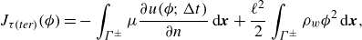 \begin{equation} J_{\tau (\textit{ter})}(\phi )=-\int _{\Gamma ^{ \pm }} \mu \frac {\partial u(\phi ;\Delta t)}{\partial n} \textrm {d} \boldsymbol {x}+\frac {\ell ^2}{2} \int _{\Gamma ^{ \pm }}\rho _w \phi ^2 \textrm {d} \boldsymbol {x}, \end{equation}
and the loss function for a permeable wall is
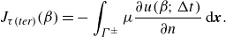 \begin{equation} J_{\tau (\textit{ter})}(\beta )=-\int _{\Gamma ^{ \pm }} \mu \frac {\partial u(\beta ;\Delta t)}{\partial n} \textrm {d} \boldsymbol {x}. \end{equation}
Similarly, the loss functions for terminal TKE minimisation are
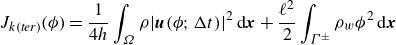 \begin{equation} J_{k(\textit{ter})}(\phi )=\frac {1}{4h} \int _{\Omega } \rho |\boldsymbol {u}(\phi ;\Delta t)|^2 \textrm {d} \boldsymbol {x}+\frac {\ell ^2}{2} \int _{\Gamma ^{ \pm }}\rho _w \phi ^2 \textrm {d} \boldsymbol {x} \end{equation}
and
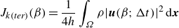 \begin{equation} J_{k(\textit{ter})}(\beta )=\frac {1}{4h} \int _{\Omega } \rho |\boldsymbol {u}(\beta ;\Delta t)|^2 \textrm {d} \boldsymbol {x} \end{equation}
for opposition control and a permeable wall, respectively.
3. Results
In the current section we show the simulation with optimised opposition control and permeable wall configurations.
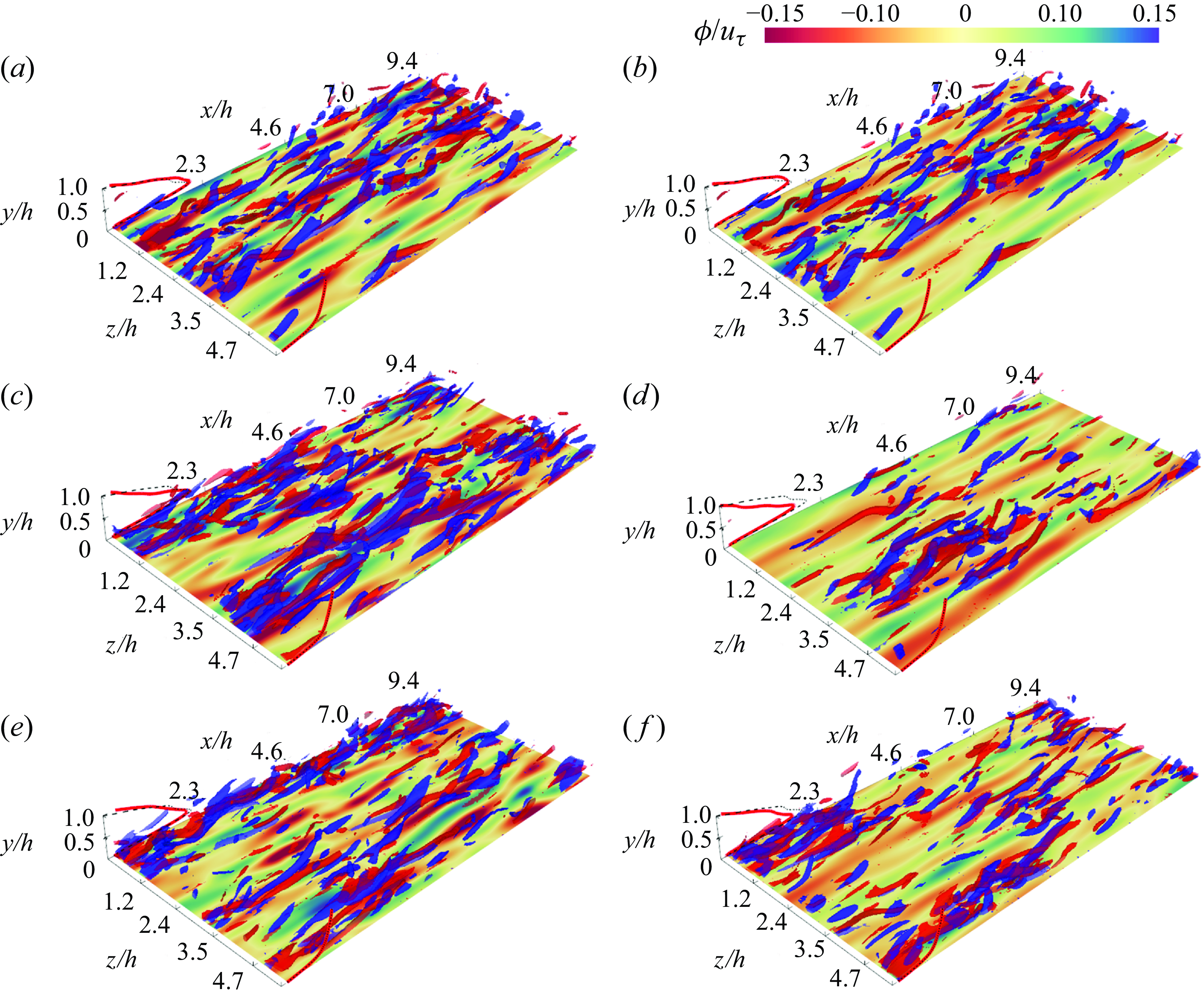
Figure 3. Vorticity structures above opposition control surfaces. Panels (a,c,e) show cumulative wall friction control with $\Delta t^+=50$
, while panels (b,d,f) depict terminal TKE control with the same
$\Delta t^+=50$
, while panels (b,d,f) depict terminal TKE control with the same $\Delta t^+$
. The pairs of panels (a,b), (c,d) and (e,f) represent
$\Delta t^+$
. The pairs of panels (a,b), (c,d) and (e,f) represent $t^+=50$
,
$t^+=50$
, $t^+=500$
and
$t^+=500$
and $t^+=2000$
from the onset of control, respectively. Blue and red isosurfaces indicate streamwise vorticity at
$t^+=2000$
from the onset of control, respectively. Blue and red isosurfaces indicate streamwise vorticity at $\omega _x=\pm \sigma _{\omega _x}$
,
$\omega _x=\pm \sigma _{\omega _x}$
, $\sigma _{\omega _x}$
being the standard deviation of
$\sigma _{\omega _x}$
being the standard deviation of $\omega _x$
at
$\omega _x$
at $t=0$
. Control
$t=0$
. Control $\phi$
is illustrated on the wall with coloured contours. Present snapshot profiles of
$\phi$
is illustrated on the wall with coloured contours. Present snapshot profiles of $\langle u\rangle$
and
$\langle u\rangle$
and $-\langle u'v'\rangle$
are overlaid on front (
$-\langle u'v'\rangle$
are overlaid on front ( $z=1.5\pi$
) and back (
$z=1.5\pi$
) and back ( $z=0$
) planes with solid red lines. Black dashed lines show profiles from the smooth wall scenario for comparison. See also supplementary movies 1 and 2 for the full simulation duration.
$z=0$
) planes with solid red lines. Black dashed lines show profiles from the smooth wall scenario for comparison. See also supplementary movies 1 and 2 for the full simulation duration.
3.1. The performance of opposition control
The performance of opposition control is determined by the control $\phi (t)$
, which is influenced by the configuration of the optimisation process. Since we use the auto-differentiation gradient as the optimisation input, the form of the computational graph is the core. For the current set-up, there are two important factors. First, the time horizon of the episodes decides the time integration length of the Navier–Stokes equation, and hence, is closely related to the complexity of the computational graph. It also defines the maximum flow field information available from the temporal dimension that could be utilised for optimisation. Physically, the time horizon is the period during which the flow is allowed to develop under the same conditions
$\phi (t)$
, which is influenced by the configuration of the optimisation process. Since we use the auto-differentiation gradient as the optimisation input, the form of the computational graph is the core. For the current set-up, there are two important factors. First, the time horizon of the episodes decides the time integration length of the Navier–Stokes equation, and hence, is closely related to the complexity of the computational graph. It also defines the maximum flow field information available from the temporal dimension that could be utilised for optimisation. Physically, the time horizon is the period during which the flow is allowed to develop under the same conditions $\phi$
. Second, the choice of loss function also profoundly affects the computational graph, since it determines more specifically the variables, as well as the spatial and temporal range, included in the computational graph. Figure 3 shows the comparison of instantaneous flow fields with different optimisation targets.
$\phi$
. Second, the choice of loss function also profoundly affects the computational graph, since it determines more specifically the variables, as well as the spatial and temporal range, included in the computational graph. Figure 3 shows the comparison of instantaneous flow fields with different optimisation targets.
Initially, the vortices exhibit a similar shape and count in both scenarios at the early stage of control ( $t^+=50$
). However, as the flow continues to evolve (
$t^+=50$
). However, as the flow continues to evolve ( $t^+=500$
and 2000), the vortex structures diverge markedly in form and quantity between the two cases. In the cumulative wall friction control scenario (figure 3
a,c,e), the vortices become more intense, whereas in the TKE control scenario (figure 3
b,d,f), the turbulent structures are notably diminished. This divergence is evident in the mean statistics, such as the Reynolds stress profile
$t^+=500$
and 2000), the vortex structures diverge markedly in form and quantity between the two cases. In the cumulative wall friction control scenario (figure 3
a,c,e), the vortices become more intense, whereas in the TKE control scenario (figure 3
b,d,f), the turbulent structures are notably diminished. This divergence is evident in the mean statistics, such as the Reynolds stress profile $\langle u'v'\rangle$
(indicated by red solid lines on the plane
$\langle u'v'\rangle$
(indicated by red solid lines on the plane $z=0$
). Compared with the initial
$z=0$
). Compared with the initial $\langle u'v'\rangle$
(denoted by black dashed lines on the plane
$\langle u'v'\rangle$
(denoted by black dashed lines on the plane $z=0$
), the wall friction control case shows a slight increase in the magnitude of Reynolds stress, while the TKE control case registers a significant reduction in the peak of Reynolds stress.
$z=0$
), the wall friction control case shows a slight increase in the magnitude of Reynolds stress, while the TKE control case registers a significant reduction in the peak of Reynolds stress.
The rise in Reynolds stress in the case of wall friction control appears counterintuitive as Reynolds stress significantly contributes to friction drag. This is due to the modification of the mean velocity profile $\langle u\rangle$
by the control. However, this alteration is localised near the wall and is not distinctly visible (the
$\langle u\rangle$
by the control. However, this alteration is localised near the wall and is not distinctly visible (the $\langle u\rangle$
profiles are depicted as red solid lines in the plane
$\langle u\rangle$
profiles are depicted as red solid lines in the plane $z=1.5\pi$
in figure 3).
$z=1.5\pi$
in figure 3).
It is also worth noting that $\phi$
remains constant in each episode. This means that
$\phi$
remains constant in each episode. This means that $\phi$
updates at a low frequency, making it more advantageous for practical implementation. However, since each episode’s optimisation is independent, there could be
$\phi$
updates at a low frequency, making it more advantageous for practical implementation. However, since each episode’s optimisation is independent, there could be $\phi$
discontinuities between consecutive episodes (see supplementary movies 1 and 2 available at https://doi.org/10.1017/jfm.2025.304). This could be problematic for real-world flow control, as actuator response times may not handle sudden
$\phi$
discontinuities between consecutive episodes (see supplementary movies 1 and 2 available at https://doi.org/10.1017/jfm.2025.304). This could be problematic for real-world flow control, as actuator response times may not handle sudden $\phi$
changes, potentially affecting control performance. Such a gap between the ideal
$\phi$
changes, potentially affecting control performance. Such a gap between the ideal $\phi$
and real control velocity can be narrowed by using more efficient actuators with a shorter reaction time. Another way to improve the continuity of
$\phi$
and real control velocity can be narrowed by using more efficient actuators with a shorter reaction time. Another way to improve the continuity of $\phi$
is to use a time-varying control field per episode. This could potentially reduce the temporal discontinuities of
$\phi$
is to use a time-varying control field per episode. This could potentially reduce the temporal discontinuities of $\phi$
, but the extra temporal dimension of the control parameter would greatly increase the computational demands. In this study we overlook how this
$\phi$
, but the extra temporal dimension of the control parameter would greatly increase the computational demands. In this study we overlook how this $\phi$
discontinuity might affect real-world applications and assume that the ‘actuators’ function perfectly.
$\phi$
discontinuity might affect real-world applications and assume that the ‘actuators’ function perfectly.
In the following sections we assess the impact of control strategies across varying time horizons and loss functions. We elucidate the drag reduction mechanisms for different scenarios in more detail.
3.1.1. The development of wall friction under opposition control
In § 2.5 we introduced two types of loss functions directly targeting wall friction: the first, $J_{\tau (\textit{cum})}$
, takes into account wall friction over the entire time horizon, while the second,
$J_{\tau (\textit{cum})}$
, takes into account wall friction over the entire time horizon, while the second, $J_{\tau (\textit{ter})}$
, focuses solely on the terminal value for each episode. Figure 4 presents a comparison of the drag evolution history using both types of loss functions, analysed over two different time horizon durations,
$J_{\tau (\textit{ter})}$
, focuses solely on the terminal value for each episode. Figure 4 presents a comparison of the drag evolution history using both types of loss functions, analysed over two different time horizon durations, $\Delta t^+=25$
and
$\Delta t^+=25$
and $50$
.
$50$
.
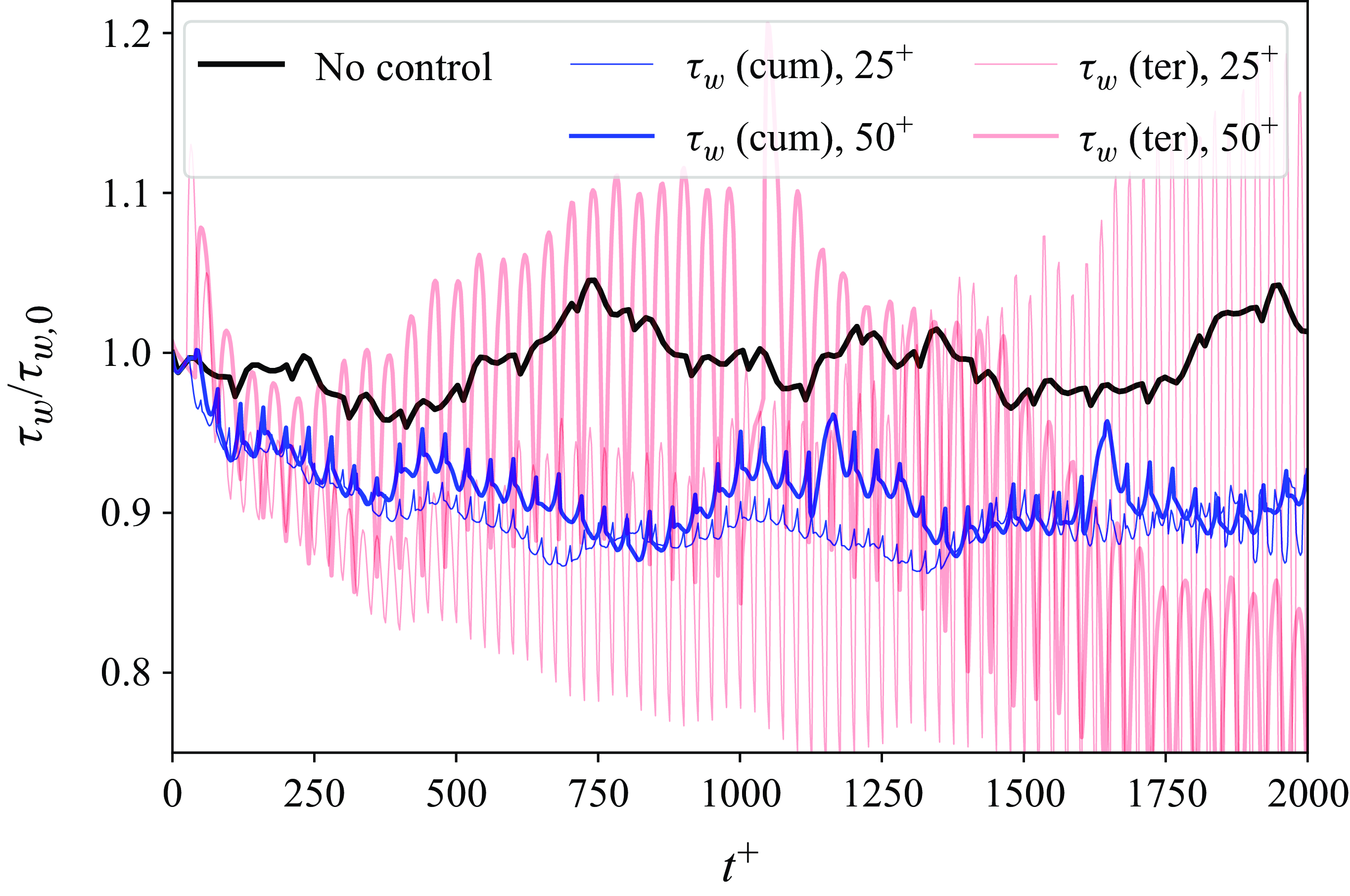
Figure 4. The development of wall friction $\tau _w$
with opposition control directly targeting loss functions associated with
$\tau _w$
with opposition control directly targeting loss functions associated with $\tau _w$
. In the legend, ‘
$\tau _w$
. In the legend, ‘ $\tau _w$
(cum),
$\tau _w$
(cum), $25^+$
’ represents cumulative wall friction control with a time horizon of
$25^+$
’ represents cumulative wall friction control with a time horizon of $\Delta t^+=25$
; ‘
$\Delta t^+=25$
; ‘ $\tau _w$
(ter)’ indicates terminal wall friction control. This convention is consistently applied throughout the rest of the legend and the paper.
$\tau _w$
(ter)’ indicates terminal wall friction control. This convention is consistently applied throughout the rest of the legend and the paper.
For the cumulative $\tau _w$
control, the wall friction reduces to approximately 90 % of its initial value by
$\tau _w$
control, the wall friction reduces to approximately 90 % of its initial value by $t^+=750$
. A slight improvement in control outcomes is observed with a shorter time horizon of
$t^+=750$
. A slight improvement in control outcomes is observed with a shorter time horizon of $\Delta t^+=25$
. In contrast, when employing a terminal loss function
$\Delta t^+=25$
. In contrast, when employing a terminal loss function $J_{\tau (\textit{ter})}$
and a time horizon of
$J_{\tau (\textit{ter})}$
and a time horizon of $\Delta t^+=25$
, wall friction decreases by approximately 13 % at
$\Delta t^+=25$
, wall friction decreases by approximately 13 % at $t^+=400$
, which seems to be more effective than cumulative control. However, after
$t^+=400$
, which seems to be more effective than cumulative control. However, after $t^+=500$
, the performance deteriorates, exhibiting a significant fluctuation as well as a slow recovery in wall friction. This issue is exacerbated when terminal control is paired with an extended time horizon
$t^+=500$
, the performance deteriorates, exhibiting a significant fluctuation as well as a slow recovery in wall friction. This issue is exacerbated when terminal control is paired with an extended time horizon $\Delta t^+=50$
, as the wall friction experiences strong fluctuations and fails to stabilise within the tested interval.
$\Delta t^+=50$
, as the wall friction experiences strong fluctuations and fails to stabilise within the tested interval.
The unstable performance of terminal control aligns with our expectations. As described in § 2.5, focusing solely on the terminal value can lead to situations where only terminal friction is decreased. This is particularly true when combined with a wall friction-based loss function, as only the data points right above the wall are incorporated into the computational graph. In such cases, much of the channel flow dynamics is curtailed, and this truncation increases with longer time horizons. By focusing on the near-wall region and neglecting the rest of the turbulent channel, terminal control can become more aggressive and effective in the short term. However, this short-sighted approach may cause excessive disturbances, ultimately increasing turbulent fluctuations over time. To counteract the rise in wall friction from additional turbulence, terminal control requires more intense intervention, creating a vicious cycle and resulting in control instability. The cumulative loss function, which considers the full evolution history of wall friction, offers an advantage by implicitly involving the dynamics of the outer region in the computational graph. Consequently, while cumulative control may take longer to demonstrate its effects, it tends to be more stable.
An alternative method to reduce wall friction involves suppressing the turbulence intensity within the channel, which is also the fundamental principle behind opposition control (Choi et al. Reference Choi, Moin and Kim1994). We also compare the performance of the cumulative and terminal type of loss function, i.e. $J_{k{(\textit{cum})}}$
and
$J_{k{(\textit{cum})}}$
and $J_{k{(\textit{ter})}}$
, under time horizons
$J_{k{(\textit{ter})}}$
, under time horizons $\Delta t^+=25$
and
$\Delta t^+=25$
and $\Delta t^+=50$
.
$\Delta t^+=50$
.
Figure 5(a) depicts the TKE evolution following the implementation of opposition control. With cumulative controls, TKE decreases by around 20 % at $t^+=250$
. Initially, TKE declines slightly quicker with an extended time horizon, yet the difference between
$t^+=250$
. Initially, TKE declines slightly quicker with an extended time horizon, yet the difference between $\Delta t^+=25$
and 50 becomes insignificant after
$\Delta t^+=25$
and 50 becomes insignificant after $t^+=750$
. Terminal controls seem more efficient, lowering TKE by approximately 34 % at
$t^+=750$
. Terminal controls seem more efficient, lowering TKE by approximately 34 % at $t^+=250$
. An extended time horizon seems advantageous for enhancing control performance. Despite a gradual recovery after the initial quick drop, the turbulence intensity remains significantly lower compared with the cumulative control scenarios.
$t^+=250$
. An extended time horizon seems advantageous for enhancing control performance. Despite a gradual recovery after the initial quick drop, the turbulence intensity remains significantly lower compared with the cumulative control scenarios.
In relation to the reduction of TKE, the wall friction in the TKE control scenarios also significantly declines (see figure 5
b). The cumulative control methods reduce wall friction by approximately 10 %, whereas the terminal control methods achieve a reduction of up to 20 %. Notably, the terminal control approach with a long time horizon of $\Delta t^+=50$
consistently surpasses the other configurations, demonstrating the most efficient wall friction control.
$\Delta t^+=50$
consistently surpasses the other configurations, demonstrating the most efficient wall friction control.
Unlike scenarios with wall friction control, where the terminal loss function yields unstable outcomes, controlling terminal TKE proves to be stable and significantly more effective. This aligns with findings by Bewley et al. (Reference Bewley, Moin and Temam2001), who utilised optimisation through the adjoint method. The key distinction between terminal friction and terminal TKE lies in the scope: TKE involves integrating turbulence intensity throughout the whole channel, whereas wall friction is concerned solely with data from the near-wall area. Wall friction can be quickly altered by adjusting boundary conditions, such as inducing slip velocity at the wall, but TKE cannot be significantly decreased in a brief time by merely altering boundary conditions, as it is tied to the processes of turbulence production, transport and dissipation throughout the channel. Thus, while the terminal TKE loss function omits the intermediate values, the full flow dynamics of the channel is essential in the computational graph for its calculation. This ensures stability in the control from the ground up. Regarding its effectiveness, omitting intermediate values allows the opposition control to implement more aggressive control $\phi$
with greater flexibility.
$\phi$
with greater flexibility.
Although the choice of loss function significantly affects optimisation outcomes, it is observed that, with a few exceptions where convergence fails due to an unsuitable loss function, most cases achieve a stable control effect. This suggests that the current optimisation framework effectively identifies meaningful control strategies for the channel. We also performed a sensitivity analysis of the initial control parameters using the terminal $k$
control case with
$k$
control case with $\Delta t^+=25$
(Appendix C). Despite the two orders of magnitude variation in the initial
$\Delta t^+=25$
(Appendix C). Despite the two orders of magnitude variation in the initial $\phi$
, all cases converged to the same control field and loss function value, demonstrating the robustness and stability of the current optimisation results. Furthermore, the consistent convergence of the optimisation to the same outcome implies potential fundamental control mechanisms governing flow dynamics, which will be discussed in the following sections.
$\phi$
, all cases converged to the same control field and loss function value, demonstrating the robustness and stability of the current optimisation results. Furthermore, the consistent convergence of the optimisation to the same outcome implies potential fundamental control mechanisms governing flow dynamics, which will be discussed in the following sections.
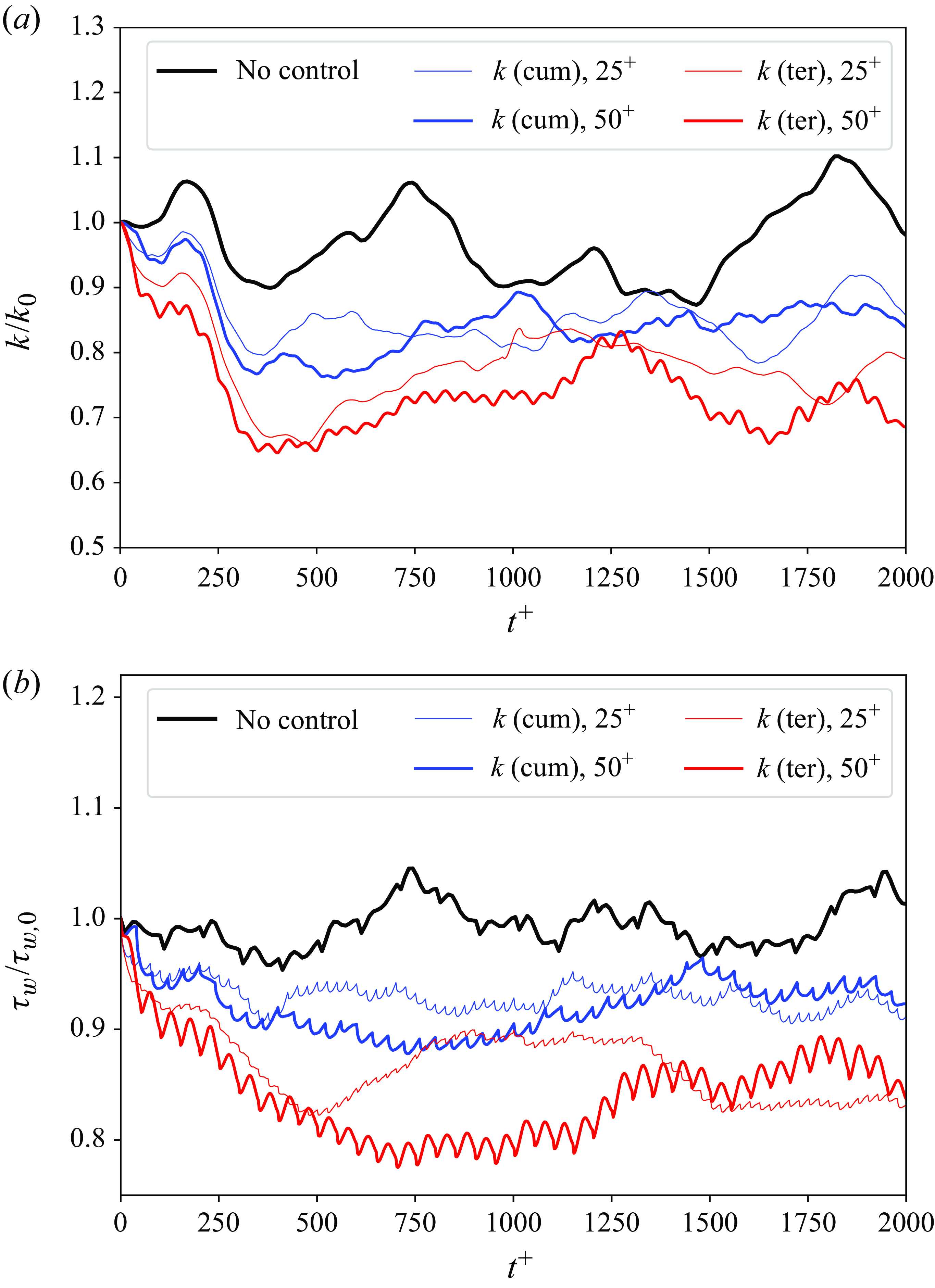
Figure 5. The history of (a) TKE $k$
and (b) wall friction
$k$
and (b) wall friction $\tau _w$
with opposition control targeting TKE related loss function. The legend follows the same format as figure 4, with
$\tau _w$
with opposition control targeting TKE related loss function. The legend follows the same format as figure 4, with $k$
denoting TKE control.
$k$
denoting TKE control.
3.1.2. The characteristic of control $\phi$

To gain deeper insights into the control mechanisms and the differences arising from varying control targets, we examine in more detail the optimised $\phi$
across all opposition control scenarios. Figure 6 provides a comparison of
$\phi$
across all opposition control scenarios. Figure 6 provides a comparison of $\phi$
fields in the wall friction control scenarios initialised under identical conditions. In the cases of cumulative wall friction control depicted in figure 6(a,c), the control fields
$\phi$
fields in the wall friction control scenarios initialised under identical conditions. In the cases of cumulative wall friction control depicted in figure 6(a,c), the control fields $\phi$
exhibit streamwise elongated structures, resembling the form of high- and low-speed streaks in the near-wall region (illustrated with isolines). When considering a longer time horizon, the control
$\phi$
exhibit streamwise elongated structures, resembling the form of high- and low-speed streaks in the near-wall region (illustrated with isolines). When considering a longer time horizon, the control $\phi$
shows longer streamwise structures. For terminal control
$\phi$
shows longer streamwise structures. For terminal control $\phi$
, the spanwise spacing of the streak-like formations matches that of the cumulative control
$\phi$
, the spanwise spacing of the streak-like formations matches that of the cumulative control $\phi$
, but these formations possess a shorter streamwise scale and greater magnitude.
$\phi$
, but these formations possess a shorter streamwise scale and greater magnitude.
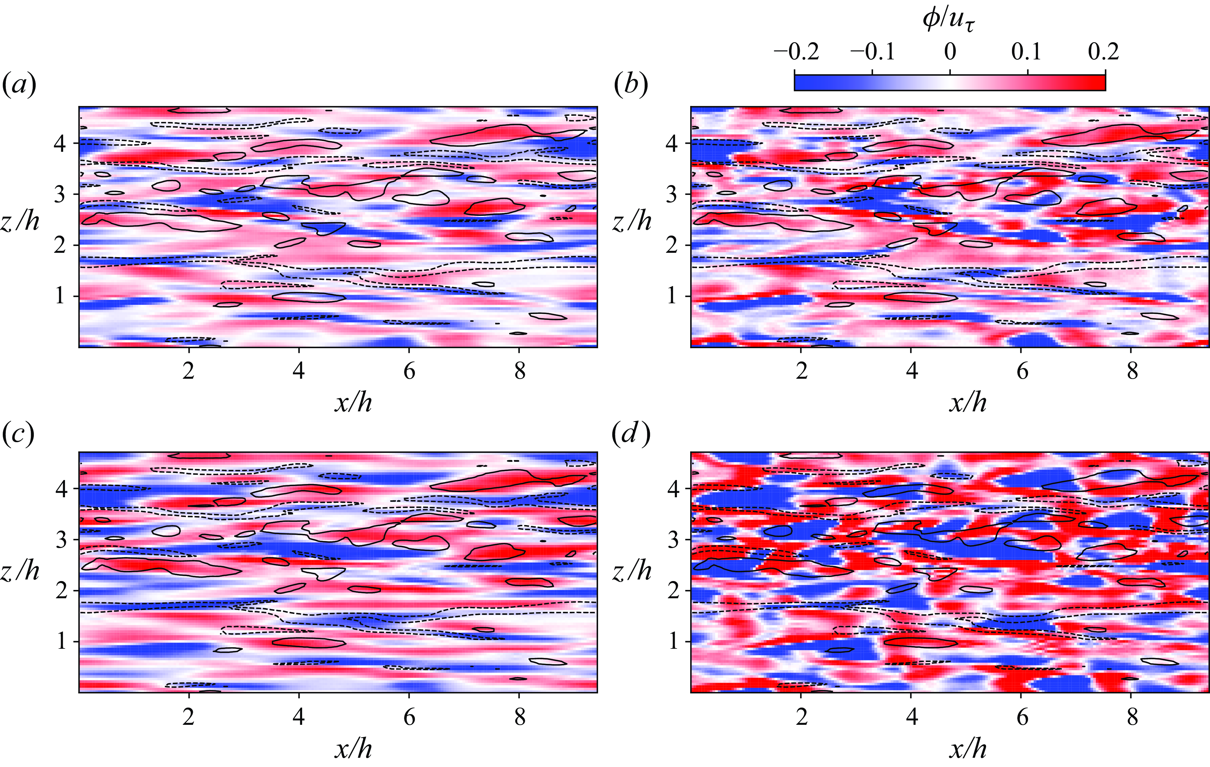
Figure 6. The opposition control $\phi (t^+=0)$
for wall friction control with different targets and time horizons. (a) Cumulative
$\phi (t^+=0)$
for wall friction control with different targets and time horizons. (a) Cumulative $\tau _w$
with
$\tau _w$
with $\Delta t^+=25$
; (b) terminal
$\Delta t^+=25$
; (b) terminal $\tau _w$
with
$\tau _w$
with $\Delta t^+=25$
; (c) cumulative
$\Delta t^+=25$
; (c) cumulative $\tau _w$
with
$\tau _w$
with $\Delta t^+=50$
; (d) terminal
$\Delta t^+=50$
; (d) terminal $\tau _w$
with
$\tau _w$
with $\Delta t^+=50$
. The isolines depict the initial
$\Delta t^+=50$
. The isolines depict the initial $u'$
of the episode at buffer layer (
$u'$
of the episode at buffer layer ( $y^+=15$
). The solid and dashed isolines indicate levels
$y^+=15$
). The solid and dashed isolines indicate levels $u'/\sigma _{u'}=-1$
and 1, respectively.
$u'/\sigma _{u'}=-1$
and 1, respectively.
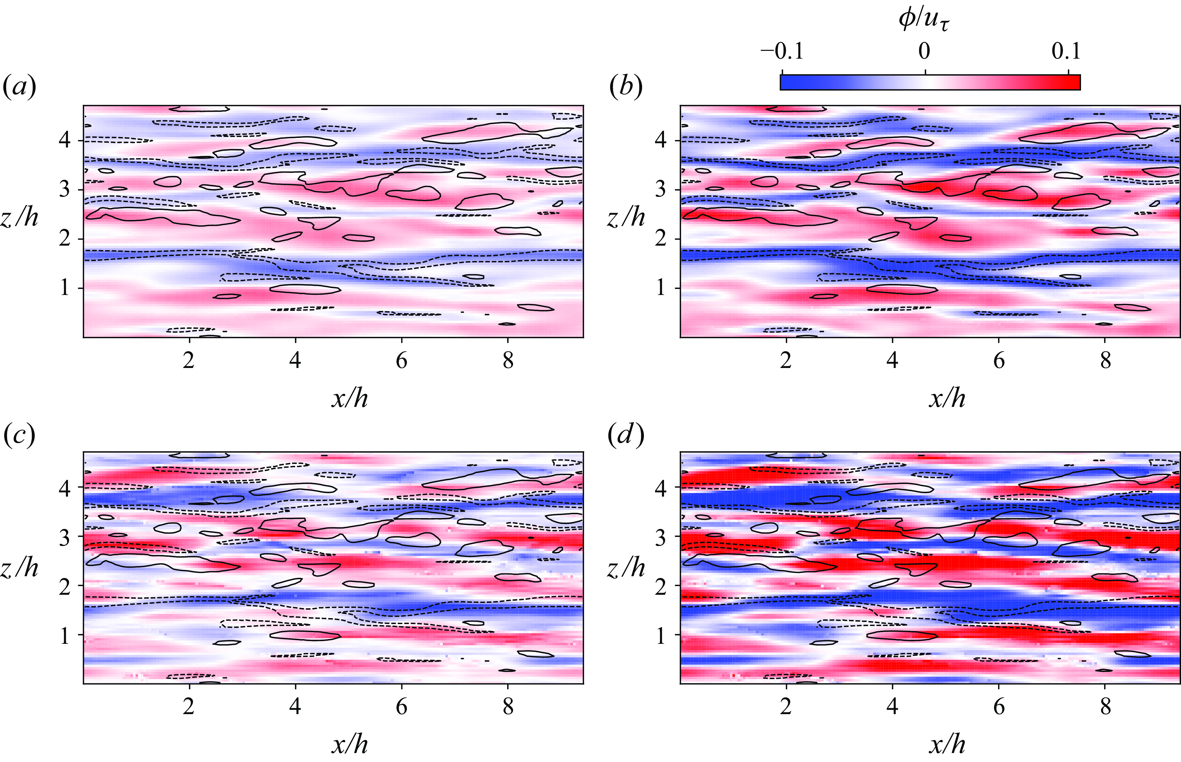
Figure 7. The opposition control $\phi (t^+=0)$
for TKE control with different targets and time horizons. (a) Cumulative
$\phi (t^+=0)$
for TKE control with different targets and time horizons. (a) Cumulative $k$
with
$k$
with $\Delta t^+=25$
; (b) terminal
$\Delta t^+=25$
; (b) terminal $k$
with
$k$
with $\Delta t^+=25$
; (c) cumulative
$\Delta t^+=25$
; (c) cumulative $k$
with
$k$
with $\Delta t^+=50$
; (d) terminal
$\Delta t^+=50$
; (d) terminal $k$
with
$k$
with $\Delta t^+=50$
. The isolines depict the initial
$\Delta t^+=50$
. The isolines depict the initial $u'$
of the episode at buffer layer (
$u'$
of the episode at buffer layer ( $y^+=15$
). The solid and dashed isolines indicate levels
$y^+=15$
). The solid and dashed isolines indicate levels $u'/\sigma _{u'}=-1$
and 1, respectively.
$u'/\sigma _{u'}=-1$
and 1, respectively.
The similarity of $\phi$
and the
$\phi$
and the $u'$
structures suggests that the form of
$u'$
structures suggests that the form of $\phi$
is intimately linked to the reduction of energetic structures near the wall. Additionally, for cumulative control
$\phi$
is intimately linked to the reduction of energetic structures near the wall. Additionally, for cumulative control $\phi$
, regions of upward momentum flux largely coincide with high-speed streaks (solid isolines in figure 6), whereas the areas of downward flux align with low-speed streaks (dashed isolines). This correlation generates a positive Reynolds stress
$\phi$
, regions of upward momentum flux largely coincide with high-speed streaks (solid isolines in figure 6), whereas the areas of downward flux align with low-speed streaks (dashed isolines). This correlation generates a positive Reynolds stress $\langle u'v'\rangle$
that acts against the original Reynolds stress in the flow. It is important to note that the
$\langle u'v'\rangle$
that acts against the original Reynolds stress in the flow. It is important to note that the $u'$
fields depicted with isolines in figure 6 represent the initial state of the optimisation episode. There is no clear correlation between the terminal control
$u'$
fields depicted with isolines in figure 6 represent the initial state of the optimisation episode. There is no clear correlation between the terminal control $\phi$
and the initial
$\phi$
and the initial $u'$
field because the terminal control is focused solely on the final outcome of the optimisation. Since near-wall friction velocity can be quickly adjusted by altering the boundary condition, the influence from the initial flow state to the terminal control
$u'$
field because the terminal control is focused solely on the final outcome of the optimisation. Since near-wall friction velocity can be quickly adjusted by altering the boundary condition, the influence from the initial flow state to the terminal control $\phi$
is anticipated to be minimal. It will be demonstrated subsequently that the terminal control
$\phi$
is anticipated to be minimal. It will be demonstrated subsequently that the terminal control $\phi$
displays a strong correlation with the terminal
$\phi$
displays a strong correlation with the terminal $u'$
fields.
$u'$
fields.
When compared with wall friction control, the TKE control fields $\phi$
display significant consistency across various loss functions (refer to figure 7). In all scenarios, the wall-normal flux in
$\phi$
display significant consistency across various loss functions (refer to figure 7). In all scenarios, the wall-normal flux in $\phi$
aligns closely with low- and high-speed streaks within the buffer layer (indicated by isolines). Specifically, the upward flux corresponds to regions of positive
$\phi$
aligns closely with low- and high-speed streaks within the buffer layer (indicated by isolines). Specifically, the upward flux corresponds to regions of positive $u'$
, whereas the downward flux is situated in areas of negative
$u'$
, whereas the downward flux is situated in areas of negative $u'$
. The impact of the duration of the time horizon is minimal. In cases with a longer time horizon, the coherent structures in control
$u'$
. The impact of the duration of the time horizon is minimal. In cases with a longer time horizon, the coherent structures in control $\phi$
are smoothed due to time-averaging effects, resulting in fewer small-scale details. Terminal control
$\phi$
are smoothed due to time-averaging effects, resulting in fewer small-scale details. Terminal control $\phi$
exhibits a greater magnitude compared with cumulative control
$\phi$
exhibits a greater magnitude compared with cumulative control $\phi$
, indicating a more aggressive control strategy.
$\phi$
, indicating a more aggressive control strategy.
Terminal TKE control’s similarity in control $\phi$
to cumulative TKE control supports our earlier discussion, indicating that loss functions involving terminal TKE implicitly encompass flow dynamics over the full time span. Consequently, even though the initial flow state is not directly included in the loss function, the control
$\phi$
to cumulative TKE control supports our earlier discussion, indicating that loss functions involving terminal TKE implicitly encompass flow dynamics over the full time span. Consequently, even though the initial flow state is not directly included in the loss function, the control $\phi$
closely resembles the energetic structures present within it.
$\phi$
closely resembles the energetic structures present within it.
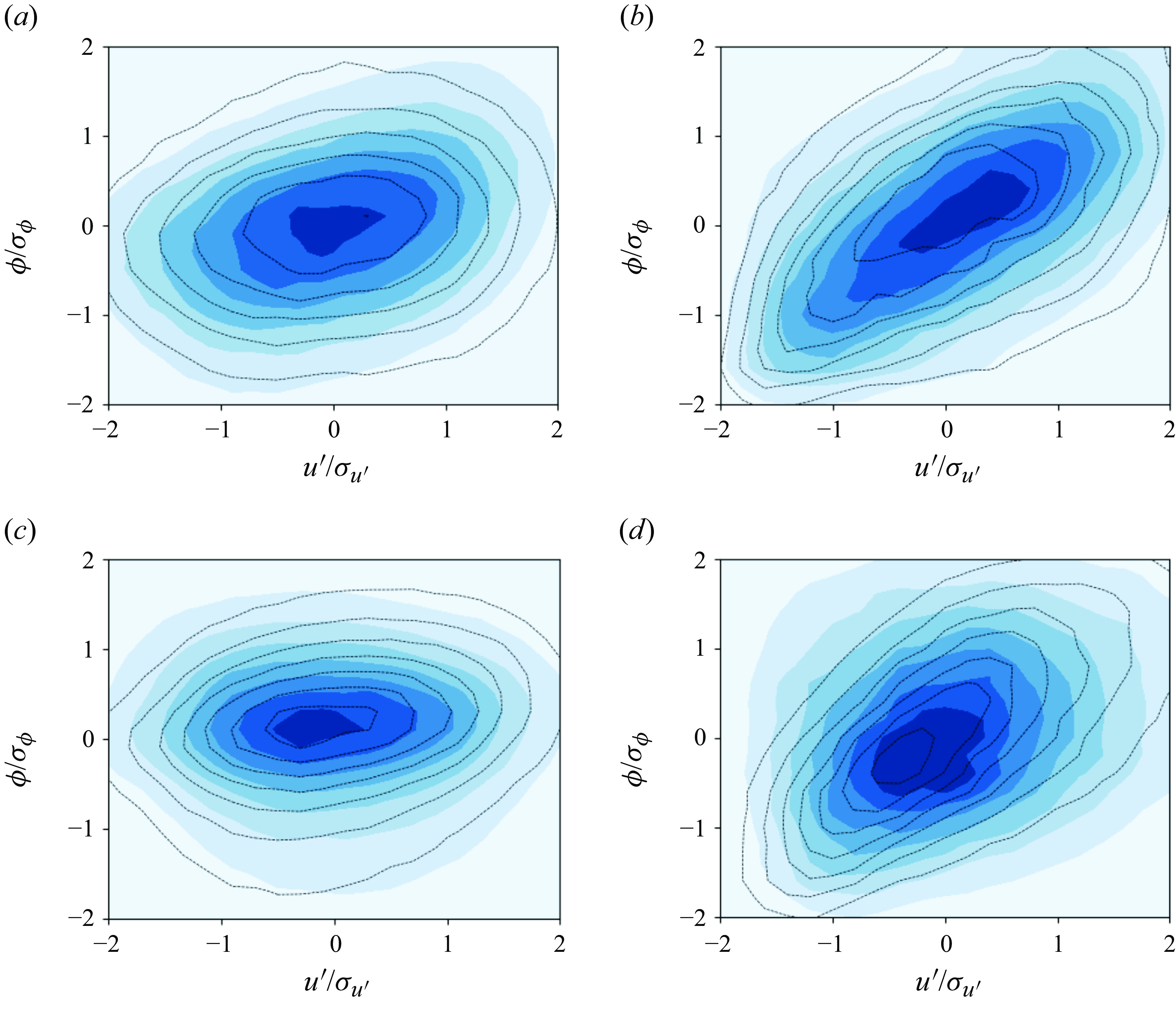
Figure 8. The joint PDF $f_{\phi u'}$
between control
$f_{\phi u'}$
between control $\phi$
and streamwise fluctuation
$\phi$
and streamwise fluctuation $u'$
at
$u'$
at $y^+=15$
. (a) Cumulative
$y^+=15$
. (a) Cumulative $\tau _w$
control with
$\tau _w$
control with $\Delta t^+=50$
; (b) cumulative
$\Delta t^+=50$
; (b) cumulative $k$
control with
$k$
control with $\Delta t^+=50$
; (c) terminal
$\Delta t^+=50$
; (c) terminal $\tau _w$
control with
$\tau _w$
control with $\Delta t^+=50$
; (d) terminal
$\Delta t^+=50$
; (d) terminal $k$
control with
$k$
control with $\Delta t^+=50$
. The coloured contours show the joint PDF
$\Delta t^+=50$
. The coloured contours show the joint PDF $f_{\phi u^{\prime}_{0}}$
between the control
$f_{\phi u^{\prime}_{0}}$
between the control $\phi$
and initial
$\phi$
and initial $u'$
, and the dashed isolines show the joint PDF
$u'$
, and the dashed isolines show the joint PDF $f_{\phi u^{\prime}_{\Delta t}}$
between the control
$f_{\phi u^{\prime}_{\Delta t}}$
between the control $\phi$
and terminal
$\phi$
and terminal $u'$
.
$u'$
.
To gain a deeper insight into the regulation mechanisms for different control objectives, figure 8 displays the joint probability density function (PDF) relating the control variable $\phi$
to
$\phi$
to $u'$
, highlighting their statistical association. For clarity, we illustrate only four typical scenarios with
$u'$
, highlighting their statistical association. For clarity, we illustrate only four typical scenarios with $\Delta t^+=50$
, as other cases with shorter intervals exhibit essentially the same pattern. In cumulative wall friction control (with
$\Delta t^+=50$
, as other cases with shorter intervals exhibit essentially the same pattern. In cumulative wall friction control (with $\Delta t^+=50$
, figure 8
a), the joint PDF
$\Delta t^+=50$
, figure 8
a), the joint PDF $f_{\phi u^{\prime}_{0}}$
(coloured contour) between
$f_{\phi u^{\prime}_{0}}$
(coloured contour) between $\phi$
and the initial streamwise fluctuation
$\phi$
and the initial streamwise fluctuation $u^{\prime}_{0}$
shows a distribution skewed towards the first and third quadrants, indicating a clear positive correlation. This aligns with our earlier findings in instantaneous flow fields (figure 6
c). The joint PDF
$u^{\prime}_{0}$
shows a distribution skewed towards the first and third quadrants, indicating a clear positive correlation. This aligns with our earlier findings in instantaneous flow fields (figure 6
c). The joint PDF $f_{\phi u^{\prime}_{\Delta t}}$
(dashed isolines) between
$f_{\phi u^{\prime}_{\Delta t}}$
(dashed isolines) between $\phi$
and the final
$\phi$
and the final $u^{\prime}_{\Delta t}$
exhibits a slightly weaker correlation compared with
$u^{\prime}_{\Delta t}$
exhibits a slightly weaker correlation compared with $f_{\phi u^{\prime}_{0}}$
. The positive correlation between
$f_{\phi u^{\prime}_{0}}$
. The positive correlation between $\phi$
and both the initial and final
$\phi$
and both the initial and final $u'$
corroborates that the cumulative control
$u'$
corroborates that the cumulative control $\phi$
achieved through the optimisation process considers minimising wall friction across the entire time horizon. Conversely, in terminal wall friction control (with
$\phi$
achieved through the optimisation process considers minimising wall friction across the entire time horizon. Conversely, in terminal wall friction control (with $\Delta t^+=50$
, figure 8
c), the joint PDF
$\Delta t^+=50$
, figure 8
c), the joint PDF $f_{\phi u^{\prime}_{0}}$
(coloured contour) is symmetric around
$f_{\phi u^{\prime}_{0}}$
(coloured contour) is symmetric around $u'=0$
, indicating that
$u'=0$
, indicating that $\phi$
is largely uncorrelated with the initial
$\phi$
is largely uncorrelated with the initial $u^{\prime}_{0}$
. This observation is consistent with figure 6(b). Regarding
$u^{\prime}_{0}$
. This observation is consistent with figure 6(b). Regarding $f_{\phi u^{\prime}_{\Delta t}}$
(dashed isolines), a distinct positive correlation is observed, confirming that terminal control of wall friction exclusively focuses on reducing friction at the terminal time.
$f_{\phi u^{\prime}_{\Delta t}}$
(dashed isolines), a distinct positive correlation is observed, confirming that terminal control of wall friction exclusively focuses on reducing friction at the terminal time.
The joint PDFs $f_{\phi u^{\prime}_{0}}$
and
$f_{\phi u^{\prime}_{0}}$
and $f_{\phi u^{\prime}_{\Delta t}}$
of cumulative TKE control depicted in figure 8(b) demonstrate a strong positive correlation between the control variable
$f_{\phi u^{\prime}_{\Delta t}}$
of cumulative TKE control depicted in figure 8(b) demonstrate a strong positive correlation between the control variable $\phi$
and both
$\phi$
and both $u^{\prime}_{0}$
and
$u^{\prime}_{0}$
and $u^{\prime}_{\Delta t}$
. In contrast with cumulative wall friction control, these distributions are more tightly centred around the line given by
$u^{\prime}_{\Delta t}$
. In contrast with cumulative wall friction control, these distributions are more tightly centred around the line given by $\phi /\sigma _\phi =u'/\sigma _{u'}$
, indicating a direct reliance of
$\phi /\sigma _\phi =u'/\sigma _{u'}$
, indicating a direct reliance of $\phi$
on
$\phi$
on $u'$
. Similarly, for terminal TKE control, control
$u'$
. Similarly, for terminal TKE control, control $\phi$
also displays a strong positive correlation with
$\phi$
also displays a strong positive correlation with $u^{\prime}_{\Delta t}$
. While
$u^{\prime}_{\Delta t}$
. While $\phi$
shows a weaker correlation with
$\phi$
shows a weaker correlation with $u^{\prime}_{0}$
, there is still a distinct skew of
$u^{\prime}_{0}$
, there is still a distinct skew of $f_{\phi u^{\prime}_{0}}$
towards the first and third quadrants. These observations align with the instantaneous field data shown in figure 7(b,d).
$f_{\phi u^{\prime}_{0}}$
towards the first and third quadrants. These observations align with the instantaneous field data shown in figure 7(b,d).
It is worth reiterating the distinction between terminal wall friction control and terminal TKE control. The control variable $\phi$
for the former has almost no correlation with the initial
$\phi$
for the former has almost no correlation with the initial $u^{\prime}_{0}$
condition, whereas the control
$u^{\prime}_{0}$
condition, whereas the control $\phi$
for the latter shows a notable correlation with
$\phi$
for the latter shows a notable correlation with $u^{\prime}_{0}$
. Although both scenarios only incorporate the terminal state in the loss function, this discrepancy arises from the inherent characteristics of the target, including spatial extent, wall location and related variables. Turbulent kinetic energy is an appealing option as it pertains to every component of turbulent velocity throughout the channel. Nonetheless, several issues remain unresolved, such as why friction control optimisation underperforms compared with TKE control, and what fundamentally differentiates the control strategies of wall friction and TKE control. These concerns will be addressed through a more detailed examination of the statistics of the turbulent channel.
$u^{\prime}_{0}$
. Although both scenarios only incorporate the terminal state in the loss function, this discrepancy arises from the inherent characteristics of the target, including spatial extent, wall location and related variables. Turbulent kinetic energy is an appealing option as it pertains to every component of turbulent velocity throughout the channel. Nonetheless, several issues remain unresolved, such as why friction control optimisation underperforms compared with TKE control, and what fundamentally differentiates the control strategies of wall friction and TKE control. These concerns will be addressed through a more detailed examination of the statistics of the turbulent channel.
3.1.3. The mean statistics
This section delves into the mean statistics of controlled flow fields to understand the control mechanisms aimed at different targets. Table 1 provides a summary of the wall friction coefficient $C_f$
for a standard turbulent channel, along with the relative changes
$C_f$
for a standard turbulent channel, along with the relative changes $\Delta C_f$
observed in the control scenarios. In each case, the skin friction is calculated using the flow fields over the time interval
$\Delta C_f$
observed in the control scenarios. In each case, the skin friction is calculated using the flow fields over the time interval $t^+=500-2000$
. Currently, our focus is on the overall wall friction coefficient, while the decomposition of wall friction will be addressed later in the section. With the exception of the terminal
$t^+=500-2000$
. Currently, our focus is on the overall wall friction coefficient, while the decomposition of wall friction will be addressed later in the section. With the exception of the terminal $\tau _w$
control cases, which exhibit a substantial rise in wall friction owing to instability, all opposition control methods result in varying levels of drag reduction. The differences in effectiveness across different control targets can be somewhat elucidated by examining the mean statistics.
$\tau _w$
control cases, which exhibit a substantial rise in wall friction owing to instability, all opposition control methods result in varying levels of drag reduction. The differences in effectiveness across different control targets can be somewhat elucidated by examining the mean statistics.
Table 1. The wall friction of the turbulent channel and the relative change in opposition control cases.
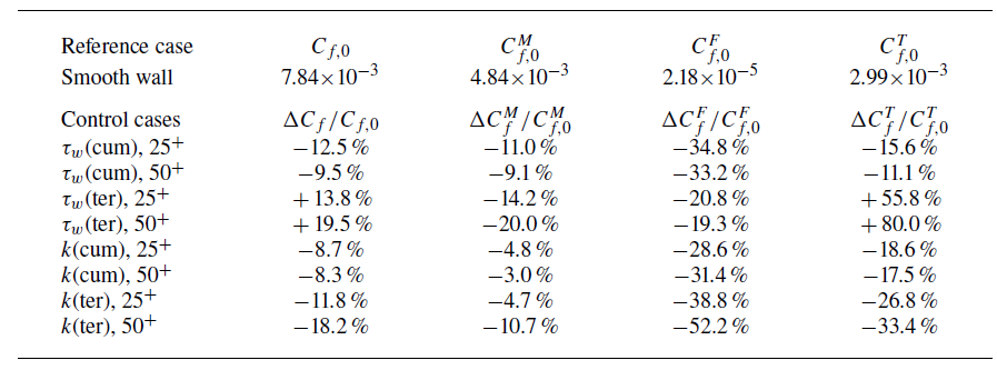
Figure 9(a) displays the average statistics for the four typical scenarios with $\Delta t^+=50$
, including both cumulative and terminal control of wall friction and TKE. The mean streamwise velocity profiles
$\Delta t^+=50$
, including both cumulative and terminal control of wall friction and TKE. The mean streamwise velocity profiles $\langle u\rangle /u_\tau$
(figure 9
a) show an upward shift in the outer region for all controlled cases when compared with the reference smooth wall scenario. This upward shift signifies a decrease in wall friction velocity
$\langle u\rangle /u_\tau$
(figure 9
a) show an upward shift in the outer region for all controlled cases when compared with the reference smooth wall scenario. This upward shift signifies a decrease in wall friction velocity $u_\tau$
, which is directly associated with wall shear stress
$u_\tau$
, which is directly associated with wall shear stress $\tau _w$
. This can be confirmed by comparing to table 1. The extent of drag reduction tends to correspond with the degree of shift in the
$\tau _w$
. This can be confirmed by comparing to table 1. The extent of drag reduction tends to correspond with the degree of shift in the $\langle u\rangle /u_\tau$
profile. From the extent of the shift, the terminal TKE control demonstrates superior performance in friction reduction among the four cases.
$\langle u\rangle /u_\tau$
profile. From the extent of the shift, the terminal TKE control demonstrates superior performance in friction reduction among the four cases.
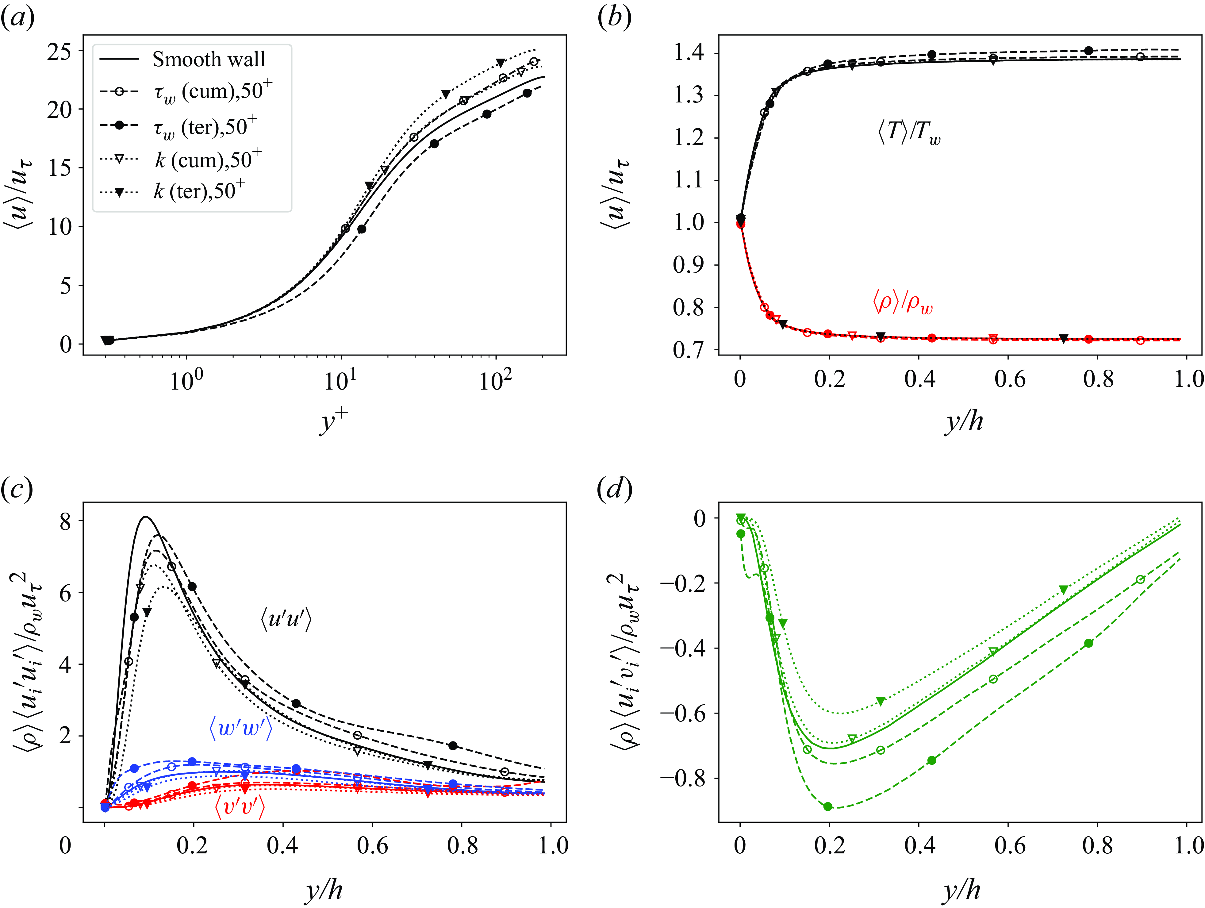
Figure 9. Mean statistics of opposition control cases compared with the smooth wall channel. (a) Mean streamwise velocity $\langle u\rangle$
; (b) mean temperature
$\langle u\rangle$
; (b) mean temperature $\langle T\rangle$
and mean density
$\langle T\rangle$
and mean density $\langle \rho \rangle$
; (c) turbulent intensity
$\langle \rho \rangle$
; (c) turbulent intensity $\langle u^{\prime}_{i}u^{\prime}_{i}\rangle$
; (d) Reynolds stress
$\langle u^{\prime}_{i}u^{\prime}_{i}\rangle$
; (d) Reynolds stress $\langle u'v'\rangle$
.
$\langle u'v'\rangle$
.
The average density $\langle \rho \rangle$
profiles (figure 9
a) in all cases remain largely unchanged, indicating that the compressibility of the channel is not affected by opposition control. Similarly, the temperature distribution
$\langle \rho \rangle$
profiles (figure 9
a) in all cases remain largely unchanged, indicating that the compressibility of the channel is not affected by opposition control. Similarly, the temperature distribution $\langle T\rangle$
within the channel exhibits minimal alteration. Only the case involving friction control of the terminal wall shows a slight increase in temperature in the central area of the channel, which could be related to the increase in viscous dissipation owing to a notable increase in the intensity of the turbulence (figure 9
c).
$\langle T\rangle$
within the channel exhibits minimal alteration. Only the case involving friction control of the terminal wall shows a slight increase in temperature in the central area of the channel, which could be related to the increase in viscous dissipation owing to a notable increase in the intensity of the turbulence (figure 9
c).
In the scenarios involving wall friction control, the peak of $\langle u'u' \rangle$
is seen to move farther from the wall. Although the peak closer to the wall decreases, there is an increase in
$\langle u'u' \rangle$
is seen to move farther from the wall. Although the peak closer to the wall decreases, there is an increase in $\langle u'u' \rangle$
within the outer region. Moreover, a notable rise in
$\langle u'u' \rangle$
within the outer region. Moreover, a notable rise in $\langle v'v' \rangle$
and
$\langle v'v' \rangle$
and $\langle w'w' \rangle$
is detected in the terminal friction control case. In contrast, for the TKE control cases,
$\langle w'w' \rangle$
is detected in the terminal friction control case. In contrast, for the TKE control cases, $\langle u'u' \rangle$
is not only significantly reduced near the wall but also maintains a low level in the outer region. Similarly,
$\langle u'u' \rangle$
is not only significantly reduced near the wall but also maintains a low level in the outer region. Similarly, $\langle v'v' \rangle$
and
$\langle v'v' \rangle$
and $\langle w'w' \rangle$
are diminished in TKE control cases.
$\langle w'w' \rangle$
are diminished in TKE control cases.
Similarly to the intensity of the turbulence, the Reynolds stress $\langle u'v' \rangle$
(figure 9
d) of
$\langle u'v' \rangle$
(figure 9
d) of $\tau _w$
control cases shows negligible reductions near the wall, yet it is considerably greater than in the smooth wall scenario in the outer region. In the TKE control cases, particularly with terminal control, the
$\tau _w$
control cases shows negligible reductions near the wall, yet it is considerably greater than in the smooth wall scenario in the outer region. In the TKE control cases, particularly with terminal control, the $\langle u'v' \rangle$
magnitude are notably lower than the baseline level.
$\langle u'v' \rangle$
magnitude are notably lower than the baseline level.
Analysis of the average statistics indicates a fundamental contrast in the approaches of wall friction control versus TKE targeted control. In cases aimed at controlling wall friction, energetic turbulent structures such as streaks and vortices are displaced from the wall, resulting in an outward shift of the turbulence intensity and Reynolds stress peaks. Although this method may be temporarily effective, it induces additional turbulence fluctuations in the outer regions, ultimately enhancing the mixing and undermining the friction reduction efforts. Conversely, TKE control not only relocates the turbulence but also suppresses it without creating additional disturbances. The different tactics employed by the two control targets are related to the scope of their information. Wall friction control focuses solely on wall-specific data and lacks insight into outer region dynamics. Consequently, its optimal strategy is to push the friction-inducing structures away. Turbulent kinetic energy control retains well-rounded information across the entire channel, allowing it to successfully mitigate turbulence while avoiding any adverse effects.
3.1.4. Decomposition of wall friction
To further understand the change of friction source in different control cases, we apply skin-friction drag decomposition for compressible channel flow proposed by Renard & Deck (Reference Renard and Deck2016) and Li et al. (Reference Li, Fan, Modesti and Cheng2019):
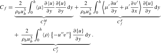 \begin{eqnarray}C_f &=& \underbrace {\frac {2}{\rho _b u_b^3} \int _0^h\langle \mu \rangle \frac {\partial \langle u\rangle }{\partial y} \frac {\partial \{u\}}{\partial y} \textrm {d} y}_{C_{f}^M}+\underbrace {\frac {2}{\rho _b u_b^3} \int _0^h\left \langle \mu ^{\prime } \frac {\partial u^{\prime }}{\partial y}+\mu ^{\prime } \frac {\partial v^{\prime }}{\partial x}\right \rangle \frac {\partial \{u\}}{\partial y} \textrm {d} y}_{C_{f}^F} \nonumber\\ && + \underbrace {\frac {2}{\rho _b u_b^3} \int _0^h\langle \rho \rangle \left \{-u^{\prime \prime } v^{\prime \prime }\right \} \frac {\partial \{u\}}{\partial y} \textrm {d} y}_{C_{f}^T}. \end{eqnarray}
Here $C_f^M$
and
$C_f^M$
and $C_f^F$
are both related to the direct molecular viscous dissipation, which transforms the power of the skin-friction drag into heat;
$C_f^F$
are both related to the direct molecular viscous dissipation, which transforms the power of the skin-friction drag into heat; $C_f^M$
is dependent on the mean shearing in the flow and
$C_f^M$
is dependent on the mean shearing in the flow and $C_f^F$
is generated due to the thermodynamic fluctuations in the compressible flow,
$C_f^F$
is generated due to the thermodynamic fluctuations in the compressible flow, $C_f^T$
represents the power converted into the production of TKE induced by turbulent fluctuations.
$C_f^T$
represents the power converted into the production of TKE induced by turbulent fluctuations.
Although this decomposition was originally formulated based on the no-slip wall condition, it is also applicable to opposition control with zero net flux at the wall. For all the cases, the residual error of RD identity is below $\pm 2.3\%$
. The RD identities for all cases are documented in table 1. Across all scenarios, the primary contributors are
$\pm 2.3\%$
. The RD identities for all cases are documented in table 1. Across all scenarios, the primary contributors are $C_f^M$
and
$C_f^M$
and $C_f^T$
, while the contribution from the compressibility effect of the flow,
$C_f^T$
, while the contribution from the compressibility effect of the flow, $C_f^F$
, is minimal due to the low Mach number. Figure 10 presents a comparison between the premultiplied integrands of the four typical cases (as in figure 8 and 9) and a smooth wall channel.
$C_f^F$
, is minimal due to the low Mach number. Figure 10 presents a comparison between the premultiplied integrands of the four typical cases (as in figure 8 and 9) and a smooth wall channel.
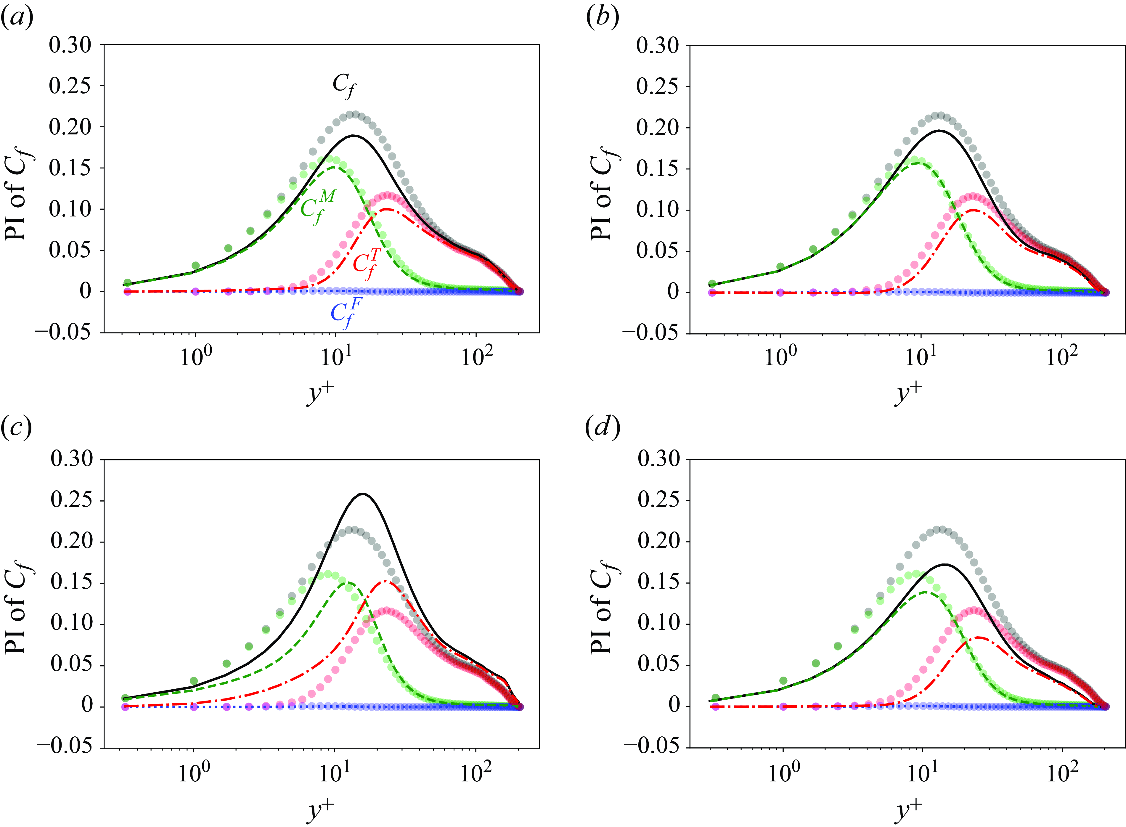
Figure 10. Premultiplied integrands (PI) of RD identity as a function of $y^+$
in opposition control cases. Here
$y^+$
in opposition control cases. Here $C_f^M$
,
$C_f^M$
, $C_f^F$
and
$C_f^F$
and $C_f^T$
are denoted by dashed lines, dotted lines and dash-dotted lines, respectively. The PIs of smooth wall channel are superimposed with circles. (a) Cumulative
$C_f^T$
are denoted by dashed lines, dotted lines and dash-dotted lines, respectively. The PIs of smooth wall channel are superimposed with circles. (a) Cumulative $\tau _w$
control,
$\tau _w$
control, $\Delta t^+=50$
; (b) cumulative
$\Delta t^+=50$
; (b) cumulative $k$
control,
$k$
control, $\Delta t^+=50$
; (c) terminal
$\Delta t^+=50$
; (c) terminal $\tau _w$
control,
$\tau _w$
control, $\Delta t^+=50$
; (d) terminal
$\Delta t^+=50$
; (d) terminal $k$
control,
$k$
control, $\Delta t^+=50$
.
$\Delta t^+=50$
.
In the case of cumulative $\tau _w$
control with
$\tau _w$
control with $\Delta t^+=50$
(figure 10
a), there is an approximate 10 % decrease in both
$\Delta t^+=50$
(figure 10
a), there is an approximate 10 % decrease in both $C_f^M$
and
$C_f^M$
and $C_f^T$
. The decrease in
$C_f^T$
. The decrease in $C_f^T$
is related to the positive correlation between the control parameter
$C_f^T$
is related to the positive correlation between the control parameter $\phi$
and the fluctuating velocity
$\phi$
and the fluctuating velocity $u'$
, as illustrated in figure 8(a). The decrease in
$u'$
, as illustrated in figure 8(a). The decrease in $C_f^M$
suggests alterations in the mean shear close to the wall, particularly for
$C_f^M$
suggests alterations in the mean shear close to the wall, particularly for $y^+$
below 10. This change is so subtle that it is not prominently observable in instantaneous flow fields (figure 3
a,c,e) or the normalised mean velocity profile (figure 9
a). The terminal
$y^+$
below 10. This change is so subtle that it is not prominently observable in instantaneous flow fields (figure 3
a,c,e) or the normalised mean velocity profile (figure 9
a). The terminal $\tau _w$
control (figure 10
c) more intensely altered the mean flow near the wall, decreasing
$\tau _w$
control (figure 10
c) more intensely altered the mean flow near the wall, decreasing $C_f^M$
by 20 %. However, the additional fluctuations it induced considerably amplified turbulent production, increasing
$C_f^M$
by 20 %. However, the additional fluctuations it induced considerably amplified turbulent production, increasing $C_f^T$
by 80 %. Consequently, its impact on mean shear at the wall is completely cancelled by increased turbulence, leading to increased wall friction.
$C_f^T$
by 80 %. Consequently, its impact on mean shear at the wall is completely cancelled by increased turbulence, leading to increased wall friction.
In the cumulative $k$
control illustrated in figure 9(b), the integrand of
$k$
control illustrated in figure 9(b), the integrand of $C_f^T$
is primarily reduced in the near-wall region (
$C_f^T$
is primarily reduced in the near-wall region ( $y^+\lt 30$
), while
$y^+\lt 30$
), while $C_f^M$
remains mostly unaffected. Conversely, the terminal
$C_f^M$
remains mostly unaffected. Conversely, the terminal $k$
control takes a notably more aggressive approach, significantly diminishing turbulence production near the wall and in the outer region, resulting in a 33.4 % decrease in
$k$
control takes a notably more aggressive approach, significantly diminishing turbulence production near the wall and in the outer region, resulting in a 33.4 % decrease in $C_f^T$
. Additionally, the mean shear on the wall undergoes a considerable decline. The effective reduction in both
$C_f^T$
. Additionally, the mean shear on the wall undergoes a considerable decline. The effective reduction in both $C_f^T$
and
$C_f^T$
and $C_f^M$
positions this as the most efficient opposition control strategy achieved through the current optimisation.
$C_f^M$
positions this as the most efficient opposition control strategy achieved through the current optimisation.
The findings from RD identity support our previous hypothesis on the distinct mechanisms employed in $\tau _w$
targeting control as opposed to
$\tau _w$
targeting control as opposed to $k$
targeting control. In cases of
$k$
targeting control. In cases of $\tau _w$
control, which only use limited data at the wall, the strategy tends to reduce shear at the wall, albeit at the cost of introducing flow disturbances. In contrast,
$\tau _w$
control, which only use limited data at the wall, the strategy tends to reduce shear at the wall, albeit at the cost of introducing flow disturbances. In contrast, $k$
control cases, equipped with a comprehensive dynamic flow profile within the loss function, adopt a turbulence cancellation strategy. The latter approach is evidently more efficient.
$k$
control cases, equipped with a comprehensive dynamic flow profile within the loss function, adopt a turbulence cancellation strategy. The latter approach is evidently more efficient.
It is noted that the maximum amplitude of $\phi /u_\tau$
is only in the order of
$\phi /u_\tau$
is only in the order of $\mathcal{O}$
(0.1), which is equivalent to
$\mathcal{O}$
(0.1), which is equivalent to $\phi /U_b\sim {\mathcal {O}}(10^{-3}$
). Therefore, the amount of kinetic energy flux carried by the control velocity is extremely low, which is attributed to a strong penalty for input energy in the loss functions. This could explain the relatively lower drag reduction rates in current cases, compared with the 23 % reduction reported by Yao & Hussain (Reference Yao and Hussain2021) where
$\phi /U_b\sim {\mathcal {O}}(10^{-3}$
). Therefore, the amount of kinetic energy flux carried by the control velocity is extremely low, which is attributed to a strong penalty for input energy in the loss functions. This could explain the relatively lower drag reduction rates in current cases, compared with the 23 % reduction reported by Yao & Hussain (Reference Yao and Hussain2021) where $\phi /u_\tau$
is estimated to be
$\phi /u_\tau$
is estimated to be $\mathcal {O}$
(1). In addition, the low update frequency of the control field also limits the performance. Nevertheless, the control field generated by the optimisation process has a valid physics interpretation that aligns with the mechanism of opposition control (Rebbeck & Choi Reference Rebbeck and Choi2006). This validates the effectiveness and convergence of the Adam algorithm in searching for control solutions within the current optimisation framework. The significant performance disparity between cases also highlights that, despite auto-differentiation enabling swift gradient computation with numerous parameters, the results are predominantly determined by the choice of loss function, which should be grounded in physical insights.
$\mathcal {O}$
(1). In addition, the low update frequency of the control field also limits the performance. Nevertheless, the control field generated by the optimisation process has a valid physics interpretation that aligns with the mechanism of opposition control (Rebbeck & Choi Reference Rebbeck and Choi2006). This validates the effectiveness and convergence of the Adam algorithm in searching for control solutions within the current optimisation framework. The significant performance disparity between cases also highlights that, despite auto-differentiation enabling swift gradient computation with numerous parameters, the results are predominantly determined by the choice of loss function, which should be grounded in physical insights.
3.2. The performance of tunable permeable wall
The main drawback of opposition control, similar to other active control techniques, is its high energy consumption. Consequently, passive control strategies continue to be widely intriguing for industrial implementation. In this research, we investigate the effectiveness of a permeable wall for drag reduction. Prior research has indicated that a stationary permeable wall can reduce drag if the permeability is extremely low and predominantly aligned in the streamwise direction (Rosti et al. Reference Rosti, Brandt and Pinelli2018). Aside from this specific instance, most studies on permeable walls have noted an increase in drag (Abderrahaman-Elena & García-Mayoral Reference Abderrahaman-Elena and García-Mayoral2017; Wang et al. Reference Wang, Chu, Lozano-Durán, Helmig and Weigand2021a , Reference Wang, Yang, Evrim, Terzis, Helmig and Chub ). We are now removing the temporal invariance constraint on the permeable wall to allow the permeability to vary with each optimisation cycle. Although walls with tunable permeability are not frequently explored, it can be implemented using metamaterials (Zheng et al. Reference Zheng2014), a shape memory polymer (Santo Reference Santo2016), or stimuli-responsive materials (Wei et al. Reference Wei, Gao, Li and Serpe2017).
In each optimisation episode, we adjust the boundary condition parameter ( $\beta$
for the permeable wall) according to our control objectives. Unlike opposition control, where constant energy put is necessary, tunable porous materials such as metamaterials, shape memory foams and stimuli-responsive polymers only require energy during the state-changing phase. After the porosity adjustment is done, no extra energy is needed to preserve the changed state, moving the porous material into a ‘passive control’ mode. Since we overlook the energy required for state change, the tunable permeable wall has the advantage that there is no energy input constraint in the loss function. However, the permeable wall lacks the ability to add or remove mass directly from the flow as opposition control. Instead, it can only modulate local flux through changes in local permeability, which may considerably limit its ability to alter the channel. Therefore, it is intriguing to explore whether the high degrees of freedom offered by tunable permeability can be used to achieve drag reduction.
$\beta$
for the permeable wall) according to our control objectives. Unlike opposition control, where constant energy put is necessary, tunable porous materials such as metamaterials, shape memory foams and stimuli-responsive polymers only require energy during the state-changing phase. After the porosity adjustment is done, no extra energy is needed to preserve the changed state, moving the porous material into a ‘passive control’ mode. Since we overlook the energy required for state change, the tunable permeable wall has the advantage that there is no energy input constraint in the loss function. However, the permeable wall lacks the ability to add or remove mass directly from the flow as opposition control. Instead, it can only modulate local flux through changes in local permeability, which may considerably limit its ability to alter the channel. Therefore, it is intriguing to explore whether the high degrees of freedom offered by tunable permeability can be used to achieve drag reduction.
Similarly to opposition control, there are several key factors to take into account here, such as the target variable (wall friction $\tau _w$
or TKE
$\tau _w$
or TKE $k$
), the type of loss function (whether cumulative or terminal) and the chosen time horizon (
$k$
), the type of loss function (whether cumulative or terminal) and the chosen time horizon ( $\Delta t^+=25$
or
$\Delta t^+=25$
or $\Delta t^+=50$
). To illustrate the evolution of turbulent structures over a permeable wall, figure 11 presents the instantaneous vorticity structures for two representative scenarios: cumulative
$\Delta t^+=50$
). To illustrate the evolution of turbulent structures over a permeable wall, figure 11 presents the instantaneous vorticity structures for two representative scenarios: cumulative $\tau _w$
control with
$\tau _w$
control with $\Delta t^+=25$
and terminal
$\Delta t^+=25$
and terminal $k$
control with
$k$
control with $\Delta t^+=25$
. The flow within the channel undergoes substantial alteration by intermittently varying the distribution of
$\Delta t^+=25$
. The flow within the channel undergoes substantial alteration by intermittently varying the distribution of $\beta$
(represented by the grey contour on the plane
$\beta$
(represented by the grey contour on the plane $y=0$
). For the cumulative
$y=0$
). For the cumulative $\tau _w$
control case (figure 11
a,c,e), the turbulence is intensified with an obvious increase in the population of vortices. Correspondingly, there is an increase in Reynolds stress (red solid line in plane
$\tau _w$
control case (figure 11
a,c,e), the turbulence is intensified with an obvious increase in the population of vortices. Correspondingly, there is an increase in Reynolds stress (red solid line in plane $z=0$
). In the terminal
$z=0$
). In the terminal $k$
control case (figure 11
b,d,f), the number of vortices in the fields is slightly reduced. This is also evidenced by the decrease of Reynolds stress (red solid line in plane
$k$
control case (figure 11
b,d,f), the number of vortices in the fields is slightly reduced. This is also evidenced by the decrease of Reynolds stress (red solid line in plane $z=0$
) in the outer region.
$z=0$
) in the outer region.
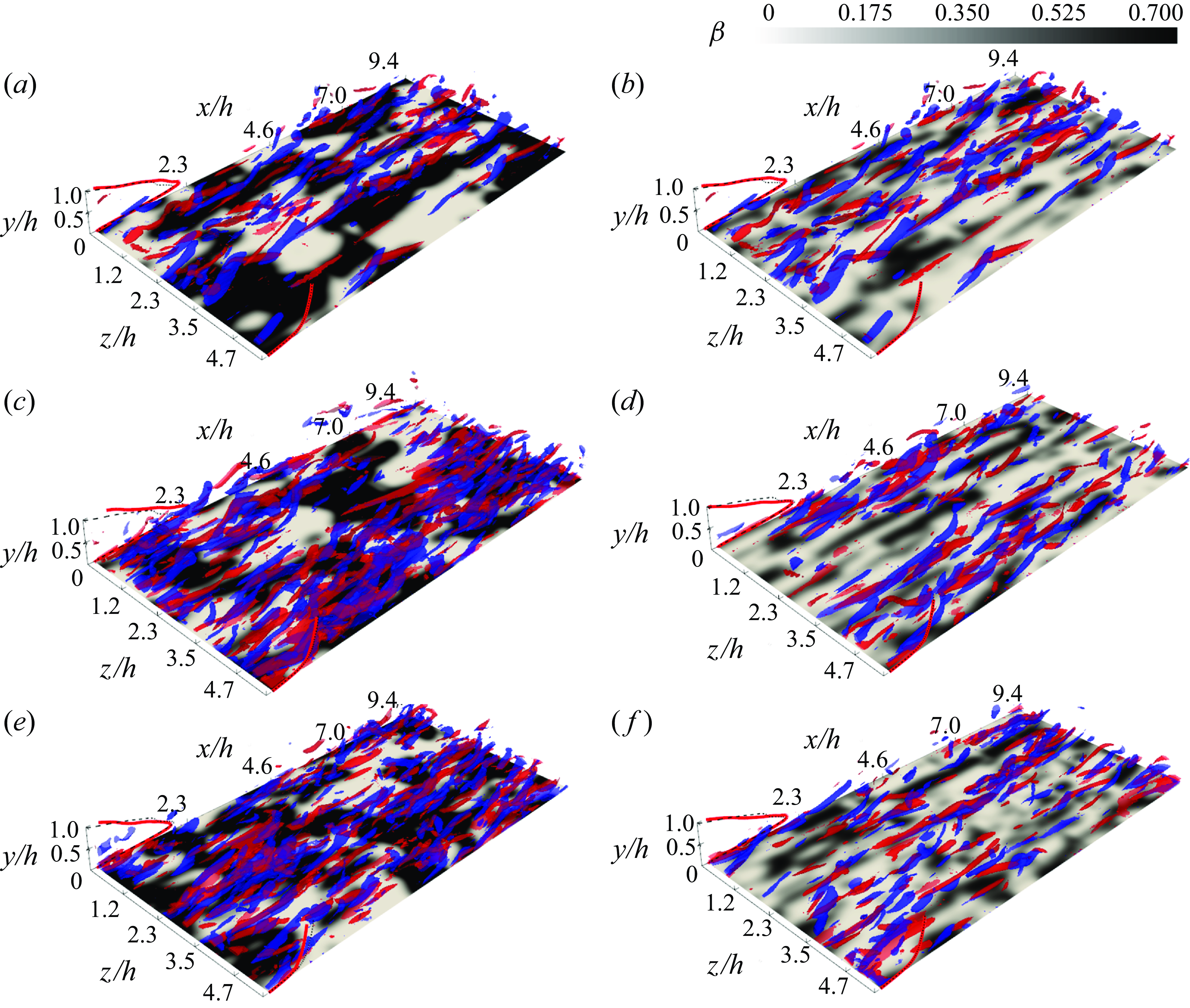
Figure 11. Vorticity structures above a tunable permeable wall. Panels (a,c,e) show cumulative wall friction control with $\Delta t^+=25$
, while panels (b,d,f) depict terminal TKE control with the same
$\Delta t^+=25$
, while panels (b,d,f) depict terminal TKE control with the same $\Delta t^+$
. The pairs of panels (a,b), (c,d) and (e,f) represent
$\Delta t^+$
. The pairs of panels (a,b), (c,d) and (e,f) represent $t^+=50$
,
$t^+=50$
, $t^+=500$
and
$t^+=500$
and $t^+=2000$
from the onset of control, respectively. Blue and red isosurfaces indicate streamwise vorticity at
$t^+=2000$
from the onset of control, respectively. Blue and red isosurfaces indicate streamwise vorticity at $\omega _x=\pm \sigma _{\omega _x}$
,
$\omega _x=\pm \sigma _{\omega _x}$
, $\sigma _{\omega _x}$
being the standard deviation of
$\sigma _{\omega _x}$
being the standard deviation of $\omega _x$
at
$\omega _x$
at $t=0$
. Control
$t=0$
. Control $\phi$
is illustrated on the wall with coloured contours. Present snapshot profiles of
$\phi$
is illustrated on the wall with coloured contours. Present snapshot profiles of $\langle u\rangle$
and
$\langle u\rangle$
and $-\langle u'v'\rangle$
are overlaid on front (
$-\langle u'v'\rangle$
are overlaid on front ( $z=1.5\pi$
) and back (
$z=1.5\pi$
) and back ( $z=0$
) planes with solid red lines. Black dashed lines show profiles from the smooth wall scenario for comparison. See also supplementary movies 3 and 4 for the full simulation duration.
$z=0$
) planes with solid red lines. Black dashed lines show profiles from the smooth wall scenario for comparison. See also supplementary movies 3 and 4 for the full simulation duration.
The $\beta$
fields (depicted as grey contours on the
$\beta$
fields (depicted as grey contours on the $y=0$
plane) predominantly exhibit two distinct values. For most parts of the wall, the local
$y=0$
plane) predominantly exhibit two distinct values. For most parts of the wall, the local $\beta$
registers either as 0, indicating non-permeability, or 0.7, which represents the upper bound for
$\beta$
registers either as 0, indicating non-permeability, or 0.7, which represents the upper bound for $\beta$
in the current optimisation study. Regions exhibiting
$\beta$
in the current optimisation study. Regions exhibiting $\beta$
values in between these extremes are relatively small. In the scenario of cumulative
$\beta$
values in between these extremes are relatively small. In the scenario of cumulative $\tau _w$
control (see figure 11
a,c,e), the permeable zone forms an interconnected network covering a substantial portion of the wall. Conversely, for the terminal
$\tau _w$
control (see figure 11
a,c,e), the permeable zone forms an interconnected network covering a substantial portion of the wall. Conversely, for the terminal $k$
control case, the permeable zones appear more segregated and streak like. A notable increase in intermediate
$k$
control case, the permeable zones appear more segregated and streak like. A notable increase in intermediate $\beta$
values suggests the need for more refined controls to manage turbulence. These distinctions in the patterns of the
$\beta$
values suggests the need for more refined controls to manage turbulence. These distinctions in the patterns of the $\beta$
map controls highlight fundamentally different control mechanisms between the
$\beta$
map controls highlight fundamentally different control mechanisms between the $\tau _w$
and
$\tau _w$
and $k$
control scenarios. Further discussion of these differences will be provided in the subsequent sections.
$k$
control scenarios. Further discussion of these differences will be provided in the subsequent sections.
3.2.1. The development of wall friction on tunable permeable walls
Figure 12 presents the progression of wall friction under the influence of wall friction control. With the permeable wall boundary condition, both cumulative and terminal $\tau _w$
control achieve stable outcomes in drag reduction, even in the terminal control scenarios. Notably, cumulative
$\tau _w$
control achieve stable outcomes in drag reduction, even in the terminal control scenarios. Notably, cumulative $\tau _w$
control with a time horizon
$\tau _w$
control with a time horizon $\Delta t^+=25$
achieves over 10 % drag reduction, while other control scenarios yield roughly a 5 % reduction.
$\Delta t^+=25$
achieves over 10 % drag reduction, while other control scenarios yield roughly a 5 % reduction.
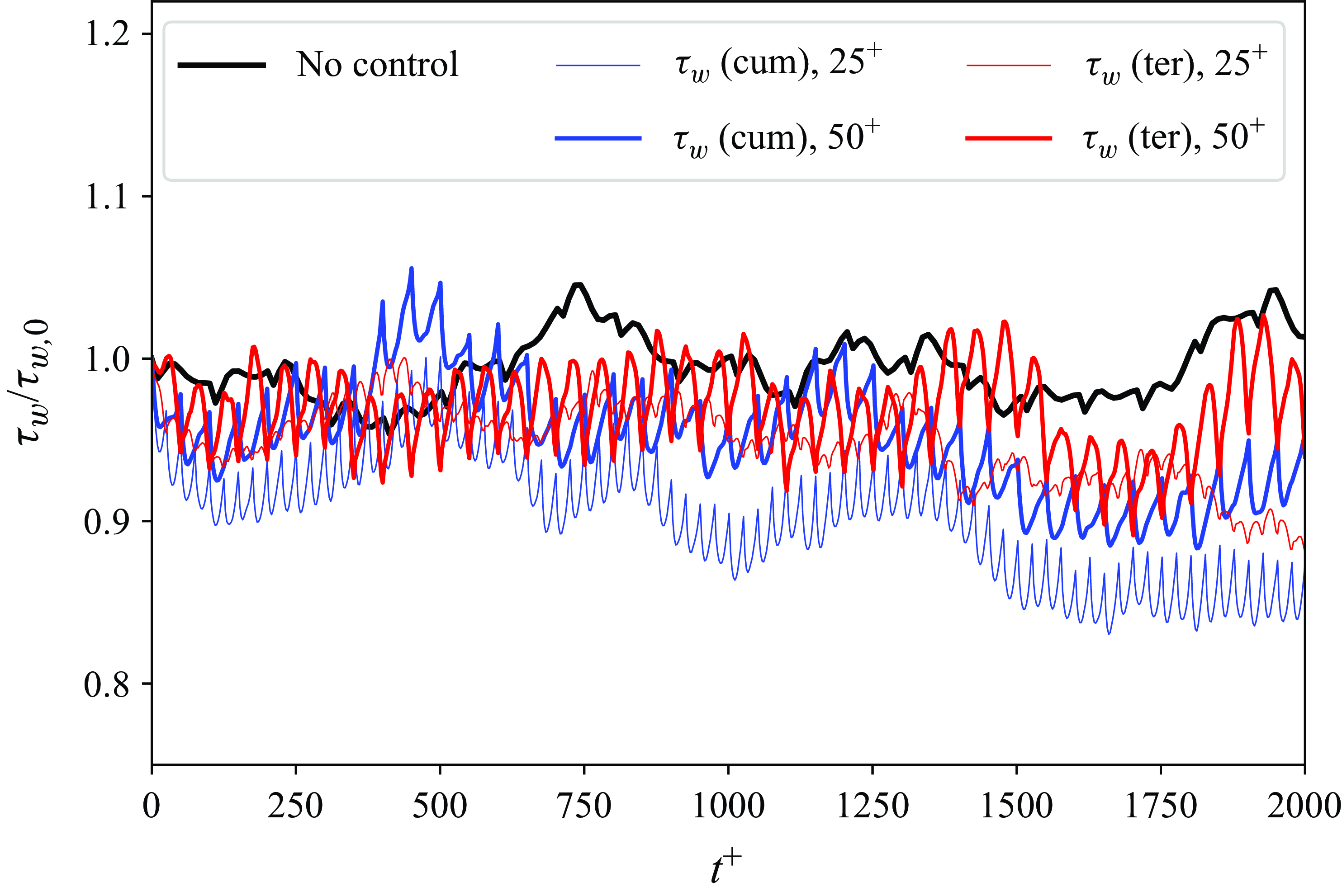
Figure 12. History of wall friction over tunable permeable wall targeting loss functions associated with $\tau _w$
.
$\tau _w$
.
It is noteworthy that the permeable wall, despite its lack of active flow manipulation ability like opposition control, possesses an advantage in maintaining stable control outputs with terminal control, relying on minimal information from the near-wall position. This is partly due to the special properties of disturbances generated by the permeable wall. The wall-normal flux at the permeable boundary is restricted to be proportional to the pressure fluctuations, which are mostly chaotic, with an upper limit for $\beta$
set at 0.7. These conditions ensure that the wall-normal flux remains limited and prevents excessive interfacial flux. Moreover, the drag reduction mechanism of the permeable wall differs from that used in opposition control, a topic to be further discussed in a subsequent section.
$\beta$
set at 0.7. These conditions ensure that the wall-normal flux remains limited and prevents excessive interfacial flux. Moreover, the drag reduction mechanism of the permeable wall differs from that used in opposition control, a topic to be further discussed in a subsequent section.
In the case of TKE control, the use of permeable walls proves to be less efficient than opposition control. Figure 13 illustrates the TKE and wall friction over time with permeable wall intervention. Generally, the reduction in TKE and wall friction is insignificant. The most successful scenario is terminal $k$
control with
$k$
control with $\Delta t^+=50$
, achieving around 5 % suppression in TKE and a 2 % reduction in drag. It is not surprising that the permeable wall is ineffective at controlling TKE. The current permeable wall boundary condition only includes a wall-normal component. Previous studies (Rosti et al. Reference Rosti, Brandt and Pinelli2018) have indicated that even slight wall-normal permeability can considerably enhance turbulence production and wall friction. Nevertheless, we demonstrate that reducing TKE and drag is indeed achievable through an optimised and adjustable distribution of
$\Delta t^+=50$
, achieving around 5 % suppression in TKE and a 2 % reduction in drag. It is not surprising that the permeable wall is ineffective at controlling TKE. The current permeable wall boundary condition only includes a wall-normal component. Previous studies (Rosti et al. Reference Rosti, Brandt and Pinelli2018) have indicated that even slight wall-normal permeability can considerably enhance turbulence production and wall friction. Nevertheless, we demonstrate that reducing TKE and drag is indeed achievable through an optimised and adjustable distribution of $\beta$
.
$\beta$
.
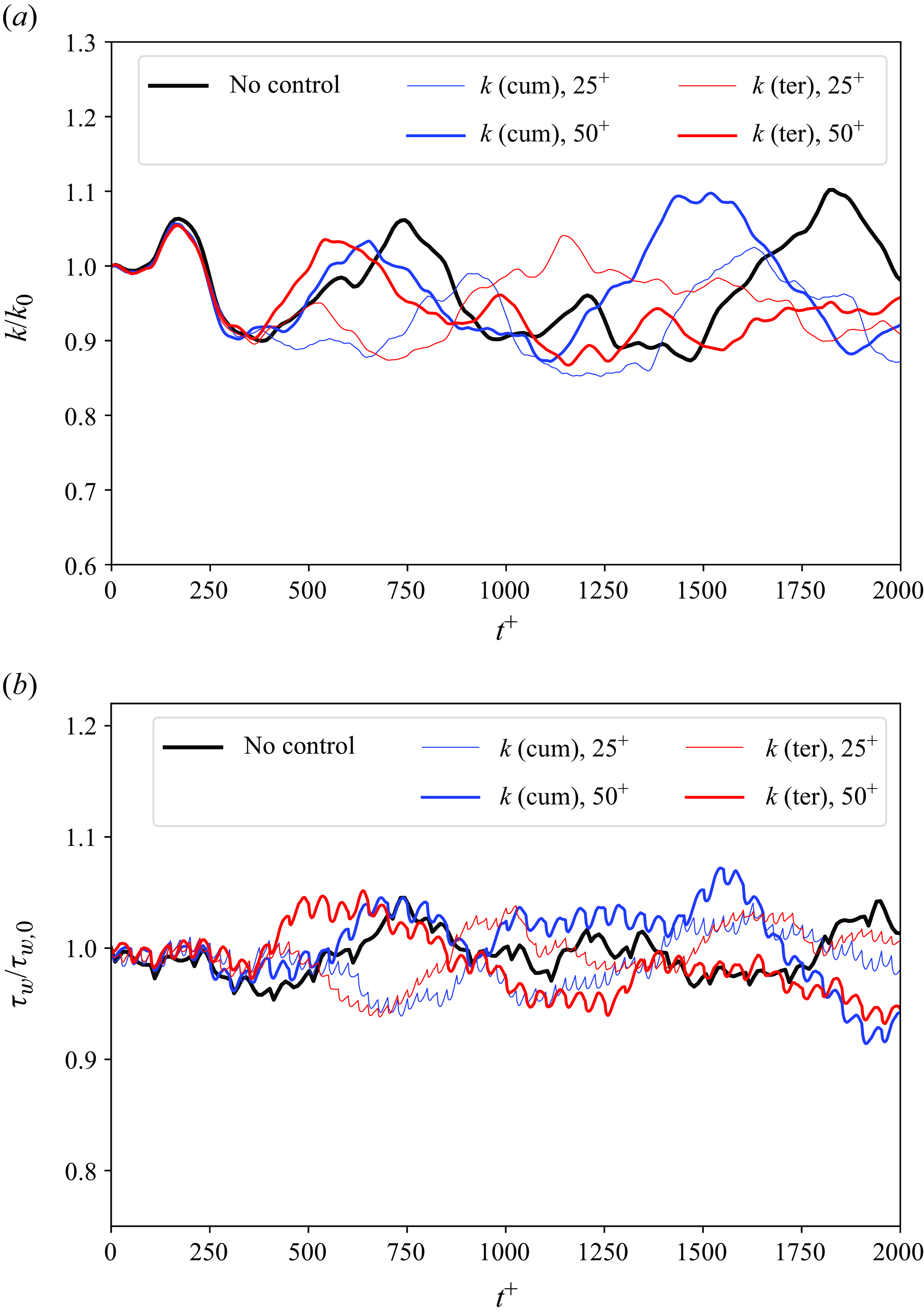
Figure 13. The history of (a) TKE $k$
and (b) wall friction
$k$
and (b) wall friction $\tau _w$
with the tunable permeable wall targeting TKE related loss function.
$\tau _w$
with the tunable permeable wall targeting TKE related loss function.
3.2.2. The characteristics of
$\beta$
distribution

The instantaneous flow fields depicted in figure 11 have demonstrated the distinctions between the $\beta$
fields in the
$\beta$
fields in the $\tau _w$
and
$\tau _w$
and $k$
control scenarios. This section delves deeper into the characteristics of the
$k$
control scenarios. This section delves deeper into the characteristics of the $\beta$
field to gain a clearer understanding of how the permeable wall adjusts to the flow field, thereby achieving drag reduction and minimising turbulence.
$\beta$
field to gain a clearer understanding of how the permeable wall adjusts to the flow field, thereby achieving drag reduction and minimising turbulence.
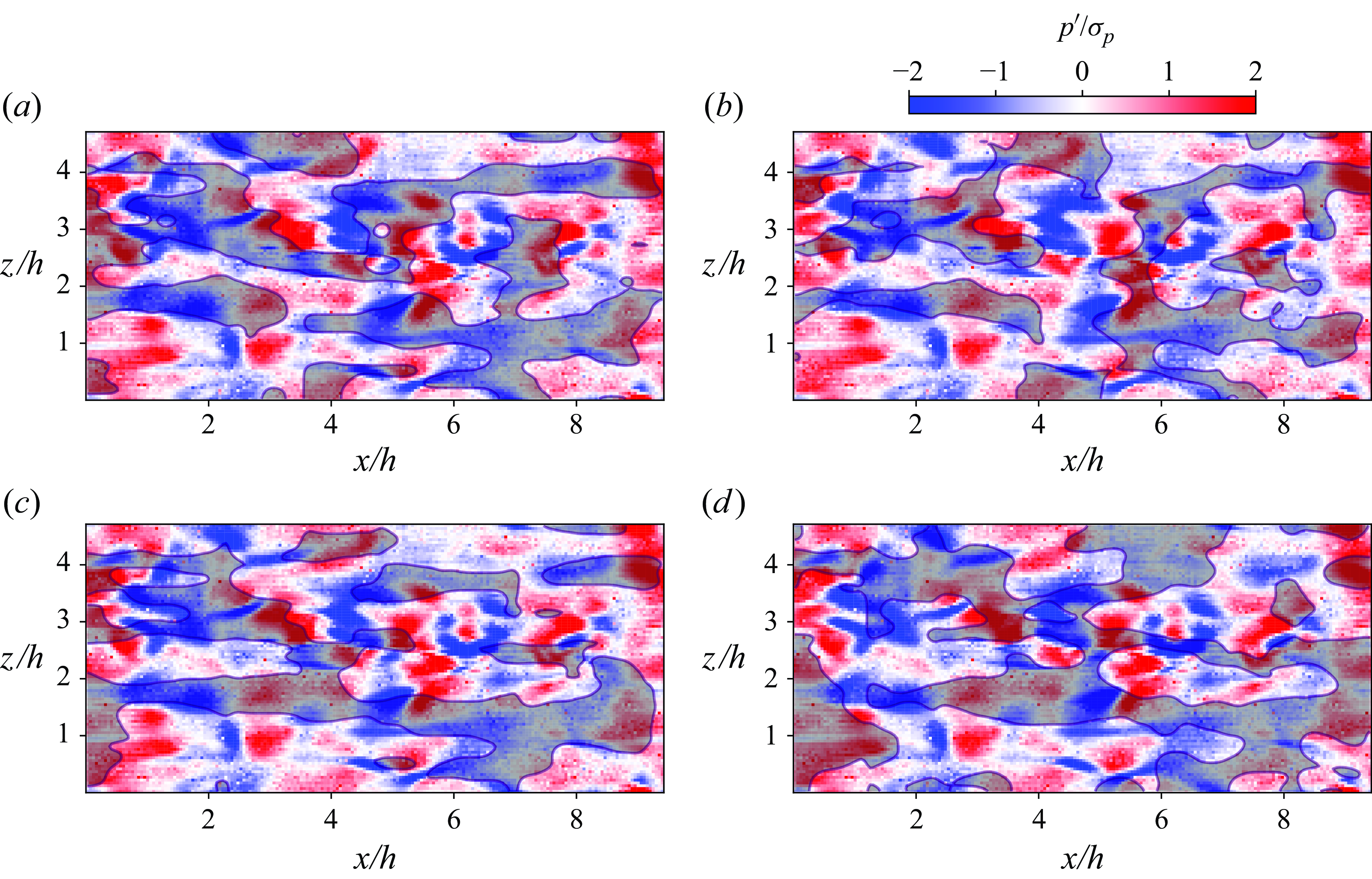
Figure 14. The $\beta$
map of the permeable wall for wall friction control with different targets and time horizons. (a) Cumulative control with
$\beta$
map of the permeable wall for wall friction control with different targets and time horizons. (a) Cumulative control with $\Delta t^+=25$
; (b) terminal control with
$\Delta t^+=25$
; (b) terminal control with $\Delta t^+=25$
; (c) cumulative control with
$\Delta t^+=25$
; (c) cumulative control with $\Delta t^+=50$
; (d) terminal control with
$\Delta t^+=50$
; (d) terminal control with $\Delta t^+=50$
. The grey patches are permeable regions with
$\Delta t^+=50$
. The grey patches are permeable regions with $\beta \geqslant 0.4$
. The colour map shows the
$\beta \geqslant 0.4$
. The colour map shows the $p'$
at buffer layer
$p'$
at buffer layer $y^+=15$
.
$y^+=15$
.
Figure 14 presents the $\beta$
fields for the
$\beta$
fields for the $\tau _w$
control scenarios, using a grey colour map. As noted in figure 11, the
$\tau _w$
control scenarios, using a grey colour map. As noted in figure 11, the $\beta$
fields predominantly exhibit two values, 0 and 0.7, which correspond to non-permeable and permeable zones. In figure 11, permeable regions where
$\beta$
fields predominantly exhibit two values, 0 and 0.7, which correspond to non-permeable and permeable zones. In figure 11, permeable regions where $\beta \geqslant 0.4$
are depicted by grey patches. Additionally, the
$\beta \geqslant 0.4$
are depicted by grey patches. Additionally, the $p'$
field from the initial state of the current episode is overlaid, allowing the inference of local
$p'$
field from the initial state of the current episode is overlaid, allowing the inference of local $v'$
at the wall.
$v'$
at the wall.
For both cumulative and terminal control scenarios, the $\beta$
map reveals a pattern that is consistent across cases. In scenarios with an extended time horizon, the permeable zones exhibit greater interconnectivity, and the primary areas remain comparable. In all instances, there is noticeable overlap between the permeable zone and the negative
$\beta$
map reveals a pattern that is consistent across cases. In scenarios with an extended time horizon, the permeable zones exhibit greater interconnectivity, and the primary areas remain comparable. In all instances, there is noticeable overlap between the permeable zone and the negative $p'$
region. This indicates that these
$p'$
region. This indicates that these $\beta$
map distributions generate a net positive wall-normal flux. The injection of additional momentum into the near-wall region can modify the velocity gradient and the characteristics of turbulence, partially elucidating the mechanism behind drag reduction. This also clarifies why the
$\beta$
map distributions generate a net positive wall-normal flux. The injection of additional momentum into the near-wall region can modify the velocity gradient and the characteristics of turbulence, partially elucidating the mechanism behind drag reduction. This also clarifies why the $\beta$
map possesses two distinct values. Strategically positioning permeable zones, especially in regions with negative
$\beta$
map possesses two distinct values. Strategically positioning permeable zones, especially in regions with negative $p'$
, to have maximum permeability supports maximal upward fluid movement, while setting non-permeable zones is crucial to entirely block any unwanted downward momentum.
$p'$
, to have maximum permeability supports maximal upward fluid movement, while setting non-permeable zones is crucial to entirely block any unwanted downward momentum.
Figure 15 illustrates the $\beta$
field in
$\beta$
field in $k$
control cases. Compared with the
$k$
control cases. Compared with the $\tau _w$
control cases in figure 14, the permeable areas in
$\tau _w$
control cases in figure 14, the permeable areas in $k$
control cases are smaller and more scattered, suggesting that the TKE control has a more stringent requirement on the wall-normal disturbances on the wall. Moreover, no obvious correlation between
$k$
control cases are smaller and more scattered, suggesting that the TKE control has a more stringent requirement on the wall-normal disturbances on the wall. Moreover, no obvious correlation between $\beta$
and
$\beta$
and $p'$
can be observed, hence, there is no net momentum flux across the wall.
$p'$
can be observed, hence, there is no net momentum flux across the wall.
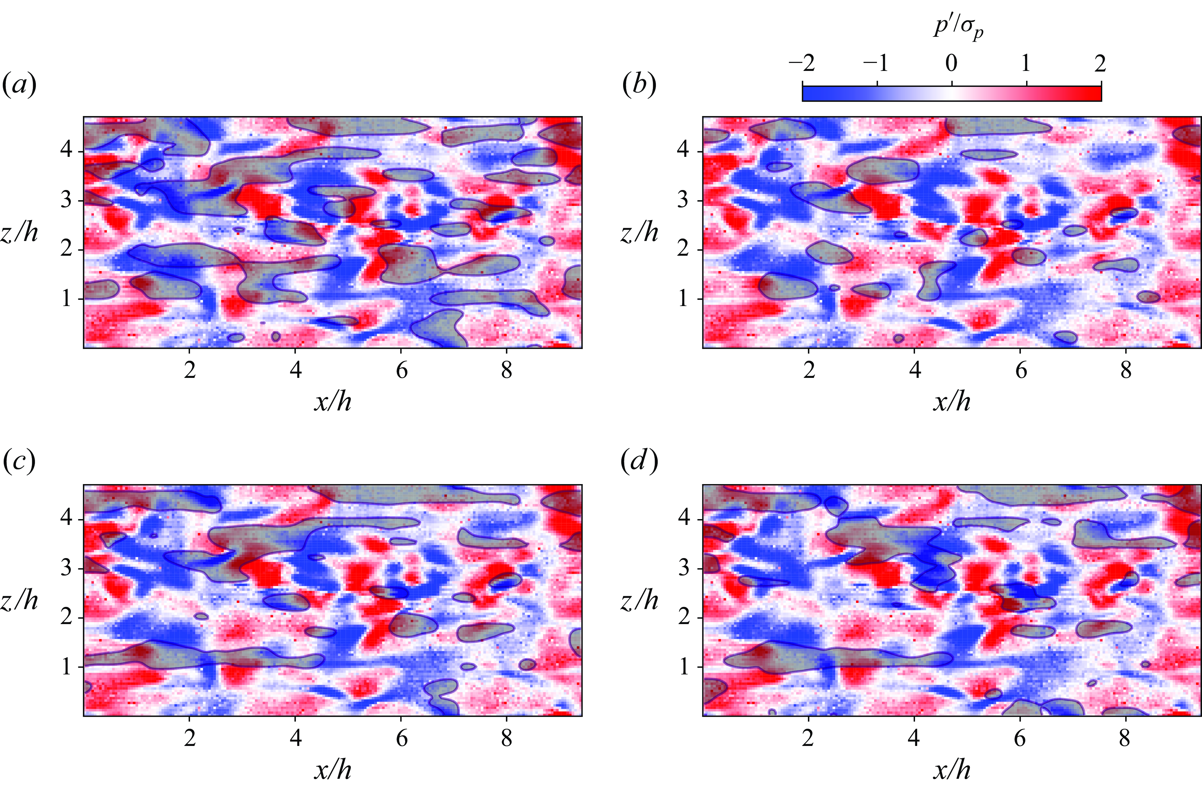
Figure 15. The $\beta$
map of the permeable wall for TKE control with different targets and time horizons. (a) Cumulative control with
$\beta$
map of the permeable wall for TKE control with different targets and time horizons. (a) Cumulative control with $\Delta t^+=25$
; (b) terminal control with
$\Delta t^+=25$
; (b) terminal control with $\Delta t^+=25$
; (c) cumulative control with
$\Delta t^+=25$
; (c) cumulative control with $\Delta t^+=50$
; (d) terminal control with
$\Delta t^+=50$
; (d) terminal control with $\Delta t^+=50$
. The other settings are the same as figure 14.
$\Delta t^+=50$
. The other settings are the same as figure 14.
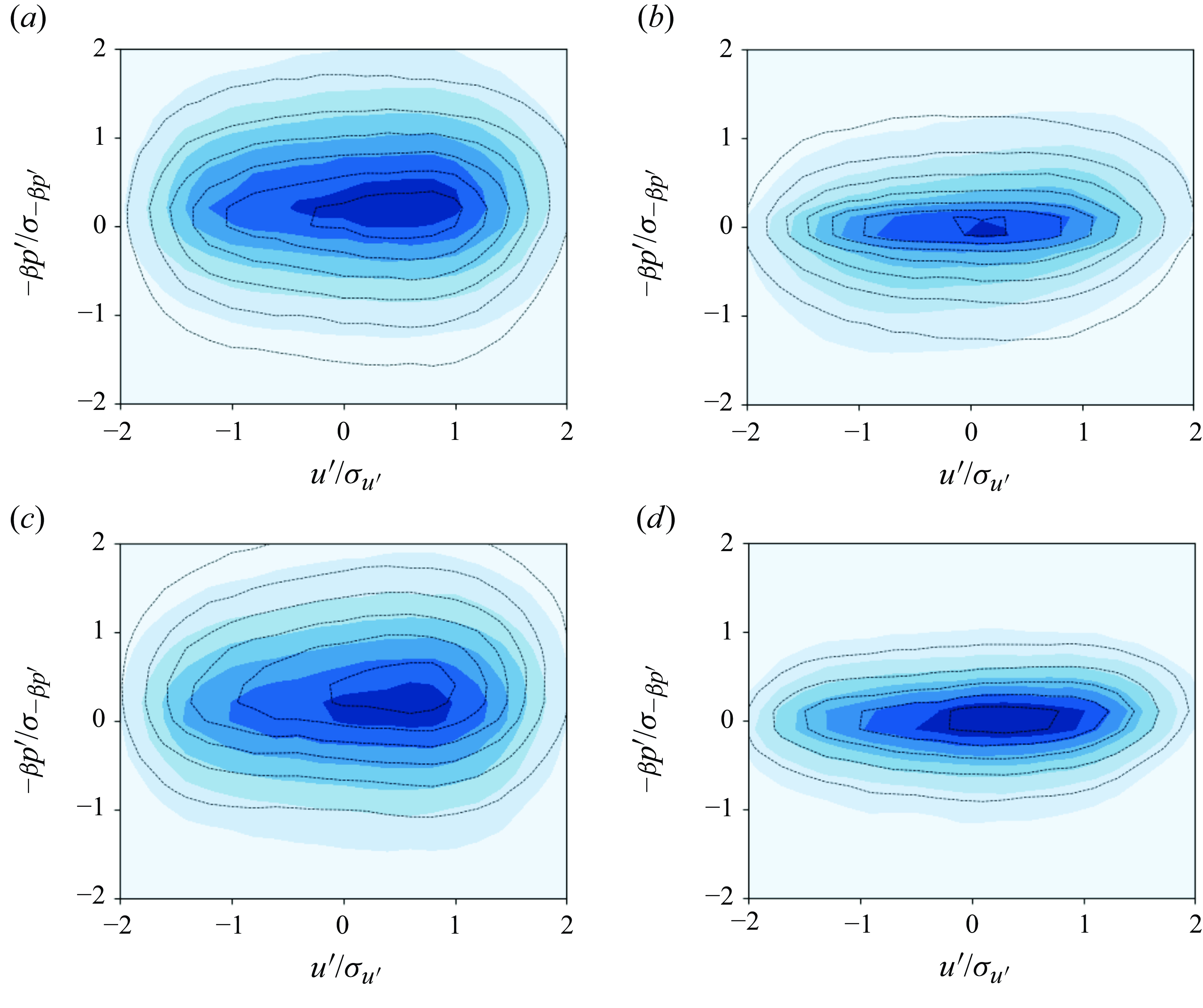
Figure 16. The joint PDF $f_{-\beta p', u'}$
between the permeable wall flux and streamwise fluctuation
$f_{-\beta p', u'}$
between the permeable wall flux and streamwise fluctuation $u'$
at
$u'$
at $y^+=15$
. (a) Cumulative control of wall friction with
$y^+=15$
. (a) Cumulative control of wall friction with $\Delta t^+=25$
; (b) cumulative control of TKE with
$\Delta t^+=25$
; (b) cumulative control of TKE with $\Delta t^+=25$
; (c) terminal control of wall friction with
$\Delta t^+=25$
; (c) terminal control of wall friction with $\Delta t^+=25$
; (d) terminal control of wall TKE with
$\Delta t^+=25$
; (d) terminal control of wall TKE with $\Delta t^+=25$
. The coloured contours show the joint PDF
$\Delta t^+=25$
. The coloured contours show the joint PDF $f_{-\beta p'_0, u^{\prime}_{0}}$
between wall flux and streamwise fluctuation
$f_{-\beta p'_0, u^{\prime}_{0}}$
between wall flux and streamwise fluctuation $u'$
at the initial time of the episodes, and the dashed isolines show the joint PDF
$u'$
at the initial time of the episodes, and the dashed isolines show the joint PDF $f_{-\beta p'_{\Delta t}, u^{\prime}_{\Delta t}}$
at the terminal time of the episodes.
$f_{-\beta p'_{\Delta t}, u^{\prime}_{\Delta t}}$
at the terminal time of the episodes.
The statistical features of the $\beta$
field are further elucidated in figure 16, which depicts the joint PDF
$\beta$
field are further elucidated in figure 16, which depicts the joint PDF $f_{-\beta p',u'}$
between the vertical velocity at the permeable wall, represented by
$f_{-\beta p',u'}$
between the vertical velocity at the permeable wall, represented by $v_w=-\beta p'$
, and the streamwise fluctuation
$v_w=-\beta p'$
, and the streamwise fluctuation $u'$
within the buffer layer (
$u'$
within the buffer layer ( $y^+=15$
). In contrast to figure 8, colour contours in this figure show the joint PDF at the start of the episodes, labelled
$y^+=15$
). In contrast to figure 8, colour contours in this figure show the joint PDF at the start of the episodes, labelled $f_{-\beta p'_0,u^{\prime}_{0}}$
, while dashed isolines illustrate the joint PDF at the episodes’ endpoint, labelled
$f_{-\beta p'_0,u^{\prime}_{0}}$
, while dashed isolines illustrate the joint PDF at the episodes’ endpoint, labelled $f_{-\beta p'_{\Delta t},u^{\prime}_{\Delta t}}$
. With cumulative
$f_{-\beta p'_{\Delta t},u^{\prime}_{\Delta t}}$
. With cumulative $\tau _w$
control (figure 16
a), the initial joint PDF
$\tau _w$
control (figure 16
a), the initial joint PDF $f_{-\beta p'_0,u^{\prime}_{0}}$
prominently biases towards the positive
$f_{-\beta p'_0,u^{\prime}_{0}}$
prominently biases towards the positive $-\beta p'$
direction, suggesting a positive wall-normal flux. At the terminal time, a smaller bias is noted in
$-\beta p'$
direction, suggesting a positive wall-normal flux. At the terminal time, a smaller bias is noted in $f_{-\beta p'_{\Delta t},u^{\prime}_{\Delta t}}$
. Conversely, under terminal
$f_{-\beta p'_{\Delta t},u^{\prime}_{\Delta t}}$
. Conversely, under terminal $\tau _w$
control (figure 16
c), the terminal joint PDF
$\tau _w$
control (figure 16
c), the terminal joint PDF $f_{-\beta p'_{\Delta t},u^{\prime}_{\Delta t}}$
exhibits a more pronounced bias to the positive
$f_{-\beta p'_{\Delta t},u^{\prime}_{\Delta t}}$
exhibits a more pronounced bias to the positive $-\beta p'$
than the initial joint PDF
$-\beta p'$
than the initial joint PDF $f_{-\beta p'_0,u^{\prime}_{0}}$
, implying that most of the wall-normal flux occurs at the episodes’ conclusion. For both cumulative and terminal
$f_{-\beta p'_0,u^{\prime}_{0}}$
, implying that most of the wall-normal flux occurs at the episodes’ conclusion. For both cumulative and terminal $\tau _w$
control scenarios, the
$\tau _w$
control scenarios, the $f_{-\beta p',u'}$
displays symmetry around its horizontal centreline, indicating no significant correlation between these variables.
$f_{-\beta p',u'}$
displays symmetry around its horizontal centreline, indicating no significant correlation between these variables.
In the cumulative $k$
control (figure 16
b) , the wall-normal flux
$k$
control (figure 16
b) , the wall-normal flux $-\beta p'$
poses a weak positive correlation with
$-\beta p'$
poses a weak positive correlation with $u_0'$
with the shape of
$u_0'$
with the shape of $f_{-\beta p'_0,u^{\prime}_{0}}$
skewing towards the first and third quadrants. Such positive correlation is not seen in the terminal joint PDF
$f_{-\beta p'_0,u^{\prime}_{0}}$
skewing towards the first and third quadrants. Such positive correlation is not seen in the terminal joint PDF $f_{-\beta p'_{\Delta t},u^{\prime}_{\Delta t}}$
. A weak positive correlation between
$f_{-\beta p'_{\Delta t},u^{\prime}_{\Delta t}}$
. A weak positive correlation between $-\beta p'$
and
$-\beta p'$
and $u'$
is also observed in the joint PDFs in the terminal
$u'$
is also observed in the joint PDFs in the terminal $k$
control case (figure 16
d).
$k$
control case (figure 16
d).
The joint PDFs in figure 16 confirm our observation in the instantaneous $\beta$
fields in figures 14 and 15. For wall friction control, the permeable wall adopted a completely different strategy than the opposition control, that is, exploiting the tunable permeability to inject net upward momentum in the near-wall region in order to alter the shear at the wall. The TKE control, however, shares the same mechanism with opposition control. In this case, wall-normal velocity induced by the permeable region is positively correlated to the
$\beta$
fields in figures 14 and 15. For wall friction control, the permeable wall adopted a completely different strategy than the opposition control, that is, exploiting the tunable permeability to inject net upward momentum in the near-wall region in order to alter the shear at the wall. The TKE control, however, shares the same mechanism with opposition control. In this case, wall-normal velocity induced by the permeable region is positively correlated to the $u'$
near the wall, hence cancelling the local Reynolds stress, which eventually leads to drag reduction.
$u'$
near the wall, hence cancelling the local Reynolds stress, which eventually leads to drag reduction.
3.2.3. The mean statistics and wall friction decomposition
To elaborate on how drag is reduced using a permeable wall, we analyse the flow field statistics in this section. Table 2 provides a comparison of wall friction between the permeable wall channel and the smooth wall channel (refer to table 1). It is evident that only the cumulative $\tau _w$
control with
$\tau _w$
control with $\Delta t^+=25$
achieves a 15 % reduction in drag, while the effectiveness of other methods remains under 8 %.
$\Delta t^+=25$
achieves a 15 % reduction in drag, while the effectiveness of other methods remains under 8 %.
Table 2. The relative wall friction change in permeable wall cases.
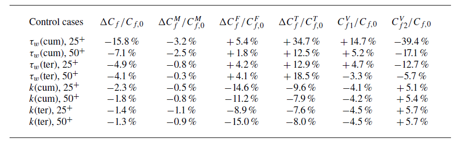
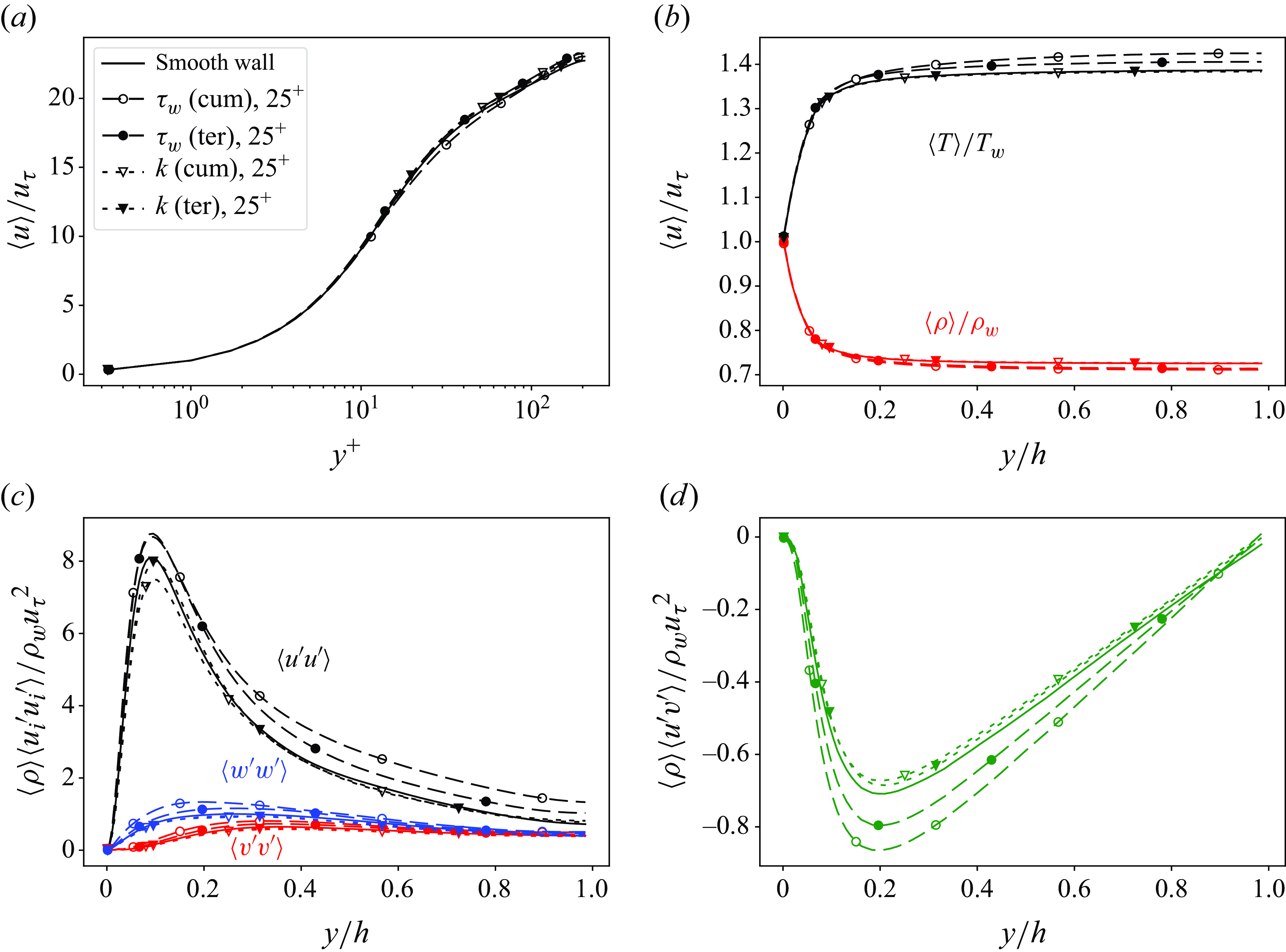
Figure 17. Mean statistics of permeable wall cases compared with the smooth wall channel. (a) Mean streamwise velocity $\langle u\rangle$
; (b) mean temperature
$\langle u\rangle$
; (b) mean temperature $\langle T\rangle$
and mean density
$\langle T\rangle$
and mean density $\langle \rho \rangle$
; (c) turbulent intensity
$\langle \rho \rangle$
; (c) turbulent intensity $\langle u_i'u_i'\rangle$
; (d) Reynolds stress
$\langle u_i'u_i'\rangle$
; (d) Reynolds stress $\langle u'v'\rangle$
.
$\langle u'v'\rangle$
.
Figure 17 presents the average statistics for four selected permeable wall cases. We chose the cases with a shorter time horizon $\Delta t^+=25$
, as they generally outperform the long time horizon ones. The mean streamwise velocity profiles (figure 17
a) remain largely unchanged due to the low drag reduction rate. In the
$\Delta t^+=25$
, as they generally outperform the long time horizon ones. The mean streamwise velocity profiles (figure 17
a) remain largely unchanged due to the low drag reduction rate. In the $\tau _w$
control scenarios, the temperature at the channel’s centre (figure 17
b) shows a slight increase. This is attributed to a rise in turbulence intensity and Reynolds stress (figure 17
c,d), leading to more heat being dissipated into the channel and mildly reducing
$\tau _w$
control scenarios, the temperature at the channel’s centre (figure 17
b) shows a slight increase. This is attributed to a rise in turbulence intensity and Reynolds stress (figure 17
c,d), leading to more heat being dissipated into the channel and mildly reducing $\rho$
. Conversely, in the
$\rho$
. Conversely, in the $k$
control scenarios, both turbulence intensity and Reynolds stress exhibit a slight decrease.
$k$
control scenarios, both turbulence intensity and Reynolds stress exhibit a slight decrease.
To further understand the source of drag on permeable wall cases, we inspect the decomposition of wall friction. Note that for the permeable wall condition, the zero-net-flux condition does not hold anymore, therefore, we have to rederive the RD identity to include the additional terms generated by this. Here we show the RD identity for the compressible channel with the permeable wall:
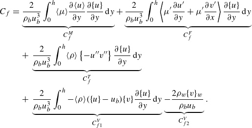 \begin{eqnarray} C_f &=& \underbrace {\frac {2}{\rho _b u_b^3} \int _0^h\langle \mu \rangle \frac {\partial \langle u\rangle }{\partial y} \frac {\partial \{u\}}{\partial y} \textrm {d} y}_{C_{f}^M}+\underbrace {\frac {2}{\rho _b u_b^3} \int _0^h\left \langle \mu ^{\prime } \frac {\partial u^{\prime }}{\partial y}+\mu ^{\prime } \frac {\partial v^{\prime }}{\partial x}\right \rangle \frac {\partial \{u\}}{\partial y} \textrm {d} y}_{C_{f}^F}\nonumber\\&& + \underbrace {\frac {2}{\rho _b u_b^3} \int _0^h\langle \rho \rangle \left \{-u^{\prime \prime } v^{\prime \prime }\right \} \frac {\partial \{u\}}{\partial y} \textrm {d} y}_{C_{f }^T}\\&& + \underbrace {\frac {2}{\rho _b u_b^3} \int _0^h-\langle \rho \rangle (\{u\}-u_b)\{v\}\frac {\partial \{u\} }{\partial y} \textrm {d} y}_{C_{f1}^V}\underbrace {-\frac {2\rho _w \{ v\}_w}{\rho _b u_b}}_{C_{f2}^V}. \nonumber \end{eqnarray}
Comparing to the original RD identity equation (3.1), two additional terms $C_{f1}^V$
and
$C_{f1}^V$
and $C_{f2}^V$
emerged, representing the effect of mean convection in the wall-normal direction. The first term
$C_{f2}^V$
emerged, representing the effect of mean convection in the wall-normal direction. The first term $C_{f1}^V$
is the gain of mean streamwise kinetic energy in the absolute frame. The term
$C_{f1}^V$
is the gain of mean streamwise kinetic energy in the absolute frame. The term $C_{f2}^V$
represents the effect of fluid injection at the permeable wall, showing that a positive
$C_{f2}^V$
represents the effect of fluid injection at the permeable wall, showing that a positive $\{v\}$
flux at the wall would directly reduce the mean friction coefficient. The full derivation of (3.2) is in Appendix D. For the permeable wall cases, the residual error for the extended RD identity is confined within
$\{v\}$
flux at the wall would directly reduce the mean friction coefficient. The full derivation of (3.2) is in Appendix D. For the permeable wall cases, the residual error for the extended RD identity is confined within $\pm 3.5\,\%$
, which is slightly larger compared with the opposition control cases with the initial RD identity. This could be attributed to the limited sample time and the continuous momentum injection at the wall, which can violate the assumption of temporal homogeneity (see (3.2)). However, the decomposition is still fairly reliable and may provide insight into wall friction over permeable walls.
$\pm 3.5\,\%$
, which is slightly larger compared with the opposition control cases with the initial RD identity. This could be attributed to the limited sample time and the continuous momentum injection at the wall, which can violate the assumption of temporal homogeneity (see (3.2)). However, the decomposition is still fairly reliable and may provide insight into wall friction over permeable walls.
Table 2 lists the relative change in the components of RD identity for permeable wall cases. Note that for $C_{f1}^V$
and
$C_{f1}^V$
and $C_{f2}^V$
, the relative change is compared with the total friction. In the
$C_{f2}^V$
, the relative change is compared with the total friction. In the $\tau _w$
control scenarios, the main contributor to the reduction of drag is the wall flux term
$\tau _w$
control scenarios, the main contributor to the reduction of drag is the wall flux term $C_{f2}^V$
, which aligns with previous observations of a net positive
$C_{f2}^V$
, which aligns with previous observations of a net positive $-\beta p'$
in figure 16(a,c). However, the drag reduction attributed to wall flux is significantly counteracted by the increase in the kinetic energy of the turbulence
$-\beta p'$
in figure 16(a,c). However, the drag reduction attributed to wall flux is significantly counteracted by the increase in the kinetic energy of the turbulence $C_f^T$
and the kinetic energy of mean convection
$C_f^T$
and the kinetic energy of mean convection $C_{f1}^V$
. Despite this, the cumulative
$C_{f1}^V$
. Despite this, the cumulative $\tau _w$
control with
$\tau _w$
control with $t^+=25$
, with a maximum induced upward flux through the permeable wall, produces the highest drag reduction rate up to 15.8 %.
$t^+=25$
, with a maximum induced upward flux through the permeable wall, produces the highest drag reduction rate up to 15.8 %.
In all the TKE control cases, a slightly positive $C_{f2}^V$
is observed, which suggests a weak downward net flux at the wall. This minor magnitude is not clearly depicted in figure 16(b,d). The presence of downward flux at the wall decreases the kinetic energy of both mean convection and turbulence, which results in a reduction in
$C_{f2}^V$
is observed, which suggests a weak downward net flux at the wall. This minor magnitude is not clearly depicted in figure 16(b,d). The presence of downward flux at the wall decreases the kinetic energy of both mean convection and turbulence, which results in a reduction in $C_{f1}^V$
and
$C_{f1}^V$
and $C_{f}^T$
. Additionally, the mean shear in the near-wall region is altered, leading to a diminished
$C_{f}^T$
. Additionally, the mean shear in the near-wall region is altered, leading to a diminished $C_f^M$
. Despite all these favourable changes to the flow, the overall drag reduction remains relatively minor compared with the
$C_f^M$
. Despite all these favourable changes to the flow, the overall drag reduction remains relatively minor compared with the $\tau _w$
control cases.
$\tau _w$
control cases.
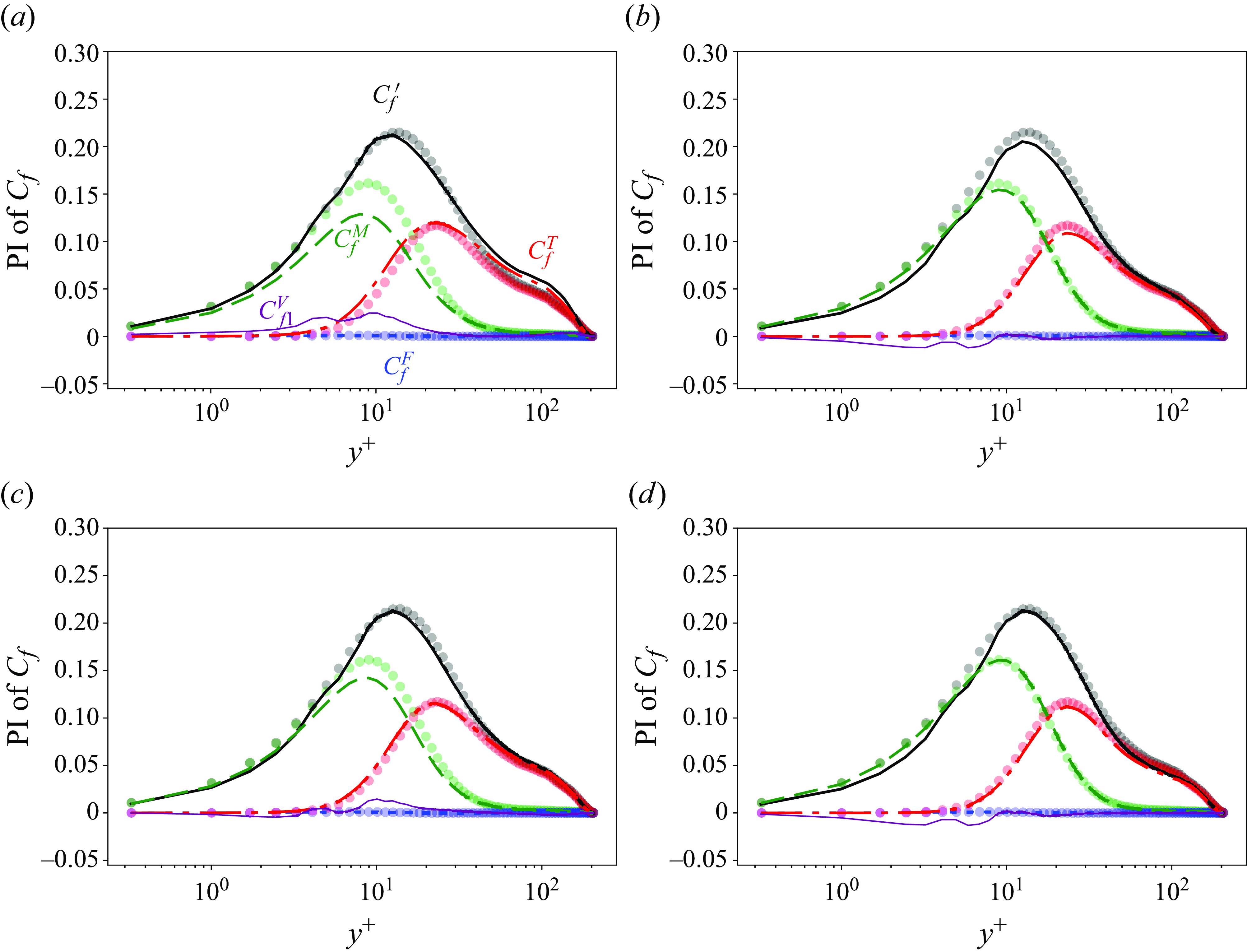
Figure 18. Premultiplied integrands (PI) of RD identity as a function of $y^+$
for tunable permeable wall cases. Here
$y^+$
for tunable permeable wall cases. Here $C_f^M$
,
$C_f^M$
, $C_f^F$
,
$C_f^F$
, $C_f^T$
and
$C_f^T$
and $C_{f1}^V$
are denoted by dashed lines, dotted lines, dash-dotted lines and thin solid lines, respectively. The sum of all the integrands
$C_{f1}^V$
are denoted by dashed lines, dotted lines, dash-dotted lines and thin solid lines, respectively. The sum of all the integrands $C_{f}^{\prime}$
are denoted by thick solid lines, where the contribution of
$C_{f}^{\prime}$
are denoted by thick solid lines, where the contribution of $C_{f2}^V$
is not included. The PI of the smooth wall channel is superimposed with circles of corresponding colours. (a) Cumulative
$C_{f2}^V$
is not included. The PI of the smooth wall channel is superimposed with circles of corresponding colours. (a) Cumulative $\tau _w$
control,
$\tau _w$
control, $\Delta t^+=25$
; (b) cumulative
$\Delta t^+=25$
; (b) cumulative $k$
control,
$k$
control, $\Delta t^+=25$
; (c) terminal
$\Delta t^+=25$
; (c) terminal $\tau _w$
control,
$\tau _w$
control, $\Delta t^+=25$
; (d) terminal
$\Delta t^+=25$
; (d) terminal $k$
control,
$k$
control, $\Delta t^+=25$
.
$\Delta t^+=25$
.
The premultiplied integrands of RD identity for the four typical cases in figure 17 is shown in figure 18. Note that $C_{f2}^V$
is not in the form of integration and is not shown in figure 18. For the
$C_{f2}^V$
is not in the form of integration and is not shown in figure 18. For the $\tau _w$
control cases (figure 18
a,c), the mean shear term close to the wall is reduced. Meanwhile, the turbulent production term
$\tau _w$
control cases (figure 18
a,c), the mean shear term close to the wall is reduced. Meanwhile, the turbulent production term $C_f^T$
is enhanced. The net wall flux induces the vertical mean convection velocity, introduces extra
$C_f^T$
is enhanced. The net wall flux induces the vertical mean convection velocity, introduces extra $C_{f1}^V$
in the near-wall area. This observation is consistent with our previous findings that the permeable wall in the
$C_{f1}^V$
in the near-wall area. This observation is consistent with our previous findings that the permeable wall in the $\tau _w$
control cases induces upward flux at the wall, altering the near-wall shear stress and mean convect in the channel.
$\tau _w$
control cases induces upward flux at the wall, altering the near-wall shear stress and mean convect in the channel.
As for the $k$
control cases (figure 18
b,d), both
$k$
control cases (figure 18
b,d), both $C_f^T$
is reduced slightly, indicating the flux induced by permeable present an ‘opposition control’ effect on the turbulence field. The
$C_f^T$
is reduced slightly, indicating the flux induced by permeable present an ‘opposition control’ effect on the turbulence field. The $C_f^M$
is also slightly reduced. The downward wall flux also produces favourable
$C_f^M$
is also slightly reduced. The downward wall flux also produces favourable $C_{f1}^V$
. However, these reduction sources are countered by
$C_{f1}^V$
. However, these reduction sources are countered by $C_{f2}^V$
, resulting in a marginal drag reduction result.
$C_{f2}^V$
, resulting in a marginal drag reduction result.
It appears that the optimisation process effectively identified a ‘shortcut’ for the $\tau _w$
control cases, which is indirectly injecting momentum into the boundary layer by adjusting the distribution of permeability. This control mechanism is consistent with the mass bleed control strategy (Lee & Kim Reference Lee and Kim2006), which alters the flow behaviour through a managed mass flow to the surface. Furthermore, we tested that the optimisation results for the cumulative
$\tau _w$
control cases, which is indirectly injecting momentum into the boundary layer by adjusting the distribution of permeability. This control mechanism is consistent with the mass bleed control strategy (Lee & Kim Reference Lee and Kim2006), which alters the flow behaviour through a managed mass flow to the surface. Furthermore, we tested that the optimisation results for the cumulative $\tau _w$
control with
$\tau _w$
control with $\Delta t^+=25$
show insensitivity to the initial
$\Delta t^+=25$
show insensitivity to the initial $\beta$
(see Appendix C). The alignment of optimised control mechanisms with established methods further validates the efficiency of the current optimisation framework.
$\beta$
(see Appendix C). The alignment of optimised control mechanisms with established methods further validates the efficiency of the current optimisation framework.
Despite the fact that the drag reduction performance of the tunable permeable wall is far below opposition control, we demonstrate that a permeable wall with only a vertical permeability component can also achieve drag reduction when its local permeability is adjustable over time. It is also important to note that the adjustable permeable wall used in this study is not entirely a passive control method. Modulation of the wall permeability will undoubtedly consume energy. Bearing this in mind, cases with shorter episodes benefit from a higher energy input. This partly clarifies why the $t^+=25$
cases are generally more effective.
$t^+=25$
cases are generally more effective.
4. Conclusive remarks
In this study we have designed an AD-based optimisation framework based on the fully differentiable solver JAX-Fluids for flow control in compressible turbulent channel flows. By developing a fully differentiable boundary condition, the exact gradients with respect to boundary control parameters are computed, enabling efficient optimisation of flow control strategies.
The study investigated two primary flow control strategies: opposition control and tunable permeable walls. We adopted the receding-horizon predictive control process, which consists of a series of ‘episodes’. In each optimisation episode there were around $192\times 96\times 2\approx 4\times 10^4$
control variables and
$192\times 96\times 2\approx 4\times 10^4$
control variables and $192\times 96\times 128\times 1200\approx 3\times 10^{9}$
state variables. We explored the two control strategies under different optimisation targets, specifically wall friction
$192\times 96\times 128\times 1200\approx 3\times 10^{9}$
state variables. We explored the two control strategies under different optimisation targets, specifically wall friction $\tau _w$
and TKE, across varying time horizons. Opposition control strategies targeting TKE consistently outperform those directly minimising
$\tau _w$
and TKE, across varying time horizons. Opposition control strategies targeting TKE consistently outperform those directly minimising $\tau _w$
in terms of stability and effectiveness. Specifically, terminal TKE control with
$\tau _w$
in terms of stability and effectiveness. Specifically, terminal TKE control with $\Delta t^+=50$
manages to reduce drag by approximately 20 % by diminishing turbulence intensity across the entire channel domain.
$\Delta t^+=50$
manages to reduce drag by approximately 20 % by diminishing turbulence intensity across the entire channel domain.
In contrast, opposition control directly targeting $\tau _w$
appears to be less effective. Although this strategy initially showed a promising result in the initial phase of the control, it suffered from instability over longer time scales, particularly with terminal
$\tau _w$
appears to be less effective. Although this strategy initially showed a promising result in the initial phase of the control, it suffered from instability over longer time scales, particularly with terminal $\tau _w$
controls. This instability comes from the tendency of the
$\tau _w$
controls. This instability comes from the tendency of the $\tau _w$
control to push energetic turbulence structures away from the wall, leading to an increase in turbulent fluctuations in the outer flow region. The resulting redistribution of turbulence often led to an overall increase in Reynolds stresses, undermining the effectiveness of friction reduction. These findings highlight the importance of selecting loss functions that include information from the entire flow field to ensure stable and effective control outcomes.
$\tau _w$
control to push energetic turbulence structures away from the wall, leading to an increase in turbulent fluctuations in the outer flow region. The resulting redistribution of turbulence often led to an overall increase in Reynolds stresses, undermining the effectiveness of friction reduction. These findings highlight the importance of selecting loss functions that include information from the entire flow field to ensure stable and effective control outcomes.
We also explored the potential of using a tunable permeable wall as a quasi-passive control mechanism. Unlike active methods such as opposition control, the tunable permeable wall does not directly inject or remove mass directly from the flow. Instead, it modulates the flow dynamics through spatial variations in wall permeability. The performance of this strategy appears to be quite stable, even with terminal $\tau _w$
control cases. This stability is attributed to its naturally constrained wall-normal flux, which prevents excessive disturbances and ensures a gradual and mild control input.
$\tau _w$
control cases. This stability is attributed to its naturally constrained wall-normal flux, which prevents excessive disturbances and ensures a gradual and mild control input.
The permeable wall demonstrated the ability to achieve up to 15 % drag reduction using cumulative $ \tau _w$
as loss functions. This is achieved by consistently inducing upward flux by adjusting the local permeability, which adds momentum into the near-wall region. It is proven with wall friction decomposition that this upward momentum contributes directly to drag reduction. However, the effectiveness of the permeable wall in reducing TKE was notably limited compared with the opposition control. This is likely due to its inherent limitations in dynamically adjusting the flow field, as the boundary condition only allows controlled leakage rather than active momentum injection. Nonetheless, stable reduction of drag using an adjustable permeable wall has been seldom investigated, and it presents a novel opportunity for the application of porous materials in industrial settings.
$ \tau _w$
as loss functions. This is achieved by consistently inducing upward flux by adjusting the local permeability, which adds momentum into the near-wall region. It is proven with wall friction decomposition that this upward momentum contributes directly to drag reduction. However, the effectiveness of the permeable wall in reducing TKE was notably limited compared with the opposition control. This is likely due to its inherent limitations in dynamically adjusting the flow field, as the boundary condition only allows controlled leakage rather than active momentum injection. Nonetheless, stable reduction of drag using an adjustable permeable wall has been seldom investigated, and it presents a novel opportunity for the application of porous materials in industrial settings.
It should be noted that the control methods employed in this study rely on ideal assumptions. For example, the switch time for the control velocity $\phi$
and the porosity coefficient
$\phi$
and the porosity coefficient $\beta$
between episodes is considered zero. In reality, flow rate changes or material porosity adjustments require reaction time based on actuator performance or material properties. Furthermore, the energy used to generate and maintain
$\beta$
between episodes is considered zero. In reality, flow rate changes or material porosity adjustments require reaction time based on actuator performance or material properties. Furthermore, the energy used to generate and maintain $\phi$
and
$\phi$
and $\beta$
, including mechanical and electrical energy by actuators and control systems, is ignored. To create control strategies suitable for real-world scenarios, a more precise control model and refined loss function taking these aspects into account are necessary.
$\beta$
, including mechanical and electrical energy by actuators and control systems, is ignored. To create control strategies suitable for real-world scenarios, a more precise control model and refined loss function taking these aspects into account are necessary.
The integration of AD into fluid dynamics simulations offers a powerful tool for optimising flow control with high dimensionality and nonlinearity. The AD-based approach significantly reduces the complexity associated with traditional adjoint methods, making it more accessible for a wider range of flow control and optimisation applications. The findings of this study suggest several avenues for future research. First, extending the optimisation framework to higher Mach number flows could provide valuable insights into the control of supersonic and hypersonic boundary layers, where thermal and aerodynamic effects are more pronounced. Moreover, the potential to integrate AD-based optimisation with ML techniques, such as RL, could enable adaptive control strategies that dynamically adjust to changing flow conditions in real time.
Supplementary movies
Supplementary movies are available at https://doi.org/10.1017/jfm.2025.304.
Acknowledgements
This work is supported by the Fundamental Research Funds for the Central Universities (China). All authors gratefully acknowledge the access to the high performance computing facility Hawk-AI at HLRS, Stuttgart. XC appreciates the funding support from Royal Society (RG\R1\251236). We would like to express our gratitude for the valuable discussions and support provided by Professor Nikolaus Adams, Deniz Bezgin and Aaron Buhendwa from TU München.
Declaration of interests
The authors report no conflict of interest.
Appendix A. Validation of DNS channel flow
Figure 19 shows a comparison of the current DNS results with those of Yao & Hussain (2020) for validation of basic turbulent flow statistics. Yao’s DNS had a resolution of 512 $\times$
129
$\times$
129 $\times$
256, with a domain size of
$\times$
256, with a domain size of $6\pi \times 2 \times 2\pi$
, which is larger in the streamwise and spanwise directions, and features a higher resolution than the current DNS set-up. Despite these differences, figure 19(a) shows that the mean streamwise velocity profile
$6\pi \times 2 \times 2\pi$
, which is larger in the streamwise and spanwise directions, and features a higher resolution than the current DNS set-up. Despite these differences, figure 19(a) shows that the mean streamwise velocity profile $ \langle u \rangle / u_{\tau }$
, plotted against the wall-normal coordinate
$ \langle u \rangle / u_{\tau }$
, plotted against the wall-normal coordinate $ y^+$
, demonstrates excellent agreement between the current DNS (solid black line) and the reference data from Yao & Hussain (2020) (grey circles). In figure 19(b) the temperature
$ y^+$
, demonstrates excellent agreement between the current DNS (solid black line) and the reference data from Yao & Hussain (2020) (grey circles). In figure 19(b) the temperature $ \langle T \rangle / T_w$
and density
$ \langle T \rangle / T_w$
and density $ \langle \rho \rangle / \rho _w$
profiles are shown as functions of the normalised wall-normal distance
$ \langle \rho \rangle / \rho _w$
profiles are shown as functions of the normalised wall-normal distance $ y/h$
. The current DNS captures the near-wall temperature peak and the density decay towards the centreline accurately, aligning well with the reference data. Figure 19(c) compares the Reynolds stress components
$ y/h$
. The current DNS captures the near-wall temperature peak and the density decay towards the centreline accurately, aligning well with the reference data. Figure 19(c) compares the Reynolds stress components $\langle u^{\prime}_{i}u^{\prime}_{j} \rangle$
between the current DNS (solid lines) and the reference DNS (circle markers). Strong agreement is observed across all components, demonstrating that the current DNS captures the key turbulent stress distributions despite the differences in resolution and domain size. This comparison confirms the reliability of the current DNS in reproducing the essential turbulent flow features and stress profiles.
$\langle u^{\prime}_{i}u^{\prime}_{j} \rangle$
between the current DNS (solid lines) and the reference DNS (circle markers). Strong agreement is observed across all components, demonstrating that the current DNS captures the key turbulent stress distributions despite the differences in resolution and domain size. This comparison confirms the reliability of the current DNS in reproducing the essential turbulent flow features and stress profiles.
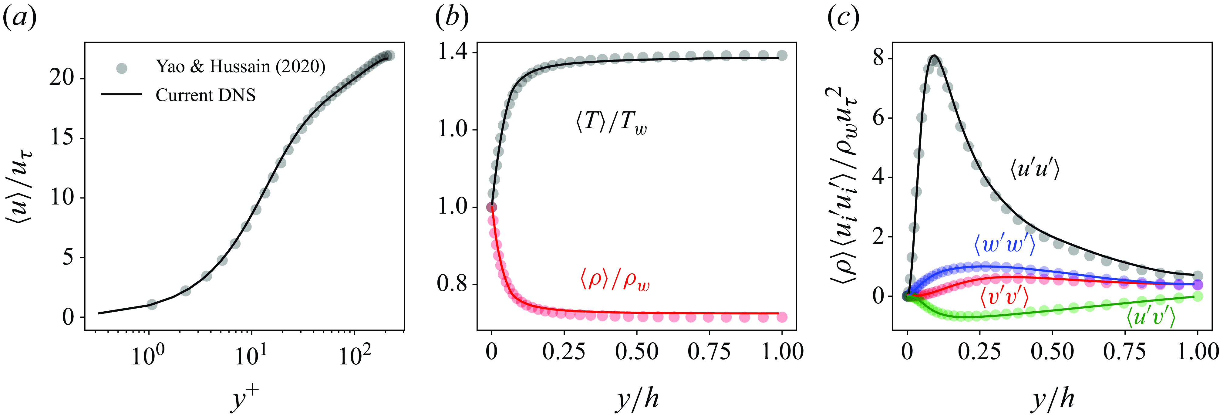
Figure 19. Comparison of mean statistics between the current DNS and Yao & Hussain (Reference Yao and Hussain2020). (a) Mean streamwise velocity $\langle u\rangle$
;(b) mean temperature
$\langle u\rangle$
;(b) mean temperature $\langle T\rangle$
and mean density
$\langle T\rangle$
and mean density $\langle \rho \rangle$
; (c) turbulent intensity
$\langle \rho \rangle$
; (c) turbulent intensity $\langle u_i'u_i'\rangle$
and Reynolds stress
$\langle u_i'u_i'\rangle$
and Reynolds stress $\langle u'v'\rangle$
.
$\langle u'v'\rangle$
.
Appendix B. Validation of AD with finite difference
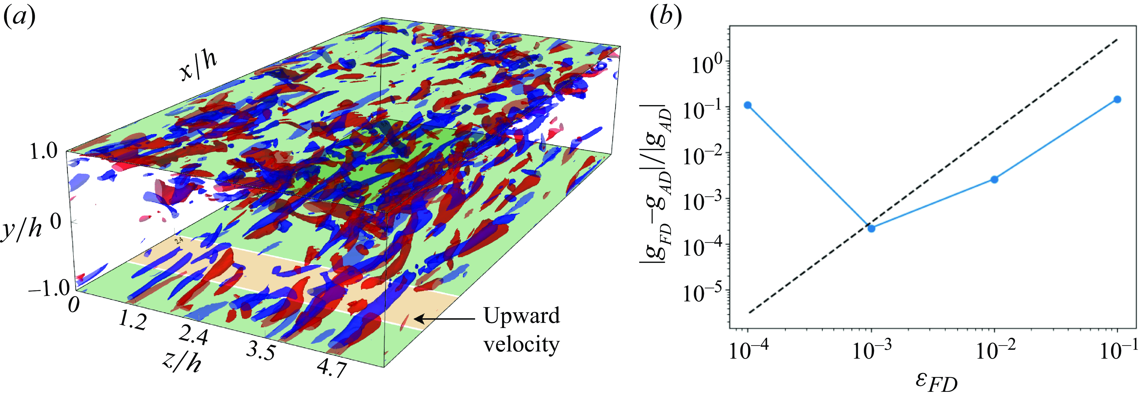
Figure 20. (a) Opposition control set-up for AD validation. The green regions near the upper and lower walls represent areas where the control amplitude is set to zero, while the orange regions denote areas with a uniform control amplitude $\phi$
. (b) Convergence of FD gradients towards AD gradients.. The blue line represents the relative error between FD and AD gradients as a function of the step size. The dashed line indicates second-order convergence.
$\phi$
. (b) Convergence of FD gradients towards AD gradients.. The blue line represents the relative error between FD and AD gradients as a function of the step size. The dashed line indicates second-order convergence.
We validate AD using a FD method in the context of opposition control. Figure 20(a) shows the case set-up. The green areas in the upper and lower walls represent regions where the opposition control amplitude is set to zero. The orange regions denote areas where the control amplitude is assigned a finite uniform value $\alpha$
. We evaluated the sensitivity of the cumulative TKE over a horizon of
$\alpha$
. We evaluated the sensitivity of the cumulative TKE over a horizon of $\Delta t^+ = 50$
with respect to the amplitude
$\Delta t^+ = 50$
with respect to the amplitude $\alpha$
when
$\alpha$
when $\alpha =0$
using both AD and FD methods.
$\alpha =0$
using both AD and FD methods.
Note that instead of computing the gradient at a point on the control surface, we compute the gradient over an area of uniform control input. This lies in the nature of the methods being compared. While AD can compute gradients accurately even with a control input applied at a single point, FD methods struggle with this due to round-off errors. When using a very small control input like a single point, the changes in the output can be too subtle, causing the finite difference to become unreliable because it cannot distinguish these small variations amidst numerical noise.
Figure 20(b) displays the comparison between the derivatives computed through AD and those obtained using the FD approach. Specifically, we use a second-order central difference scheme where the amplitude is incremented by $\epsilon _{\textit{FD}}$
, leading to a derivative estimate through
$\epsilon _{\textit{FD}}$
, leading to a derivative estimate through
 \begin{equation} g_{\textit{FD}}=(k|_{\alpha = \varepsilon _{\textit{FD}}} - k|_{\alpha = -\varepsilon _{\textit{FD}}}) / 2\varepsilon _{\textit{FD}} . \end{equation}
The blue line represents the relative error between the gradient calculated using the FD method ( $g_{\textit{FD}}$
) and AD (
$g_{\textit{FD}}$
) and AD ( $g_{\textit{AD}}$
) as the step size
$g_{\textit{AD}}$
) as the step size $\varepsilon _{\textit{FD}}$
is reduced. It is evident from the plot that as
$\varepsilon _{\textit{FD}}$
is reduced. It is evident from the plot that as $\varepsilon _{\textit{FD}}$
decreases, the error diminishes, showing the expected trend of improved accuracy with smaller step sizes. The dashed line indicates second-order convergence, which serves as a reference for the behaviour of the FD error. The trend of the blue line aligns well with this reference initially, confirming the second-order accuracy of the FD method.
$\varepsilon _{\textit{FD}}$
decreases, the error diminishes, showing the expected trend of improved accuracy with smaller step sizes. The dashed line indicates second-order convergence, which serves as a reference for the behaviour of the FD error. The trend of the blue line aligns well with this reference initially, confirming the second-order accuracy of the FD method.
However, as the step size $\varepsilon _{\textit{FD}}$
decreases further, numerical errors, such as round-off errors, begin to dominate, causing the deviation from the dashed line. This underscores the advantage of AD, which, unlike the FD method, is not limited by the choice of a step size and provides exact gradients up to machine precision.
$\varepsilon _{\textit{FD}}$
decreases further, numerical errors, such as round-off errors, begin to dominate, causing the deviation from the dashed line. This underscores the advantage of AD, which, unlike the FD method, is not limited by the choice of a step size and provides exact gradients up to machine precision.
Appendix C. Sensitivity analysis of initial control parameters
We conducted a sensitivity analysis of the initial control parameters in two representative cases: opposition control (terminal $k$
control,
$k$
control, $\Delta t^+ = 25$
) and permeable wall control (cumulative
$\Delta t^+ = 25$
) and permeable wall control (cumulative $\tau _w$
control,
$\tau _w$
control, $\Delta t^+ = 25$
). The initial flow field is set to the uncontrolled channel flow as in figure 1. The other configurations are the same as in § 2.
$\Delta t^+ = 25$
). The initial flow field is set to the uncontrolled channel flow as in figure 1. The other configurations are the same as in § 2.
For the opposition control case, the initial control fields $\phi$
were initialised as uniformly distributed random fields
$\phi$
were initialised as uniformly distributed random fields $R$
with different limits, specifically
$R$
with different limits, specifically $\pm 0.001$
,
$\pm 0.001$
, $\pm 0.01$
and
$\pm 0.01$
and $\pm 0.1$
. The evolution of the
$\pm 0.1$
. The evolution of the $L_2$
norm
$L_2$
norm $\|\phi \|_2$
and the loss function
$\|\phi \|_2$
and the loss function $J(\phi )$
over optimisation iterations is depicted in figure 21(a) and 21(b), respectively. Despite the two-order magnitude difference in the initial control field, all cases successfully converged to the same final control field and loss function value.
$J(\phi )$
over optimisation iterations is depicted in figure 21(a) and 21(b), respectively. Despite the two-order magnitude difference in the initial control field, all cases successfully converged to the same final control field and loss function value.
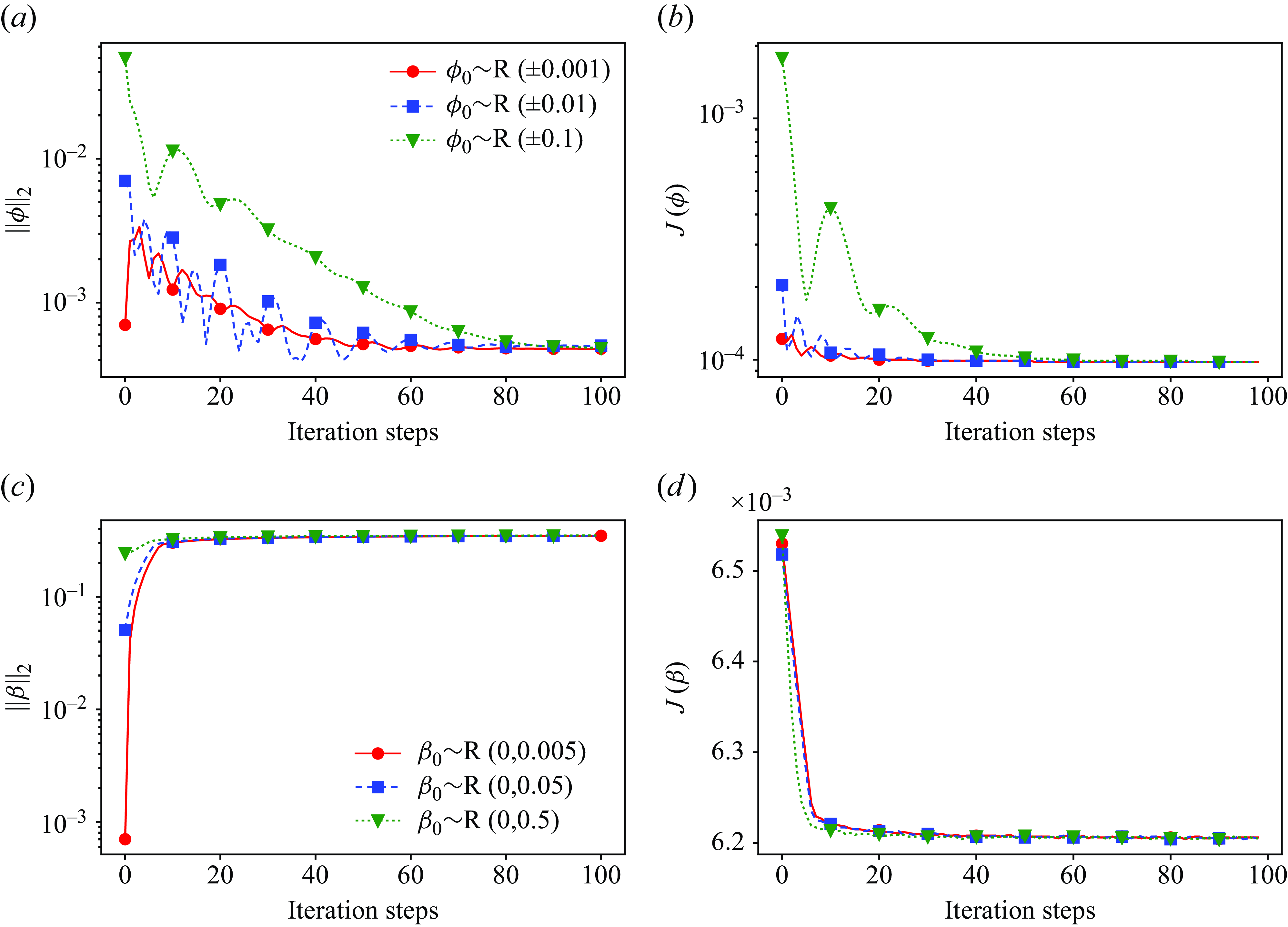
Figure 21. The sensitivity of the initial control field $\phi$
(terminal
$\phi$
(terminal $k$
control,
$k$
control, $\Delta t^+=25$
) and parameter
$\Delta t^+=25$
) and parameter $\beta$
(cumulative
$\beta$
(cumulative $\tau _w$
control,
$\tau _w$
control, $\Delta t^+=25$
). (a) The development of the
$\Delta t^+=25$
). (a) The development of the $L_2$
norm
$L_2$
norm $\|\phi \|_2$
with iteration steps for the opposition control case. (b) The evolution of the loss function
$\|\phi \|_2$
with iteration steps for the opposition control case. (b) The evolution of the loss function $J(\phi )$
with iteration steps. (c) The development of
$J(\phi )$
with iteration steps. (c) The development of $\|\beta \|_2$
with iteration steps for the permeable wall control case. (d) The evolution of the loss function
$\|\beta \|_2$
with iteration steps for the permeable wall control case. (d) The evolution of the loss function $J(\beta )$
with iteration steps.
$J(\beta )$
with iteration steps.
For the permeable wall control case, the initial parameter $\beta$
was also set as a uniformly distributed random field
$\beta$
was also set as a uniformly distributed random field $R$
with different limits, namely
$R$
with different limits, namely $(0,0.005)$
,
$(0,0.005)$
, $(0,0.05)$
and
$(0,0.05)$
and $(0,0.5)$
. The corresponding evolution of the
$(0,0.5)$
. The corresponding evolution of the $L_2$
norm
$L_2$
norm $\|\beta \|_2$
and the loss function
$\|\beta \|_2$
and the loss function $J(\beta )$
is shown in figures 21(c) and 21(d). Similar to the opposition control case, despite a two-order magnitude difference in the initial
$J(\beta )$
is shown in figures 21(c) and 21(d). Similar to the opposition control case, despite a two-order magnitude difference in the initial $\beta$
values, the optimisation consistently converged to the same final state.
$\beta$
values, the optimisation consistently converged to the same final state.
Despite variations in initial conditions, all cases exhibit stable convergence to the same final state, implying that the optimisation process is insensitive to the choice of initial parameters.
Appendix D. Decomposition of mean friction in permeable wall channels
Considering the channel flow, we assume statistical homogeneity in the spanwise and streamwise directions and symmetry with respect to the central plane of the channel. The compressible Reynolds-averaged momentum equation in the streamwise ( $x$
) direction is
$x$
) direction is
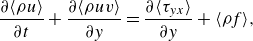 \begin{equation} \frac {\partial \langle \rho u\rangle }{\partial t}+\frac {\partial \langle \rho u v\rangle }{\partial y}=\frac {\partial \langle \tau _{y x} \rangle }{\partial y}+\langle \rho f\rangle, \end{equation}
where $u$
and
$u$
and $v$
are respectively the streamwise and wall-normal components of the transient velocity,
$v$
are respectively the streamwise and wall-normal components of the transient velocity, $\rho$
is density,
$\rho$
is density, $t$
is time and
$t$
is time and $\tau _{yx}$
is the shear stress in the streamwise direction. A uniform body force
$\tau _{yx}$
is the shear stress in the streamwise direction. A uniform body force $f$
is added to drive the flow in the streamwise direction. Integrating (D1) from the wall surface to the central plane gives
$f$
is added to drive the flow in the streamwise direction. Integrating (D1) from the wall surface to the central plane gives
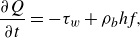 \begin{equation} \frac {\partial Q}{\partial t}=-\tau _w+\rho _b h f ,\end{equation}
where $Q$
is the mass flow rate across the traverse plane. In the current study,
$Q$
is the mass flow rate across the traverse plane. In the current study, $Q$
is controlled to be constant, hence
$Q$
is controlled to be constant, hence $f=\tau _w/\rho _bh$
.
$f=\tau _w/\rho _bh$
.
Rewriting the left-hand side of (D1) in the form of Favre average gives
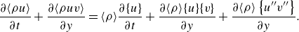 \begin{equation} \frac {\partial \langle \rho u\rangle }{\partial t}+\frac {\partial \langle \rho u v\rangle }{\partial y}=\langle \rho \rangle \frac {\partial \{u\}}{\partial t}+\frac {\partial \langle \rho \rangle \{u\}\{v\}}{\partial y}+\frac {\partial \langle \rho \rangle \left \{u^{\prime \prime } v^{\prime \prime }\right \}}{\partial y}. \end{equation}
For the no-slip boundary condition and zero-net-flux opposition control boundary condition, the second term on the right-hand side, representing the mean convection in the vertical direction, is considered as zero since $\{v\}=0$
. However, for the permeable wall condition, this term may not be zero as flux through the wall is allowed.
$\{v\}=0$
. However, for the permeable wall condition, this term may not be zero as flux through the wall is allowed.
Substituting (D2) and (D3) into (D1), we have
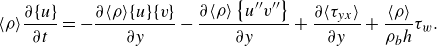 \begin{equation} \langle \rho \rangle \frac {\partial \{u\}}{\partial t}=-\frac {\partial \langle \rho \rangle \{u\}\{v\}}{\partial y}-\frac {\partial \langle \rho \rangle \left \{u^{\prime \prime } v^{\prime \prime }\right \}}{\partial y}+\frac {\partial \langle \tau _{y x} \rangle }{\partial y}+\frac {\langle \rho \rangle }{\rho _b h} \tau _w . \end{equation}
We convert the original reference frame, which is stationary with respect to the wall, into an absolute reference frame, travelling at velocity $u_b$
. Consequently, the friction on the wall generates a non-zero power that contributes to the mean kinetic energy budget. Let the subscript
$u_b$
. Consequently, the friction on the wall generates a non-zero power that contributes to the mean kinetic energy budget. Let the subscript $a$
represent the variables in the absolute frame. We have
$a$
represent the variables in the absolute frame. We have
 \begin{equation} t_a=t, \quad \rho _a=\rho , \quad x_a=x-u_b t, \quad y_a=y, \quad u_a=u-u_b, \quad v_a=v .\end{equation}
Substituting (D5) into (D4) yields
 \begin{equation} \langle \rho _a\rangle \frac {\partial \{u_a\}}{\partial t_a}=-\frac {\partial \langle \rho _a\rangle \{u_a\}\{v_a\}}{\partial y_a}-\frac {\partial \langle \rho _a\rangle \left \{u_a^{\prime \prime } v_a^{\prime \prime }\right \}}{\partial y_a}+\frac {\partial \langle \tau _{y x} \rangle }{\partial y_a}+\frac {\langle \rho _a\rangle }{\rho _b h} \tau _w . \end{equation}
Multiplying both sides of (D6) by $\{u_a\}$
, we have the energy budget equation
$\{u_a\}$
, we have the energy budget equation
 \begin{equation} \langle \rho _a \rangle \frac {\partial \left \{K_a\right \}}{\partial t_a}=-\left \{u_a\right \}\frac {\partial \langle \rho _a\rangle \{u_a\}\{v_a\}}{\partial y}-\left \{u_a\right \} \frac {\partial \langle \rho _a \rangle \left \{u_a^{\prime \prime } v_a^{\prime \prime }\right \}}{\partial y_a}+\left \{u_a\right \} \frac {\partial \langle \tau _{y x} \rangle }{\partial y_a}+\left \{u_a\right \} \frac { \langle \rho _a \rangle }{\rho _b h} \tau _w , \end{equation}
where $K_a=\{u_a\}^2/2$
is the averaged streamwise kinetic energy of unit mass in the absolute frame. For a channel flow statistically homogeneous in time,
$K_a=\{u_a\}^2/2$
is the averaged streamwise kinetic energy of unit mass in the absolute frame. For a channel flow statistically homogeneous in time, ${\partial K_a}/{\partial t_a}=0$
. A single integration over the half-channel is then performed on (D7), using symmetry boundary conditions at the centreline and
${\partial K_a}/{\partial t_a}=0$
. A single integration over the half-channel is then performed on (D7), using symmetry boundary conditions at the centreline and $\{u_a\}|_{y=0}=-u_b$
leads to the formula of the skin-friction coefficient in the absolute reference frame:
$\{u_a\}|_{y=0}=-u_b$
leads to the formula of the skin-friction coefficient in the absolute reference frame:
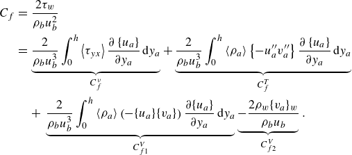 \begin{eqnarray} C_f &=& \frac {2 \tau _w}{\rho _b u_b^2}\nonumber\\&=& \underbrace {\frac {2}{\rho _b u_b^3} \int _0^h\left \langle \tau _{y x}\right \rangle \frac {\partial \left \{u_a\right \}}{\partial y_a} \textrm {d} y_a}_{C_{f}^\nu }+\underbrace {\frac {2}{\rho _b u_b^3} \int _0^h\left \langle \rho _a\right \rangle \left \{-u_a^{\prime \prime } v_a^{\prime \prime }\right \} \frac {\partial \left \{u_a\right \}}{\partial y_a} \textrm {d} y_a}_{C_{f}^T}\\ && + \underbrace {\frac {2}{\rho _b u_b^3} \int _0^h\left \langle \rho _a\right \rangle \left (-\{u_a\}\{ v_a\}\right ) \frac {\partial \{u_a\}}{\partial y_a} \textrm {d} y_a}_{C_{f1}^V}\underbrace {-\frac {2\rho _w \{ v_a\}_w}{\rho _b u_b}}_{C_{f2}^V}. \nonumber \end{eqnarray}
Rewriting (D8) as a function of the usual (wall) reference frame variables yields
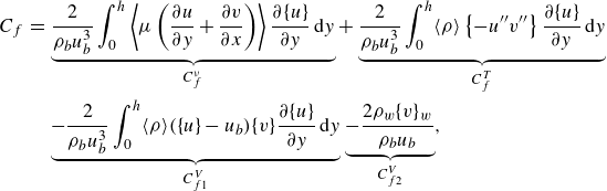 \begin{eqnarray} C_f &=& \underbrace {\frac {2}{\rho _b u_b^3} \int _0^h\left \langle \mu \left (\frac {\partial u}{\partial y}+\frac {\partial v}{\partial x}\right )\right \rangle \frac {\partial \{u\}}{\partial y} \textrm {d} y}_{C_{f}^\nu }+\underbrace {\frac {2}{\rho _b u_b^3} \int _0^h\langle \rho \rangle \left \{-u^{\prime \prime } v^{\prime \prime }\right \} \frac {\partial \{u\}}{\partial y} \textrm {d} y}_{C_{f }^T}\nonumber\\&& \underbrace {-\frac {2}{\rho _b u_b^3} \int _0^h\langle \rho \rangle (\{u\}-u_b)\{v\}\frac {\partial \{u\} }{\partial y} \textrm {d} y}_{C_{f1}^V}\underbrace {-\frac {2\rho _w \{ v\}_w}{\rho _b u_b}}_{C_{f2}^V}, \end{eqnarray}
where
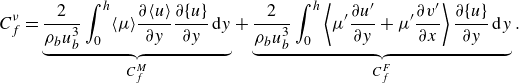 \begin{equation} C_{f}^{\nu }=\underbrace {\frac {2}{\rho _b u_b^3} \int _0^h\langle \mu \rangle \frac {\partial \langle u\rangle }{\partial y} \frac {\partial \{u\}}{\partial y} \textrm {d} y}_{C_{f}^M}+\underbrace {\frac {2}{\rho _b u_b^3} \int _0^h\left \langle \mu ^{\prime } \frac {\partial u^{\prime }}{\partial y}+\mu ^{\prime } \frac {\partial v^{\prime }}{\partial x}\right \rangle \frac {\partial \{u\}}{\partial y} \textrm {d} y}_{C_{f}^F} . \end{equation}
Here $C_{f}^{\nu }$
is associated with molecular viscosity dissipation,
$C_{f}^{\nu }$
is associated with molecular viscosity dissipation, $C_f^M$
is the mean shear term,
$C_f^M$
is the mean shear term, $C_f^F$
is the viscosity variation term,
$C_f^F$
is the viscosity variation term, $C_f^T$
the turbulent-convection term,
$C_f^T$
the turbulent-convection term, $C_{f1}^V$
and
$C_{f1}^V$
and $C_{f2}^{F}$
are mean convection terms that are generated due to the non-zero
$C_{f2}^{F}$
are mean convection terms that are generated due to the non-zero $\{v\}$
in the channel and at the wall.
$\{v\}$
in the channel and at the wall.


 Open access