


1. Introduction
Internal gravity waves observed in stably stratified fluids play an essential role in the transport of momentum, energy and mass in oceans, lakes and atmosphere. Therefore, different aspects related to the internal wave dynamics continue to be a subject of active research (e.g. Mathur & Peacock Reference Mathur and Peacock2010; Husseini et al. Reference Husseini, Varma, Dauxois, Joubaud, Odier and Mathur2020; Rodda et al. Reference Rodda, Savaro, Davis, Reneuve, Augier, Sommeria, Valran, Viboud and Mordan2022; Lanchon & Cortet Reference Lanchon and Cortet2023; Yalim et al. Reference Yalim, Welfert and Lopez2023). The structure of internal waves depends significantly on the stratification profile; waves at the interface separating two sufficiently thick layers of immiscible homogeneous liquids with different densities represent an important limiting case (Lamb Reference Lamb1932). The waves at a free water surface can be seen as a particular case of such a two-layer system when the density of the lighter fluid can be neglected.
The dispersion relation between the angular frequency $\omega$
and the horizontal wavevector
$\omega$
and the horizontal wavevector $\mathbf{k}$
for waves at a horizontally unlimited interface between two liquids with densities
$\mathbf{k}$
for waves at a horizontally unlimited interface between two liquids with densities $\rho _1\lt \rho _2$
is
$\rho _1\lt \rho _2$
is
 \begin{equation} \omega ^2=g'|\mathbf{k}|,\quad g'=g\frac {\rho _2-\rho _1}{\rho _2+\rho _1}, \end{equation}
where $g$
is the acceleration due to gravity. In the case of miscible liquids, a pycnocline separating the layers of constant density is formed where the density varies with the vertical coordinate
$g$
is the acceleration due to gravity. In the case of miscible liquids, a pycnocline separating the layers of constant density is formed where the density varies with the vertical coordinate $z$
, defining the local non-zero buoyancy frequency
$z$
, defining the local non-zero buoyancy frequency $N$
(Lighthill Reference Lighthill1978):
$N$
(Lighthill Reference Lighthill1978):
 \begin{equation} N^2(z)=-\frac {g}{\rho (z)}\frac {{\rm d}\rho (z)}{{\rm d}z}. \end{equation}
In this configuration more complex wave systems are possible. Time-dependent disturbances introduced in the bulk of one of the liquids may produce a superposition of symmetric and antisymmetric wavemodes propagating along the pycnocline (Davis & Acrivos Reference Davis and Acrivos1967b
). Antisymmetric solitary waves (sometimes referred to as mode-2 internal solitary waves) are observed in laboratory experiments (Davis & Acrivos Reference Davis and Acrivos1967a
; Cheng & Hsu Reference Cheng and Hsu2014; Deepwell & Stastna Reference Deepwell and Stastna2016), as well as in nature (Farmer & Smith Reference Farmer and Dungan Smith1980; Yang et al. Reference Yang, Fang, Chang, Ramp, Kao and Tang2009; Shanmugam Reference Shanmugam2013). The dispersion relation between the set of possible $\omega$
for any given
$\omega$
for any given $\mathbf{k}$
is defined by a solution of the Sturm–Liouville problem (Benjamin Reference Benjamin1967; Miles Reference Miles1971) and was approximated by Barber (Reference Barber1993).
$\mathbf{k}$
is defined by a solution of the Sturm–Liouville problem (Benjamin Reference Benjamin1967; Miles Reference Miles1971) and was approximated by Barber (Reference Barber1993).
In experiments on both surface and internal waves carried out in a closed laboratory facility, spatial confinement by vertical walls imposes limitations on possible wavevectors due to non-penetration boundary conditions (Thorpe Reference Thorpe1968; Faltinsen Reference Faltinsen1974; Geva et al. Reference Geva, Bukai, Zemach, Gabay, Krakovich and Shemer2021); in a deep narrow basin of length $L$
and width
$L$
and width $B\ll L$
, these wavevectors are
$B\ll L$
, these wavevectors are $\mathbf{k}=(k_n,0)$
,
$\mathbf{k}=(k_n,0)$
, $k_n=\pi n/L$
. The frequency of waves excited by externally controlled periodic motion of a rigid body is set by the forcing. In such experiments, a mismatch can exist between the forcing frequency
$k_n=\pi n/L$
. The frequency of waves excited by externally controlled periodic motion of a rigid body is set by the forcing. In such experiments, a mismatch can exist between the forcing frequency $\omega$
and eigenfrequencies prescribed by the reservoir geometry wavenumbers
$\omega$
and eigenfrequencies prescribed by the reservoir geometry wavenumbers $k_n$
via the dispersion relation (1.1). Additional adjustment of the eigenfrequencies is caused by the presence of the rigid wavemaker body within the liquid. The corresponding problem for a wavemaker-excited resonant standing surface gravity wave system in a narrow reservoir that accounts for the contribution of both the sidewalls and the wavemaker was solved by Mogilevskiy et al. (Reference Mogilevskiy, Kalenko, Zemach and Shemer2024). They demonstrated theoretically the existence of multiple spatial modes in the resonant wave spectrum, and validated those results in experiments.
$k_n$
via the dispersion relation (1.1). Additional adjustment of the eigenfrequencies is caused by the presence of the rigid wavemaker body within the liquid. The corresponding problem for a wavemaker-excited resonant standing surface gravity wave system in a narrow reservoir that accounts for the contribution of both the sidewalls and the wavemaker was solved by Mogilevskiy et al. (Reference Mogilevskiy, Kalenko, Zemach and Shemer2024). They demonstrated theoretically the existence of multiple spatial modes in the resonant wave spectrum, and validated those results in experiments.
The internal wavefield excited by a wavemaker in a deep narrow cavity filled by two liquids separated by a finite-thickness pycnocline is even more complicated. In this case, not only do multiple modes with different wavevectors coexist, but also for any given resonant wavenumber $k_n$
, modes with different vertical structures are possible. The internal structure within the pycnocline could not be captured in the study of wavemaker-excited resonant standing waves by Thorpe (Reference Thorpe1968) that was based on shadowgraph imaging. Since then, various optical methods have been applied to the study of internal waves, such as time-resolved particle image velocimetry (PIV) (Mathur & Peacock Reference Mathur and Peacock2010; Dossmann et al. Reference Dossmann, Paci, Auclair and Floor2011; Carr et al. Reference Carr, Davies and Hoebers2015; Boury et al. Reference Boury, Peacock and Odier2019), planar laser-induced fluorescence (Troy & Koseff Reference Troy and Koseff2005; Dossmann et al. Reference Dossmann, Bourget, Brouzet, Dauxois, Joubaud and Odier2016) and synthetic schlieren (Sutherland et al. Reference Sutherland, Dalziel, Hughes and Linden1999; Dalziel et al. Reference Dalziel, Hughes and Sutherland2000).
$k_n$
, modes with different vertical structures are possible. The internal structure within the pycnocline could not be captured in the study of wavemaker-excited resonant standing waves by Thorpe (Reference Thorpe1968) that was based on shadowgraph imaging. Since then, various optical methods have been applied to the study of internal waves, such as time-resolved particle image velocimetry (PIV) (Mathur & Peacock Reference Mathur and Peacock2010; Dossmann et al. Reference Dossmann, Paci, Auclair and Floor2011; Carr et al. Reference Carr, Davies and Hoebers2015; Boury et al. Reference Boury, Peacock and Odier2019), planar laser-induced fluorescence (Troy & Koseff Reference Troy and Koseff2005; Dossmann et al. Reference Dossmann, Bourget, Brouzet, Dauxois, Joubaud and Odier2016) and synthetic schlieren (Sutherland et al. Reference Sutherland, Dalziel, Hughes and Linden1999; Dalziel et al. Reference Dalziel, Hughes and Sutherland2000).
Modern video-based optical methods are applied here to study wavemaker-excited resonant standing waves in a narrow long basin within a pycnocline between two layers of liquids that slightly differ in density. This allows one to expand significantly the analysis of the system studied by Thorpe (Reference Thorpe1968) to reveal the effect of the pycnocline thickness on the complicated spatio-temporal structure of the internal wavefield within it. The experimental facility is described in § 2; in § 3, the analysis of the shadowgraph video recording is coupled with density profile measurements. These preliminary experiments prompted the development of a theoretical model based on the approach by Mogilevskiy et al. (Reference Mogilevskiy, Kalenko, Zemach and Shemer2024) in § 4. The theoretical prediction of the coexistence of symmetric and antisymmetric modes in the internal resonant standing wave within the pycnocline is verified quantitatively by PIV-derived data in § 5. Section 6 summarises the study.
2. Experimental set-up and shadowgraph procedure
Experiments were carried out in an $L=772$
mm long and
$L=772$
mm long and $B=160$
mm wide basin filled by layers of salted and pure water separated by a thin pycnocline. Stable stratification is attained by filling the basin first to a depth of 400 mm with MgCl
$B=160$
mm wide basin filled by layers of salted and pure water separated by a thin pycnocline. Stable stratification is attained by filling the basin first to a depth of 400 mm with MgCl $_{2}$
solution. Pure water is then gently added through a sponge that floats on the surface, until the total depth of the liquid in the basin reaches 700 mm. The densities of pure water (
$_{2}$
solution. Pure water is then gently added through a sponge that floats on the surface, until the total depth of the liquid in the basin reaches 700 mm. The densities of pure water ( $\rho _{1} =998.5$
kg m
$\rho _{1} =998.5$
kg m $^{-3}$
) and of the salt solution (
$^{-3}$
) and of the salt solution ( $\rho _{2}=1020$
kg m
$\rho _{2}=1020$
kg m $^{-3}$
) are measured using a Mettler Toledo densitometer. Inevitable mixing results in the formation of a finite-thickness pycnocline in which the density varies between its extreme values; the initial characteristic pycnocline thickness is about 14 mm. The density profile was determined with a high-precision conductivity probe (PCP) connected to a computer-controlled stage with a vertical resolution of 1 mm. The gradual increase of the actual thickness of the pycnocline in the course of experiments was monitored between the experimental runs by the PCP. A schematic sketch of the experimental set-up is presented in figure 1.
$^{-3}$
) are measured using a Mettler Toledo densitometer. Inevitable mixing results in the formation of a finite-thickness pycnocline in which the density varies between its extreme values; the initial characteristic pycnocline thickness is about 14 mm. The density profile was determined with a high-precision conductivity probe (PCP) connected to a computer-controlled stage with a vertical resolution of 1 mm. The gradual increase of the actual thickness of the pycnocline in the course of experiments was monitored between the experimental runs by the PCP. A schematic sketch of the experimental set-up is presented in figure 1.
Waves were excited by a cylinder $2R=42$
mm in diameter; its axis is horizontal and spans the whole width of the basin. The wavemaker is supported by a thin rod connected to a linear computer-controlled motor that generates vertical harmonic oscillations. The mean position of the wavemaker centre is 350 mm above the bottom of the basin in the heavier layer. The instantaneous vertical position was recorded using a laser position sensor and served as a phase reference.
$2R=42$
mm in diameter; its axis is horizontal and spans the whole width of the basin. The wavemaker is supported by a thin rod connected to a linear computer-controlled motor that generates vertical harmonic oscillations. The mean position of the wavemaker centre is 350 mm above the bottom of the basin in the heavier layer. The instantaneous vertical position was recorded using a laser position sensor and served as a phase reference.
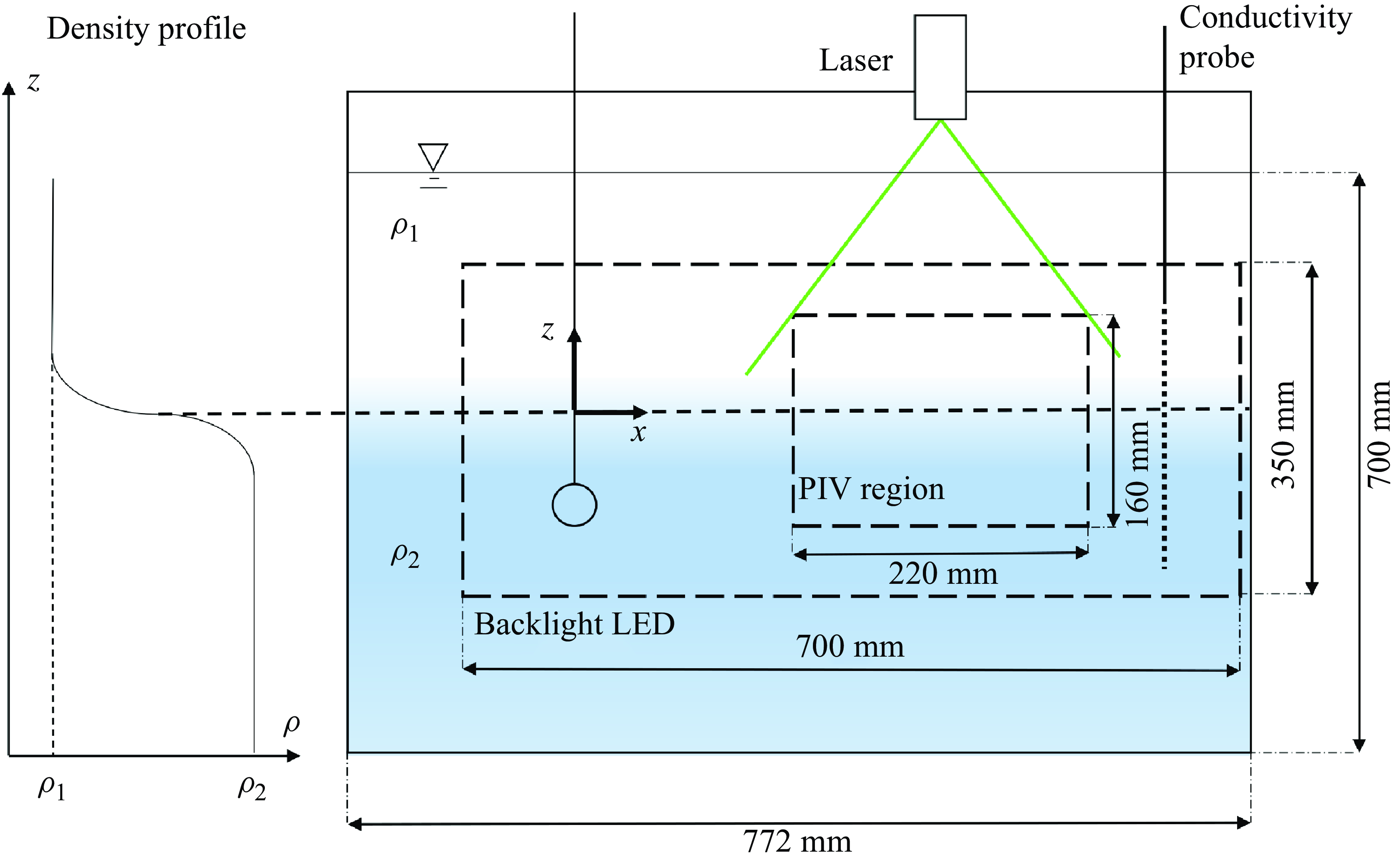
Figure 1. Sketch of the experimental system (front view); the basin is 160 mm wide. The origin of axes: $x=0$
at the wavemaker location;
$x=0$
at the wavemaker location; $z=0$
at the maximum of the density gradient at rest.
$z=0$
at the maximum of the density gradient at rest.
The two-layer model predicts the standing-wave frequency for the $n$
th spatial mode as
$n$
th spatial mode as
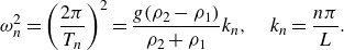 \begin{equation} \omega _n^2=\left (\frac {2\pi }{T_n}\right )^2=\frac {g(\rho _{2}-\rho _{1})}{\rho _{2}+\rho _{1}}k_n,\quad k_n=\frac {n\pi }{L}. \end{equation}
Mostly, the experiments were performed for $n=3$
and some of them for
$n=3$
and some of them for $n=4$
corresponding to oscillation periods of
$n=4$
corresponding to oscillation periods of $T_3=5.56$
s and
$T_3=5.56$
s and $T_4=4.85$
s, and wavelengths
$T_4=4.85$
s, and wavelengths $\lambda _3=514$
mm and
$\lambda _3=514$
mm and $\lambda _4=386$
mm. For both modes, the effects of the bottom and of the free surface of the lighter liquid are negligible as the thicknesses of both layers are sufficiently large (
$\lambda _4=386$
mm. For both modes, the effects of the bottom and of the free surface of the lighter liquid are negligible as the thicknesses of both layers are sufficiently large ( $D_{1,2}\gt 300$
mm); the resulting correction to the dispersion relation (2.1) does not exceed 0.2 %. The centre of the wavemaker was positioned at the antinode of the corresponding resonant mode, at a distance
$D_{1,2}\gt 300$
mm); the resulting correction to the dispersion relation (2.1) does not exceed 0.2 %. The centre of the wavemaker was positioned at the antinode of the corresponding resonant mode, at a distance $L/3$
from the sidewall for the experiments at
$L/3$
from the sidewall for the experiments at $n=3$
and
$n=3$
and $L/2$
for those at
$L/2$
for those at $n=4$
.
$n=4$
.
Preliminary experiments were carried out to determine the frequency range of maximum response. After that, a detailed frequency scan was performed. Those preliminary experiments clearly indicated that significant amplitudes of the internal waves are observed for frequencies below $\omega _n$
in the typical range of the normalised frequency:
$\omega _n$
in the typical range of the normalised frequency:
 \begin{align} 0.88\lt \alpha =\frac {\omega }{\omega _n}\lt 0.97. \end{align}
Each experimental run for prescribed wavemaker amplitude $F$
and normalised frequency
$F$
and normalised frequency $\alpha$
starts with the liquid at rest. The wavemaker operation lasts for about 30 min (300 periods). The wavemaker then stops and the recording continues until the waves practically vanish due to dissipation. The run finished with the measurement of the density profile by the PCP. The whole experiment is fully automated with LabView software that controls and synchronises the operation of all elements and data recording.
$\alpha$
starts with the liquid at rest. The wavemaker operation lasts for about 30 min (300 periods). The wavemaker then stops and the recording continues until the waves practically vanish due to dissipation. The run finished with the measurement of the density profile by the PCP. The whole experiment is fully automated with LabView software that controls and synchronises the operation of all elements and data recording.
Figure 2 describes the evolution of the density distribution during a series of 12 experimental runs for $n=3$
with 12 equally spaced frequencies ranging from
$n=3$
with 12 equally spaced frequencies ranging from $\alpha _{min}=0.89$
to
$\alpha _{min}=0.89$
to $\alpha _{max}=0.94$
;
$\alpha _{max}=0.94$
; $F =7.5$
mm. Density profiles measured prior to the first run and following the last run are plotted in figure 2(a). During the course of the experiment, the thickness of the pycnocline grows; it is defined as
$F =7.5$
mm. Density profiles measured prior to the first run and following the last run are plotted in figure 2(a). During the course of the experiment, the thickness of the pycnocline grows; it is defined as
 \begin{equation} d =\frac {(\rho _{2}-\rho _{1})}{|{\rm d} \rho / {\rm d}z|_{max}}, \end{equation}
where $|d \rho / d z|_{max}$
is the density gradient maximum (figure 2
b). Note that the measurements of the density profile performed repeatedly each 30 min in a constantly stagnant liquid with the wavemaker at rest during 12 hours demonstrated negligible change in
$|d \rho / d z|_{max}$
is the density gradient maximum (figure 2
b). Note that the measurements of the density profile performed repeatedly each 30 min in a constantly stagnant liquid with the wavemaker at rest during 12 hours demonstrated negligible change in $d$
due to molecular diffusion. Indeed, for a diffusion coefficient
$d$
due to molecular diffusion. Indeed, for a diffusion coefficient $\kappa \sim 10^{-3}$
mm
$\kappa \sim 10^{-3}$
mm $^2$
s−1, the estimate of the widening of the pycnocline with time
$^2$
s−1, the estimate of the widening of the pycnocline with time $t$
as
$t$
as $d^2(t)-d^2(t_0)\sim \kappa (t-t_0)$
yields the growth of the pycnocline thickness
$d^2(t)-d^2(t_0)\sim \kappa (t-t_0)$
yields the growth of the pycnocline thickness $d$
that is below 10 %.
$d$
that is below 10 %.
The density gradient distribution characterised by the buoyancy frequency (1.2) becomes wider with a corresponding decrease of the maximum $N^2_{max}$
(figure 2
c). However, the shape of the normalised profiles
$N^2_{max}$
(figure 2
c). However, the shape of the normalised profiles $N^2(z/d)/N^2_{max}$
does not change notably and is well approximated by a Gaussian (figure 2
d):
$N^2(z/d)/N^2_{max}$
does not change notably and is well approximated by a Gaussian (figure 2
d):
 \begin{equation} N^2=\frac {2g(\rho _2-\rho _1)}{d(\rho _2+\rho _1)}\exp \left (-\pi \frac {z^2}{d^2}\right )=2\frac {(\omega _n)^2}{k_nd}\exp \left (-\pi \frac {z^2}{d^2}\right ). \end{equation}
The non-dimensional buoyancy frequency is defined as
 \begin{equation} {\tilde {N}}^2=\frac {2}{\delta }\exp \left (-\pi \frac {z^2}{d^2}\right ),\quad \delta =k_nd. \end{equation}
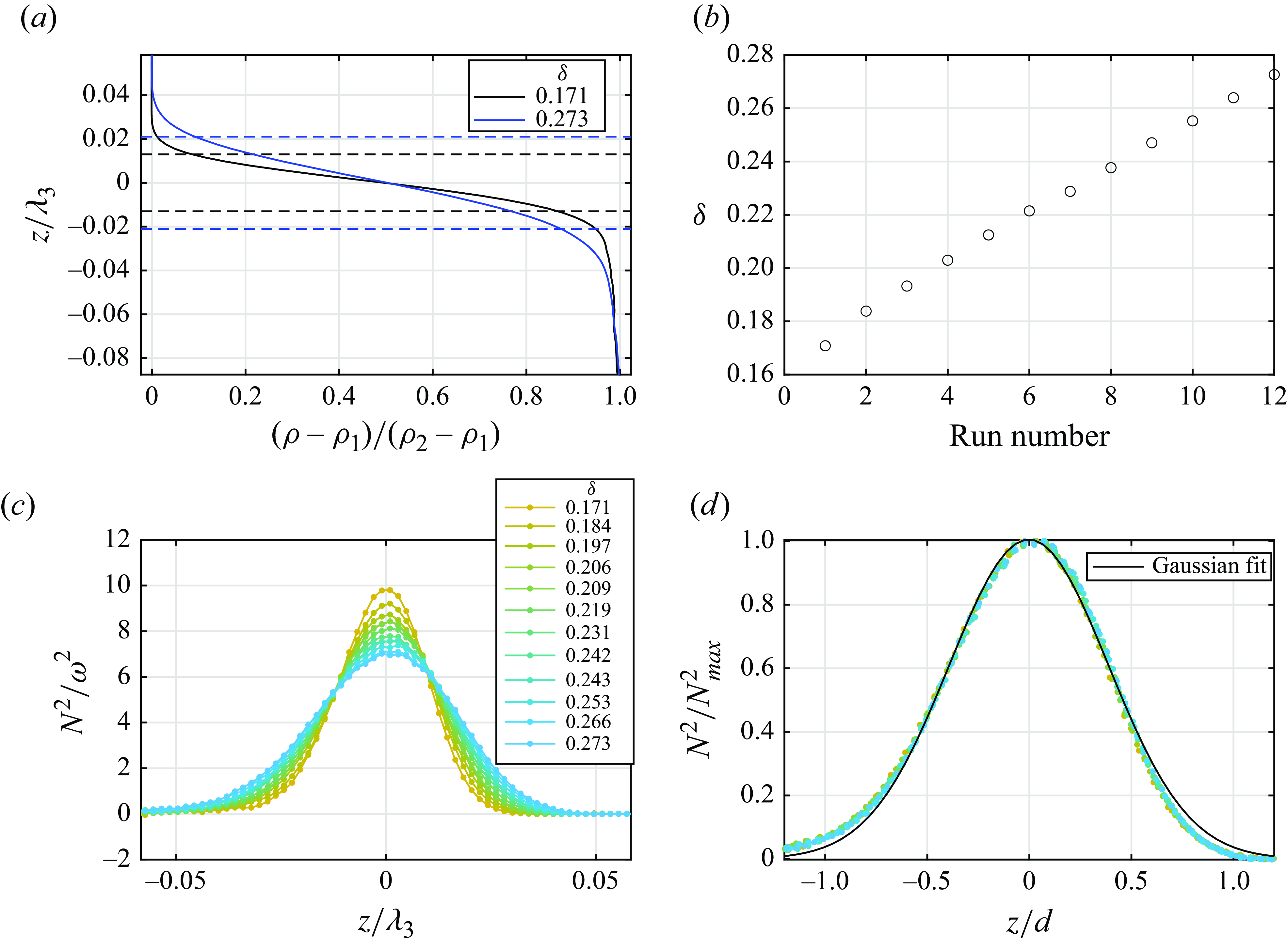
Figure 2. Density profile evolution during experiments at $F=7.5$
mm, and
$F=7.5$
mm, and $0.89 \leqslant \alpha \leqslant 0.94$
. (a) The measured extreme density profiles. The dashed horizontal lines mark the effective pycnocline boundaries
$0.89 \leqslant \alpha \leqslant 0.94$
. (a) The measured extreme density profiles. The dashed horizontal lines mark the effective pycnocline boundaries $\pm d/(2\lambda _3$
). (b) The variation of the dimensionless pycnocline thickness
$\pm d/(2\lambda _3$
). (b) The variation of the dimensionless pycnocline thickness $\delta$
as a function of run number. (c) Corresponding distributions of buoyancy frequency. (d) Collapse of the normalised distributions. This and subsequent figures correspond to
$\delta$
as a function of run number. (c) Corresponding distributions of buoyancy frequency. (d) Collapse of the normalised distributions. This and subsequent figures correspond to $n=3$
, unless specified explicitly otherwise.
$n=3$
, unless specified explicitly otherwise.
Experiments were first performed using the shadowgraph technique that gives wide spatial coverage; after that, the internal structure of the waves was extracted using PIV data.
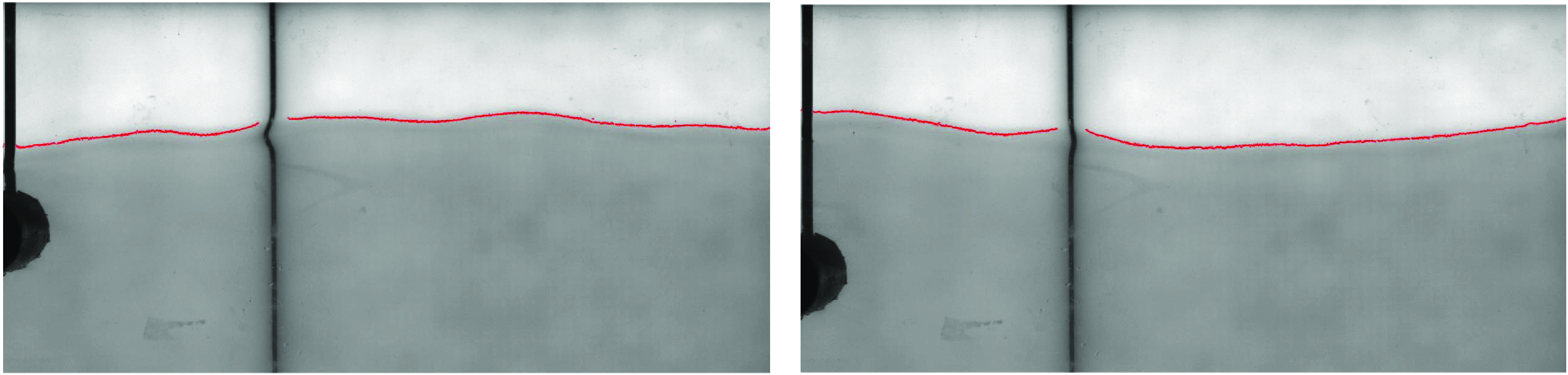
Figure 3. Two shadowgraph images shifted in time by half a wavemaker period. Supplementary movie 1 available at https://doi.org/10.1017/jfm.2025.384 shows the movement of the detected interface.
3. Shadowgraph experiments
For shadowgraph experiments, a fluorescent dye added to the heavier fluid forms a distinct boundary in the images (figure 3). Two back-light square LED panels adjacent to the back wall of the basin provide uniform illumination over the total area of 350 mm $\times$
700 mm which is captured by a camera (3.2 MPixel USB 3.1 Flir Blackfly) at 10 frames per second. The location of the sharp interface clearly visible in figure 1 was extracted using an edge-detection procedure. The LED panel joint and the rod supporting the wavemaker cause two small gaps where the interface location cannot be determined.
$\times$
700 mm which is captured by a camera (3.2 MPixel USB 3.1 Flir Blackfly) at 10 frames per second. The location of the sharp interface clearly visible in figure 1 was extracted using an edge-detection procedure. The LED panel joint and the rod supporting the wavemaker cause two small gaps where the interface location cannot be determined.
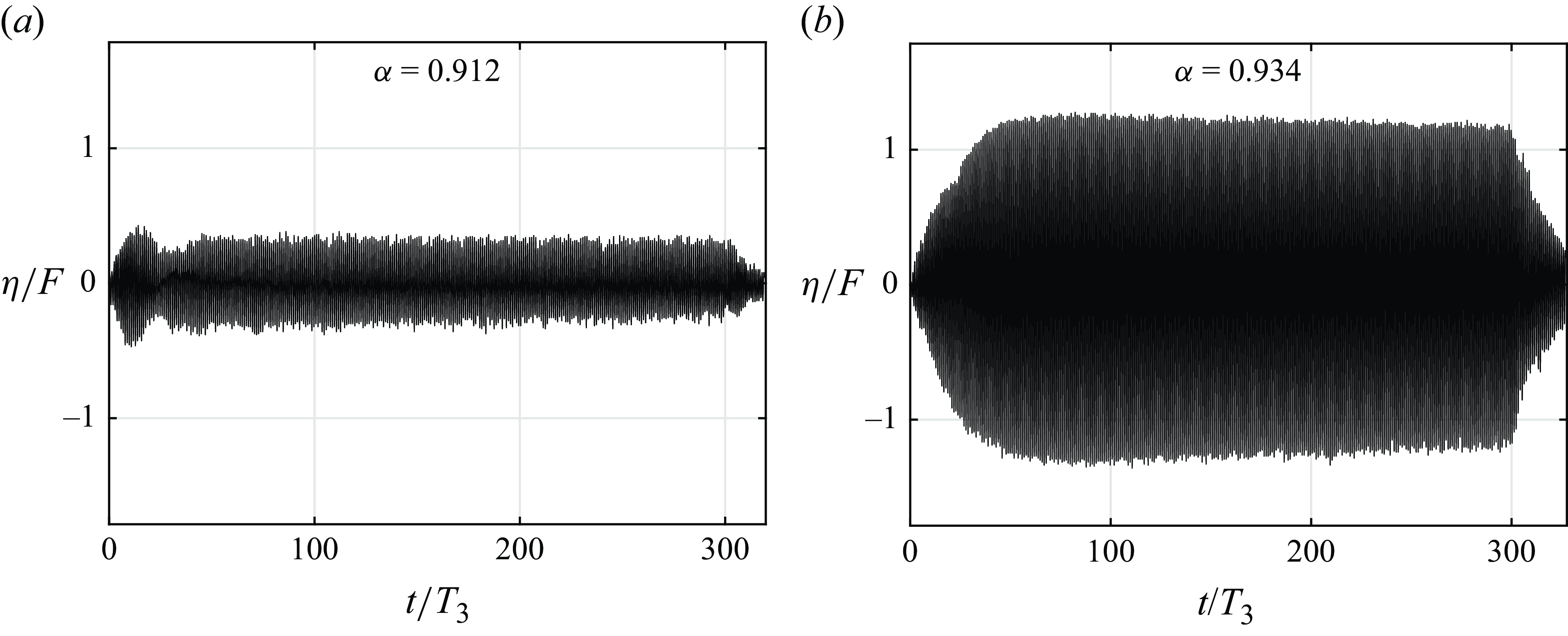
Figure 4. Dimensionless interface elevation $\eta /F$
at antinode (
$\eta /F$
at antinode ( $x/\lambda _3=0.5$
) of the third mode as a function of time, for wavemaker amplitude
$x/\lambda _3=0.5$
) of the third mode as a function of time, for wavemaker amplitude $F =5.6$
mm and (a,b) different forcing frequencies.
$F =5.6$
mm and (a,b) different forcing frequencies.
The comparison of the processed images with the PCP data demonstrated that the interface location $z=\zeta (t,x)$
in the images corresponds to the upper edge of the pycnocline. Figure 4 shows the normalised interface elevation
$z=\zeta (t,x)$
in the images corresponds to the upper edge of the pycnocline. Figure 4 shows the normalised interface elevation
 \begin{align} \eta (t,x)=\zeta (t,x)-\zeta (0,x) \end{align}
at the antinode of the third mode ( $x/\lambda _3=0.5$
) for the wavemaker amplitude
$x/\lambda _3=0.5$
) for the wavemaker amplitude $F$
$F$ $ =5.6$
mm as a function of time for two forcing frequencies;
$ =5.6$
mm as a function of time for two forcing frequencies; $\alpha =0.93$
(figure 4
b) corresponds to the effective resonance. The initial transient stage lasts about 25–50 periods of wavemaker oscillations and is followed by a quasi-steady stage. The slow variation of the wave amplitude at this stage can be attributed to the growth of the mixing layer in the course of the run. The termination of the wavemaker operation results in a decay of waves at a time scale comparable with that of the initial transient stage.
$\alpha =0.93$
(figure 4
b) corresponds to the effective resonance. The initial transient stage lasts about 25–50 periods of wavemaker oscillations and is followed by a quasi-steady stage. The slow variation of the wave amplitude at this stage can be attributed to the growth of the mixing layer in the course of the run. The termination of the wavemaker operation results in a decay of waves at a time scale comparable with that of the initial transient stage.
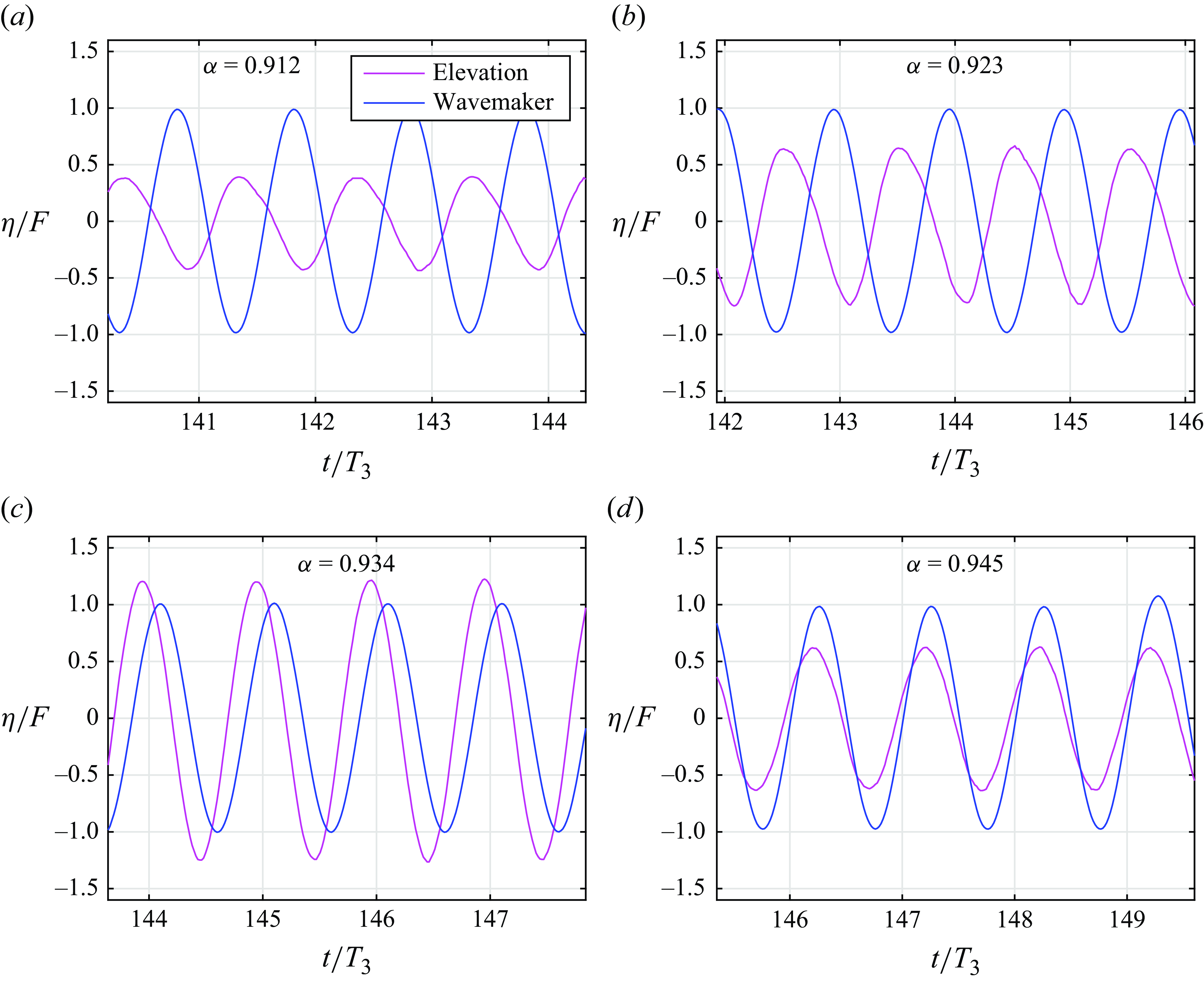
Figure 5. Short simultaneous records of interface elevation at the third-mode antinode $x/\lambda _3=0.5$
and wavemaker movement for(a–d) different forcing frequencies; experimental conditions as in figure 4.
$x/\lambda _3=0.5$
and wavemaker movement for(a–d) different forcing frequencies; experimental conditions as in figure 4.
3.1. Results of the measurements
The apparently sinusoidal temporal variation of the interface elevation above the wavemaker is plotted in figure 5 together with the records of the wavemaker motion at different forcing frequencies. An effective resonance is observed at $\alpha$
about 0.93; at lower frequencies, the interface oscillations at this lateral location are approximately in antiphase relative to the wavemaker motion. The phase difference seems to decrease notably as the forcing frequency exceeds the effective resonance; in figure 5(d), the oscillations are nearly in phase.
$\alpha$
about 0.93; at lower frequencies, the interface oscillations at this lateral location are approximately in antiphase relative to the wavemaker motion. The phase difference seems to decrease notably as the forcing frequency exceeds the effective resonance; in figure 5(d), the oscillations are nearly in phase.


Several instantaneous interface shapes are plotted in figure 6(a). While those shapes indeed seem to be dominated by the resonant standing wave with $m=3$
, they clearly contain contributions from additional shorter waves. The appearance of shorter waves is more pronounced for frequencies below the resonant frequency (dashed curves in figure 6
a). The root-mean-square
$m=3$
, they clearly contain contributions from additional shorter waves. The appearance of shorter waves is more pronounced for frequencies below the resonant frequency (dashed curves in figure 6
a). The root-mean-square $\langle \eta ^2\rangle ^{1/2}$
values of the interface elevation were calculated separately for each horizontal location
$\langle \eta ^2\rangle ^{1/2}$
values of the interface elevation were calculated separately for each horizontal location $x$
(figure 6
b) and averaged over 220 periods corresponding to the quasi-steady state. For a monochromatic standing wave, the expected values of
$x$
(figure 6
b) and averaged over 220 periods corresponding to the quasi-steady state. For a monochromatic standing wave, the expected values of $\langle \eta ^2 \rangle ^{1/2}$
are zero at nodes spaced by half a wavelength, and reach their maximum at antinodes. Figure 6(b) demonstrates that this pattern describes the actual behaviour only approximately; the values of
$\langle \eta ^2 \rangle ^{1/2}$
are zero at nodes spaced by half a wavelength, and reach their maximum at antinodes. Figure 6(b) demonstrates that this pattern describes the actual behaviour only approximately; the values of $\langle \eta ^2 \rangle ^{1/2}$
do not vanish at nodes, and the shapes around the antinodes are quite flat. At frequencies well below the effective resonance, the measured distributions of
$\langle \eta ^2 \rangle ^{1/2}$
do not vanish at nodes, and the shapes around the antinodes are quite flat. At frequencies well below the effective resonance, the measured distributions of $\langle \eta ^2 \rangle ^{1/2}$
are nearly flat everywhere. The complexity of the interface wavy shape manifests itself in the wavenumber spectra of the complex amplitude of the interface shape band-pass-filtered at the forcing frequency (figure 7). Along with the global maxima at
$\langle \eta ^2 \rangle ^{1/2}$
are nearly flat everywhere. The complexity of the interface wavy shape manifests itself in the wavenumber spectra of the complex amplitude of the interface shape band-pass-filtered at the forcing frequency (figure 7). Along with the global maxima at $m=3$
, the additional weaker local maxima at
$m=3$
, the additional weaker local maxima at $m\approx 9$
and
$m\approx 9$
and $m\approx 15$
are seen. The former can be attributed to the cubic nonlinearity and the interaction of the dominant wavemode with itself, while the latter has no analogy in the surface waves.
$m\approx 15$
are seen. The former can be attributed to the cubic nonlinearity and the interaction of the dominant wavemode with itself, while the latter has no analogy in the surface waves.

The frequency spectrum of the interface elevation at the antinode is dominated by a harmonic at the wavemaker driving frequency (figure 8 a); this harmonic, while much weaker, is also notable at the node of the standing wave (figure 8 b). At both the node and the antinode, there is a significant peak at double the wavemaker frequency, which is more pronounced when the forcing frequency is below the effective resonance (figure 8 a).
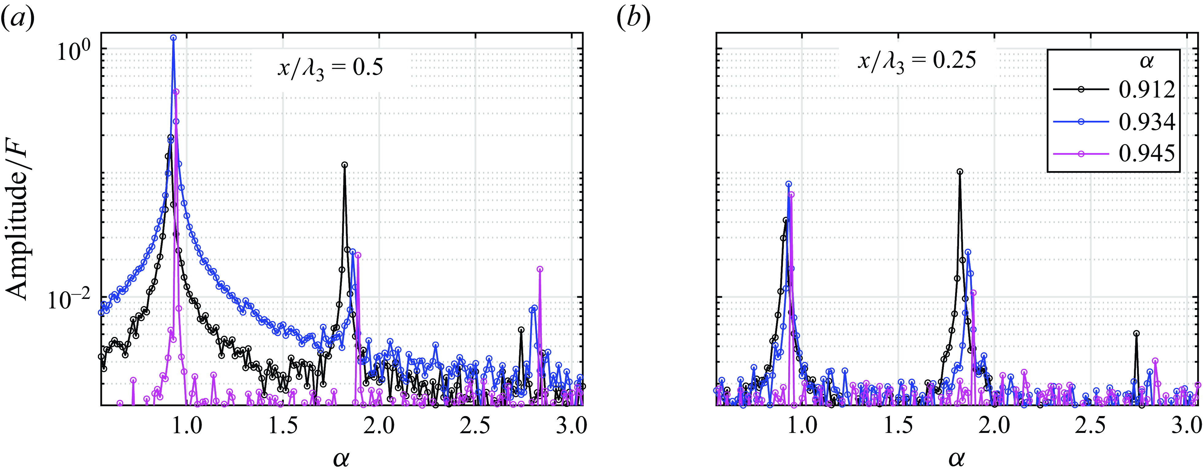
Figure 8. Normalised amplitude frequency spectra of interface elevation for wavemaker amplitude $F =5.6$
mm: (a) at the antinode (
$F =5.6$
mm: (a) at the antinode ( $x/\lambda _3=0.5$
); (b) at the node (
$x/\lambda _3=0.5$
); (b) at the node ( $x/\lambda _3=0.25$
).
$x/\lambda _3=0.25$
).
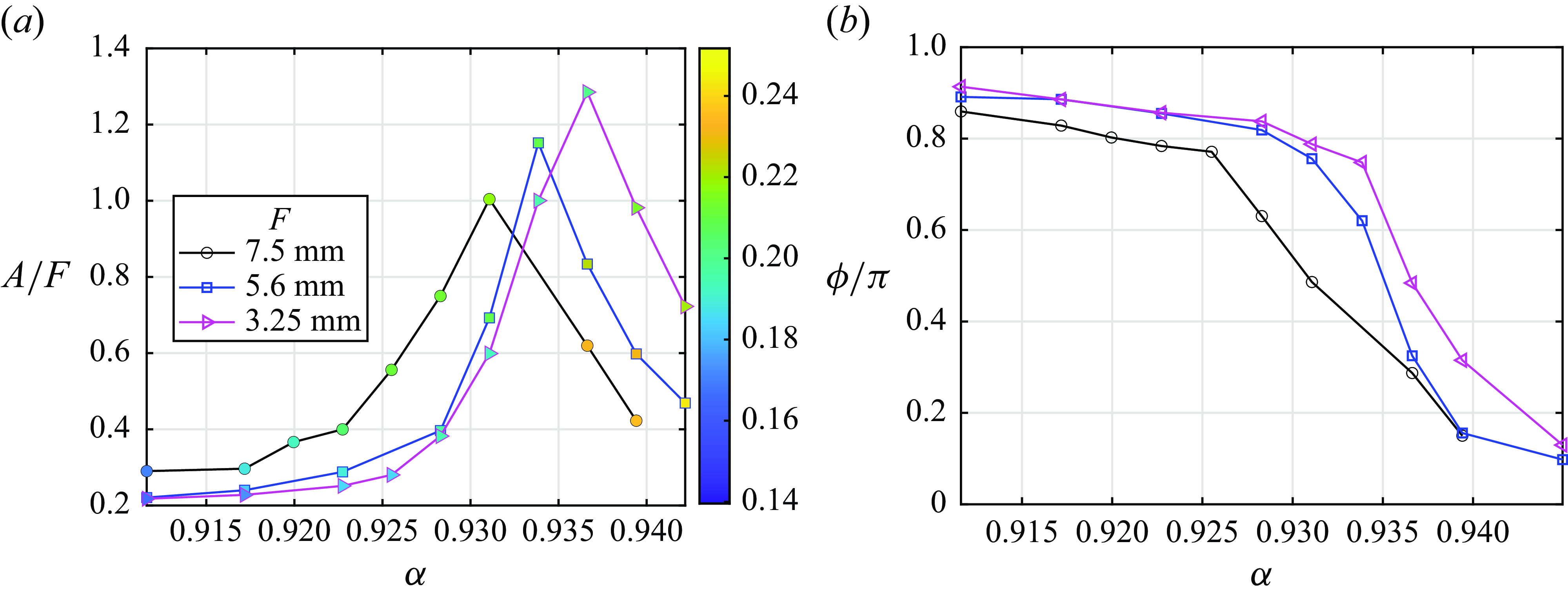
Figure 9. (a) Interface elevation amplitude in the antinode ( $x/\lambda _3=0.5$
) for different forcing amplitudes, the coloured symbols represent the pycnocline thickness
$x/\lambda _3=0.5$
) for different forcing amplitudes, the coloured symbols represent the pycnocline thickness $\delta$
. (b) Phase difference between the surface elevation and the wavemaker displacement for the cases as in (a).
$\delta$
. (b) Phase difference between the surface elevation and the wavemaker displacement for the cases as in (a).
The variation of the amplitude of the interface elevation with forcing frequency is plotted in figure 9(a) for three values of the wavemaker amplitude obtained in a single series of experimental runs with increasing forcing frequency. The effective resonance downshifts as the forcing amplitude increases. The pycnocline thickness $d$
grows so that
$d$
grows so that $\delta$
changes from about
$\delta$
changes from about $0.17$
to about
$0.17$
to about $0.25$
as shown in figure 9 by colours of the markers. The decrease of the phase shift between the interface elevation above the wavemaker and the wavemaker from
$0.25$
as shown in figure 9 by colours of the markers. The decrease of the phase shift between the interface elevation above the wavemaker and the wavemaker from $\pi$
towards zero is plotted for those runs in figure 9(b).
$\pi$
towards zero is plotted for those runs in figure 9(b).
The effect of the pycnocline thickness widening in the course of the experiment is studied in an additional series of experiments carried out for $n=4$
. Those runs started from the lowest frequency with
$n=4$
. Those runs started from the lowest frequency with $\alpha =0.92$
, attained the value of forcing frequency
$\alpha =0.92$
, attained the value of forcing frequency $\alpha =0.978$
, after which the values of
$\alpha =0.978$
, after which the values of $\alpha$
were gradually decreased. Figure 10 shows the downshift of the resonant frequency with an increase of
$\alpha$
were gradually decreased. Figure 10 shows the downshift of the resonant frequency with an increase of $\delta$
.
$\delta$
.
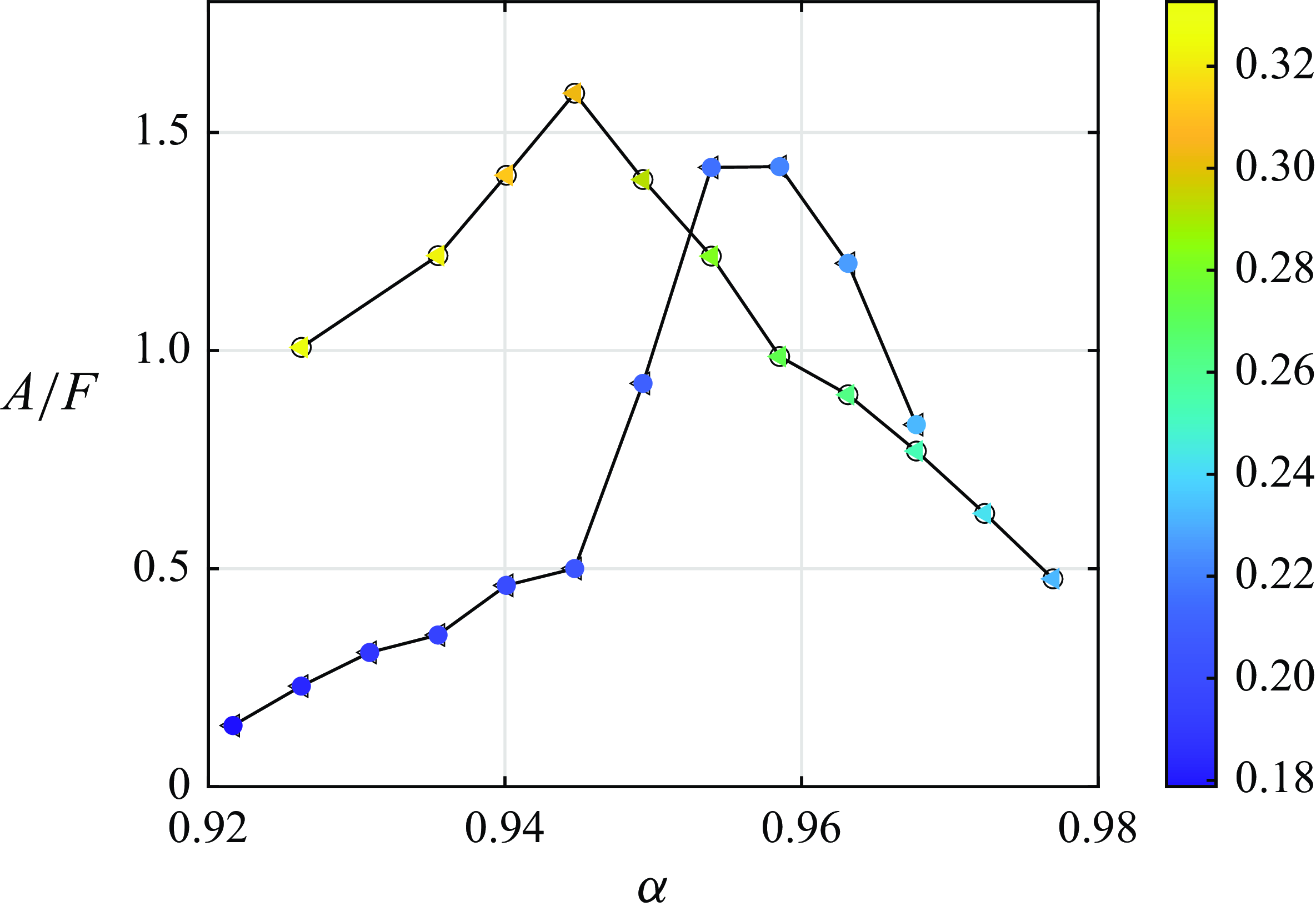
Figure 10. Interface elevation amplitude at the antinode ( $n=4$
,
$n=4$
, $x/\lambda _4=0.25$
,
$x/\lambda _4=0.25$
, $F=10$
mm). The coloured symbols represent the pycnocline thickness
$F=10$
mm). The coloured symbols represent the pycnocline thickness $\delta$
.
$\delta$
.
3.2. Interim conclusions
Shadowgraph experiments reveal the basic features of internal waves in a closed basin containing two liquids with different densities separated by a relatively thin pycnocline. The complex structure of the wave, excited by a wavemaker operating in the vicinity of the resonant frequency corresponding to the selected two-layer mode, is exposed in the temporal records of the visible interface elevation. The temporal spectra at any longitudinal location are dominated by discrete harmonics corresponding to the wavemaker forcing frequency $\omega$
and its second harmonic 2
$\omega$
and its second harmonic 2 $\omega$
. The resonant wave in the vicinity of the third-mode resonant frequency clearly deviates from the sinusoidal shape: the wavenumber spectra of records band-pass-filtered at the forcing frequency (figure 7) contain multiple components with
$\omega$
. The resonant wave in the vicinity of the third-mode resonant frequency clearly deviates from the sinusoidal shape: the wavenumber spectra of records band-pass-filtered at the forcing frequency (figure 7) contain multiple components with $m$
in the vicinity of the resonant mode
$m$
in the vicinity of the resonant mode $n=3$
, components with
$n=3$
, components with $m\approx 3n$
that may be attributed to cubic nonlinearity and
$m\approx 3n$
that may be attributed to cubic nonlinearity and $m\approx 15$
that, as will be shown in the following, are related to the finite pycnocline thickness. The effective resonance frequency in the experiments is apparently downshifted from the two-layer model prediction
$m\approx 15$
that, as will be shown in the following, are related to the finite pycnocline thickness. The effective resonance frequency in the experiments is apparently downshifted from the two-layer model prediction $\omega _n$
; this downshift increases with an increase of the wavemaker amplitude
$\omega _n$
; this downshift increases with an increase of the wavemaker amplitude $F$
.
$F$
.
The thickness of the pycnocline $d$
increases in the course experimental sessions. The increase in
$d$
increases in the course experimental sessions. The increase in $d$
affects notably the effective resonance of the system; it also contributes to the downshift of the effective resonant frequency. It should be emphasised that while the density distribution can be monitored between the runs using the PCP, there is no way to control it.
$d$
affects notably the effective resonance of the system; it also contributes to the downshift of the effective resonant frequency. It should be emphasised that while the density distribution can be monitored between the runs using the PCP, there is no way to control it.
The shadowgraph experiments have the advantage of wide spatial coverage, but the sequence of recorded images only provides information on the movement of one surface representing the effective interface. This technique is thus incapable of revealing the full internal wave structure inside a pycnocline of finite thickness, suggesting that a different experimental approach is needed. The PIV technique can provide the necessary two-dimensional information; however, carrying out these experiments for a wide range of parameters requires extensive resources. An efficient experimental programme can benefit from guidelines supplied by a theoretical model that gives prior estimates of the wavefield behaviour.
4. Theoretical model
Modelling of surface water waves is routinely based on the assumption of irrotational flow within the liquid governed by the Laplace equation; due to the Green theorem once the free-surface boundary conditions are satisfied, the flow in the bulk can be computed (see e.g. Newman Reference Newman2018). For stratified media, neglecting the thickness of the pycnocline results in the two-layer model with the dispersion relation (1.1) for linear waves (Lamb Reference Lamb1932). Methods developed for accounting for nonlinear effects associated with the finite wave amplitude (e.g. Penny Reference Penny1952) applied to a two-layer model by Thorpe (Reference Thorpe1968) showed the appearance of a bound wave with double wavenumber and frequency and a decrease of the wave celerity associated with the wave steepness. The generalisation of this approach to account for continuous stratification by Miles (Reference Miles1986) resulted in a variational formulation capable of describing weakly nonlinear propagating waves in arbitrary stably stratified pycnoclines. The similarity between the surface and the internal waves within the two-layer model enables estimates of the effect of the internal wave amplitude using the results obtained for resonantly forced surface waves (Moiseev Reference Moiseev1958; Faltinsen Reference Faltinsen1974; Mogilevskiy et al. Reference Mogilevskiy, Kalenko, Zemach and Shemer2024).
The internal wavefield structure is affected by the finite pycnocline thickness at any wave amplitude. As shown by Miles (Reference Miles1971), the flow within the pycnocline is not potential; thus, the dispersion relation cannot be obtained explicitly. It can be obtained by solving the Sturm–Liouville problem for a given density distribution. Besides, continuous stratification does not allow introduction of a distinct horizontal boundary where boundary conditions can be stated as in the two-layer model.
In this section, the resonant surface wave model (Mogilevskiy et al. Reference Mogilevskiy, Kalenko, Zemach and Shemer2024) is first adjusted to a two-layer system. Then, an analytical solution is presented for continuous stratification approximated by a piecewise-constant profile of the buoyancy frequency $N^2(z)$
, while neglecting the wavemaker size. Finally, a numerical method that accounts for viscous dissipation, arbitrary stratification and the wavemaker geometry is introduced.
$N^2(z)$
, while neglecting the wavemaker size. Finally, a numerical method that accounts for viscous dissipation, arbitrary stratification and the wavemaker geometry is introduced.
4.1. Two-layer model
Consider two-dimensional flow in the $(x,z)$
plane of two effectively infinite deep layers of homogeneous liquids separated by interface
$(x,z)$
plane of two effectively infinite deep layers of homogeneous liquids separated by interface $z=\eta (x,t)$
. The variables are rendered dimensionless as
$z=\eta (x,t)$
. The variables are rendered dimensionless as
 \begin{align} (\tilde {x},{\tilde {z}})=k_n(x,z),\quad \tilde {t}=\omega t .\end{align}
The velocity is scaled by $\omega F$
; the interface location by
$\omega F$
; the interface location by $F$
:
$F$
:
 \begin{align} \tilde {\eta }=\frac {\eta }{F }. \end{align}
The dimensionless wall locations are $\tilde {x}=-\pi$
and
$\tilde {x}=-\pi$
and $\tilde {x}=(n-1)\pi$
. The mean position of the interface is
$\tilde {x}=(n-1)\pi$
. The mean position of the interface is $\tilde {\eta }=0$
. The dimensionless parameters
$\tilde {\eta }=0$
. The dimensionless parameters $r$
and
$r$
and $h$
,
$h$
,
 \begin{align} r=k_nR,\quad h=k_nH, \end{align}
define the geometry of the wavemaker; $-H$
is the mean vertical coordinate of its centre. For
$-H$
is the mean vertical coordinate of its centre. For $n=3$
, the experiments correspond to
$n=3$
, the experiments correspond to $r=0.26$
,
$r=0.26$
, $h=0.71$
. The instantaneous location of the wavemaker centreis
$h=0.71$
. The instantaneous location of the wavemaker centreis
 \begin{align} {\tilde {z}}_{c}(\tilde {t})=-h+\varepsilon \sin \tilde {t},\quad \varepsilon =k_nF . \end{align}
The flow is assumed irrotational in both layers; the dimensionless velocity potentials $\varphi _1$
and
$\varphi _1$
and $\varphi _2$
in the upper and lower liquids satisfy the Laplace equation:
$\varphi _2$
in the upper and lower liquids satisfy the Laplace equation:
 \begin{align}&\qquad\qquad\qquad \nabla ^2\varphi _1=0,\quad -\pi \lt \tilde {x}\lt (n-1)\pi, \quad {\tilde {z}}\gt \tilde {\eta }(\tilde {x},\tilde {t}), \end{align}
 \begin{align}& \nabla ^2\varphi _2=0,\quad -\pi \lt \tilde {x}\lt (n-1)\pi, \quad {\tilde {z}}\lt \tilde {\eta }(\tilde {x},\tilde {t}),\quad \tilde {x}^2+({\tilde {z}}-{\tilde {z}}_{c}(\tilde {t}))^2\gt r^2. \end{align}
The non-penetration conditions at the rigid boundaries (walls and the wavemaker) are
 \begin{align}&\qquad\qquad \frac {\partial \varphi _1}{\partial \tilde {x}}=0,\quad \tilde {x}=-\pi, \ (n-1)\pi, \end{align}
 \begin{align}&\qquad\qquad\qquad |\nabla \varphi _1|\to 0,\quad {\tilde {z}}\to \infty, \end{align}
 \begin{align}&\qquad\qquad \frac {\partial \varphi _2}{\partial \tilde {x}}=0,\quad \tilde {x}=-\pi, \ (n-1)\pi, \end{align}
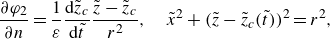 \begin{align}& \frac {\partial \varphi _2}{\partial n}=\frac {1}{\varepsilon }\frac {{\rm d}{\tilde {z}}_{c}}{{\rm d}\tilde {t}}\frac {{\tilde {z}}-{\tilde {z}}_{c}}{r^2},\quad \tilde {x}^2+({\tilde {z}}-{\tilde {z}}_{c}(\tilde {t}))^2=r^2, \end{align}
 \begin{align}&\qquad\quad\qquad |\nabla \varphi _2|\to 0,\quad {\tilde {z}}\to -\infty .\end{align}
The continuity of the vertical velocity and of the pressure at the interface connects the interface location $\tilde {\eta }$
with the potentials:
$\tilde {\eta }$
with the potentials:
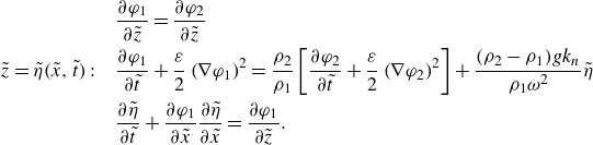 \begin{align} &\frac {\partial \varphi _1}{\partial {\tilde {z}}}=\frac {\partial \varphi _2}{\partial {\tilde {z}}}\notag\\{\tilde {z}}=\tilde {\eta }(\tilde {x},\tilde {t}):\quad &\frac {\partial \varphi _1}{\partial \tilde {t}}+\frac {\varepsilon }{2}\left (\nabla \varphi _1\right )^2=\frac {\rho _2}{\rho _1}\left [\frac {\partial \varphi _2}{\partial \tilde {t}}+\frac {\varepsilon }{2}\left (\nabla \varphi _2\right )^2\right ]+\frac {(\rho _2-\rho _1)gk_n}{\rho _1\omega ^2}\tilde {\eta } \notag\\ &\frac {\partial \tilde {\eta }}{\partial \tilde {t}}+\frac {\partial \varphi _1}{\partial \tilde {x}}\frac {\partial \tilde {\eta }}{\partial \tilde {x}}=\frac {\partial \varphi _1}{\partial {\tilde {z}}}. \end{align}
Neglecting terms of the order of $(\rho _2-\rho _1)/\rho _1$
and
$(\rho _2-\rho _1)/\rho _1$
and $\varepsilon$
and eliminating
$\varepsilon$
and eliminating $\eta$
yields a simplified linear problem for potentials:
$\eta$
yields a simplified linear problem for potentials:
 \begin{align} &\qquad\qquad\nabla ^2\varphi _1=0,\quad -\pi \lt \tilde {x}\lt (n-1)\pi, \quad {\tilde {z}}\gt 0, \end{align}
 \begin{align} &\nabla ^2\varphi _2=0,\quad -\pi \lt \tilde {x}\lt (n-1)\pi, \quad {\tilde {z}}\lt 0,\quad \tilde {x}^2+({\tilde {z}}+h)^2\gt r^2, \end{align}
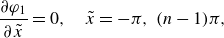 \begin{align} &\qquad\qquad\qquad\frac {\partial \varphi _1}{\partial \tilde {x}}=0,\quad \tilde {x}=-\pi, \ (n-1)\pi, \end{align}
 \begin{align} &\qquad\qquad\qquad\qquad|\nabla \varphi _1|\to 0,\quad {\tilde {z}}\to \infty, \end{align}
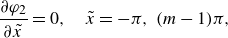 \begin{align} &\qquad\qquad\qquad\frac {\partial \varphi _2}{\partial \tilde {x}}=0,\quad \tilde {x}=-\pi, \ (m-1)\pi, \end{align}
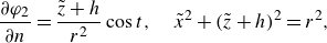 \begin{align} &\qquad\qquad\frac {\partial \varphi _2}{\partial n}=\frac {{\tilde {z}}+h}{r^2}\cos t,\quad \tilde {x}^2+({\tilde {z}}+h)^2=r^2, \end{align}
 \begin{align} &\qquad\qquad\qquad\quad|\nabla \varphi _2|\to 0,\quad {\tilde {z}}\to -\infty, \end{align}
 \begin{align} &\qquad\qquad\qquad\qquad\frac {\partial \varphi _1}{\partial {\tilde {z}}}=\frac {\partial \varphi _2}{\partial {\tilde {z}}},\quad {\tilde {z}}=0, \end{align}
 \begin{align} &\qquad\qquad\quad\frac {\partial ^{2} \varphi _1}{\partial \tilde {t}^2}=\frac {\partial ^2 \varphi _2}{\partial \tilde {t}^2}+\frac {2}{\alpha ^2}\frac {\partial \varphi _2}{\partial {\tilde {z}}},\quad {\tilde {z}}=0. \end{align}
The violation of the symmetry between the upper and the lower liquids is due to the presence of the wavemaker under the interface. It leads to the failure of the solution of Lamb (Reference Lamb1932) as it does not satisfy the boundary condition at the wavemaker (4.8f ). The Lamb solution in the upper liquid is retained:
 \begin{equation} \varphi _1=\sum \limits _{m=1}^\infty a_m\varphi _{1,m},\quad \varphi _{1,m}=\frac {1}{2}\left [\cos \left (\frac {m}{n}(\tilde {x}+\pi )\right )\exp \left (-\frac {m}{n}{\tilde {z}}\right )\exp (-i\tilde {t})+\text{c.c.}\right ]. \end{equation}
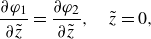
In the lower liquid, the solution is represented as a superposition of the forcing potential $\varphi _0$
and wavemodes
$\varphi _0$
and wavemodes $\varphi _{2,m}$
:
$\varphi _{2,m}$
:
 \begin{equation} \varphi _2=\varphi _0+\sum \limits _{m=1}^\infty b_m\varphi _{2,m}. \end{equation}
The potential $\varphi _0$
satisfies equation (4.8b
) with boundary conditions (4.8e
–g
), including the inhomogeneous boundary condition (4.8f
). The potentials
$\varphi _0$
satisfies equation (4.8b
) with boundary conditions (4.8e
–g
), including the inhomogeneous boundary condition (4.8f
). The potentials $\varphi _{2,m}$
satisfy the homogeneous boundary condition at the wavemaker:
$\varphi _{2,m}$
satisfy the homogeneous boundary condition at the wavemaker:
 \begin{align}&\qquad\qquad\qquad\qquad \frac {\partial \varphi _{2,m}}{\partial n}=0,\quad \tilde {x}^2+({\tilde {z}}+h)^2=r^2\nonumber\\& \varphi _{2,m}=\frac {1}{2}\left \{\left [\cos \left (\frac {m}{n}(\tilde {x}+\pi )\right )\exp \left (\frac {m}{n}{\tilde {z}}\right )+\varphi _{2,m}^{\prime}\right ]\exp (-i\tilde {t})+\text{c.c.} \right \} .\end{align}
The symmetry of the functions $\varphi _0$
and
$\varphi _0$
and $\varphi _{2,m}^{\prime}$
with respect to
$\varphi _{2,m}^{\prime}$
with respect to ${\tilde {z}}=-h$
is also required for uniqueness; they are represented by series of multipoles placed at the wavemaker centre and their successive mirror reflections with respect to the basin walls (Mogilevskiy et al. Reference Mogilevskiy, Kalenko, Zemach and Shemer2024). The leading terms are
${\tilde {z}}=-h$
is also required for uniqueness; they are represented by series of multipoles placed at the wavemaker centre and their successive mirror reflections with respect to the basin walls (Mogilevskiy et al. Reference Mogilevskiy, Kalenko, Zemach and Shemer2024). The leading terms are
 \begin{align} &\,\,\, \varphi _0=\frac {1}{2}\left [-\frac {r^2(z+h)}{x^2+(z+h)^2}\exp (-i\tilde {t})+\text{c.c.}\right ];\nonumber\\& \varphi _{2,m}^{\prime}=\frac {1}{2}\left [-\frac {m}{n}\exp \left (-\frac {m}{n}h\right )\frac {r^2(z+h)}{x^2+(z+h)^2}\right ]. \end{align}
The forcing potential $\varphi _0$
introduces disturbances of the order of
$\varphi _0$
introduces disturbances of the order of $r^2/h$
to all spatial modes (figure 11); the wavenumber spectrum has peaks at
$r^2/h$
to all spatial modes (figure 11); the wavenumber spectrum has peaks at $m=n,\ 2n, \ldots$
, since the wavemaker is located at the antinode of those modes. The response of the system is defined by the boundary conditions (4.8h
) and (4.8i
) representing the continuity of the vertical velocity and the pressure at the interface. The substitution of (4.9), (4.10) yields the system of linear algebraic equations for
$m=n,\ 2n, \ldots$
, since the wavemaker is located at the antinode of those modes. The response of the system is defined by the boundary conditions (4.8h
) and (4.8i
) representing the continuity of the vertical velocity and the pressure at the interface. The substitution of (4.9), (4.10) yields the system of linear algebraic equations for $a_m$
and
$a_m$
and $b_m$
:
$b_m$
:
 \begin{equation} \begin{array}{c} \displaystyle { \int \limits _{-\pi }^{(n-1)\pi }\left [ \sum \limits _{m=1}^\infty a_m\frac {\partial \varphi _{1,m}(\tilde {x},0)}{\partial {\tilde {z}}}-\sum \limits _{m=1}^\infty b_m\frac {\partial \varphi _{2,m}(\tilde {x},0)}{\partial {\tilde {z}}}\right .}\\ \displaystyle {\left . -\frac {\partial \varphi _0(\tilde {x},0)}{\partial {\tilde {z}}} \right ]\cos \left (\frac {l}{n}(\tilde {x}+\pi )\right ){\rm d}\tilde {x}=0},\\ \displaystyle { \int \limits _{-\pi }^{(n-1)\pi }\left \{ \sum \limits _{m=1}^\infty a_m\varphi _{1,m}(\tilde {x},0)-\sum \limits _{m=1}^\infty b_m\left [\varphi _{2,m}(\tilde {x},0)-\frac {2}{\alpha ^2}\frac {\partial \varphi _{2,m}(\tilde {x},0)}{\partial {\tilde {z}}}\right ]\right .}\\ \displaystyle {-\left .\left [\varphi _{0}(\tilde {x},0)-\frac {2}{\alpha ^2}\frac {\partial \varphi _{0}(\tilde {x},0)}{\partial {\tilde {z}}}\right ] \right \}\cos \left (\frac {l}{n}(\tilde {x}+\pi )\right )d\tilde {x}=0},\\ l=1\ldots \infty .\end{array} \end{equation}
The free terms associated with $\varphi _0$
are of the order of
$\varphi _0$
are of the order of $r^2/h$
(see (4.12)). It can be shown that the eigenvalue of the system (4.13) is
$r^2/h$
(see (4.12)). It can be shown that the eigenvalue of the system (4.13) is $\alpha =m/n-\Delta \alpha _m$
, where
$\alpha =m/n-\Delta \alpha _m$
, where $0\lt \Delta \alpha _m\sim r^2/(\pi n h)$
corresponds to the downshift of the resonant frequency due to the finite wavemaker size. For other values of
$0\lt \Delta \alpha _m\sim r^2/(\pi n h)$
corresponds to the downshift of the resonant frequency due to the finite wavemaker size. For other values of $\alpha$
, (4.13) has a unique solution.
$\alpha$
, (4.13) has a unique solution.
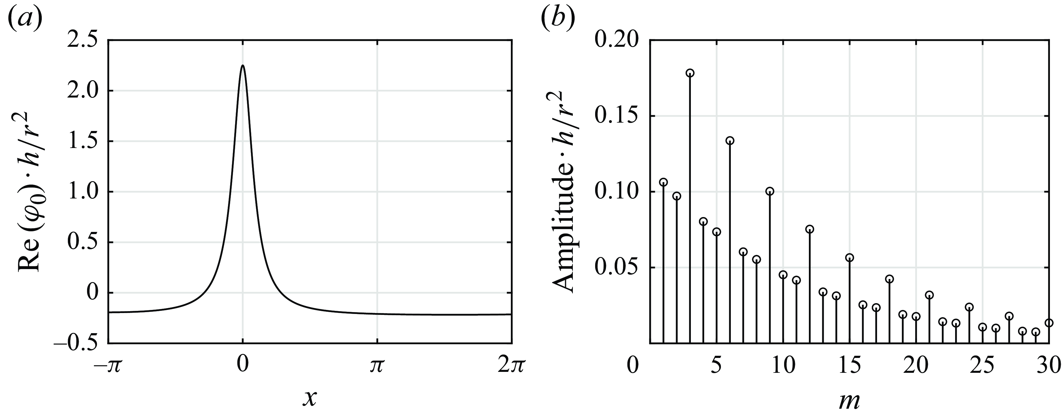
Figure 11. (a) Normalised forcing potential at ${\tilde {z}}=0$
and (b) its wavenumber amplitude spectrum.
${\tilde {z}}=0$
and (b) its wavenumber amplitude spectrum.
This simplified two-layer model demonstrates the general approach; however, the predicted downshift of the resonant frequency from $\alpha =1$
is about 1 %, an order of magnitude smaller than that measured in experiments (§ 3). The experimental results plotted in figure 10 indicate the significant effect of the thickness of the pycnocline, which is neglected in the two-layer model.
$\alpha =1$
is about 1 %, an order of magnitude smaller than that measured in experiments (§ 3). The experimental results plotted in figure 10 indicate the significant effect of the thickness of the pycnocline, which is neglected in the two-layer model.
4.2. Eigenfunctions for continuous stratification
In the linear approximation, the complex amplitude function for the vertical velocity $W_m({\tilde {z}})$
for a wave with the wavemode number
$W_m({\tilde {z}})$
for a wave with the wavemode number $m$
satisfies the Taylor–Goldstein equation (Goldstein Reference Goldstein1931; Taylor Reference Taylor1931) for a given dimensionless buoyancy frequency distribution
$m$
satisfies the Taylor–Goldstein equation (Goldstein Reference Goldstein1931; Taylor Reference Taylor1931) for a given dimensionless buoyancy frequency distribution ${\tilde {N}}({\tilde {z}}$
):
${\tilde {N}}({\tilde {z}}$
):
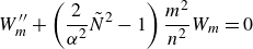 \begin{equation} W_m^{\prime\prime}+\left (\frac {2}{\alpha ^2}{\tilde {N}}^2-1\right )\frac {m^2}{n^2}W_m=0 \end{equation}
and the boundary conditions
 \begin{equation} W_m\to 0,\quad {\tilde {z}}\to \pm \infty, \end{equation}
where primes denote derivatives with respect to $\tilde {z}$
. The analysis of this Sturm–Liouville problem shows that for any given
$\tilde {z}$
. The analysis of this Sturm–Liouville problem shows that for any given $m$
, there is an infinite number of solutions
$m$
, there is an infinite number of solutions $W_m^{j}$
and corresponding
$W_m^{j}$
and corresponding $\alpha _{m,j}$
that are orthogonal with the weight function
$\alpha _{m,j}$
that are orthogonal with the weight function ${\tilde {N}}^2$
(Morse & Feshbach Reference Morse and Feshbach1946):
${\tilde {N}}^2$
(Morse & Feshbach Reference Morse and Feshbach1946):
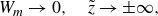
 \begin{equation} \int \limits _{-\infty }^\infty W_m^{j1}W_m^{j2}{\tilde {N}}^2{\rm d}{\tilde {z}}=0,\quad j_1\neq j_2. \end{equation}
For the piecewise-constant distribution ${\tilde {N}}^2({\tilde {z}})$
:
${\tilde {N}}^2({\tilde {z}})$
:
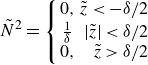 \begin{equation} {\tilde {N}}^2=\left \{ \begin{array}{cr} 0,& {\tilde {z}}\lt -\delta /2\\ \frac {1}{\delta}& |{\tilde {z}}|\lt \delta /2\\ 0,& {\tilde {z}}\gt \delta /2 \end{array} \right . \end{equation}
the analytical solution for $W_{m}^j$
is
$W_{m}^j$
is
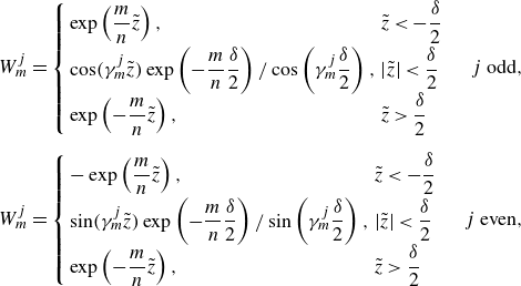 \begin{equation} \begin{array}{c} W_{m}^{j}=\left \{ \begin{array}{ll} \exp \left (\dfrac {m}{n}{\tilde {z}}\right ),& {\tilde {z}}\lt -\dfrac {\delta }{2}\\[6pt] \cos (\gamma _{m}^{j} {\tilde {z}})\exp \left (-\dfrac {m}{n}\dfrac {\delta }{2}\right )/\cos \left (\gamma _{m}^{j}\dfrac {\delta }{2} \right ),& |{\tilde {z}}|\lt \dfrac {\delta }{2}\\[6pt] \exp \left (-\dfrac {m}{n}{\tilde {z}}\right ),& {\tilde {z}}\gt \dfrac {\delta }{2} \end{array} \right . \quad j \text{ odd},\\ \\[-2pt] W_{m}^{j}=\left \{ \begin{array}{ll} -\exp \left (\dfrac {m}{n}{\tilde {z}}\right ),& {\tilde {z}}\lt -\dfrac {\delta }{2}\\[6pt] \sin (\gamma _{m}^{j} {\tilde {z}})\exp \left (-\dfrac {m}{n}\dfrac {\delta }{2}\right )/\sin \left (\gamma _{m}^{j}\dfrac {\delta }{2} \right ),& |{\tilde {z}}|\lt \dfrac {\delta }{2}\\[6pt] \exp \left (-\dfrac {m}{n}{\tilde {z}}\right ),& {\tilde {z}}\gt \dfrac {\delta }{2} \end{array} \right .\quad j \text{ even},\\ \end{array} \end{equation}
where
 \begin{equation} \left (\gamma _{m}^{j}\right )^2=\left (\frac {2}{\left (\alpha _{m}^{j}\right )^2\delta }-1\right )\frac {m^2}{n^2} \end{equation}
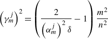
are roots of one of the equations:
 \begin{align} &\,\gamma \tan \frac {\gamma \delta }{2}=\frac {m}{n}, \end{align}
 \begin{align} &\gamma \cot \frac {\gamma \delta }{2}=-\frac {m}{n} \end{align}
(Miropol’sky & Shishkina Reference Miropol’sky and Shishkina2001). Equations (4.20a
) and (4.20b
) correspond to the eigenvalues with odd and even superscript indices. The function $W_{m}^j$
has
$W_{m}^j$
has $j-1$
zeros within the pycnocline; it is symmetric for odd
$j-1$
zeros within the pycnocline; it is symmetric for odd $j$
and antisymmetric for even
$j$
and antisymmetric for even $j$
with respect to
$j$
with respect to ${\tilde {z}}=0$
. The resonant mode in the two-layer model corresponds to
${\tilde {z}}=0$
. The resonant mode in the two-layer model corresponds to $\alpha _*=\alpha _{n}^1$
, in the limit
$\alpha _*=\alpha _{n}^1$
, in the limit $\delta \ll 1$
,
$\delta \ll 1$
,
 \begin{equation} \alpha _*=1-\frac {\delta }{6}+O(\delta ^2) \end{equation}
(Thorpe Reference Thorpe1968). Figure 12 presents the eigenfrequencies $\alpha _m^j$
as well as the eigenfunctions
$\alpha _m^j$
as well as the eigenfunctions $W_m^j$
for
$W_m^j$
for $j=1,\ 2$
. Note that
$j=1,\ 2$
. Note that $W_m^{1}$
tends to the Lamb solution as
$W_m^{1}$
tends to the Lamb solution as $\delta \to 0$
. For finite
$\delta \to 0$
. For finite $\delta$
, the eigenfrequency is downshifted from that of the Lamb solution by 6–10 % in the present experiments.
$\delta$
, the eigenfrequency is downshifted from that of the Lamb solution by 6–10 % in the present experiments.
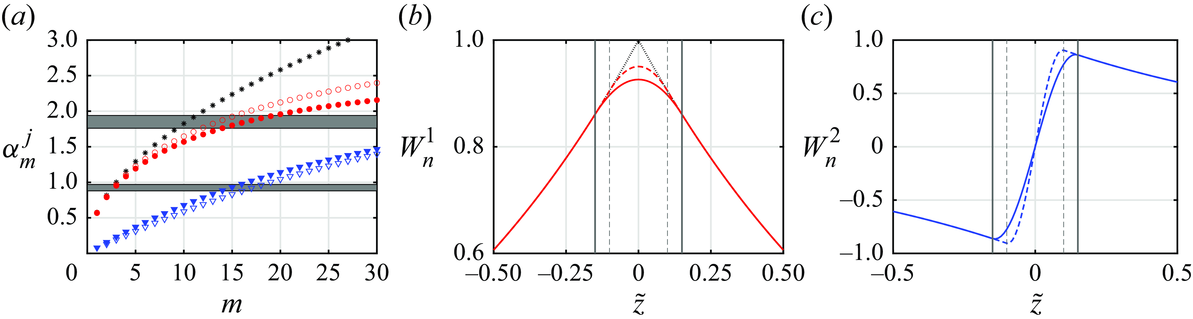
Figure 12. (a) Eigenfrequencies of the first symmetric ( $j=1$
, red) and antisymmetric (
$j=1$
, red) and antisymmetric ( $j=2$
, blue) modes for
$j=2$
, blue) modes for $\delta =0.2$
(open symbols) and
$\delta =0.2$
(open symbols) and $\delta =0.3$
(filled symbols); asterisks represent the two-layer model. The corresponding eigenfunctions
$\delta =0.3$
(filled symbols); asterisks represent the two-layer model. The corresponding eigenfunctions $W_n^1$
(b) and
$W_n^1$
(b) and $W_n^2$
(c) for
$W_n^2$
(c) for $\delta =0.2$
(solid lines) and
$\delta =0.2$
(solid lines) and $\delta =0.3$
(dashed lines). The experimental ranges of the forcing frequency and its second harmonic are shaded in (a), the dotted line in (b) represents the eigenfunction for the two-layer model and the vertical lines in (b,c) show the boundaries of the pycnocline.
$\delta =0.3$
(dashed lines). The experimental ranges of the forcing frequency and its second harmonic are shaded in (a), the dotted line in (b) represents the eigenfunction for the two-layer model and the vertical lines in (b,c) show the boundaries of the pycnocline.
4.3. Linear model for finite pycnocline thickness
The solution procedure follows the two-layer model approach. In this subsection, the simplified form of the potential solution (4.10) in the lower liquid ( ${\tilde {z}}\lt -\delta /2$
) is used, neglecting terms
${\tilde {z}}\lt -\delta /2$
) is used, neglecting terms $\varphi _{2,m}^{\prime}$
in (4.11) associated with the finite wavemaker size:
$\varphi _{2,m}^{\prime}$
in (4.11) associated with the finite wavemaker size:
 \begin{equation} \varphi _2=\varphi _0+\frac {1}{2}\left [\sum \limits _{m=1}^\infty b_m\cos \left (\frac {m}{n}(\tilde {x}+\pi )\right )\exp \left (\frac {m}{n}{\tilde {z}}\right )\exp (-i\tilde {t})+\text{ c.c.}\right ]. \end{equation}
The vertical velocity in the upper liquid, including the pycnocline, is the solution of the Taylor–Goldstein equation (4.14):
 \begin{equation} w=\frac {1}{2}\left [\sum \limits _{m=1}^\infty a_m W_m({\tilde {z}})\cos \left (\frac {m}{n}(\tilde {x}+\pi )\right )\exp (-i\tilde {t})+\text{ c.c.}\right ]; \quad W_m\to 0,\ {\tilde {z}}\to \infty . \end{equation}
Equation (4.14) is also valid in the lower liquid, so the solution can be smoothly extended to ${\tilde {z}}\lt -\delta /2$
:
${\tilde {z}}\lt -\delta /2$
:
 \begin{align} W_m=\left \{ \begin{array}{ll} C_1^{m}\exp \left(\dfrac {m}{n}{\tilde {z}}\right)+C_2^{m}\exp \left(-\dfrac {m}{n}{\tilde {z}}\right)&{\tilde {z}}\lt -\delta /2\\[7pt] C_3^{m}\cos (\gamma {\tilde {z}})+C_4^{m}\sin (\gamma {\tilde {z}})&|{\tilde {z}}|\lt \delta /2\\[7pt] \exp \left(-\dfrac {m}{n}{\tilde {z}}\right)&{\tilde {z}}\gt \delta /2 \end{array} \right . \quad \gamma ^2=\left (\dfrac {2}{\alpha ^2\delta }-1\right )\dfrac {m^2}{n^2}. \end{align}
The constants $C_1^{m},\ldots, C_4^{m}$
are found from the continuity conditions of
$C_1^{m},\ldots, C_4^{m}$
are found from the continuity conditions of $W_m$
and
$W_m$
and $W_m^{\prime}$
at
$W_m^{\prime}$
at ${\tilde {z}}=\pm \delta /2$
; the coefficient at the exponent for
${\tilde {z}}=\pm \delta /2$
; the coefficient at the exponent for ${\tilde {z}}\gt \delta \gt /2$
is chosen as unity for normalisation. For frequencies different from the eigenvalues
${\tilde {z}}\gt \delta \gt /2$
is chosen as unity for normalisation. For frequencies different from the eigenvalues $\alpha \neq \alpha _{m}^j$
, the solution is unbounded as
$\alpha \neq \alpha _{m}^j$
, the solution is unbounded as $z\to -\infty$
(
$z\to -\infty$
( $C_2^{m}\neq 0$
). Examples of functions
$C_2^{m}\neq 0$
). Examples of functions $W_n$
are shown in figure 13(a).
$W_n$
are shown in figure 13(a).
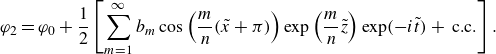
Figure 13. (a) The vertical velocity profiles $W_n$
in the upper liquid extended to
$W_n$
in the upper liquid extended to ${\tilde {z}}\lt -\delta /2$
. (b) The sum of
${\tilde {z}}\lt -\delta /2$
. (b) The sum of $ {{\rm d}\varPhi _n}/{{\rm d}{\tilde {z}}}$
(in black) and
$ {{\rm d}\varPhi _n}/{{\rm d}{\tilde {z}}}$
(in black) and $b_n\exp ({\tilde {z}})$
(in blue) matches
$b_n\exp ({\tilde {z}})$
(in blue) matches $a_nW_n$
(in red); the coefficients are defined by (4.26). Thin vertical lines denote the boundaries of the pycnocline;
$a_nW_n$
(in red); the coefficients are defined by (4.26). Thin vertical lines denote the boundaries of the pycnocline; $\delta =0.2$
,
$\delta =0.2$
, $\alpha =\alpha _*+0.1$
.
$\alpha =\alpha _*+0.1$
.
Following Morse & Feshbach (Reference Morse and Feshbach1946), the contributions of the forcing potential $\varphi _0$
to the
$\varphi _0$
to the $m$
th spatial mode in the region between the wavemaker top and the lower boundary of the pycnocline
$m$
th spatial mode in the region between the wavemaker top and the lower boundary of the pycnocline $-h+r\lt {\tilde {z}}\lt -\delta /2$
can be represented as
$-h+r\lt {\tilde {z}}\lt -\delta /2$
can be represented as
 \begin{align} \varPhi _m=\int \limits _{-\pi }^{(n-1)\pi }\varphi _0(\tilde {x},{\tilde {z}})\cos \left (\frac {m}{n}(\tilde {x}+\pi )\right ){\rm d}\tilde {x}=Q_1^{m}\exp \left (\frac {m}{n}{\tilde {z}}\right )+Q_2^{m}\exp \left (-\frac {m}{n}{\tilde {z}}\right ). \end{align}
The conditions
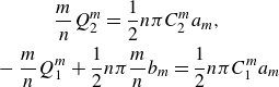 \begin{align} &\qquad\quad\frac {m}{n}Q_2^{m}=\frac {1}{2}n\pi C_2^{m} a_m,\nonumber\\& -\frac {m}{n}Q_1^{m}+\frac {1}{2}n\pi \frac {m}{n}b_m=\frac {1}{2}n\pi C_1^{m} a_m \end{align}
ensure matching of both vertical and horizontal velocities defined by (4.22) and (4.23) at the vertical locations $-h+r\lt {\tilde {z}}\lt -\delta /2$
(figure 13
b). The amplitudes
$-h+r\lt {\tilde {z}}\lt -\delta /2$
(figure 13
b). The amplitudes $A_w^m$
and
$A_w^m$
and $A_u^m$
of the vertical and horizontal velocity components for the
$A_u^m$
of the vertical and horizontal velocity components for the $m$
th mode are
$m$
th mode are
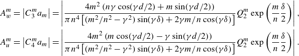 \begin{align} &A_w^m=\left |C_3^{m}a_m\right |=\left |\frac {4 m^2\left (n\gamma \cos (\gamma d/2)+m\sin (\gamma d/2)\right )}{\pi n^4\left [(m^2/n^2-\gamma ^2) \sin (\gamma \delta )+2\gamma m/n\cos (\gamma \delta )\right ] }Q_2^{m}\exp \left (\frac {m}{n}\frac {\delta }{2}\right )\right |,\notag\\ & A_u^m=\left |C_4^{m}a_m\right |=\left |\frac {4 m^2\left (m\cos (\gamma d/2)-\gamma \sin (\gamma d/2)\right )}{\pi n^4\left [(m^2/n^2-\gamma ^2) \sin (\gamma \delta )+2\gamma m/n\cos (\gamma \delta )\right ] }Q_2^{m}\exp \left (\frac {m}{n}\frac {\delta }{2}\right )\right |. \end{align}
The singularity leading to infinite velocity amplitude appears if (4.20a
) or (4.20b
) is satisfied. The amplitude of the vertical velocity at the antinode $(\tilde {x},{\tilde {z}})=(\pi, 0)$
is dominated by the contribution of the
$(\tilde {x},{\tilde {z}})=(\pi, 0)$
is dominated by the contribution of the $n$
th mode, provided
$n$
th mode, provided $\alpha$
is close to
$\alpha$
is close to $\alpha _*$
:
$\alpha _*$
:
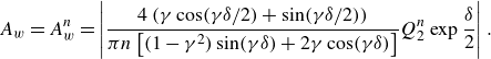 \begin{align} A_w=A_w^n=\left |\frac {4 \left (\gamma \cos (\gamma \delta /2)+\sin (\gamma \delta /2)\right )}{\pi n\left [(1-\gamma ^2) \sin (\gamma \delta )+2\gamma \cos (\gamma \delta )\right ] }Q_2^{n}\exp \frac {\delta }{2}\right |. \end{align}
The amplitude is inversely proportional to the detuning $\beta$
:
$\beta$
:
 \begin{equation} \beta =\alpha -\alpha _*, \end{equation}
since $(A_w)^{-1}=0$
for
$(A_w)^{-1}=0$
for $\beta =0$
. The Taylor expansion in the vicinity of
$\beta =0$
. The Taylor expansion in the vicinity of $\beta =0$
yields
$\beta =0$
yields
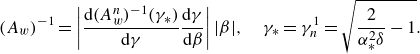 \begin{align} (A_w)^{-1}=\left |\frac {{\rm d}(A_w^n)^{-1}(\gamma _*)}{{\rm d}\gamma }\frac {{\rm d}\gamma }{{\rm d}\beta }\right | |\beta |,\quad \gamma _*=\gamma _n^1=\sqrt {\frac {2}{\alpha _*^2\delta }-1}. \end{align}
The slope of the linear dependence of the inverse amplitude on the detuning depends only on $\delta$
, since
$\delta$
, since $\gamma _*$
and the corresponding eigenfrequency
$\gamma _*$
and the corresponding eigenfrequency $\alpha _*$
are given by (4.20a
) and (4.19), respectively. Calculations show that this slope varies within 5 % for
$\alpha _*$
are given by (4.20a
) and (4.19), respectively. Calculations show that this slope varies within 5 % for $0\lt \delta \lt 1$
. The limit for
$0\lt \delta \lt 1$
. The limit for $\delta \to 0$
is
$\delta \to 0$
is
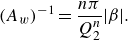 \begin{equation} (A_w)^{-1}=\frac {n\pi }{Q_2^{n}} |\beta |. \end{equation}
4.4. Effect of dissipation
Accounting for the dissipation due to the friction at the front and back walls of the basin within the Stokes layer model can be performed similarly, since the corresponding generalisation of the Taylor–Goldstein equation (4.14) retains a similar form (see Appendix A for details):
 \begin{align} & W_m^{\prime\prime}+\left (\frac {2}{\alpha ^2 (1+s)}{\tilde {N}}^2-1\right )\frac {m^2}{n^2}W_m=0,\notag\\ &\qquad s=\sqrt {2}(1+i)\sqrt {\frac {\mu }{\rho _0 B^2}}\sim 10^{-2}, \end{align}
where $\mu$
is the dynamic viscosity. The form (4.14) is obtained from (4.32) defining the effective detuning as
$\mu$
is the dynamic viscosity. The form (4.14) is obtained from (4.32) defining the effective detuning as
 \begin{align} \beta '=\beta +\frac {s\alpha _*}{2}. \end{align}
Equation (4.31) shows that the maximum amplitude is inversely proportional to $|s|$
and corresponds to
$|s|$
and corresponds to $\beta =-\alpha _*\textrm {Re}(s)/2\lt 0$
. The Stokes layer dissipation model does not account for viscous interaction between the wavemaker and the liquid; thus, for comparison with the experiments,
$\beta =-\alpha _*\textrm {Re}(s)/2\lt 0$
. The Stokes layer dissipation model does not account for viscous interaction between the wavemaker and the liquid; thus, for comparison with the experiments, $s$
can be treated as a free parameter of the order of
$s$
can be treated as a free parameter of the order of $10^{-2}$
.
$10^{-2}$
.
The dissipation in bulk is more significant for the shorter waves. The solution in the upper liquid is governed by the fourth-order equation (see Appendix A for details)
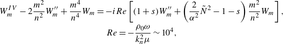 \begin{align} & W_m^{IV}-2\frac {m^2}{n^2}W_m^{\prime\prime}+\frac {m^4}{n^4}W_m=-i{Re}\left [(1+s)W_m^{\prime\prime}+\left (\frac {2}{\alpha ^2 }{\tilde {N}}^2 -1 -s\right )\frac {m^2}{n^2}W_m\right ],\notag\\&\qquad\qquad\qquad\qquad\qquad\qquad {Re}=-\frac {\rho _0\omega }{k_n^2\mu }\sim 10^4, \end{align}
with boundary conditions
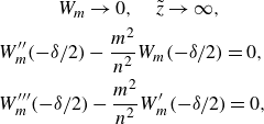 \begin{align} &\qquad\quad W_m\to 0, \quad {\tilde {z}}\to \infty, \notag\\& W_{m}^{\prime\prime}(-\delta /2)-\frac {m^2}{n^2}W_m(-\delta /2)=0,\notag\\ & W_{m}^{\prime\prime\prime}(-\delta /2)-\frac {m^2}{n^2}W_{m}^{\prime}(-\delta /2)=0, \end{align}
that ensure vanishing of the velocity amplitude at infinity and matching to the potential solution in the lower liquid. The solution for $W_m$
is found numerically, then smoothly extended to the region
$W_m$
is found numerically, then smoothly extended to the region ${\tilde {z}}\lt -\delta /2$
. The above-described matching procedure is then applied.
${\tilde {z}}\lt -\delta /2$
. The above-described matching procedure is then applied.
Correction to the eigenfunctions $\varphi _{2,m}$
to account for the finite wavemaker size by imposing boundary conditions (4.11) does not change the procedure significantly. The contribution of the eigenfunctions to the
$\varphi _{2,m}$
to account for the finite wavemaker size by imposing boundary conditions (4.11) does not change the procedure significantly. The contribution of the eigenfunctions to the $m$
th spatial mode is a sum of
$m$
th spatial mode is a sum of $\exp (m{\tilde {z}}/n)$
and
$\exp (m{\tilde {z}}/n)$
and $\exp (-m{\tilde {z}}/n)$
. Matching of the vertical velocity and its
$\exp (-m{\tilde {z}}/n)$
. Matching of the vertical velocity and its $\tilde {z}$
derivative at any point
$\tilde {z}$
derivative at any point ${\tilde {z}}_c\in (-h+r,-\delta /2)$
ensures the matching of the solutions in the entire region
${\tilde {z}}_c\in (-h+r,-\delta /2)$
ensures the matching of the solutions in the entire region $-h+r\lt {\tilde {z}}\lt -\delta /2$
. The coefficients
$-h+r\lt {\tilde {z}}\lt -\delta /2$
. The coefficients $a_m$
and
$a_m$
and $b_m$
in the decompositions (4.23) and (4.10) are found from the system of equations
$b_m$
in the decompositions (4.23) and (4.10) are found from the system of equations
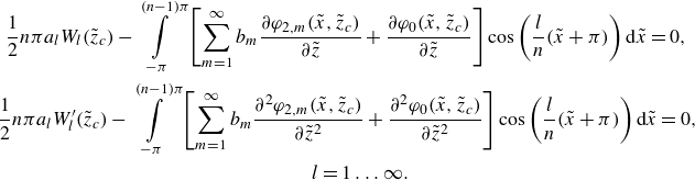 \begin{align} &\,\, \frac {1}{2}n\pi a_lW_l({\tilde {z}}_c)-\int \limits _{-\pi }^{(n-1)\pi }\left [\sum \limits _{m=1}^\infty b_m\frac {\partial \varphi _{2,m}(\tilde {x},{\tilde {z}}_c)}{\partial {\tilde {z}}} +\frac {\partial \varphi _0(\tilde {x},{\tilde {z}}_c)}{\partial {\tilde {z}}} \right ]\cos \left (\frac {l}{n}(\tilde {x}+\pi )\right ){\rm d}\tilde {x}=0,\notag\\& \frac {1}{2}n\pi a_lW_l^{\prime}({\tilde {z}}_c)-\int \limits _{-\pi }^{(n-1)\pi }\left [ \sum \limits _{m=1}^\infty b_m\frac {\partial ^2 \varphi _{2,m}(\tilde {x},{\tilde {z}}_c)}{\partial \tilde {z}^2}+\frac {\partial ^2 \varphi _{0}(\tilde {x},{\tilde {z}}_c)}{\partial \tilde {z}^2} \right ]\cos \left (\frac {l}{n}(\tilde {x}+\pi )\right ){\rm d}\tilde {x}=0,\notag\\ &\qquad\qquad\qquad\qquad\qquad\qquad\qquad\qquad l=1\ldots \infty . \end{align}
For arbitrary density gradient distribution ${\tilde {N}}({\tilde {z}})$
, a boundary
${\tilde {N}}({\tilde {z}})$
, a boundary ${\tilde {z}}_*$
is selected so that
${\tilde {z}}_*$
is selected so that ${\tilde {N}}({\tilde {z}})\ll 1$
for
${\tilde {N}}({\tilde {z}})\ll 1$
for ${\tilde {z}}\lt {\tilde {z}}_*$
. The boundary conditions (4.35) are set at
${\tilde {z}}\lt {\tilde {z}}_*$
. The boundary conditions (4.35) are set at ${\tilde {z}}_*$
, and the matching conditions (4.36) are also applied there. The analytical inviscid results for the piecewise-constant
${\tilde {z}}_*$
, and the matching conditions (4.36) are also applied there. The analytical inviscid results for the piecewise-constant ${\tilde {N}}({\tilde {z}})$
as well as the numerical computations based on the present model confirm that the results practically do not depend on the particular choice of
${\tilde {N}}({\tilde {z}})$
as well as the numerical computations based on the present model confirm that the results practically do not depend on the particular choice of ${\tilde {z}}_*$
.
${\tilde {z}}_*$
.
4.5. Numerical results
The numerical calculations are performed for the measured Gaussian buoyancy frequency distribution (2.5); the vertical velocity distribution is given by (4.23) and the corresponding horizontal velocity is
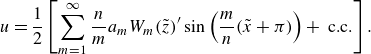 \begin{align} u=\frac {1}{2}\left [\sum \limits _{m=1}^\infty \frac {n}{m} a_m W_m({\tilde {z}})'\sin \left (\frac {m}{n}(\tilde {x}+\pi )\right )+\text{ c.c.}\right ]. \end{align}
Figure 14 shows an example of wavenumber amplitude spectra of vertical and horizontal velocities at ${\tilde {z}}=0$
accounting for the Stokes layer and both dissipation mechanisms discussed above. The wavenumber domains with dominant contributions to the vertical and the horizontal velocity components are clearly separated,
${\tilde {z}}=0$
accounting for the Stokes layer and both dissipation mechanisms discussed above. The wavenumber domains with dominant contributions to the vertical and the horizontal velocity components are clearly separated, $m=3$
and
$m=3$
and $m\approx 17$
, respectively, close to the wavenumbers that satisfy the dispersion relation for the symmetric and antisymmetric eigenfunctions. The effect of the bulk dissipation on the longer-mode amplitude is largely insignificant but is observed for the shorter modes. The dependence of the resonant amplitude modes on the detuning
$m\approx 17$
, respectively, close to the wavenumbers that satisfy the dispersion relation for the symmetric and antisymmetric eigenfunctions. The effect of the bulk dissipation on the longer-mode amplitude is largely insignificant but is observed for the shorter modes. The dependence of the resonant amplitude modes on the detuning $\beta$
agrees with the simplified model predictions (4.31) as confirmed by the comparison of the inverse amplitude values in figure 15.
$\beta$
agrees with the simplified model predictions (4.31) as confirmed by the comparison of the inverse amplitude values in figure 15.
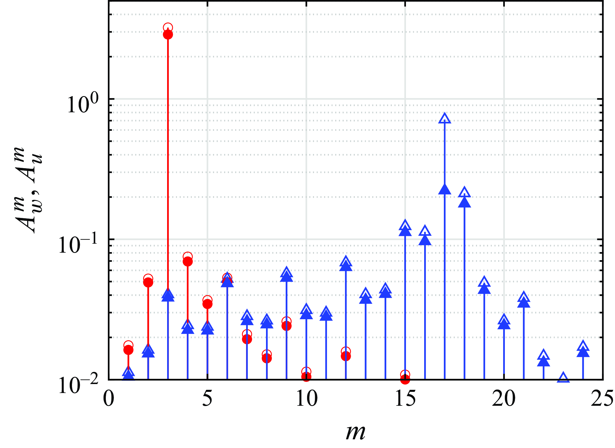
Figure 14. Wavenumber spectra of vertical (red) and horizontal (blue) velocity components at $z=0$
at an effective resonance
$z=0$
at an effective resonance $\alpha =0.94$
for
$\alpha =0.94$
for $\delta =0.24$
; open symbols account for dissipation in Stokes layers only, filled symbols for bulk dissipation as well.
$\delta =0.24$
; open symbols account for dissipation in Stokes layers only, filled symbols for bulk dissipation as well.
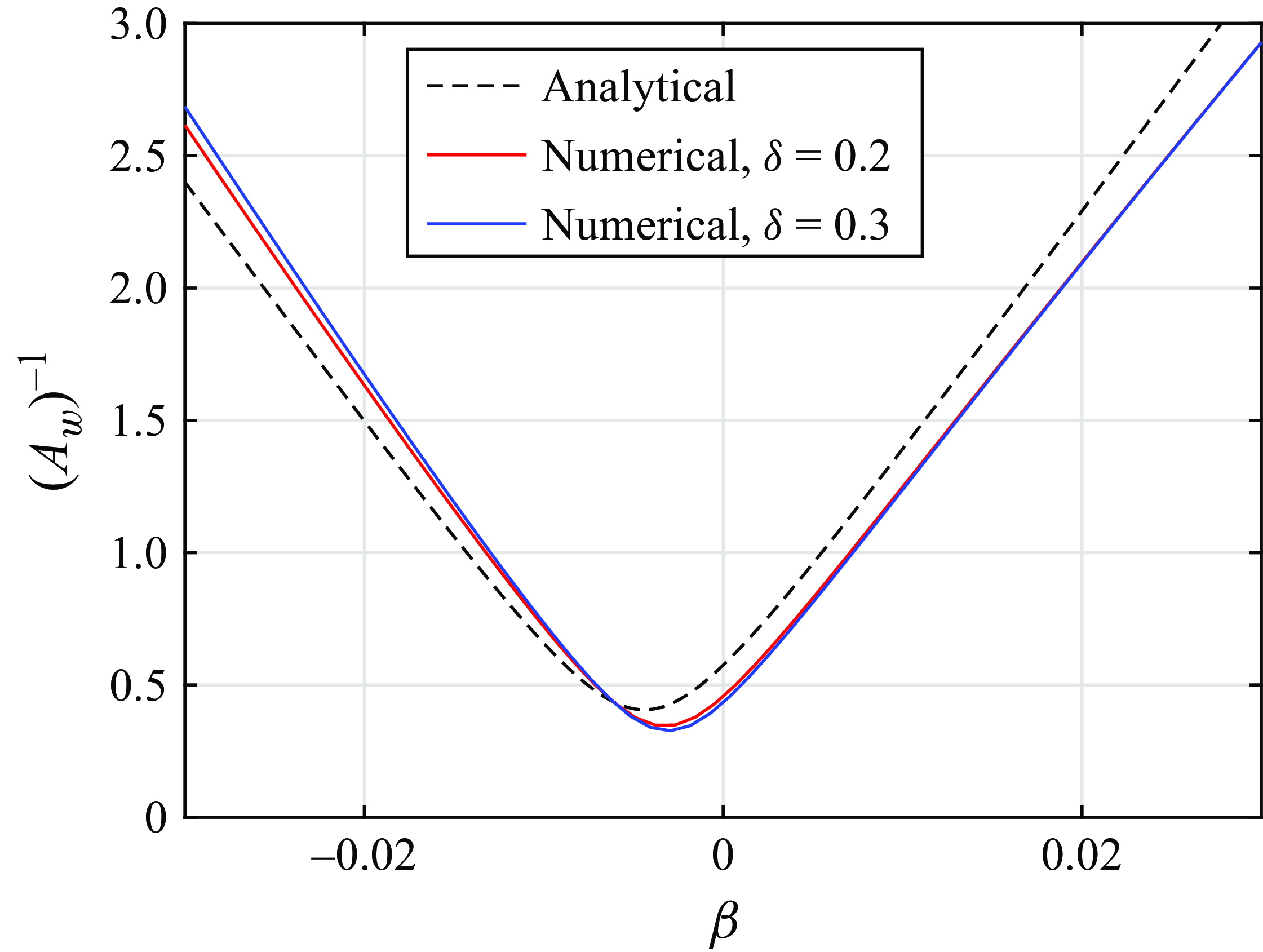
Figure 15. Inverse amplitude of the vertical velocity as a function of the detuning.
The amplitudes of the antisymmetric short modes with relatively large values of $m$
depend on the detuning
$m$
depend on the detuning $\beta$
in a complex way. Three modes with largest amplitudes are shown in figure 16 for two different pycnocline dimensionless thicknesses
$\beta$
in a complex way. Three modes with largest amplitudes are shown in figure 16 for two different pycnocline dimensionless thicknesses $\delta$
; the range of the corresponding values of
$\delta$
; the range of the corresponding values of $m$
shifts to the left as
$m$
shifts to the left as $\delta$
increases, in agreement with figure 12. For all modes in figure 16, a local amplitude maximum is located at
$\delta$
increases, in agreement with figure 12. For all modes in figure 16, a local amplitude maximum is located at $\beta \approx -\textrm {Re}(s)/2$
. The appearance of this maximum can be attributed to the fact that due to the presence of the finite-size wavemaker eigenfunctions
$\beta \approx -\textrm {Re}(s)/2$
. The appearance of this maximum can be attributed to the fact that due to the presence of the finite-size wavemaker eigenfunctions $\varphi _{2,m}$
have complicated wavenumber spectra at any fixed vertical location
$\varphi _{2,m}$
have complicated wavenumber spectra at any fixed vertical location $\tilde {z}$
. The response curve for the mode with the eigenfrequency closest to the resonance eigenfrequency has a single maximum. The neighbouring modes exhibit additional resonances; the corresponding frequencies increase monotonically with
$\tilde {z}$
. The response curve for the mode with the eigenfrequency closest to the resonance eigenfrequency has a single maximum. The neighbouring modes exhibit additional resonances; the corresponding frequencies increase monotonically with $m$
. The amplitudes of these resonances are proportional to the forcing at the corresponding modes (figure 11
b), and thus the maximum amplitudes of the modes with
$m$
. The amplitudes of these resonances are proportional to the forcing at the corresponding modes (figure 11
b), and thus the maximum amplitudes of the modes with $m=n,\ 2n, \ldots$
are larger than those of the neighbouring ones.
$m=n,\ 2n, \ldots$
are larger than those of the neighbouring ones.
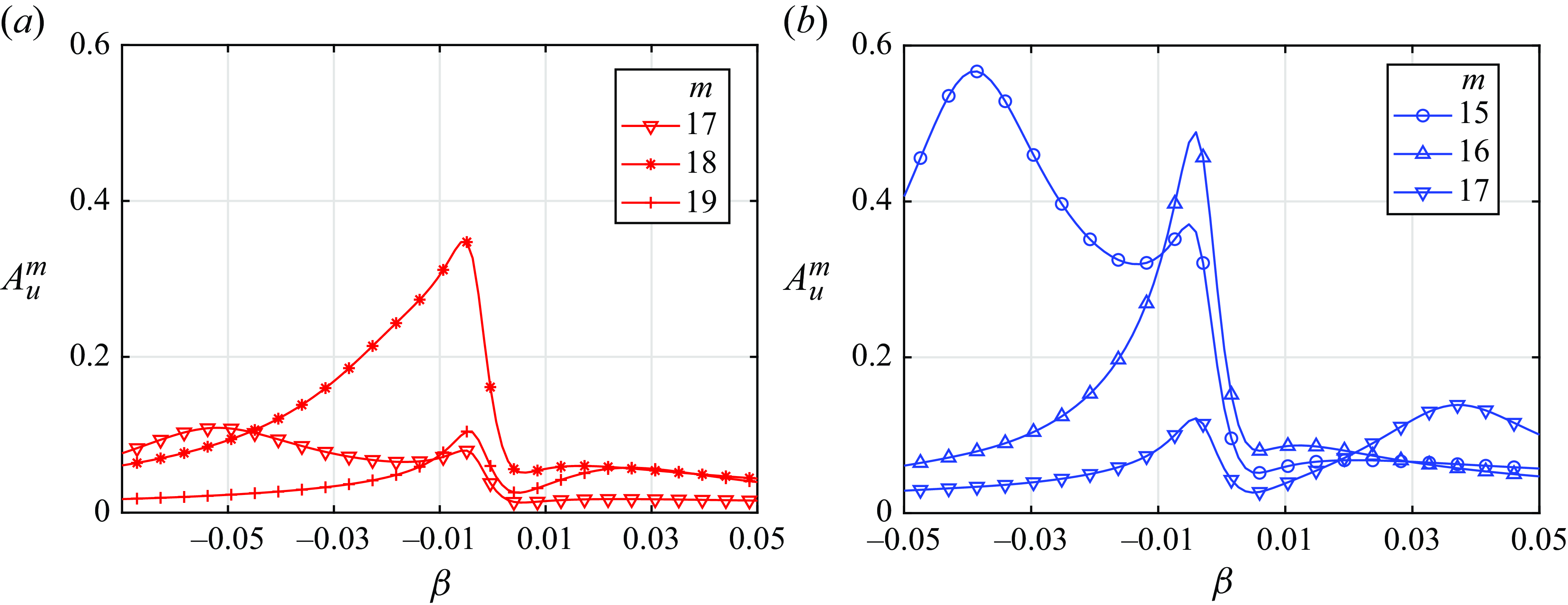
Figure 16. Amplitudes of horizontal velocity of dominant antisymmetric modes for (a) $\delta =0.2$
and (b)
$\delta =0.2$
and (b) $\delta =0.3$
.
$\delta =0.3$
.
Experimental validation of the predicted properties of the wavefield structure within a finite-thickness pycnocline cannot be obtained using the shadowgraph technique described in § 3. Therefore, additional series of measurements in which the PIV technique was applied have been performed.
5. Particle image velocimetry experiments
5.1. Procedure
The PIV set-up consists of a continuous 532 nm laser (1.5 W) with light sheet generation optics (see figure 1). To minimise the optical distortions caused by density gradient in the imaged area (Dalziel et al. Reference Dalziel, Hughes and Sutherland2000), the laser sheet is placed at a distance of 10 mm, sufficiently close to the front wall out of the Stokes layer. A 3.2 MPixel USB 3.1 camera (FLIR Blackfly) operating at 5 Hz recorded the flow field. Silver-coated hollow 10 μm glass spheres served as the tracers. LaVision Davis software was used to compute the two-dimensional instantaneous velocity field; the interrogation cell size was 48 $\times$
48 pixels with 50
$\times$
48 pixels with 50 $\%$
overlap, corresponding to a spatial resolution of 0.13 mm px−1. The temporal resolution defined by the camera frame rate corresponds to approximately 30 frames per wave period. The imaged area spans almost half a wavelength of the third standing-wave mode and is centred at its antinode. Supplementary movie 2 shows the maps of the vertical and horizontal velocity components normalised by the wavemaker velocity amplitude.
$\%$
overlap, corresponding to a spatial resolution of 0.13 mm px−1. The temporal resolution defined by the camera frame rate corresponds to approximately 30 frames per wave period. The imaged area spans almost half a wavelength of the third standing-wave mode and is centred at its antinode. Supplementary movie 2 shows the maps of the vertical and horizontal velocity components normalised by the wavemaker velocity amplitude.
The experiments were carried out for amplitude of the wavemaker displacement $F$
$F$ $ =7.5$
mm,
$ =7.5$
mm, $n$
$n$ $=3$
, forcing frequency corresponding to 0.905
$=3$
, forcing frequency corresponding to 0.905 $\leqslant \alpha \leqslant$
0.946 and
$\leqslant \alpha \leqslant$
0.946 and $0.18\lt$ $\delta$ $ {\lt } 0.43$
. As in the shadowgraph experiments, the mean position of the wavemaker centre was 350 mm above the bottom of the tank. Before each series of experiments, the basin was refilled as described in § 2. To decouple the effect of frequency detuning and the pycnocline thickness
$ {\lt } 0.43$
. As in the shadowgraph experiments, the mean position of the wavemaker centre was 350 mm above the bottom of the tank. Before each series of experiments, the basin was refilled as described in § 2. To decouple the effect of frequency detuning and the pycnocline thickness $d$
, in each series of PIV experiments, the forcing frequency was kept constant while in the course of the successive runs
$d$
, in each series of PIV experiments, the forcing frequency was kept constant while in the course of the successive runs $d$
gradually increased. At every
$d$
gradually increased. At every $\alpha$
, the experimental series consisted of 12–20 runs. The first run started from rest, then the wavemaker motion was initiated and lasted for 300 cycles; after that, the wavemaker stopped and paused for 10 min during which the waves fully decayed allowing the initiation of the next run. The density profile was measured by a PCP before the initiation of the series and between the runs at the end of the wavemaker pause.
$\alpha$
, the experimental series consisted of 12–20 runs. The first run started from rest, then the wavemaker motion was initiated and lasted for 300 cycles; after that, the wavemaker stopped and paused for 10 min during which the waves fully decayed allowing the initiation of the next run. The density profile was measured by a PCP before the initiation of the series and between the runs at the end of the wavemaker pause.
The consistency between PIV and shadowgraph measurements and the theoretical model is examined by the comparison of normalised vertical velocity amplitude distribution along the horizontal line ${\tilde {z}}=\delta$
in figure 17. The velocity amplitudes are normalised by the corresponding values at the third-mode antinode
${\tilde {z}}=\delta$
in figure 17. The velocity amplitudes are normalised by the corresponding values at the third-mode antinode $x/\lambda _3=0.5$
; the curves are plotted at the corresponding effective resonant conditions. A good agreement is observed, although the coverage of two experimental datasets is different.
$x/\lambda _3=0.5$
; the curves are plotted at the corresponding effective resonant conditions. A good agreement is observed, although the coverage of two experimental datasets is different.
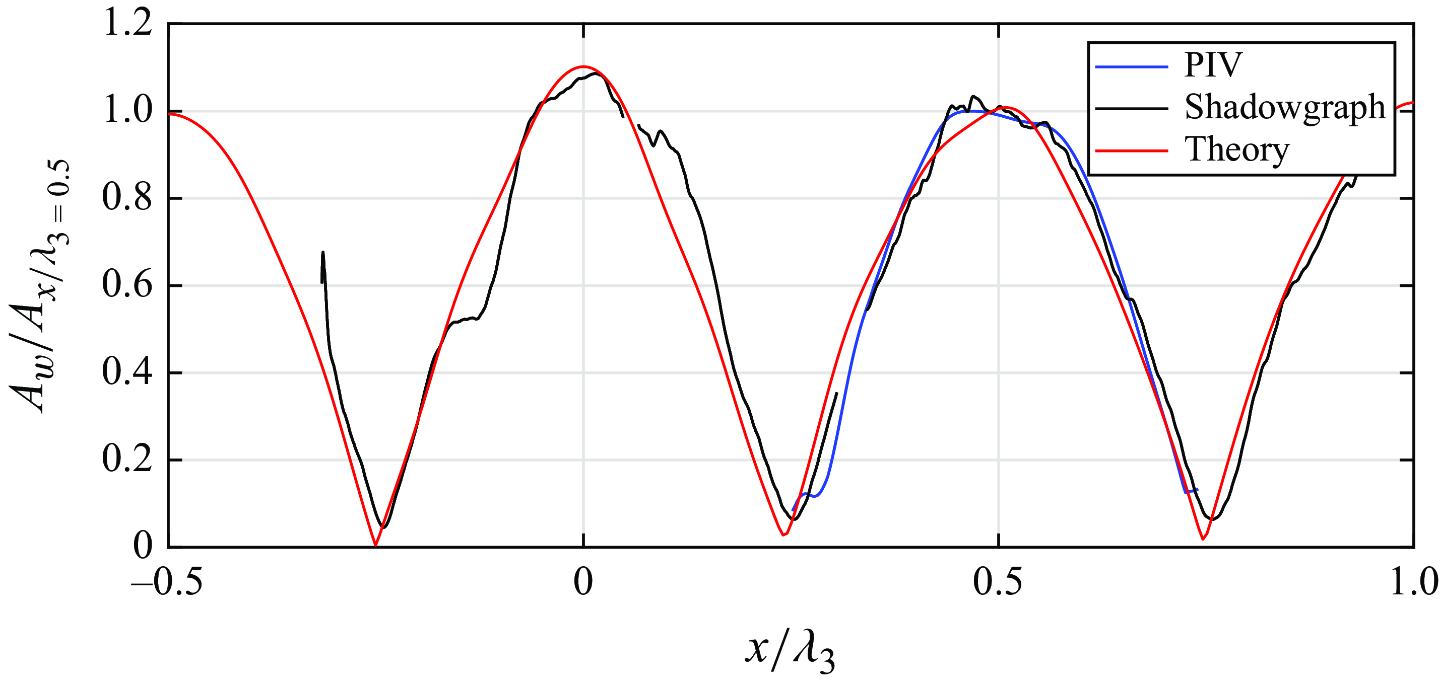
Figure 17. Vertical velocity amplitude along the upper pycnocline boundary ${\tilde {z}}=\delta$
, normalised by the corresponding value at
${\tilde {z}}=\delta$
, normalised by the corresponding value at $x/\lambda _3=0.5$
for PIVmeasurement, shadowgraph measurement and theory at the corresponding effective resonant conditions (
$x/\lambda _3=0.5$
for PIVmeasurement, shadowgraph measurement and theory at the corresponding effective resonant conditions ( $\alpha =0.917,$ $\delta$ $=0.32$
;
$=0.32$
; $\alpha =0.931,$ $\delta$ $=0.22$
;
$=0.22$
; $\alpha =0.925,$ $\delta$ $=0.306$
, respectively).
$=0.306$
, respectively).
Figure 18 presents a summary of the experimental conditions in the present experiments, along with the theoretically obtained dispersion relation $\alpha (k_3d)$
and the theoretical estimates of the effect of the finite wavemaker size and the dissipation. Each set of horizontal circles at a constant forcing frequency represents a single series of experimental runs as specified above. It demonstrates the natural widening of the pycnocline during each series. The colour of the circles corresponds to the amplitude of the vertical velocity oscillations at the antinode (
$\alpha (k_3d)$
and the theoretical estimates of the effect of the finite wavemaker size and the dissipation. Each set of horizontal circles at a constant forcing frequency represents a single series of experimental runs as specified above. It demonstrates the natural widening of the pycnocline during each series. The colour of the circles corresponds to the amplitude of the vertical velocity oscillations at the antinode ( $x/\lambda _3=0.5$
) after a quasi-steady state is attained for the given operational parameters.
$x/\lambda _3=0.5$
) after a quasi-steady state is attained for the given operational parameters.
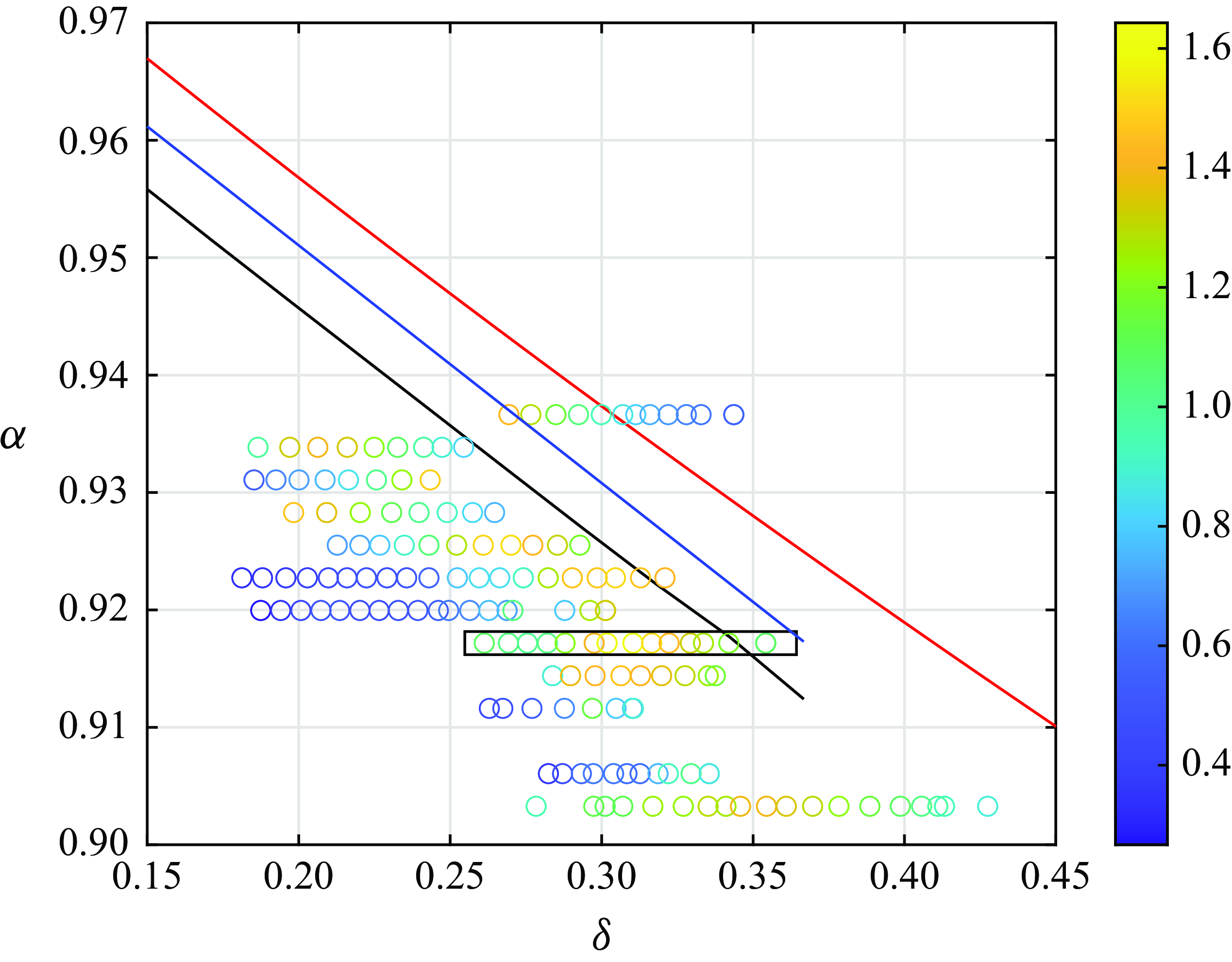
Figure 18. Diagram of the experimental conditions. The symbols represent the experimental results, with the colour showing the vertical velocity amplitude at the antinode ( $x/\lambda _3=0.5$
) normalised by the wavemaker velocity amplitude. The lines correspond to the eigenfrequency of the rectangular basin (red), the resonant frequency for the basin with the immersed wavemaker (blue) and the effective resonant frequency accounting for dissipation (black).
$x/\lambda _3=0.5$
) normalised by the wavemaker velocity amplitude. The lines correspond to the eigenfrequency of the rectangular basin (red), the resonant frequency for the basin with the immersed wavemaker (blue) and the effective resonant frequency accounting for dissipation (black).
5.2. Particle image velocimetry data analysis
5.2.1. Response curves
Numerous experiments carried out under diverse experimental conditions allow decoupling of the effect on the wavefield of the pycnocline thickness and of the forcing frequency. The horizontal and vertical sections of the diagram in figure 18 yield the experimentally measured variation of the system response to the forcing as a function of the dimensionless pycnocline thickness $\delta$
at fixed frequency, and of the dimensionless forcing frequency
$\delta$
at fixed frequency, and of the dimensionless forcing frequency $\alpha$
at fixed pycnocline thickness. Typical examples of the resulting curves are plotted in figure 19. The system response is represented by the amplitude of the vertical velocity component at the third-mode antinode normalised by the amplitude of the wavemaker velocity
$\alpha$
at fixed pycnocline thickness. Typical examples of the resulting curves are plotted in figure 19. The system response is represented by the amplitude of the vertical velocity component at the third-mode antinode normalised by the amplitude of the wavemaker velocity $A_w(x/\lambda _3=0.5,z=0)$
. The amplitude variation with the pycnocline thickness for a fixed frequency does not change notably with
$A_w(x/\lambda _3=0.5,z=0)$
. The amplitude variation with the pycnocline thickness for a fixed frequency does not change notably with $\alpha$
. The effective resonance frequency decreases with an increase in
$\alpha$
. The effective resonance frequency decreases with an increase in $\delta$
, while the maximum amplitude exhibits only a weak change. The normalised amplitude at the effective resonance is significantly smaller than those measured for the similarly excited surface waves (Mogilevskiy et al. Reference Mogilevskiy, Kalenko, Zemach and Shemer2024) that represent a limit case
$\delta$
, while the maximum amplitude exhibits only a weak change. The normalised amplitude at the effective resonance is significantly smaller than those measured for the similarly excited surface waves (Mogilevskiy et al. Reference Mogilevskiy, Kalenko, Zemach and Shemer2024) that represent a limit case $\delta$ $\to 0$
with negligible dissipation in the pycnocline.
$\to 0$
with negligible dissipation in the pycnocline.
The viscous model yields similar results (figure 20). The downshift of the effective resonance frequency is somewhat underestimated, while the normalised amplitude at the effective resonance is nearly twice larger than in the experiments. As in the experiments (figure 19
a), the maximum of the normalised amplitude practically does not vary with $\alpha$
.
$\alpha$
.
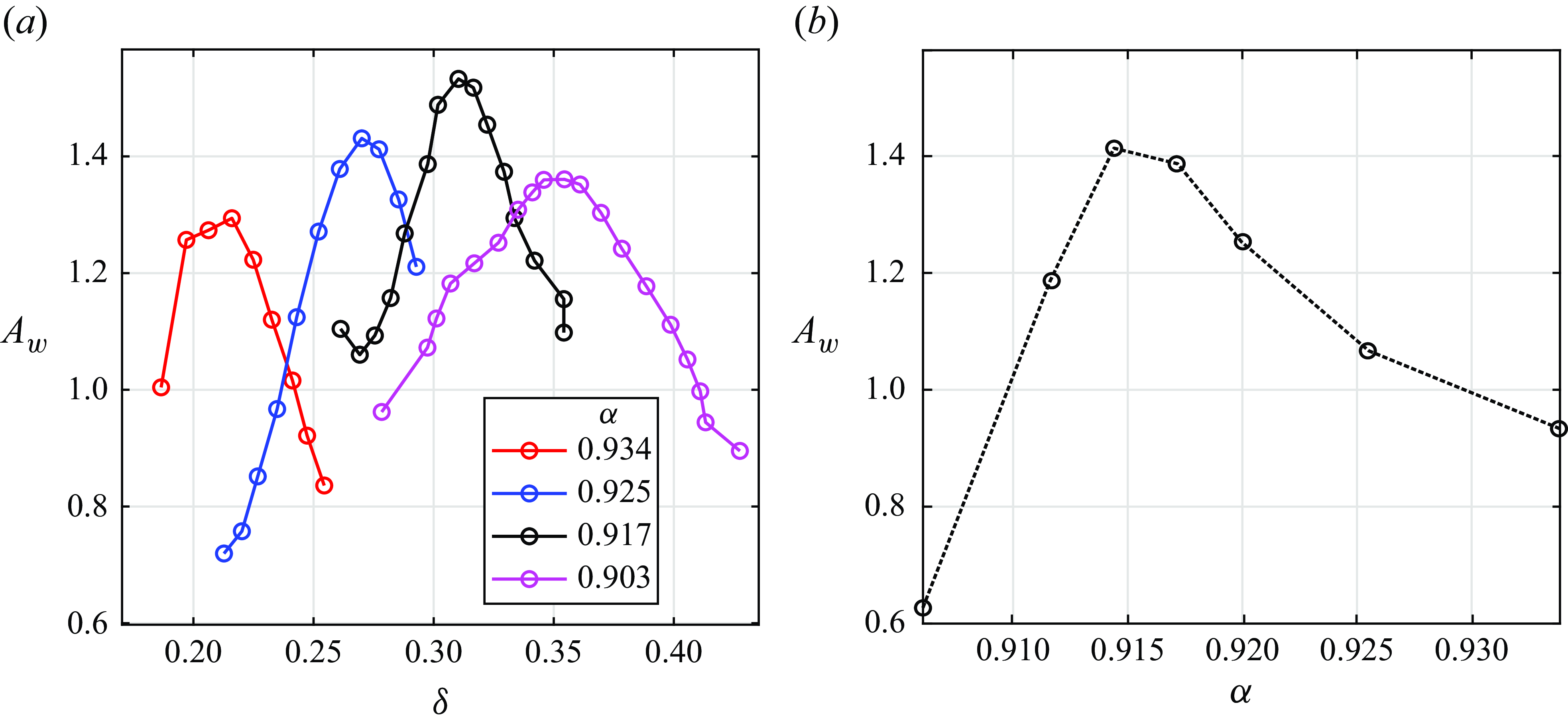
Figure 19. The amplitude of the vertical velocity oscillations at the antinode ( $x/\lambda _3=0.5$
) of the third-mode standing wave from PIV measurements: (a) as function of the pycnocline thickness for different forcing frequencies; (b) as function of frequency for constant pycnocline thickness
$x/\lambda _3=0.5$
) of the third-mode standing wave from PIV measurements: (a) as function of the pycnocline thickness for different forcing frequencies; (b) as function of frequency for constant pycnocline thickness $\delta$ $=0.305$
.
$=0.305$
.
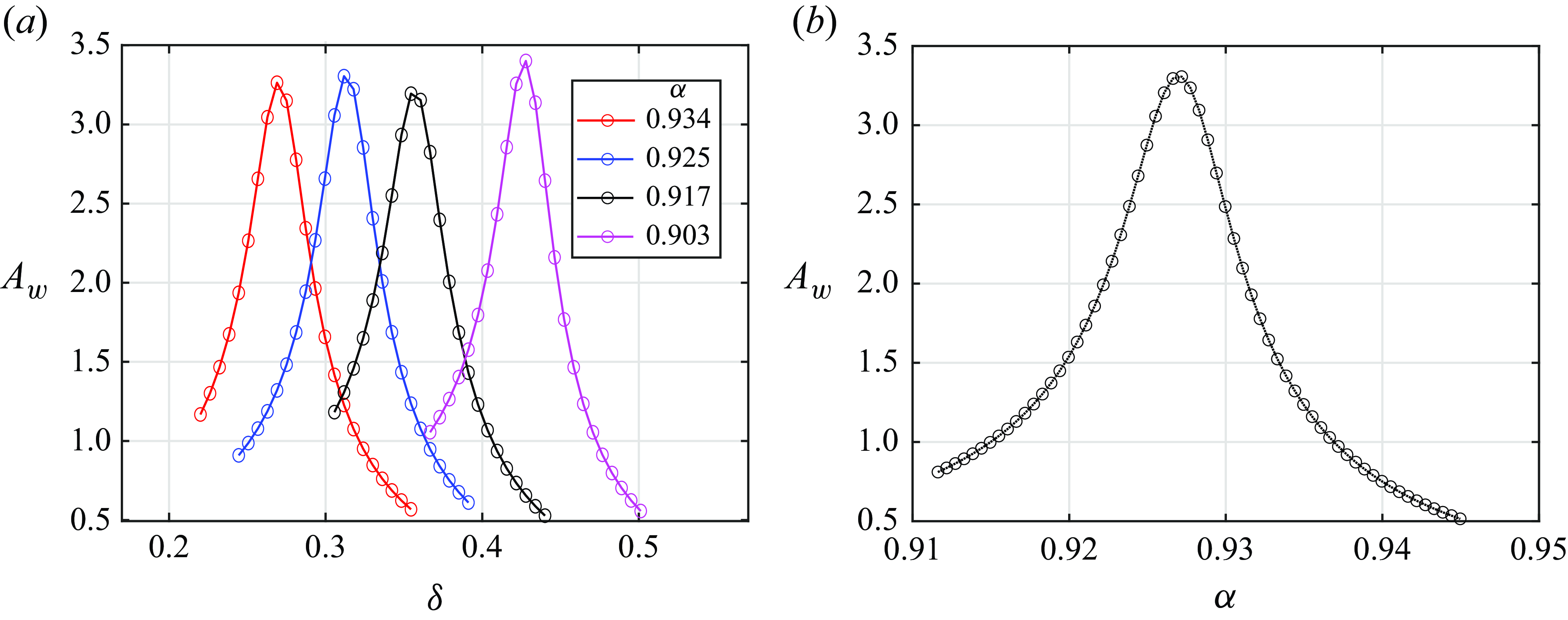
Figure 20. The results of the theoretical model accounting for the full dissipation for parameters as in figure 19.
Measurements of the vertical velocity amplitude at the antinode are summarised in figure 21 as a function of the detuning $\beta =\alpha -\alpha _*(\delta )$
. Note that the figure contains about 160 data points, each representing a separate experimental run more than 10 minutes long. Both shadowgraph- and PIV-derived results collapse onto close vicinity of a single curve. The measured data agree well with the linear theory (4.31) far below the resonance. The discrepancy of the measured maximum amplitude and of the corresponding detuning cannot be attributed solely to the effect of dissipation; thus, the effect of nonlinearity may also be significant. Indeed, selection of the value of the dissipation coefficient
$\beta =\alpha -\alpha _*(\delta )$
. Note that the figure contains about 160 data points, each representing a separate experimental run more than 10 minutes long. Both shadowgraph- and PIV-derived results collapse onto close vicinity of a single curve. The measured data agree well with the linear theory (4.31) far below the resonance. The discrepancy of the measured maximum amplitude and of the corresponding detuning cannot be attributed solely to the effect of dissipation; thus, the effect of nonlinearity may also be significant. Indeed, selection of the value of the dissipation coefficient $s$
to fit the maximum amplitude within the linear computational model does not cause a notable shift in the detuning at the effective resonance. To resolve this discrepancy by accounting for nonlinearity, advantage can be taken of close similarity between nonlinear resonant free-surface waves (Mogilevskiy et al. Reference Mogilevskiy, Kalenko, Zemach and Shemer2024) and those at the interface between the two liquids. Adjustments of their model to the present problem result in the estimation of the downshift of the effective resonance frequency
$s$
to fit the maximum amplitude within the linear computational model does not cause a notable shift in the detuning at the effective resonance. To resolve this discrepancy by accounting for nonlinearity, advantage can be taken of close similarity between nonlinear resonant free-surface waves (Mogilevskiy et al. Reference Mogilevskiy, Kalenko, Zemach and Shemer2024) and those at the interface between the two liquids. Adjustments of their model to the present problem result in the estimation of the downshift of the effective resonance frequency $(k_nF r^2/(h-\delta ))^{2/3}\approx 0.02,$
in good agreement with experiments.
$(k_nF r^2/(h-\delta ))^{2/3}\approx 0.02,$
in good agreement with experiments.
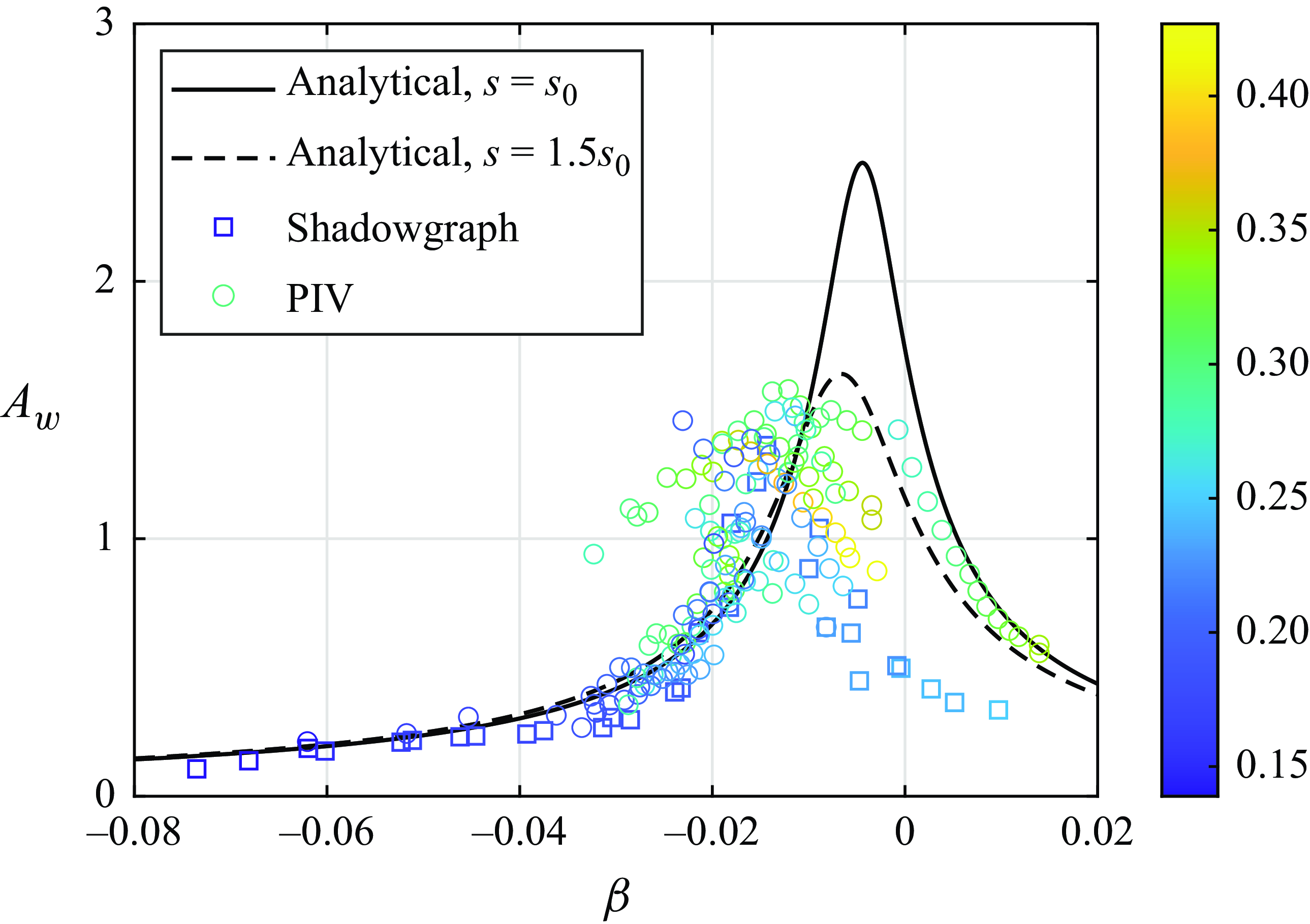
Figure 21. Normalised amplitude of the vertical velocity at the antinode as a function of the detuning. The colour of the experimental points corresponds to the pycnocline thickness $\delta$
; the value of dissipation coefficient
$\delta$
; the value of dissipation coefficient $s_0$
corresponds to experiments.
$s_0$
corresponds to experiments.
5.2.2. Symmetric and antisymmetric modes in the velocity field at the forcing frequency
The series of experimental runs carried out at a constant forcing frequency $\alpha =0.917$
(marked by a rectangular box in figure 18) is now considered. To analyse the wavefield at the forcing frequency, the PIV signal was band-pass-filtered at each spatial location
$\alpha =0.917$
(marked by a rectangular box in figure 18) is now considered. To analyse the wavefield at the forcing frequency, the PIV signal was band-pass-filtered at each spatial location $(x,z)$
independently, resulting in periodic in time functions:
$(x,z)$
independently, resulting in periodic in time functions:
 \begin{align} u^1(t,x,z)=A_u(x,z)\cos (\omega t+\theta _u),\quad w^1(t,x,z)=A_w(x,z)\cos (\omega t+\theta _w). \end{align}
The contour maps of the spatial distribution of the dimensionless amplitudes and phases of the vertical $w$
and the horizontal
$w$
and the horizontal $u$
velocity components are presented in figure 22. The distributions are dominated by the mode with
$u$
velocity components are presented in figure 22. The distributions are dominated by the mode with $m=3$
, although the short-scale features are also present.
$m=3$
, although the short-scale features are also present.
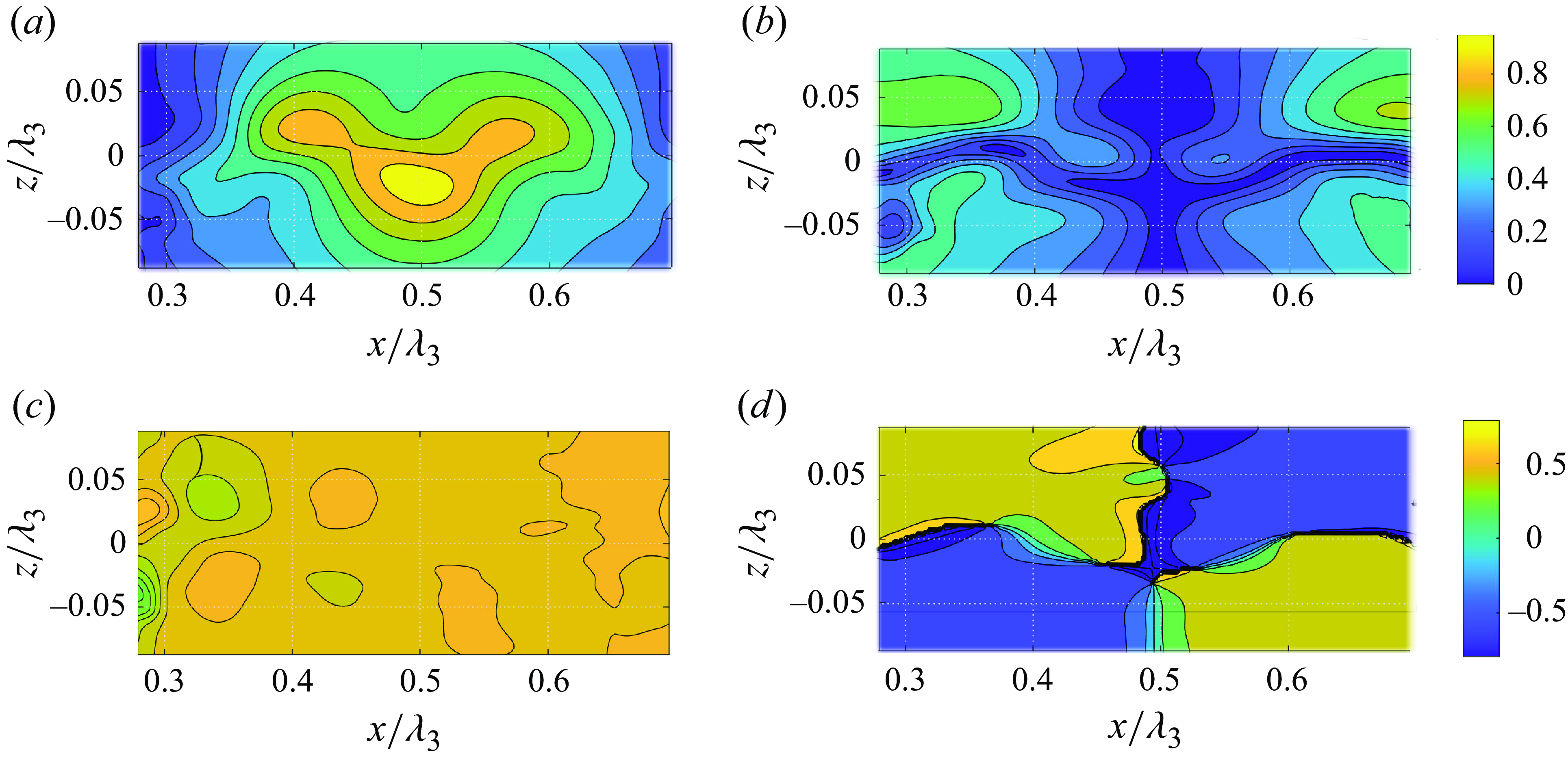
Figure 22. Spatial distributions of the velocity components for $\delta$ $=0.282$
band-pass-filtered at the forcing frequency
$=0.282$
band-pass-filtered at the forcing frequency $\alpha =0.917$
. (a,b) Amplitudes
$\alpha =0.917$
. (a,b) Amplitudes $A_{w,u}$
; (c,d) phase shift
$A_{w,u}$
; (c,d) phase shift $\theta _{w,u}$
in time (in
$\theta _{w,u}$
in time (in $\pi$
units) relative to the wavemaker displacement; (a,c) vertical velocity component
$\pi$
units) relative to the wavemaker displacement; (a,c) vertical velocity component $w$
; (b,d) horizontal velocity component
$w$
; (b,d) horizontal velocity component $u$
. Supplementary movie 3 shows the variation of maps of both band-pass-filtered velocity components.
$u$
. Supplementary movie 3 shows the variation of maps of both band-pass-filtered velocity components.
The dispersion relation (figure 12) indeed allows coexistence at the forcing frequency of the dominant symmetric mode with $m=3$
and of the higher antisymmetric modes with
$m=3$
and of the higher antisymmetric modes with $m$
ranging from 15to 17 (depending on the dimensionless pycnocline thickness
$m$
ranging from 15to 17 (depending on the dimensionless pycnocline thickness $\delta$
). To examine this conjecture, the third spatial mode is first identified in the recorded velocity distributions, and the assumption of the dominance of this standing-wave mode in the wavefield is verified. To this end, for each frame corresponding to instant
$\delta$
). To examine this conjecture, the third spatial mode is first identified in the recorded velocity distributions, and the assumption of the dominance of this standing-wave mode in the wavefield is verified. To this end, for each frame corresponding to instant $t$
and each
$t$
and each $z$
independently, the distributions of both velocity components normalised by the wavemaker velocity amplitude
$z$
independently, the distributions of both velocity components normalised by the wavemaker velocity amplitude $\omega F$
were fitted to
$\omega F$
were fitted to
 \begin{align} u^{fit}(t,x,z)=u_3(t,z)\cos (k_3 x+\gamma _u(t,z)),\!\!\!\quad w^{fit}(t,x,z)=w_3(t,z)\cos (k_3 x+\gamma _w(t,z)), \end{align}
defining functions $u^{fit}(t,x,z)$
and
$u^{fit}(t,x,z)$
and $w^{fit}(t,x,z)$
that are periodic in time with period
$w^{fit}(t,x,z)$
that are periodic in time with period $T_3$
and in the horizontal direction with the period
$T_3$
and in the horizontal direction with the period $\lambda _3$
;
$\lambda _3$
; $u_3(t,z)$
,
$u_3(t,z)$
, $w_3(t,z)$
,
$w_3(t,z)$
, $\gamma _u(t,z)$
and
$\gamma _u(t,z)$
and $\gamma _w(t,z)$
are the fitting parameters. For each location
$\gamma _w(t,z)$
are the fitting parameters. For each location $(x,z)$
, the time-dependent periodic functions
$(x,z)$
, the time-dependent periodic functions $u^{fit}$
and
$u^{fit}$
and $w^{fit}$
have amplitudes
$w^{fit}$
have amplitudes $A_{u,w}^{fit}(x,z)$
and phase shift
$A_{u,w}^{fit}(x,z)$
and phase shift $\theta _{u,w}^{fit}(x,z)$
relative to the wavemaker displacement plotted in figure 23. The patterns of the phase maps correspond to the third-mode standing wave with a practically constant
$\theta _{u,w}^{fit}(x,z)$
relative to the wavemaker displacement plotted in figure 23. The patterns of the phase maps correspond to the third-mode standing wave with a practically constant $\theta _{w}^{fit}(x,z)$
. The values of
$\theta _{w}^{fit}(x,z)$
. The values of $\theta _{u}^{fit}(x,z)$
change sharply by
$\theta _{u}^{fit}(x,z)$
change sharply by $\pi$
in the vicinity of the corresponding nodes.
$\pi$
in the vicinity of the corresponding nodes.


The profiles of the normalised vertical velocity component amplitude $A_w(x,z)$
at the antinode
$A_w(x,z)$
at the antinode $x/\lambda _3=0.5$
of the band-pass-filtered record (figure 24
a) are compared with the corresponding distributions of the normalised fitted amplitudes
$x/\lambda _3=0.5$
of the band-pass-filtered record (figure 24
a) are compared with the corresponding distributions of the normalised fitted amplitudes $A_w^{fit}$
(figure 24
b) at multiple experimental runs with different values of the pycnocline thickness
$A_w^{fit}$
(figure 24
b) at multiple experimental runs with different values of the pycnocline thickness $\delta$
. The shapes of the velocity amplitude profiles
$\delta$
. The shapes of the velocity amplitude profiles $A_{w}(z)$
differ notably from those of the fitted distributions. The profiles obtained for different experimental conditions
$A_{w}(z)$
differ notably from those of the fitted distributions. The profiles obtained for different experimental conditions $A_w^{fit}$
appear to be symmetric around
$A_w^{fit}$
appear to be symmetric around $z=0$
; when normalised by their maxima, they nearly collapse, with shapes that agree well with the theoretical eigenfunction of the third mode (figure 24
c).
$z=0$
; when normalised by their maxima, they nearly collapse, with shapes that agree well with the theoretical eigenfunction of the third mode (figure 24
c).
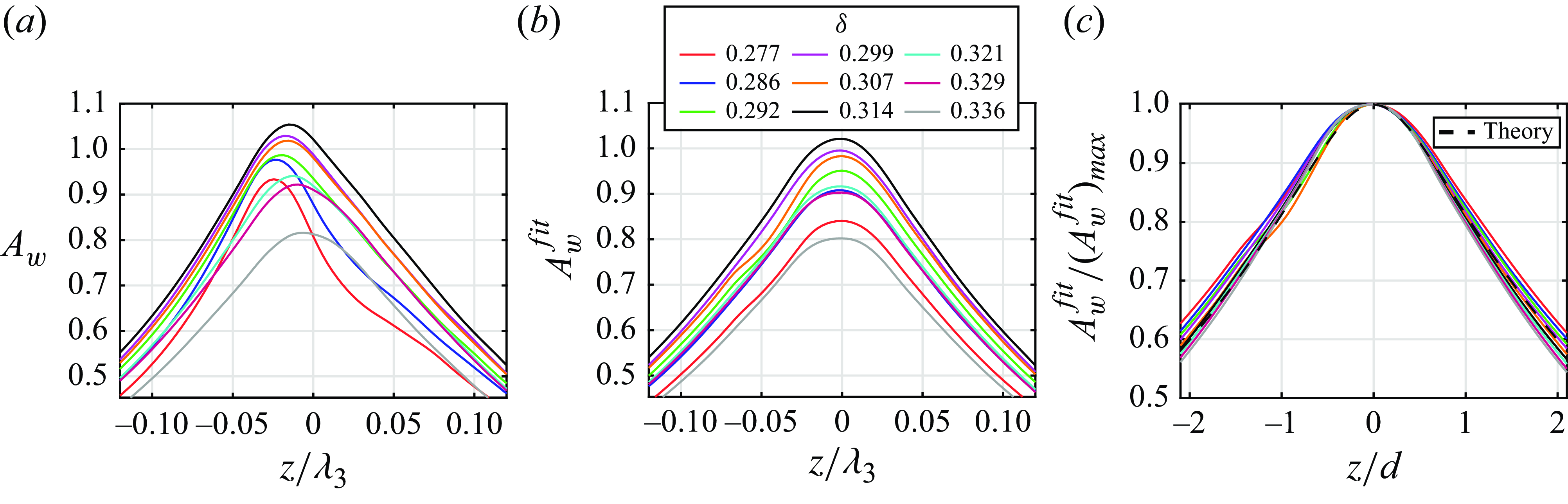
Figure 24. (a) Profiles of the vertical velocity component amplitude. (b) The fitted amplitude of the third-mode wave for different pycnocline thickness $\delta$
. (c) The fitted distributions normalised by their maxima are compared with theoretical eigenfunction for
$\delta$
. (c) The fitted distributions normalised by their maxima are compared with theoretical eigenfunction for $m=3$
,
$m=3$
, $\delta$ $=0.305$
and
$=0.305$
and $\alpha =0.917$
(the black bold dashed line).
$\alpha =0.917$
(the black bold dashed line).
The contribution to the wavefield of the antisymmetric modes at the wavemaker forcing frequency is evaluated by computing at each instant the residual defined as
 \begin{align} u^{res}(t,x,z)=u^1-u^{fit},\quad w^{res}(t,x,z)=w^1-w^{fit}. \end{align}
The maps of amplitudes $A_{w,u}^{res}$
of the vertical and horizontal velocity components
$A_{w,u}^{res}$
of the vertical and horizontal velocity components $w^{res}$
and
$w^{res}$
and $u^{res}$
presented in figure 25(a,b) exhibit a spatially quasi-periodic horizontal structure, with mean wavelength corresponding to
$u^{res}$
presented in figure 25(a,b) exhibit a spatially quasi-periodic horizontal structure, with mean wavelength corresponding to $m$
about 16, in agreement with the dispersion relation (figure 12). Note that the amplitudes
$m$
about 16, in agreement with the dispersion relation (figure 12). Note that the amplitudes $A_w^{res}$
of the residual of the vertical velocity component
$A_w^{res}$
of the residual of the vertical velocity component $w^{res}$
practically vanish along the centreline of the pycnocline
$w^{res}$
practically vanish along the centreline of the pycnocline $z=0$
, where the maxima of the horizontal velocity amplitudes
$z=0$
, where the maxima of the horizontal velocity amplitudes $A_u^{res}$
are located. The corresponding phase maps are presented in figure 25(c) and 25(d), respectively. The phase shift of
$A_u^{res}$
are located. The corresponding phase maps are presented in figure 25(c) and 25(d), respectively. The phase shift of $\pi$
between the two maxima of the residual of the vertical velocity amplitude confirms that the wave is antisymmetric around
$\pi$
between the two maxima of the residual of the vertical velocity amplitude confirms that the wave is antisymmetric around $z=0$
.
$z=0$
.


The estimated vertical profiles of the normalised amplitudes of the residuals of the vertical and horizontal velocity components are now compared with the theoretical eigenmodes for $m=16$
for different values of the pycnocline thickness
$m=16$
for different values of the pycnocline thickness $\delta$
. The profiles are plotted for the antinode locations of the corresponding velocity components:
$\delta$
. The profiles are plotted for the antinode locations of the corresponding velocity components: $x/\lambda _3=0.5$
and
$x/\lambda _3=0.5$
and $x/\lambda _3=0.537$
, respectively (figure 26
a,b). The theoretical curve computed for
$x/\lambda _3=0.537$
, respectively (figure 26
a,b). The theoretical curve computed for $m=16$
and
$m=16$
and $k_3d=0.306$
is compared with the experimental profiles normalised by their maxima and agree reasonably well.
$k_3d=0.306$
is compared with the experimental profiles normalised by their maxima and agree reasonably well.
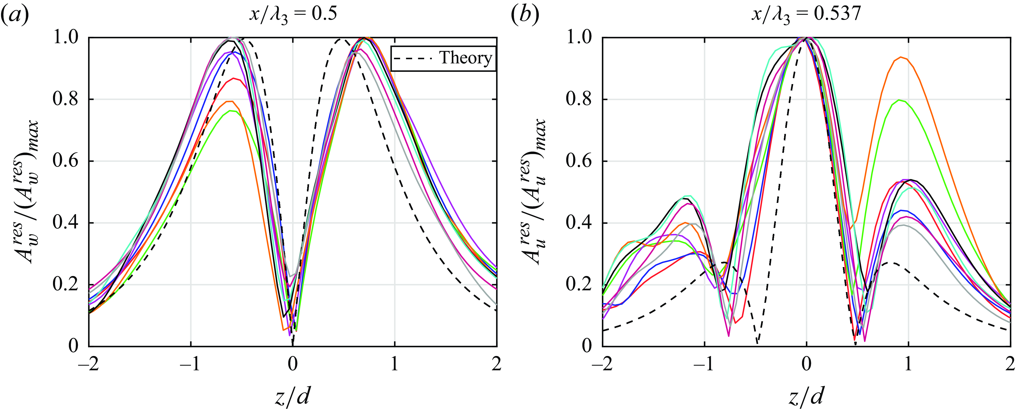
Figure 26. Profiles of normalised amplitudes of (a) residual vertical velocity component at $x/\lambda _3=0.5$
and (b) residual horizontal velocity component at
$x/\lambda _3=0.5$
and (b) residual horizontal velocity component at $x/\lambda _3=0.537$
for different pycnocline thickness. In (a,b), theoretical curves correspond to
$x/\lambda _3=0.537$
for different pycnocline thickness. In (a,b), theoretical curves correspond to $m=16$
and
$m=16$
and $\delta$ $=0.306$
; colours as in figure 24.
$=0.306$
; colours as in figure 24.
The adopted data processing procedure allows decomposition of the complex wavefield into coexisting different symmetric and antisymmetric spatial modes at the single forcing frequency. The wave is dominated by a single symmetric eigenmode, over which a weaker and shorter antisymmetric wave is superposed. The effective wavemode number $m$
of the antisymmetric mode was obtained from the mean distance between the consecutive maxima of the residual vertical velocity amplitude (figure 25
a). The measured values agree with the theoretically predicted values based on the dispersion relation for the range of
$m$
of the antisymmetric mode was obtained from the mean distance between the consecutive maxima of the residual vertical velocity amplitude (figure 25
a). The measured values agree with the theoretically predicted values based on the dispersion relation for the range of $\alpha$
and
$\alpha$
and $\delta$
adopted in the experiments (figures 12
a and 27
a). The variation of the measured normalised amplitudes of the antisymmetric mode with the pycnocline thickness
$\delta$
adopted in the experiments (figures 12
a and 27
a). The variation of the measured normalised amplitudes of the antisymmetric mode with the pycnocline thickness $\delta$
for different constant forcing frequencies is presented in figure 27(b).
$\delta$
for different constant forcing frequencies is presented in figure 27(b).

Figure 27. (a) Normalised frequency $\alpha$
as a function of
$\alpha$
as a function of $\delta$
for antisymmetric modes with
$\delta$
for antisymmetric modes with $15\leqslant m \leqslant 17$
. The markers correspond to the experimentally observed modes. (b) The response curves of the antisymmetric mode as a function of the pycnocline thickness
$15\leqslant m \leqslant 17$
. The markers correspond to the experimentally observed modes. (b) The response curves of the antisymmetric mode as a function of the pycnocline thickness $\delta$
for different values of
$\delta$
for different values of $\alpha$
.
$\alpha$
.
5.2.3. Second frequency harmonic
The shadowgraph experiments presented in § 3 indicate that the interface has a complex structure not just in space but also in time, with the second harmonic in the frequency that cannot be neglected (figure 8). Its excitation can be attributed to nonlinear interaction of the primary wave with itself, as well as to the temporal variation of the wavemaker immersion depth relative to the pycnocline; see (4.5b ) and boundary condition (4.6d ) that account for the variable wavemaker position.
The PIV-derived temporal variation of the vertical velocity component measured at the third-mode antinode $x/\lambda _3=0.5$
is dominated by the contributions of the two lowest-frequency harmonics
$x/\lambda _3=0.5$
is dominated by the contributions of the two lowest-frequency harmonics $\alpha$
and
$\alpha$
and $2\alpha$
. Figure 28 supports this statement for the forcing frequency
$2\alpha$
. Figure 28 supports this statement for the forcing frequency $\alpha =0.917$
and different values of
$\alpha =0.917$
and different values of $\delta$
.
$\delta$
.
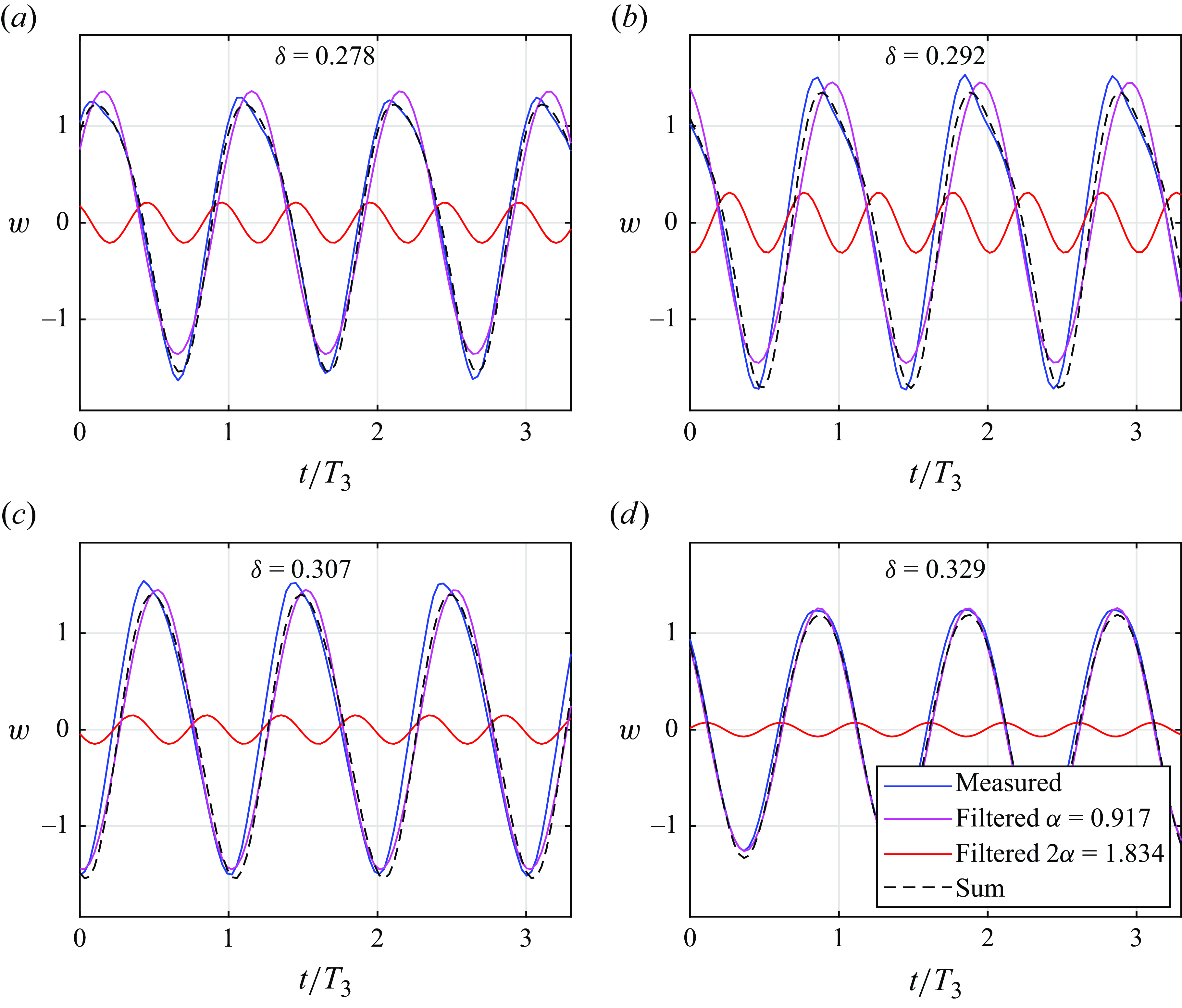
Figure 28. Decomposition of the temporal record of vertical velocity into that at forcing frequency $\alpha$
and at double that frequency
$\alpha$
and at double that frequency $2\alpha$
for (a–d) different values of
$2\alpha$
for (a–d) different values of $\delta$
.
$\delta$
.
The main features of the second harmonic can be predicted based on the linear dispersion relation (figure 12
a). A contour map of the vertical velocity component amplitude band-pass-filtered at double the wavemaker frequency presented in figure 29(a) is characterised by a quasi-periodic wave pattern. The vertical amplitude profile has a single maximum within the pycnocline at $z\approx 0$
which is a fingerprint of a symmetric eigenmode. The estimated mode number
$z\approx 0$
which is a fingerprint of a symmetric eigenmode. The estimated mode number $m\approx 20$
is in agreement the linear theory. The two-layer model predicts a second-harmonic wave with mode number
$m\approx 20$
is in agreement the linear theory. The two-layer model predicts a second-harmonic wave with mode number $m=12$
; accounting for the finite thickness of the pycnocline upshifts the resonant mode number considerably. For the range of
$m=12$
; accounting for the finite thickness of the pycnocline upshifts the resonant mode number considerably. For the range of $\delta$
and
$\delta$
and $\alpha$
in the present experiments, the slope of the dispersion curve in figure 12(a) at the vicinity of
$\alpha$
in the present experiments, the slope of the dispersion curve in figure 12(a) at the vicinity of $m$
corresponding to the second frequency harmonic is quite small. This enables coexistence in the wavefield of multiple neighbouring resonant standing modes, resulting in complex measured spatial distributions of the vertical velocity component amplitudes (figure 29
b).
$m$
corresponding to the second frequency harmonic is quite small. This enables coexistence in the wavefield of multiple neighbouring resonant standing modes, resulting in complex measured spatial distributions of the vertical velocity component amplitudes (figure 29
b).

Figure 29. (a) Contour map of vertical velocity amplitude of the second harmonic $A_w^{(2)}$
(normalised by the wavemaker velocity amplitude) for
$A_w^{(2)}$
(normalised by the wavemaker velocity amplitude) for $\delta$ $=0.342$
and
$=0.342$
and $\alpha =0.903$
. (b) The spatial distribution of the normalised amplitude profiles of the second harmonic of the vertical velocity component at
$\alpha =0.903$
. (b) The spatial distribution of the normalised amplitude profiles of the second harmonic of the vertical velocity component at $z=0$
, for different
$z=0$
, for different $\delta$
. Supplementary movie 6 shows the temporal variation of the map of the band-pass-filtered vertical component.
$\delta$
. Supplementary movie 6 shows the temporal variation of the map of the band-pass-filtered vertical component.
6. Conclusions
This study is focused on two-dimensional internal resonant standing waves excited by a cylinder vertically oscillating in a narrow deep basin with length $L$
in the vicinity of the basin’s eigenfrequencies. The basin is filled by stable layers of salted and pure water separated by a thin pycnocline of finite thickness
$L$
in the vicinity of the basin’s eigenfrequencies. The basin is filled by stable layers of salted and pure water separated by a thin pycnocline of finite thickness $d$
. The waves in such a system differ qualitatively from those observed at the interface of two immiscible fluids (Mogilevskiy et al. Reference Mogilevskiy, Kalenko, Zemach and Shemer2024), as well as from internal waves within a fluid with a constant density gradient (Thorpe Reference Thorpe1968). For the pycnocline-type density distribution employed in the present study, multiple wavenumbers satisfy the dispersion relation for any given frequency (see § 4.2). Thus, a temporally monochromatic forcing excites a wavefield with a complex spatial structure that, in the steady regime, comprises multiple possible standing waves at the forcing frequency. Fourier analyses in frequency or wavenumber domains are applied to reveal the spatial and temporal structures of the waves. Wave amplitudes in frequency and in wavenumber domains, the effective resonance frequencies and the maximum possible system responses for a given wavemaker displacement amplitude are defined by dimensionless pycnocline thickness
$d$
. The waves in such a system differ qualitatively from those observed at the interface of two immiscible fluids (Mogilevskiy et al. Reference Mogilevskiy, Kalenko, Zemach and Shemer2024), as well as from internal waves within a fluid with a constant density gradient (Thorpe Reference Thorpe1968). For the pycnocline-type density distribution employed in the present study, multiple wavenumbers satisfy the dispersion relation for any given frequency (see § 4.2). Thus, a temporally monochromatic forcing excites a wavefield with a complex spatial structure that, in the steady regime, comprises multiple possible standing waves at the forcing frequency. Fourier analyses in frequency or wavenumber domains are applied to reveal the spatial and temporal structures of the waves. Wave amplitudes in frequency and in wavenumber domains, the effective resonance frequencies and the maximum possible system responses for a given wavemaker displacement amplitude are defined by dimensionless pycnocline thickness $\delta$
and affected by dissipation. An increase in
$\delta$
and affected by dissipation. An increase in $\delta$
downshifts the effective resonance frequency from that given by the two-layer model (equation (2.1)). Additional non-negligible spatial modes at the second temporal harmonic are excited as well.
$\delta$
downshifts the effective resonance frequency from that given by the two-layer model (equation (2.1)). Additional non-negligible spatial modes at the second temporal harmonic are excited as well.
The developed linear model yields estimates of the effect of the pycnocline thickness and of the finite size of the vertically oscillating cylindrical wavemaker on the structure of the internal wavefield resonantly excited in a narrow rectangular basin. The model accounts for the dissipation in the Stokes layers at the solid surfaces and in the bulk within the pycnocline (§ 4.4). The resulting wavefield involves superposition of two types of internal waves that correspond to symmetric and antisymmetric distributions of the vertical velocity, as followed by the analysis based on the Taylor–Goldstein equation (4.14). The model predicts how the amplitudes of both symmetric and antisymmetric modes depend on the forcing frequency. The symmetric mode amplitudes effectively depend only on the dimensionless detuning $\beta$
(4.29), that is, the normalised deviation of the forcing frequency from the pycnocline thickness-dependent eigenfrequency (figure 15). Similarly to the case of resonant free-surface gravity waves, the finite size of the wavemaker leads to a certain downshift of eigenfrequencies. Antisymmetric modes are characterised by a different behaviour (figure 16); the wavenumber of the antisymmetric mode with the highest amplitudes changes with the detuning. The theoretical findings are compared with the results of experiments. Each experimental session consisted of a sequence of runs spanning frequencies in the vicinity of the effective resonance. Between the consecutive runs, the wavemaker was stopped for a duration sufficient for the liquid to come to rest. The measurements of the detailed vertical density profile carried out during these pauses detected broadening of the pycnocline in the course of each session.
$\beta$
(4.29), that is, the normalised deviation of the forcing frequency from the pycnocline thickness-dependent eigenfrequency (figure 15). Similarly to the case of resonant free-surface gravity waves, the finite size of the wavemaker leads to a certain downshift of eigenfrequencies. Antisymmetric modes are characterised by a different behaviour (figure 16); the wavenumber of the antisymmetric mode with the highest amplitudes changes with the detuning. The theoretical findings are compared with the results of experiments. Each experimental session consisted of a sequence of runs spanning frequencies in the vicinity of the effective resonance. Between the consecutive runs, the wavemaker was stopped for a duration sufficient for the liquid to come to rest. The measurements of the detailed vertical density profile carried out during these pauses detected broadening of the pycnocline in the course of each session.
Two independent series of experiments were carried out. First, video shadowgraphy was used in which dye was added to the salted water resulting in a clearly visible sharp interface that was captured by a video camera over nearly the whole span of the basin. The density profile measurements relate this interface to the upper boundary of the pycnocline. The temporal and the spatial variation of the recorded shape of the interface is dominated by the resonant third mode; the interface, however, also exhibits features with shorter length scales. The frequency spectra of the interface movement at any fixed lateral location $x$
contain a major contribution at the forcing frequency, with a notable peak at its second harmonic. When all frequencies but the forcing frequency are removed by applying band-pass filtering at each lateral location separately, the wavenumber spectra of the resulting interfaces exhibit three peaks. The main peak is centred at the resonant mode; two other relatively broad peaks may be attributed to the cubic nonlinearity (mode numbers around 9) and to the presence of the antisymmetric modes with numbers around 15.
$x$
contain a major contribution at the forcing frequency, with a notable peak at its second harmonic. When all frequencies but the forcing frequency are removed by applying band-pass filtering at each lateral location separately, the wavenumber spectra of the resulting interfaces exhibit three peaks. The main peak is centred at the resonant mode; two other relatively broad peaks may be attributed to the cubic nonlinearity (mode numbers around 9) and to the presence of the antisymmetric modes with numbers around 15.
To study the internal structure of the waves within the pycnocline that cannot be revealed by shadowgraphy, the instantaneous spatial distributions of both velocity components were measured using the time-resolved PIV technique in a separate series of experiments. To resolve the wavefield within the relatively thin pycnocline, the spatial coverage of the PIV images was reduced as compared with that in shadowgraph experiments; it was centred horizontally at the antinode of the dominant wave. In each experimental session, the forcing frequency was retained constant. Consecutive runs thus allowed the study of the variation of the system response with growing-in-time thickness of the pycnocline $d$
. Multiple series carried out at different frequencies allowed extraction of the response curves as a function of frequency for different values of
$d$
. Multiple series carried out at different frequencies allowed extraction of the response curves as a function of frequency for different values of $d$
. The measured values of the effective resonant frequencies and of the maximum wave amplitudes are somewhat lower than the predictions of the linear model even though it accounts for dissipation. The estimates based on the analogy between the internal and the free-surface two-dimensional resonant standing waves allowed attribution of the observed downshift to nonlinear effects.
$d$
. The measured values of the effective resonant frequencies and of the maximum wave amplitudes are somewhat lower than the predictions of the linear model even though it accounts for dissipation. The estimates based on the analogy between the internal and the free-surface two-dimensional resonant standing waves allowed attribution of the observed downshift to nonlinear effects.
A special data processing procedure has been developed to analyse the considerable body of data accumulated in the present experiments. The PIV-measured data were used to reveal the temporal and the spatial wave structure within the pycnocline. At the forcing frequency, the contributions of the long symmetric and the short antisymmetric modes are identified. The maps of the obtained amplitude distributions (figure 22) agree well with the theoretical prediction based on the Taylor–Goldstein equation. The difference between the full band-pass-filtered maps and those corresponding to the third mode only (figure 25) shows remarkable similarity to the antisymmetric eigenmodes at the corresponding eigenfrequency, with mode number $m$
ranging from 15to 17, depending on
$m$
ranging from 15to 17, depending on $d$
. The maps of the amplitudes of the velocity component distributions obtained by band-pass filtering around double the forcing frequency (figure 29) are dominated by the symmetric mode with mode number
$d$
. The maps of the amplitudes of the velocity component distributions obtained by band-pass filtering around double the forcing frequency (figure 29) are dominated by the symmetric mode with mode number $m\approx 20$
, in agreement with the Taylor–Goldstein equation.
$m\approx 20$
, in agreement with the Taylor–Goldstein equation.
Supplementary material
Supplementary material are available at https://doi.org/10.1017/jfm.2025.384
Acknowledgements
E.M. thanks the Center for Integration in Science of the Israeli Ministry of Aliyah and Integration for support.
Funding
This research was supported by Pazy Foundation (grant no. 5100034339) and by Israel Science Foundation (grant no. 735/23).
Declaration of interests
The authors report no conflict of interest.
Appendix A. Viscous dissipation
The non-slip conditions at the front and back walls $y=0$
and
$y=0$
and $y=B=160$
mm render the flow of viscous liquid in the system three-dimensional. Nevertheless, since the pressure remains constant across the Stokes boundary layers at the walls, the solution with two non-zero velocity components is feasible. The governing equations get additional terms due to the viscous stresses proportional to the dynamic viscosity
$y=B=160$
mm render the flow of viscous liquid in the system three-dimensional. Nevertheless, since the pressure remains constant across the Stokes boundary layers at the walls, the solution with two non-zero velocity components is feasible. The governing equations get additional terms due to the viscous stresses proportional to the dynamic viscosity $\mu$
:
$\mu$
:
 \begin{equation} \begin{array}{c} \displaystyle {\rho _0\frac {\partial u}{\partial t}=-\frac {\partial p}{\partial x}+\mu \left [\frac {\partial ^2 u}{\partial x^2}+\frac {\partial ^2 u}{\partial y^2}+\frac {\partial ^2 u}{\partial z^2}\right ]},\\ \\ \displaystyle {\rho _0\frac {\partial w}{\partial t}=-\frac {\partial p}{\partial z}-\rho g+\mu \left [\frac {\partial ^2 w}{\partial x^2}+\frac {\partial ^2 w}{\partial y^2}+\frac {\partial ^2 w_d}{\partial z^2}\right ]},\\ \\ \displaystyle {\frac {\partial \rho }{\partial \tau }+w\frac {d\rho _s(z)}{dz}=0},\\ \\ \displaystyle {\frac {\partial u}{\partial x}+\frac {\partial w}{\partial z}=0,}\\ \end{array} \end{equation}
where $\rho _s(z)$
is the mean density distribution and
$\rho _s(z)$
is the mean density distribution and $\rho _0=(\rho _1+\rho _2)/2$
. The viscosity
$\rho _0=(\rho _1+\rho _2)/2$
. The viscosity $\mu$
is assumed constant. Averaging the equations over
$\mu$
is assumed constant. Averaging the equations over $y\in (0,B)$
results in
$y\in (0,B)$
results in
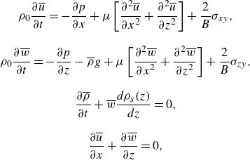 \begin{equation} \begin{array}{c} \displaystyle {\rho _0\frac {\partial \overline {u}}{\partial t}=-\frac {\partial p}{\partial x}+\mu \left [\frac {\partial ^2 \overline {u}}{\partial x^2}+\frac {\partial ^2 \overline {u}}{\partial z^2}\right ]+\frac {2}{B}\sigma _{xy}},\\ \\ \displaystyle {\rho _0\frac {\partial \overline {w}}{\partial t}=-\frac {\partial p}{\partial z}-\overline {\rho }g+\mu \left [\frac {\partial ^2 \overline {w}}{\partial x^2}+\frac {\partial ^2 \overline {w}}{\partial z^2}\right ]+\frac {2}{B}\sigma _{zy}},\\ \\ \displaystyle {\frac {\partial \overline {\rho }}{\partial t}+\overline {w}\frac {d\rho _s(z)}{dz}=0},\\ \\ \displaystyle {\frac {\partial \overline {u}}{\partial x}+\frac {\partial \overline {w}}{\partial z}=0,}\\ \end{array} \end{equation}
where $\sigma _{xy}=\mu \partial \overline {u}/\partial y$
and
$\sigma _{xy}=\mu \partial \overline {u}/\partial y$
and $\sigma _{zy}=\mu \partial \overline {w}/\partial y$
are viscous stresses at each wall. It is assumed that the Stokes layer thickness
$\sigma _{zy}=\mu \partial \overline {w}/\partial y$
are viscous stresses at each wall. It is assumed that the Stokes layer thickness $\sqrt {\mu /\rho _0\omega }\sim 1$
mm is much smaller than the basin width
$\sqrt {\mu /\rho _0\omega }\sim 1$
mm is much smaller than the basin width $B$
, and the averaged values differ insignificantly from those in the middle of the basin; the overbars are omitted in the following. The viscous stresses are calculated for time-periodic flow from the consideration of the Stokes layer in time-periodic flow (Mei Reference Mei1989). The complex amplitudes of the stresses
$B$
, and the averaged values differ insignificantly from those in the middle of the basin; the overbars are omitted in the following. The viscous stresses are calculated for time-periodic flow from the consideration of the Stokes layer in time-periodic flow (Mei Reference Mei1989). The complex amplitudes of the stresses $\hat {\sigma }_{xy}$
and
$\hat {\sigma }_{xy}$
and $\hat {\sigma }_{zy}$
are related to the velocity amplitudes
$\hat {\sigma }_{zy}$
are related to the velocity amplitudes $\hat {U}$
and
$\hat {U}$
and $\hat {W}$
as
$\hat {W}$
as
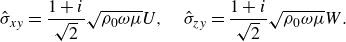 \begin{align} \hat {\sigma }_{xy}=\frac {1+i}{\sqrt {2}}\sqrt {\rho _0 \omega \mu } U,\quad \hat {\sigma }_{zy}=\frac {1+i}{\sqrt {2}}\sqrt {\rho _0 \omega \mu }W. \end{align}
Introducing the Reynolds number
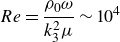 \begin{align} Re=\frac {\rho _0\omega }{k_3^2\mu }\sim 10^4 \end{align}
and considering a single spatial mode in the representation (4.23) leads to the equation for the amplitude function of the vertical velocity at the $m$
th mode in dimensionless form:
$m$
th mode in dimensionless form:
 \begin{equation} \begin{array}{c} W_m^{IV}-2\dfrac {m^2}{n^2}W_m^{\prime\prime}+\dfrac {m^4}{n^4}W_m=-\,i{Re}\left [(1+s)W_m^{\prime\prime}+\left (\dfrac {2}{\alpha ^2 }{\tilde {N}}^2 -1 -s\right )\dfrac {m^2}{n^2}W_m\right ]. \end{array} \end{equation}
The system contains two dimensionless dissipation coefficients, the normalised Stokes layer thickness $s$
and inverse Reynolds number
$s$
and inverse Reynolds number $ Re^{-1}$
, that represent the dissipation due to the wall friction and shear inside the pycnocline, respectively.
$ Re^{-1}$
, that represent the dissipation due to the wall friction and shear inside the pycnocline, respectively.
Equation (A5) with boundary conditions (4.35) is solved using the finite-difference method. The block-tridiagonal system of linear algebraic equations is obtained by the transformation of the fourth-order equation (A5) to a system of two second-order equations for $W_m$
and
$W_m$
and $\varOmega _m=W_m^{\prime\prime}$
.
$\varOmega _m=W_m^{\prime\prime}$
.


 Open access