


1. Introduction
The turbulent boundary layer (TBL) is among the most intriguing and important turbulent flows, drawing numerous researchers to engage in both physical and mathematical modelling of this phenomenon (Bradshaw Reference Bradshaw1977; Duan et al. Reference Duan, Beekman and Martin2010; Pirozzoli Reference Pirozzoli2011; Smits et al. Reference Smits, McKeon and Marusic2011; Marusic & Monty Reference Marusic and Monty2019; Chen et al. Reference Chen, Cheng, Gan and Fu2023; Cheng & Fu Reference Cheng and Fu2024). It is well known that incompressible TBLs at high Reynolds numbers exhibit several nearly universal scaling laws (van Driest Reference van Driest1951; Nagib et al. Reference Nagib, Chauhan and Monkewitz2007; Marusic et al. Reference Marusic, Monty, Hultmark and Smits2013; Chen & Sreenivasan Reference Chen and Sreenivasan2021). For example, the mean streamwise velocity profiles versus the wall-normal coordinate can be unified into the law of the wall through the non-dimensionalisation with respect to the friction velocity and kinematic viscosity. The skin-friction coefficient $C_f$
decreases along the streamwise direction, and is widely recognised to exhibit a functional relation with the Reynolds number
$C_f$
decreases along the streamwise direction, and is widely recognised to exhibit a functional relation with the Reynolds number $Re_\theta$
based on the momentum thickness
$Re_\theta$
based on the momentum thickness $\theta$
. The scaling law between
$\theta$
. The scaling law between $C_f$
and
$C_f$
and $Re_\theta$
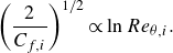
for incompressible TBLs over a flat plate can be expressed as (Nagib et al. Reference Nagib, Chauhan and Monkewitz2007)
$Re_\theta$
for incompressible TBLs over a flat plate can be expressed as (Nagib et al. Reference Nagib, Chauhan and Monkewitz2007)
 \begin{equation} \left (\frac{2}{C_f}\right )^{1/2}\propto \ln Re_{\theta }, \end{equation}
as a result of the logarithmic law of the mean streamwise velocity.
However, the compressible TBLs with high free-stream Mach number and non-negligible heat transfer do not directly obey the above scaling laws observed in incompressible cases. Consequently, significant efforts are dedicated to mapping compressible TBLs onto the incompressible counterparts by considering variations in mean properties such as density and viscosity inspired by Morkovin hypothesis (Bradshaw Reference Bradshaw1977). Such a transformation holds not only theoretical significance but also practical importance for reduced-order turbulence modelling, since it would enable the established incompressible wall models to be seamlessly applied to compressible flows (Chen et al. Reference Chen, Gan and Fu2024). An exemplary instance of the mapping is the velocity transformation. Over the past decades, several variants have been proposed for the velocity transformation of compressible TBLs (Zhang et al. Reference Zhang, Bi, Hussain, Li and She2012; Trettel & Larsson Reference Trettel and Larsson2016; Volpiani et al. Reference Volpiani, Iyer, Pirozzoli and Larsson2020b ; Griffin et al. Reference Griffin, Fu and Moin2021; Hasan et al. Reference Hasan, Larsson, Pirozzoli and Pecnik2023), building upon the pioneering work of van Driest (Reference van Driest1951). Among these methods, the physics-based Griffin-Fu-Moin (GFM) transformation (Griffin et al. Reference Griffin, Fu and Moin2021) combining the modified transformation of Zhang et al. (Reference Zhang, Bi, Hussain, Li and She2012) with the transformation of Trettel & Larsson (Reference Trettel and Larsson2016) successfully collapses mean streamwise velocity profiles of compressible TBLs with and without heat transfer into the law of the wall observed in incompressible scenarios.
In the field of aerospace engineering, it is essential to predict $C_f$
on a surface where high-speed airflow passes along with intense heat transfer. To this end, there are approximately 30 published theories for calculation of
$C_f$
on a surface where high-speed airflow passes along with intense heat transfer. To this end, there are approximately 30 published theories for calculation of $C_f$
of compressible TBLs (Spalding & Chi Reference Spalding and Chi1963). The theories presented by van Driest (Reference van Driest1951) and Spalding & Chi (Reference Spalding and Chi1964) exhibit lowest root mean square error, and are two of the most commonly used models to estimate
$C_f$
of compressible TBLs (Spalding & Chi Reference Spalding and Chi1963). The theories presented by van Driest (Reference van Driest1951) and Spalding & Chi (Reference Spalding and Chi1964) exhibit lowest root mean square error, and are two of the most commonly used models to estimate $C_f$
. Specifically, considering variations in density and viscosity, van Driest (Reference van Driest1951) introduced a scaling of
$C_f$
. Specifically, considering variations in density and viscosity, van Driest (Reference van Driest1951) introduced a scaling of $C_f$
with Reynolds number for compressible TBLs, which can be reduced to the incompressible relation as the Mach number approaches zero and the heat transfer becomes negligible. According to Spalding & Chi (Reference Spalding and Chi1964), the compressible scaling of
$C_f$
with Reynolds number for compressible TBLs, which can be reduced to the incompressible relation as the Mach number approaches zero and the heat transfer becomes negligible. According to Spalding & Chi (Reference Spalding and Chi1964), the compressible scaling of $C_f$
can be mapped to the incompressible relation by multiplying
$C_f$
can be mapped to the incompressible relation by multiplying $C_f$
and
$C_f$
and $Re_{\theta }$
by
$Re_{\theta }$
by $F_C$
and
$F_C$
and $F_{\theta }$
, respectively. Here,
$F_{\theta }$
, respectively. Here, $F_C$
and
$F_C$
and $F_{\theta }$
are functions of free-stream Mach number
$F_{\theta }$
are functions of free-stream Mach number $Ma_\infty$
and temperature
$Ma_\infty$
and temperature $T$
. Spalding & Chi (Reference Spalding and Chi1964) formulated
$T$
. Spalding & Chi (Reference Spalding and Chi1964) formulated $F_C$
and
$F_C$
and $F_{\theta }$
based on the theory of van Driest (Reference van Driest1951), called the van Driest II (vD-II) transformation. Moreover, an empirically modified
$F_{\theta }$
based on the theory of van Driest (Reference van Driest1951), called the van Driest II (vD-II) transformation. Moreover, an empirically modified $F_{\theta }$
using
$F_{\theta }$
using $C_f$
data in the presence of heat transfer is proposed as the Spalding–Chi (SC) transformation (Spalding & Chi Reference Spalding and Chi1964). Hopkins & Inouye (Reference Hopkins and Inouye1971) compared the performance of the above two transformations, and concluded that neither theory provided accurate predictions of
$C_f$
data in the presence of heat transfer is proposed as the Spalding–Chi (SC) transformation (Spalding & Chi Reference Spalding and Chi1964). Hopkins & Inouye (Reference Hopkins and Inouye1971) compared the performance of the above two transformations, and concluded that neither theory provided accurate predictions of $C_f$
for problems with wall-to-recovery temperature ratios below
$C_f$
for problems with wall-to-recovery temperature ratios below $0.3$
. The review by Bradshaw (Reference Bradshaw1977) further remarked that these two theories failed to predict
$0.3$
. The review by Bradshaw (Reference Bradshaw1977) further remarked that these two theories failed to predict $C_f$
on a very cold wall. In a more recent study, Huang et al. (Reference Huang, Duan and Choudhari2022) confirmed that neither of the two theories could map the compressible scaling of
$C_f$
on a very cold wall. In a more recent study, Huang et al. (Reference Huang, Duan and Choudhari2022) confirmed that neither of the two theories could map the compressible scaling of $C_f$
to incompressible relation for a highly cooled wall.
$C_f$
to incompressible relation for a highly cooled wall.
Based on the aforementioned discussions, none of the theories could consistently predict the $C_f$
of compressible TBLs with and without heat transfer. To this end, we revisit the theory of van Driest (Reference van Driest1951), and introduce a novel transformation for
$C_f$
of compressible TBLs with and without heat transfer. To this end, we revisit the theory of van Driest (Reference van Driest1951), and introduce a novel transformation for $C_f$
in this work. This proposed approach effectively maps the scaling law of
$C_f$
in this work. This proposed approach effectively maps the scaling law of $C_f$
for high-speed TBLs in air described by the ideal gas law, particularly those involving highly cooled walls, to the incompressible relation (i.e. (1.1)).
$C_f$
for high-speed TBLs in air described by the ideal gas law, particularly those involving highly cooled walls, to the incompressible relation (i.e. (1.1)).
2. Scaling law of $\boldsymbol{C}_\boldsymbol{f}$
for compressible TBLs over a flat plate
$\boldsymbol{C}_\boldsymbol{f}$
for compressible TBLs over a flat plate

The skin-friction coefficient, defined as $C_f=2\tau _w/\rho _\infty u_\infty ^2$
with wall shear stress
$C_f=2\tau _w/\rho _\infty u_\infty ^2$
with wall shear stress $\tau _w=\overline {\mu }\,\text{d}\overline {u}/\text{d}y|_w$
, free-stream density
$\tau _w=\overline {\mu }\,\text{d}\overline {u}/\text{d}y|_w$
, free-stream density $\rho _\infty$
, free-stream velocity
$\rho _\infty$
, free-stream velocity $u_\infty$
, viscosity
$u_\infty$
, viscosity $\overline {\mu }$
and wall-normal coordinate
$\overline {\mu }$
and wall-normal coordinate $y$
, is a crucial parameter in the design of supersonic and hypersonic aircraft. Hereafter, an overline denotes the Reynolds average, and subscripts
$y$
, is a crucial parameter in the design of supersonic and hypersonic aircraft. Hereafter, an overline denotes the Reynolds average, and subscripts $w$
and
$w$
and $\infty$
represent quantities at the wall and in the free stream, respectively. Coefficient
$\infty$
represent quantities at the wall and in the free stream, respectively. Coefficient $C_f$
is widely recognised to exhibit a functional relation with the Reynolds number
$C_f$
is widely recognised to exhibit a functional relation with the Reynolds number $Re_\theta =\rho _\infty u_\infty \theta /\mu _\infty$
based on the momentum thickness
$Re_\theta =\rho _\infty u_\infty \theta /\mu _\infty$
based on the momentum thickness $\theta$
. According to Spalding & Chi (Reference Spalding and Chi1964), for compressible TBLs over a flat plate,
$\theta$
. According to Spalding & Chi (Reference Spalding and Chi1964), for compressible TBLs over a flat plate, $C_f$
and
$C_f$
and $Re_\theta$
can be linearly transformed to
$Re_\theta$
can be linearly transformed to $C_{f,i}$
and
$C_{f,i}$
and $Re_{\theta ,i}$
by multiplying by
$Re_{\theta ,i}$
by multiplying by $F_C$
and
$F_C$
and $F_\theta$
, respectively, i.e.
$F_\theta$
, respectively, i.e.
 \begin{equation} C_{f,i}=F_C C_f,\quad Re_{\theta ,i}=F_\theta\, Re_\theta . \end{equation}
Here, $C_{f,i}$
and
$C_{f,i}$
and $Re_{\theta ,i}$
should obey the incompressible scaling for
$Re_{\theta ,i}$
should obey the incompressible scaling for $C_f$
, i.e. (1.1). The transformation factor
$C_f$
, i.e. (1.1). The transformation factor $F_C$
is the same in both vD-II (van Driest Reference van Driest1951) and SC (Spalding & Chi Reference Spalding and Chi1964) theories considering variations in density and viscosity, and can be expressed as
$F_C$
is the same in both vD-II (van Driest Reference van Driest1951) and SC (Spalding & Chi Reference Spalding and Chi1964) theories considering variations in density and viscosity, and can be expressed as
 \begin{equation} (F_C)_{{vD}} = (F_C)_{{SC}} = \left [\int _0^1 \sqrt {\frac {\overline {\rho }}{\rho _\infty }}\,\text{d}z\right ]^{-2}, \end{equation}
with $z=\overline {u}/u_\infty$
, density
$z=\overline {u}/u_\infty$
, density $\overline {\rho }$
and streamwise velocity
$\overline {\rho }$
and streamwise velocity $\overline {u}$
. Here, subscripts ‘vD’ and ‘SC’ refer to the transformation factors from the vD-II and SC theories, respectively. Using the fact that the pressure is nearly constant in TBLs and the velocity–temperature relation, the factor
$\overline {u}$
. Here, subscripts ‘vD’ and ‘SC’ refer to the transformation factors from the vD-II and SC theories, respectively. Using the fact that the pressure is nearly constant in TBLs and the velocity–temperature relation, the factor $F_C$
can be further written as
$F_C$
can be further written as
 \begin{equation} (F_C)_{{vD}} = (F_C)_{{SC}} = \dfrac {\dfrac{T_r}{T_\infty}-1}{\left (\sin ^{-1}\alpha +\sin ^{-1}\beta \right )^2}, \end{equation}
where $\alpha =(2A^2-B)/(B^2+4A^2)^{1/2}$
,
$\alpha =(2A^2-B)/(B^2+4A^2)^{1/2}$
, $\beta =B/(B^2+4A^2)^{1/2}$
,
$\beta =B/(B^2+4A^2)^{1/2}$
, $A=[r(\gamma -1)/2\times Ma_\infty ^2\,T_\infty /T_w]^{1/2}$
and
$A=[r(\gamma -1)/2\times Ma_\infty ^2\,T_\infty /T_w]^{1/2}$
and $B=T_r/T_w-1$
. Here,
$B=T_r/T_w-1$
. Here, $r$
is the recovery factor,
$r$
is the recovery factor, $T_r$
is the recovery temperature, and
$T_r$
is the recovery temperature, and $\gamma$
is the heat capacity ratio. However, the factor
$\gamma$
is the heat capacity ratio. However, the factor $F_\theta$
differs between the two theories and is given as
$F_\theta$
differs between the two theories and is given as
 \begin{equation} (F_\theta )_{{vD}} = \dfrac {\mu _\infty }{\mu _w}, \quad (F_\theta )_{{SC}} = \left (\dfrac {T_\infty }{T_w}\right )^{0.702}\left (\dfrac {T_r}{T_w}\right )^{0.772}. \end{equation}
These two transformations are used most commonly but fail to predict $C_f$
on a highly cooled wall (Hopkins & Inouye Reference Hopkins and Inouye1971; Bradshaw Reference Bradshaw1977; Huang et al. Reference Huang, Duan and Choudhari2022). The key issue with these two theories is the use of a linear transformation to eliminate the influences of Mach number and heat transfer on
$C_f$
on a highly cooled wall (Hopkins & Inouye Reference Hopkins and Inouye1971; Bradshaw Reference Bradshaw1977; Huang et al. Reference Huang, Duan and Choudhari2022). The key issue with these two theories is the use of a linear transformation to eliminate the influences of Mach number and heat transfer on $Re_\theta$
. Indeed, the momentum thickness is defined as
$Re_\theta$
. Indeed, the momentum thickness is defined as
 \begin{equation} \theta = \int _0^{\delta _e}\frac {\overline {\rho }}{\rho _\infty }\frac {\overline {u}}{u_\infty }\left (1-\frac {\overline {u}}{u_\infty }\right )\text{d}y, \end{equation}
where $\delta _e$
represents the TBL edge, typically chosen at the location where
$\delta _e$
represents the TBL edge, typically chosen at the location where $\overline {u}=0.99u_\infty$
. It is evident that the integrand in the definition of
$\overline {u}=0.99u_\infty$
. It is evident that the integrand in the definition of $\theta$
is a quadratic function of the velocity profile. Hence the factor
$\theta$
is a quadratic function of the velocity profile. Hence the factor $F_\theta$
in the linear transformation of (2.1) is unavailable to include all effects of Mach number and heat transfer on
$F_\theta$
in the linear transformation of (2.1) is unavailable to include all effects of Mach number and heat transfer on $\overline {u}$
. To address this concern, we redefine a momentum thickness
$\overline {u}$
. To address this concern, we redefine a momentum thickness $\theta ^*$
as
$\theta ^*$
as
 \begin{equation} \theta ^* = \int _0^{\delta _e}\frac {\overline {\rho }}{\rho _\infty }\frac {\overline {U}_I}{U_{I,\infty }}\left (1-\frac {\overline {U}_I}{U_{I,\infty }}\right )\text{d}(y^*\delta _v), \end{equation}
where $\delta _e$
is determined at
$\delta _e$
is determined at $\overline {U}_I=0.99U_{I,\infty }$
, the semi-local wall-normal coordinate is
$\overline {U}_I=0.99U_{I,\infty }$
, the semi-local wall-normal coordinate is $y^*=y\sqrt {\tau _w\overline {\rho }}/\overline {\mu }$
, the viscous length scale is
$y^*=y\sqrt {\tau _w\overline {\rho }}/\overline {\mu }$
, the viscous length scale is $\delta _v=\mu _w/\sqrt {\tau _w\rho _w}$
, and
$\delta _v=\mu _w/\sqrt {\tau _w\rho _w}$
, and $\overline {U}_I$
using the physics-based GFM velocity transformation (Griffin et al. Reference Griffin, Fu and Moin2021) is given as
$\overline {U}_I$
using the physics-based GFM velocity transformation (Griffin et al. Reference Griffin, Fu and Moin2021) is given as
 \begin{equation} \overline {U}_I = \int _0^{y^*}\frac {\dfrac{1}{\overline {\mu }^+} \dfrac{\text{d}\overline {U}^+}{\text{d}y^*}}{1 + \dfrac{1}{\overline {\mu }^+}\dfrac{\text{d}\overline {U}^+}{\text{d}y^*} - \overline {\mu }^+ \dfrac{\text{d}\overline {U}^+}{\text{d}y^+}}\,\text{d}y^*. \end{equation}
Throughout this paper, the superscript $+$
indicates a non-dimensionalisation by the friction velocity
$+$
indicates a non-dimensionalisation by the friction velocity $u_\tau =\sqrt {\tau _w/\rho _w}$
,
$u_\tau =\sqrt {\tau _w/\rho _w}$
, $\delta _v$
and
$\delta _v$
and $\mu _w$
. Note that
$\mu _w$
. Note that $\overline {U}_I$
in (2.7) is based on constant-stress-layer GFM transformation. In fact, the performances of
$\overline {U}_I$
in (2.7) is based on constant-stress-layer GFM transformation. In fact, the performances of $\overline {U}_I$
based on total-stress-based GFM transformation without the constant-stress-layer assumption, and on constant-stress-layer GFM transformation, are nearly identical (Griffin et al. Reference Griffin, Fu and Moin2021). Therefore, the constant-stress-layer assumption in (2.7) does not impact the establishment of the skin-friction scaling law, which has also been validated in Appendix A. The profiles of the transformed
$\overline {U}_I$
based on total-stress-based GFM transformation without the constant-stress-layer assumption, and on constant-stress-layer GFM transformation, are nearly identical (Griffin et al. Reference Griffin, Fu and Moin2021). Therefore, the constant-stress-layer assumption in (2.7) does not impact the establishment of the skin-friction scaling law, which has also been validated in Appendix A. The profiles of the transformed $\overline {U}_I(y^*)$
in compressible TBLs, with and without heat transfer, collapse to the incompressible law of the wall, and are independent of Mach number and heat transfer. Clearly,
$\overline {U}_I(y^*)$
in compressible TBLs, with and without heat transfer, collapse to the incompressible law of the wall, and are independent of Mach number and heat transfer. Clearly, $\theta ^*$
is similar to the traditional momentum thickness
$\theta ^*$
is similar to the traditional momentum thickness $\theta$
, except that
$\theta$
, except that $\theta ^*$
is based on
$\theta ^*$
is based on $\overline {U}_I$
and
$\overline {U}_I$
and $y^*$
. Since the profiles of
$y^*$
. Since the profiles of $\overline {U}_I(y^*)$
are independent of Mach number and heat transfer,
$\overline {U}_I(y^*)$
are independent of Mach number and heat transfer, $\theta ^*$
can be physically interpreted as a momentum thickness unaffected by the effects of Mach number and heat transfer in the velocity profiles of compressible TBLs. Therefore, only
$\theta ^*$
can be physically interpreted as a momentum thickness unaffected by the effects of Mach number and heat transfer in the velocity profiles of compressible TBLs. Therefore, only $\overline {\rho }$
in the redefined
$\overline {\rho }$
in the redefined $\theta ^*$
is affected by Mach number and heat transfer. These effects can be reasonably included in a linear transformation factor
$\theta ^*$
is affected by Mach number and heat transfer. These effects can be reasonably included in a linear transformation factor $F_{\theta ^*}$
with a redefined Reynolds number
$F_{\theta ^*}$
with a redefined Reynolds number $Re_{\theta ^*}=\rho _\infty u_\infty \theta ^*/\mu _\infty$
. It is important to highlight that by multiplying
$Re_{\theta ^*}=\rho _\infty u_\infty \theta ^*/\mu _\infty$
. It is important to highlight that by multiplying $y^*$
by
$y^*$
by $\delta _v$
in (2.6),
$\delta _v$
in (2.6), $Re_{\theta ^*}$
can be precisely reduced to the
$Re_{\theta ^*}$
can be precisely reduced to the $Re_{\theta }$
of the incompressible case, where
$Re_{\theta }$
of the incompressible case, where $\overline {\rho }$
and
$\overline {\rho }$
and $\overline {\mu }$
are nearly constant.
$\overline {\mu }$
are nearly constant.
Subsequently, we will theoretically derive the scaling law for $C_f$
based on
$C_f$
based on $Re_{\theta ^*}$
. Given the fact that the contribution of the integrand to
$Re_{\theta ^*}$
. Given the fact that the contribution of the integrand to $\theta ^*$
in both the viscous sublayer (
$\theta ^*$
in both the viscous sublayer ( $\overline {U}_I/U_{I,\infty} \rightarrow 0$
) and outer layer (
$\overline {U}_I/U_{I,\infty} \rightarrow 0$
) and outer layer ( $\overline {U}_I/U_{I,\infty} \rightarrow 1$
) is negligible, the log-law behaviour of
$\overline {U}_I/U_{I,\infty} \rightarrow 1$
) is negligible, the log-law behaviour of $\overline {U}_I$
, expressed as
$\overline {U}_I$
, expressed as
 \begin{equation} y^* = \dfrac{\exp (\kappa \overline {U}_I)}{E}, \end{equation}
is suitably employed to approximate $\theta ^*$
. Here,
$\theta ^*$
. Here, $\kappa$
is the von Kármán constant, and
$\kappa$
is the von Kármán constant, and $E$
is a constant. By substituting (2.8) into (2.6), one can obtain
$E$
is a constant. By substituting (2.8) into (2.6), one can obtain
 \begin{equation} \theta ^* = \frac {\kappa }{E}\delta _vU_{I,\infty }\int _0^1\frac {\overline {\rho }}{\rho _\infty }Z(1-Z)\exp (\kappa U_{I,\infty }Z)\,\text{d}Z, \end{equation}
where $Z=\overline {U}_I/U_{I,\infty }$
. The integral term in above equation,
$Z=\overline {U}_I/U_{I,\infty }$
. The integral term in above equation, $\int _0^1(\overline {\rho }/\rho _\infty) Z(1-Z){} \!\exp(\kappa U_{I,\infty }Z)\,\text{d}Z = 1/(\kappa U_{I,\infty })\int _0^1(\overline {\rho }/\rho _\infty) Z(1-Z)\,\text{d}\exp (\kappa U_{I,\infty }Z)$
, can be integrated by parts and expressed as
$\int _0^1(\overline {\rho }/\rho _\infty) Z(1-Z){} \!\exp(\kappa U_{I,\infty }Z)\,\text{d}Z = 1/(\kappa U_{I,\infty })\int _0^1(\overline {\rho }/\rho _\infty) Z(1-Z)\,\text{d}\exp (\kappa U_{I,\infty }Z)$
, can be integrated by parts and expressed as
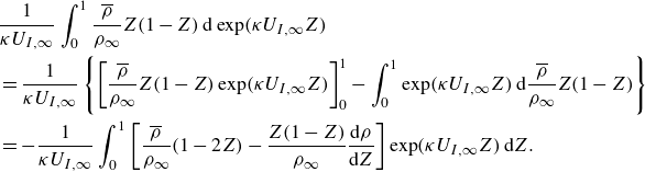 \begin{align} & \frac {1}{\kappa U_{I,\infty }}\int _0^1\frac {\overline {\rho }}{\rho _\infty } Z(1-Z)\,\text{d}\exp (\kappa U_{I,\infty }Z) \notag \\ & =\frac {1}{\kappa U_{I,\infty }}\left \lbrace \left [\frac {\overline {\rho }}{\rho _\infty } Z(1-Z)\exp (\kappa U_{I,\infty }Z)\right ]_0^1- \int _0^1\exp (\kappa U_{I,\infty }Z)\,\text{d}\frac {\overline {\rho }}{\rho _\infty } Z(1-Z)\right \rbrace \notag \\ & =-\frac {1}{\kappa U_{I,\infty }}\int _0^1\left [\frac {\overline {\rho }}{\rho _\infty } (1-2Z)-\frac {Z(1-Z)}{\rho _\infty }\frac {\text{d}\rho }{\text{d}Z} \right ] \exp (\kappa U_{I,\infty }Z)\,\text{d}Z. \end{align}
Here, the term $ \bigl[{(\overline {\rho }}/{\rho _\infty }) Z(1-Z)\exp (\kappa U_{I,\infty }Z) \bigr]_0^1$
represents the difference in values of
$ \bigl[{(\overline {\rho }}/{\rho _\infty }) Z(1-Z)\exp (\kappa U_{I,\infty }Z) \bigr]_0^1$
represents the difference in values of $ [({\overline {\rho }}/{\rho _\infty }) Z(1-Z)\exp (\kappa U_{I,\infty }Z) ]$
at the locations
$ [({\overline {\rho }}/{\rho _\infty }) Z(1-Z)\exp (\kappa U_{I,\infty }Z) ]$
at the locations $Z=1$
and
$Z=1$
and $Z=0$
. Similarly, by repeatedly applying integration by parts to (2.10), (2.9) can be expressed as an asymptotic series of
$Z=0$
. Similarly, by repeatedly applying integration by parts to (2.10), (2.9) can be expressed as an asymptotic series of $1/\kappa U_{I,\infty }$
as
$1/\kappa U_{I,\infty }$
as
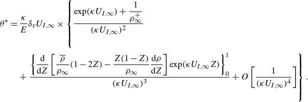 \begin{align} \theta ^* &= \frac {\kappa }{E}\delta _vU_{I,\infty } \times\left \lbrace \frac {\exp (\kappa U_{I,\infty })+ \dfrac{1}{\rho _\infty ^+}}{(\kappa U_{I,\infty })^2} \vphantom{\frac {\left \lbrace \dfrac {\text{d}}{\text{d}Z}\left [\dfrac {\overline {\rho }}{\rho _\infty } (1-2Z)-\dfrac {Z(1-Z)}{\rho _\infty }\dfrac {\text{d}\rho }{\text{d}Z} \right ] \exp (\kappa U_{I,\infty }Z)\right \rbrace _0^1 }{\left \lbrace \dfrac {\text{d}}{\text{d}Z}\left [\dfrac {\overline {\rho }}{\rho _\infty } (1-2Z)-\dfrac {Z(1-Z)}{\rho _\infty }\dfrac {\text{d}\rho }{\text{d}Z} \right ] \exp (\kappa U_{I,\infty }Z)\right \rbrace _0^1 }} \right . \notag \\&\quad + \left . \frac {\left \lbrace \dfrac {\text{d}}{\text{d}Z}\left [\dfrac {\overline {\rho }}{\rho _\infty } (1-2Z)-\dfrac {Z(1-Z)}{\rho _\infty }\dfrac {\text{d}\rho }{\text{d}Z} \right ] \exp (\kappa U_{I,\infty }Z)\right \rbrace _0^1 }{(\kappa U_{I,\infty })^3} + O\left [\frac {1}{(\kappa U_{I,\infty })^4}\right ]\right \rbrace . \end{align}
According to the logarithmic law of TBLs, it can be estimated that $U_{I,\infty }\gtrsim 20$
, leading to
$U_{I,\infty }\gtrsim 20$
, leading to $\kappa U_{I,\infty }$
being of the order of
$\kappa U_{I,\infty }$
being of the order of $O(10)$
for TBLs. The ratio of magnitude of the third-order term related to
$O(10)$
for TBLs. The ratio of magnitude of the third-order term related to $1/(\kappa U_{I,\infty })^3$
to the magnitude of the second-order term related to
$1/(\kappa U_{I,\infty })^3$
to the magnitude of the second-order term related to $1/(\kappa U_{I,\infty })^2$
is of the order of
$1/(\kappa U_{I,\infty })^2$
is of the order of $O(10^{-1})$
. Moreover, given the fact that pressure is nearly constant in TBLs,
$O(10^{-1})$
. Moreover, given the fact that pressure is nearly constant in TBLs, $1/\rho _\infty ^+\approx T_\infty /T_w$
. For common high-speed TBLs,
$1/\rho _\infty ^+\approx T_\infty /T_w$
. For common high-speed TBLs, $T_\infty /T_w \lt 1$
, which implies
$T_\infty /T_w \lt 1$
, which implies $1/\rho _\infty ^+\lt 1\ll \exp (\kappa U_{I,\infty })\sim O(10^4)$
. To this end, the term
$1/\rho _\infty ^+\lt 1\ll \exp (\kappa U_{I,\infty })\sim O(10^4)$
. To this end, the term $1/\rho _\infty ^+$
, which is much smaller than
$1/\rho _\infty ^+$
, which is much smaller than $\exp (\kappa U_{I,\infty })$
, along with the higher-order terms that are smaller than the second-order term, can be neglected. Consequently,
$\exp (\kappa U_{I,\infty })$
, along with the higher-order terms that are smaller than the second-order term, can be neglected. Consequently, $Re_{\theta ^*}$
can be determined by
$Re_{\theta ^*}$
can be determined by
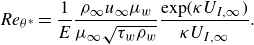 \begin{equation} Re_{\theta ^*} = \frac {1}{E}\frac {\rho _\infty u_\infty \mu _w}{\mu _\infty \sqrt {\tau _w\rho _w}}\frac {\exp (\kappa U_{I,\infty })}{\kappa U_{I,\infty }}. \end{equation}
Moreover, according to (2.7), $U_{I,\infty }$
is determined by
$U_{I,\infty }$
is determined by
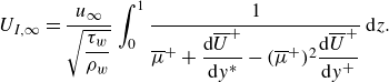 \begin{equation} U_{I,\infty } = \frac {u_\infty }{\sqrt {\dfrac{\tau _w}{\rho _w}}}\int _0^1\frac {1}{\overline {\mu }^+ + \dfrac{\text{d}\overline {U}^+}{\text{d}y^*} -(\overline {\mu }^+)^2 \dfrac{\text{d}\overline {U}^+}{\text{d}y^+}}\,\text{d}z. \end{equation}
Letting $F=\int _0^1[\overline {\mu }^++\text{d}\overline {U}^+/\text{d}y^*-(\overline {\mu }^+)^2\,\text{d}\overline {U}^+/\text{d}y^+]^{-1}\,\text{d}z$
, which is determined by given viscosity and velocity profiles in TBLs, the functional relation between
$F=\int _0^1[\overline {\mu }^++\text{d}\overline {U}^+/\text{d}y^*-(\overline {\mu }^+)^2\,\text{d}\overline {U}^+/\text{d}y^+]^{-1}\,\text{d}z$
, which is determined by given viscosity and velocity profiles in TBLs, the functional relation between $Re_{\theta ^*}$
and
$Re_{\theta ^*}$
and $C_f$
can be obtained by substituting (2.13) into (2.12) as
$C_f$
can be obtained by substituting (2.13) into (2.12) as
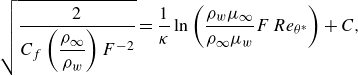 \begin{equation} \sqrt {\frac {2}{C_f \left(\dfrac{\rho _\infty }{\rho _w} \right)F^{-2}}} = \frac {1}{\kappa }\ln \left ( \frac {\rho _w\mu _\infty }{\rho _\infty \mu _w}F\,Re_{\theta ^*}\right ) + C, \end{equation}
with a constant $C=\ln (E\kappa )/\kappa$
. Obviously, we can define a novel transformation for
$C=\ln (E\kappa )/\kappa$
. Obviously, we can define a novel transformation for $C_f$
and
$C_f$
and $Re_{\theta ^*}$
as
$Re_{\theta ^*}$
as
 \begin{equation} C_{f,i}=F_{C^*} C_f,\quad Re_{\theta ,i}=F_{\theta ^*}\, Re_{\theta ^*}, \end{equation}
where the new transformation factors are expressed as
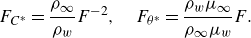 \begin{equation} F_{C^*}=\frac {\rho _\infty }{\rho _w}F^{-2},\quad F_{\theta ^*}= \frac {\rho _w\mu _\infty }{\rho _\infty \mu _w}F. \end{equation}
Employing the present transformation, i.e. (2.15), the scaling for $C_f$
of a compressible TBL can be written as
$C_f$
of a compressible TBL can be written as
 \begin{equation} \left (\dfrac{2}{C_{f,i}}\right )^{1/2} \propto \ln Re_{\theta ,i}. \end{equation}
The functional relation between the newly transformed $C_{f,i}$
and
$C_{f,i}$
and $Re_{\theta ,i}$
is exactly the same as the incompressible scaling for
$Re_{\theta ,i}$
is exactly the same as the incompressible scaling for $C_f$
expressed by (1.1). Furthermore, in the incompressible TBL with constant
$C_f$
expressed by (1.1). Furthermore, in the incompressible TBL with constant $\overline {\rho }$
and
$\overline {\rho }$
and $\overline {\mu }$
, it is clear that
$\overline {\mu }$
, it is clear that $F_{C^*}=1$
,
$F_{C^*}=1$
, $F_{\theta ^*}=1$
and
$F_{\theta ^*}=1$
and $Re_{\theta ^*}=Re_{\theta }$
. Hence the newly transformed
$Re_{\theta ^*}=Re_{\theta }$
. Hence the newly transformed $C_{f,i}$
and
$C_{f,i}$
and $Re_{\theta ,i}$
can be precisely reduced to the incompressible counterparts when the effects of Mach number and heat transfer are negligible. The preceding discussions on the innovative transformation indicate that this novel approach theoretically maps the scaling for
$Re_{\theta ,i}$
can be precisely reduced to the incompressible counterparts when the effects of Mach number and heat transfer are negligible. The preceding discussions on the innovative transformation indicate that this novel approach theoretically maps the scaling for $C_f$
of compressible TBLs for air described by the ideal gas law to the incompressible relation for
$C_f$
of compressible TBLs for air described by the ideal gas law to the incompressible relation for $C_f$
. Furthermore, by performing a linear fit of the data to determine the constants
$C_f$
. Furthermore, by performing a linear fit of the data to determine the constants $\kappa _f$
and
$\kappa _f$
and $C$
, the scaling for
$C$
, the scaling for $C_f$
of a compressible TBL can be quantified as
$C_f$
of a compressible TBL can be quantified as
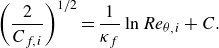 \begin{equation} \left (\dfrac{2}{C_{f,i}}\right )^{1/2} = \frac {1}{\kappa _f}\ln Re_{\theta ,i} + C. \end{equation}
Given the approximations involved in deriving the skin-friction scaling, the constant obtained by linearly fitting $ (2/C_{f,i} )^{1/2}$
and
$ (2/C_{f,i} )^{1/2}$
and $\ln Re_{\theta ,i}$
in (2.18) will differ from the value of the von Kármán constant
$\ln Re_{\theta ,i}$
in (2.18) will differ from the value of the von Kármán constant $\kappa$
obtained from the stream velocity profile, and is therefore denoted as
$\kappa$
obtained from the stream velocity profile, and is therefore denoted as $\kappa _f$
. Additionally, based on the definition of
$\kappa _f$
. Additionally, based on the definition of $Re_{\theta ^*}$
, the newly transformed
$Re_{\theta ^*}$
, the newly transformed $Re_{\theta ,i}$
can be further expressed as
$Re_{\theta ,i}$
can be further expressed as $Re_{\theta ,i}=F\rho _w u_\infty \theta ^*/\mu _w$
. It is evident that
$Re_{\theta ,i}=F\rho _w u_\infty \theta ^*/\mu _w$
. It is evident that $\mu _\infty$
used in the present definition of
$\mu _\infty$
used in the present definition of $Re_{\theta ^*}$
does not appear in the final form of transformed
$Re_{\theta ^*}$
does not appear in the final form of transformed $Re_{\theta ,i}$
. In other words, in the definition of
$Re_{\theta ,i}$
. In other words, in the definition of $Re_{\theta ^*}$
, replacing
$Re_{\theta ^*}$
, replacing $\mu _\infty$
with
$\mu _\infty$
with $\mu _w$
, shear stress-weighted average viscosity introduced by Kianfar et al. (Reference Kianfar, Di Renzo, Williams, Elnahhas and Johnson2023) to account for the relative influence of turbulence on the skin friction, or any other viscosity, does not change the final form of the transformed
$\mu _w$
, shear stress-weighted average viscosity introduced by Kianfar et al. (Reference Kianfar, Di Renzo, Williams, Elnahhas and Johnson2023) to account for the relative influence of turbulence on the skin friction, or any other viscosity, does not change the final form of the transformed $Re_{\theta ,i}$
.
$Re_{\theta ,i}$
.
3. Validation of the newly proposed scaling law
To verify the scaling law for $C_f$
, we conduct direct numerical simulations (DNS) of compressible TBLs, and also collect as much published DNS data as possible on compressible TBLs with adiabatic (Li et al. Reference Li, Tong, Yu and Li2009; Pirozzoli & Bernardini Reference Pirozzoli and Bernardini2011; Volpiani et al. Reference Volpiani, Iyer, Pirozzoli and Larsson2018; Zhang et al. Reference Zhang, Wan, Liu, Sun and Lu2018, Reference Zhang, Wan, Sun and Lu2024; Maeyama & Kawai Reference Maeyama and Kawai2023; Cogo et al. Reference Cogo, Baù, Chinappi, Bernardini and Picano2023), cooled (Zhang et al. Reference Zhang, Wan, Liu, Sun and Lu2018, Reference Zhang, Wan, Sun and Lu2022; Li et al. Reference Li, Tong, Yu and Li2019; Volpiani et al. Reference Volpiani, Bernardini and Larsson2020a
; Cogo et al. Reference Cogo, Baù, Chinappi, Bernardini and Picano2023), and heated (Volpiani et al. Reference Volpiani, Bernardini and Larsson2018, Reference Volpiani, Bernardini and Larsson2020a
) walls. The data cover a fairly wide range of flow conditions, with
$C_f$
, we conduct direct numerical simulations (DNS) of compressible TBLs, and also collect as much published DNS data as possible on compressible TBLs with adiabatic (Li et al. Reference Li, Tong, Yu and Li2009; Pirozzoli & Bernardini Reference Pirozzoli and Bernardini2011; Volpiani et al. Reference Volpiani, Iyer, Pirozzoli and Larsson2018; Zhang et al. Reference Zhang, Wan, Liu, Sun and Lu2018, Reference Zhang, Wan, Sun and Lu2024; Maeyama & Kawai Reference Maeyama and Kawai2023; Cogo et al. Reference Cogo, Baù, Chinappi, Bernardini and Picano2023), cooled (Zhang et al. Reference Zhang, Wan, Liu, Sun and Lu2018, Reference Zhang, Wan, Sun and Lu2022; Li et al. Reference Li, Tong, Yu and Li2019; Volpiani et al. Reference Volpiani, Bernardini and Larsson2020a
; Cogo et al. Reference Cogo, Baù, Chinappi, Bernardini and Picano2023), and heated (Volpiani et al. Reference Volpiani, Bernardini and Larsson2018, Reference Volpiani, Bernardini and Larsson2020a
) walls. The data cover a fairly wide range of flow conditions, with $Ma_\infty$
ranging from
$Ma_\infty$
ranging from $0.5$
to
$0.5$
to $14$
, friction Reynolds number
$14$
, friction Reynolds number $Re_\tau$
ranging from
$Re_\tau$
ranging from $100$
to
$100$
to $2400$
, and
$2400$
, and $T_w/T_r$
ranging from
$T_w/T_r$
ranging from $0.15$
to
$0.15$
to $1.9$
. A wall-to-recovery temperature ratio
$1.9$
. A wall-to-recovery temperature ratio $T_w/T_r$
less than
$T_w/T_r$
less than $1$
signifies a cooled wall,
$1$
signifies a cooled wall, $T_w/T_r$
equal to
$T_w/T_r$
equal to $1$
denotes an adiabatic wall, and
$1$
denotes an adiabatic wall, and $T_w/T_r$
greater than
$T_w/T_r$
greater than $1$
indicates a heated wall. Detailed parameters regarding the DNS data of TBLs can be found in tables 1, 2 and 3.
$1$
indicates a heated wall. Detailed parameters regarding the DNS data of TBLs can be found in tables 1, 2 and 3.
Table 1. The parameters for compressible TBLs self-simulated using the open-source code STREAmS (Bernardini et al. Reference Bernardini, Modesti, Salvadore and Pirozzoli2021, Reference Bernardini, Modesti, Salvadore, Sathyanarayana, Della Posta and Pirozzoli2023) in fully developed turbulent regions. Here, $Ma_\infty$
is the free-stream Mach number,
$Ma_\infty$
is the free-stream Mach number, $T_w/T_r$
is the wall-to-recovery temperature ratio,
$T_w/T_r$
is the wall-to-recovery temperature ratio, $Re_\tau$
is the friction Reynolds number,
$Re_\tau$
is the friction Reynolds number, $Re_{\delta _e}$
is the Reynolds number based on boundary layer thickness,
$Re_{\delta _e}$
is the Reynolds number based on boundary layer thickness, $Re_\theta$
is the Reynolds number based on momentum thickness, and
$Re_\theta$
is the Reynolds number based on momentum thickness, and $Re_{\theta ^*}$
is the redefined Reynolds number based on transformed momentum thickness.
$Re_{\theta ^*}$
is the redefined Reynolds number based on transformed momentum thickness.
Table 2. The parameters for compressible TBLs of Zhang et al. (Reference Zhang, Wan, Liu, Sun and Lu2022, Reference Zhang, Wan, Sun and Lu2024), Li et al. (Reference Li, Fu, Ma and Gao2009, Reference Li, Tong, Yu and Li2019) and Volpiani et al. (Reference Volpiani, Bernardini and Larsson2018, Reference Volpiani, Bernardini and Larsson2020a ) in fully developed turbulent regions. The representations of the parameters are presented in table 1.
Table 3. The parameters for compressible TBLs of Maeyama & Kawai (Reference Maeyama and Kawai2023), Zhang et al. (Reference Zhang, Duan and Choudhari2018), Cogo et al. (Reference Cogo, Baù, Chinappi, Bernardini and Picano2023) and Pirozzoli & Bernardini (Reference Pirozzoli and Bernardini2011) in fully developed turbulent regions. The representations of the parameters are presented in table 1.
Figure 1. The transformed $(2/C_{f,i})^{1/2}$
versus transformed
$(2/C_{f,i})^{1/2}$
versus transformed $Re_{\theta ,i}$
: (a) present theory (using (2.15)), (b) vD-II theory (using (2.1) with
$Re_{\theta ,i}$
: (a) present theory (using (2.15)), (b) vD-II theory (using (2.1) with $(F_C)_{{vD}}$
and
$(F_C)_{{vD}}$
and $(F_\theta )_{{vD}}$
) and (c) SC theory (using (2.1) with
$(F_\theta )_{{vD}}$
) and (c) SC theory (using (2.1) with $(F_C)_{{SC}}$
and
$(F_C)_{{SC}}$
and $(F_\theta )_{{SC}}$
). The coloured symbols represent DNS data from both adiabatic and diabatic compressible TBLs, with colours indicating the wall-to-recovery temperature ratios. The black symbols
$(F_\theta )_{{SC}}$
). The coloured symbols represent DNS data from both adiabatic and diabatic compressible TBLs, with colours indicating the wall-to-recovery temperature ratios. The black symbols $\times$
denote DNS and experimental data for incompressible TBLs, with
$\times$
denote DNS and experimental data for incompressible TBLs, with $Re_\theta \leqslant 3000$
from Schlatter & Örlü (Reference Schlatter and Örlü2010),
$Re_\theta \leqslant 3000$
from Schlatter & Örlü (Reference Schlatter and Örlü2010), $4000\leqslant Re_\theta \leqslant 6500$
from Sillero et al. (Reference Sillero, Jiménez and Moser2013), and
$4000\leqslant Re_\theta \leqslant 6500$
from Sillero et al. (Reference Sillero, Jiménez and Moser2013), and $13\,000\lt Re_\theta \lt 52\,000$
(corresponding to
$13\,000\lt Re_\theta \lt 52\,000$
(corresponding to $6000\lt Re_\tau \lt 20\,000$
) from Samie et al. (Reference Samie, Marusic, Hutchins, Fu, Fan, Hultmark and Smits2018). The dashed and dash-dotted lines represent the incompressible correlations of Coles–Fernholz (modified by Nagib et al. (Reference Nagib, Chauhan and Monkewitz2007), i.e.
$6000\lt Re_\tau \lt 20\,000$
) from Samie et al. (Reference Samie, Marusic, Hutchins, Fu, Fan, Hultmark and Smits2018). The dashed and dash-dotted lines represent the incompressible correlations of Coles–Fernholz (modified by Nagib et al. (Reference Nagib, Chauhan and Monkewitz2007), i.e. $(2/C_{f,i})^{1/2}_{{CF}}=2.604\ln Re_{\theta ,i}+4.127$
) and Smits et al. (Reference Smits, Matheson and Joubert1983) (i.e.
$(2/C_{f,i})^{1/2}_{{CF}}=2.604\ln Re_{\theta ,i}+4.127$
) and Smits et al. (Reference Smits, Matheson and Joubert1983) (i.e. $(C_{f,i})_{{SM}}=0.024\,Re_{\theta ,i}^{-1/4}$
), respectively. The squared Pearson correlation coefficient
$(C_{f,i})_{{SM}}=0.024\,Re_{\theta ,i}^{-1/4}$
), respectively. The squared Pearson correlation coefficient $R^2$
between
$R^2$
between $(2/C_{f,i})^{1/2}$
and
$(2/C_{f,i})^{1/2}$
and $\ln Re_{\theta ,i}$
for each transformation is provided in each plot. For a pair of variables
$\ln Re_{\theta ,i}$
for each transformation is provided in each plot. For a pair of variables $(X,Y)$
,
$(X,Y)$
, $R^2$
is defined as
$R^2$
is defined as $R^2 = \text{cov}^2(X,Y)/(\sigma _X^2\sigma _Y^2)$
, where
$R^2 = \text{cov}^2(X,Y)/(\sigma _X^2\sigma _Y^2)$
, where $\text{cov}$
denotes the covariance,
$\text{cov}$
denotes the covariance, $\sigma _X$
is the standard deviation of
$\sigma _X$
is the standard deviation of $X$
, and
$X$
, and $\sigma _Y$
is the standard deviation of
$\sigma _Y$
is the standard deviation of $Y$
.
$Y$
.
Figure 1(a) displays the correlation between the transformed $ (2/C_{f,i} )^{1/2}$
and
$ (2/C_{f,i} )^{1/2}$
and $Re_{\theta ,i}$
according to the proposed theory, employing logarithmic coordinate for
$Re_{\theta ,i}$
according to the proposed theory, employing logarithmic coordinate for $Re_{\theta ,i}$
. It should be noted that a second-order difference scheme is uniformly employed to calculate the derivatives in
$Re_{\theta ,i}$
. It should be noted that a second-order difference scheme is uniformly employed to calculate the derivatives in $F_{C^*}$
and
$F_{C^*}$
and $F_{\theta ^*}$
for all data. With a squared Pearson correlation coefficient
$F_{\theta ^*}$
for all data. With a squared Pearson correlation coefficient $R^2$
as high as
$R^2$
as high as $0.99$
between
$0.99$
between $ (2/C_{f,i} )^{1/2}$
and
$ (2/C_{f,i} )^{1/2}$
and $\ln Re_{\theta ,i}$
, it is indicated that the transformed
$\ln Re_{\theta ,i}$
, it is indicated that the transformed $C_{f,i}$
of compressible TBLs with and without heat transfer strictly satisfies the incompressible scaling for
$C_{f,i}$
of compressible TBLs with and without heat transfer strictly satisfies the incompressible scaling for $C_f$
, i.e.
$C_f$
, i.e. $ (2/C_{f,i} )^{1/2}\propto \ln Re_{\theta ,i}$
, based on present theory. For comparison, the results of vD-II and SC theories are depicted in figures 1(b) and 1(c), respectively. No significant linear relationship is observed between
$ (2/C_{f,i} )^{1/2}\propto \ln Re_{\theta ,i}$
, based on present theory. For comparison, the results of vD-II and SC theories are depicted in figures 1(b) and 1(c), respectively. No significant linear relationship is observed between $ (2/C_{f,i} )^{1/2}$
and
$ (2/C_{f,i} )^{1/2}$
and $\ln Re_{\theta ,i}$
under these two theories, with
$\ln Re_{\theta ,i}$
under these two theories, with $R^2$
values
$R^2$
values $0.85$
and
$0.85$
and $0.86$
, much less than
$0.86$
, much less than $0.99$
of present theory.
$0.99$
of present theory.
To quantitatively confirm if the present theory effectively collapses the compressible scaling for $C_f$
to the incompressible relation, the constants
$C_f$
to the incompressible relation, the constants $\kappa _f$
and
$\kappa _f$
and $C$
are determined by linearly fitting present data for compressible TBLs, and (2.18) is plotted in figure 1. Two commonly used incompressible correlations for
$C$
are determined by linearly fitting present data for compressible TBLs, and (2.18) is plotted in figure 1. Two commonly used incompressible correlations for $C_f$
, namely the modified Coles–Fernholz (Nagib et al. Reference Nagib, Chauhan and Monkewitz2007) and Smits et al. (Reference Smits, Matheson and Joubert1983) relations, are also depicted. It is evident that the
$C_f$
, namely the modified Coles–Fernholz (Nagib et al. Reference Nagib, Chauhan and Monkewitz2007) and Smits et al. (Reference Smits, Matheson and Joubert1983) relations, are also depicted. It is evident that the $C_{f,i}$
correlation of present theory lies between two incompressible relations at
$C_{f,i}$
correlation of present theory lies between two incompressible relations at $Re_{\theta ,i}\gtrsim 500$
. However, the
$Re_{\theta ,i}\gtrsim 500$
. However, the $C_{f,i}$
correlation of vD-II theory deviates from two incompressible relations at
$C_{f,i}$
correlation of vD-II theory deviates from two incompressible relations at $Re_{\theta ,i}\lesssim 10\,000$
, and that of SC theory notably deviates from incompressible relations. Moreover, the
$Re_{\theta ,i}\lesssim 10\,000$
, and that of SC theory notably deviates from incompressible relations. Moreover, the $C_f$
of incompressible DNS data (Schlatter & Örlü Reference Schlatter and Örlü2010; Sillero et al. Reference Sillero, Jiménez and Moser2013) and experimental data (Samie et al. Reference Samie, Marusic, Hutchins, Fu, Fan, Hultmark and Smits2018) also falls between two incompressible relations, following the
$C_f$
of incompressible DNS data (Schlatter & Örlü Reference Schlatter and Örlü2010; Sillero et al. Reference Sillero, Jiménez and Moser2013) and experimental data (Samie et al. Reference Samie, Marusic, Hutchins, Fu, Fan, Hultmark and Smits2018) also falls between two incompressible relations, following the $C_{f,i}$
correlation of present theory. Hence comparing with vD-II and SC theories, the present theory elegantly maps the compressible scaling for
$C_{f,i}$
correlation of present theory. Hence comparing with vD-II and SC theories, the present theory elegantly maps the compressible scaling for $C_f$
to the incompressible relation. Additionally, the performance of present theory for TBLs at supercritical pressure is discussed in Appendix B.
$C_f$
to the incompressible relation. Additionally, the performance of present theory for TBLs at supercritical pressure is discussed in Appendix B.
Figure 2. The error of the skin-friction coefficient, defined as $|(2/C_{f,i})^{1/2}_{{DNS}}-(2/C_{f,i})^{1/2}_{{CF}} |/(2/C_{f,i})^{1/2}_{{CF}}$
: (a) present theory, (b) vD-II theory, and (c) SC theory. The black dashed line in each plot represents the maximum error.
$|(2/C_{f,i})^{1/2}_{{DNS}}-(2/C_{f,i})^{1/2}_{{CF}} |/(2/C_{f,i})^{1/2}_{{CF}}$
: (a) present theory, (b) vD-II theory, and (c) SC theory. The black dashed line in each plot represents the maximum error.
Error statistics of $C_{f,i}$
from DNS data, compared to the modified Coles–Fernholz relation (Nagib et al. Reference Nagib, Chauhan and Monkewitz2007), are provided in figure 2 to assess the theory’s performance in predicting
$C_{f,i}$
from DNS data, compared to the modified Coles–Fernholz relation (Nagib et al. Reference Nagib, Chauhan and Monkewitz2007), are provided in figure 2 to assess the theory’s performance in predicting $C_f$
for compressible TBLs. The maximum errors for the present, vD-II and SC theories are slightly below
$C_f$
for compressible TBLs. The maximum errors for the present, vD-II and SC theories are slightly below $5\, \%$
, slightly below
$5\, \%$
, slightly below $10\, \%$
, and surpassing
$10\, \%$
, and surpassing $14\, \%$
, respectively. The data from compressible TBLs with heated and extensively cooled walls exhibit a significant error for vD-II theory, aligning with observations on the vD-II theory’s inadequacy in predicting
$14\, \%$
, respectively. The data from compressible TBLs with heated and extensively cooled walls exhibit a significant error for vD-II theory, aligning with observations on the vD-II theory’s inadequacy in predicting $C_f$
on a highly cooled wall (Hopkins & Inouye Reference Hopkins and Inouye1971; Bradshaw Reference Bradshaw1977; Huang et al. Reference Huang, Duan and Choudhari2022). The significant error in the SC theory indicates a notable deviation from incompressible relations, leading to its failure in predicting
$C_f$
on a highly cooled wall (Hopkins & Inouye Reference Hopkins and Inouye1971; Bradshaw Reference Bradshaw1977; Huang et al. Reference Huang, Duan and Choudhari2022). The significant error in the SC theory indicates a notable deviation from incompressible relations, leading to its failure in predicting $C_f$
of compressible TBLs. Therefore, the present theory provides the most reliable predictions of
$C_f$
of compressible TBLs. Therefore, the present theory provides the most reliable predictions of $C_f$
for compressible TBLs with and without heat transfer.
$C_f$
for compressible TBLs with and without heat transfer.
Figure 3. The transformed $C_{f,i}$
versus transformed
$C_{f,i}$
versus transformed $Re_{\theta ,i}$
: (a) present theory, (b) vD-II theory, and (c) SC theory.
$Re_{\theta ,i}$
: (a) present theory, (b) vD-II theory, and (c) SC theory.
The distributions of $C_{f,i}$
versus
$C_{f,i}$
versus $Re_{\theta ,i}$
are depicted directly in figure 3. Both compressible and incompressible data collapse to the
$Re_{\theta ,i}$
are depicted directly in figure 3. Both compressible and incompressible data collapse to the $C_{f,i}$
correlation of the present theory, lying between two incompressible relations. Additionally,
$C_{f,i}$
correlation of the present theory, lying between two incompressible relations. Additionally, $C_{f,i}$
exhibits a typical decreasing relation with increasing
$C_{f,i}$
exhibits a typical decreasing relation with increasing $Re_{\theta ,i}$
. In the vD-II and SC theories, the data fail to collapse to their
$Re_{\theta ,i}$
. In the vD-II and SC theories, the data fail to collapse to their $C_{f,i}$
correlation. The
$C_{f,i}$
correlation. The $C_{f,i}$
of a highly cooled wall (
$C_{f,i}$
of a highly cooled wall ( $T_w/T_r\lesssim 0.3$
) is overestimated by the vD-II theory but underestimated by the SC theory. This phenomenon is also noted by Huang et al. (Reference Huang, Duan and Choudhari2022). These observations further suggest that the newly proposed theory effectively unifies the compressible and incompressible scaling of
$T_w/T_r\lesssim 0.3$
) is overestimated by the vD-II theory but underestimated by the SC theory. This phenomenon is also noted by Huang et al. (Reference Huang, Duan and Choudhari2022). These observations further suggest that the newly proposed theory effectively unifies the compressible and incompressible scaling of $C_f$
.
$C_f$
.
4. Conclusions
By redefining the Reynolds number, i.e. $Re_{\theta ^*}$
, the defects of vD-II and SC transformations of
$Re_{\theta ^*}$
, the defects of vD-II and SC transformations of $C_f$
that do not completely absorb the effects of Mach number and heat transfer in high-speed TBLs for air described by the ideal gas law are overcome. Based on physical and asymptotic analyses, we derived a novel transformation utilising
$C_f$
that do not completely absorb the effects of Mach number and heat transfer in high-speed TBLs for air described by the ideal gas law are overcome. Based on physical and asymptotic analyses, we derived a novel transformation utilising $Re_{\theta ^*}$
to precisely map the compressible scaling law for
$Re_{\theta ^*}$
to precisely map the compressible scaling law for $C_f$
to the incompressible relation, expressed as
$C_f$
to the incompressible relation, expressed as $ (2/C_{f,i} )^{1/2}\propto \ln Re_{\theta ,i}$
. Moreover, the transformed
$ (2/C_{f,i} )^{1/2}\propto \ln Re_{\theta ,i}$
. Moreover, the transformed $C_{f,i}$
and
$C_{f,i}$
and $Re_{\theta ,i}$
can be precisely reduced to the incompressible skin-friction coefficient and the Reynolds number when the effects of Mach number and heat transfer are negligible. By employing the novel theory, the transformed
$Re_{\theta ,i}$
can be precisely reduced to the incompressible skin-friction coefficient and the Reynolds number when the effects of Mach number and heat transfer are negligible. By employing the novel theory, the transformed $C_{f,i}$
from the data of compressible TBLs over a flat plate with a fairly wide range of flow conditions elegantly collapses to the incompressible scaling law of
$C_{f,i}$
from the data of compressible TBLs over a flat plate with a fairly wide range of flow conditions elegantly collapses to the incompressible scaling law of $C_f$
. Therefore, the newly established theory effectively unifies the scaling law for
$C_f$
. Therefore, the newly established theory effectively unifies the scaling law for $C_f$
in high-speed TBLs, both with and without heat transfer, and in incompressible TBLs.
$C_f$
in high-speed TBLs, both with and without heat transfer, and in incompressible TBLs.
Since the GFM transformation used to derive the scaling law is effective only for TBLs with air described by the ideal gas law over smooth flat plates with zero-pressure gradient, the present skin-friction scaling law is limited to these specific conditions. However, redefining $Re_{\theta ^*}$
to establish the skin-friction scaling law in the present study is enlightening. Future investigations can establish skin-friction scaling laws for TBLs with pressure gradients, surface roughness, supercritical pressure, or non-air-like viscosity law, utilising
$Re_{\theta ^*}$
to establish the skin-friction scaling law in the present study is enlightening. Future investigations can establish skin-friction scaling laws for TBLs with pressure gradients, surface roughness, supercritical pressure, or non-air-like viscosity law, utilising $Re_{\theta ^*}$
in conjunction with an appropriate velocity transformation. Moreover, the skin-friction scaling law established in the present work is of practical value. Specifically, the present skin-friction scaling law, validated by extensive DNS data, can serve as a reference for assessing the accuracy of methods that employ turbulence models, such as large eddy simulation and Reynolds-averaged Navier–Stokes methods, in simulating high-speed TBLs. Since the present method unifies the skin-friction scaling relations of compressible and incompressible TBLs, the
$Re_{\theta ^*}$
in conjunction with an appropriate velocity transformation. Moreover, the skin-friction scaling law established in the present work is of practical value. Specifically, the present skin-friction scaling law, validated by extensive DNS data, can serve as a reference for assessing the accuracy of methods that employ turbulence models, such as large eddy simulation and Reynolds-averaged Navier–Stokes methods, in simulating high-speed TBLs. Since the present method unifies the skin-friction scaling relations of compressible and incompressible TBLs, the $C_f$
of high-speed TBLs can be obtained using results from incompressible flows at the same
$C_f$
of high-speed TBLs can be obtained using results from incompressible flows at the same $Re_{\theta ,i}$
.
$Re_{\theta ,i}$
.
Acknowledgements.
The authors express their gratitude to Dr P.-J.-Y. Zhang from the University of Science and Technology of China for providing the data.
Funding.
This work was supported by the National Natural Science Foundation of China (nos 12388101, 12202436 and 12422210). L.F. also acknowledges the fund from the Research Grants Council (RGC) of the Government of Hong Kong Special Administrative Region (HKSAR) with RGC/ECS Project (no. 26200222), RGC/GRF Project (no. 16201023) and RGC/STG Project (no. STG2/E-605/23-N).
Declaration of interests.
The authors report no conflict of interest.
Data availability statement.
The data that support the findings of this study are available from the corresponding author upon reasonable request.
Appendix A
Figure 4. The transformed $C_{f,i}$
versus transformed
$C_{f,i}$
versus transformed $Re_{\theta ,i}$
using
$Re_{\theta ,i}$
using $\overline {U}_I$
based on (a) constant-stress-layer GFM transformation and (b) total-stress-based GFM transformation.
$\overline {U}_I$
based on (a) constant-stress-layer GFM transformation and (b) total-stress-based GFM transformation.
The performance of skin-friction transformation using $\overline {U}_I$
, based on total-stress-based GFM transformation without constant-stress-layer assumption, is examined. The
$\overline {U}_I$
, based on total-stress-based GFM transformation without constant-stress-layer assumption, is examined. The $\overline {U}_I$
for total-stress-based GFM transformation is expressed as
$\overline {U}_I$
for total-stress-based GFM transformation is expressed as
 \begin{equation} \overline {U}_I = \int _0^{y^*}\frac {\dfrac{\tau ^+}{\overline {\mu }^+}\dfrac{\text{d}\overline {U}^+}{\text{d}y^*}}{\tau ^+ + \dfrac{1}{\overline {\mu }^+}\dfrac{\text{d}\overline {U}^+}{\text{d}y^*} - \overline {\mu }^+ \dfrac{\text{d}\overline {U}^+}{\text{d}y^+}}\,\text{d}y^*, \end{equation}
where $\tau ^+$
is the total shear stress (i.e. the sum of the viscous and Reynolds shear stresses) normalised by
$\tau ^+$
is the total shear stress (i.e. the sum of the viscous and Reynolds shear stresses) normalised by $\tau _w$
. Using (A1) to define
$\tau _w$
. Using (A1) to define $Re_{\theta ^*}$
does not alter the form of the transformation factors, except for
$Re_{\theta ^*}$
does not alter the form of the transformation factors, except for $F=\int _0^1\tau ^+/[\tau ^+\overline {\mu }^++\text{d}\overline {U}^+/\text{d}y^*-(\overline {\mu }^+)^2\,\text{d}\overline {U}^+/\text{d}y^+]\,\text{d}z$
in
$F=\int _0^1\tau ^+/[\tau ^+\overline {\mu }^++\text{d}\overline {U}^+/\text{d}y^*-(\overline {\mu }^+)^2\,\text{d}\overline {U}^+/\text{d}y^+]\,\text{d}z$
in $F_{C^*}$
and
$F_{C^*}$
and $F_{\theta ^*}$
. Figure 4, which includes all DNS data providing total shear stress, illustrates the skin-friction scaling between transformed
$F_{\theta ^*}$
. Figure 4, which includes all DNS data providing total shear stress, illustrates the skin-friction scaling between transformed $C_{f,i}$
and
$C_{f,i}$
and $Re_{\theta ,i}$
using
$Re_{\theta ,i}$
using $\overline {U}_I$
based on both constant-stress-layer GFM transformation and total-stress-based GFM transformation. Evidently, the constant-stress-layer assumption has little effect on the performance of the proposed skin-friction transformation.
$\overline {U}_I$
based on both constant-stress-layer GFM transformation and total-stress-based GFM transformation. Evidently, the constant-stress-layer assumption has little effect on the performance of the proposed skin-friction transformation.
Appendix B
Figure 5. (a) Transformed $(2/C_{f,i})^{1/2}$
versus transformed
$(2/C_{f,i})^{1/2}$
versus transformed $Re_{\theta ,i}$
for the present theory. (b) Transformed stream velocity
$Re_{\theta ,i}$
for the present theory. (b) Transformed stream velocity $\overline {U}_I$
using GFM transformation. Here, the filled coloured symbols and coloured lines represent data from TBLs at supercritical pressure with
$\overline {U}_I$
using GFM transformation. Here, the filled coloured symbols and coloured lines represent data from TBLs at supercritical pressure with $Ma_\infty =0.3$
, as reported in Kawai (Reference Kawai2019). The filled circle and triangle correspond to flows with free-stream pressures
$Ma_\infty =0.3$
, as reported in Kawai (Reference Kawai2019). The filled circle and triangle correspond to flows with free-stream pressures $p_\infty =2$
and
$p_\infty =2$
and $4\ \text{MPa}$
, respectively. The solid and dash-dotted lines represent flows at these same pressures. The colours green, yellow and red denote the temperature ratios
$4\ \text{MPa}$
, respectively. The solid and dash-dotted lines represent flows at these same pressures. The colours green, yellow and red denote the temperature ratios $T_w/T_\infty =1$
,
$T_w/T_\infty =1$
, $4$
and
$4$
and $8$
, respectively.
$8$
, respectively.
Figure 5(a) illustrates the performance of the present skin-friction transformation on the data for TBLs at supercritical pressure from Kawai (Reference Kawai2019). The transformed $C_{f,i}$
for TBLs at supercritical pressure with
$C_{f,i}$
for TBLs at supercritical pressure with $T_w/T_\infty =1$
obeys the proposed skin-friction scaling law, exhibiting an error of
$T_w/T_\infty =1$
obeys the proposed skin-friction scaling law, exhibiting an error of $1.3\, \%$
. In contrast,
$1.3\, \%$
. In contrast, $C_{f,i}$
for TBLs at supercritical pressure with
$C_{f,i}$
for TBLs at supercritical pressure with $T_w/T_\infty =4$
and
$T_w/T_\infty =4$
and $8$
deviates from the proposed skin-friction scaling law, with errors ranging from
$8$
deviates from the proposed skin-friction scaling law, with errors ranging from $9.7\, \%$
to
$9.7\, \%$
to $16.7\, \%$
. This is because the GFM transformation used to calculate
$16.7\, \%$
. This is because the GFM transformation used to calculate $\overline {U}_I$
in
$\overline {U}_I$
in $Re_{\theta ^*}$
has been shown in figure 5(b) to deviate from the incompressible velocity profile for these cases. Therefore, it can be concluded that the present skin-friction transformation is not suitable for TBLs at supercritical pressure and TBLs involving non-air-like viscosity laws. Researchers focusing on these flows can establish the corresponding skin-friction scaling law by using
$Re_{\theta ^*}$
has been shown in figure 5(b) to deviate from the incompressible velocity profile for these cases. Therefore, it can be concluded that the present skin-friction transformation is not suitable for TBLs at supercritical pressure and TBLs involving non-air-like viscosity laws. Researchers focusing on these flows can establish the corresponding skin-friction scaling law by using $Re_{\theta ^*}$
in conjunction with an appropriate velocity transformation.
$Re_{\theta ^*}$
in conjunction with an appropriate velocity transformation.


 Open access