A general extreme value-based Gaussian global navigation satellite systems measurement error distribution for mission-critical applications

Abstract

Global Navigation Satellite Systems (GNSS) positioning and integrity monitoring models and algorithms currently generically assume that measurement errors follow a Gaussian distribution. As this is not always the case, there is a trade-off affecting system safety and availability, emphasising the need for better error characterisation in mission-critical applications. Research to date has shown advantages of Generalised Extreme Value (GEV) distribution for mapping extreme events. However, it is more complex than the Gaussian distribution, especially in the error convolution process. This paper derives a distribution, referred to as the GEV-based Gaussian distribution, that benefits from the advantages of both the GEV and Gaussian distributions in mapping extreme events and simplicity, respectively. The proposed distribution is tested against Gaussian, GEV and Generalised t distribution. The results show that the proposed distribution can provide a better bound for extreme events than the tested distribution both for pseudorange and carrier phase errors.

1. Introduction

Global Navigation Satellite Systems (GNSS) offer a wide range of benefits across multiple sectors such as transportation, agriculture, surveying, emergency services and telecommunications. Among GNSS applications, there are mission-critical ones that require a high level of integrity, defined as a navigation system’s ability to raise an alarm when it should not be used.

At the user receiver level, integrity is traditionally monitored by a Receiver Autonomous Integrity Monitoring (RAIM) algorithm, which has two main functions: (1) detecting and if possible excluding failures; and (2) raising an alarm when the system should not be used due to the impact of a failure resulting in the estimated accuracy (Protection Level – PL) being larger than a specified the maximum allowable position error referred to as the Alarm Limit (AL). Specifically, the PL is the upper bound that position error must not exceed without being detected with a given probability, called integrity risk. The PL is computed by considering faulty measurements and their impact within the positioning domain while ensuring conservative assumptions in the positioning algorithm.

One of the main assumptions in the positioning algorithm is that the error distribution follows a Gaussian distribution. The advantages of characterising GNSS errors using a Gaussian distribution in system design and analysis (Ober et al., 2001) include: (1) representation by only two parameters, with a mean of zero and only the standard deviation requiring transmission; (2) the convolution of two Gaussian distributions resulting in Gaussian distribution, which is useful in differential GNSS positioning; (3) the widespread availability of probability and cumulative density function computations for the Gaussian distribution in standard software packages; and (4) reduced computational complexity compared with higher-order moments, as the required parameters are easily derived from a dataset. However, GNSS errors are not always well-characterised by a Gaussian distribution, particularly in the tail regions (Panagiotakopoulos et al., 2014). Consequently, research efforts have been made to replace the Gaussian distribution by alternatives, overbounding the Gaussian distribution or using an overbounded alternative distribution.

In replacing the Gaussian distribution with alternatives, two main types of distributions have been used in GNSS error characterisation: the Generalised Extreme Value (GEV) distribution, which belongs to the Extreme Value Theory (EVT) family, and Pareto distributions. The Pareto distribution, which is based on three parameters, has been used to model GNSS errors in the positioning domain (Ahmad et al., 2014; Li et al., 2023).

The early implantation of EVT in the GNSS field included modelling tropospheric delay to account for extreme events (Collins and Langley, 1998). More recently, EVT has been used to model tropospheric delay and derive residual tropospheric delay error models through extreme value analysis techniques (Rózsa et al., 2020).

In the context of error characterisation, Panagiotakopoulos et al. (2014) proposed the use of the GEV distribution, unifying three types of EVT distributions – the Gumbel, Fréchet and Weibull distributions – demonstrating that replacing the Gaussian distribution with the GEV distribution provides: (1) a more accurate representation of residual errors and a better characterisation of extreme errors in the tail, due to the inclusion of an additional shape parameter that allows for varying rates of tail decay; (2) a less conservative safety threshold than that derived from a Gaussian-based safety threshold for a given missed detection probability; and (3) improved position accuracy due to the adoption of a more appropriate distribution.

In the field of error distribution overbounding, the first mathematical definition of overbounding, known as CDF overbounding, was introduced by DeCleene (2000), followed by paired CDF overbounding, proposed by Rife et al. (2004a). Subsequent research has focused on achieving CDF overbounding and/or paired CDF overbounding, leading to methods such as Excess-Mass CDF (EMC) and Excess-Mass PDF (EMP) (Rife et al., 2004b), Normal Inverse Gaussian (NIG) (Braff and Shively, 2005), symmetric overbounding of correlated errors (Rife and Gebre-Egziabher, 2007), and the combination of CDF bounding and paired overbounding techniques (Blanch et al., 2017; Blanch et al., 2018).

While none of these methods have fully achieved overbounding, Alghananim and Ochieng (2025) developed the first overbounding method, known as the Maximum Non-Bounded Difference (MnBD) method, capable of achieving both CDF and paired overbounding definitions. Their analysis, based on data from 20 Ordnance Survey (OS) National GNSS reference stations in the UK, revealed that the standard deviation of an overbounded Gaussian distribution can be more than 17 times greater than that of the fitted Gaussian distribution. They also applied the MnBD method to both Gaussian and GEV distributions, demonstrating that the use of an overbounded GEV distribution significantly enhances system availability.

Although the GEV distribution has advantages in mapping extreme events, it faces implementation challenges, as the convolution of GEV-distributed errors has not yet been thoroughly explored, which adds complexity to its implementation compared with the Gaussian distribution.

To take advantage of the GEV distribution in mapping extreme events, and the simplicity of the Gaussian distribution both in terms of representation and error convolution, this paper derives a distribution from the two, referred to as the GEV-based Gaussian distribution. The proposed distribution is evaluated using Kolmogorov–Smirnov test (KS) and graphical assessment against the traditional Gaussian, GEV and Generalised t distribution.

This paper is structured as follows. Section 2 summarises the mathematical models for the Probability Density Function (PDF) and Cumulative Density Function (CDF) for the Gaussian, GEV and Generalised t distributions, along with Maximum Likelihood estimation and KS assessment. Section 3 details the proposed GEV-based Gaussian distribution, including its mathematical derivation. Section 4 presents the results from graphical and KS assessments.

2. Error distributions, maximum likelihood and Kolmogorov–Smirnov assessment

2.1. Error distributions

The Gaussian distribution is a symmetric distribution which is a function of two parameters: mean ( $\mu )$ and standard deviation ( $\sigma $ ). The Gaussian distribution PDF ( $f\left( x \right)$ ) and CDF ( $F\left( x \right)$ ) are given by

(1) $$f\left( x \right) = {1 \over {\sigma \;\sqrt {2\pi } }}\;{e^{ - {1 \over 2}\;{{\left( {{{x - \mu } \over \sigma }} \right)}^2}}}$$

(2) $$F\left( x \right) = \;{1 \over {\sigma \;\sqrt {2\pi } }}\;\mathop \int \nolimits_{ - \infty \;}^x {e^{ - {1 \over 2}\;{{\left( {{{t - \mu } \over \sigma }} \right)}^2}}}\;dt$$

The Gaussian distribution’s mean, median, mode and variance are represented by

(3) $$mean = mode = median = \mu $$

(4) $$variance = {\sigma ^2}$$

The Generalised t distribution is a function of three parameters: location ( ${\mu _t})$ , scale $\left( {{\sigma _t}} \right)$ and degree of freedom ( $v$ ). The Generalised t distribution PDF ( $f\left( {x\;} \right)$ ) and CDF ( $F\left( x \right))$ are expressed as

(5) $$f\left( {x\;} \right) = \;\;{{{\rm{\Gamma }}\left( {{{v + 1} \over 2}} \right)} \over {\sigma \;\sqrt {v\pi } \;{\rm{\Gamma }}\left( {{v \over 2}} \right)}}\;\;{\left[ {{{v + {{\left( {{{{x_i} - \mu } \over {{\sigma _t}}}} \right)}^2}} \over v}} \right]^{ - {{v + 1\;} \over 2}}}$$

(6) $$F\left( x \right) = \;{{{\rm{\Gamma }}\left( {{{v + 1} \over 2}} \right)} \over {\sigma \;\sqrt {v\pi } \;{\rm{\Gamma }}\left( {{v \over 2}} \right)}}\mathop \int \nolimits_{ - \infty \;}^x \;\;{\left[ {{{v + {{\left( {{{t - {\mu _t}} \over {{\sigma _t}}}} \right)}^2}} \over v}} \right]^{ - {{v + 1\;} \over 2}}}dt$$

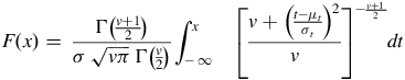
The Generalised t distribution’s mean, median, mode and variance are given by

(7) $$mean = {\mu _t},\;\;\;v \gt 1$$

(8) $$variance = {\sigma _t}{v \over {v - 2}},\;v \gt 2$$

(9) $$mode = median = \;{\mu _t}$$

The GEV distribution (Jenkinson, 1955) is a function of three parameters: location (μ), scale (σ) and extreme value index or shape ( $\xi )$ . GEV combines three types of extreme value theory distributions: Gumbel, Fréchet and Weibull $ - $ also known as type (I), type (II) and type (III), respectively. For $\xi = 0$ , the distribution is of the type (I); $\xi $ > 0 is of type (II) and $\xi $ < 0 is of type (III). The GEV distribution has a finite left boundary and has a positive skewness for ξ > 0, a finite right boundary and a positive skewness for ξ < 0, and extends to infinity in both directions for ξ = 0. GEV PDF( $f\left( x \right))$ and CDF( $F\left( x \right))$ are expressed as

(10) $$f\left( x \right) = {1 \over \sigma }\;Q{\left( x \right)^{\xi + 1}}\;{e^{ - Q\left( x \right)}}$$

(11) $$F\left( x \right) = {e^{ - Q\left( x \right)}}$$

(12) $$Q\left( x \right) = \left\{ {\matrix{ {{{\left( {1 + \xi \left( {{{x - \mu } \over \sigma }} \right)} \right)}^{ - 1/\xi }}} & {\xi \ne 0} \cr {} \cr \hskip-14pt{\displaystyle{e^{\displaystyle\left( { - {{x - \mu } \over \sigma }} \right)}}} & {\xi = 0} \cr } } \right\}$$

The GEV distribution’s mean, median, mode and variance are expressed as

(13) $$mean = \left\{ {\matrix{ {\mu + \sigma {{{\rm{\Gamma }}\left( {1 - \xi } \right) - 1\;} \over \xi }} & {\xi \ne 0,\;\xi \lt 1} \cr {\mu + \sigma \gamma } & {\xi = 0} \cr \infty & {\xi \ge 1} \cr } } \right\}$$

(14) $$\gamma = \;\mathop {\lim }\limits_{n \to \infty } \left( {\mathop \sum \limits_{i = 1\;}^{n\;} {1 \over k} - logn\;} \right)$$

(15) $$Variance = \;\left\{ {\matrix{ {{\sigma ^2}\;{{{g_2} - g_1^2} \over {{\xi ^2}}}} & {\xi \ne 0,\;\xi \lt {1 \over 2}} \cr {} \cr {{{\sigma {\pi ^2}} \over 6}} & {\xi = 0} \cr {} \cr \infty & {\xi \ge {1 \over 2}} \cr } } \right\}$$

(16) $${g_k} = {\rm{\Gamma }}\left( {1 - k\xi } \right)$$

(17) $$median = \left\{ {\matrix{ {m + \sigma {{{{\left( {In\;2} \right)}^{ - \xi }} - 1\;\;\;} \over \xi }} & {\xi \ne 0} \cr {\mu - \sigma \;In\left( {In\left( 2 \right)} \right)} & {\xi = 0} \cr } } \right\}$$

2.2. Maximum likelihood

Maximum likelihood estimates PDF parameters $\left( \theta \right)$ by maximising the likelihood function, and is given by

(18) $${L_n}\left( {\theta {\rm{|}}{x_1} \ldots, {x_n}} \right) = {\rm{\;}}\mathop \prod \limits_{i = 1}^n f\left( {\theta {\rm{|}}{x_i}} \right)$$

where $\left( {{x_1}, \ldots .,{x_n}} \right)$ is the data sample, $f(x|\theta )$ the probability density function with $\left( \theta \right)$ parameters and $n$ the sample size.

Maximum likelihood estimation is based on maximising the log-likelihood function, formed to simplify the original function. The function is given by

(19) $$l \left( {\theta ;{x_i}} \right) = In\left( {L\left( {\theta, {x_i}} \right)} \right)$$

The partial derivative with respect to $\theta $ can be set to zero to estimate the parameter, since the goal is to maximise the log-likelihood function.

(20) $${{\partial l } \over {\partial {\theta _i}}} = 0$$

Then, an iterative numerical procedure (e.g. Newton–Raphson) can be employed to solve the equations returned from the partial derivative of the log-likelihood function.

2.3. The Kolmogorov–Smirnov (KS) test

KS tests whether a sample of data came from a population with a specific distribution. This test is based on computing the maximum difference between the empirical CDF (eCDF) and CDF of the hypothesised distribution. The KS test is given by

(21) $$D = {\rm{\;}}\mathop {\max }\limits_n \left( {D_1,{\rm{\;}}{D_2}} \right)$$

(22) $${D_1} = \mathop {\max }\limits_n \left( {F\left( {{x_I}} \right) - {\rm{\;}}eCDF\left( {{x_I}} \right)} \right)$$

(23) $${D_2} = \mathop {\max }\limits_n \left( {eCDF\left( {{x_I}} \right) - {\rm{\;}}F\left( {{x_I}} \right)} \right)$$

The hypothesis that the error sample follows a given error distribution is given by

- Null-Hypothesis ${H_0}$ : the error sample $\left( {{x_1},{\rm{\;}} \ldots, {x_n}} \right)$ follows a hypothesised error distribution

(24) $${\chi ^2} \gt \;\chi _{1 - \alpha, k - s\;}^2$$

- Alternate Hypothesis ${H_1}$ : the error sample $\left( {{x_1},{\rm{\;}} \ldots, {x_n}} \right)$ does not follow a hypothesised error distribution

(25) $${\chi ^2} \ge {\rm{\;}}\chi _{1 - \alpha, k - c{\rm{\;}}}^2$$

The KS test values are employed in this paper to evaluate the overall fitting performance of the candidate distributions.

3. The derived GEV-based Gaussian distribution

GEV-based Gaussian is a Gaussian distribution generated from the GEV distribution (Figure 1). The first step in creating this distribution is to estimate the GEV distribution parameters (mean, scale parameter, shape parameter) using the maximum likelihood estimation. The GEV distribution’s mean and variance are then computed from the GEV distribution’s estimated parameters.

Figure 1. Derivation of GEV-based Gaussian distribution.

The mathematical derivation of the GEV-based Gaussian distribution starts from the likelihood function for the GEV distribution, which is represented by

(26) $$f{\rm{(}}{x_1},{\rm{\;}} \ldots, {\rm{\;}}{x_n}{\rm{|}}{\mu _{GEV}},{\sigma _{GEV}},\xi ) = \mathop \prod \limits_{i = 1}^n f({x_i}|{\mu _{GEV}},{\sigma _{GEV}},\xi )$$

where ${m_{GEV}},{\sigma _{GEV}},\xi $ are the GEV distribution parameters.

Then, the log-likelihood function of the GEV distribution is represented by

(27) $$l \left( {{\mu _{GEV}},{\sigma _{GEV}},\xi ;{x_i}} \right) = In\left( {L\left( {{\mu _{GEV}},{\sigma _{GEV}},\xi |{x_i}} \right)} \right)$$

(28) $$l \left( {{\mu _{GEV}},{\sigma _{GEV}},\xi ;{x_i}} \right) = - n\;In\left( {{\sigma _{GEV}}} \right) + \mathop \sum \limits_{i = 1}^n \left[ {\left( {{1 \over \xi } - 1} \right)In\left( {{y_i}} \right) - {{\left( {{y_i}} \right)}^{{1 \over \xi }}}} \right]$$

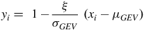(29) $${y_i} = \;1 - {\xi \over {{\sigma _{GEV}}}}\;\left( {{x_i} - {\mu _{GEV}}} \right)$$

To maximise the likelihood function $l \left( {{\mu _{GEV}},{\sigma _{GEV}},\xi ;{x_i}} \right)$ , let the partial derivative of the function with respect to the parameters equal zero.

The partial derivative of the function with respect to the mean is represented, step by step, by

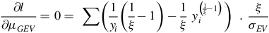(30) $${{\partial l } \over {\partial {\mu _{GEV}}}} = 0 = \;\sum \left( {{1 \over {{y_i}}}\left( {{1 \over \xi } - 1} \right) - {1 \over \xi }\;y_i^{\left( {{1 \over \xi } - 1} \right)}} \right)\;\;.\;{\xi \over {{\sigma _{EV}}}}\;$$

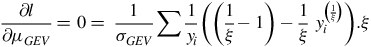(31) $${{\partial l } \over {\partial {\mu _{GEV}}}} = 0 = \;{1 \over {{\sigma _{GEV}}}}\sum {1 \over {{y_i}}}\left( {\left( {{1 \over \xi } - 1} \right) - {1 \over \xi }\;y_i^{\left( {{1 \over \xi }} \right)}} \right).\xi \;$$

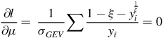(32) $${{\partial l } \over {\partial \mu }} = \;{1 \over {{\sigma _{GEV}}}}\sum {{1 - \xi - y_i^{{1 \over \xi }}} \over {{y_i}}} = 0$$

The partial derivative of the function with respect to the shape parameter is represented by

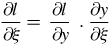(33) $${{\partial l } \over {\partial \xi }} = \;{{\partial l } \over {\partial y}}\;.\;{{\partial y} \over {\partial \xi }}$$

(34) $${{\partial l } \over {\partial \xi }} = {- 1 \over {{\xi ^2}}}\sum \left( {{1 \over 1}In\left( {{y_i}} \right)\left( {1 - \xi - y_i^{{1 \over \xi }}} \right)\;} \right) + {{1 - \xi - y_i^{{1 \over \xi }}} \over {{y_i}}}\;\xi \;\left( {{{{x_i} - {\mu _{GEV}}} \over {{\sigma _{GEV}}}}} \right) = 0$$

To simplify the partial derivative of the function with respect to the sigma, the likelihood function $l \left( {{\mu _{GEV}},{\sigma _{GEV}},\xi ;{x_i}} \right)$ is rewritten as

(35) $$l \left( {{\mu _{GEV}},{\sigma _{GEV}},\xi ;{x_i}} \right) = {\rm{\;}}{l _1}\left( {n,{\sigma _{GEV}}} \right) + {l _2}\left( {{y_i},\xi } \right)$$

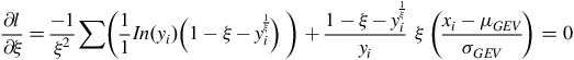
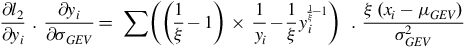
From Equation (36), the partial derivative of the likelihood function with respect to the sigma is derived step by step as follows:

(36) $${{\partial l } \over {\partial {\sigma _{GEV}}}} = {{\partial {l _1}} \over {\partial {\sigma _{GEV}}}} + \;{{\partial {l _2}} \over {\partial {y_i}}}\;.\;{{\partial {y_i}} \over {\partial {\sigma _{GEV}}}}$$

(37) $${{\partial {l _1}} \over {\partial {\sigma _{GEV}}}} = \; {- n \over {{\sigma _{GEV}}}}$$

(38) $${{\partial {l _2}} \over {\partial {y_i}}}\;.\;{{\partial {y_i}} \over {\partial {\sigma _{GEV}}}} = \;\sum \left( {\left( {{1 \over \xi } - 1} \right) \times {1 \over {{y_i}}} - {1 \over \xi }y_i^{{1 \over \xi } - 1}} \right)\;\;.\;{{\xi \;\left( {{x_i} - {\mu _{GEV}}} \right)} \over {\sigma _{GEV}^2}}$$

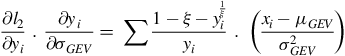(39) $${{\partial {l _2}} \over {\partial {y_i}}}\;.\;{{\partial {y_i}} \over {\partial {\sigma _{GEV}}}} = \;\sum {{1 - \xi - y_i^{{1 \over \xi }}} \over {{y_i}}}\;.\;\;\left( {{{{x_i} - {\mu _{GEV}}} \over {\sigma _{GEV}^2}}} \right)$$

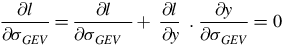(40) $${{\partial l } \over {\partial {\sigma _{GEV}}}} = {{\partial l } \over {\partial {\sigma _{GEV}}\;\;}} + \;{{\partial l } \over {\partial y}}\;.\;{{\partial y} \over {\partial {\sigma _{GEV}}}} = 0$$

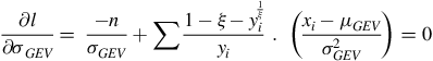(41) $${{\partial l } \over {\partial {\sigma _{GEV}}}} = \; {- n \over {{\sigma _{GEV}}}} + \sum {{1 - \xi - y_i^{{1 \over \xi }}} \over {{y_i}}}\;.\;\;\left( {{{{x_i} - {\mu _{GEV}}} \over {\sigma _{GEV}^2}}} \right) = 0$$

From Equations (32), (35) and (41), the three GEV parameters are estimated using the Newton–Raphson method. Then, the GEV distribution variance is computed using the estimated parameters, represented by

(42) $${\rm{Variance}} = \left\{ {\matrix{ {{{{\sigma _{GEV}}\left( {{g_2} - g_1^2} \right)} \over {{\xi ^2}}}} & {\xi \ne 0\;,\;\xi \lt {1 \over 2}} \cr {\sigma _{GEV}^2 \times {{{\pi ^2}} \over 6}} & {\xi = 0} \cr \infty & {\xi \ge {1 \over 2}} \cr } } \right\}$$

(43) $${g_k}\; = \;\Gamma \left( {1 - k\xi } \right)$$

Then, the GEV-based Gaussian distribution parameters $\;\left( {{\mu _{GbG,\;\;\;}}\sigma _{GbG\;}} \right)$ are computed by

(44) $${\mu _{GbG\;\;}} = {\mu _{GEV}}$$

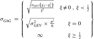(45) $${\sigma _{GbG\;}} = \left\{ {\matrix{ {\sqrt {{{{\sigma _{GEV}}\left( {{g_2} - g_1^2} \right)} \over {{\xi ^2}}}} } & {\xi \ne 0\;,\;\xi \lt {1 \over 2}} \cr {\sqrt {\sigma _{GEV}^2 \times {{{\pi ^2}} \over 6}} } & {\xi = 0} \cr \infty & {\xi \ge {1 \over 2}} \cr } } \right\}$$

4. Results

This section provides a summary of the results from Graphical and KS assessments. The GEV-based Gaussian distribution is tested against the Gaussian, GEV and Generalised t distributions.

In total, 26 datasets were collected over 26 different days in dynamic mode and in mixed environments (urban, semi-urban and open sky). The data were collected using a vehicle-mounted multi-constellation GNSS receiver (Ublox’s F9 receiver) and Trimble’s Applanix reference system. Data collection was carried out in Switzerland, spanning a route of approximately 3,455 km through various cities and regions, as illustrated in the map presented in Figure 2. The data encompass a variety of environments: highways represent open-sky conditions, sometimes bordering on semi-urban areas, while cities like Zürich and Thalwil exemplify urban environments. The vehicle maintained an average speed of approximately 70 km/h, with a minimum of 42 km/h and a maximum of 142 km/h.

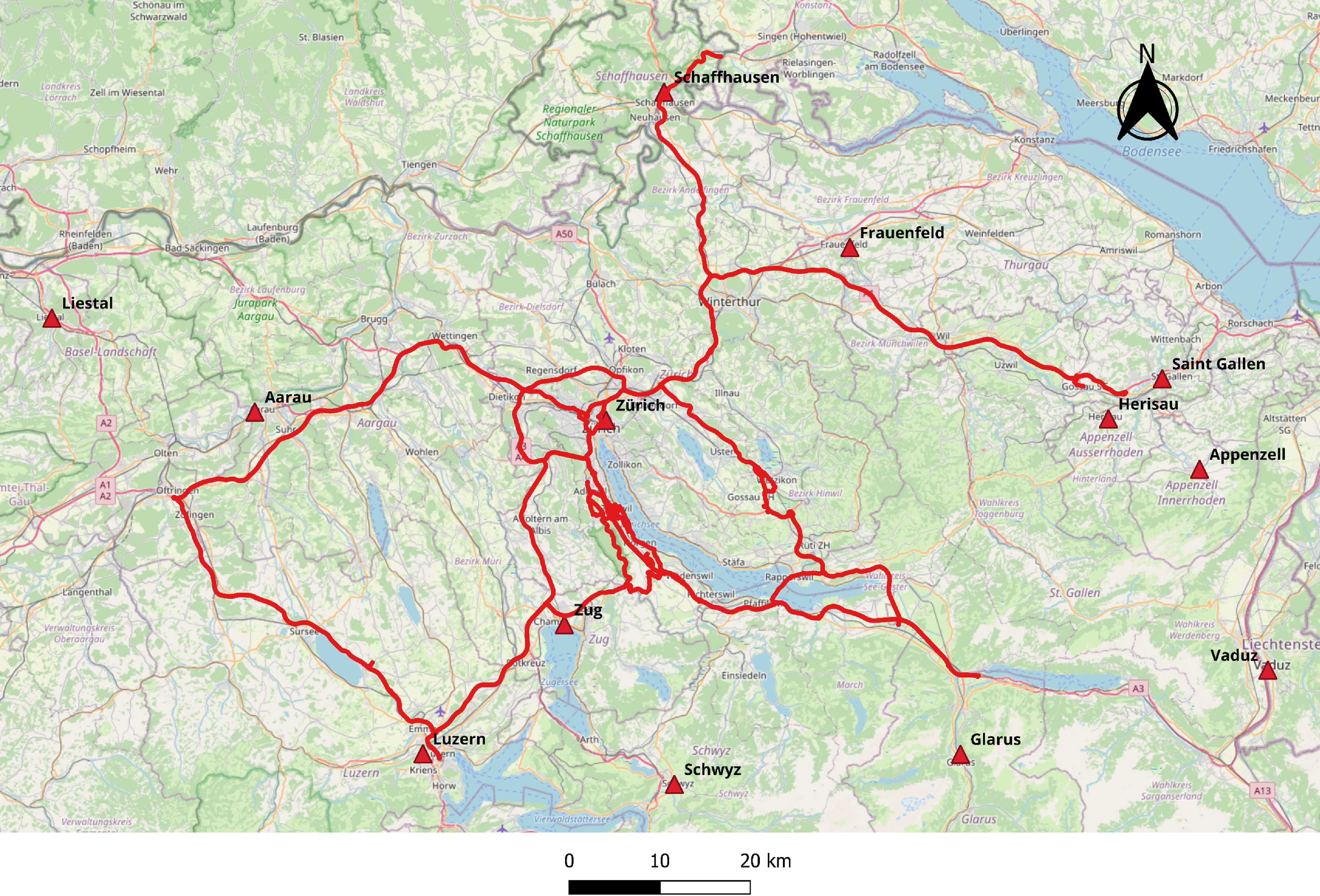
Figure 2. Map of the data collection route (∼3,455 km) used in this study.

The position, velocity, heading and accuracy data were generated using an Applanix reference system and Applanix post-processing software, with an average among all datasets with horizontal accuracy of 4 cm and vertical accuracy of 6 cm. Given the high level of accuracy from the reference system, the range computed from this system was considered the true value. Subsequently, measurement errors were estimated by comparing data from the GNSS receiver with the reference system resulting in more than 2 million rows of pseudorange and carrier phase errors. The GNSS receiver employed divergence-free carrier smoothing techniques, and the truth system’s results were used as a baseline to estimate the residuals.

4.1. Kolmogorov–Smirnov test assessment

KS assessment tests the GEV-based Gaussian distribution for overall fitting, which reflect the positioning reliability. Since the test is based on the maximum difference between CDF and ECDF, it gives an indication of the overall fitting, which might not be sufficient to evaluate the goodness-of-fit in some cases.

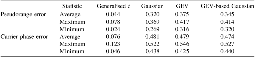
By comparing the KS test values, the results show that the Generalised t distribution is the best of the three candidate distributions in terms of fitting pseudorange and carrier phase error, as seen in all datasets, as shown in Table 1.

Table 1. Average, minimum and maximum KS test values for the 26 datasets.

Mixed results are seen when the remaining three distributions are compared: Gaussian, GEV and GEV-based Gaussian distribution. Table 2 shows the number of times that the value of the test is the lowest between the three distributions for carrier phase and pseudorange error datasets.

Table 2. Number of datasets so that the value of the test is the lowest between three distributions for carrier phase and pseudorange error datasets.

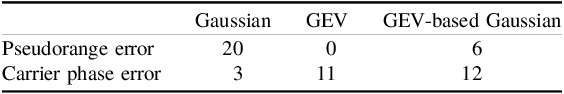
In more detail, for carrier phase error, the KS test values show that the GEV-based Gaussian distribution was the best in terms of fitting between the three distributions in 12 datasets, followed by the GEV distribution, which was the best in 11 datasets, while Gaussian was best in three datasets. For pseudorange error, the results show that the Gaussian distribution is the best with 20 datasets, followed by the GEV-based Gaussian distribution with 6 datasets.

Overall, as shown in Tables 1 and 2, the results overall show that Generalised t is the best in fitting the error data, as the average value of KS test in Generalised t is the lowest. The table also shows that GEV-based Gaussian shows better performance than Gaussian and GEV in fitting carrier phase error (complex data sets), while the Gaussian distribution provides better fitting than GEV and GEV-based Gaussian in pseudorange datasets.

4.2. Graphical assessment

The graphical assessment in this section evaluates the GEV-based Gaussian distribution against the three distributions in terms of tail fitting and overbounding, both of which are of special importance for mission-critical applications. The results show that none of the distributions overbound the empirical distribution. However, the GEV-based Gaussian and GEV distributions provide a better bounding at the tails than the Gaussian and Generalised t distributions.

In more detail, for carrier phase error, the results show that the GEV-based Gaussian distribution is the best in terms of overall overbounding, as seen in almost all datasets. This is followed by the GEV distribution, which also shows in many cases slightly better performance in terms of overbounding than the GEV-based Gaussian distribution at the right tails. Figures 3–8 show that the GEV family distribution overbounds more extreme events. This is clearly seen in the CDF left tail, where more extreme events are covered under the distribution tails.

Figure 3. Carrier phase error characterisation, in the PDF domain, for dataset 1.

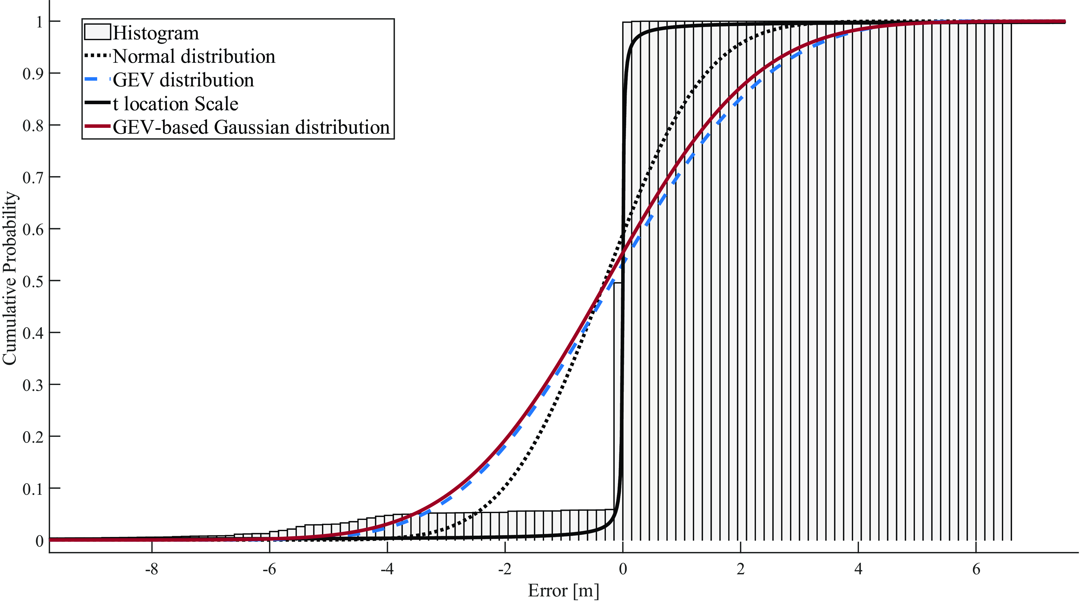
Figure 4. Carrier phase error characterisation, in the CDF domain, for dataset 1.

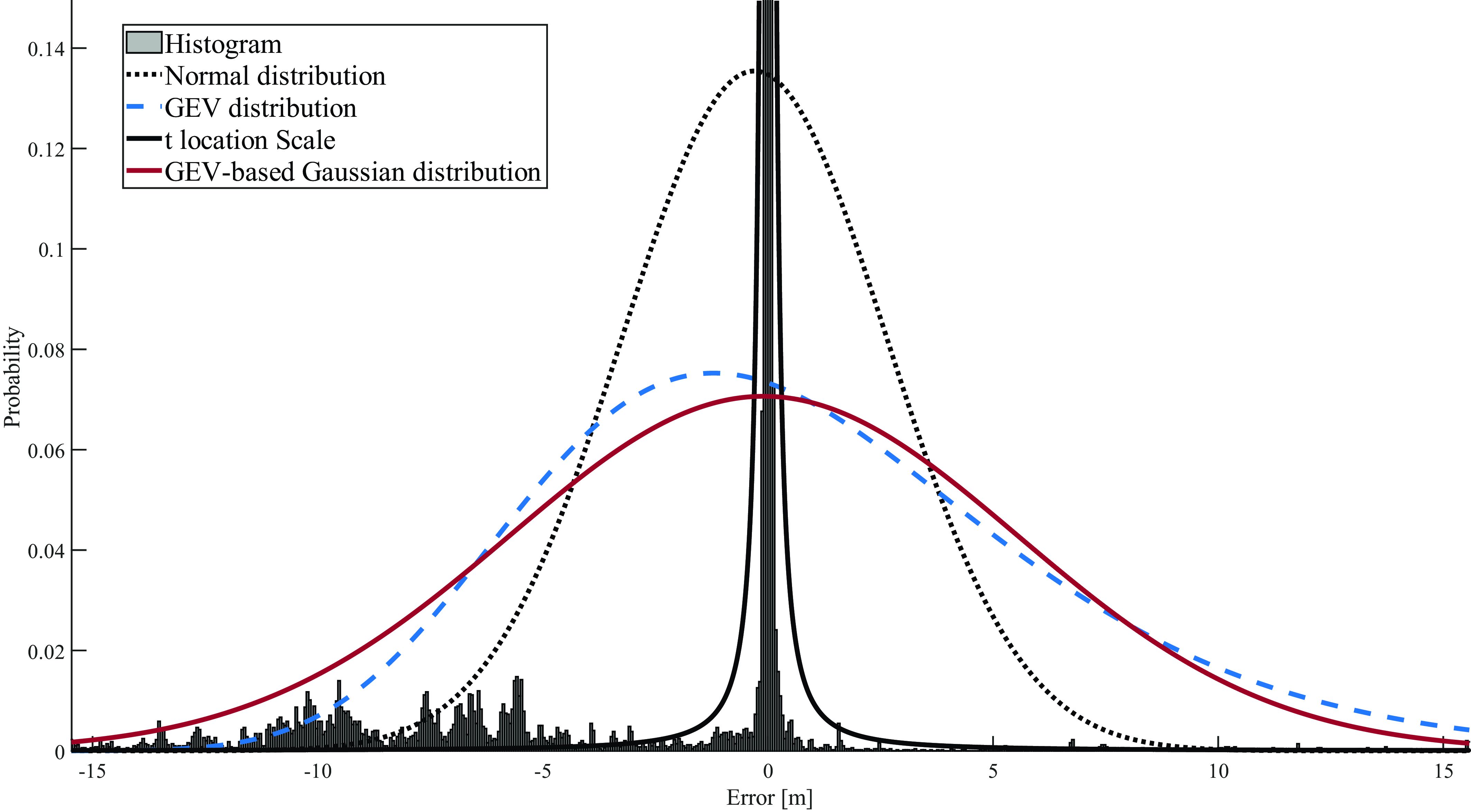
Figure 5. Carrier phase error characterisation, in the PDF domain, for dataset 2.

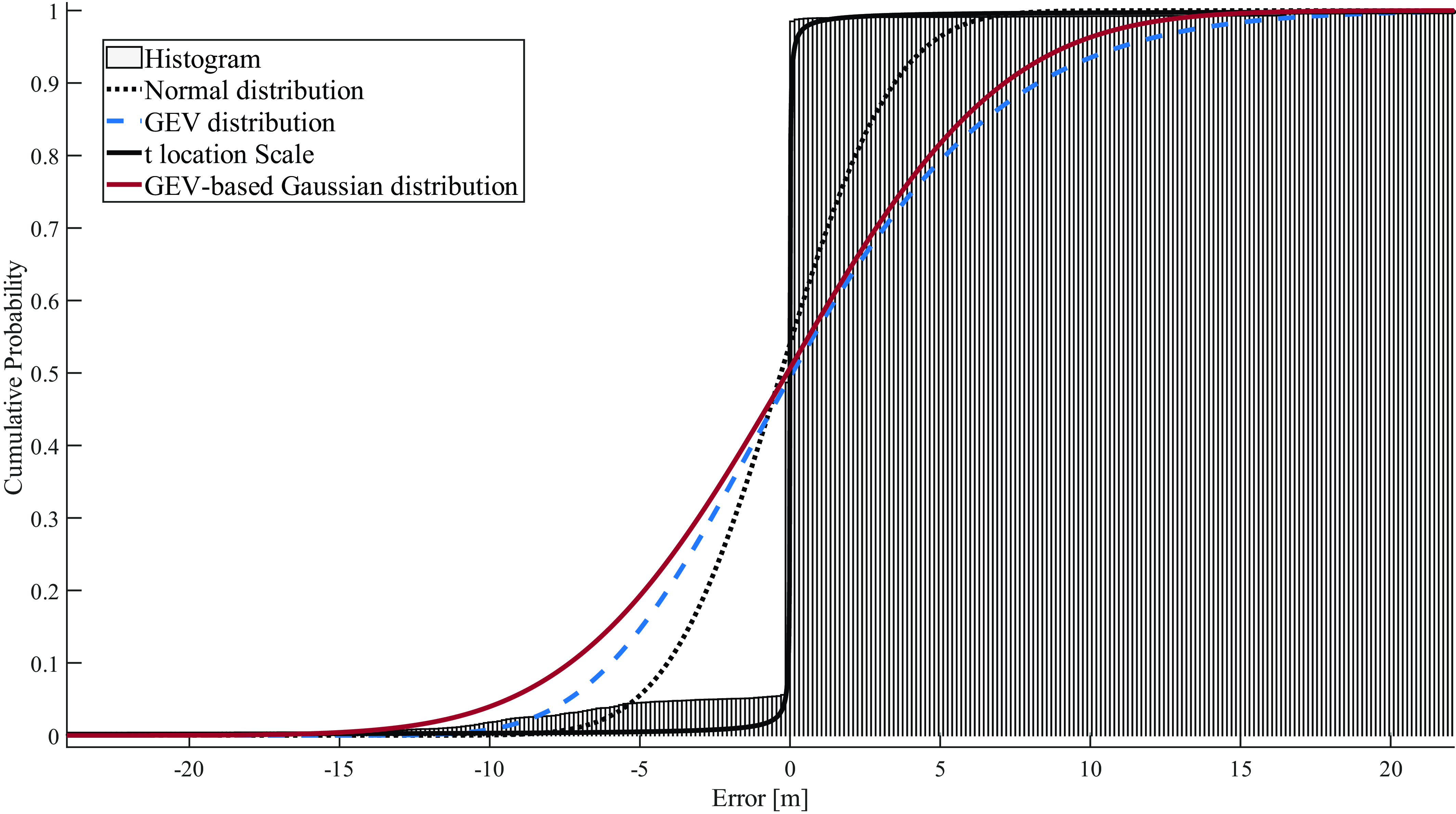
Figure 6. Carrier phase error characterisation, in the CDF domain, for dataset 2.

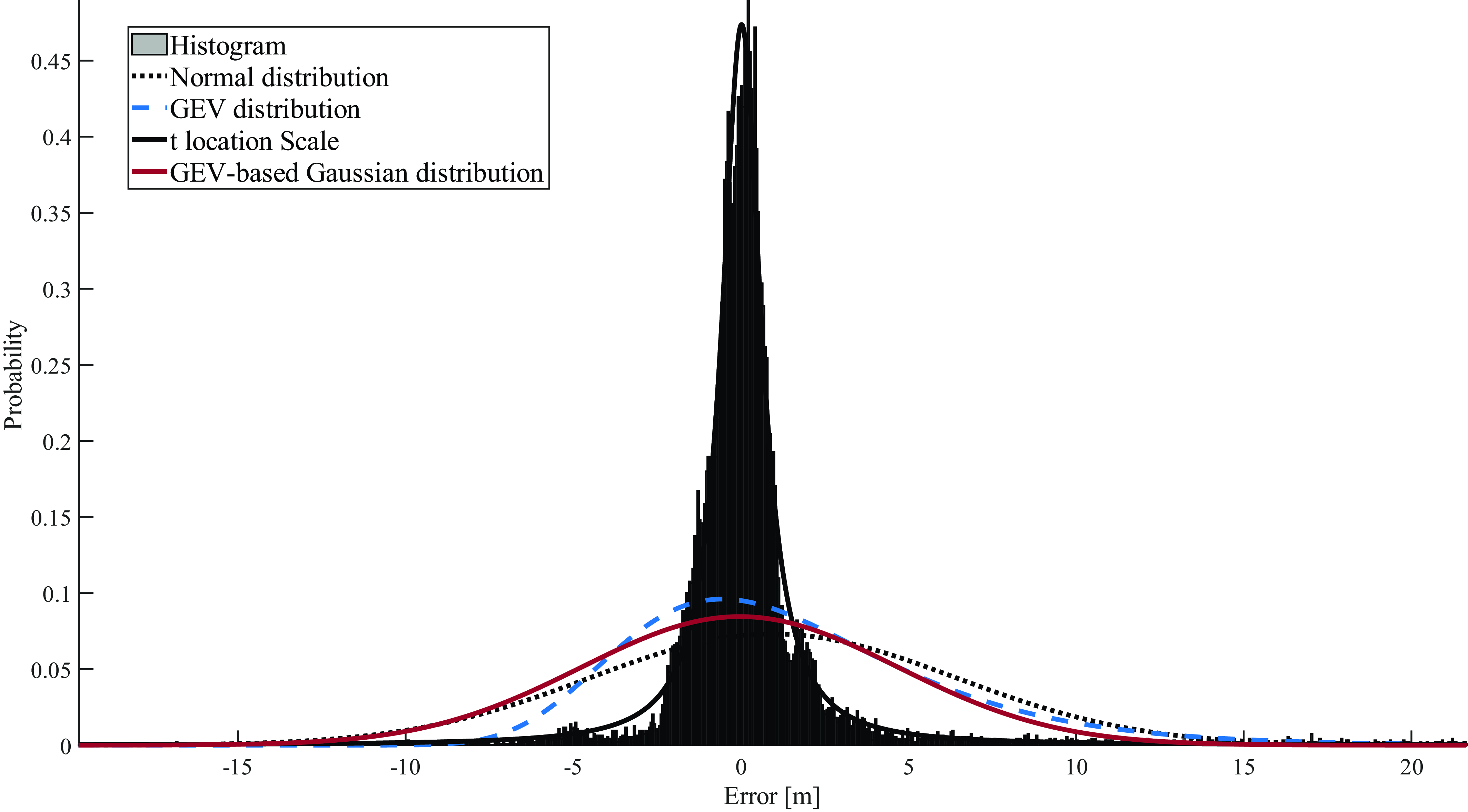
Figure 7. Pseudorange error characterisation, in the PDF domain, for dataset 1.

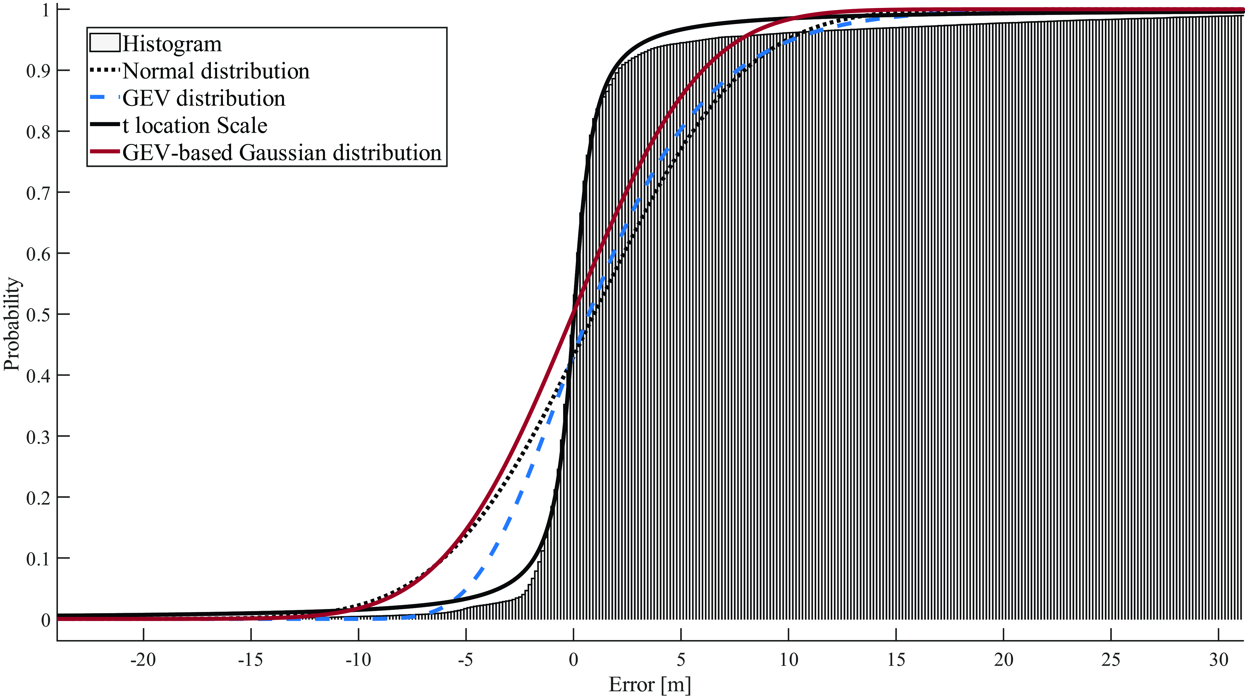
Figure 8. Pseudorange error characterisation, in the CDF domain, for dataset 1.

For pseudorange error, the results show that the GEV and GEV-based Gaussian distributions are the best for bounding. The GEV distribution shows a slightly better performance than the GEV-based Gaussian distribution for overall overbounding, although the latter is best in terms of bounding in the left tail.

In addition, the results also show that the Generalised t distribution provides the best fitting for the majority of the datasets. Mixed results are observed when comparing the remaining three distributions: Gaussian, GEV and GEV-based Gaussian distribution. For tail fitting, the results show that GEV and GEV-based Gaussian distributions are the best of the four distributions.

Overall, the results show that the GEV-based Gaussian distribution is the best among tested distributions in terms of overbounding carrier phase error, followed by the GEV distribution. The corresponding distributions for pseudorange error are GEV and GEV-based Gaussian. Furthermore, both the GEV distribution and the GEV-based Gaussian distribution exhibit superior tail fitting compared with the other two distributions, while Generalised t provides the best fitting for the core.

4.3. Summary

The proposed distribution has been tested against three distributions (Gaussian, GEV and Generalised t) in two aspects: fitting (overall and tail) and overbounding.

The KS and graphical assessment show that Generalised t provides the best overall fitting for the pseudorange and carrier phase error among the four distributions, followed by GEV-based Gaussian for carrier phase error and Gaussian for pseudorange error. Furthermore, the graphical assessments show that the GEV family (GEV and GEV-based Gaussian) provides the best fitting for the tail.

In addition, the graphical assessment shows that the GEV family provides better overall bounding for pseudorange and carrier phase error. Specifically, the GEV-based Gaussian distribution exhibits better overbounding for the carrier phase error, while the GEV distribution shows better overbounding results for the pseudorange error.

5. Conclusions

This paper proposes a derived distribution generated from the GEV and Gaussian distributions, referred to as the GEV-based Gaussian distribution, to take advantage of both distributions. The results have shown that the distribution combines the GEV distribution’s ability in mapping extreme events, with Gaussian distribution simplicity in computation and error propagation.

The GEV-based Gaussian distribution has been tested using Kolmogorov–Smirnov test (KS), and graphical assessment against Gaussian, GEV distribution and Generalised t.

The assessments have shown that none of the tested distributions overbounds the empirical distribution. However, the results show that the novel GEV-based Gaussian distribution is the best in terms of bounding extreme events in the carrier phase error datasets, followed by the GEV distribution. Furthermore, the GEV distribution is the best in terms of bounding the pseudorange error, followed by the GEV-based Gaussian distribution.

Due to the GEV distribution’s complexity compared with the Gaussian distribution in the error convolution process, this paper proposes using GEV-based Gaussian distribution for monitoring GNSS integrity for mission-critical applications, while accounting for the needs for overbounding.

The GEV-based Gaussian distribution can be applied to both system-level and user-level integrity monitoring. At the system level, errors can be characterised using this distribution through integrity monitoring system reference stations and Continuously Operating Reference Station (CORS) networks, with the distribution’s parameters transmitted to users via satellite-based or ground-based augmentation systems. Users can then use this information to enhance positioning and navigation safety compared with conventional Gaussian-based approaches. Research is ongoing to evaluate the impact of using the GEV-based Gaussian distribution in the positioning domain.