

1. Introduction
Modern macroeconomic models often utilize a representative household or assume a fixed composition of heterogeneous households. However, when households with differing characteristics also have varying fertility rates, the composition of the population evolves over time. This process, referred to as natural selection, can have profound implications for the macroeconomy. This study investigates how household heterogeneity and natural selection influence economic growth, particularly through their effects on education, human capital accumulation and innovation.
Households differ in their attitudes toward education and their ability to transmit human capital across generations. These differences persist over time and shape economic outcomes. For instance, Alesina et al. (Reference Alesina, Seror, Yang, You and Zeng2021) show that family attitudes toward education can remain stable even after significant policy interventions. Unfortunately, not all households are equally endowed with the ability to accumulate human capital, leading to disparities in education and fertility choices. This raises important questions: how does household heterogeneity affect fertility decisions? And how do these decisions, in turn, impact technological progress and growth?
To address these questions, we develop an innovation-driven growth model that incorporates fertility choices, natural selection among heterogeneous households and endogenous activation of innovation. Our model extends the unified growth theory pioneered by Galor (Reference Galor2005, Reference Galor2011, Reference Galor2022), which posits that households differ in their ability to accumulate human capital. In our framework, families with greater educational abilities prioritize child quality over quantity, resulting in fewer children but higher levels of human capital. Using panel data from 137 countries, we illustrate this well-documented negative relationship between fertility and education in Figure 1. This quality-quantity tradeoff, also supported by empirical evidence from studies such as Becker et al. (Reference Becker, Cinnirella and Woessmann2010), Fernihough (Reference Fernihough2017) and Klemp and Weisdorf (Reference Klemp and Weisdorf2019), implies an evolutionary advantage to families who choose to have more children but less education. We use our growth-theoretic framework to explore how this evolutionary process affects human capital accumulation, innovation and economic growth.
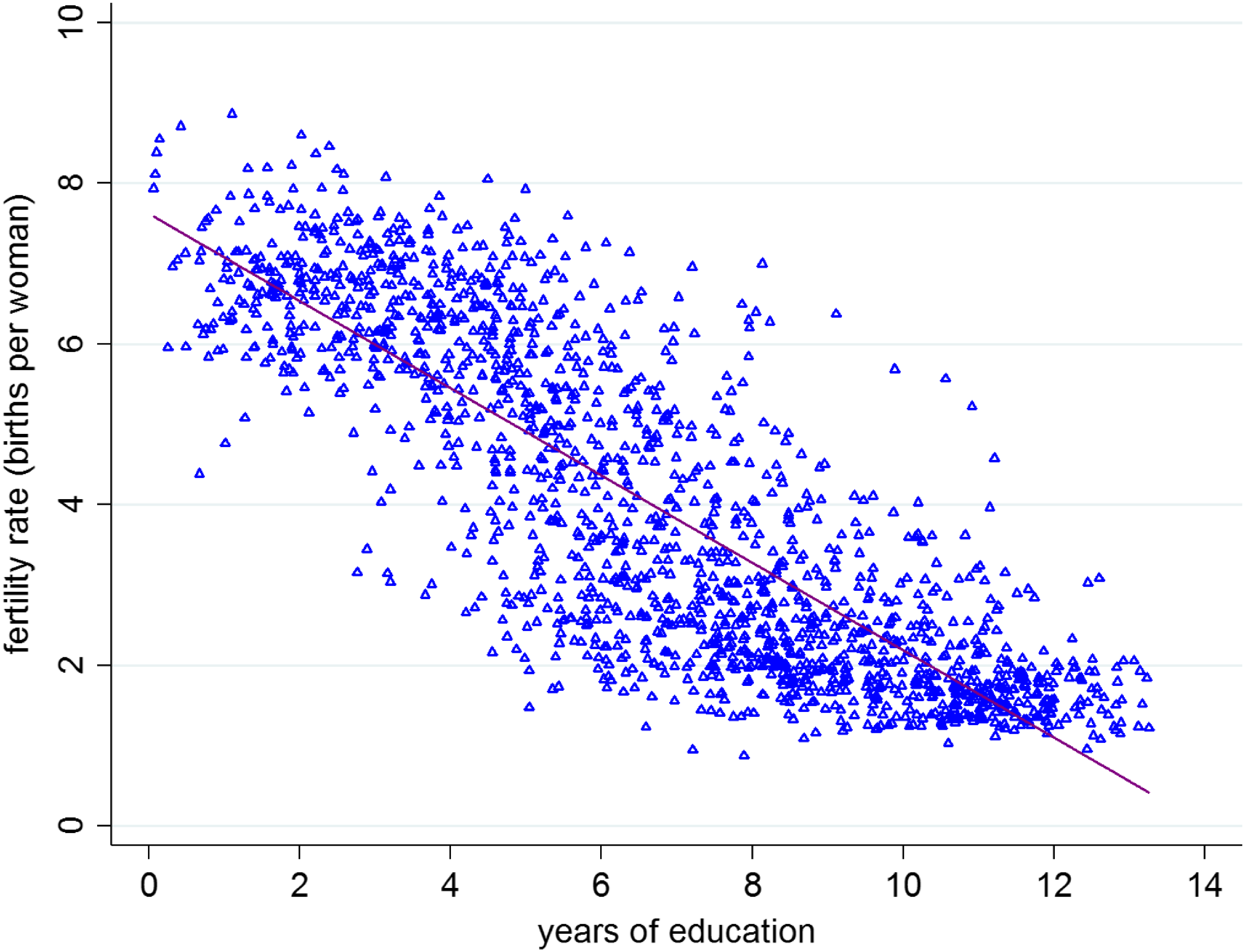
Figure 1. Fertility and education.Notes: This figure depicts the negative correlation between fertility and education. The vertical axis represents the fertility rate, whereas the horizontal axis denotes the number of years of education.
In our model, the evolutionary disadvantage of households with higher educational abilities are temporary. As the economy progresses, they eventually accumulate more human capital, leading to a convergence in fertility rates across households and a stationary distribution of population shares. One of the key insights of our model is that household heterogeneity can initially enhance the likelihood of innovation by increasing the total amount of human capital available for production and research and development (R&D) activities. However, this advantage is offset by the evolutionary disadvantage faced by high-ability households during transitional dynamics, which leads to a decline in their population share and, consequently, a reduction in the overall level of human capital in the economy. This evolutionary process results in a population that is, on average, less educated than it would be in the absence of natural selection, with significant implications for long-term economic growth. This finding resonates with the following observation: “Britons are becoming less educated and poorer because smart rich people are having fewer children.”Footnote 1 A contribution of this study is to show that this phenomenon may be universal and not be specific to Britain.
Our findings also suggest that the temporary evolutionary advantage enjoyed by lower-ability households due to higher fertility rates has permanent effects on the economy’s growth trajectory. Specifically, the scale-invariant nature of our model implies that the economy’s steady-state growth rate is lower when the share of high-ability households decreases over time. We provide empirical evidence supporting this theory, demonstrating that heterogeneity in educational abilities adversely affects education, innovation, and economic growth in the long run. These results hold even when ancestral population diversity and prehistoric migratory distances in Ashraf and Galor (Reference Ashraf and Galor2013) are used as instrumental variables for educational heterogeneity.
Furthermore, this study not only advances the theoretical understanding of the dynamics between natural selection, household heterogeneity and economic growth but also provides actionable insights for addressing real-world challenges. Specifically, our findings suggest that interventions aimed at reducing educational disparities—such as meritocratic reforms and targeted public investments—can mitigate the evolutionary disadvantage faced by high-ability households and foster sustained innovation and growth.
This study contributes to the literature on innovation and economic growth by examining the complex interplay between natural selection, household heterogeneity, and R&D activities. The pioneering studies in this literature are Romer (Reference Romer1990), Aghion and Howitt (Reference Aghion and Howitt1992), Grossman and Helpman (Reference Grossman and Helpman1991) and Segerstrom et al. (Reference Segerstrom, Anant and Dinopoulos1990) . We follow subsequent studies, such as Jones (Reference Jones2001), Connolly and Peretto (Reference Connolly and Peretto2003), Chu et al. (Reference Chu, Cozzi and Liao2013), Peretto and Valente (Reference Peretto and Valente2015) and Brunnschweiler et al. (Reference Brunnschweiler, Peretto and Valente2021), by introducing endogenous fertility to the innovation-driven growth model in order to explore how endogenous fertility decisions among heterogeneous households shape economic development. A novelty of our analysis is that we allow for heterogeneous households, which give rise to an evolutionary process. We find that the temporary disadvantage faced by high-ability households during transitional periods has lasting consequences for technological progress and long-term growth. Our model provides new insights into these dynamics, offering valuable implications for both economic policy and the theoretical understanding of growth mechanisms.
Our work also relates to the broader literature on endogenous growth and economic transitions. An early study by Galor and Weil (Reference Galor and Weil2000) develops the unified growth theory that explores the endogenous transition of an economy from pre-industrial stagnation to modern economic growth; see Galor (Reference Galor2005, Reference Galor2011, Reference Galor2022) for a comprehensive review of unified growth theory and also Galor and Moav (Reference Galor and Moav2001, Reference Galor and Moav2002), Galor and Mountford (Reference Galor and Mountford2008), Galor, et al. (Reference Galor, Moav and Vollrath2009), Ashraf and Galor (Reference Ashraf and Galor2011), Galor and Michalopoulos (Reference Galor and Michalopoulos2012) and Carillo et al. (Reference Carillo, Lombardo and Zazzaro2019) for subsequent studies and empirical evidence that supports unified growth theory. For example, Galor and Moav (Reference Galor and Moav2002), Galor and Michalopoulos (Reference Galor and Michalopoulos2012) and Carillo et al. (Reference Carillo, Lombardo and Zazzaro2019) explore how natural selection of different traits, such as the quality preference of fertility, the degree of risk aversion and the level of family-specific human capital, affects the transition from stagnation to growth. This study complements these interesting studies by examining how natural selection of heterogeneous households with different ability to accumulate human capital affects the transition of an economy from human capital accumulation to modern economic growth that is driven by R&D and innovation.
Therefore, we also contribute to the related branch of the literature on the endogenous transition from pre-industrial stagnation to modern innovation-driven economic growth. For example, Funke and Strulik (Reference Funke and Strulik2000) and Peretto (Reference Peretto2015) explore how economies transition through different stages of development, including capital accumulation and innovation.Footnote 2 Our study adds to this literature by introducing natural selection to a tractable innovation-driven growth model, highlighting the role of household heterogeneity in shaping these transitions.
The rest of this paper is organized as follows. Section 2 presents the model. Section 3 discusses the two stages of economic development. Section 4 examines the implications of household heterogeneity and natural selection. Section 5 provides empirical evidence supporting our theoretical findings. Finally, Section 6 concludes.
2. An R&D-based growth model with natural selection
To model natural selection, we introduce heterogeneous households and endogenous fertility to the seminal Romer model. To keep the model tractable, we consider a simple structure of overlapping generations (OLG) and human capital accumulation.Footnote 3 Each individual lives for three periods. In the young age, the individual accumulates human capital. In the working age, the individual allocates her time between work, fertility and education of the next generation. In the old age, the individual consumes her saving. Saving is required in the OLG model of innovation-driven growth because inventions are owned by agents as assets.
2.1 Heterogeneous households
There is a unit continuum of households indexed by $i\in \lbrack 0,1]$
. Within household
$i\in \lbrack 0,1]$
. Within household $i$
, the utility of an individual who works at time
$i$
, the utility of an individual who works at time $t$
is given byFootnote
4
$t$
is given byFootnote
4
 \begin{equation} U^{t}(i)=u\left [ n_{t}(i),h_{t+1}(i),c_{t+1}(i)\right ] =\eta \ln n_{t}(i)+\gamma \ln h_{t+1}(i)+\ln c_{t+1}(i)\text {,} \end{equation}
where $c_{t+1}(i)$
is the individual’s consumption at time
$c_{t+1}(i)$
is the individual’s consumption at time $t+1$
,
$t+1$
, $n_{t}(i)$
denotes the number of children the individual has at time
$n_{t}(i)$
denotes the number of children the individual has at time $t$
,
$t$
, $\eta \gt 0$
is the fertility preference parameter,
$\eta \gt 0$
is the fertility preference parameter, $h_{t+1}(i)$
denotes the level of human capital that the individual passes onto each child, and
$h_{t+1}(i)$
denotes the level of human capital that the individual passes onto each child, and $\gamma$
is the quality preference parameter. We assume that all individuals within the same household
$\gamma$
is the quality preference parameter. We assume that all individuals within the same household $i$
have the same level of human capital at time 0. Then, they will also have the same level of human capital for all
$i$
have the same level of human capital at time 0. Then, they will also have the same level of human capital for all $t$
as an endogenous outcome.
$t$
as an endogenous outcome.
The individual allocates $e_{t}(i)$
units of time to her children’s education. The accumulation equation of human capital is given byFootnote
5
$e_{t}(i)$
units of time to her children’s education. The accumulation equation of human capital is given byFootnote
5
 \begin{equation} h_{t+1}(i)=\phi (i)e_{t}(i)+(1-\delta )h_{t}(i)\text {,} \end{equation}
where the parameter $\delta \in (0,1)$
is the depreciation rate of human capital that a generation passes onto the next.Footnote
6
,
Footnote
7
As for the ability parameter
$\delta \in (0,1)$
is the depreciation rate of human capital that a generation passes onto the next.Footnote
6
,
Footnote
7
As for the ability parameter $\phi (i)\gt 0$
of household
$\phi (i)\gt 0$
of household $i$
,Footnote
8
it is heterogeneous across households and follows a general distribution with the following mean:Footnote
9
$i$
,Footnote
8
it is heterogeneous across households and follows a general distribution with the following mean:Footnote
9
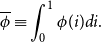 \begin{equation*} \overline {\phi }\equiv \int _{0}^{1}\phi (i)di\text {.} \end{equation*}
The heterogeneity of households is captured by their differences in $\phi (i)$
, which in turn give rise to an endogenous distribution of human capital. We focus on heterogeneity in
$\phi (i)$
, which in turn give rise to an endogenous distribution of human capital. We focus on heterogeneity in $\phi (i)$
because it allows for a stationary distribution of the population share of different households in the long run, whereas heterogeneity in other parameters, such as
$\phi (i)$
because it allows for a stationary distribution of the population share of different households in the long run, whereas heterogeneity in other parameters, such as $\eta$
or
$\eta$
or $\gamma$
, imply that households with the largest
$\gamma$
, imply that households with the largest $\eta$
or smallest
$\eta$
or smallest $\gamma$
would dominate the population in the long run.
$\gamma$
would dominate the population in the long run.
An individual in household $i$
allocates
$i$
allocates $1-e_{t}(i)-\sigma n_{t}(i)$
units of time to work and earns
$1-e_{t}(i)-\sigma n_{t}(i)$
units of time to work and earns $w_{t}\left [ 1-e_{t}(i)-\sigma n_{t}(i)\right ] h_{t}(i)$
as real wage income, where the parameter
$w_{t}\left [ 1-e_{t}(i)-\sigma n_{t}(i)\right ] h_{t}(i)$
as real wage income, where the parameter $\sigma \in (0,1)$
determines the time cost
$\sigma \in (0,1)$
determines the time cost $\sigma n_{t}(i)$
of fertility.Footnote
10
For simplicity, we assume that there are economies of scale in the time spent in educating children within a family, and the cost of having more children is reflected in the time cost of childrearing.Footnote
11
$\sigma n_{t}(i)$
of fertility.Footnote
10
For simplicity, we assume that there are economies of scale in the time spent in educating children within a family, and the cost of having more children is reflected in the time cost of childrearing.Footnote
11
The individual devotes her entire wage income to saving at time $t$
and consumes the return at time
$t$
and consumes the return at time $t+1$
:Footnote
12
$t+1$
:Footnote
12
 \begin{equation} c_{t+1}(i)=(1+r_{t+1})w_{t}\left [ 1-e_{t}(i)-\sigma n_{t}(i)\right ] h_{t}(i)\text {,} \end{equation}
where $r_{t+1}$
is the real interest rate. Substituting (2) and (3) into (1), the individual maximizes
$r_{t+1}$
is the real interest rate. Substituting (2) and (3) into (1), the individual maximizes
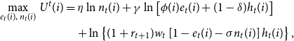 \begin{align*} \underset {e_{t}(i),\text { }n_{t}(i)}{\max }\text { }U^{t}(i)&=\eta \ln n_{t}(i)+\gamma \ln \left [ \phi (i)e_{t}(i)+(1-\delta )h_{t}(i)\right ] \\ \nonumber &\quad+ \ln \left \{ (1+r_{t+1})w_{t}\left [ 1-e_{t}(i)-\sigma n_{t}(i)\right ] h_{t}(i)\right \} \text {,} \end{align*}
taking $\{r_{t+1},w_{t},h_{t}(i)\}$
as given. The utility-maximizing level of fertility
$\{r_{t+1},w_{t},h_{t}(i)\}$
as given. The utility-maximizing level of fertility $n_{t}(i)$
is
$n_{t}(i)$
is
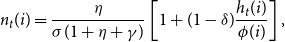 \begin{equation} n_{t}(i)=\frac {\eta }{\sigma (1+\eta +\gamma )}\left [ 1+(1-\delta )\frac {h_{t}(i)}{\phi (i)}\right ] \text {,} \end{equation}
which is decreasing in $\phi (i)$
but increasing in
$\phi (i)$
but increasing in $h_{t}(i)$
. In other words, households with a lower ability to accumulate human capital and a higher level of human capital choose to have more children. In (4), fertility
$h_{t}(i)$
. In other words, households with a lower ability to accumulate human capital and a higher level of human capital choose to have more children. In (4), fertility $n_{t}(i)$
is decreasing in
$n_{t}(i)$
is decreasing in $\phi (i)/h_{t}(i)$
. As we will show, households with higher
$\phi (i)/h_{t}(i)$
. As we will show, households with higher $\phi (i)$
have higher
$\phi (i)$
have higher $h_{t}(i)$
and also higher
$h_{t}(i)$
and also higher $\phi (i)/h_{t}(i)$
before the level of human capital reaches the steady state, at which point all households share the same
$\phi (i)/h_{t}(i)$
before the level of human capital reaches the steady state, at which point all households share the same $\phi (i)/h_{t}(i)$
. Therefore, households with higher ability
$\phi (i)/h_{t}(i)$
. Therefore, households with higher ability $\phi (i)$
generally have higher human capital
$\phi (i)$
generally have higher human capital $h_{t}(i)$
and lower fertility
$h_{t}(i)$
and lower fertility $n_{t}(i)$
, generating a negative relationship between these two variables. To understand this negative relationship, we also derive the utility-maximizing level of education
$n_{t}(i)$
, generating a negative relationship between these two variables. To understand this negative relationship, we also derive the utility-maximizing level of education $e_{t}(i)$
asFootnote
13
$e_{t}(i)$
asFootnote
13
 \begin{equation} e_{t}(i)=\frac {1}{1+\eta +\gamma }\left [ \gamma -(1+\eta )(1-\delta )\frac {h_{t}(i)}{\phi (i)}\right ] \text {,} \end{equation}
which is increasing in $\phi (i)$
but decreasing in
$\phi (i)$
but decreasing in $h_{t}(i)$
. In summary, for a given
$h_{t}(i)$
. In summary, for a given $h_{t}(i)$
, households with a larger
$h_{t}(i)$
, households with a larger $\phi (i)$
choose a higher level of education
$\phi (i)$
choose a higher level of education $e_{t}(i)$
but a smaller number
$e_{t}(i)$
but a smaller number $n_{t}(i)$
of children, reflecting the quality-quantity tradeoff. Given the same initial human capital
$n_{t}(i)$
of children, reflecting the quality-quantity tradeoff. Given the same initial human capital $h_{0}(i)=h_{0}$
, differences in education ability
$h_{0}(i)=h_{0}$
, differences in education ability $\phi (i)$
give rise to differences in education level
$\phi (i)$
give rise to differences in education level $e_{t}(i)$
.Footnote
14
$e_{t}(i)$
.Footnote
14
Substituting (5) into (2) yields the autonomous and stable dynamics of human capital as
 \begin{equation} h_{t+1}(i)=\frac {\gamma }{1+\eta +\gamma }\left [ \phi (i)+(1-\delta )h_{t}(i)\right ] \text {,} \end{equation}
where $h_{t+1}(i)$
is increasing in
$h_{t+1}(i)$
is increasing in $\phi (i)$
and
$\phi (i)$
and $h_{t}(i)$
. The total amount of human capital in the economy at time
$h_{t}(i)$
. The total amount of human capital in the economy at time $t$
is
$t$
is
 \begin{equation*} H_{t}=\int _{0}^{1}h_{t}(i)L_{t}(i)di\text {,} \end{equation*}
where $L_{t}(i)$
is the working-age population size of household
$L_{t}(i)$
is the working-age population size of household $i$
. The law of motion for
$i$
. The law of motion for $L_{t}(i)$
is
$L_{t}(i)$
is
 \begin{equation} L_{t+1}(i)=n_{t}(i)L_{t}(i)=\frac {\eta }{\sigma (1+\eta +\gamma )}\left [ 1+(1-\delta )\frac {h_{t}(i)}{\phi (i)}\right ] L_{t}(i)\text {,} \end{equation}
and the size of the aggregate labor force in the economy at time $t$
is
$t$
is
 \begin{equation*} L_{t}=\int _{0}^{1}L_{t}(i)di\text {.} \end{equation*}
Let’s define $s_{t}(i)\equiv L_{t}(i)/L_{t}$
as the working-age-population (i.e., labor) share of household
$s_{t}(i)\equiv L_{t}(i)/L_{t}$
as the working-age-population (i.e., labor) share of household $i$
.
$i$
.
Lemma 1.
The labor share $s_{t}(i)$
of household
$s_{t}(i)$
of household $i$
at time
$i$
at time $t\geq 1$
is given by
$t\geq 1$
is given by
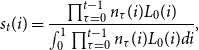 \begin{equation*} s_{t}(i)=\frac {\prod \nolimits _{\tau =0}^{t-1}n_{\tau }(i)L_{0}(i)}{ \int _{0}^{1}\prod \nolimits _{\tau =0}^{t-1}n_{\tau }(i)L_{0}(i)di}\text {,} \end{equation*}
where the fertility decision $n_{t}(i)$
of household
$n_{t}(i)$
of household $i$
at time
$i$
at time $t\geq 1$
is given by
$t\geq 1$
is given by
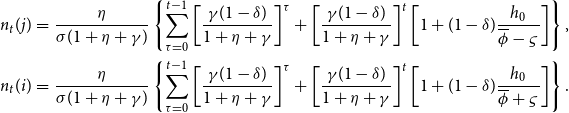
 \begin{equation*} n_{t}(i)=\frac {\eta }{\sigma (1+\eta +\gamma )}\left \{ \sum _{\tau =0}^{t-1}\left [ \frac {\gamma (1-\delta )}{1+\eta +\gamma }\right ] ^{\tau }+\left [ \frac {\gamma (1-\delta )}{1+\eta +\gamma }\right ] ^{t}\left [ 1+(1-\delta )\frac {h_{0}(i)}{\phi (i)}\right ] \right \} \text {,} \end{equation*}
which is a decreasing function of $\phi (i)/h_{0}(i)$
.
$\phi (i)/h_{0}(i)$
.
Proof. See Appendix A.
Notice that changes to $n_{\tau }(i)$
in any one period will affect
$n_{\tau }(i)$
in any one period will affect $s_{t}(i)$
in all future generations. The reason is general and does not depend on the specific assumptions of this model: a temporary growth effect has a permanent level effect. Therefore, if the fertility rate of an ability group drops temporarily, this group would ceteris paribus forever have a lower population share than it would otherwise have had. As we will later see, if the high-ability household experiences a temporary reproduction loss, the economy will have a lower share of high-ability people forever. We will also show that this loss will permanently lower human capital, innovation and growth.
$s_{t}(i)$
in all future generations. The reason is general and does not depend on the specific assumptions of this model: a temporary growth effect has a permanent level effect. Therefore, if the fertility rate of an ability group drops temporarily, this group would ceteris paribus forever have a lower population share than it would otherwise have had. As we will later see, if the high-ability household experiences a temporary reproduction loss, the economy will have a lower share of high-ability people forever. We will also show that this loss will permanently lower human capital, innovation and growth.
2.2 Final good
Perfectly competitive firms use the following production function to produce final good $Y_{t}$
, which is chosen as the numeraire:
$Y_{t}$
, which is chosen as the numeraire:
 \begin{equation} Y_{t}=H_{Y,t}^{1-\alpha }\int _{0}^{N_{t}}X_{t}^{\alpha }(j)dj\text {,} \end{equation}
where the parameter $\alpha \in (0,1)$
determines production labor intensity
$\alpha \in (0,1)$
determines production labor intensity $1-\alpha$
, and
$1-\alpha$
, and $H_{Y,t}$
denotes human-capital-embodied production labor.
$H_{Y,t}$
denotes human-capital-embodied production labor. $X_{t}(j)$
denotes a continuum of differentiated intermediate goods indexed by
$X_{t}(j)$
denotes a continuum of differentiated intermediate goods indexed by $j\in \lbrack 0,N_{t}]$
. Firms maximize profit, and the conditional demand functions for
$j\in \lbrack 0,N_{t}]$
. Firms maximize profit, and the conditional demand functions for $H_{Y,t}$
and
$H_{Y,t}$
and $X_{t}(j)$
are given by
$X_{t}(j)$
are given by
 \begin{equation} w_{t}=(1-\alpha )\frac {Y_{t}}{H_{Y,t}}\text {,} \end{equation}
 \begin{equation} p_{t}(j)=\alpha \left [ \frac {H_{Y,t}}{X_{t}(j)}\right ] ^{1-\alpha }\text {.} \end{equation}
2.3 Intermediate goods
Each intermediate good $j$
is produced by a monopolistic firm, which uses a one-to-one linear production function that transforms
$j$
is produced by a monopolistic firm, which uses a one-to-one linear production function that transforms $X_{t}(j)$
units of final good into
$X_{t}(j)$
units of final good into $X_{t}(j)$
units of intermediate good
$X_{t}(j)$
units of intermediate good $j\in \lbrack 0,N_{t}]$
. The profit function is
$j\in \lbrack 0,N_{t}]$
. The profit function is
 \begin{equation} \pi _{t}(j)=p_{t}(j)X_{t}(j)-X_{t}(j)\text {,} \end{equation}
where the marginal cost of production is constant and equal to one (recall that final good is the numeraire). The monopolist maximizes (11) subject to (10) to derive the monopolistic price as
 \begin{equation} p_{t}(j)=\min \left \{ \mu ,\frac {1}{\alpha }\right \} =\mu \gt 1\text {,} \end{equation}
where $\mu \leq 1/\alpha$
is a patent policy parameter as in Li (Reference Li2001) and Goh and Olivier (Reference Goh and Olivier2002). One can show that
$\mu \leq 1/\alpha$
is a patent policy parameter as in Li (Reference Li2001) and Goh and Olivier (Reference Goh and Olivier2002). One can show that $X_{t}(j)=X_{t}$
for all
$X_{t}(j)=X_{t}$
for all $j\in \lbrack 0,N_{t}]$
by substituting (12) into (10). Then, we substitute (10) and (12) into (11) to derive the equilibrium amount of monopolistic profit as
$j\in \lbrack 0,N_{t}]$
by substituting (12) into (10). Then, we substitute (10) and (12) into (11) to derive the equilibrium amount of monopolistic profit as
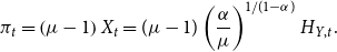 \begin{equation} \pi _{t}=\left ( \mu -1\right ) X_{t}=(\mu -1)\left ( \frac {\alpha }{\mu }\right ) ^{1/(1-\alpha )}H_{Y,t}\text {.} \end{equation}
2.4 R&D
We denote $v_{t}$
as the value of a newly invented intermediate good at the end of time
$v_{t}$
as the value of a newly invented intermediate good at the end of time $t$
. The value of
$t$
. The value of $v_{t}$
is given by the present value of future profits from time
$v_{t}$
is given by the present value of future profits from time $t+1$
onwards:
$t+1$
onwards:
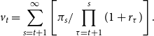 \begin{equation} v_{t}=\sum _{s=t+1}^{\infty }\left [ \pi _{s}/\prod \limits _{\tau =t+1}^{s}(1+r_{\tau })\right ] \text {.} \end{equation}
Competitive R&D entrepreneurs invent new products by employing $H_{R,t}$
units of human-capital-embodied labor. We specify the following innovation process:Footnote
15
$H_{R,t}$
units of human-capital-embodied labor. We specify the following innovation process:Footnote
15
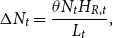 \begin{equation} \Delta N_{t}=\frac {\theta N_{t}H_{R,t}}{L_{t}}\text {,} \end{equation}
where $\Delta N_{t}\equiv N_{t+1}-N_{t}$
. The parameter
$\Delta N_{t}\equiv N_{t+1}-N_{t}$
. The parameter $\theta \gt 0$
determines R&D productivity
$\theta \gt 0$
determines R&D productivity $\theta N_{t}/L_{t}$
, where
$\theta N_{t}/L_{t}$
, where $N_{t}$
captures intertemporal knowledge spillovers as in Romer (Reference Romer1990) and
$N_{t}$
captures intertemporal knowledge spillovers as in Romer (Reference Romer1990) and $1/L_{t}$
captures a dilution effect that removes the scale effect.Footnote
16
If the following free-entry condition holds:
$1/L_{t}$
captures a dilution effect that removes the scale effect.Footnote
16
If the following free-entry condition holds:
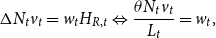 \begin{equation} \Delta N_{t}v_{t}=w_{t}H_{R,t}\Leftrightarrow \frac {\theta N_{t}v_{t}}{L_{t}}=w_{t}\text {,} \end{equation}
then R&D $H_{R,t}$
would be positive at time
$H_{R,t}$
would be positive at time $t$
. If
$t$
. If $\theta N_{t}v_{t}/L_{t}\lt w_{t}$
, then R&D does not take place at time
$\theta N_{t}v_{t}/L_{t}\lt w_{t}$
, then R&D does not take place at time $t$
(i.e.,
$t$
(i.e., $H_{R,t}=0$
). Lemma2 provides the condition for
$H_{R,t}=0$
). Lemma2 provides the condition for $H_{R,t}\gt 0$
, which requires R&D productivity
$H_{R,t}\gt 0$
, which requires R&D productivity $\theta$
to be sufficiently high in order for innovation to take place.
$\theta$
to be sufficiently high in order for innovation to take place.
Lemma 2.
R&D $H_{R,t}$
is positive at time
$H_{R,t}$
is positive at time $t$
if and only if the following inequality holds:
$t$
if and only if the following inequality holds:
 \begin{equation} \int _{0}^{1}\left [ 1-e_{t}(i)-\sigma n_{t}(i)\right ] h_{t}(i)s_{t}(i)di\gt \frac {1}{\theta }\text {.} \end{equation}
Proof. See Appendix A.
2.5 Aggregation
Imposing symmetry on (8) yields $Y_{t}=H_{Y,t}^{1-\alpha }N_{t}X_{t}^{\alpha }$
. Then, we substitute (10) and (12) into this equation to derive the aggregate production function as
$Y_{t}=H_{Y,t}^{1-\alpha }N_{t}X_{t}^{\alpha }$
. Then, we substitute (10) and (12) into this equation to derive the aggregate production function as
 \begin{equation} Y_{t}=\left ( \frac {\alpha }{\mu }\right ) ^{\alpha /(1-\alpha )}N_{t}H_{Y,t}\text {.} \end{equation}
Using $N_{t}X_{t}=(\alpha /\mu )Y_{t}$
, we obtain the following resource constraint on final good:
$N_{t}X_{t}=(\alpha /\mu )Y_{t}$
, we obtain the following resource constraint on final good:
 \begin{equation} C_{t}=Y_{t}-N_{t}X_{t}=\left ( 1-\frac {\alpha }{\mu }\right ) Y_{t}\text {,} \end{equation}
where $C_{t}$
denotes aggregate consumption. Finally, the resource constraint on human-capital-embodied labor is
$C_{t}$
denotes aggregate consumption. Finally, the resource constraint on human-capital-embodied labor is
 \begin{equation} \int _{0}^{1}\left [ 1-e_{t}(i)-\sigma n_{t}(i)\right ] h_{t}(i)L_{t}(i)di=H_{Y,t}+H_{R,t}\text {.} \end{equation}
2.6 Equilibrium
The equilibrium is a sequence of allocations $\{X_{t}(j),Y_{t},e_{t}(i),n_{t}(i),c_{t}(i),C_{t},h_{t}(i),H_{t},H_{Y,t},H_{R,t},L_{t}\}$
and prices
$\{X_{t}(j),Y_{t},e_{t}(i),n_{t}(i),c_{t}(i),C_{t},h_{t}(i),H_{t},H_{Y,t},H_{R,t},L_{t}\}$
and prices $\{p_{t}(j),w_{t},r_{t},v_{t}\}$
that satisfy the following conditions:
$\{p_{t}(j),w_{t},r_{t},v_{t}\}$
that satisfy the following conditions:
-
• individuals choose $\{e_{t}(i),n_{t}(i),c_{t}(i)\}$
to maximize utility taking
$\{r_{t+1},w_{t},h_{t}(i)\}$
as given;
$\{e_{t}(i),n_{t}(i),c_{t}(i)\}$
to maximize utility taking
$\{r_{t+1},w_{t},h_{t}(i)\}$
as given; -
• competitive firms produce
$Y_{t}$
to maximize profit taking
$\{p_{t}(j),w_{t}\}$
as given; -
• a monopolistic firm produces
$X_{t}(j)$
and chooses
$p_{t}(j)$
to maximize profit; -
• competitive entrepreneurs perform R&D to maximize profit taking
$\{w_{t},v_{t}\}$
as given; -
• the market-clearing condition for the final good holds such that
$Y_{t}=N_{t}X_{t}+C_{t}$
; -
• the resource constraint on human-capital-embodied labor holds such that
$H_{Y,t}+H_{R,t}=\int _{0}^{1}\left [ 1-e_{t}(i)-\sigma n_{t}(i)\right ] h_{t}(i)L_{t}(i)di$
; -
• total saving equals asset value such that
$w_{t}\int _{0}^{1}\left [ 1-e_{t}(i)-\sigma n_{t}(i)\right ] h_{t}(i)L_{t}(i)di=N_{t+1}v_{t}$
.


3. Stages of economic development
Our model features two stages of economic development. The first stage features only human capital accumulation. The second stage features both human capital accumulation and innovation.Footnote 17 The activation of innovation and the resulting transition from the first stage to the second stage are endogenous and do not always occur.
3.1 Stage 1: Human capital accumulation only
The initial level of human capital for each individual in household $i$
is
$i$
is $h_{0}(i)$
. Suppose the following inequality holds at time 0:
$h_{0}(i)$
. Suppose the following inequality holds at time 0:
 \begin{equation} \int _{0}^{1}\left [ 1-e_{0}(i)-\sigma n_{0}(i)\right ] h_{0}(i)s_{0}(i)di=\frac {1}{1+\eta +\gamma }\int _{0}^{1}\left [ 1+(1-\delta )\frac {h_{0}(i)}{\phi (i)}\right ] h_{0}(i)s_{0}(i)di\lt \frac {1}{\theta }\text {,} \end{equation}
which uses (4) and (5). In (21), both the initial labor share $s_{0}(i)\equiv L_{0}(i)/L_{0}$
and initial human capital
$s_{0}(i)\equiv L_{0}(i)/L_{0}$
and initial human capital $h_{0}(i)$
are exogenously given. Then, Lemma2 implies that
$h_{0}(i)$
are exogenously given. Then, Lemma2 implies that $H_{R,0}=0$
and
$H_{R,0}=0$
and
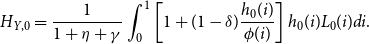 \begin{equation} H_{Y,0}=\frac {1}{1+\eta +\gamma }\int _{0}^{1}\left [ 1+(1-\delta )\frac {h_{0}(i)}{\phi (i)}\right ] h_{0}(i)L_{0}(i)di\text {.} \end{equation}
In this stage of development, the economy features only human capital accumulation. Human capital $h_{t}(i)$
accumulates according to the autonomous and stable dynamics in (6), and
$h_{t}(i)$
accumulates according to the autonomous and stable dynamics in (6), and $s_{t}(i)$
evolves according to Lemma1. However, so long as the following inequality holds at time
$s_{t}(i)$
evolves according to Lemma1. However, so long as the following inequality holds at time $t$
:
$t$
:
 \begin{equation} \int _{0}^{1}\left [ 1-e_{t}(i)-\sigma n_{t}(i)\right ] h_{t}(i)s_{t}(i)di=\frac {1}{1+\eta +\gamma }\int _{0}^{1}\left [ 1+(1-\delta )\frac {h_{t}(i)}{\phi (i)}\right ] h_{t}(i)s_{t}(i)di\lt \frac {1}{\theta }\text {,} \end{equation}
we continue to have $H_{R,t}=0$
and
$H_{R,t}=0$
and
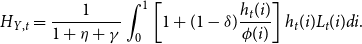 \begin{equation} H_{Y,t}=\frac {1}{1+\eta +\gamma }\int _{0}^{1}\left [ 1+(1-\delta )\frac {h_{t}(i)}{\phi (i)}\right ] h_{t}(i)L_{t}(i)di\text {.} \end{equation}
Substituting (24) into (18) yields the level of output per worker as
 \begin{equation} y_{t}\equiv \frac {Y_{t}}{L_{t}}=\left ( \frac {\alpha }{\mu }\right ) ^{\alpha /(1-\alpha )}N_{0}\frac {H_{Y,t}}{L_{t}}=\left ( \frac {\alpha }{\mu }\right ) ^{\alpha /(1-\alpha )}\frac {N_{0}}{1+\eta +\gamma }\int _{0}^{1}\left [ 1+(1-\delta )\frac {h_{t}(i)}{\phi (i)}\right ] h_{t}(i)s_{t}(i)di\text {,} \end{equation}
where $N_{0}$
remains at the initial level and output increases as human capital accumulates.
$N_{0}$
remains at the initial level and output increases as human capital accumulates.
3.2 Does innovation occur?
Equation (6) shows that human capital $h_{t}(i)$
converges to a steady state given by
$h_{t}(i)$
converges to a steady state given by
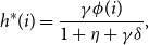 \begin{equation} h^{\ast }(i)=\frac {\gamma \phi (i)}{1+\eta +\gamma \delta }\text {,} \end{equation}
which is increasing in household $i$
’s ability
$i$
’s ability $\phi (i)$
. Substituting (26) into (4) and (5) yields the steady-state levels of education and fertility given by
$\phi (i)$
. Substituting (26) into (4) and (5) yields the steady-state levels of education and fertility given by
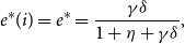 \begin{equation} e^{\ast }(i)=e^{\ast }=\frac {\gamma \delta }{1+\eta +\gamma \delta }\text {,} \end{equation}
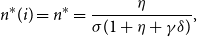 \begin{equation} n^{\ast }(i)=n^{\ast }=\frac {\eta }{\sigma (1+\eta +\gamma \delta )}\text {,} \end{equation}
where $n^{\ast }$
is the same across all households because they are independent of
$n^{\ast }$
is the same across all households because they are independent of $\phi (i)$
. In other words, the negative effect of
$\phi (i)$
. In other words, the negative effect of $\phi (i)$
and the positive effect of
$\phi (i)$
and the positive effect of $h^{\ast }(i)$
on
$h^{\ast }(i)$
on $n^{\ast }(i)$
cancel each other. As a result, the distribution of the population share of different households is stationary in the long run.
$n^{\ast }(i)$
cancel each other. As a result, the distribution of the population share of different households is stationary in the long run.
In the long run, we may have positive or negative population growth. If we assume $\eta \gt (1+\gamma \delta )\sigma /(1-\sigma )$
, then the long-run population growth rate would be positive (i.e.,
$\eta \gt (1+\gamma \delta )\sigma /(1-\sigma )$
, then the long-run population growth rate would be positive (i.e., $n^{\ast }\gt 1$
). If we assume
$n^{\ast }\gt 1$
). If we assume $\eta \lt (1+\gamma \delta )\sigma /(1-\sigma )$
instead, then the long-run population growth rate would be negative (i.e.,
$\eta \lt (1+\gamma \delta )\sigma /(1-\sigma )$
instead, then the long-run population growth rate would be negative (i.e., $n^{\ast }\lt 1$
). Even with negative population growth in the long run, the economy may still experience economic growth (i.e., long-run growth in
$n^{\ast }\lt 1$
). Even with negative population growth in the long run, the economy may still experience economic growth (i.e., long-run growth in $y_{t}$
) driven by innovation.Footnote
18
$y_{t}$
) driven by innovation.Footnote
18
Does innovation occur? It depends on R&D productivity $\theta$
. Lemma2 implies that if the following inequality holds:
$\theta$
. Lemma2 implies that if the following inequality holds:
 \begin{equation} \left ( 1-e^{\ast }-\sigma n^{\ast }\right ) \int _{0}^{1}h^{\ast }(i)s^{\ast }(i)di=\frac {\gamma }{(1+\eta +\gamma \delta )^{2}}\int _{0}^{1}\phi (i)s^{\ast }(i)di\gt \frac {1}{\theta }\text {,} \end{equation}
then human capital accumulation eventually triggers the activation of innovation, under which the R&D condition in (16) holds and R&D $H_{R,t}$
becomes positive. Therefore, the endogenous activation of innovation requires a sufficiently large R&D productivity parameter
$H_{R,t}$
becomes positive. Therefore, the endogenous activation of innovation requires a sufficiently large R&D productivity parameter $\theta$
, such that (29) holds before human capital converges to a steady state. If innovation does not occur, then the economy features only human capital accumulation and converges to the following steady-state level of output per worker:
$\theta$
, such that (29) holds before human capital converges to a steady state. If innovation does not occur, then the economy features only human capital accumulation and converges to the following steady-state level of output per worker:
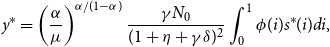 \begin{equation*} y^{\ast }=\left ( \frac {\alpha }{\mu }\right ) ^{\alpha /(1-\alpha )}\frac {\gamma N_{0}}{(1+\eta +\gamma \delta )^{2}}\int _{0}^{1}\phi (i)s^{\ast }(i)di\text {,} \end{equation*}
3.3 Stage 2: Innovation and human capital accumulation
We now consider the case in which the activation of innovation has occurred and derive the equilibrium growth rate in the presence of innovation. Substituting (18) into (9) yields the equilibrium wage rate as
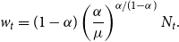 \begin{equation} w_{t}=(1-\alpha )\left ( \frac {\alpha }{\mu }\right ) ^{\alpha /(1-\alpha )}N_{t}\text {.} \end{equation}
Then, substituting (30) into (16) yields the equilibrium invention value as
 \begin{equation} \frac {v_{t}}{L_{t}}=\frac {1-\alpha }{\theta }\left ( \frac {\alpha }{\mu }\right ) ^{\alpha /(1-\alpha )}\text {.} \end{equation}
The structure of overlapping generations implies that the value of assets at the end of time $t$
must equal the amount of saving at time
$t$
must equal the amount of saving at time $t$
given by wage income at time
$t$
given by wage income at time $t$
:
$t$
:
 \begin{equation} N_{t+1}v_{t}=w_{t}\int _{0}^{1}\left [ 1-e_{t}(i)-\sigma n_{t}(i)\right ] h_{t}(i)L_{t}(i)di=w_{t}(H_{Y,t}+H_{R,t})\text {,} \end{equation}
where the second equality uses (20). Substituting (30) and (31) into (32) yields
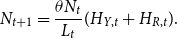 \begin{equation} N_{t+1}=\frac {\theta N_{t}}{L_{t}}(H_{Y,t}+H_{R,t})\text {.} \end{equation}
Combining (15) and (33) yields the equilibrium level of $H_{Y,t}$
as
$H_{Y,t}$
as
 \begin{equation} \frac {H_{Y,t}}{L_{t}}=\frac {1}{\theta } \end{equation}
for all $t$
. Substituting (4), (5) and (34) into (20) yields the equilibrium level of
$t$
. Substituting (4), (5) and (34) into (20) yields the equilibrium level of $H_{R,t}$
as
$H_{R,t}$
as
 \begin{align} \frac {H_{R,t}}{L_{t}}&=\int _{0}^{1}\left [ 1-e_{t}(i)-\sigma n_{t}(i)\right ] h_{t}(i)s_{t}(i)di-\frac {H_{Y,t}}{L_{t}}\\ \nonumber \quad &=\frac {1}{1+\eta +\gamma }\int _{0}^{1}\left [ 1+(1-\delta )\frac {h_{t}(i)}{\phi (i)}\right ] h_{t}(i)s_{t}(i)di-\frac {1}{\theta }\text {.} \end{align}
We can now substitute (35) into (15) to derive the equilibrium growth rate of $N_{t}$
as
$N_{t}$
as
 \begin{equation} g_{t}\equiv \frac {\Delta N_{t}}{N_{t}}=\frac {\theta H_{R,t}}{L_{t}}=\frac {\theta }{1+\eta +\gamma }\int _{0}^{1}\left [ 1+(1-\delta )\frac {h_{t}(i)}{\phi (i)}\right ] h_{t}(i)s_{t}(i)di-1\text {,} \end{equation}
which is also the equilibrium growth rate of output per worker $y_{t}=\left ( \alpha /\mu \right ) ^{\alpha /(1-\alpha )}N_{t}/\theta$
. Finally, the steady-state equilibrium growth rate of
$y_{t}=\left ( \alpha /\mu \right ) ^{\alpha /(1-\alpha )}N_{t}/\theta$
. Finally, the steady-state equilibrium growth rate of $N_{t}$
and
$N_{t}$
and $y_{t}$
is
$y_{t}$
is
 \begin{equation} g^{\ast }=\frac {\theta \gamma }{(1+\eta +\gamma \delta )^{2}}\int _{0}^{1}\phi (i)s^{\ast }(i)di-1\text {.} \end{equation}
In the steady state, $s^{\ast }(i)$
is also the population share of household
$s^{\ast }(i)$
is also the population share of household $i$
and still depends on the initial distribution of
$i$
and still depends on the initial distribution of $h_{0}(i)$
and the exogenous distribution of
$h_{0}(i)$
and the exogenous distribution of $\phi (i)$
as shown in Lemma1.
$\phi (i)$
as shown in Lemma1.
4. Heterogeneous households and evolutionary differences
Equation (21) shows that the activation of innovation-driven growth occurs at time 0 if and only if the following inequality holds:
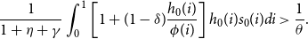 \begin{equation} \frac {1}{1+\eta +\gamma }\int _{0}^{1}\left [ 1+(1-\delta )\frac {h_{0}(i)}{\phi (i)}\right ] h_{0}(i)s_{0}(i)di\gt \frac {1}{\theta }\text {.} \end{equation}
Suppose we consider a useful benchmark of an equal initial labor share $s_{0}(i)=1$
and an equal initial level of human capital
$s_{0}(i)=1$
and an equal initial level of human capital $\ h_{0}(i)=h_{0}$
for all
$\ h_{0}(i)=h_{0}$
for all $i\in \lbrack 0,1]$
. Then, the left-hand side of (38) simplifies to
$i\in \lbrack 0,1]$
. Then, the left-hand side of (38) simplifies to
 \begin{equation} \frac {h_{0}}{1+\eta +\gamma }\left [ 1+(1-\delta )h_{0}\int _{0}^{1}\frac {1}{\phi (i)}di\right ] \gt \frac {h_{0}}{1+\eta +\gamma }\left [ 1+\frac {(1-\delta )h_{0}}{\overline {\phi }}\right ] \text {,} \end{equation}
where $\int _{0}^{1}[1/\phi (i)]di\gt 1/\overline {\phi }$
due to Jensen’s inequality. In other words, the presence of heterogeneity in
$\int _{0}^{1}[1/\phi (i)]di\gt 1/\overline {\phi }$
due to Jensen’s inequality. In other words, the presence of heterogeneity in $\phi (i)$
makes the activation of innovation-driven growth more likely to occur at time 0 than the absence of heterogeneity (i.e.,
$\phi (i)$
makes the activation of innovation-driven growth more likely to occur at time 0 than the absence of heterogeneity (i.e., $\phi (i)=\overline {\phi }$
for all
$\phi (i)=\overline {\phi }$
for all $i\in \lbrack 0,1]$
) does. Due to heterogeneity, some households supply more human capital for production and innovation while others supply less. Equation (39) implies that the former effect dominates the latter effect such that the initial amount of human capital available for production and innovation increases as a result of heterogeneity. The intuition can be explained as follows.
$i\in \lbrack 0,1]$
) does. Due to heterogeneity, some households supply more human capital for production and innovation while others supply less. Equation (39) implies that the former effect dominates the latter effect such that the initial amount of human capital available for production and innovation increases as a result of heterogeneity. The intuition can be explained as follows.
Although some low-ability households may devote almost no time to education and most of their time to work (and fertility), high-ability households always spend some time to work, as the following shows:
 \begin{equation*} 1-e_{0}(i)-\sigma n_{0}(i)=\frac {1}{1+\eta +\gamma }\left [ 1+\frac {(1-\delta )h_{0}}{\phi (i)}\right ] \gt \frac {1}{1+\eta +\gamma }\gt 0\text {.} \end{equation*}
The convexity of $1/\phi (i)$
in
$1/\phi (i)$
in $1-e_{0}(i)-\sigma n_{0}(i)$
gives rise to the positive effect of heterogeneity on the amount of human capital available for production and innovation. To put it differently, the low-ability households being less willing to educate their children contribute to a larger workforce, which in turn rewards the innovation pioneers with more profits extracted from a larger market size of the economy. We summarize this result in the following lemma.
$1-e_{0}(i)-\sigma n_{0}(i)$
gives rise to the positive effect of heterogeneity on the amount of human capital available for production and innovation. To put it differently, the low-ability households being less willing to educate their children contribute to a larger workforce, which in turn rewards the innovation pioneers with more profits extracted from a larger market size of the economy. We summarize this result in the following lemma.
Lemma 3. Heterogeneity makes it more likely for innovation to be activated at time 0.
Proof. If the following inequality holds:
 \begin{equation} \frac {h_{0}}{1+\eta +\gamma }\left [ 1+(1-\delta )h_{0}\int _{0}^{1}\frac {1}{\phi (i)}di\right ] \gt \frac {1}{\theta }\gt \frac {h_{0}}{1+\eta +\gamma }\left [ 1+\frac {(1-\delta )h_{0}}{\overline {\phi }}\right ] \text {,} \end{equation}
which is a nonempty parameter space due to $\int _{0}^{1}[1/\phi (i)]di\gt 1/\overline {\phi }$
, then the takeoff of the economy occurs at time 0 under heterogeneous households but not under homogeneous households.
$\int _{0}^{1}[1/\phi (i)]di\gt 1/\overline {\phi }$
, then the takeoff of the economy occurs at time 0 under heterogeneous households but not under homogeneous households.
Next we examine how the labor share of households evolves over time. Given the benchmark of an equal initial labor share $s_{0}(i)=1$
and an equal initial level of human capital
$s_{0}(i)=1$
and an equal initial level of human capital $\ h_{0}(i)=h_{0}$
for all
$\ h_{0}(i)=h_{0}$
for all $i\in \lbrack 0,1]$
, the fertility of household
$i\in \lbrack 0,1]$
, the fertility of household $i$
at time 0 is
$i$
at time 0 is
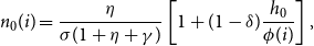 \begin{equation*} n_{0}(i)=\frac {\eta }{\sigma (1+\eta +\gamma )}\left [ 1+(1-\delta )\frac {h_{0}}{\phi (i)}\right ] \text {,} \end{equation*}
which is decreasing in $\phi (i)$
. For households with
$\phi (i)$
. For households with $\phi (i)\gt \overline {\phi }$
, their growth rate
$\phi (i)\gt \overline {\phi }$
, their growth rate $n_{0}(i)$
would be lower than
$n_{0}(i)$
would be lower than $n_{0}(\overline {\phi })$
. However, they will have a higher level of human capital in the next period:
$n_{0}(\overline {\phi })$
. However, they will have a higher level of human capital in the next period:
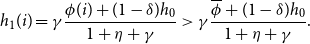 \begin{equation*} h_{1}(i)=\gamma \frac {\phi (i)+(1-\delta )h_{0}}{1+\eta +\gamma }\gt \gamma \frac {\overline {\phi }+(1-\delta )h_{0}}{1+\eta +\gamma }\text {.} \end{equation*}
This higher level of human capital gives rise to a higher growth rate $n_{1}(i)$
and reduces the difference between
$n_{1}(i)$
and reduces the difference between $n_{1}(i)$
and
$n_{1}(i)$
and $n_{1}(\overline {\phi })$
. However, as shown in Lemma1,
$n_{1}(\overline {\phi })$
. However, as shown in Lemma1, $n_{t}(i)$
remains lower than
$n_{t}(i)$
remains lower than $n_{t}(\overline {\phi })$
for
$n_{t}(\overline {\phi })$
for $\phi (i)\gt \overline {\phi }$
until
$\phi (i)\gt \overline {\phi }$
until $h_{t}(i)$
converges to its steady-state level in (26) at which point the population growth rate of all households
$h_{t}(i)$
converges to its steady-state level in (26) at which point the population growth rate of all households $i\in \lbrack 0,1]$
converges to
$i\in \lbrack 0,1]$
converges to $n^{\ast }$
in (28). Therefore, the population growth rates of households with
$n^{\ast }$
in (28). Therefore, the population growth rates of households with $\phi (i)\gt \overline {\phi }$
are lower than the population growth rates of households with
$\phi (i)\gt \overline {\phi }$
are lower than the population growth rates of households with $\phi (i)\lt \overline {\phi }$
until
$\phi (i)\lt \overline {\phi }$
until $h_{t}(i)$
converges to its steady-state level in (26). This temporary evolutionary disadvantage of high-ability households will never be compensated despite population trends being equal across households in the long run.
$h_{t}(i)$
converges to its steady-state level in (26). This temporary evolutionary disadvantage of high-ability households will never be compensated despite population trends being equal across households in the long run.
The above analysis implies that there exists a threshold for $\phi (i)$
above (below) which
$\phi (i)$
above (below) which $s^{\ast }(i)\lt 1$
(
$s^{\ast }(i)\lt 1$
( $s^{\ast }(i)\gt 1$
). This in turn implies thatFootnote
19
$s^{\ast }(i)\gt 1$
). This in turn implies thatFootnote
19
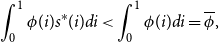 \begin{equation} \int _{0}^{1}\phi (i)s^{\ast }(i)di\lt \int _{0}^{1}\phi (i)di=\overline {\phi }\text {,} \end{equation}
because the households with larger $\phi (i)$
end up having a lower steady-state population share
$\phi (i)$
end up having a lower steady-state population share $s^{\ast }(i)$
. Therefore, we also have the following inequality:
$s^{\ast }(i)$
. Therefore, we also have the following inequality:
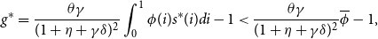 \begin{equation} g^{\ast }=\frac {\theta \gamma }{(1+\eta +\gamma \delta )^{2}}\int _{0}^{1}\phi (i)s^{\ast }(i)di-1\lt \frac {\theta \gamma }{(1+\eta +\gamma \delta )^{2}}\overline {\phi }-1\text {,} \end{equation}
where the right-hand side of the inequality is the steady-state innovation-driven growth rate under homogeneous households (i.e., $\phi (i)=\overline {\phi }$
for all
$\phi (i)=\overline {\phi }$
for all $i\in \lbrack 0,1]$
) in an economy that has experienced the transition to innovation. In other words, the steady-state growth rate
$i\in \lbrack 0,1]$
) in an economy that has experienced the transition to innovation. In other words, the steady-state growth rate $g^{\ast }$
becomes lower because the heterogeneity in households and the temporary evolutionary disadvantage of the high-ability households reduce the average level of human capital and consequently the rate of innovation (recall that
$g^{\ast }$
becomes lower because the heterogeneity in households and the temporary evolutionary disadvantage of the high-ability households reduce the average level of human capital and consequently the rate of innovation (recall that $g_{t}=\theta H_{R,t}/L_{t}$
) in the long run. We summarize the above result in the following proposition.
$g_{t}=\theta H_{R,t}/L_{t}$
) in the long run. We summarize the above result in the following proposition.
Proposition 1.
The temporary evolutionary disadvantage of the high-ability households causes a lower steady-state equilibrium growth rate $g^{\ast }$
than the case of homogeneous households without natural selection.
$g^{\ast }$
than the case of homogeneous households without natural selection.
Proof. See Appendix A.
4.1 A parametric example
In this section, we provide a simple parametric example to illustrate our results more clearly and prepare for the empirical analysis in Section 5. We consider two types of households. Specifically, $\phi (i)=\overline {\phi }+\varsigma$
for
$\phi (i)=\overline {\phi }+\varsigma$
for $i\in \lbrack 0,0.5]$
and
$i\in \lbrack 0,0.5]$
and $\phi (j)=\overline {\phi }-\varsigma$
for
$\phi (j)=\overline {\phi }-\varsigma$
for $j\in \lbrack 0.5,1]$
. As before, the households own the same initial amount of human capital (i.e.,
$j\in \lbrack 0.5,1]$
. As before, the households own the same initial amount of human capital (i.e., $h_{0}(i)=h_{0}$
for
$h_{0}(i)=h_{0}$
for $i\in \lbrack 0,1]$
). Their initial population shares are also the same (i.e.,
$i\in \lbrack 0,1]$
). Their initial population shares are also the same (i.e., $s_{0}(i)=1$
for
$s_{0}(i)=1$
for $i\in \lbrack 0,1]$
); in this case, the mean of
$i\in \lbrack 0,1]$
); in this case, the mean of $\phi (i)$
is simply
$\phi (i)$
is simply $\overline {\phi }$
and the coefficient of variation in
$\overline {\phi }$
and the coefficient of variation in $\phi (i)$
is
$\phi (i)$
is $\varsigma /\overline {\phi }$
. Therefore, for a given
$\varsigma /\overline {\phi }$
. Therefore, for a given $\overline {\phi }$
, an increase in
$\overline {\phi }$
, an increase in $\varsigma$
raises the coefficient of variation in
$\varsigma$
raises the coefficient of variation in $\phi (i)$
and also makes (40) more likely to hold by raising
$\phi (i)$
and also makes (40) more likely to hold by raising $\int _{0}^{1}[1/\phi (i)]di=1/(\overline {\phi }-\varsigma ^{2}/\overline {\phi })\gt 1/\overline {\phi }$
.
$\int _{0}^{1}[1/\phi (i)]di=1/(\overline {\phi }-\varsigma ^{2}/\overline {\phi })\gt 1/\overline {\phi }$
.
From (26), their steady-state levels of human capital are different and given by $h^{\ast }(i)=\gamma (\overline {\phi }+\varsigma )/(1+\eta +\gamma \delta )$
for
$h^{\ast }(i)=\gamma (\overline {\phi }+\varsigma )/(1+\eta +\gamma \delta )$
for $i\in \lbrack 0,0.5]$
and
$i\in \lbrack 0,0.5]$
and $h^{\ast }(j)=\gamma (\overline {\phi }-\varsigma )/(1+\eta +\gamma \delta )$
for
$h^{\ast }(j)=\gamma (\overline {\phi }-\varsigma )/(1+\eta +\gamma \delta )$
for $j\in \lbrack 0.5,1]$
. From (42), the steady-state growth rate
$j\in \lbrack 0.5,1]$
. From (42), the steady-state growth rate $g^{\ast }$
is given by
$g^{\ast }$
is given by
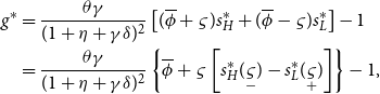 \begin{align} g^{\ast }&=\frac {\theta \gamma }{(1+\eta +\gamma \delta )^{2}}\left [ (\overline {\phi }+\varsigma )s_{H}^{\ast }+(\overline {\phi }-\varsigma )s_{L}^{\ast }\right ] -1\\ \nonumber \quad &=\frac {\theta \gamma }{(1+\eta +\gamma \delta )^{2}}\left \{ \overline {\phi }+\varsigma \left [ s_{H}^{\ast }(\underset {-}{\varsigma })-s_{L}^{\ast }(\underset {+}{\varsigma })\right ] \right \} -1\text {,} \end{align}
where $s_{L}^{\ast }\equiv \int _{0.5}^{1}s^{\ast }(j)dj=s^{\ast }(j)/2$
is the steady-state population share of household
$s_{L}^{\ast }\equiv \int _{0.5}^{1}s^{\ast }(j)dj=s^{\ast }(j)/2$
is the steady-state population share of household $j\in \lbrack 0.5,1]$
with low ability
$j\in \lbrack 0.5,1]$
with low ability $\phi (j)=\overline {\phi }-\varsigma$
whereas
$\phi (j)=\overline {\phi }-\varsigma$
whereas $s_{H}^{\ast }\equiv \int _{0}^{0.5}s^{\ast }(i)di=s^{\ast }(i)/2$
is the steady-state population share of household
$s_{H}^{\ast }\equiv \int _{0}^{0.5}s^{\ast }(i)di=s^{\ast }(i)/2$
is the steady-state population share of household $i\in \lbrack 0,0.5]$
with high ability
$i\in \lbrack 0,0.5]$
with high ability $\phi (i)=\overline {\phi }+\varsigma$
. We note that
$\phi (i)=\overline {\phi }+\varsigma$
. We note that $s_{H}^{\ast }+s_{L}^{\ast }=1$
. Then, from Lemma1, we have
$s_{H}^{\ast }+s_{L}^{\ast }=1$
. Then, from Lemma1, we have
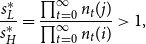 \begin{equation} \frac {s_{L}^{\ast }}{s_{H}^{\ast }}=\frac {\prod \nolimits _{t=0}^{\infty }n_{t}(j)}{\prod \nolimits _{t=0}^{\infty }n_{t}(i)}\gt 1\text {,} \end{equation}
where
 \begin{eqnarray*} n_{t}(j) &=&\frac {\eta }{\sigma (1+\eta +\gamma )}\left \{ \sum _{\tau =0}^{t-1}\left [ \frac {\gamma (1-\delta )}{1+\eta +\gamma }\right ] ^{\tau }+\left [ \frac {\gamma (1-\delta )}{1+\eta +\gamma }\right ] ^{t}\left [ 1+(1-\delta )\frac {h_{0}}{\overline {\phi }-\varsigma }\right ] \right \} \text {,} \\ n_{t}(i) &=&\frac {\eta }{\sigma (1+\eta +\gamma )}\left \{ \sum _{\tau =0}^{t-1}\left [ \frac {\gamma (1-\delta )}{1+\eta +\gamma }\right ] ^{\tau }+\left [ \frac {\gamma (1-\delta )}{1+\eta +\gamma }\right ] ^{t}\left [ 1+(1-\delta )\frac {h_{0}}{\overline {\phi }+\varsigma }\right ] \right \} \text {.} \end{eqnarray*}
Therefore, $s_{L}^{\ast }/s_{H}^{\ast }$
is increasing in
$s_{L}^{\ast }/s_{H}^{\ast }$
is increasing in $\varsigma$
, which together with
$\varsigma$
, which together with $s_{H}^{\ast }+s_{L}^{\ast }=1$
implies that
$s_{H}^{\ast }+s_{L}^{\ast }=1$
implies that $s_{L}^{\ast }$
is increasing in
$s_{L}^{\ast }$
is increasing in $\varsigma$
and
$\varsigma$
and $s_{H}^{\ast }$
is decreasing in
$s_{H}^{\ast }$
is decreasing in $\varsigma$
as stated in (43).
$\varsigma$
as stated in (43).
In summary, an increase in $\varsigma$
leads to an immediate increase in the coefficient of variation in
$\varsigma$
leads to an immediate increase in the coefficient of variation in $\phi (i)$
given by
$\phi (i)$
given by $\varsigma /\overline {\phi }$
and a subsequent decrease in the steady-state growth rate
$\varsigma /\overline {\phi }$
and a subsequent decrease in the steady-state growth rate $g^{\ast }$
given by (43) by reducing the average level of human capital and the level of innovation in the long run due to the temporary evolutionary disadvantage of the high-ability households. In the next section, we will test this theoretical prediction using cross-country data.
$g^{\ast }$
given by (43) by reducing the average level of human capital and the level of innovation in the long run due to the temporary evolutionary disadvantage of the high-ability households. In the next section, we will test this theoretical prediction using cross-country data.
Corollary 1.
Raising $\varsigma$
causes a larger coefficient of variation in
$\varsigma$
causes a larger coefficient of variation in $\phi (i)$
and a lower steady-state growth rate
$\phi (i)$
and a lower steady-state growth rate $g^{\ast }$
.
$g^{\ast }$
.
4.1.1 Education policy
We now consider a simple policy experiment. Suppose the government designs a set of policies (which may be public investment in education or an institutional reform in the education system) that improve the schooling system for all households. If these policies are nondiscriminatory, then we can treat them as a proportional shock $\lambda _{e}\gt 1$
that scales up the education abilities
$\lambda _{e}\gt 1$
that scales up the education abilities $\phi (i)$
of all households. High-ability households’ ability will become
$\phi (i)$
of all households. High-ability households’ ability will become $\lambda _{e}\left ( \overline {\phi }+\varsigma \right )$
, whereas low-ability households’ ability will become
$\lambda _{e}\left ( \overline {\phi }+\varsigma \right )$
, whereas low-ability households’ ability will become $\lambda _{e}\left ( \overline {\phi }-\varsigma \right )$
. Since
$\lambda _{e}\left ( \overline {\phi }-\varsigma \right )$
. Since $\overline {\phi }-\varsigma \gt 0$
, the effects on fertility
$\overline {\phi }-\varsigma \gt 0$
, the effects on fertility $n_{t}(j)$
and
$n_{t}(j)$
and $n_{t}(i)$
are all negative. This result means that education facilities and support will reduce population growth by increasing the family’s potential for education. For example, after decades of education policies, China’s fertility rate has dropped despite the 2016 abandonment of the single-child policy. Our model allows arguing that China’s recent population decline is not easily revertible because the country’s fertility transition to quality children is a byproduct of its inclusive and meritocratic education tradition. Will it hamper economic growth? According to our model, it will not. The reader can easily prove that
$n_{t}(i)$
are all negative. This result means that education facilities and support will reduce population growth by increasing the family’s potential for education. For example, after decades of education policies, China’s fertility rate has dropped despite the 2016 abandonment of the single-child policy. Our model allows arguing that China’s recent population decline is not easily revertible because the country’s fertility transition to quality children is a byproduct of its inclusive and meritocratic education tradition. Will it hamper economic growth? According to our model, it will not. The reader can easily prove that
 \begin{equation*} \frac {1+(1-\delta )\frac {h_{0}}{\lambda _{e}\left ( \overline {\phi }-\varsigma \right ) }}{1+(1-\delta )\frac {h_{0}}{\lambda _{e}\left ( \overline {\phi }+\varsigma \right ) }} \end{equation*}
decreases in $\lambda _{e}$
, which implies - by (44) - that
$\lambda _{e}$
, which implies - by (44) - that $s_{L}^{\ast }/s_{H}^{\ast }$
decreases as well, thereby leading to an increase in
$s_{L}^{\ast }/s_{H}^{\ast }$
decreases as well, thereby leading to an increase in $g^{\ast }$
due to the evolutionary process giving rise to a larger population share of high-ability households. Therefore, we can state that:
$g^{\ast }$
due to the evolutionary process giving rise to a larger population share of high-ability households. Therefore, we can state that:
Corollary 2. A policy that proportionally raises all education abilities will lead to a decrease in fertility and an increase in long-term economic growth.
5. EMPIRICAL EVIDENCE
The main theoretical prediction of this study hinges on the quality-quantity tradeoff in fertility, a concept extensively explored by Galor (Reference Galor2005, Reference Galor2011, Reference Galor2022) and others in related literature.Footnote 20 This tradeoff is rooted in parents’ decisions about their children’s education: providing education requires time and resources, which limits the number of children they can effectively support. This tradeoff implies that households with higher educational attainment experience an evolutionary disadvantage, leading to a smaller population share over time. This observation is consistent with our model, where households with higher abilities generally possess greater human capital and lower fertility rates, creating a negative relationship between these two endogenous variables.
Corollary1 of our theoretical model predicts that the negative relationship between fertility and education leads to a detrimental impact of heterogeneity in human capital accumulation on economic growth. To empirically test this prediction, we utilize cross-country data, with global standardized tests of students’ academic performance serving as proxies for educational ability. Specifically, we focus on the Trends in International Mathematics and Science Study (TIMSS), a widely recognized assessment of student performance in mathematics and science across the globe. From this data, we calculate the coefficient of variation of scores within each country as a measure of the heterogeneity in educational ability.
TIMSS indicators, being standardized, allow for direct cross-country comparisons.Footnote 21 We focus on fourth-grade students, as this group provides a more representative sample of nationwide educational differences compared to ninth-grade students. Prior research by Angrist et al. (Reference Angrist, Djankov, Goldberg and Patrinos2021) has shown that overall student performance varies minimally over time, but significant differences persist across countries. Similarly, the coefficient of variation in TIMSS scores changes little over time but exhibits substantial cross-country variation, making it a robust measure for analyzing the impact of educational ability heterogeneity at the national level.Footnote 22
To address potential omitted variable bias, we include controls for cultural characteristics such as time preference, which could influence both the independent and dependent variables. Specifically, we use the average level of long-term orientation in a country, following Hofstede (Reference Hofstede1991) and Galor and Özak (Reference Galor and Özak2016).Footnote 23 We also incorporate a comprehensive set of geographic variables, as suggested by Arbatlı et al. (Reference Arbatlı, Ashraf, Galor and Klemp2020),Footnote 24 including factors such as distance from the equator, proximity to waterways, and land suitability for agriculture, all of which have been shown to influence economic development.
Our analysis focuses on 67 countries that participated in the TIMSS tests, examining the impact of educational ability heterogeneity on economic growth from 1951 to 2017. The regression equation is specified as follows:
 \begin{equation*} y_{i,t}=\beta _{0}+\beta _{1}\text {var}_{i}+\gamma Z_{i}+\varphi _{t}+\varphi _{c}+\epsilon _{i,t}\text {,} \end{equation*}
where (i) $y_{i,t}$
represents economic growth of country
$y_{i,t}$
represents economic growth of country $i$
at time
$i$
at time $t$
, measured by the annual growth rate of GDP per capita; (ii) the independent variable
$t$
, measured by the annual growth rate of GDP per capita; (ii) the independent variable $\text {var}_{i}$
captures the heterogeneity of educational ability in country
$\text {var}_{i}$
captures the heterogeneity of educational ability in country $i$
, using the coefficient of variation of TIMSS scores;Footnote
25
(iii)
$i$
, using the coefficient of variation of TIMSS scores;Footnote
25
(iii) $Z_{i}$
includes controls for time preference and geographical characteristics (e.g., distance to the nearest waterway, absolute latitude, mean elevation, and agricultural land suitability, standard deviation in elevation and agricultural land suitability, and an island dummy);Footnote
26
and (iv)
$Z_{i}$
includes controls for time preference and geographical characteristics (e.g., distance to the nearest waterway, absolute latitude, mean elevation, and agricultural land suitability, standard deviation in elevation and agricultural land suitability, and an island dummy);Footnote
26
and (iv) $\varphi _{t}$
and
$\varphi _{t}$
and $\varphi _{c}$
are year fixed effects and continent fixed effects, respectively. We provide the summary statistics in Appendix C. In Corollary1, our theoretical framework predicts that a larger coefficient of variation in ability induces a lower steady-state growth rate, which implies
$\varphi _{c}$
are year fixed effects and continent fixed effects, respectively. We provide the summary statistics in Appendix C. In Corollary1, our theoretical framework predicts that a larger coefficient of variation in ability induces a lower steady-state growth rate, which implies $\beta _{1}\lt 0$
.
$\beta _{1}\lt 0$
.
5.1 Empirical results
Table 1 presents the results from our baseline cross-country analysis. Column 1 starts with a bivariate regression, showing that educational ability heterogeneity is negatively and significantly associated with GDP per capita growth rates. This relationship is visually depicted in Figure 2 of Appendix C, where we plot average annual economic growth rates against educational ability heterogeneity across countries. The scatter plot clearly illustrates a negative relationship, observed across various continents, as indicated by distinct color-coded data points.
Table 1. Heterogeneity of educational ability and economic growth
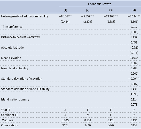
Notes: *** p $\lt$
0.01, ** p
$\lt$
0.01, ** p $\lt$
0.05, * p
$\lt$
0.05, * p $\lt$
0.1. Standard errors in parentheses are clustered by country. The dependent variable is the growth rate of GDP per capita.
$\lt$
0.1. Standard errors in parentheses are clustered by country. The dependent variable is the growth rate of GDP per capita.
To ensure the robustness of our findings, we progressively introduce additional controls. Column 2 adds year fixed effects to account for time-varying factors, while Column 3 incorporates continent fixed effects to control for regional differences. The baseline model presented in Column 4 includes controls for time preferences, geographical characteristics such as proximity to waterways, absolute latitude, mean and standard deviation of elevation, mean and standard deviation of land suitability, and an island dummy.
Despite these controls, concerns about endogeneity remain. The heterogeneity of educational ability and the spatial distribution of economic growth could be jointly influenced by unobserved cultural, institutional, or human factors. For instance, in societies that highly value education, individuals might strive for academic excellence, leading to less variation in test scores and faster economic growth. Ignoring these unobserved factors could bias our results. To address this, we employ two instrumental variables: ancestry adjusted population diversity and migratory distance from East Africa.
Table 2. Impacts of heterogeneity of educational ability using instrumental variables
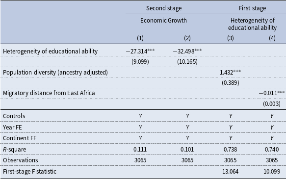
Note: p $\lt$
0.01, ** p
$\lt$
0.01, ** p $\lt$
0.05, * p
$\lt$
0.05, * p $\lt$
0.1. Standard errors in parentheses are clustered by country. The dependent variables in columns 1 and 2 are the growth rate of GDP per capita. Column 1 shows the second-stage results using population diversity (ancestry adjusted) as the instrumental variable, with the corresponding first-stage results presented in Column 3. Column 2 presents the second-stage results using prehistoric migratory distance from East Africa as the instrumental variable, with the corresponding first-stage results shown in Column 4. Controls include time preference, distance to the nearest waterway, absolute latitude, mean elevation, mean agricultural land suitability, standard deviation in elevation, standard deviation in agricultural land suitability, and an island dummy.
$\lt$
0.1. Standard errors in parentheses are clustered by country. The dependent variables in columns 1 and 2 are the growth rate of GDP per capita. Column 1 shows the second-stage results using population diversity (ancestry adjusted) as the instrumental variable, with the corresponding first-stage results presented in Column 3. Column 2 presents the second-stage results using prehistoric migratory distance from East Africa as the instrumental variable, with the corresponding first-stage results shown in Column 4. Controls include time preference, distance to the nearest waterway, absolute latitude, mean elevation, mean agricultural land suitability, standard deviation in elevation, standard deviation in agricultural land suitability, and an island dummy.
Ancestry-adjusted population diversity, as discussed by Ashraf and Galor (Reference Ashraf and Galor2013) and Arbatlı et al. (Reference Arbatlı, Ashraf, Galor and Klemp2020), relates to differences in educational ability and is exogenous to contemporary economic conditions. Migratory distance from East Africa that was used in previous studies, such as Ashraf and Galor (Reference Ashraf and Galor2013), Arbatlı et al. (Reference Arbatlı, Ashraf, Galor and Klemp2020), Ashraf et al. (Reference Ashraf, Galor and Klemp2021) and Galor et al. (Reference Galor, Klemp and Wainstock2023), captures the historical migration patterns that shaped genetic diversity, which could influence educational ability heterogeneity.
Table 2 presents the results of the two-stage least squares (2SLS) regressions. In the second stage, Columns 1 and 2 show that the coefficient for educational ability heterogeneity remains significantly negative, confirming its detrimental impact on economic growth. The first-stage results in Columns 3 and 4 validate our instruments, showing a significant positive correlation between educational ability heterogeneity and ancestry adjusted population diversity, and a significant negative correlation with migratory distance from East Africa.
Next, we consider education and innovation as alternative proxies for economic growth. In Columns 1 and 2 of Table 3, the dependent variables are the share of the population with at least some primary education and the logarithm of the average years of education, respectively, capturing the average education level. Columns 3 and 4 use the logarithm of the number of researchers in R&D (per million people) and the logarithm of patent applications as dependent variables, representing innovation rates. The negative coefficients for educational ability heterogeneity across these specifications suggest that it adversely affects both education and innovation, further supporting our theoretical predictions.Footnote 27 We have also conducted several robustness checks to affirm the reliability of our findings.Footnote 28
Table 3. Impacts of heterogeneity of educational ability on education and innovation
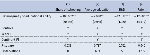
Note: p $\lt$
0.01, ** p
$\lt$
0.01, ** p $\lt$
0.05, * p
$\lt$
0.05, * p $\lt$
0.1. Standard errors in parentheses are clustered by country. In columns 1–2, the dependent variables are the share of the population with primary schooling and the log of average years of education in the first two columns, respectively. In columns 3–4, the dependent variables are the log of the number of researchers in R&D (per million people) and the log of the number of patent applications, respectively. Controls include time preference, distance to the nearest waterway, absolute latitude, mean elevation, mean agricultural land suitability, standard deviation in elevation and agricultural land suitability, and an island dummy.
$\lt$
0.1. Standard errors in parentheses are clustered by country. In columns 1–2, the dependent variables are the share of the population with primary schooling and the log of average years of education in the first two columns, respectively. In columns 3–4, the dependent variables are the log of the number of researchers in R&D (per million people) and the log of the number of patent applications, respectively. Controls include time preference, distance to the nearest waterway, absolute latitude, mean elevation, mean agricultural land suitability, standard deviation in elevation and agricultural land suitability, and an island dummy.
6. Conclusion
In this study, we developed an innovation-driven growth model with endogenous takeoff and fertility, offering new insights into the natural selection of heterogeneous households differentiated by their ability to accumulate human capital. Our key findings can be summarized as follows.
In the short run, we demonstrate the emergence of a “survival-of-the-weakest” scenario, where households with higher abilities actually face a temporary evolutionary disadvantage. This disadvantage is eventually mitigated as human capital accumulates. However, in the long run, this temporary setback for high-ability households has enduring negative effects on R&D, technological progress, and long-term economic growth.
Empirically, our cross-country analysis supports the model’s predictions, highlighting the detrimental impact of educational heterogeneity on long-term outcomes in education, innovation, and economic growth. While we employ instrumental variables to address potential endogeneity concerns, we acknowledge that these methods may not fully eliminate the issue. Nevertheless, the robustness of our findings across various specifications reinforces the validity of our theoretical predictions.
Theoretically, our work makes a significant contribution by introducing the concept of natural selection among heterogeneous households into the framework of the innovation-driven growth model. This addition enriches the existing literature on economic growth by providing a more nuanced understanding of how demographic dynamics and human capital accumulation interact with innovation processes.
While our model offers valuable insights, it also opens up several avenues for future research. A particularly promising direction would be to explore the policy implications of our findings in greater detail. Investigating how government interventions or institutional reforms might influence the interplay between natural selection, human capital accumulation, and economic growth could enhance the practical relevance of our model.
Additionally, integrating other socioeconomic factors—such as cultural attitudes, as explored by Cozzi (Reference Cozzi1998) and Tabellini (Reference Tabellini2010), or the dynamics of preference transmission, as discussed by Bisin and Verdier (Reference Bisin and Verdier1998, Reference Bisin and Verdier2000, Reference Bisin and Verdier2001, Reference Bisin and Verdier2017)—could add further depth and realism to the theory. Exploring these extensions could yield valuable insights into how the subtle dynamics of natural selection within heterogeneous households shape macroeconomic outcomes.
In conclusion, our study not only advances the understanding of innovation-driven growth, endogenous takeoff, and natural selection but also raises important questions for future research. By emphasizing the complex interactions between human capital, fertility choices, and economic development, we contribute to a more comprehensive understanding of the multifaceted nature of economic growth.
Acknowledgements
The authors are most grateful to Oded Galor for helpful advice and also would like to thank the Associate Editor and Referees for insightful comments. The usual disclaimer applies.
Funding statement
Chu gratefully acknowledges financial support from the Asia-Pacific Academy of Economics and Management at the University of Macau. Fan acknowledges financial support from the National Natural Science Foundation of China (72373030, 72433002, and 72341008).
Appendix A: Proofs
Proof of Lemma 1. The labor share of household $i$
is
$i$
is $s_{t}(i)\equiv L_{t}(i)/L_{t}$
, where
$s_{t}(i)\equiv L_{t}(i)/L_{t}$
, where
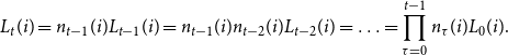 \begin{equation} L_{t}(i)=n_{t-1}(i)L_{t-1}(i)=n_{t-1}(i)n_{t-2}(i)L_{t-2}(i)=\ldots =\prod \limits _{\tau =0}^{t-1}n_{\tau }(i)L_{0}(i)\text {.} \end{equation}
From (4), the fertility choice at time 0 is given by
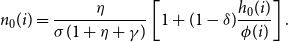 \begin{equation} n_{0}(i)=\frac {\eta }{\sigma (1+\eta +\gamma )}\left [ 1+(1-\delta )\frac { h_{0}(i)}{\phi (i)}\right ] \text {.} \end{equation}
From (6), the level of human capital at time 1 is given by
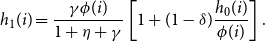 \begin{equation} h_{1}(i)=\frac {\gamma \phi (i)}{1+\eta +\gamma }\left [ 1+(1-\delta )\frac { h_{0}(i)}{\phi (i)}\right ] \text {.} \end{equation}
Substituting (A3) into (4) yields the fertility choice at time 1 as
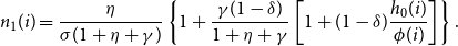 \begin{equation} n_{1}(i)=\frac {\eta }{\sigma (1+\eta +\gamma )}\left \{ 1+\frac {\gamma (1-\delta )}{1+\eta +\gamma }\left [ 1+(1-\delta )\frac {h_{0}(i)}{\phi (i)} \right ] \right \} \text {.} \end{equation}
Substituting (A3) into (6) yields the level of human capital at time 2 as
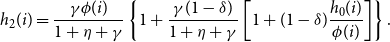 \begin{equation} h_{2}(i)=\frac {\gamma \phi (i)}{1+\eta +\gamma }\left \{ 1+\frac {\gamma (1-\delta )}{1+\eta +\gamma }\left [ 1+(1-\delta )\frac {h_{0}(i)}{\phi (i)} \right ] \right \} \text {.} \end{equation}
Substituting (A5) into (4) yields the fertility choice at time 2 as
 \begin{equation} n_{2}(i)=\frac {\eta }{\sigma (1+\eta +\gamma )}\left \{ 1+\frac {\gamma (1-\delta )}{1+\eta +\gamma }+\left [ \frac {\gamma (1-\delta )}{1+\eta +\gamma }\right ] ^{2}\left [ 1+(1-\delta )\frac {h_{0}(i)}{\phi (i)}\right ] \right \} \text {.} \end{equation}
Then, we can continue the process to derive the fertility choice at time $t\geq 3$
as
$t\geq 3$
as
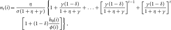 \begin{align} n_{t}(i)&=\frac {\eta }{\sigma (1+\eta +\gamma )}\left \{ 1+\frac {\gamma (1-\delta )}{1+\eta +\gamma }+\ldots +\left [ \frac {\gamma (1-\delta )}{1+\eta +\gamma }\right ] ^{t-1}+\left [ \frac {\gamma (1-\delta )}{1+\eta +\gamma } \right ] ^{t} \right. \nonumber \\ & \qquad \left. \left [ 1+(1-\delta )\frac {h_{0}(i)}{\phi (i)}\right ] \right \} \text {,} \end{align}
which can then be re-expressed using a summation sign as in Lemma1.
Proof of Lemma 2. If (17) holds, then (35) shows that $H_{R,t}\gt 0$
. Now, let’s consider the case in which
$H_{R,t}\gt 0$
. Now, let’s consider the case in which
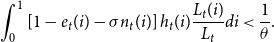 \begin{equation} \int _{0}^{1}\left [ 1-e_{t}(i)-\sigma n_{t}(i)\right ] h_{t}(i)\frac {L_{t}(i)}{ L_{t}}di\lt \frac {1}{\theta }\text {.} \end{equation}
Recall that the value of assets at the end of time $t$
must equal the amount of saving at time
$t$
must equal the amount of saving at time $t$
given by wage income at time
$t$
given by wage income at time $t$
such that
$t$
such that
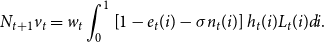 \begin{equation} N_{t+1}v_{t}=w_{t}\int _{0}^{1}\left [ 1-e_{t}(i)-\sigma n_{t}(i)\right ] h_{t}(i)L_{t}(i)di\text {.} \end{equation}
Substituting (A9) into (A8) yields
 \begin{equation} w_{t}\gt \frac {\theta N_{t+1}v_{t}}{L_{t}}\geq \frac {\theta N_{t}v_{t}}{L_{t}} \text {,} \end{equation}
where the second inequality uses $N_{t+1}\geq N_{t}$
. Equation (A10) implies that
$N_{t+1}\geq N_{t}$
. Equation (A10) implies that $\Delta N_{t}v_{t}=w_{t}H_{R,t}$
in (16) cannot hold unless
$\Delta N_{t}v_{t}=w_{t}H_{R,t}$
in (16) cannot hold unless $H_{R,t}=0$
.
$H_{R,t}=0$
.
Proof of Proposition 1. From Lemma1, the steady-state population share of household $i$
is given by
$i$
is given by
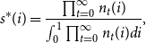 \begin{equation} s^{\ast }(i)=\frac {\prod \nolimits _{t=0}^{\infty }n_{t}(i)}{\int _{0}^{1}\prod \nolimits _{t=0}^{\infty }n_{t}(i)di}\text {,} \end{equation}
where we have used $L_{0}(i)=L_{0}$
for all
$L_{0}(i)=L_{0}$
for all $i$
. Lemma1 shows that
$i$
. Lemma1 shows that $n_{t}(i)$
is monotonically decreasing in
$n_{t}(i)$
is monotonically decreasing in $\phi (i)$
before reaching the steady state
$\phi (i)$
before reaching the steady state $n^{\ast }$
in (28), which then becomes independent of
$n^{\ast }$
in (28), which then becomes independent of $\phi (i)$
. Therefore, it must be the case that
$\phi (i)$
. Therefore, it must be the case that
 \begin{equation} s^{\ast }(i)\lt s^{\ast }(j)\Leftrightarrow \phi (i)\gt \phi (j)\text {.} \end{equation}
Given that $\int _{0}^{1}s^{\ast }(i)di=1$
, there must exist a threshold for
$\int _{0}^{1}s^{\ast }(i)di=1$
, there must exist a threshold for $\phi (i)$
above (below) which
$\phi (i)$
above (below) which $s^{\ast }(i)\lt 1$
(
$s^{\ast }(i)\lt 1$
( $s^{\ast }(i)\gt 1$
). Let’s define:
$s^{\ast }(i)\gt 1$
). Let’s define:
 \begin{equation} \Delta \equiv \int _{0}^{1}\phi (i)s^{\ast }(i)di-\overline {\phi }=\int _{0}^{1}\phi (i)s^{\ast }(i)di-\int _{0}^{1}\phi (i)di=\int _{0}^{1}\phi (i)[s^{\ast }(i)-1]di\text {.} \end{equation}
We order the households such that $\phi (i)\gt \phi (j)$
for any
$\phi (i)\gt \phi (j)$
for any $i\lt j$
. In this case,
$i\lt j$
. In this case, $s^{\ast }(i)\lt 1$
for
$s^{\ast }(i)\lt 1$
for $i\in \lbrack 0,\varepsilon ]$
and
$i\in \lbrack 0,\varepsilon ]$
and $s^{\ast }(i)\gt 1$
for
$s^{\ast }(i)\gt 1$
for $i\in \lbrack \varepsilon ,1]$
. Therefore, we can re-express
$i\in \lbrack \varepsilon ,1]$
. Therefore, we can re-express $\Delta$
as
$\Delta$
as
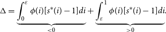 \begin{equation} \Delta =\underset {\lt 0}{\underbrace {\int _{0}^{\varepsilon }\phi (i)[s^{\ast }(i)-1]di}}+\underset {\gt 0}{\underbrace {\int _{\varepsilon }^{1}\phi (i)[s^{\ast }(i)-1]di}}\text {.} \end{equation}
If $\phi (i)=\phi (j)=\phi (\varepsilon )$
for all
$\phi (i)=\phi (j)=\phi (\varepsilon )$
for all $i\in \lbrack 0,\varepsilon ]$
and
$i\in \lbrack 0,\varepsilon ]$
and $j\in \lbrack \varepsilon ,1]$
, then
$j\in \lbrack \varepsilon ,1]$
, then $\Delta =0$
because
$\Delta =0$
because
 \begin{equation} \phi (\varepsilon )\int _{0}^{\varepsilon }[s^{\ast }(i)-1]di+\phi (\varepsilon )\int _{\varepsilon }^{1}[s^{\ast }(i)-1]di=\phi (\varepsilon )\int _{0}^{1}[s^{\ast }(i)-1]di=0\text {.} \end{equation}
Otherwise, $\Delta \lt 0$
because
$\Delta \lt 0$
because $\phi (i)\gt \phi (\varepsilon )\gt \phi (j)$
for any
$\phi (i)\gt \phi (\varepsilon )\gt \phi (j)$
for any $i\in \lbrack 0,\varepsilon )$
and
$i\in \lbrack 0,\varepsilon )$
and $j\in (\varepsilon ,1]$
such that
$j\in (\varepsilon ,1]$
such that
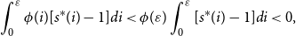 \begin{equation*} \int _{0}^{\varepsilon }\phi (i)[s^{\ast }(i)-1]di\lt \phi (\varepsilon )\int _{0}^{\varepsilon }[s^{\ast }(i)-1]di\lt 0\text {,} \end{equation*}
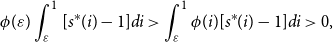 \begin{equation*} \phi (\varepsilon )\int _{\varepsilon }^{1}[s^{\ast }(i)-1]di\gt \int _{\varepsilon }^{1}\phi (i)[s^{\ast }(i)-1]di\gt 0\text {,} \end{equation*}
implying $\Delta \lt \phi (\varepsilon )\int _{0}^{1}[s^{\ast }(i)-1]di=0$
. Therefore, (41) and (42) hold.
$\Delta \lt \phi (\varepsilon )\int _{0}^{1}[s^{\ast }(i)-1]di=0$
. Therefore, (41) and (42) hold.
Appendix B: Alternative innovation specification
In this appendix, we explore the implications of modifying (15) as
 \begin{equation} \frac {\Delta N_{t}}{N_{t}}=\frac {\theta H_{R,t}}{N_{t}}\text {.} \end{equation}
In this case, the steady-state growth rate of $N_{t}$
is determined by the growth rate of
$N_{t}$
is determined by the growth rate of $H_{R,t}$
as
$H_{R,t}$
as
 \begin{equation} \frac {\Delta N_{t}}{N_{t}}=\frac {\Delta H_{R,t}}{H_{R,t}}\text {.} \end{equation}
Recall that the resource constraint on human-capital-embodied labor is given by
 \begin{equation} H_{Y,t}+H_{R,t}=\int _{0}^{1}\left [ 1-e_{t}(i)-\sigma n_{t}(i)\right ] h_{t}(i)L_{t}(i)di\text {,} \end{equation}
where $\{e_{t}(i),n_{t}(i),h_{t}(i)\}$
are constant at the steady state and given by (26)-(28). Therefore, the growth rate of
$\{e_{t}(i),n_{t}(i),h_{t}(i)\}$
are constant at the steady state and given by (26)-(28). Therefore, the growth rate of $H_{R,t}$
is determined by the growth rate of
$H_{R,t}$
is determined by the growth rate of $L_{t}(i)$
given by
$L_{t}(i)$
given by $n^{\ast }$
, which is the same across all households. Therefore, the steady-state growth rate of
$n^{\ast }$
, which is the same across all households. Therefore, the steady-state growth rate of $N_{t}$
is determined by the population growth rate as in Jones (Reference Jones1995, Reference Jones2001) and given by
$N_{t}$
is determined by the population growth rate as in Jones (Reference Jones1995, Reference Jones2001) and given by
 \begin{equation} g^{\ast }=n^{\ast }-1=\frac {\eta }{\sigma (1+\eta +\gamma \delta )}-1\text {,} \end{equation}
which is increasing in fertility preference $\eta$
but decreasing in quality preference
$\eta$
but decreasing in quality preference $\gamma$
, human capital depreciation rate
$\gamma$
, human capital depreciation rate $\delta$
and fertility cost
$\delta$
and fertility cost $\sigma$
. In this case, household heterogeneity in education abilities
$\sigma$
. In this case, household heterogeneity in education abilities $\phi (i)$
does not affect economic growth in the long run. This difference arises because long-run growth is determined by the growth rate of human capital in (B2) in this extended model, rather than the average level of human capital in (15) in the baseline model. Therefore, it becomes an empirical question as to whether the average level of human capital or the growth rate of population is a more relevant determinant of economic growth in the long run.
$\phi (i)$
does not affect economic growth in the long run. This difference arises because long-run growth is determined by the growth rate of human capital in (B2) in this extended model, rather than the average level of human capital in (15) in the baseline model. Therefore, it becomes an empirical question as to whether the average level of human capital or the growth rate of population is a more relevant determinant of economic growth in the long run.
Appendix C: Figure and table
Table 4. Summary statistics
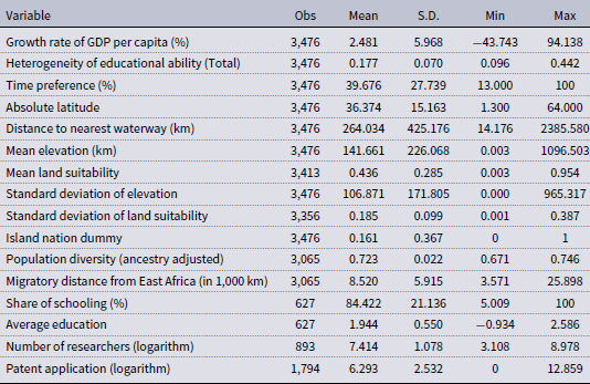
Notes: The heterogeneity of educational ability is calculated using the coefficient of variation of academic scores from the TIMSS database. The heterogeneity of educational years, share of schooling, and average education data are sourced from the Barro-Lee educational attainment dataset. The data on time preference is sourced from Galor and Ozak (Reference Galor and Özak2016) . The land agricultural suitability data is sourced from Michalopoulos (Reference Michalopoulos2012) . Data for absolute latitude, mean elevation, standard deviation in elevation, and an island dummy variable are obtained from the Geographically Based Economic Data (G-ECON) project (Nordhaus, Reference Nordhaus2006). Data for distance to the nearest waterway are from Arbatli et al., (Reference Arbatlı, Ashraf, Galor and Klemp2020) . All other variables are from the Penn World Table.
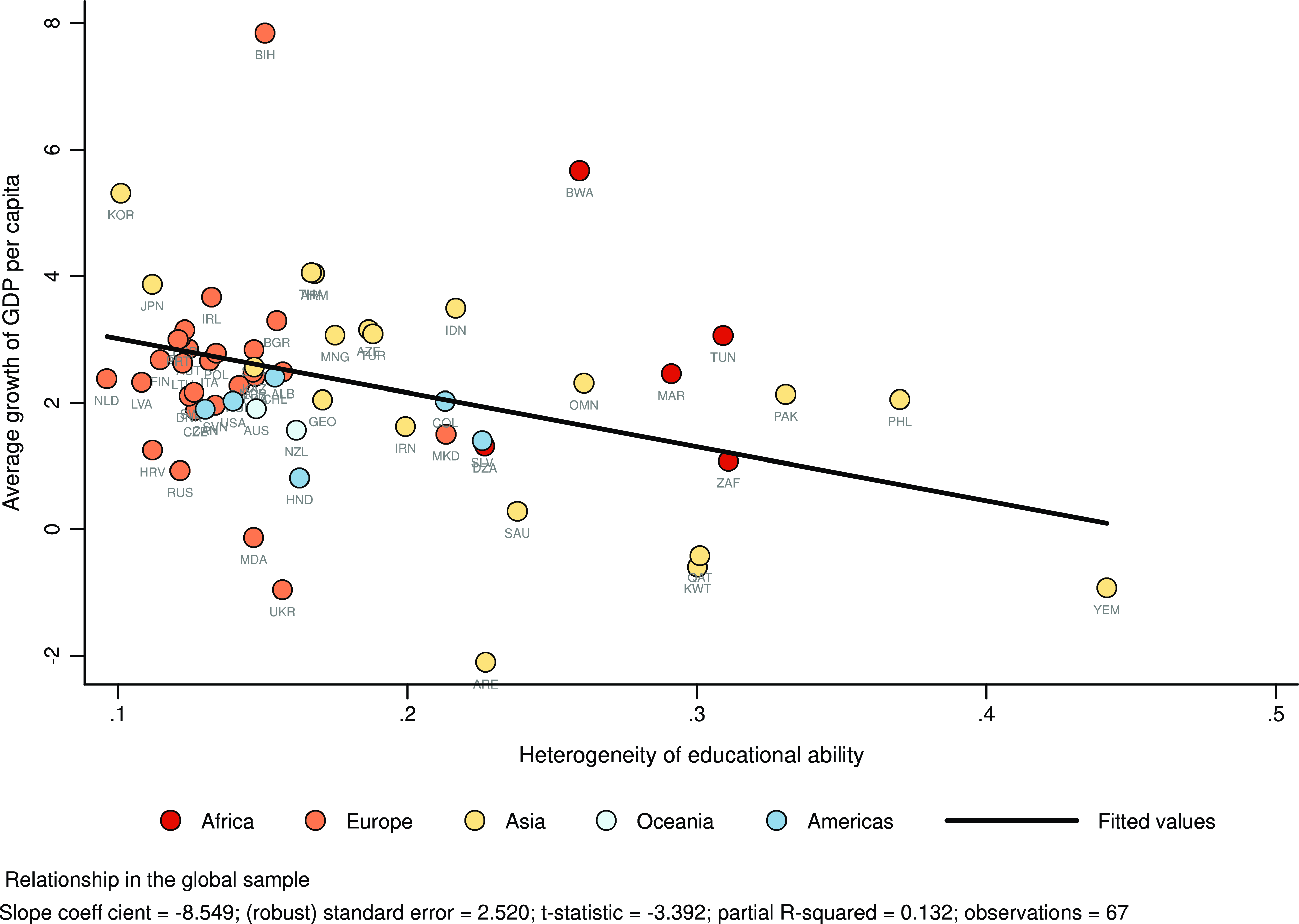
Figure 2. The relationship between heterogeneity in educational ability and economic growth.Notes: This figure illustrates a negative relationship between heterogeneity in educational ability against the country’s average economic growth rate from 1951 to 2017.


 Open access