


1.1 Introduction
This chapter first reviews the linear first-order nonhomogeneous ordinary differential equation. An introduction to statistics and stochastic processes follows. Afterward, this chapter explains the stochastic fluid continuum concept and associated control volume, spatial- and ensemble-representative control volume concepts. It then uses the well-known solute concentration definition as an example to elucidate the volume- and spatial-, ensemble-average, and ergodicity concepts. This chapter provides the basic math and statistics knowledge necessary to comprehend the themes of this book. Besides, this chapter’s homework exercises demonstrate the power of the widely available Microsoft Excel for scientific investigations.
1.2 Linear First-Order Nonhomogeneous Ordinary Differential Equation
Since many chapters and homework assignments use the first-order ordinary differential equation and its solution technique, we will briefly review a simple solution below. A revisit to calculus or an introduction to the differential equation would be helpful.
Consider an ordinary differential equation that has a form:
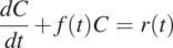 (1.2.1)
where  . It has the general solution:
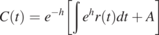 (1.2.2)
where  . Since t is time, the differential equation is called an initial value problem (also called the Cauchy problem). If t is a spatial coordinate, the mathematical problem is called a boundary value problem.
Consider the following ordinary differential equation,
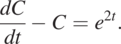 (1.2.3)
Comparing Eq. (1.2.3) with Eq. (1.2.1), we see f(t) = –1, r(t) = e2t, and  in Eq. (1.2.2). Substituting these relationships into Eq. (1.2.2), we have the general solution for the ordinary differential equation,
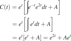 (1.2.4)
in which A can be determined if an initial condition is specified. Otherwise, the problem is not well defined, and many possible solutions exist. As an example, given that C at t = 0 is C0, we find that A = C0 – 1. As a result, a particular solution (unique solution) for this initial condition is
 (1.2.5)
1.2.1 Homework
1. Find the general solutions of the following differential equations
 (1.2.6)
2. Derive the analytical solution to the initial value problem
(1.2.7)3. Evaluate the analytical solution of problem 2 and plot y as a function of t.


1.3 Random Variable
A random, aleatory, or stochastic variable is a quantity whose outcome is unpredictable or unknown, although anything can be viewed as random, as explained later. A mathematical treatment of random variables is the probability, an abstract statement about the likelihood of something happening or being the case.
Suppose we take a bottle of lake water to determine the chloride concentration (C0). While the concentration may have a range of possible values (e.g., 0–1000 ppm), within this range, the exact value is unknown until measured. The concentration C0 thus is conceptualized as a random variable to express our uncertainty about the concentration.
Similarly, repeated measurements of the concentration may yield a distribution of values due to the experimental error. If the measurement is precise, all the values are very close. If not, the values may be widely spread. Such a spread distribution of replicates often assesses the measurement method’s precision or accuracy (an expression of our uncertainty about the measurement). In this case, the C0 is a random variable, expressing our uncertainty about the instrument’s measurement.
The above examples immediately lead to the notion that if the concentration is measured precisely (error-free), the concentration is a deterministic variable, not a random variable. However, this notion may not be necessary. Any precisely known, determined, or measured event is always an outcome of many possible events that could have occurred. For example, the head resulting from flipping a coin is undoubtedly a deterministic outcome since it has happened. On the other hand, it is the outcome of a random variable consisting of two possibilities (head or tail) – a flipping coin experiment. In this sense, everything that happened is the outcome of a random event. This thinking leads to probabilistic science (i.e., statistics).
In statistics, the set of all possible values of C0 of the water sample is a population. This population could be a hypothetical and potentially infinite group of C0 values conceived as a generalization from our knowledge. The likelihood of taking a value from the population is then viewed as chance or probability. Therefore, C0 is a random variable with a probability distribution that describes all the possible values and likelihoods being sampled.
The random variable can be discrete or continuous. A discrete random variable has a specified finite or countable list of values (having a countable range). Typical examples of discrete random variables are the outcome of flipping a coin, throwing dice, or drawing lottery numbers. On the other hand, a continuous random variable has an uncountable list of values. For instance, the porosity of a porous medium, chloride concentration in the water, or any variables in science is a continuous random variable because it has a continuous spectrum of values rather than a countable list of values. Of course, we could approximate the continuous random variable using the discrete random variable by grouping them into a countable list.
In the discrete case, we can determine the probability of a random variable X equal to a given value x (i.e., P(X = x)) from all possible values of X. The set of all the possible values is the probability mass function (PMF). On the other hand, in the continuous random variable case, the probability that X is any particular value x is 0 since the random variable value varies indefinitely. In other words, finding P(X = x) for a continuous random variable X is meaningless. Instead, we find the probability that X falls in some interval (a, b) – we find P(a < X < b) by using a probability density function (PDF).
The porosity of a sandstone formation is an excellent example to elucidate the PDF. Suppose the sandstone formation’s porosity is reported to be 0.3. Intuition tells us that every sample taken from the formation will not be precisely 0.3. For example, randomly selecting a sandstone sample may sometimes find the porosity is 0.27 and others are not. We then ask the probability of a randomly selected sandstone having a porosity value between 0.25 and 0.35. That is to say, if we let X denote a randomly selected sandstone’s porosity, we like to determine P(0.25 < X < 0.35).
Consider that we randomly select 100 core samples from the sandstone, determine their porosity, and create a histogram of the resulting porosity values (Fig. 1.1). This histogram describes the distribution of the number of samples in each range of porosity value (i.e., several bins or classes: 0–0.1, 0.1–0.2, and so on). As indicated in Fig. 1.1, most samples have a value close to 0.3; some are a bit more and some a bit less. This histogram illustrates that arbitrarily taking a core sample will likely have a sample with a porosity of 0.3. Alternatively, if we repeatedly take a sample from the 100 cores, we will get a core with a porosity of 0.3 most of the time. However, a probability of any particular value (e.g., 60%) does not guarantee that we will get 60 core samples with a porosity value of 0.3 after picking a sample over 100 times. This probability is merely an abstract concept that quantifies the chance that some event might happen.
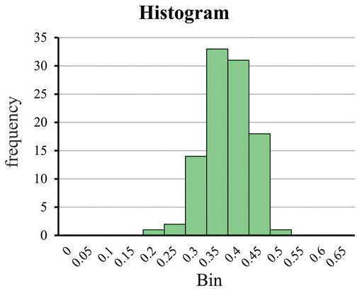
Figure 1.1 The histogram for the porosity value of a sandstone.
Now, we decrease the interval to an infinitesimally small point. X’s probability distribution becomes a curve like in Fig. 1.2, denoted as  and called a probability density function. It shows that the porosity value varies continuously from 0 to 0.7. Notice that the density function could have a value greater than 1, as the histogram could have.
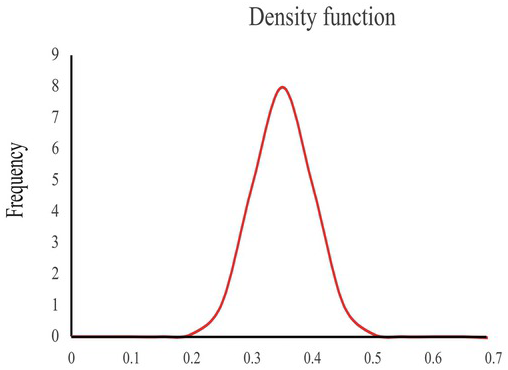
Figure 1.2 An illustration of a density function. The vertical axis is the density, and the horizontal axis is the porosity value.
A density histogram is defined as the area of each rectangle equals the corresponding class’s relative frequency, and the entire histogram’s area equals 1. That suggests that finding the probability that a continuous random variable X falls in some interval of values is finding the area under the curve  bounded by the endpoints of the interval. In this example, the probability of a randomly selected core sample having a porosity value between 0.20 and 0.30 is the area between the two values. A formal definition of the probability density function of a random variable is given below.
Definition. The probability density function (PDF) of a continuous random variable X is an integrable function  satisfying the following:
(1)
, for all x.(2) The area under the curve
is 1, that is:(1.3.1)(3) The probability that x in a bin or class, say,
, is given by the integral of over that interval:(1.3.2)


Again, notice that a probability density function, the number of occurrences of a value x and can be greater than 1, is not a probability.
A widely used PDF is
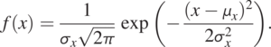 (1.3.3)
This PDF describes a normally distributed random variable X. In the equation, x is the random variable value,  is the mean (i.e., the most likely) value of all x values, and
  is the variance, indicating the likely deviation of x from the mean. Because the random variable has a normal (Gaussian) distribution, it has symmetric and bell-shaped distribution (Fig. 1.3). Thus, the mean and variance fully characterize a random variable with a normal distribution, as indicated by the equation. For this reason, most statistical analyses assume that random variables have a normal distribution, attributing to the mathematical simplicity of Eq. (1.3.3). As PDF is an abstract concept, we never have an infinite number of samples to disapprove of it.
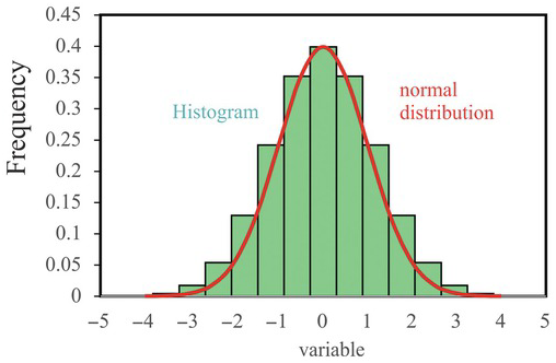
Figure 1.3 A schematic illustration of the histogram and the normal distribution.
Frequency distribution: A frequency distribution is a table or a graph (e.g., a histogram) that displays a summarized grouping of data divided into mutually exclusive classes and the number of occurrences in a class. It becomes a relative frequency distribution if the total number of samples in all classes normalizes the frequency.
Probability distribution: A probability distribution is a mathematical function that produces probabilities of different possible outcomes for an experiment and is an alias for relative frequency distribution.
Cumulative distribution function (CDF): A CDF is a mathematical functional form describing a probability distribution. For example, the cumulative distribution function of a real-valued random variable X, or just distribution function of X, evaluated at x, is the probability that X will take a value less than or equal to x.
Distribution Parameters: The following definitions are theoretical, based on an infinitely large population.
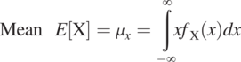 (1.3.4)
where X is the random variable name and x represents the values of the random variable.  denotes the probability density function (PDF) of the random variable, X. E represents the expected value (an average over the infinitely large population). The mean represents the most likely value of the random variable, for example, the average value of the porosity of a sandstone formation.
The variance, a measure of the spread of the distribution, is defined as
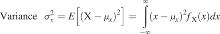 (1.3.5)
The standard deviation is the square root of the variance, the most likely deviation of the random variable value from its mean value. For example, it is often used to construct the upper or lower bound of the sandstone’s porosity value.
While X is used to represent the random variable, and x is the value of the random variable, we use x for both most of the time.
Sample Statistics
Only a finite population and discrete random variables are available in practice. The statistics calculated from these samples are called sample statistics.
Suppose we have samples from I = 1 to N, where N is the total number of samples. The sample mean is calculated as
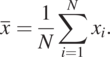 (1.3.6)
The sample variance is given as
 (1.3.7)
Eq. (1.3.7) uses N − 1 to make the estimate unbiased. If N is large, this correction is unnecessary. Besides, how large N is sufficiently large is undetermined since we do not know the population’s size. Likewise, the normal PDF is widely used in many fields because of its mathematical simplicity and insufficient datasets to verify or disapprove the distribution. The following central limit theorem further supports this approach.
The Central Limit Theorem (CLT)
As a statistical premise, CLT states that when independent random variables are lumped together after being properly normalized, their distribution tends toward a normal distribution even if the original variables are not normally distributed. The central limit theorem has several variants. In its typical form, the random variables must be identically distributed. In variants, the convergence of the mean to the normal distribution also occurs for non-identical distributions or for non-independent observations. This theorem is a key in probability theory because it implies that probabilistic and statistical methods that work for normal distributions can apply to many problems involving other types of distributions.
1.4 Stochastic Process or Random Field
Instead of considering a variable, we often simultaneously consider many variables in time or space, leading to the adoption of the stochastic process or field concept. Formally, a stochastic process is a collection of an infinite number of random variables in space or time. Examples are the spatial distribution of porosity or hydraulic conductivity in a geologic formation or the spatial and temporal distribution of a lake’s chemical concentration.
Consider a temporally varying concentration, C(x,t), at a point, x, in space at the time  . If the concentration is not measured, and we guess it, we inevitably consider the concentration a random variable characterized by a probability distribution (PDF). If we guess the C at the time
  , we again consider it a random variable at
  . Guessing the concentration at that location for a period is treating the concentration as a stochastic process over time.
As articulated in the flipping coin experiment, we can conceive any known or deterministic event as a random event. Accordingly, a recorded concentration history at a location that has occurred (or deterministic in conventional thinking) in time and space is a stochastic process or stochastic field. While this concept may be difficult to accept based on the conventional sense, it should become apparent as we apply it to many situations discussed in the book. The fact is that the stochastic process concept is abstract and exists in our imaginary space.
An observed record of concentration history at a location can be considered a stochastic process, consisting of infinite possible concentration-time series over the same period in our imaginary domain. Each possible concentration-time series is a realization (Fig. 1.4). The ensemble is the collection of all possible realizations (analogous to the population for a single random variable). The observed concentration-time series is merely one realization of the ensemble.
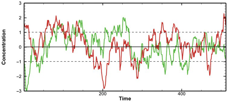
Figure 1.4 Illustration of two possible realizations of a concentration-time stochastic process, assuming jointly normal distribution with mean zero and variance one. The solid black line is the mean, and the two dashed lines are standard deviations.
Determining the possibility (likelihood) of the occurrence of this observed concentration series demands the concept of joint probability density function (or a joint probability distribution, JPD). This JPD is different from the PDF of a random variable since the JPD considers the simultaneous occurrence of some concentration values at different times.
To explain the meaning of the JPD, we consider two random variables (e.g., porosity n and hydraulic conductivity, K) and assume that the logarithm of each of them (log K or log n) has a normal distribution. Fig. 1.5 shows their JPD  . Here X and x denote the variable log K, and its value, respectively. The Y is log n, and y is its value, respectively. The JPD determines the probability of the simultaneous occurrence of porosity and hydraulic conductivity over a range of values. This JPD is different from the probability distribution of each variable individually. The individual probability distribution of X or Y is the marginal probability distribution of the JPD. The marginal probability distribution of X or Y can be determined from their joint probability distribution:
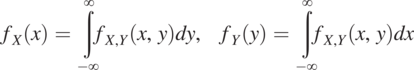 (1.4.1)
The marginal probability is an orthogonal projection of the JPD to the X or Y-axis.

1.4.1 Joint Probability Density Function
A joint probability density function (JPDF) for the stochastic concentration process,  , thus is represented as
  , which satisfies the following properties:
(1)
(1.4.2)

This property states that the JPD must be greater than zero for all concentrations at any time.
(2)
(1.4.3)

The sum of the JPD for all possible concentrations must equal 1.
(3)
(1.4.4)

The probability of occurrence of the concentration of certain intervals is the sum of all JPD over the given intervals.
1.4.2 Ensemble Statistics
Ensemble statistics assume that the ensemble (i.e., all possible realizations) is known. If the JPD of the process is Gaussian, the first and second moments are sufficient to characterize the stochastic process. Otherwise, this is the best we can do.
Mean (1st moment) is defined as
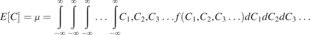 (1.4.5)
The expectation value, E, is carried out over the entire ensemble. The mean,  , thus is the average (the most likely) concentration value over the ensemble.
Covariance or Covariance function (2nd moment) is defined as
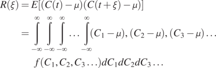 (1.4.6)
In Eq. (1.4.6),  is the separation time between two concentrations (random variables) at two different times. As a result, the covariance measures the temporal relationship between the concentrations at a given time and other times, characterizing the joint probability distribution of a stochastic process. If the separation time is zero, the covariance collapses to the variance of the process. That is,
 (1.4.7)
The variance is always positive, and covariance is symmetric and could have negative values at some separation time, for instance, a periodic time series (see Fig. 1.10).
Autocorrelation or Autocorrelation function is the covariance normalized by the variance:
 (1.4.8)
It has the following properties:
1. The autocorrelation function is always symmetric.
2.
and it is always a real number.3.
.


The autocorrelation function is a statistical measure of the similarity of the concentration-time series offset by a given separation time. It often is used to detect the periodicity of the time series.
1.4.3 Stationary and Nonstationary Processes
A stationary process is a stochastic process where the JPDs or statistical properties do not vary with temporal or spatial locations. This concept is analogous to the spatial homogeneity of geologic media’s hydraulic properties or the spatial representative elementary volume concept (spatial REV, Yeh et al., Reference Yeh, Khaleel and Carroll2015, or Section 1.5). A second-order stationary process requires only the first and second moments of the JPD to be stationary. For a Gaussian JPDF, a second-order stationary process implies stationary. If a process does not meet this requirement, it is a nonstationary process. For instance, the time series, which has a large-scale trend (e.g., seasonal or annual trends), is nonstationary. In reality, natural processes are nonstationary since they have multi-scale variability. Nonetheless, they can always be treated as stationary since the large-scale trend can always be conceptualized as a stochastic process (an abstract concept).
Suppose one treats a nonstationary process as a stationary process. One implicitly includes the large-scale trend as the stochastic process. As such, the variance of this “stationary” process is large since it includes the variability of the large-scale trend. If the large-scale trend is known and characterized, it can be removed as a deterministic feature. The residual variable (after removing the trend) can then be stationary if the residual statistics are invariant. In this case, the variance of the residual should be smaller than the original.
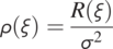
The above stochastic analysis assumes that the JPD is jointly Gaussian, like all statistical analyses. Therefore, a jointly Gaussian stochastic process is fully characterized if the mean and the autocovariance function are specified. An illustration of JPD of a Gaussian stochastic process is formidable. Nevertheless, we show in Fig. 1.6 a bivariate JPD with different correlations (covariances). As shown in Fig. 1.6, if two random variables are uncorrelated, their JPD is concentric bell-shaped. An increase in the correlation between the two variables squeezes the JPD’s symmetric bell shape to an elliptic one. This correlation effect is further explained in Fig. 1.9.
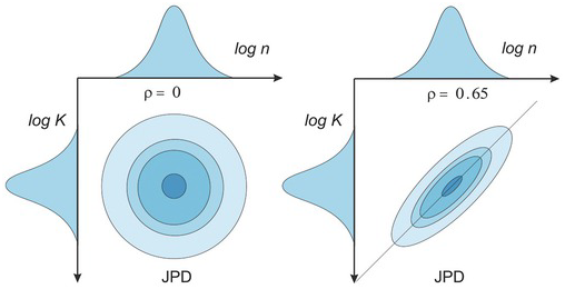
Figure 1.6 Effects of correlation on bivariate (log K and log n) JPD. ρ is the correlation between the two random variables.
1.4.4 Sample Statistics
As already discussed, the stochastic concept and theories are built upon the ensemble. In reality, we, however, can only observe one realization. Owing to this fact, we must adopt the ergodicity assumption as we apply stochastic theories to real-world problems. The ergodicity states that the statistics from the time series we observed represent the ensemble statistics as long as the series is sufficiently long. Of course, how long is sufficiently long is a question. “Up to one’s judgment” is the answer since we never know the ensemble, and no one can discredit your assessment. In other words, ergodicity is our working hypothesis – the best we can do.
Furthermore, our observed time series always has a finite length, and the samples and records are not continuous but discrete. We, therefore, developed methods to calculate the sample statistics as follows:
Consider the case in which we take N concentration measurements,  , at a regular time interval
  at a lake’s location. The mean of the concentration-time series is
 (1.4.9)
While this formula is identical to the sample mean of a random variable (Eq. 1.3.6), this concentration-time series is a stochastic process. Also, Eq. (1.4.9) is a temporal averaging, not ensemble averaging, implicitly invoking the ergodicity assumption.
To calculate the temporal relationship between the concentration value at  and at other times, we use the sample covariance function:
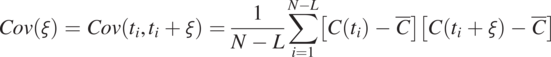 (1.4.10)
In Eq. (1.4.10),  (separation time);
  is the sampling time interval; L is the number of intervals, ranging from 1 to N − 1. Fig. 1.7 illustrates the operation of this equation. When L = 1, Eq. (1.4.10) calculates the sum of the product of the N − 1 pairs of concentration perturbations (concentration minus its mean) separated by one
  , and the resultant is then divided by N − 1. As L = 2, it repeats the calculation for N − 2 pairs separated by twos. This procedure is repeated until L = N − 1, or only one pair of concentrations is left.
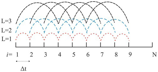
Figure 1.7 An illustration of the autocovariance algorithm (Eq. 1.4.10).
As L = 0, the covariance is the sum of the product of  and itself at all measurement times and divided by N. It becomes the variance, denoted as S2.
 (1.4.11)
Eq. (1.4.10), the sample covariance function, examines the relationship between pairs of concentration data separated at different numbers of  s by increasing the L value. Notice that increasing L decreases the number of pairs for the product operation, reflected by N − L’s value. For example, when L = N − 1, the formula has only one pair of concentrations (i.e.,
  and
and  for calculating the covariance. As L becomes large, the number of pairs for evaluating the covariance becomes small. The estimated covariance is thus not representative the time series’s actual covariance and is often discarded.
Notice that some prefer to use N − L − 1 instead of N − L for the denominator in Eq. (1.4.10) for unbiased estimates. However, statistics are merely a bulk description of a process, and such a theoretically rigorous treatment may not be necessary for a practical purpose.
Graphical interpretation of Eq. (1.4.10) is given in Fig. 1.8, where the solid black line denotes the observed time series of the concentration, and the red dashed line represents the observed series after being shifted by a separation time  . Eq. (1.4.10) sums up the products of the pairs of C values of the solid black and dashed red lines at every t inside the overlapped yellow area. It then divides the sum by the total number of pairs within the area to obtain the covariance at a given separation time interval
  . Subsequently, the two series are shifted by another
  , and the above procedure is repeated till the overlapping area is exhausted.
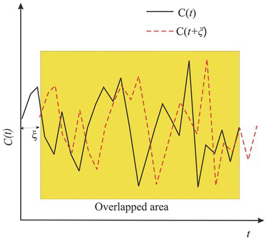
Figure 1.8 An illustration of the physical meaning of the autocovariance function.
Eq. (1.4.12) defines the sample autocorrelation function
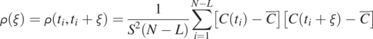 (1.4.12)
which is simply the covariance (Eq. 1.4.10) normalized by the variance (Eq. 1.4.1). After the normalization, the maximum autocorrelation is 1, and the range of the correlation is bounded by −1 and +1. Eq. (1.4.12) can be implemented in Microsoft Excel (see homework 1.2).
Scatter plots in Fig. 1.9 explain the physical meaning of the autocorrelation function. Instead of summing the products of different pairs of time-series data using Eq. (1.4.12), we plot each pair of data series in the overlapped area with different shifts (separation times  , and 30) on a X−Y plot and then carry out a correlation analysis (Eq. 1.4.12), as illustrated in Fig. 1.9a, b, c, d, e, and f, respectively. Each plot shows the correlation value
  between the time series and that after a shift. When the shift is zero, the data pairs from the solid black and dashed red lines in Fig. 1.8 overlap on the 45-degree (1:1) red line, and the correlation value is one, indicating that these data pairs are perfectly correlated (identical). As the shift becomes large, the data pairs start scattering around the 1:1 line, and the correlation value drops below 1, indicating that the shifted dashed red line is dissimilar to the solid black line in Fig. 1.8. As the shift becomes large, the dissmilarity becomes significant, and the correlation drops further.
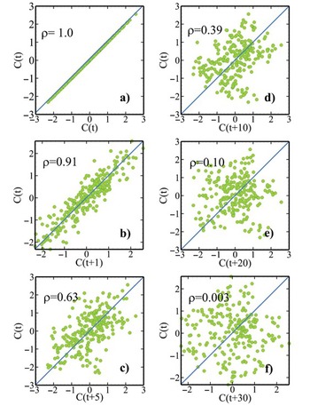
Figure 1.9 Scatter plots to elucidate the physical meaning of autocovariance function calculation. They show how the similarity between the original concentration time-series and those shifted with different time intervals.
These scatter plots manifest that an autocorrelation analysis compares the time series at different separation times for their similarity based on the linear statistical correlation analysis. Accordingly, autocorrelation analysis is a valuable tool for finding the time the recurrence of similar events in a time series (e.g., diurnal, seasonal, or annual variation in precipitation, temperature, or flood events of certain magnitudes).
Figure 1.10a shows a sinusoidal time series infested with white noises (i.e., uncorrelated random noise at a scale smaller than the sampling time interval). This series is nonstationary or has multi-scale variability. Its autocorrelation function is plotted in Fig. 1.10b. The autocorrelation function reveals that the peaks and troughs of the time series reoccur at a period of 60 and the effect of non-periodic white noise at the origin (also see stochastic representation in Chapter 9).
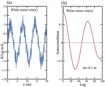
Figure 1.10 A periodic sine concentration time series corrupted with white noise is shown in (a). The time series autocorrelation function (b) indicates the periodicity of the sine function and noise. The sudden drop of the autocorrelation value at the origin reflects that the noise is non-periodic.
Likewise, Fig. 1.11 displays the sample autocorrelation functions of the two realizations of stochastic time series in Fig. 1.4, which does not have a noticeable large-scale periodic component as in Fig. 1.10a. First, the two realizations’ autocorrelation functions decay as the separation time increases, but they are not identical. The difference manifests the non-ergodic issue of a single realization of a stochastic process of a short record. Second, the autocorrelations drop from 1 to 0 as the separation time increases beyond the separation time around 50, indicating that the pairs of concentration data, separated by the separation time greater than 50, are unrelated (or statistical independent). Statistical independence means that one value’s occurrence does not affect the other’s probability.

Further, the autocorrelation at the separation time greater than 50 becomes negative. A negative correlation value means that the time series are correlated negatively at this separation time – the series are similar but behave oppositely. Notice that the autocorrelations fluctuate at large separation times due to the small number of pairs available for the analysis. Thus, the autocorrelation values at these separation times are deemed unrepresentative.
This section introduces the basic concepts of the stochastic process, which will be utilized throughout this book to explain observations and theories of flow and solute transport in the environment. While the time series are used to convey the stochastic concept, the concept holds for spatial series, where the variable varies in space (to be discussed in Chapter 9).
In summary, a stochastic process comprises many possible realizations in our imaginary domain with a given joint probability density function. The distribution is generally considered a joint normal or Gaussian distribution (although not limited to). For this reason, a stochastic process can be described by its mean and covariance function. If the process’s distribution is not Gaussian, the mean and covariance description is merely approximation – the best we can do and a working hypothesis for our scientific analysis.
1.4.5 Homework
The homework’s exercises below intend to demonstrate the power of widely available Microsoft Excel for scientific and engineering applications and enhance understanding of stochastic processes and autocorrelation functions.
(1.1) Use Microsoft Excel to create 80 cells (time steps). Assign a constant temperature value 1 for the first 10 cells and a value of −1 to the next ten cells. Repeat this pattern until the end of the 80 cells (Fig. 1.12). Use Eq. (1.4.12). This equation can be implemented in Excel using the following formula.
=SUMPRODUCT(OFFSET(data,0,0,n-lag,1)
-AVERAGE(data),OFFSET(data,lag,0,n-lag,1)-AVERAGE(data))/DEVSQ(data). (A1)
Data in the above formula is the entire data set, n is the total number of data points (80), and lag is the L in the equation. The lag ranges from 0 to 20. Calculate the autocorrelation function of this series, following the instruction below:
First, create a column for the data. Select “formulas” in the Excel manual, then select “Name Management” and define “data” as the name of the corresponding cell locations of all data in the column.
Next, create a new column with name “lag” and assign 0, 1, through 20 to this new column. Use the name management to define the lag with the cell location of the first lag.
Create another new column with the name “ACF”. In the first cell below the name ACF, enter the formula in Eq. (A1).
Drag this cell down to reach lag = 20, creating the autocorrelation values for ACF column.
Plot the temperature data set vs time and the autocorrelation function vs. lag.
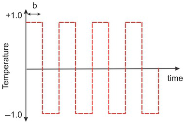
Figure 1.12 The graph shows the temperature variation as a function of time.
Determine the lag where the correlation value is close to zero. Is this lag close to the time step where the C value is constant? What does this result imply? Why does the correlation value drop at large time lags? (Hint: finite length)
(1.2) Generate autocorrelated random time series using Excel.
This homework exercise shows a simple Excel approach to generate an autocorrelated random time series, derive the sample autocorrelation function (ACF), and fit an exponential ACF to the sample ACF for estimating the correlation scale (lambda). Follow the steps below.
(1) Use “RAND()” function in Excel to generate a column of 500 random numbers (ranging from 0 to 1) vs row numbers in column A. Select the 500 random numbers and press CTRL C, then Shift F10, and then V to freeze the random number just generated. The series of the random number is a realization of an uncorrelated random field – Column A.
(2) Plot this realization of the random field and its histogram. Determine the mean and variance.
(3) Calculate and plot the autocorrelation function (ACF) vs. lag of Column A using the procedure in Problem 1. The ACF should drop from 1 rapidly after the first lag, indicating an uncorrelated random field.
(4) In the first cell of another column (e.g., Column B, cell B1), generate a random number using = RAND(). Then, set the next cell as “= B1”) and drag this cell to the following eight cells. This step creates 10 cells with the random number, the same as the first one. Select the generated ten cells with the same random number and drag it down to yield 500 numbers, partitioned into 50 segments. Each segment has a different random value. Freeze this column, and this column of data will be Column B.
(5) Create another column (Column C), being the sum of Columns A and B, yielding a realization of an autocorrelated random field. Afterward, carry out the autocorrelation analysis of this realization, using the procedure in Problem 1.1 to obtain a sample ACF. Determine mean and variance and show the histogram. Plot the random fields of Columns A and C, and the sample ACF vs. lag of Columns C. Compare the ACFs of the two to see the differences between Columns A and C. Verify that this random field Column C correlates over more lags than in Column A.
Fitting an Exponential ACF Model to the Estimated ACF
(6) Set a cell as “lambda” (correlation scale) and assign a numerical value to the next cell. Then define lambda (correlation scale) with the cell using the name manager as in problem 1.
(7) Create a new column with a length of the lag (1–20). Enter “= EXP(-lag/lambda)” at the first cell and drag it along the column to lag = 20, yielding the predicted theoretical ACF at each lag based on the exponential function with the given lambda value.
(8) Set up another column with the name “Error^2”, which is the square of the difference between the sample ACF from the random field with the predicted theoretical ACF. Below the end of this column, create a cell, “sum error^2”, as the sum of all cells of the Error^2 column.
A nonlinear regression solve must be used to find the optimal lambda value that best fits the exponential ACF to the sample ACF. We need to use Solver Add-in in Excel. This nonlinear regression tool is extremely helpful for the analyses and homework in the book.
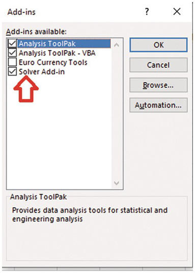
Install Solver Add-In (If it is not installed).
Press “File” tab and then select “option”.
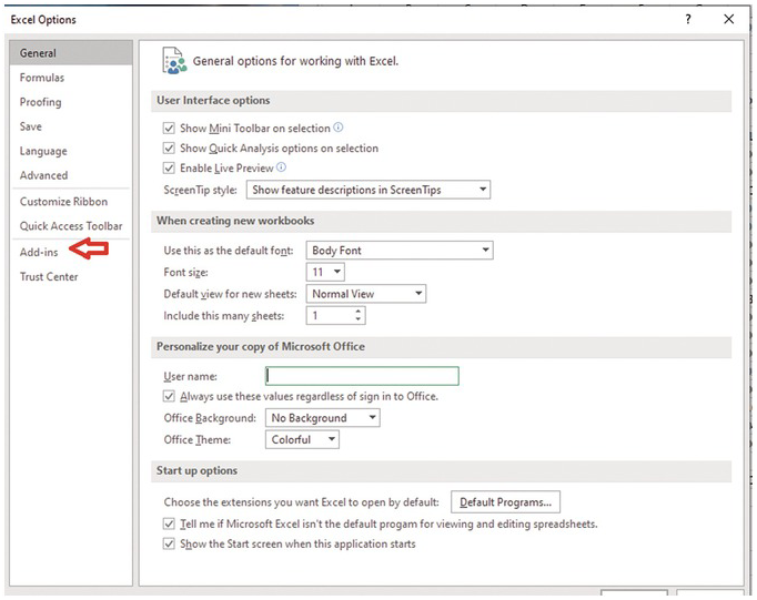
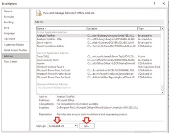
Press go. Then select solver add-in, and then press OK.
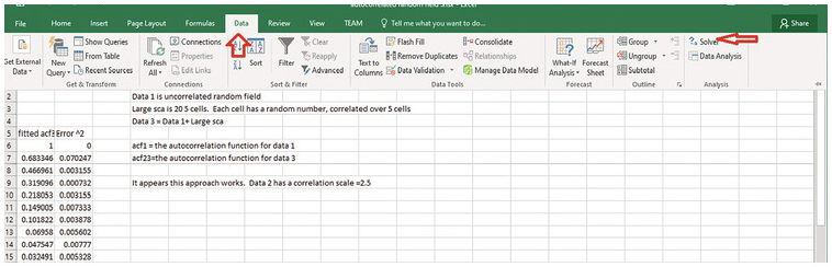
Back to excel sheet and select data and solver should appear.
Click Solver. (1) define the objective, which is the cell numbere of the sum of error^2. (2) Then select Min (minimizing the sum of error^2). (3) Enter lambda (or the cell location of the paramter to be adjusted). (4) Select GRG Nonlinear solving method.
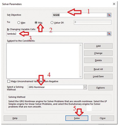
(5) Press solve. Excel will automatically change the lambda value to derive the minimal sum of error^2. Meanwhile, the column of the predicted theoretical ACF will be updated to be the best-fit ACF.
Plot the sample and the best-fit theoretical ACF. Discuss the relationship between the correlation scale (the lambda value) and the number of cells with the constant value. Is it close to 1/2 of the number of cells?
(1.3) Explain why the autocorrelation is one when the L is zero, but the covariance is the highest and decreases as the L becomes large, as the correlation becomes small?
1.5 Stochastic Fluid-Scale Continuum
After the basic concepts of stochastic processes, we are ready to illustrate their importance in the classical “deterministic” fluid properties in the fluid-scale continuum.
1.5.1 Fluid Continuum and Control Volume
Like any scientific study of natural phenomena, fluid mechanics makes underlying assumptions about the materials under investigation. For example, the fluid properties in fluid mechanics refer to the properties of a point in the fluid. However, suppose we randomly pick a point (an infinitesimally small volume) in a fluid. Due to the fluid matter’s discrete nature, that point might be within an atomic particle or in the space between atomic particles. Therefore, the fluid “properties” associated with a point in fluid mechanics would depend upon the measurement point’s location. This point concept creates a discontinuous distribution of properties in space for the substance, prohibiting calculus and differential equations built on smoothness and continuity. To avoid this problem, scientists and engineers employ the continuum assumption. In other words, they use the “volume-average” concept to idealize the fluid macroscopically continuous throughout its entirety; the molecules are being “smeared” or “averaged” to eliminate spaces between atomic particles and molecules. Similarly, the volume-averaged velocity in fluid mechanics conceals continuous collisions between molecules and omits molecular-scale velocities in fluid mechanics.
Indoctrinated by the continuum assumption, the fluid’s physical or chemical attribute at a point in fluid mechanics’ mathematics is the property in a small volume of the actual space. For example, a solute concentration is the mass of solute molecules (M) per volume of the solution  :
:
 (1.5.1)
This volume must be large enough to contain many molecules and is called a control volume (CV). This CV is our “sample volume” or “sample scale” from which we measure or define the fluid’s attributes (such as force, temperature, pressure, energy, velocity, and other variables of interest in fluid mechanics or properties). Such a volume-average attribute ignores the distribution of molecules. For instance, a concentration informs us of the total solute mass, not the solute’s spatial distribution in the volume.
The control volume could also be a volume over which we conceptualize the fluid’s states, conduct mass or energy balance calculations, or formulate a law (e.g., Darcy’s or Fick’s law). Therefore, it can be our model volume or model scale.
1.5.2 Spatial Average, Ensemble Average, and Ergodicity
Suppose we define a volume-averaged fluid property in a volume of 1 m3 fluid, using a small CV (0.01 m3) at various fluid locations, and find the property is translationally (or spatially) invariant. This CV is then the property’s representative elementary volume (REV). The word representative implies that the fluid properties observed in this volume (0.01 m3) are identical to those observed in other fluid locations (1 m3). On the other hand, the word “elementary” means that the volume (0.01 m3) is smaller than the entire fluid body and is an element of the entire fluid (1 m3).
If this REV exists, the fluid is considered homogeneous regarding the property defined over this CV. Otherwise, the fluid is heterogeneous. Notice that the property defined over CVs smaller than the REV may still be heterogeneous – varying in space, implying homogeneity or heterogeneity definition is scale-dependent.
The REV concept is analogous to the size of the moving averaging window in signal processing. Suppose the window size (smaller than the entire record of signals) encompasses enough spatially varying signals to capture the representative characteristics of the entire signal record. This size of the window is a REV. Because this classical REV concept rests upon spatial invariance, it is most appropriately called the spatial REV, which is different from the ensemble REV to be explained next.
The following concentration examples explain the differences in spatial average and ensemble average concepts. Suppose we define the concentration at every point in a solution of 1m3 by overlapping a small CV of 0.01 m3 to obtain a continuous concentration distribution  . The x is a location vector, x or (x, y) or (x, y, z) for one, two, or three-dimensional space.
If  is invariant in x, the solution is well mixed at this CV, and this CV of 0.01 m3 is the concentration spatial REV. Otherwise, the solution is poorly mixed, and this CV is not a spatial REV. Nonetheless, albeit
  varies in x, one may treat the solution of 1m3 well mixed by defining the concentration as the total mass normalized by the total volume (1 m3), ignoring the spatially varying concentration defined at the CV of 0.01 m3. This well-mixed proposition arises from our lack of interest in the detailed solute concentration spatial distribution within this volume (1 m3). This argument leads to the following discussion of CV and REV concepts for the concentration of a solute.
Consider a discrete solute molecule distribution everywhere in a one-dimensional solution domain, as illustrated in Fig. 1.13a. Suppose we adopt a small CV to define the solute concentration and continuously overlap the CV at every point along this line, yielding a continuously but spatially varying concentration distribution, i.e., a poorly mixed solution (Fig. 1.13b). This distribution is characterized by a spatial mean and a spatial variance, representing the most likely concentration and the concentration’s variability above the mean. The mean and variance calculated from the observed concentrations over the domain are spatial statistics.
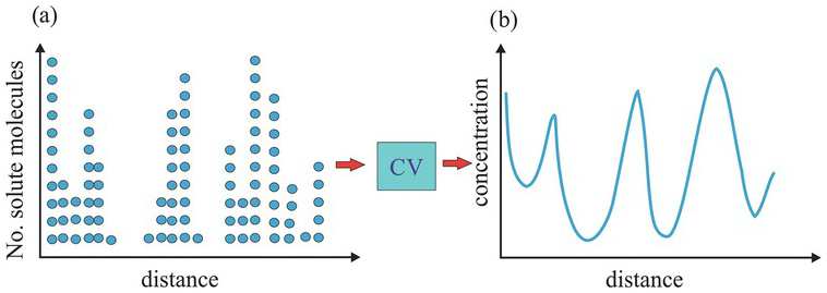
Figure 1.13 Effects of smoothing by a CV. A volume-averaging procedure over a CV converts a discrete and erratic solute spatial distribution into a continuous concentration distribution. The blue circles denote molecules.
By enlarging the CV’s size yet smaller than the entire domain, we may obtain a constant concentration everywhere (equivalent to the spatial mean). These CVs are spatial REVs, as illustrated in Fig. 1.14b, and the solute defined over these sizes’ CV is considered well-mixed.
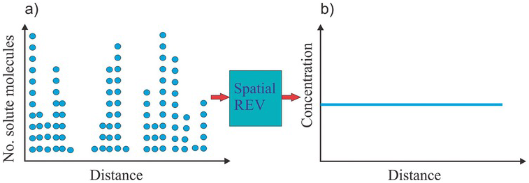
Figure 1.14 If a CV is sufficiently large and its average concentration is translationally constant, the CV is called a spatial REV and the solute is considered well mixed.
There are situations where the concentration field,  , remains varying in space even if the size of the CV is increased (e.g., Figs. 1.15 a and b): the
  always exhibits a spatial trend (a large-scale variation). Despite this trend, one can employ the entire domain as a fixed CV to determine a volume-averaged concentration over the entire domain and treat the solution well-mixed (Fig. 1.16). This CV is fixed in space and is not spatially translational, as are those used to define
  . Such a well-mixed solution proposition based on the entire domain implies a spatial REV since the volume-averaged concentration over this fixed large CV is the mean concentration of the entire domain, satisfying the representativeness requirement of a REV. However, such a large CV is not the solution’s elementary volume; therefore, it is not a spatial REV. The ensemble concept discussed next resolves this paradox.
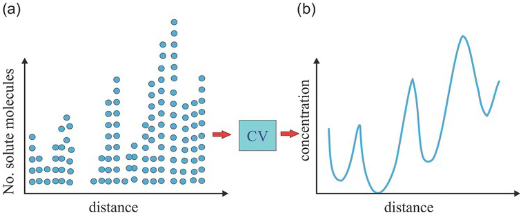
Figure 1.15 (a) The solute particle distribution has a higher number of particles toward the right. (b) The blue line represents the spatial distribution of concentration (% of solute particles over a small CV). The distribution is a continuously varying concentration field with an increasing trend toward the right. The solution is poorly mixed.
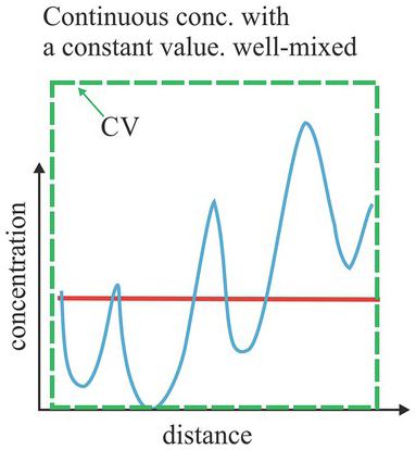
Figure 1.16 The blue line represents the concentration along a line, which exhibits variation and an increasing trend to the right. The red line is the volume-average concentration over a CV, covering the entire solution.
The ensemble concept envisages that the observed spatially varying concentration field with a trend or not in the domain is merely a possible spatial distribution (realization) of many possible ones (ensemble), characterized by a JPD. In other words, an infinite number of CVs of the size as large as the entire domain exists, with its own spatially varying concentration field but the same spatial mean and variance, describing the concentration field’s spatial variability in each CV (see Fig. 1.17). Such mean and variance are the ensemble mean and variance.
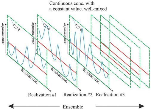
Figure 1.17 The volume-averaged constant concentration of a solution field can be viewed as the mean concentration of many possible solute concentration distributions over CVs of the same size in the ensemble space. In order to restrict the size of the ensemble, we constrain it by requiring that all the concentration realizations have the same spatial mean and variance.
This concentration of the CV fixed in space as large as the entire domain thus possesses the same mean and variance as other realizations and is a realization of the ensemble. It satisfies the representativeness and elementary volume requirements of a REV. As a result, this large CV fixed in space qualifies as an ensemble REV (in our imaginary space), albeit it is not the spatial REV. Following this argument, any size CV is an ensemble REV at a point in space. That is to say, a volume-averaged concentration at a point is an ensemble-averaged concentration at that point. Ultimately, the ensemble REV is a more general definition of REV than the classic definition since it includes the spatial REV.
Once the ensemble REV is accepted, acquiring the JPD of the ensemble becomes a question since all the realizations in the ensemble are unknown. The “Ergodicity” assumption address this question, which states that the spatial statistics from our observations (one realization) are equivalent to the statistics of the ensemble. In plain English, we see one, and we see them all. As is, it may be counterintuitive because the ensemble is unknown. Nevertheless, we accept it as a working hypothesis – the best we can do.
At this point, readers may wonder about the need for these statistical concepts at the beginning of this book. This need arises because multi-scale heterogeneity exists in nature, they are unknown, and all our theories, laws, and observations inherently embrace the ensemble-average concept. For instance, a measured property may be deterministic, but it is an ensemble-averaged quantity – ignoring details within the volume. As we investigate the details within the volume, we find that the details are inherently stochastic (unknown). This stochastic nature of the property or process has often been ignored because it is beyond our observation scale and interest. As we extrapolate these theories and laws to field-scale problems much larger than our observation scales, these stochastic concepts become relevant to comprehending the stochastic nature of the classical theories for solute transport.
1.5.3 Flux Averages
Besides the volume and ensemble averages, flux averages are used to investigate solute transports in the environment, as discussed below (Fig. 1.18).
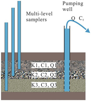
Figure 1.18 A schematic illustration of volume and flux averaged concentrations.
The classic solute transport analysis (e.g., Kreft and Zuber, Reference Kreft and Zuber1978; Parker and Van Genuchten, Reference Parker and Van Genuchten1984) has recognized two types of averaged concentrations.
1. Volume-Averaged (or resident) Concentration: the mass of a solute per unit volume
(1.5.2)

A typical example of volume-averaged concentration is illustrated in Fig. 1.17. If three point sampling boreholes (left-hand side of the figure) tap into dolomite, gravel, and sand layers of an aquifer, concentrations of some chemical at the three depths are sampled (namely,  ,
,  , and
, and  ). The volume-averaged concentration is
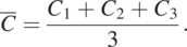 (1.5.3)
Such a volume-averaged approach is likely inappropriate in many applications. For example, as illustrated in the figure’s right-hand side, a pumping well is fully screened over the entire aquifer. The concentration sampled from the discharge from the well is average. However, this average weighs heavily on the concentration from the gravel layer, which has the highest discharge to the total well discharge Q. As a result, a flux-averaged concentration is most appropriate to represent the sample concentration.
2. Flux-averaged (flux) concentration
:(1.5.4)


 ,
,  , and
, and  are discharges to the well from layers 1, 2, and 3. Likewise, the concentrations in layers 1, 2, and 3 are denoted by
 , and
, and  . The right-hand of Eq. (1.5.4) is a continuous form of the flux-averaged concentration. In the equation,
  and
and  are the concentration and specific discharge at any point in the aquifer. A denotes the total surface area of the screening interval.
Kreft and Zuber (Reference Kreft and Zuber1978) and Parker and Van Genuchten (Reference Parker and Van Genuchten1984) pointed out that the resident or flux concentration could lead to different analytical solutions for the advection–diffusion equation. Nevertheless, the importance of the differences would depend on our scales of observation, interest, and model. Therefore, we will adopt the residence concentration throughout the rest of this book.
Units of Concentration: The commonly used unit for concentration is mass per volume (mg/liter). However, it is convenient to express the solute concentration in mass per mass unit as described below for many situations where fluid density varies in time and space (e.g., compressible fluids).
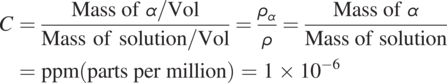
For water at room temperature, 1 liter (l) of water is about 106 mg. Therefore  (part per million). This allows the conversion of volume-averaged concentration to the mass per mass basis concentration definition.
1.6 Summary
A random variable has a probability distribution characterized by a mean and variance.
A stochastic process is a collection of many random variables. It has a joint probability distribution, characterized by a mean and autocovariance function, which quantifies the statistical relationship between the random variables.
If the property in a CV at every point is known, spatial or volume average and autocovariance can be defined. Otherwise, they are strictly ensemble statistics. The spatial and ensemble statistics are equivalent if ergodicity is met or the number of samples is sufficiently large.
All properties in the fluid continuum are ensemble means over a given CV.
The ensemble REV concept is more general than the classical spatial REV since it applies to spatially variable properties or processes with a trend or not.


