


1 Introduction
It is over a century since William Bray [Reference Bray5] became the first researcher to suggest that oscillating chemical reactions might be possible within a homogeneous solution; he reported on what is now known as the Bray–Liebhafsky reaction. In the following few years Bray’s results were treated with some scepticism [Reference Noyes and Field24] as many thought that his findings must be unphysical. Conventional wisdom at the time was that chemical reactions should tend towards an equilibrium state [Reference Zhabotinsky35, Reference Zhabotinsky36]. Indeed, it was only after considerable further work on this class of reactions that it was eventually conceded that chemical oscillations not only are theoretically feasible but also can occur in practice [Reference Winfree32]. It is likely that one obstacle along the path to a general acceptance of the ideas forwarded in [Reference Bray5] is due to an inherent difficulty in seeing the oscillations in the laboratory. Bray suggested that the concentrations of iodine and iodate play pivotal roles in the mechanisms that are operative but, unfortunately, the changes caused by these oscillations in concentration are difficult to observe visually. By way of contrast, more contemporary oscillating chemical reactions, such as the Belousov–Zhabotinsky [Reference Zhabotinsky35] and Briggs–Rauscher reactions [Reference Briggs and Rauscher6], are much easier to observe as they are characterized by vivid colour changes. Oscillations in the Bray–Liebhafsky reaction can only be verified by invoking quantitative methods such as UV-visible spectrophotometry [Reference Maksimović, Tos˘ović and Pagnacco22] or electrochemistry [Reference Ševčík, Kissimonová and Adamcikova27].
Following the pioneering study [Reference Bray5] there have been numerous investigations into other chemical oscillators. Perhaps the most famous among these is the Belousov–Zhabotinsky process [Reference Tyson30]; extensive studies, such as those in [Reference Becker and Field2, Reference Forbes14] have examined the temporal oscillations and spatial patterns that may form during this reaction. Subsequent experiments have confirmed many of these theoretical predictions [Reference Belmonte, Qi and Flesselles3]. On the other hand, there has been a relative dearth of analysis of the Bray–Liebhafsky reaction and, in particular, we are not aware of any studies that inquire as to the feasibility of spatial patterning. It is this issue that we intend to address in the work described below.
The mechanism that underpins the Bray–Liebhafsky reaction is notably complicated. While the full details of the process are still not fully understood, the basic idea is that the oscillations arise from the autocatalysis of iodate and iodine in the presence of hydrogen peroxide [Reference Sharma and Noyes28]. The reduction–oxidation equations that model these autocatalytic reactions are
 $$ \begin{align*} &5\mathrm{H}_2\mathrm{O}_2+\mathrm{I}_2 \longrightarrow2\mathrm{I}\mathrm{O}_3^-+2\mathrm{H}^++4\mathrm{H}_2\mathrm{O}, \\ &5\mathrm{H}_2\mathrm{O}_2+2\mathrm{I}\mathrm{O}_3^-+2\mathrm{H}^+\longrightarrow \mathrm{I}_2+5\mathrm{O}_2+6\mathrm{H}_2\mathrm{O}, \end{align*} $$
which, when combined, give the net reaction
 $$ \begin{align*} 2\mathrm{H}_2\mathrm{O}_2 \longrightarrow 2\mathrm{H}_2\mathrm{O} + \mathrm{O}_2. \end{align*} $$
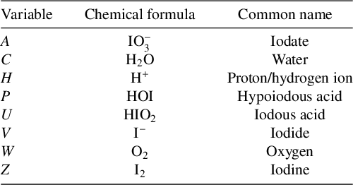
The various chemicals involved here are identified in Table 1. Owing to the autocatalytic nature of this reaction, oscillations in the concentrations of iodine ( $\mathrm {I}_2$
) will occur until all of the hydrogen peroxide (
$\mathrm {I}_2$
) will occur until all of the hydrogen peroxide ( $\mathrm {H}_2\mathrm {O}_2$
) has been consumed. Therefore if hydrogen peroxide is added in a great excess this reaction can continue almost indefinitely. Practical experiments of the reaction can easily extend to several days or even weeks, although the exact duration is also a function of the temperature [Reference Bray5].
$\mathrm {H}_2\mathrm {O}_2$
) has been consumed. Therefore if hydrogen peroxide is added in a great excess this reaction can continue almost indefinitely. Practical experiments of the reaction can easily extend to several days or even weeks, although the exact duration is also a function of the temperature [Reference Bray5].
Table 1 Identification of the chemicals involved in the current study. Each variable listed in the first column designates the concentration of the corresponding chemical.
Subsequent to the initial theoretical suggestion that diffusion-driven instability may be feasible [Reference Turing29], it was some time before its presence was observed in practice. This changed in the early 1990s with the development of chlorite-iodide-malonic acid and chlorine dioxide–iodine–malonic acid reactions, which provided the first experimentally observed Turing patterns [Reference Lengyel and Epstein18, Reference Lengyel, Rabai and Epstein20]. These patterns emerged due to the use of polyacrylamide gels, which reduced the diffusion ratio between the two oscillating species, thereby allowing sustained spatial structures to form. Prior to this, other temporally oscillating chemical reactions, such as the Belousov–Zhabotinsky [Reference De Kepper, Boissonade, Szalai, Borckmans, De Kepper, Khokhlov and Métens9] and Briggs–Rauscher [Reference Li, Yuan, Liu, Cheng, Zheng, Epstein and Gao21] reactions, were already known to exhibit spatial patterns, but these were transient and could not be maintained over an extended timeframe. More recently, however, it has been shown that these reactions can generate Turing-like spatial patterns [Reference Konow, Dolnik and Epstein16]. Unlike these reactions, where patterns are easily observed due to visible colour changes, the transparent nature of the Bray–Liebhafsky reaction makes direct observation more challenging.
Our aim with the current work is to ask whether spatial patterns can be generated by the Bray–Liebhafsky reaction. To this end we organize the remainder of the paper as follows. To begin, in Section 2 we provide a brief background of our model that was first proposed in [Reference Dimsey, Forbes, Bassom and Quinn11]. Following this, in Section 3 we write down the spatially extended version of the coupled equations to incorporate diffusion. Then, in Section 4, we consider the properties of perturbations to the spatially uniform steady solutions of the two-variable model. This analysis is conducted using radially symmetric cylindrical coordinates as this would seem to be a natural choice for many practical realizations of the reaction in the laboratory. In particular, we deduce some specialized exact linearized solutions and follow this in Section 5 with a study of the nonlinear extension. Next, in Section 6 we consider how our spectral solutions are modified should we use a two-dimensional rectangular geometry. We discuss a range of results in Section 7, before closing in Section 8 with a review of our main findings and suggestions for possible avenues for further research.
2 Background
Our study builds on recent previous work presented by Dimsey et al. [Reference Dimsey, Forbes, Bassom and Quinn11]. That paper developed a novel reduced model for the Bray–Liebhafsky reaction which was deduced via a sequence of steps starting from a suitably revised set of seven reactions proposed by [Reference Ren, Gao and Yang26]. It was argued that the original set of equations discussed in [Reference Ren, Gao and Yang26] could not legitimately be used as a starting point for our simplification due to the fact that three of the reaction steps listed in [Reference Ren, Gao and Yang26] do not obey basic conservation laws. To rectify this problem, in [Reference Dimsey, Forbes, Bassom and Quinn11] we proposed a revised set of seven reaction steps with chemicals defined in Table 1. This system is given by
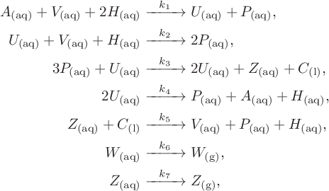 $$ \begin{align*} A_{(\mathrm{aq})}+V_{(\mathrm{aq})}+2H_{(\mathrm{aq})} &\xrightarrow{\;\;\;k_1\;\;\;}U_{(\mathrm{aq})}+P_{(\mathrm{aq})},\\ U_{(\mathrm{aq})}+V_{(\mathrm{aq})}+H_{(\mathrm{aq})}&\xrightarrow{\;\;\;k_2\;\;\;} 2P_{(\mathrm{aq})}, \\ 3P_{(\mathrm{aq})}+U_{(\mathrm{aq})}&\xrightarrow{\;\;\;k_3\;\;\;} 2U_{(\mathrm{aq})}+Z_{(\mathrm{aq})}+C_{(\mathrm{l})}, \\ 2U_{(\mathrm{aq})}&\xrightarrow{\;\;\;k_4\;\;\;} P_{(\mathrm{aq})}+A_{(\mathrm{aq})}+H_{(\mathrm{aq})}, \\ Z_{(\mathrm{aq})}+C_{(\mathrm{l})}&\xrightarrow{\;\;\;k_5\;\;\;} V_{(\mathrm{aq})}+P_{(\mathrm{aq})}+H_{(\mathrm{aq})},\\ W_{(\mathrm{aq})}&\xrightarrow{\;\;\;k_6\;\;\;} W_{(\mathrm{g})}, \\ Z_{(\mathrm{aq})}&\xrightarrow{\;\;\;k_7\;\;\;} Z_{(\mathrm{g})}, \end{align*} $$
where $k_1$
–
$k_1$
– $k_7$
denote various rate constants with values as prescribed in [Reference Dimsey, Forbes, Bassom and Quinn11], and the subscripts (l), (aq) and (g) indicate whether chemicals are in a liquid, aqueous or gaseous state as appropriate.
$k_7$
denote various rate constants with values as prescribed in [Reference Dimsey, Forbes, Bassom and Quinn11], and the subscripts (l), (aq) and (g) indicate whether chemicals are in a liquid, aqueous or gaseous state as appropriate.
It was demonstrated in [Reference Dimsey, Forbes, Bassom and Quinn11] that the key dynamics can be reduced to a set of four coupled equations for $U,V,W$
and Z. This was justified by appeal to the so-called pool approximation which was applied to the first four chemicals listed in Table 1. In essence, a pool approximation is appropriate when a chemical is present in sufficient quantity such that its concentration changes negligibly over the timescale of the reaction. Throughout the remainder of the paper we indicate when the pool approximation has been applied to a chemical species by designating its concentration as a parameter with the appropriate lower-case letter. Thus, for example, we shall apply the pool approximation to the concentration of water (variable C) and write its concentration as c.
$U,V,W$
and Z. This was justified by appeal to the so-called pool approximation which was applied to the first four chemicals listed in Table 1. In essence, a pool approximation is appropriate when a chemical is present in sufficient quantity such that its concentration changes negligibly over the timescale of the reaction. Throughout the remainder of the paper we indicate when the pool approximation has been applied to a chemical species by designating its concentration as a parameter with the appropriate lower-case letter. Thus, for example, we shall apply the pool approximation to the concentration of water (variable C) and write its concentration as c.
Some numerical simulations described in [Reference Dimsey, Forbes, Bassom and Quinn11] demonstrate how chemical oscillations can be set up which are reminiscent of those in the Bray–Liebhafsky model. Further analysis described in [Reference Dimsey, Forbes, Bassom and Quinn11] shows how the (already reduced) four-variable model can be simplified further to leave just a two-species system. This proved possible as the concentration of oxygen (W) within the four-variable system is independent of the values of the other three components and plays no active part in the fundamental dynamics. Moreover, the concentration of iodide (V) changes negligibly (compared to the other two variables on the relevant timescale) which allows a quasi-steady approximation to be implemented. This then leaves just a two-variable system given by
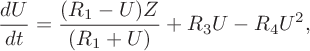 $$ \begin{align} \frac{dU}{dt} &= \frac{(R_1-U)Z}{(R_1+U)}+R_3U-R_4U^2, \end{align} $$
 $$ \begin{align} &\frac{dZ}{dt} = R_3U-(1+R_7) Z, \end{align} $$
for the concentrations of iodous acid (U) and iodine (Z). The evolution of these chemicals depends on the four dimensionless parameters $R_1$
,
$R_1$
, $R_3$
,
$R_3$
, $R_4$
and
$R_4$
and $R_7$
that are defined in Table 2. We note that the slightly peculiar numbering of these parameters is adopted since this preserves the notation used in [Reference Dimsey, Forbes, Bassom and Quinn11].
$R_7$
that are defined in Table 2. We note that the slightly peculiar numbering of these parameters is adopted since this preserves the notation used in [Reference Dimsey, Forbes, Bassom and Quinn11].
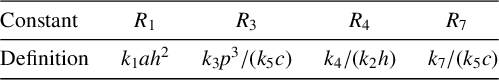
Table 2 Definitions of the dimensionless parameters within system (2.1). The values $a,c, h$
and p denote the (constant) pool concentrations of iodate, water, hydrogen ions and hypoiodous acid, respectively.
$a,c, h$
and p denote the (constant) pool concentrations of iodate, water, hydrogen ions and hypoiodous acid, respectively.
Within system (2.1) the time and concentrations have been rendered dimensionless based on $T_s = 1/(k_5c)$
and
$T_s = 1/(k_5c)$
and $M_s=1/(k_2h)$
, respectively; the reader is reminded that c and h denote the pool concentrations of water and hydrogen ions. This choice was made as it allowed other parameters to be set to unity in [Reference Dimsey, Forbes, Bassom and Quinn11]. It should be noted that throughout this paper
$M_s=1/(k_2h)$
, respectively; the reader is reminded that c and h denote the pool concentrations of water and hydrogen ions. This choice was made as it allowed other parameters to be set to unity in [Reference Dimsey, Forbes, Bassom and Quinn11]. It should be noted that throughout this paper $R_1$
and
$R_1$
and $R_4$
are held constant in all calculations with
$R_4$
are held constant in all calculations with $R_1 = 4.58\times 10^{-2}$
and
$R_1 = 4.58\times 10^{-2}$
and $R_4 = 1.68\times 10^{-3}$
. These values are based upon typical rate constants
$R_4 = 1.68\times 10^{-3}$
. These values are based upon typical rate constants $k_i$
derived from the literature [Reference De Kepper and Epstein10, Reference Lengyel, Li, Kustin and Epstein19, Reference Noyes and Furrow25] and initial conditions for our pool chemicals which were
$k_i$
derived from the literature [Reference De Kepper and Epstein10, Reference Lengyel, Li, Kustin and Epstein19, Reference Noyes and Furrow25] and initial conditions for our pool chemicals which were $a=0.02 \,M, c=55.5 \,M, h=0.04 \,M$
and
$a=0.02 \,M, c=55.5 \,M, h=0.04 \,M$
and $p=0.01\,M$
, where M is the concentration of each chemical in moles per litre. We were unable to find values for
$p=0.01\,M$
, where M is the concentration of each chemical in moles per litre. We were unable to find values for $k_3$
(due to being a “lumped” reaction step made of many elementary reactions) and
$k_3$
(due to being a “lumped” reaction step made of many elementary reactions) and $k_7$
. In consequence, we proceeded to adopt
$k_7$
. In consequence, we proceeded to adopt $R_3$
and
$R_3$
and $R_7$
as suitable bifurcation parameters as they proved the easiest to vary. Experimentally, these would be varied by changing the initial condition concentrations or varying the temperature, thus changing the rate constants.
$R_7$
as suitable bifurcation parameters as they proved the easiest to vary. Experimentally, these would be varied by changing the initial condition concentrations or varying the temperature, thus changing the rate constants.
Model (2.1) is a canonically simple autonomous system that can be analysed mathematically in the two-dimensional $(U,Z)$
phase plane. In [Reference Dimsey, Forbes, Bassom and Quinn11] we were able to identify regions in
$(U,Z)$
phase plane. In [Reference Dimsey, Forbes, Bassom and Quinn11] we were able to identify regions in $R_3$
–
$R_3$
– $R_7$
parameter space in which limit cycle behaviour is possible; physically this corresponds to the existence of sustained oscillations, which is qualitatively consistent with the experimental behaviour reported in [Reference Vukojević, Anić and Kolar-Anić31].
$R_7$
parameter space in which limit cycle behaviour is possible; physically this corresponds to the existence of sustained oscillations, which is qualitatively consistent with the experimental behaviour reported in [Reference Vukojević, Anić and Kolar-Anić31].
3 Formulation
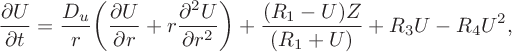
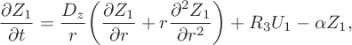
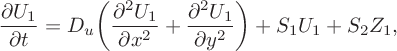
A key outcome of the study [Reference Dimsey, Forbes, Bassom and Quinn11] was the demonstration that the two-variable model given by system (2.1) is capable of generating temporal oscillations in the chemical system. Furthermore, these oscillations were shown to be consistent with those obtained from the full four-variable system of equations derived in [Reference Dimsey, Forbes, Bassom and Quinn11]. In order to introduce a spatial component we supplement the two-variable model with diffusion terms to give the system of partial differential equations (PDEs)
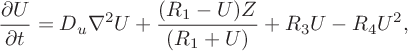 $$ \begin{align} \frac{\partial U}{\partial t} &= D _u\nabla^2 U+\frac{(R_1-U)Z}{(R_1+U)}+R_3U-R_4U^2, \end{align} $$
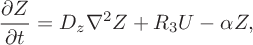 $$ \begin{align} &\frac{\partial Z}{\partial t} = D_z\nabla^2 Z+R_3U-\alpha Z, \end{align} $$
in which $D_u$
and
$D_u$
and $D_z$
are diffusion constants and
$D_z$
are diffusion constants and $\alpha \equiv 1+R_7$
.
$\alpha \equiv 1+R_7$
.
Throughout this paper, unless otherwise stated, we have chosen the dimensionless values $D_u=5\times 10^{-3}$
and
$D_u=5\times 10^{-3}$
and $D_z=10^{-2}$
for the diffusion constants. These values correspond to dimensional values of around
$D_z=10^{-2}$
for the diffusion constants. These values correspond to dimensional values of around $10^{-6}\,\mathrm {m}^2\mathrm {s}^{-1}$
. This choice was made for computational convenience despite the fact that the diffusion of iodide in water is accepted to lie in the range
$10^{-6}\,\mathrm {m}^2\mathrm {s}^{-1}$
. This choice was made for computational convenience despite the fact that the diffusion of iodide in water is accepted to lie in the range $O(10^{-9})\, \mathrm {m}^2\mathrm {s}^{-1}$
[Reference Cantrel, Chaouche and Chopin-Dumas7] at standard laboratory conditions (SLC) which correspond to a temperature of
$O(10^{-9})\, \mathrm {m}^2\mathrm {s}^{-1}$
[Reference Cantrel, Chaouche and Chopin-Dumas7] at standard laboratory conditions (SLC) which correspond to a temperature of $25^{\circ }$
C and a pressure of 1 atmosphere.
$25^{\circ }$
C and a pressure of 1 atmosphere.
We discuss the effect of reducing the diffusion coefficient towards more physical values later in the text. However, we suggest that this value may not be unduly unrealistic as it is very close to the kinematic viscosity coefficient of water at SLC which is reported to be $0.897\times 10^{-6}\,\mathrm {m}^2\mathrm {s}^{-1}$
[Reference Batchelor1]. In practice, we initiate our reaction by mixing a steady state with a solution of iodine. Consequently, it is not unreasonable to suppose that the early-time solutions are controlled by spreading via viscous processes. When we nondimensionalize using the chosen timescale and the lengthscale
$0.897\times 10^{-6}\,\mathrm {m}^2\mathrm {s}^{-1}$
[Reference Batchelor1]. In practice, we initiate our reaction by mixing a steady state with a solution of iodine. Consequently, it is not unreasonable to suppose that the early-time solutions are controlled by spreading via viscous processes. When we nondimensionalize using the chosen timescale and the lengthscale $L_s=5\times 10^{-2}\,\mathrm {m}$
, this gives our estimate for
$L_s=5\times 10^{-2}\,\mathrm {m}$
, this gives our estimate for $D_z$
. Therefore, while a more appropriate term for our diffusion coefficient might be a mixing coefficient (as it accounts for multiple spreading processes beyond pure molecular diffusion) we shall continue to refer to it as a diffusion coefficient throughout this work for consistency, since diffusion remains the dominant mechanism in the long term.
$D_z$
. Therefore, while a more appropriate term for our diffusion coefficient might be a mixing coefficient (as it accounts for multiple spreading processes beyond pure molecular diffusion) we shall continue to refer to it as a diffusion coefficient throughout this work for consistency, since diffusion remains the dominant mechanism in the long term.
Furthermore, we assume $D_u = 0.5D_z$
as it is widely accepted that Turing pattern formation requires that the diffusion coefficients are not equal (see Murray [Reference Murray23, Section 14.2]). Moreover, there does not appear to be any readily available published data relating to the size of the diffusion coefficient for iodous acid in water. Therefore, it seemed reasonable to assume
$D_u = 0.5D_z$
as it is widely accepted that Turing pattern formation requires that the diffusion coefficients are not equal (see Murray [Reference Murray23, Section 14.2]). Moreover, there does not appear to be any readily available published data relating to the size of the diffusion coefficient for iodous acid in water. Therefore, it seemed reasonable to assume $D_z>D_u$
; the motivation for this can be ascribed to the particular chemical properties of
$D_z>D_u$
; the motivation for this can be ascribed to the particular chemical properties of $\mathrm {I}_2$
molecules. These are small, have a linear geometry (as opposed to the bent shape of iodous acid which hinders diffusion) and do not undergo hydrogen bonding. As a result,
$\mathrm {I}_2$
molecules. These are small, have a linear geometry (as opposed to the bent shape of iodous acid which hinders diffusion) and do not undergo hydrogen bonding. As a result, $\mathrm {I}_2$
molecules should diffuse through solution at a faster rate than the bulkier
$\mathrm {I}_2$
molecules should diffuse through solution at a faster rate than the bulkier $\mathrm {H}\mathrm {I}\mathrm {O}_2$
ones. This becomes a significantly more difficult argument to make if we are truly considering kinematic viscosity as there does not appear to be any experimental data related to these measurements. However, the lack of experimental data for kinematic viscosity is not a significant issue in this context, as the process under consideration is not primarily governed by viscous effects.
$\mathrm {H}\mathrm {I}\mathrm {O}_2$
ones. This becomes a significantly more difficult argument to make if we are truly considering kinematic viscosity as there does not appear to be any experimental data related to these measurements. However, the lack of experimental data for kinematic viscosity is not a significant issue in this context, as the process under consideration is not primarily governed by viscous effects.
Typical practical equipment (such as beakers, Petri dishes and round-bottom flasks) is generally circular. It is therefore natural to write our problem in standard polar coordinates $(r,\theta )$
; we scale r by the radius of the container so its edge is at
$(r,\theta )$
; we scale r by the radius of the container so its edge is at $r=1$
. We note here that when this type of reaction is conducted in the laboratory with the aim of observing spatial patterns, a very thin film of solution (less than 1 cm thick) is normally used. This is done in order to avoid the effects of gas evolution and justifies the fact that we approximate our problem as two-dimensional. We begin with the simplest form of the problem in which we suppose the solution is radially symmetric so that
$r=1$
. We note here that when this type of reaction is conducted in the laboratory with the aim of observing spatial patterns, a very thin film of solution (less than 1 cm thick) is normally used. This is done in order to avoid the effects of gas evolution and justifies the fact that we approximate our problem as two-dimensional. We begin with the simplest form of the problem in which we suppose the solution is radially symmetric so that $U=U(r,t)$
and
$U=U(r,t)$
and $Z=Z(r,t)$
. Our system of nondimensionalized equations (3.1) then becomes
$Z=Z(r,t)$
. Our system of nondimensionalized equations (3.1) then becomes
 $$ \begin{align} \frac{\partial U}{\partial t} &= \frac{D_u}{r}\bigg(\frac{\partial U}{\partial r}+ r\frac{\partial ^2 U}{\partial r^2}\bigg) +\frac{(R_1-U)Z}{(R_1+U)}+R_3U-R_4U^2,\end{align} $$
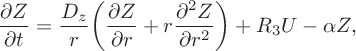 $$ \begin{align} &\frac{\partial Z}{\partial t} = \frac{D_z}{r} \bigg(\frac{\partial Z}{\partial r}+r\frac{\partial ^2 Z}{\partial r^2}\bigg) +R_3U-\alpha Z, \end{align} $$
which we shall refer to as the spatially extended model. We need to impose suitable conditions at $r=1$
, and these follow from the fact that there can be no chemical flux across the edge of the domain. Hence we claim that
$r=1$
, and these follow from the fact that there can be no chemical flux across the edge of the domain. Hence we claim that
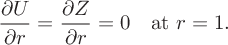 $$ \begin{align} \frac{\partial U}{\partial r}=\frac{\partial Z}{\partial r} =0\quad\mathrm{at}\ r=1. \end{align} $$
Finally, regularity conditions at the centre of coordinates imply that
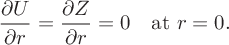 $$ \begin{align*} \frac{\partial U}{\partial r}= \frac{\partial Z}{\partial r}=0\quad\mathrm{at}\ r=0.\end{align*} $$
4 Linearized theory for circular patterns
We commence our analysis by finding the spatially homogeneous steady-state solutions of the system. It was shown in [Reference Dimsey, Forbes, Bassom and Quinn11] that the equilibrium solution to the corresponding ordinary differential equation system (2.1) is given by $U=U^*$
and
$U=U^*$
and $Z=Z^*$
, where
$Z=Z^*$
, where
 $$ \begin{align*}U^* = \frac{1}{2F}[-G+\sqrt{G^2+4FH}\,]\quad\mathrm{and}\quad Z^*= \frac{R_3U^*}{\alpha},\end{align*} $$
in which
 $$ \begin{align*} F\equiv R_4 \alpha ,\quad G\equiv R_1 R_4 \alpha -R_3R_7\quad\mathrm{and} \quad H\equiv R_1R_3(\alpha+1).\end{align*} $$
As this solution is spatially independent, it holds everywhere and is also a solution to the system of PDEs (3.2).
We develop a linearized approximation to the full system (3.2) by considering a small perturbation to the steady state of the form
 $$ \begin{align*}(U,Z)=(U^*,Z^*)+\delta( U_1(r,t), Z_1(r,t)) +\mathcal{O}(\delta^2),\quad |\delta|\ll 1.\end{align*} $$
Here, the small parameter $\delta $
gives a measure of the amplitude of the spatial patterns.
$\delta $
gives a measure of the amplitude of the spatial patterns.
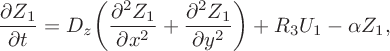
The spatially extended model (3.2) yields the approximate linearized system
 $$ \begin{align} \frac{\partial U_1}{\partial t} &= \frac{D_u}{r}\bigg(\frac{\partial U_1}{\partial r}+ r\frac{\partial ^2 U_1}{\partial r^2}\bigg)+S_1U_1 +S_2Z_1, \end{align} $$
 $$ \begin{align} \frac{\partial Z_1}{\partial t} = \frac{D_z}{r}& \bigg(\frac{\partial Z_1}{\partial r}+ r\frac{\partial ^2 Z_1}{\partial r^2}\bigg)+R_3U_1-\alpha Z_1, \end{align} $$
in which we have defined the constants
 $$ \begin{align} S_1 = -\frac{2R_1Z^*}{(R_1+U^*)^2}+R_3-2R_4U^*\quad\textrm{and} \quad S_2 = \bigg(\frac{R_1-U^*}{R_1+U^*}\bigg). \end{align} $$
The aim is to find the perturbation functions $U_1$
and
$U_1$
and $Z_1$
.
$Z_1$
.
We can solve system (4.1) using Laplace transforms with initial conditions $U_1(r,0)=0$
and
$U_1(r,0)=0$
and $Z_1(r,0)=F(r),$
where the function
$Z_1(r,0)=F(r),$
where the function $F(r)$
will be chosen conveniently in due course. Then with the definitions
$F(r)$
will be chosen conveniently in due course. Then with the definitions
 $$ \begin{align*}\widetilde{U}(r;s)=\int^\infty_0U_1(r,t)e^{-st}\,dt, \quad \widetilde{Z}(r;s)=\int^\infty_0Z_1(r,t)e^{-st}\,dt,\end{align*} $$
the Laplace transform of system (4.1) yields
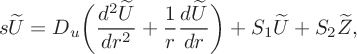 $$ \begin{align} &s\widetilde{U}=D _u\bigg(\frac{d^2\widetilde{U}}{dr^2}+ \frac{1}{r}\frac{d\widetilde{U}}{dr}\bigg)+S_1\widetilde{U}+S_2\widetilde{Z}, \end{align} $$
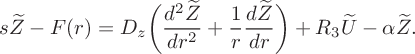 $$ \begin{align} &s\widetilde{Z}-F(r)= D _z\bigg(\frac{d^2\widetilde{Z}}{dr^2}+\frac{1}{r} \frac{d\widetilde{Z}}{dr}\bigg)+R_3\widetilde{U}-\alpha\widetilde{Z}. \end{align} $$
The structure of the differential operators in equations (4.3) suggests that we seek a solution
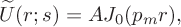 $$ \begin{align*} \widetilde{U}(r;s)=AJ_0(p_mr), \end{align*} $$
where $p_m$
is the mth zero of the Bessel function
$p_m$
is the mth zero of the Bessel function $J_1(z)=-J_0'(z)$
; this value is fixed by the requirement (3.3) that
$J_1(z)=-J_0'(z)$
; this value is fixed by the requirement (3.3) that $U_r=0$
at
$U_r=0$
at $r=1$
. With this, equation (4.3a) can be used to deduce that
$r=1$
. With this, equation (4.3a) can be used to deduce that
 $$ \begin{align*} \widetilde{Z}(r;s) = \frac{A}{S_2}(p_mD_u+s-S_1) J_0(p_m r) \end{align*} $$
with the constants $S_1$
and
$S_1$
and $S_2$
already given in (4.2). Then equation (4.3b) suggests that an appropriate, convenient form for the initial profile is
$S_2$
already given in (4.2). Then equation (4.3b) suggests that an appropriate, convenient form for the initial profile is $F(r)\equiv kJ_0(p_m r)$
where k is an arbitrary scaling constant. Assembling these results yields the solution
$F(r)\equiv kJ_0(p_m r)$
where k is an arbitrary scaling constant. Assembling these results yields the solution
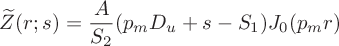
 $$ \begin{align*} &\widetilde{U}(r;s)=\frac{k S_2J_0(p_mr)}{s^2+s(\xi _1 +\xi _2) +(\xi_1\xi_2-S_2R_3)}, \\[10 pt] &\widetilde{Z}(r;s) = \frac{k(D _u p_m^2+s-S_1) J_0(p_mr)} {s^2+s(\xi_1+\xi_2)+(\xi_1\xi_2-S_2R_3)}, \end{align*} $$
in which $\xi _{1} \equiv p_m^2D_u -S_1$
and
$\xi _{1} \equiv p_m^2D_u -S_1$
and $ \xi _{2}\equiv p_m^2D_z+\alpha $
. If we denote the roots of the denominator of these expressions by
$ \xi _{2}\equiv p_m^2D_z+\alpha $
. If we denote the roots of the denominator of these expressions by $\mu _1$
and
$\mu _1$
and $\mu _2$
it follows that
$\mu _2$
it follows that
 $$ \begin{align} \mu_{1,2} = \tfrac{1}{2}\Big(-(\xi_1+\xi_2)\pm \sqrt{(\xi_1+\xi_2)^2-4(\xi_1\xi_2-S_2R_3)}\,\Big), \end{align} $$
and we can invert the Laplace transforms to deduce
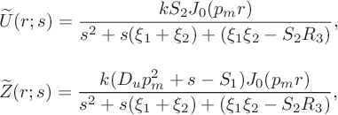
 $$ \begin{align} U_1(r,t) &= kS_2J_0(p_mr)\bigg[\frac{1}{\mu_1-\mu_2}\bigg] (e^{\mu_1t}-e^{\mu_2t}),\end{align} $$
 $$ \begin{align} &Z_1(r,t) = kJ_0(p_mr)\bigg[\bigg(\frac{\xi_1+\mu_1}{\mu_1-\mu_2}\bigg) e^{\mu_1t}-\bigg(\frac{\xi_1+\mu_2}{\mu_1-\mu_2}\bigg)e^{\mu_2t}\bigg]. \end{align} $$
An analysis of the linearized system (4.5) shows that the system is neutrally stable if both eigenvalues are purely imaginary: $\mathrm {Re}\{\mu _1\}=\mathrm {Re}\{\mu _2\}=0$
. From (4.4) this can be reduced to the relatively simple requirement that
$\mathrm {Re}\{\mu _1\}=\mathrm {Re}\{\mu _2\}=0$
. From (4.4) this can be reduced to the relatively simple requirement that
 $$ \begin{align} \xi_1+\xi_2\equiv p_m^2(D_u+D_z)+(\alpha-S_1)=0. \end{align} $$
If both the product $R_1R_4$
is small and also
$R_1R_4$
is small and also $R_3>1$
, then condition (4.6) guarantees that
$R_3>1$
, then condition (4.6) guarantees that $\mu _{1,2}$
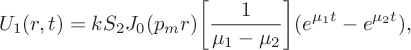
in (4.4) are purely imaginary, so that the solution (4.5) is neutrally stable. These results were also confirmed using numerical methods. The solution of (4.6) for various values of m is illustrated in Figure 1. Here, a two-parameter continuation of the Hopf bifurcation curves (where limit cycle oscillations are born in the nonlinear case; see [Reference Gray and Scott15]) has been performed in
$\mu _{1,2}$
in (4.4) are purely imaginary, so that the solution (4.5) is neutrally stable. These results were also confirmed using numerical methods. The solution of (4.6) for various values of m is illustrated in Figure 1. Here, a two-parameter continuation of the Hopf bifurcation curves (where limit cycle oscillations are born in the nonlinear case; see [Reference Gray and Scott15]) has been performed in $R_7$
–
$R_7$
– $R_3$
parameter space. Each line in this figure denotes where an individual mode undergoes a Hopf bifurcation and switches from being stable to unstable. They therefore mark the boundary between the stable and unstable regions in two-parameter space; below the
$R_3$
parameter space. Each line in this figure denotes where an individual mode undergoes a Hopf bifurcation and switches from being stable to unstable. They therefore mark the boundary between the stable and unstable regions in two-parameter space; below the $m=1$
line all modes of our series are stable. Therefore, in this region no mode will provide a growing contribution and any perturbation will be expected to return to the steady state. The unstable modes play a crucial role in enabling the pattern to emerge from the homogeneous steady state. In the linear case, these modes grow indefinitely, whereas in the nonlinear case, we expect that their growth will be constrained by nonlinear terms, thereby enabling a stable pattern to form.
$m=1$
line all modes of our series are stable. Therefore, in this region no mode will provide a growing contribution and any perturbation will be expected to return to the steady state. The unstable modes play a crucial role in enabling the pattern to emerge from the homogeneous steady state. In the linear case, these modes grow indefinitely, whereas in the nonlinear case, we expect that their growth will be constrained by nonlinear terms, thereby enabling a stable pattern to form.
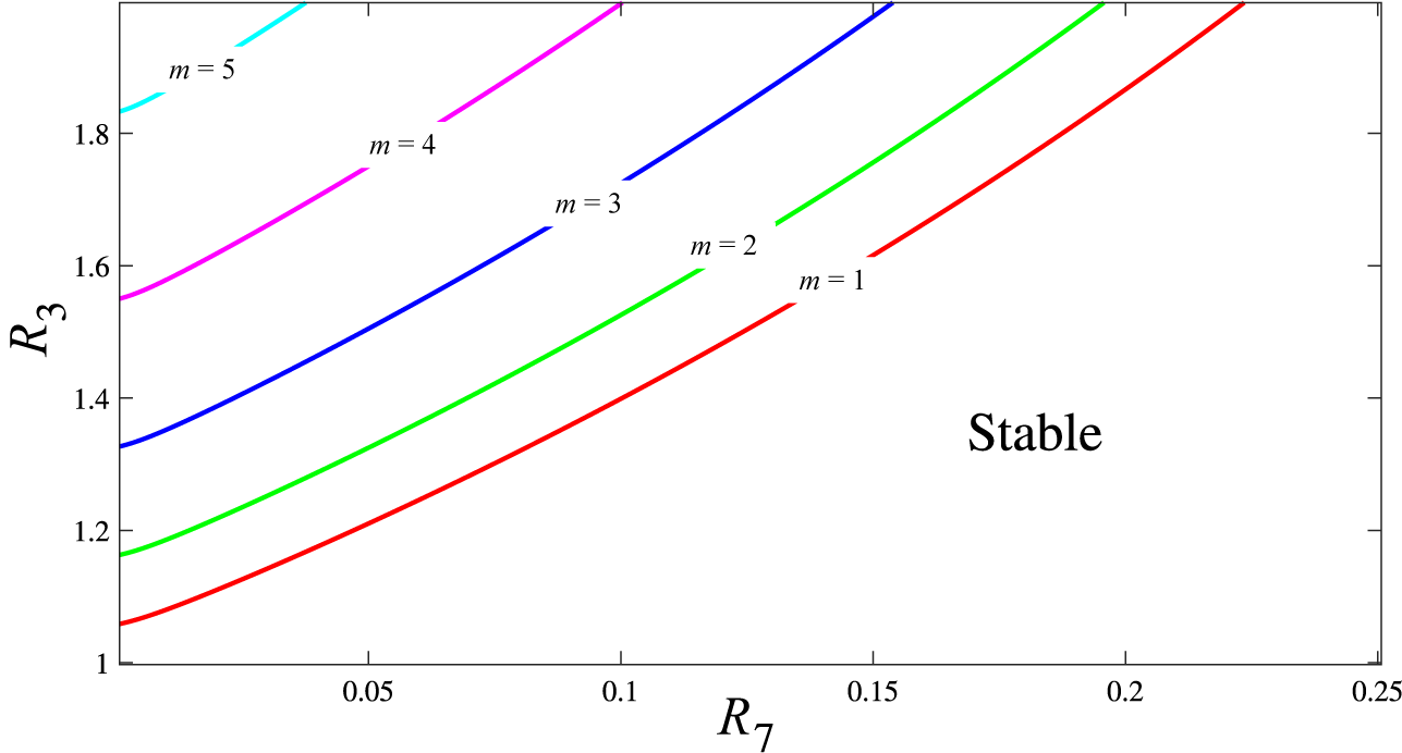
Figure 1 Bifurcation diagram in the $R_7$
–
$R_7$
– $R_3$
parameter space for the first five modes
$R_3$
parameter space for the first five modes $m=1, \ldots , 5$
. In the region between the lines
$m=1, \ldots , 5$
. In the region between the lines $m=j$
and
$m=j$
and $m=j+1$
the modes with
$m=j+1$
the modes with $m\leq j$
are linearly unstable and may be expected to exhibit nonlinear oscillatory behaviour. Here, we have
$m\leq j$
are linearly unstable and may be expected to exhibit nonlinear oscillatory behaviour. Here, we have $R_1 = 4.58\times 10^{-2}$
and
$R_1 = 4.58\times 10^{-2}$
and $R_4 = 1.68\times 10^{-3}$
.
$R_4 = 1.68\times 10^{-3}$
.
5 Nonlinear circular patterns
Given our exact linearized solution, we next proceed to consider solutions of the full nonlinear system (3.2). We begin by supposing that
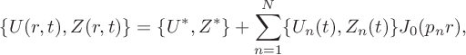 $$ \begin{align} \{U(r,t),Z(r,t) \}=\{U^*,Z^*\}+\sum_{n=1}^N\{U_n(t),Z_n(t) \}J_0(p_nr), \end{align} $$
which automatically satisfies the regularity conditions at the origin $r=0$
and the zero-flux condition (3.3) at the edge of the domain
$r=0$
and the zero-flux condition (3.3) at the edge of the domain $r=1$
. Expression (5.1) was substituted into the linear components of system (3.2), and then the standard Bessel orthogonality condition was applied to yield a set of differential equations for the Fourier coefficients. It follows that
$r=1$
. Expression (5.1) was substituted into the linear components of system (3.2), and then the standard Bessel orthogonality condition was applied to yield a set of differential equations for the Fourier coefficients. It follows that
 $$ \begin{align} \frac{dU_n(t)}{dt}=&-(D_u p_n^2-R_3)U_n(t) +\frac{2}{J_0^2(p_n)}\int_0^1 rJ_0(p_nr)\bigg[\bigg(\frac{R_1-U}{R_1+U}\bigg)Z -R_4U^2\bigg]\,dr,\end{align} $$
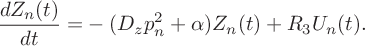 $$ \begin{align} \frac{dZ_n(t)}{dt} = &-(D_zp_n^2 +\alpha)Z_n(t)+R_3U_n(t). \end{align} $$
Clearly, this system requires numerical solution, and some suitable initial conditions need to be specified to enable this. We assume that $U(r,0)$
is the steady-state solution
$U(r,0)$
is the steady-state solution $U^*$
, while the component Z is perturbed so that
$U^*$
, while the component Z is perturbed so that $Z(r,0)=Z^*+h(r)$
. When these are substituted into expression (5.1), we deduce that
$Z(r,0)=Z^*+h(r)$
. When these are substituted into expression (5.1), we deduce that $U_n(0)=0$
and
$U_n(0)=0$
and
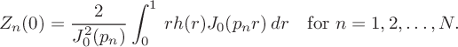 $$ \begin{align*} Z_n(0) = \frac{2}{J_0^2(p_n)}\int_0^1\,rh(r)J_0(p_nr)\,dr\quad\text{for } n=1,2,\ldots,N. \end{align*} $$
The next issue concerns the form of the initial function $h(r)$
. While there are several options available, we are motivated by thinking as to how the reaction might plausibly be initiated within a laboratory setting. We suppose that the steady state is perturbed by dropping some iodine to form a circle of finite radius (
$h(r)$
. While there are several options available, we are motivated by thinking as to how the reaction might plausibly be initiated within a laboratory setting. We suppose that the steady state is perturbed by dropping some iodine to form a circle of finite radius ( $r_c<1$
) near the centre of the container. This then suggests that a reasonable choice for the initial function
$r_c<1$
) near the centre of the container. This then suggests that a reasonable choice for the initial function $h(r)$
could be a simple unit step of the form
$h(r)$
could be a simple unit step of the form
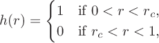 $$ \begin{align} h(r) = \begin{cases} 1 & \text{if } 0 < r < r_c, \\ 0 & \text{if } r_c < r < 1, \end{cases} \end{align} $$
where the value of $r_c$
is a measure of the size of the drop. While this profile can be explained from a practical viewpoint, it does present some computational issues associated with the discontinuity in
$r_c$
is a measure of the size of the drop. While this profile can be explained from a practical viewpoint, it does present some computational issues associated with the discontinuity in $h(r)$
. The implementation of a Fourier–Bessel series to represent this form of initial condition inevitably gives rise to the emergence of a Gibbs-type phenomenon (see [Reference Kreyszig, Kreyszig and Norminton17]), leading to spurious oscillations in the reconstructed concentration profiles, associated with the discontinuity in (5.3) at
$h(r)$
. The implementation of a Fourier–Bessel series to represent this form of initial condition inevitably gives rise to the emergence of a Gibbs-type phenomenon (see [Reference Kreyszig, Kreyszig and Norminton17]), leading to spurious oscillations in the reconstructed concentration profiles, associated with the discontinuity in (5.3) at $r=r_c$
. In order to mitigate this effect it proved useful to conduct our calculations in combination with a suitable smoothing technique. We chose to apply Lanczos smoothing (filtering) to the initial condition in which each coefficient within the Fourier series is multiplied by a suitable smoothing constant as described in [Reference Duchon12]. In particular, the nth Fourier coefficient was multiplied by the sinc function defined by
$r=r_c$
. In order to mitigate this effect it proved useful to conduct our calculations in combination with a suitable smoothing technique. We chose to apply Lanczos smoothing (filtering) to the initial condition in which each coefficient within the Fourier series is multiplied by a suitable smoothing constant as described in [Reference Duchon12]. In particular, the nth Fourier coefficient was multiplied by the sinc function defined by
 $$ \begin{align*}\textrm{sinc}(n\sigma) = \frac{\sin(n\sigma)}{n\sigma},\quad n = 1,2,\ldots,N,\end{align*} $$
where $\sigma $
is a prescribed smoothing constant, referred to as the Lanczos parameter. In general, larger values of
$\sigma $
is a prescribed smoothing constant, referred to as the Lanczos parameter. In general, larger values of $\sigma $
tend to give smoother functions, with the trade-off that as
$\sigma $
tend to give smoother functions, with the trade-off that as $\sigma $
grows so the smoothed function increasingly deviates from the original. With some trial and error we found that modifying the initial condition with
$\sigma $
grows so the smoothed function increasingly deviates from the original. With some trial and error we found that modifying the initial condition with $\sigma $
somewhere in the interval
$\sigma $
somewhere in the interval $(0.06, 0.15)$
appeared to give the best compromise between smoothness and trueness to the original function. Ultimately, the value of
$(0.06, 0.15)$
appeared to give the best compromise between smoothness and trueness to the original function. Ultimately, the value of $\sigma $
did not change the final state reached.
$\sigma $
did not change the final state reached.
The evolution equations (5.2) were numerically integrated forward in time using the standard ode45 package within the MATLAB suite of routines, which is an adaptive timestep Runge–Kutta method that uses fourth- and fifth-order accurate solutions to control the error by varying each timestep. Other integrators specifically designed for integrating stiff functions were also trialled but these did not perform discernibly any better. We divided the entire integration run into a number of sub-intervals (typically each of duration $1$
–
$1$
– $100$
dimensionless time units) as this allowed us to monitor the evolution of the pattern.
$100$
dimensionless time units) as this allowed us to monitor the evolution of the pattern.
With the smoothed shape function (5.3) used as the initial condition, we were able to compute some basic spatial patterns. Various tests were conducted, including using a selection of initial conditions, choosing different durations for the time sub-intervals (which modified the computational time used to reach a solution) and the number of terms N retained in the Fourier expansion (5.1). It was notable that (for a prescribed set of parameter values) the precise choice of initial profiles for U and Z seemed to have minimal effect on the final profile or the rate at which these structures were attained. Some sample results are illustrated in Figure 2, for the nonlinear solution (5.1) using $N=51$
Fourier coefficients and the parameters
$N=51$
Fourier coefficients and the parameters $\sigma =0.11$
,
$\sigma =0.11$
, $R_7=0.015$
,
$R_7=0.015$
, $R_3=1.0920$
,
$R_3=1.0920$
, $r_c=0.1$
,
$r_c=0.1$
, $D_u=5\times 10^{-3}$
and
$D_u=5\times 10^{-3}$
and $D_z=1\times 10^{-2}$
. These solutions show the emergence of a steady pattern at relatively early times; we see that the final shape of the iodine concentration (Z) appears as early as about
$D_z=1\times 10^{-2}$
. These solutions show the emergence of a steady pattern at relatively early times; we see that the final shape of the iodine concentration (Z) appears as early as about $t=60$
and attains its long-term value by
$t=60$
and attains its long-term value by $t=100$
.
$t=100$
.
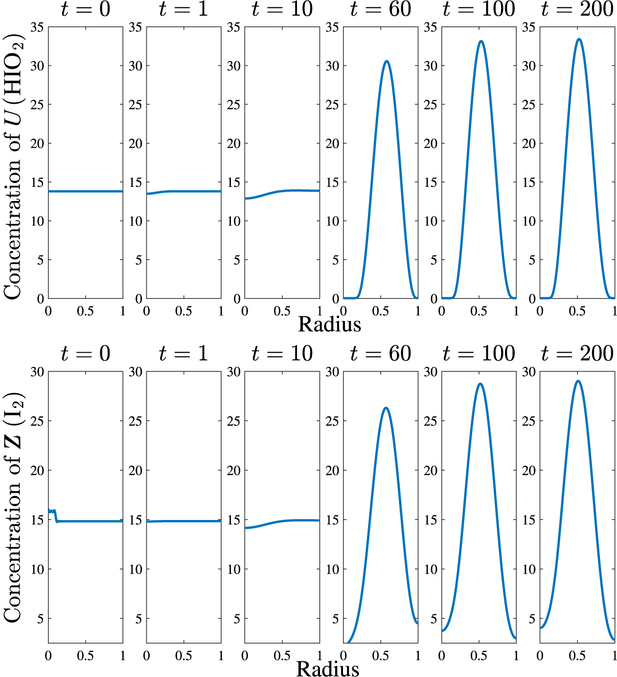
Figure 2 The evolution of the U-concentration (top) and Z-concentration (bottom) in a one-dimensional radially symmetric model using $N=51$
coefficients in the linearized equation (5.1). The parameter values were chosen to be
$N=51$
coefficients in the linearized equation (5.1). The parameter values were chosen to be $R_7=0.015$
,
$R_7=0.015$
, $R_3=1.0920$
, smoothing parameter
$R_3=1.0920$
, smoothing parameter $\sigma =0.11$
with an initial shape function of magnitude
$\sigma =0.11$
with an initial shape function of magnitude $1$
with
$1$
with $r_c=0.1$
. The diffusion coefficients used are
$r_c=0.1$
. The diffusion coefficients used are $D_u=5\times 10^{-3}$
and
$D_u=5\times 10^{-3}$
and $D_z=1\times 10^{-2}$
.
$D_z=1\times 10^{-2}$
.
We can take the final solutions from Figure 2 and then calculate the concentration of iodide (V) using the quasi-steady approximation
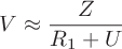 $$ \begin{align*}V\approx \frac{Z}{R_1+U}\end{align*} $$
noted in [Reference Dimsey, Forbes, Bassom and Quinn11]. Following this, a comparison of the magnitudes of the concentrations of iodine and iodide enables us to infer some properties of the respective spatial patterns. We depict this in Figure 3(a) where we have shown those regions, where the concentration of iodide is greater than iodine ( $V>Z$
) in blue and the alternative case (
$V>Z$
) in blue and the alternative case ( $V<Z$
) in red.
$V<Z$
) in red.
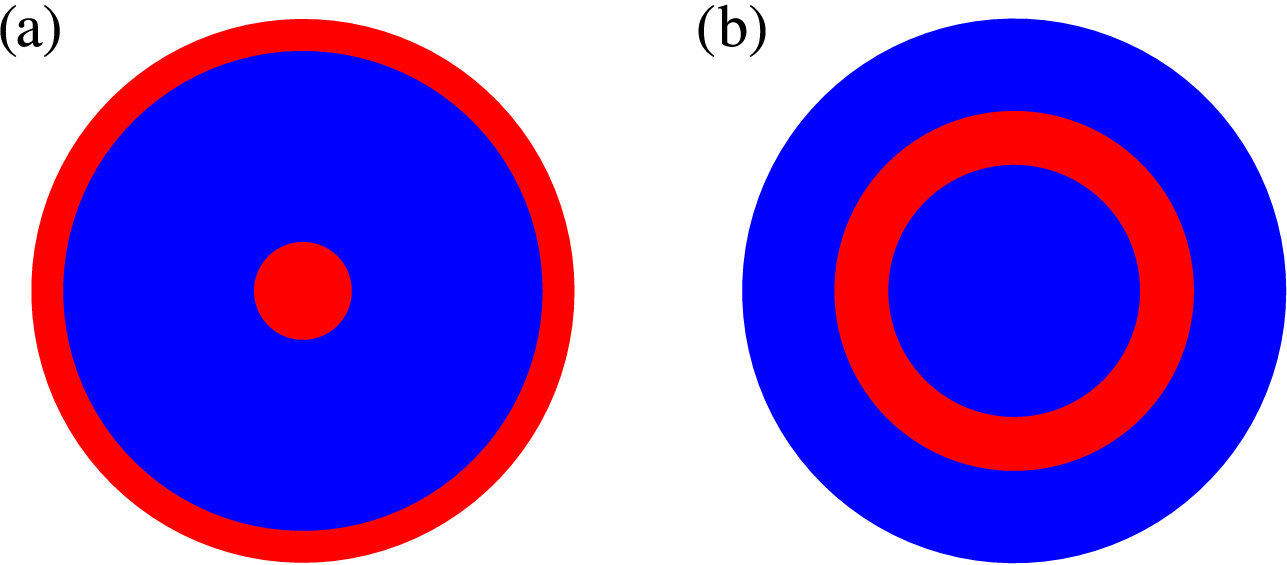
Figure 3 The patterns formed after long times for a range of radially symmetric initial conditions. Areas shaded red indicate where the concentration of Z exceeds that of V; where the reverse applies the area is blue. The pattern formed with the initial conditions of either (5.3), (5.4) with $m=1$
or (5.5) with either
$m=1$
or (5.5) with either $m=1$
or
$m=1$
or $m=2$
is shown in (a) and the initial condition (5.4) with
$m=2$
is shown in (a) and the initial condition (5.4) with $m=2$
is shown in (b). Numerical scheme used
$m=2$
is shown in (b). Numerical scheme used $N=51$
coefficients with parameter values
$N=51$
coefficients with parameter values $R_7=0.015$
,
$R_7=0.015$
, $R_3=1.0920$
, smoothing parameter
$R_3=1.0920$
, smoothing parameter $\sigma =0.11$
and diffusion coefficients
$\sigma =0.11$
and diffusion coefficients $D_u=5\times 10^{-3}$
and
$D_u=5\times 10^{-3}$
and $D_z=1\times 10^{-2}$
.
$D_z=1\times 10^{-2}$
.
Next, we took the initial condition $h(r)$
to be a simple cosine function of the form
$h(r)$
to be a simple cosine function of the form
 $$ \begin{align} h(r) = \cos (2m\pi r)\quad \text{where}\ m=1,2,\ldots. \end{align} $$
With $m=1$
the final pattern was precisely the same as that formed when the step-function initial condition (5.3) was used (see Figure 3(a)). It was noted that for any initial condition of this form with
$m=1$
the final pattern was precisely the same as that formed when the step-function initial condition (5.3) was used (see Figure 3(a)). It was noted that for any initial condition of this form with $m>1$
a different pattern emerged, leading us to believe that there are two possible steady patterns for this parameter combination. These steady patterns are illustrated in Figure 3 where we have shown the two patterns that arise. We tested a range of other parameter values within the unstable region of the parameter space and found exactly the same patterns regardless of the value of
$m>1$
a different pattern emerged, leading us to believe that there are two possible steady patterns for this parameter combination. These steady patterns are illustrated in Figure 3 where we have shown the two patterns that arise. We tested a range of other parameter values within the unstable region of the parameter space and found exactly the same patterns regardless of the value of $R_7$
.
$R_7$
.
Following on, we next tried adjusting the initial conditions to explore whether this extended the range of final configurations. Consequently, we perturbed the initial condition so that it took the general form
 $$ \begin{align} h(r)=\cos (2m\pi r)+0.1[\cos(2\pi r)+\cos(4 \pi r)] \quad \text{where } m=1,2,\ldots. \end{align} $$
We found that when $m=1$
in expression (5.5) nothing changed from the situation in which the perturbation is absent. By way of contrast, when
$m=1$
in expression (5.5) nothing changed from the situation in which the perturbation is absent. By way of contrast, when $m=2$
in (5.5) the final pattern is identical to that which arises when
$m=2$
in (5.5) the final pattern is identical to that which arises when $m=1$
in (5.4); this is shown in Figure 3(a). We comment that our experiments with various initial profiles seem to suggest that the pattern associated with the simple form (5.4) when
$m=1$
in (5.4); this is shown in Figure 3(a). We comment that our experiments with various initial profiles seem to suggest that the pattern associated with the simple form (5.4) when $m=1$
occurs most frequently. We can tentatively suggest that this
$m=1$
occurs most frequently. We can tentatively suggest that this $m=1$
steady pattern possesses a significantly larger basin of attraction. The upshot is that if we evolve a radially symmetric initial profile it is most likely that a pattern akin to that in Figure 3(a) appears.
$m=1$
steady pattern possesses a significantly larger basin of attraction. The upshot is that if we evolve a radially symmetric initial profile it is most likely that a pattern akin to that in Figure 3(a) appears.
It is worth mentioning that the fact that the pattern formed from the step function tends directly to the same steady pattern as is associated with the mode $1$
initial condition is no coincidence. This should be expected as the Fourier representation of the step function will have some contribution from the first mode. Therefore, it should tend directly to the
$1$
initial condition is no coincidence. This should be expected as the Fourier representation of the step function will have some contribution from the first mode. Therefore, it should tend directly to the $m=1$
steady pattern.
$m=1$
steady pattern.
It should be noted that all calculations discussed in this section lie within the parameter region in which only the first mode is unstable as shown in Figure 1. This helps explain why the observed patterns seem to have a dominant mode $1$
component. However, for other parameter selections, in particular ones for which the second and third modes are also linearly unstable, we found that the mode
$1$
component. However, for other parameter selections, in particular ones for which the second and third modes are also linearly unstable, we found that the mode $1$
component continued to be the most prominent. This leads us to speculate that the first mode may be the most unstable for this parameter combination. We observe that the nonlinearity of the governing PDE system means that even though the first mode might be linearly unstable, the nonlinear patterns will nevertheless not grow without bound. In this way, large-amplitude stable spatial patterns can form for parameter values at which small-amplitude patterns are unstable.
$1$
component continued to be the most prominent. This leads us to speculate that the first mode may be the most unstable for this parameter combination. We observe that the nonlinearity of the governing PDE system means that even though the first mode might be linearly unstable, the nonlinear patterns will nevertheless not grow without bound. In this way, large-amplitude stable spatial patterns can form for parameter values at which small-amplitude patterns are unstable.
6 Two-dimensional patterns
Having gained some understanding as to the possibilities for radially symmetric distributions, we now generalize our considerations to allow for some genuinely two-dimensional patterns that may emerge from our model. We remark that here we switch to a rectangular domain. This was done because our calculations of radially symmetric solutions in a circular domain began to run into computational problems, a phenomenon that could be ascribed to the increasing stiffness of the problem. Using Cartesian coordinates is particularly helpful in this regard as the adoption of this geometry enables straightforward vectorization, in our numerical evaluation of Fourier series and quadrature techniques, which markedly improves the overall efficiency of the code. Our equations were integrated over the domain $|x|\leq L$
,
$|x|\leq L$
, $|y|\leq B$
which defines a rectangular region of length
$|y|\leq B$
which defines a rectangular region of length $2L$
and width
$2L$
and width $2B$
. While rectangles are not particularly common shapes for glassware, they are occasionally used in both chemistry and biology experiments [Reference Yazdanbakhsh and Fisahn33]. The relevant Neumann boundary conditions can be written as
$2B$
. While rectangles are not particularly common shapes for glassware, they are occasionally used in both chemistry and biology experiments [Reference Yazdanbakhsh and Fisahn33]. The relevant Neumann boundary conditions can be written as
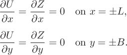 $$ \begin{align} \frac{\partial U}{\partial x} &= \frac{\partial Z}{\partial x}=0\quad \text{on}\ x=\pm L,\\[5pt]\frac{\partial U}{\partial y}&=\frac{\partial Z}{\partial y} =0 \quad \text{on}\ y=\pm B. \end{align} $$
Written in terms of Cartesian coordinates, the governing equations (3.1) can be cast as
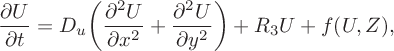 $$ \begin{align} \frac{\partial U}{\partial t} &= D_u\bigg(\frac{\partial ^2 U} {\partial x^2}+\frac{\partial^2 U}{\partial y^2}\bigg) +R_3U + f(U,Z), \end{align} $$
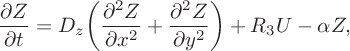 $$ \begin{align} &\frac{\partial Z}{\partial t} = D_z\bigg(\frac{\partial^2 Z} {\partial x^2}+\frac{\partial^2Z}{\partial y^2}\bigg)+R_3U-\alpha Z, \end{align} $$
in which all the nonlinear components are subsumed in the term
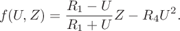 $$ \begin{align*}f(U,Z) = \frac{R_1-U}{R_1+U}Z-R_4U^2.\end{align*} $$
6.1 The linear model
We begin with the linearized problem defined by
 $$ \begin{align} \frac{\partial U_1}{\partial t} &= D _u\bigg(\frac{\partial ^2 U_1} {\partial x^2}+\frac{\partial ^2 U_1}{\partial y^2}\bigg)+S_1U_1 +S_2Z_1, \end{align} $$
 $$ \begin{align}\frac{\partial Z_1}{\partial t} &= D _z\bigg(\frac{\partial ^2 Z_1} {\partial x^2}+\frac{\partial ^2 Z_1}{\partial y^2}\bigg)+R_3U_1- \alpha Z_1, \end{align} $$
where the constants $S_1$
and
$S_1$
and $S_2$
are precisely as defined in (4.2). Guided by the boundary conditions (6.1) on
$S_2$
are precisely as defined in (4.2). Guided by the boundary conditions (6.1) on $x=\pm L$
,
$x=\pm L$
, $y=\pm B$
, we seek a linearized solution of the form
$y=\pm B$
, we seek a linearized solution of the form
 $$ \begin{align} &U_1(x,y,t) = \sum^\infty_{m=0}\sum^\infty_{n=0}A_{m,n}^L(t)\cos\bigg(\frac{m\pi(x+L)} {2L}\bigg)\cos\bigg(\frac{n\pi(y+B)}{2B}\bigg), \end{align} $$
 $$ \begin{align} &Z_1(x,y,t) = \sum^\infty_{m=0}\sum^\infty_{n=0}B_{m,n}^L(t)\cos\bigg(\frac{m\pi(x+L)} {2L}\bigg)\cos\bigg(\frac{n\pi(y+B)}{2B}\bigg). \end{align} $$
If we substitute the ansatz (6.4) into (6.3), and appeal to the orthogonality of cosines, we derive a system of differential equations for the coefficients given by
 $$ \begin{align} &\frac{d}{dt}A_{m,n}^L(t)=\bigg(-\frac14 D_u\pi^2\Gamma^2_{m,n}+S_1\bigg)\,A_{m,n}^L(t)+S_2B_{m,n}^L(t), \end{align} $$
 $$ \begin{align} &\!\kern-1pt \frac{d}{dt}B_{m,n}^L(t)= \bigg(-\frac14D_z\pi^2\Gamma^2_{m,n}- \alpha\bigg)\,B_{m,n}^L(t)+R_3A_{m,n}^L(t), \end{align} $$
in which we have defined
 $$ \begin{align*}\Gamma^2_{m,n} \equiv \bigg(\frac{m^2}{L^2}+\frac{n^2}{B^2}\bigg). \end{align*} $$
It is then a routine exercise to conclude that
 $$ \begin{align*} B_{m,n}^L(t)=B_1\exp(\lambda^+_{m,n}t)+B_2\exp(\lambda^-_{m,n}t), \quad B_1,B_2\in\mathcal{R}, \end{align*} $$
where the eigenvalues $\lambda _{m,n}^{\pm }$
are the solutions of the quadratic
$\lambda _{m,n}^{\pm }$
are the solutions of the quadratic
 $$ \begin{align*} \lambda^2+(\zeta_{m,n}+R_3\eta_{m,n})\lambda+R_3(\eta_{m,n}\zeta_{m,n}-S_2)=0 \end{align*} $$
with
 $$ \begin{align*}\eta_{m,n} \equiv \frac{D _u\pi^2}{4}\Gamma^2_{m,n}- S_1\quad\textrm{and}\quad\zeta_{m,n} \equiv \frac{D _z\pi^2} {4}\Gamma^2_{m,n}+\alpha.\end{align*} $$
Upon determining the solution coefficients $B_{m,n}^L$
, we can immediately deduce the form of
$B_{m,n}^L$
, we can immediately deduce the form of $A_{m,n}^L$
from equation (6.5b).
$A_{m,n}^L$
from equation (6.5b).
We have now derived the modal solution of the linearized problem. For general initial conditions $U(x,y,0) = F(x,y)$
and
$U(x,y,0) = F(x,y)$
and $Z(x,y,0) = G(x,y)$
, we can express the solutions as linear combinations of the modes, and determine the various coefficients by Fourier analysis in the usual way. In the interest of brevity, we do not write out all the details here.
$Z(x,y,0) = G(x,y)$
, we can express the solutions as linear combinations of the modes, and determine the various coefficients by Fourier analysis in the usual way. In the interest of brevity, we do not write out all the details here.
6.2 The nonlinear model
To develop the nonlinear solution we again begin with a series solution in which
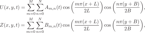 $$ \begin{align*} &U(x,y,t) = \sum^M_{m=0}\sum^N_{n=0}A_{m,n}(t)\cos\bigg(\frac{m\pi(x+L)} {2L}\bigg)\cos\bigg(\frac{n\pi(y+B)}{2B}\bigg), \\ &Z(x,y,t) = \sum^M_{m=0}\sum^N_{n=0}B_{m,n}(t)\cos\bigg(\frac{m\pi(x+L)} {2L}\bigg)\cos\bigg(\frac{n\pi(y+B)}{2B}\bigg), \end{align*} $$
for some coefficients $A_{m,n}(t)$
and
$A_{m,n}(t)$
and $B_{m,n}(t)$
. These series become more accurate as the numbers M and N of Fourier modes are increased. If we substitute these expressions into the linear components of system (6.2) and apply the cosine orthogonality conditions we deduce that
$B_{m,n}(t)$
. These series become more accurate as the numbers M and N of Fourier modes are increased. If we substitute these expressions into the linear components of system (6.2) and apply the cosine orthogonality conditions we deduce that
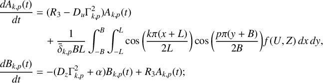 $$ \begin{align*} \frac{dA_{k,p}(t)}{dt} &= (R_3-D_u\Gamma^2_{k,p})A_{k,p}(t) \\&\quad +\frac{1}{\bar{\delta}_{k,p}BL}\int_{-B}^B\int_{-L}^L \cos\bigg(\frac{k\pi(x+L)}{2L}\bigg) \cos\bigg(\frac{p\pi(y+B)}{2B}\bigg)\,f(U,Z)\,dx\,dy, \\\frac{dB_{k,p}(t)}{dt} &= -(D_z\Gamma^2_{k,p}+\alpha)B_{k,p}(t) + R_3A_{k,p}(t); \end{align*} $$
here $\bar {\delta }_{0,0}=4$
,
$\bar {\delta }_{0,0}=4$
, $\bar {\delta }_{k,p}=2$
if either
$\bar {\delta }_{k,p}=2$
if either $k=0$
or
$k=0$
or $p=0$
and
$p=0$
and $\bar {\delta }_{k,p}=1$
otherwise.
$\bar {\delta }_{k,p}=1$
otherwise.
Once again, we need to specify initial values $A_{m,n}(0)$
and
$A_{m,n}(0)$
and $B_{m,n}(0)$
in order to evolve the equations in time. Fortunately, this choice does not critically affect the ultimate state of the system and, for simplicity, we supposed that
$B_{m,n}(0)$
in order to evolve the equations in time. Fortunately, this choice does not critically affect the ultimate state of the system and, for simplicity, we supposed that $U(x,y,0) = U^*$
and
$U(x,y,0) = U^*$
and $Z(x,y,0)=Z^*+G(x,y)$
. This corresponds to U and Z being at their equilibrium values before adding some excess iodine (Z). There are few constraints on
$Z(x,y,0)=Z^*+G(x,y)$
. This corresponds to U and Z being at their equilibrium values before adding some excess iodine (Z). There are few constraints on $G(x,y)$
except that it should satisfy (or nearly satisfy) the prescribed Neumann boundary conditions (6.1). Throughout our analysis we have worked with a range of initial conditions, including choosing
$G(x,y)$
except that it should satisfy (or nearly satisfy) the prescribed Neumann boundary conditions (6.1). Throughout our analysis we have worked with a range of initial conditions, including choosing $G(x,y)$
to be a quartic function, Bessel function, Gaussian, a product of cosines and a step function among others.
$G(x,y)$
to be a quartic function, Bessel function, Gaussian, a product of cosines and a step function among others.
These initial conditions imply that the only nonzero $A_{m,n}(0)$
is
$A_{m,n}(0)$
is $A_{0,0}(0) = U^*$
, while the
$A_{0,0}(0) = U^*$
, while the $B_{m,n}(0)$
are given by
$B_{m,n}(0)$
are given by
 $$ \begin{align*} B_{m,n}(0) = \frac{1}{\bar{\delta}_{m,n}BL}\int_{-B}^B\int_{-L}^LG(x,y)&\cos\bigg(\frac{m\pi(x+L)}{2L}\bigg)\times \cos\bigg(\frac{n\pi(y+B)}{2B}\bigg)\,dx\,dy. \end{align*} $$
Using a similar process to that outlined in Section 5 we are then able to integrate the system forward in time given a particular initial condition.
Most of the results we describe below were obtained using spectral methods. However, we also benchmarked our work by conducting a number of the calculations using techniques based on the method of lines. This is a finite-difference method which is commonly applied to integrate reaction–diffusion systems. Further details of our precise implementation of the method of lines have been relegated to Appendix A.
7 Results
A first step in our analysis of the two-dimensional system necessitates that we locate those parts of parameter space where interesting spatial patterning might arise. To enable this we created a bifurcation diagram based upon the Fourier transform of the system. In our previous results described in Section 5 we used $R_7$
and
$R_7$
and $R_3$
as our bifurcation parameters. Here we take an alternative view; we fix
$R_3$
as our bifurcation parameters. Here we take an alternative view; we fix $R_3=1.0920$
and adopt
$R_3=1.0920$
and adopt $R_7$
and the ratio of the diffusion constants as the bifurcation quantities. To this end we define the diffusion ratio
$R_7$
and the ratio of the diffusion constants as the bifurcation quantities. To this end we define the diffusion ratio $d \equiv D_u/D_z$
which can vary between
$d \equiv D_u/D_z$
which can vary between $0$
and
$0$
and $1$
. We then constructed the requisite bifurcation diagram using a somewhat inelegant “brute force” approach that is based on the eigenvalues of the linearized system in Section 6.1. This required us to calculate the eigenvalues, the fastest-growing mode and the associated behaviour for each parameter combination within our region of interest and then classify the nature of each eigenvalue combination in a similar manner to that outlined in [Reference Bois4]. If all modes had a negative real eigenvalue the system was designated stable as any perturbation would decay to the homogeneous equilibrium over time. On the other hand, if the eigenvalue of the zeroth mode is positive (and with a nonzero imaginary part) while all other modes have negative real parts, the solution sits in what we refer to as the homogeneous oscillatory region, where the concentration becomes spatially homogeneous but oscillates in magnitude over time. Finally, if the fastest-growing mode and the eigenvalues were both greater than zero then a spatial structure would be expected to form. The outcome of this is summarized in Figure 4. Three distinct regions appear in the d–
$1$
. We then constructed the requisite bifurcation diagram using a somewhat inelegant “brute force” approach that is based on the eigenvalues of the linearized system in Section 6.1. This required us to calculate the eigenvalues, the fastest-growing mode and the associated behaviour for each parameter combination within our region of interest and then classify the nature of each eigenvalue combination in a similar manner to that outlined in [Reference Bois4]. If all modes had a negative real eigenvalue the system was designated stable as any perturbation would decay to the homogeneous equilibrium over time. On the other hand, if the eigenvalue of the zeroth mode is positive (and with a nonzero imaginary part) while all other modes have negative real parts, the solution sits in what we refer to as the homogeneous oscillatory region, where the concentration becomes spatially homogeneous but oscillates in magnitude over time. Finally, if the fastest-growing mode and the eigenvalues were both greater than zero then a spatial structure would be expected to form. The outcome of this is summarized in Figure 4. Three distinct regions appear in the d– $R_7$
parameter space; it is the green shaded part of Figure 4 that is of most interest since this is where we predict the formation of spatial patterning.
$R_7$
parameter space; it is the green shaded part of Figure 4 that is of most interest since this is where we predict the formation of spatial patterning.
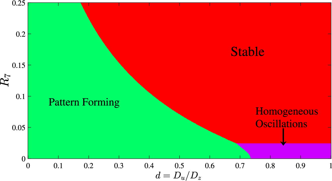
Figure 4 Spatial pattern bifurcation diagram in d– $R_7$
parameter space based on linearized analysis. Three distinct areas arise. For parameter choices in the red region the pattern returns to the homogeneous steady state; the green region indicates values at which Turing patterns form. Finally, when in the purple region the pattern settles to a spatially homogeneous value which oscillates in magnitude over time.
$R_7$
parameter space based on linearized analysis. Three distinct areas arise. For parameter choices in the red region the pattern returns to the homogeneous steady state; the green region indicates values at which Turing patterns form. Finally, when in the purple region the pattern settles to a spatially homogeneous value which oscillates in magnitude over time.
Given this preliminary linear stability analysis of the system, we next investigate the extension to nonlinear cases. We would expect to see close agreement between the linear and nonlinear simulations, at least for relatively small amplitude perturbations from the steady state and for early times. In all our comparisons we prescribe initial conditions defined by $U(x,y,0)=U_{ss}$
and
$U(x,y,0)=U_{ss}$
and
 $$ \begin{align} Z(x,y,0) = Z_{ss}+M\cos\bigg(\frac{2\pi (x+L)} {2L}\bigg)\cos\bigg(\frac{4\pi (y+B)}{2B}\bigg), \end{align} $$
where M is the magnitude of the perturbation function. In order to measure the difference in the linear and nonlinear results, we choose to look at the concentration profile of Z along the centre line $y=0$
of the dish. This type of initial condition, while not necessarily wholly physically realizable, was chosen as it closely resembles the assumed Fourier series solution in the spectral method.
$y=0$
of the dish. This type of initial condition, while not necessarily wholly physically realizable, was chosen as it closely resembles the assumed Fourier series solution in the spectral method.
Our first results are shown in Figure 5. Here we have $M=0.1$
and the pair of parameters
$M=0.1$
and the pair of parameters $d=0.5$
,
$d=0.5$
, $R_7=0.18$
which lies within the stable portion of parameter space in Figure 4. (In all comparisons the nonlinear equations were solved both spectrally and with the method of lines and the outcomes are identical at all times shown.) As would be expected the initial perturbation evolves nonlinearly over small times before decaying away to leave just the uniform steady state.
$R_7=0.18$
which lies within the stable portion of parameter space in Figure 4. (In all comparisons the nonlinear equations were solved both spectrally and with the method of lines and the outcomes are identical at all times shown.) As would be expected the initial perturbation evolves nonlinearly over small times before decaying away to leave just the uniform steady state.
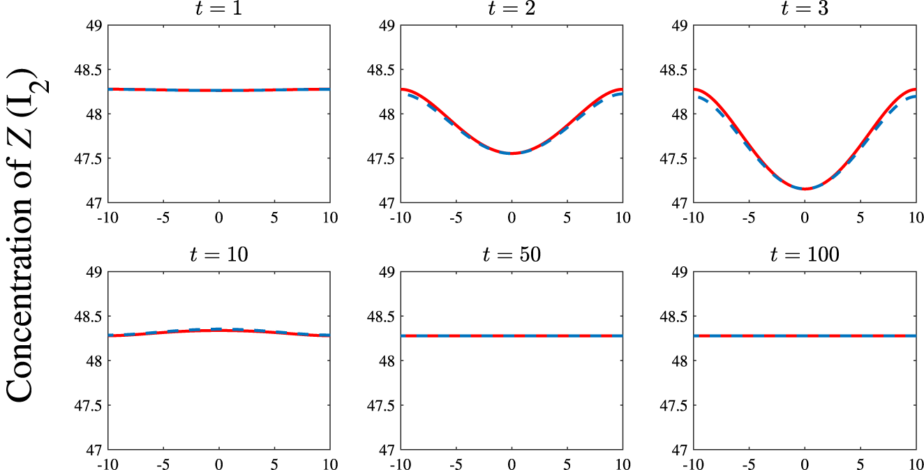
Figure 5 A comparison of the linear (blue, dashed) and nonlinear (red) methods for parameter values $d=0.5$
,
$d=0.5$
, $R_7=0.18$
taken from the stable region of parameter space with the initial condition prescribed in (7.1) with
$R_7=0.18$
taken from the stable region of parameter space with the initial condition prescribed in (7.1) with $M=0.1$
. As expected, after some initial movement away from the steady state the system quickly returns to equilibrium.
$M=0.1$
. As expected, after some initial movement away from the steady state the system quickly returns to equilibrium.
Now we move on to consider parameters taken from the pattern-forming region. In Figure 6 we illustrate the results when $d=0.5$
and
$d=0.5$
and $R_7=0.018$
and for the perturbation amplitude
$R_7=0.018$
and for the perturbation amplitude $M=0.1$
. We would anticipate agreement between the linear and nonlinear solutions for short to intermediate times, and this is observed. On the other hand, we might expect that at longer times the two solutions would deviate from each other; perhaps somewhat surprisingly at
$M=0.1$
. We would anticipate agreement between the linear and nonlinear solutions for short to intermediate times, and this is observed. On the other hand, we might expect that at longer times the two solutions would deviate from each other; perhaps somewhat surprisingly at $t=100$
in Figure 6 this has not yet occurred. However, by
$t=100$
in Figure 6 this has not yet occurred. However, by $t=200$
, significant differences emerge between the two solutions as contributions from higher modes appear in the nonlinear solution.
$t=200$
, significant differences emerge between the two solutions as contributions from higher modes appear in the nonlinear solution.
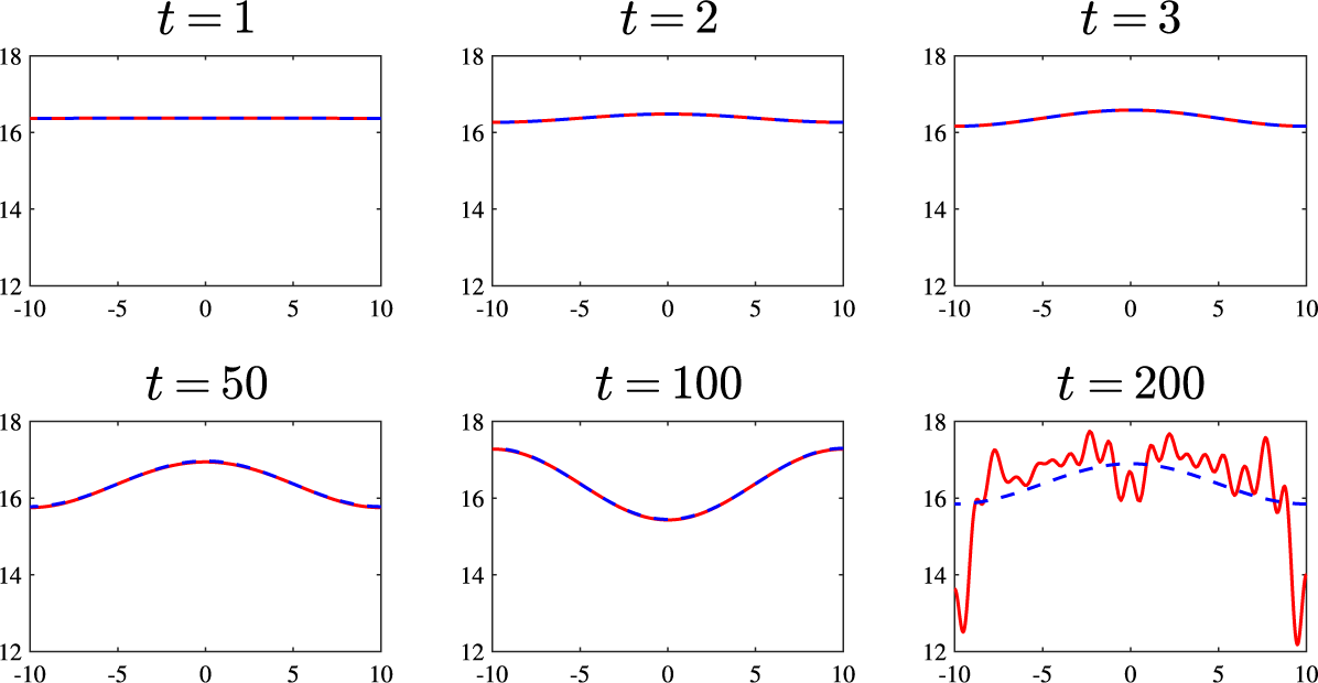
Figure 6 A comparison of the linear (blue, dashed) and nonlinear (red) methods for parameter values $d=0.5$
,
$d=0.5$
, $R_7=0.018$
that lie within the pattern-forming region of parameter space. Amplitude of initial perturbation
$R_7=0.018$
that lie within the pattern-forming region of parameter space. Amplitude of initial perturbation $M=0.1$
.
$M=0.1$
.
As a last example, we conduct another set of simulations with the same parameters used for Figure 6 but now with a substantially larger initial perturbation $M=3$
. With this relatively large deviation from the steady state the linear solution loses validity, rapidly diverging from its nonlinear counterpart. This is confirmed by the results summarized in Figure 7. Here we see the emergence of highly nonlinear patterns from about
$M=3$
. With this relatively large deviation from the steady state the linear solution loses validity, rapidly diverging from its nonlinear counterpart. This is confirmed by the results summarized in Figure 7. Here we see the emergence of highly nonlinear patterns from about $t=10$
onward and a clear difference between linear and nonlinear predictions. After a sufficiently long time the linear solution grows exponentially and includes a region of (physically unrealistic) negative concentrations. By contrast, the nonlinear solution forms flat portions in the concentration profiles, in which the concentrations take on small values, corresponding to the reagents being almost completely depleted in those regions.
$t=10$
onward and a clear difference between linear and nonlinear predictions. After a sufficiently long time the linear solution grows exponentially and includes a region of (physically unrealistic) negative concentrations. By contrast, the nonlinear solution forms flat portions in the concentration profiles, in which the concentrations take on small values, corresponding to the reagents being almost completely depleted in those regions.
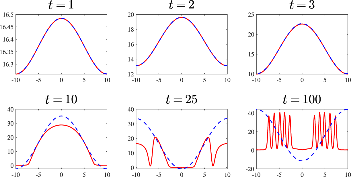
Figure 7 Linear (blue, dashed) and nonlinear (red) results for parameter values $d=0.5$
,
$d=0.5$
, $R_7=0.018$
that lie within the pattern-forming region of parameter space. Amplitude of initial perturbation
$R_7=0.018$
that lie within the pattern-forming region of parameter space. Amplitude of initial perturbation $M=3$
. The increased M is sufficient for the linear and nonlinear results to diverge, with the former becoming unphysical by the time
$M=3$
. The increased M is sufficient for the linear and nonlinear results to diverge, with the former becoming unphysical by the time $t=10$
.
$t=10$
.
7.1 Solutions in other parameter regimes
We noted earlier that the results summarized in Figure 4 can be divided into three distinct zones. Here we turn our attention to the properties of solutions for which the parameters reside in the stable (red) or homogeneous oscillating (purple) parts of parameter space. Within this parameter region the concentration profile becomes spatially homogeneous but the magnitude of this profile oscillates temporally. These classes of solution present some particular challenges inasmuch that there is no straightforward way to visualize the changes that occur over time as they will remain one colour across the entirety of the dish. Perhaps the best way to appreciate the evolution of the reaction is to examine concentration profiles. Once again, we choose $U(x,y,0)=U_{ss}$
, while for Z we take
$U(x,y,0)=U_{ss}$
, while for Z we take
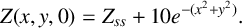 $$ \begin{align} Z(x,y,0) = Z_{ss}+10 e^{-(x^2+y^2)}. \end{align} $$
First, we consider values from the stable region of parameter space ( $d = 0.5, R_7 \,{=}\, 0.18)$
, with the results shown in Figure 8. We see that despite a large initial perturbation the concentration of Z settles to a homogeneous steady state. In passing, we point out that the concentration profiles of U and V are not shown; their development is broadly similar to that of Z with no other features of particular note.
$d = 0.5, R_7 \,{=}\, 0.18)$
, with the results shown in Figure 8. We see that despite a large initial perturbation the concentration of Z settles to a homogeneous steady state. In passing, we point out that the concentration profiles of U and V are not shown; their development is broadly similar to that of Z with no other features of particular note.
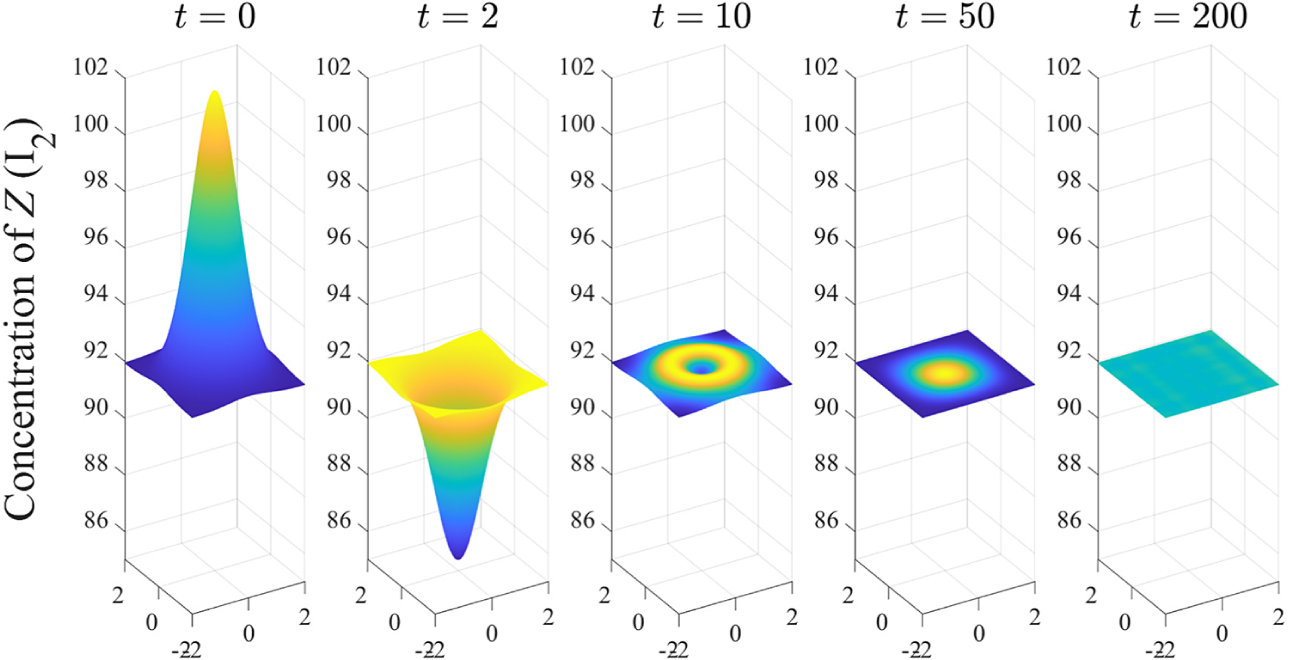
Figure 8 The evolution of the concentration profile of Z ( $\mathrm {I}_2$
) using a large Gaussian perturbation as the initial condition with parameter choices
$\mathrm {I}_2$
) using a large Gaussian perturbation as the initial condition with parameter choices $d=0.5$
and
$d=0.5$
and $R_7=0.18.$
These choices put us in the stable region of parameter space. Consequently, the solution quickly converges to a steady pattern with the value
$R_7=0.18.$
These choices put us in the stable region of parameter space. Consequently, the solution quickly converges to a steady pattern with the value $Z(x,y,t)=Z_{ss}$
.
$Z(x,y,t)=Z_{ss}$
.
Next we consider parameter choices from within the homogeneous oscillations region of parameter space. This terminology warrants some clarification; after some time the concentration across the entire dish tends to a single value which is not constant but rather oscillates in time. To exemplify matters, Figure 9 shows the evolution of the system when $d=0.9$
and
$d=0.9$
and $R_7 = 0.001$
with initial condition (7.2). In the upper panel we see that the system transitions from the initial Gaussian shape to a uniform value across the domain. This value oscillates in time as indicated in the lower panel of Figure 9.
$R_7 = 0.001$
with initial condition (7.2). In the upper panel we see that the system transitions from the initial Gaussian shape to a uniform value across the domain. This value oscillates in time as indicated in the lower panel of Figure 9.
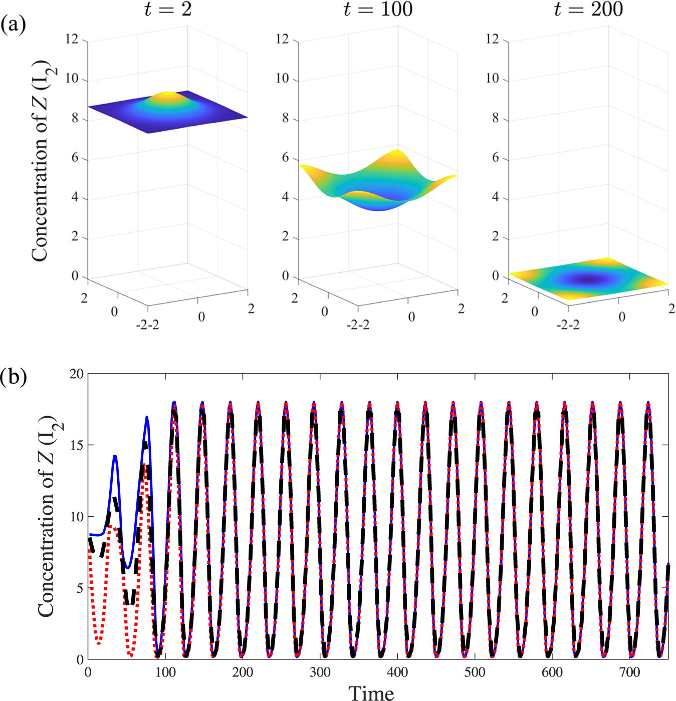
Figure 9 (a) Evolution of the concentration profile of Z ( $\mathrm {I}_2$
) using a Gaussian initial condition and with
$\mathrm {I}_2$
) using a Gaussian initial condition and with $d=0.9$
and
$d=0.9$
and $R_7=0.001$
. The pattern reaches a near homogeneous concentration by the time
$R_7=0.001$
. The pattern reaches a near homogeneous concentration by the time $t=100$
. (b) The homogeneous oscillations in Z at large times. The solid line (blue) marks the maximum of Z across the domain; minimum values are denoted by the dotted line (red). The dashed black line shows the average concentration across the domain as calculated using (7.3). The coincidence of the three lines indicates that the concentration of Z tends to a completely homogeneous value in space.
$t=100$
. (b) The homogeneous oscillations in Z at large times. The solid line (blue) marks the maximum of Z across the domain; minimum values are denoted by the dotted line (red). The dashed black line shows the average concentration across the domain as calculated using (7.3). The coincidence of the three lines indicates that the concentration of Z tends to a completely homogeneous value in space.
We determine the uniform value at a chosen time $t_c$
by calculating the maximum and minimum concentration across the domain when
$t_c$
by calculating the maximum and minimum concentration across the domain when $t=t_c$
. These values are then compared to the average concentration defined to be
$t=t_c$
. These values are then compared to the average concentration defined to be
 $$ \begin{align} Z(t)_{\mathrm{avg}}=\frac{1}{4LB}\int_{-B}^B\int_{-L}^LZ(x,y;t)\,\,dx\,dy. \end{align} $$
After an initial transient we would expect that the profile reaches a spatially homogeneous state that is characterized by maximum, minimum and average concentrations all being the same. This is precisely what is seen in Figure 9(b). It should be noted that this is also what is found if the concentration of V is considered, though in this case the oscillations are reminiscent of a relaxation mechanism rather than the (more sinusoidal) oscillations for Z. It is worth considering what this behaviour would look like in terms of colourized render plots used in Section 5. Taking this viewpoint, the entire dish would spend extended periods appearing blue (indicating that the concentration of V exceeds that of Z). These periods would be punctuated by relatively short bursts during which the entire dish would appear red. Theoretically this cycle would recur indefinitely as long as the supply of reactants is never exhausted.
7.2 Pattern-forming regions
We now investigate the possibilities for the patterns that may form. For all analyses described in this section, we work with the parameter values $d=0.5$
and
$d=0.5$
and $R_7=0.018$
; moreover, unless otherwise stated, we use a domain with
$R_7=0.018$
; moreover, unless otherwise stated, we use a domain with $L=B=2$
. We again use the methods described in Section 5 to visualize our patterns in terms of red and blue hues. A by-product of this work is that we can probe some properties of Turing patterns within this system. In particular, we can confirm that the numbers of minima and maxima in the concentration profiles are functions of the domain size which also dictates the complexity of the pattern that can appear [Reference Murray23].
$L=B=2$
. We again use the methods described in Section 5 to visualize our patterns in terms of red and blue hues. A by-product of this work is that we can probe some properties of Turing patterns within this system. In particular, we can confirm that the numbers of minima and maxima in the concentration profiles are functions of the domain size which also dictates the complexity of the pattern that can appear [Reference Murray23].
Many of these aspects are summarized in Figure 10. The first row demonstrates that when the lengths of the sides of the domain are doubled we change from having approximately four columns of spots to eight. In the bottom row of Figure 10 the width of the box has been markedly reduced and the domain is so narrow that the wavelength of the largest positive eigenvalue is greater than B. Turing theory then predicts that patterns cannot form in the y-direction, and this is confirmed by the appearance of stripes along the length of the box.
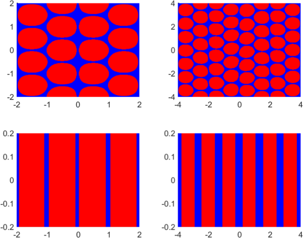
Figure 10 A demonstration of how Turing patterns change with the size of the domain. In the first row, we use a box with an aspect ratio of $1$
and parameter values
$1$
and parameter values $d=0.5$
and
$d=0.5$
and $R_7=0.018$
. Left
$R_7=0.018$
. Left $L=B=2$
, right
$L=B=2$
, right $L=B=4$
. In the bottom row we consider narrow boxes with a fixed width
$L=B=4$
. In the bottom row we consider narrow boxes with a fixed width $B=0.2$
. Left
$B=0.2$
. Left $L=2$
, right
$L=2$
, right $L=4$
.
$L=4$
.
We observe, too, that stripes are not only possible in narrow boxes. Indeed, stripes can even appear within a square box if the initial conditions are chosen to be varying in only one direction such as those used in Figures 11(c) and 13. All the patterns illustrated in Figure 10 were generated from the initial condition
 $$ \begin{align*}G(x,y) =Z_{ss}+ \cos\bigg(\frac{\pi (x+L)}{2L}\bigg)+0.6\bigg[\cos\bigg(\frac{2\pi (x+L)}{2L}\bigg)+\cos\bigg(\frac{\pi (y+B)}{2B}\bigg)\bigg],\end{align*} $$
which helps support the idea that the formation of striped patterns is a direct consequence of reducing the width of the box. This phenomenon is confirmation of the well-known result that the patterning becomes structurally simpler as the aspect ratio grows [Reference Murray23]. A well-known example of this effect can be observed in the coats of many animals of the feline family such as cats and cheetahs, where colour variations are spots on the body, but stripes on the narrower tails [Reference Murray23].
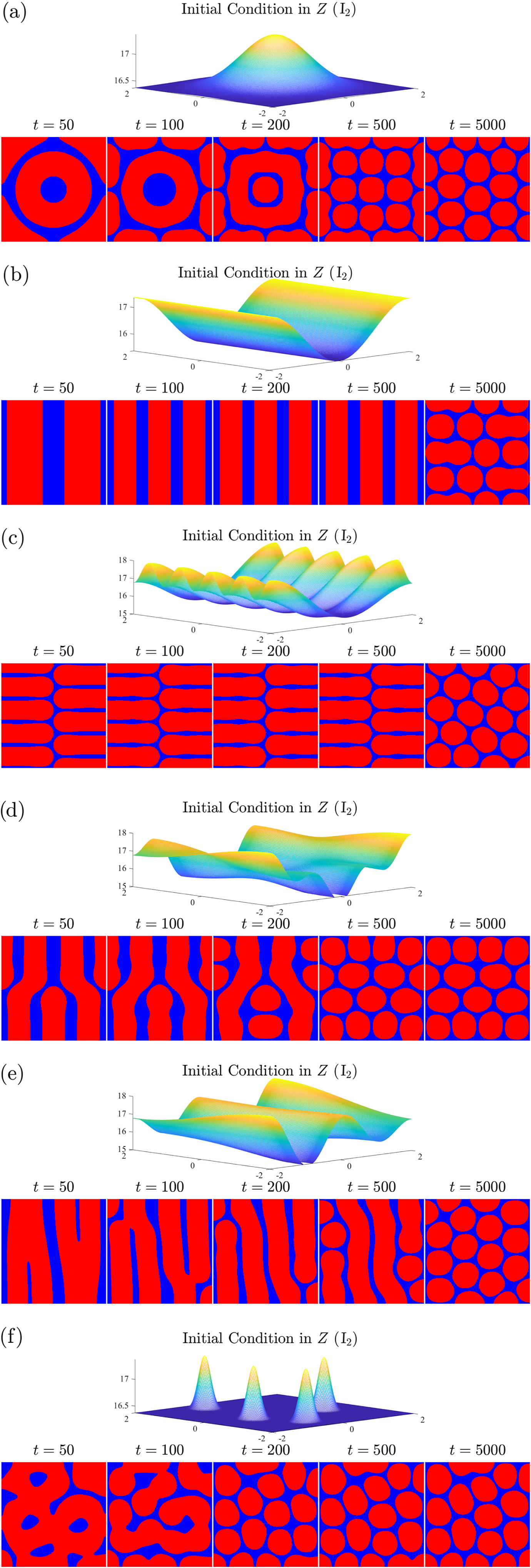
Figure 11 Six examples of the evolution of patterns in a box with dimensions $(x,\,y)\in (-2,\,2)$
. In each instance we show the initial concentration profile of Z with U beginning at its steady-state value. Following this, we show how the patterns evolve with time. (a) The Gaussian initial profile (7.4). (b) The cosine initial condition (7.5). In the next three cases we have used perturbed conditions of the type (7.6). In (c)
$(x,\,y)\in (-2,\,2)$
. In each instance we show the initial concentration profile of Z with U beginning at its steady-state value. Following this, we show how the patterns evolve with time. (a) The Gaussian initial profile (7.4). (b) The cosine initial condition (7.5). In the next three cases we have used perturbed conditions of the type (7.6). In (c) $\gamma =1,\,\beta _1=1 $
and
$\gamma =1,\,\beta _1=1 $
and $\beta _2=9$
; in (d)
$\beta _2=9$
; in (d) $\gamma =2$
,
$\gamma =2$
, $\beta _1=6$
and
$\beta _1=6$
and $\beta _2=1$
; and in (e)
$\beta _2=1$
; and in (e) $\gamma =4$
,
$\gamma =4$
, $\beta _1=3$
and
$\beta _1=3$
and $\beta _2=1$
. Finally, in (f) the initial condition consists of four random spikes each of Gaussian form.
$\beta _2=1$
. Finally, in (f) the initial condition consists of four random spikes each of Gaussian form.
In Figure 11 we show a selection of patterns that evolve starting from various initial conditions and using $71\times 71$
Fourier modes. Figure 11(a) illustrates the results if we begin with the Gaussian profile
$71\times 71$
Fourier modes. Figure 11(a) illustrates the results if we begin with the Gaussian profile
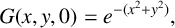 $$ \begin{align} G(x,y,0)=e^{- (x^2+y^2)}, \end{align} $$
while for Figure 11(b) we have adopted the primary mode
 $$ \begin{align} G(x,y,0)=\cos\bigg(\frac{\pi(x+L)}{2L}\bigg). \end{align} $$
The next three examples illustrate various perturbed mode distributions
 $$ \begin{align} G(x,y,0)= \cos\bigg(\gamma\frac{\pi(x+L)}{2L}\bigg)+ 0.6\bigg[\cos\bigg(\beta_1\frac{\pi(x+L)}{2L}\bigg)+ \cos\bigg(\beta_2\frac{\pi(y+B)}{2B}\bigg)\bigg] \end{align} $$
with the adventurers $\alpha ,\,\beta _1$
and
$\alpha ,\,\beta _1$
and $\beta _2$
specified in the caption of Figure 11. Finally, we present a case where we have four “random” spikes each of which is Gaussian in shape. We imagine this example as what may happen if four drops of iodine are added to an otherwise homogeneous distribution.
$\beta _2$
specified in the caption of Figure 11. Finally, we present a case where we have four “random” spikes each of which is Gaussian in shape. We imagine this example as what may happen if four drops of iodine are added to an otherwise homogeneous distribution.
We make particular note of the results from Figures 11(b) and (c). In these images we observe that the pattern seems to have attained a steady-state configuration at relatively early times ( $t=100$
). However, it becomes apparent that these patterns are still evolving and eventually they develop a very different structure. This sequence of events is most evident in (b) and (c) where the pattern changes significantly between
$t=100$
). However, it becomes apparent that these patterns are still evolving and eventually they develop a very different structure. This sequence of events is most evident in (b) and (c) where the pattern changes significantly between $t=500$
and
$t=500$
and $t=5000$
.
$t=5000$
.
We propose that the delayed switching in patterns is due to different reasons. When we begin with a unidirectional initial condition (one with perturbations in only one direction) such as in (b) the change in pattern from stripes to spots can be attributed to a compounding of numerical inaccuracies that is built up over time and which cause slight perturbations to the steady pattern. Evidence that these are numerical errors is obtained from noting that the transition to the new steady state can be postponed (but not prevented) by increasing the accuracy of the numerical integration. This is in accord with the behaviour we saw with circular patterns in Section 5, where a small perturbation could lead to a transition to a new steady pattern. We provide an example of this in Figure 12. In this figure, we present two sets of results, one with $51\times 51$
modes and high error tolerances (relative error tolerance
$51\times 51$
modes and high error tolerances (relative error tolerance $=10^{-3}$
, absolute error tolerance
$=10^{-3}$
, absolute error tolerance $=10^{-5}$
) and another which uses
$=10^{-5}$
) and another which uses $71\times 71$
modes with very low error tolerances (relative error tolerance
$71\times 71$
modes with very low error tolerances (relative error tolerance $=10^{-10}$
, absolute error tolerance
$=10^{-10}$
, absolute error tolerance $=10^{-12}$
). In Figure 12(a) the first indications of numerical error can be seen by
$=10^{-12}$
). In Figure 12(a) the first indications of numerical error can be seen by $t=3000$
and the pattern no longer resembles stripes by
$t=3000$
and the pattern no longer resembles stripes by $t=3600$
, whereas in the higher-accuracy Figure 12(b) the accumulation of numerical inaccuracies is only beginning at
$t=3600$
, whereas in the higher-accuracy Figure 12(b) the accumulation of numerical inaccuracies is only beginning at $t=3600$
. Both Figures 12(a) and 12(b) ultimately settled to the same spotted pattern (although interestingly it is vertically shifted). It appears that this is a genuine final state of the system as it did not change even when we computed to very long times
$t=3600$
. Both Figures 12(a) and 12(b) ultimately settled to the same spotted pattern (although interestingly it is vertically shifted). It appears that this is a genuine final state of the system as it did not change even when we computed to very long times $t\approx 30\,000$
. This reinforces our belief that there is a plethora of possible steady patterns, some of which are intrinsically more stable than others. For instance, it seems that a striped pattern, while persisting for some duration, will eventually evolve to a more stable spotted structure. We point out that this phenomenon of transition between patterns may not be unrealistic. In a laboratory setting it is quite conceivable that an experiment could reach one steady pattern and then, if the dish is nudged or otherwise perturbed, this could be sufficient to cause the pattern to transition to another, more stable, configuration.
$t\approx 30\,000$
. This reinforces our belief that there is a plethora of possible steady patterns, some of which are intrinsically more stable than others. For instance, it seems that a striped pattern, while persisting for some duration, will eventually evolve to a more stable spotted structure. We point out that this phenomenon of transition between patterns may not be unrealistic. In a laboratory setting it is quite conceivable that an experiment could reach one steady pattern and then, if the dish is nudged or otherwise perturbed, this could be sufficient to cause the pattern to transition to another, more stable, configuration.
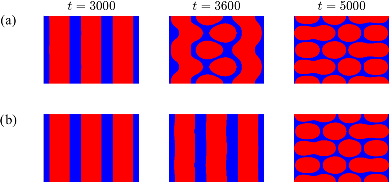
Figure 12 Evolution of spatial patterns in a box of dimensions $x,y\in (-2,2)$
using the initial condition (7.5). In (a) we use a spectral method using
$x,y\in (-2,2)$
using the initial condition (7.5). In (a) we use a spectral method using $51\times 51$
modes with relative error tolerance
$51\times 51$
modes with relative error tolerance $=10^{-3}$
, absolute error tolerance
$=10^{-3}$
, absolute error tolerance $=10^{-5}$
and in (b) we use a spectral method using
$=10^{-5}$
and in (b) we use a spectral method using $71\times 71$
modes with very low error tolerances (relative error tolerance
$71\times 71$
modes with very low error tolerances (relative error tolerance $=10^{-10}$
and absolute error tolerance
$=10^{-10}$
and absolute error tolerance $=10^{-12}$
). By comparing the two methods we see that the numerical error begins to become present earlier in the lower-precision computation, leading to the presence of spots.
$=10^{-12}$
). By comparing the two methods we see that the numerical error begins to become present earlier in the lower-precision computation, leading to the presence of spots.
It is of some interest to ask whether within many various patterns there are some that are distinctly preferred over others. To address this question we undertook an extensive investigation consisting of 729 individual cases. In these we considered various initial conditions from (7.6) where the positive integers $\gamma $
,
$\gamma $
, $\beta _1$
and
$\beta _1$
and $\beta _2$
satisfy
$\beta _2$
satisfy $1\leq \gamma ,\beta _1, \beta _2\leq 9$
. Each simulation was extended to
$1\leq \gamma ,\beta _1, \beta _2\leq 9$
. Each simulation was extended to $t=10\,000$
to ensure that the correct final steady pattern had been reached. The results confirmed our suspicion that a range of stable patterns are possible. The majority of these possess a spot-like character, most of which are arranged in an approximately
$t=10\,000$
to ensure that the correct final steady pattern had been reached. The results confirmed our suspicion that a range of stable patterns are possible. The majority of these possess a spot-like character, most of which are arranged in an approximately $4\times 4$
configuration. Other configurations appeared as straight lines; these always had four stripes, reminiscent of the form shown in the final plot of the penultimate column of Figure 11(b). Finally, there was a small subset of patterns that were different again. The conclusion is that the spot-like patterns seem to be the most stable ones and thus are perhaps the most likely to be seen in practice. This conclusion is supported by the work of Ermentrout [Reference Ermentrout13] who showed that the presence of quadratic nonlinear terms tends to lead to the formation of spots as the dominant pattern. Therefore, for our model for all pattern-forming parameter values where a genuinely two-dimensional initial condition is given, a spotted pattern is anticipated.
$4\times 4$
configuration. Other configurations appeared as straight lines; these always had four stripes, reminiscent of the form shown in the final plot of the penultimate column of Figure 11(b). Finally, there was a small subset of patterns that were different again. The conclusion is that the spot-like patterns seem to be the most stable ones and thus are perhaps the most likely to be seen in practice. This conclusion is supported by the work of Ermentrout [Reference Ermentrout13] who showed that the presence of quadratic nonlinear terms tends to lead to the formation of spots as the dominant pattern. Therefore, for our model for all pattern-forming parameter values where a genuinely two-dimensional initial condition is given, a spotted pattern is anticipated.
7.3 The effect of diffusion on pattern formation
We have already noted that the results to date have been obtained with a dimensional diffusion coefficient of $2.75\times 10^{-6}\,\mathrm {m}^2\mathrm {s}^{-1}$
. This choice, combined with a suitable lengthscale, enabled us to consider dimensionless diffusion coefficients around
$2.75\times 10^{-6}\,\mathrm {m}^2\mathrm {s}^{-1}$
. This choice, combined with a suitable lengthscale, enabled us to consider dimensionless diffusion coefficients around $10^{-2}$
. Typical dimensional diffusion coefficients for fluids in water are of the order of
$10^{-2}$
. Typical dimensional diffusion coefficients for fluids in water are of the order of $10^{-9}\, \mathrm {m}^2\mathrm {s}^{-1}$
which would translate to dimensionless values of around
$10^{-9}\, \mathrm {m}^2\mathrm {s}^{-1}$
which would translate to dimensionless values of around $10^{-5}$
, found to be too computationally demanding even on a high-performance computer with a fast GPU. As our initial condition relies on the mixing of two fluids we posited that it may have been, in part, a viscous mixing process. This is plausible since the kinematic viscosity of water is roughly
$10^{-5}$
, found to be too computationally demanding even on a high-performance computer with a fast GPU. As our initial condition relies on the mixing of two fluids we posited that it may have been, in part, a viscous mixing process. This is plausible since the kinematic viscosity of water is roughly $10^{-6}\, \mathrm {m}^2\mathrm {s}^{-1}$
. We now discuss how our patterns change as we decrease our diffusion coefficient to a more sensible value, thereby modelling how results might change should the underlying driving physics change from that of a viscous process towards a true diffusion action.
$10^{-6}\, \mathrm {m}^2\mathrm {s}^{-1}$
. We now discuss how our patterns change as we decrease our diffusion coefficient to a more sensible value, thereby modelling how results might change should the underlying driving physics change from that of a viscous process towards a true diffusion action.
In Figure 13 we show the effect of reducing the dimensionless diffusion $D_z$
from
$D_z$
from $10^{-2}$
to
$10^{-2}$
to $10^{-4}$
; this range corresponds to dimensional values between
$10^{-4}$
; this range corresponds to dimensional values between $2.75\times 10^{-6}$
and
$2.75\times 10^{-6}$
and $2.75\times 10^{-8}\,\mathrm {m}^2\mathrm {s}^{-1}$
. While this might not quite capture the range of a true diffusion coefficient, it does show a clear trend. As the diffusion coefficient falls, so the number of stripes increases. When
$2.75\times 10^{-8}\,\mathrm {m}^2\mathrm {s}^{-1}$
. While this might not quite capture the range of a true diffusion coefficient, it does show a clear trend. As the diffusion coefficient falls, so the number of stripes increases. When $D_z$
was reduced to around
$D_z$
was reduced to around $10^{-4}$
the tendency to form dots rather than stripes is strong enough that even though the initial condition had no component in the y-direction, machine precision variations are enough to seed the y-variability seen in the rightmost panel. This is the case even if as many as
$10^{-4}$
the tendency to form dots rather than stripes is strong enough that even though the initial condition had no component in the y-direction, machine precision variations are enough to seed the y-variability seen in the rightmost panel. This is the case even if as many as $256^2$
Fourier modes were used. We point out that the patterns in Figure 13 were obtained from an initial condition which only varies in x while y is held constant. By doing this we force the system to start with a one-dimensional structure which restricts the possible final outcomes.
$256^2$
Fourier modes were used. We point out that the patterns in Figure 13 were obtained from an initial condition which only varies in x while y is held constant. By doing this we force the system to start with a one-dimensional structure which restricts the possible final outcomes.
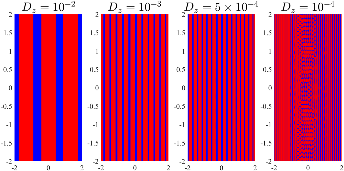
Figure 13 The patterns that form at $t=1000$
for a range of values
$t=1000$
for a range of values $D_z$
; all the other parameters and initial condition remain unaltered. The initial condition was constant in y with one cosine wave in the x-direction.
$D_z$
; all the other parameters and initial condition remain unaltered. The initial condition was constant in y with one cosine wave in the x-direction.
It is clear from Figure 13 that the number of stripes is related to the diffusion coefficient. This dependence can be explained by reference to the linearized system described in Section 6.1. If k denotes the wavenumber of the solution, the eigenvalues of the linearized system are
 $$ \begin{align*}\lambda^\pm = \tfrac{1}{2}\Big [(f_u+g_z)-k^2(D_u+D_z)\pm \sqrt{(k^2(D_z-D_u)+f_u-g_z)^2+4f_zg_u}\, \Big],\end{align*} $$
where $f_u=S_1,\, f_z=S_2$
as defined in (4.2) and evaluated at
$f_u=S_1,\, f_z=S_2$
as defined in (4.2) and evaluated at $(U_{ss},\,Z_{ss})$
,
$(U_{ss},\,Z_{ss})$
, $g_u=R_3$
and
$g_u=R_3$
and ${g_z=-\alpha }$
.
${g_z=-\alpha }$
.
Ultimately, we wish to understand how the dominant mode of the pattern varies with the size of $D_z$
. If we regard the eigenvalue
$D_z$
. If we regard the eigenvalue $\lambda \equiv \lambda (T)$
where
$\lambda \equiv \lambda (T)$
where $T\equiv k^2$
, then
$T\equiv k^2$
, then
 $$ \begin{align*}\lambda (T) =\tfrac{1}{2}\Big [(f_u+g_z)-T(D_u+D_z)+ \sqrt{(T(D_z-D_u)+f_u-g_z)^2+4f_zg_u}\,\Big]. \end{align*} $$
Of importance is the greatest value of $\lambda $
as k varies, since this sets the lengthscale of the fastest-growing mode. If we put
$\lambda $
as k varies, since this sets the lengthscale of the fastest-growing mode. If we put
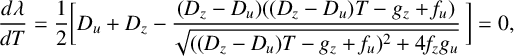 $$ \begin{align*}\frac{d\lambda}{dT}=\frac{1}{2}\bigg[D_u+D_z-\frac{(D_z-D_u)((D_z-D_u)T-g_z+f_u)}{\sqrt{((D_z-D_u)T-g_z+f_u)^2+4f_zg_u}}\,\bigg]=0,\end{align*} $$
we obtain the quadratic
 $$ \begin{align*}\{ A^2(A^2-B^2) \} T^2+\{ 2AC(A^2-B^2)\}T+C^2(A^2-B^2)-4B^2f_zg_u=0;\end{align*} $$
here we have defined the constants
 $$ \begin{align*}A\equiv D_z-D_u=D_z(1-d),\quad B\equiv D_z+D_u=D_z(1+d)\quad\mathrm{and}\quad C\equiv f_u-g_z.\end{align*} $$
The solution corresponding to the largest eigenvalue is
 $$ \begin{align*}T=k^2=\frac{1}{D_z(1-d)}\bigg[g_z-f_u+\sqrt{\frac{f_zg_u}{d}}\,\bigg],\end{align*} $$
which shows that the most influential mode of the linearized system has a wavenumber proportional to $1/\sqrt {D_z}$
. Since
$1/\sqrt {D_z}$
. Since $D_z$
is defined as
$D_z$
is defined as
 $$ \begin{align*}D_z\equiv\frac{\sigma_x T_s}{L_s^2},\end{align*} $$
reducing the dimensionless diffusion coefficient by a given factor can be achieved in two ways: either by decreasing the dimensional diffusion coefficient by the same factor, or by increasing the characteristic lengthscale by the square root of that factor. It follows that the predicted pattern wavelength is $\lambda _{\mathrm {wl}} = {2\pi }/{\sqrt {T}}$
and that the number of stripes across the domain would be
$\lambda _{\mathrm {wl}} = {2\pi }/{\sqrt {T}}$
and that the number of stripes across the domain would be
 $$ \begin{align} P_{x} = \frac{2L}{\lambda_{\mathrm{wl}}}. \end{align} $$
In Figure 14 we summarize this relationship between fastest-growing mode and diffusion. Five points on this curve have been highlighted and the numbers of patterns that can fit within the domain $x\in [-2,\,2]$
are indicated. The numbers of patterns are respectively 111 (at which the dimensional diffusion coefficient is
$x\in [-2,\,2]$
are indicated. The numbers of patterns are respectively 111 (at which the dimensional diffusion coefficient is $\sigma _z\,{=}\,2.75\times 10^{-9}\,\mathrm {m}^2\mathrm {s}^{-1}$
), 35 (
$\sigma _z\,{=}\,2.75\times 10^{-9}\,\mathrm {m}^2\mathrm {s}^{-1}$
), 35 ( $\sigma _z=2.75\times 10^{-8}\,\mathrm {m}^2\mathrm {s}^{-1}$
), 15 (
$\sigma _z=2.75\times 10^{-8}\,\mathrm {m}^2\mathrm {s}^{-1}$
), 15 ( $\sigma _z=5\times 10^{-4}\,\mathrm {m}^2\mathrm {s}^{-1}$
), 11 (
$\sigma _z=5\times 10^{-4}\,\mathrm {m}^2\mathrm {s}^{-1}$
), 11 ( $\sigma _z=2.75\times 10^{-7}\,\mathrm {m}^2\mathrm {s}^{-1}$
) and 3.5 (
$\sigma _z=2.75\times 10^{-7}\,\mathrm {m}^2\mathrm {s}^{-1}$
) and 3.5 ( $\sigma _z=2.75\times 10^{-6}\,\mathrm {m}^2\mathrm {s}^{-1}$
). When we compare the results of this prediction to the numerical results shown in Figure 13, we find that the linearized method does a commendable job in predicting how many stripes will be seen for a given diffusion coefficient such that in each case the linear prediction is within one stripe of what is shown in Figure 13. It is important to clarify that this is, of course, only valid in the pattern-forming region of parameter space where the maximal eigenvalue is greater than zero.
$\sigma _z=2.75\times 10^{-6}\,\mathrm {m}^2\mathrm {s}^{-1}$
). When we compare the results of this prediction to the numerical results shown in Figure 13, we find that the linearized method does a commendable job in predicting how many stripes will be seen for a given diffusion coefficient such that in each case the linear prediction is within one stripe of what is shown in Figure 13. It is important to clarify that this is, of course, only valid in the pattern-forming region of parameter space where the maximal eigenvalue is greater than zero.
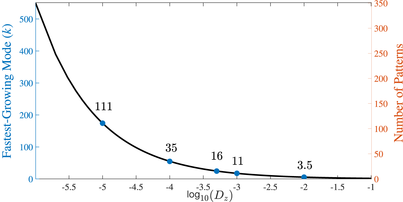
Figure 14 The wavenumber of the fastest-growing mode as a function of the diffusion coefficient. We also indicate the corresponding number of stripes observed based upon equation (7.7) on the orange, right-hand-side y-axis. We highlight some particular points and explicitly state how many patterns would be expected in the x-direction.
Therefore, if these patterns could be visualized experimentally, in a dish of this shape ( $20\times 20~\mathrm {cm}$
) and assuming
$20\times 20~\mathrm {cm}$
) and assuming $\sigma _z=2.75\times 10^{-9}~ \mathrm {m}^2\mathrm {s}^{-1}$
, we would expect to see stripes or spots forming with a wavelength of approximately
$\sigma _z=2.75\times 10^{-9}~ \mathrm {m}^2\mathrm {s}^{-1}$
, we would expect to see stripes or spots forming with a wavelength of approximately $2\,\mathrm {mm}$
. Convergence to a steady pattern would be expected within a number of hours, with the exact amount of time dependent on the initial condition. This assumes that the presence of oxygen does not disrupt the formation of bubbles.
$2\,\mathrm {mm}$
. Convergence to a steady pattern would be expected within a number of hours, with the exact amount of time dependent on the initial condition. This assumes that the presence of oxygen does not disrupt the formation of bubbles.
8 Concluding remarks
In this work, we have developed a spatially extended model of the Bray–Liebhafsky chemical reaction. On one level the model is quite simple, but it retains sufficient structure to enable spatial pattern formation. We have calculated both one-dimensional, axisymmetric target patterns in a circular beaker as well as two-dimensional configurations that may occur in a rectangular reaction vessel. We have uncovered a wide range of possible patterns; which is actually seen in any practical setting is a function of the particular initial conditions at hand. Most structures appear as either spots or stripes. As our formulation was derived based on realistic practical values, we speculate that the Bray–Liebhafsky system exhibits kinetic behaviour consistent with the formation of spatial patterns. A further direction for the mathematical model of this reaction is to look at a slowly growing domain to see if the patterns that are formed eventually evolve into spots. As the characteristic wavelength of the patterns would be expected to stay the same, we may see phenomena such as spot-splitting as discussed in Crampin et al. [Reference Crampin, Gaffney and Main8].
While we have been able to uncover some characteristic linear and nonlinear solutions using both one- and two-dimensional geometries, what is presently lacking is any complementary experimental work. We have previously alluded to the fact that it appears that little practical work has been conducted in relation to the Bray–Liebhafsky reaction; this can be ascribed to the absence of visually observable patterns. It is possible that an experimental investigation in the UV frequency range may allow laboratory visualization for the spatial patterns, in which case target patterns similar to Figure 3 might be anticipated. In addition, more complicated nonaxisymmetric configurations, such as scroll waves, may prove feasible in circular domains. Such structures could be found by generalizing the Fourier–Bessel formulation (5.1) adopted in Section 5; such an extension would require substantial additional computational power and is left for future investigation.
Acknowledgments
This work constitutes part of a project conducted by the first author during his Honours year (2023) and first year of his PhD (2024) at the University of Tasmania. He thanks the trustees of the Forbes and Warren scholarship for support through his Honours studies. Support from the Australian Government Research Training Program Scholarship is also gratefully acknowledged. We are also very grateful to the two anonymous reviewers for their detailed and insightful suggestions.
Appendix A Implementation of the method of lines
Here we outline the process used to apply the method of lines to our two-dimensional system. This method of lines is a finite-difference method whereby every dimension except one is discretized, which turns the system of equations into a system of semi-discretized ordinary differential equations. This technique is particularly useful for integrating systems involving simple geometries such as the rectangles used here. For more complex geometries it may be appropriate to employ a more sophisticated procedure such as the finite-element method.
Here, we will apply a standard second-order accurate finite-difference method for a second-order equation. To begin, we discretized our spatial domains and suppose that time is a continuous variable. We start by forming a regularly spaced $(m+1)\times (n+1)$
grid in which meshpoints in the x-direction are located at
$(m+1)\times (n+1)$
grid in which meshpoints in the x-direction are located at $-L=x_0,\,x_1,\ldots ,x_{m-1}$
and
$-L=x_0,\,x_1,\ldots ,x_{m-1}$
and $x_m=L$
, while in the y-direction we have
$x_m=L$
, while in the y-direction we have $-B=y_0, y_1,\ldots ,y_{n-1}$
and
$-B=y_0, y_1,\ldots ,y_{n-1}$
and $y_n=B$
.
$y_n=B$
.
Next we discretize the governing equations (6.2), and we cast the Laplacian as
 $$ \begin{align*} \nabla^2\phi_{i,j}=\frac{\phi_{i+1,j}(t)-2\phi_{i,j}(t)+\phi_{i-1,j}(t)}{\Delta x^2}+\frac{\phi_{i,j+1}(t)-2\phi_{i,j}(t)+\phi_{i,j-1}(t)}{\Delta y^2}, \end{align*} $$
where $\phi $
represents our concentration variables, either U or Z. Furthermore,
$\phi $
represents our concentration variables, either U or Z. Furthermore, ${i =0, 1,\ldots ,m }$
,
${i =0, 1,\ldots ,m }$
, $j=0,1,\ldots ,n$
,
$j=0,1,\ldots ,n$
, $\Delta x=x_i-x_{i-1}$
and
$\Delta x=x_i-x_{i-1}$
and $\Delta y=y_j-y_{j-1}.$
Our finite-difference method representation of the Laplacian cannot be used at the boundaries as it requires knowledge of $x_{-1},\,x_{m+1},\, y_{-1}$
and
$x_{-1},\,x_{m+1},\, y_{-1}$
and $y_{n+1}$
which lie outside the computational region. We circumvent this difficulty by appealing to our reflective (Neumann) boundary conditions that allow us to create “false boundaries”. In this way we conclude that
$y_{n+1}$
which lie outside the computational region. We circumvent this difficulty by appealing to our reflective (Neumann) boundary conditions that allow us to create “false boundaries”. In this way we conclude that $U_{-1,j}=U_{1,j}$
,
$U_{-1,j}=U_{1,j}$
, $U_{m+1,j}=U_{m-1,j}$
,
$U_{m+1,j}=U_{m-1,j}$
, $U_{i,-1}=U_{i,1}$
and
$U_{i,-1}=U_{i,1}$
and $U_{i,j+1}=U_{i,j-1}$
with equivalent results for Z.
$U_{i,j+1}=U_{i,j-1}$
with equivalent results for Z.
Our system of semi-discretized equations becomes
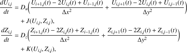 $$ \begin{align*} \frac{d U_{i,j}}{d t} &= D_u\bigg(\frac{U_{i+1,j}(t)-2U_{i,j}(t)+U_{i-1,j}(t)}{\Delta x^2} +\frac{U_{i,j+1}(t)-2U_{i,j}(t)+U_{i,j-1}(t)}{\Delta y^2}\bigg) \\ &\quad +J(U_{i,j},Z_{i,j}), \\ \frac{d Z_{i,j}}{d t}& = D_z\bigg(\frac{Z_{i+1,j}(t)-2Z_{i,j}(t)+Z_{i-1,j}(t)}{\Delta x^2} +\frac{Z_{i,j+1}(t)-2Z_{i,j}(t)+Z_{i,j-1}(t)}{\Delta y^2}\bigg) \\&\quad +K(U_{i,j},Z_{i,j}), \end{align*} $$
in which we have defined
 $$ \begin{align*} J(U_{i,j},Z_{i,j})& \equiv R_3U_{i,j} + \frac{R_1-U_{i,j}}{R_1+U_{i,j}}Z_{i,j}-R_4U_{i,j}^2 , \\[6pt]K(U_{i,j},Z_{i,j}) &\equiv R_3U_{i,j}-\alpha Z_{i,j}.\end{align*} $$
Now that we have our equations for each point in the grid we can solve them numerically. To do this, we used the ode45 package within MATLAB to integrate the system forwards in time. When the script was written using exclusively matrix multiplication, we were able to produce results in similar times to those using the spectral method. However, when trying to yield highly accurate results (requiring $>250$
meshpoints) the spectral method was much more efficient than this second-order method.
$>250$
meshpoints) the spectral method was much more efficient than this second-order method.


 Open access