


1 Introduction
In this article, we are concerned with the following parabolic equation involving tempered fractional operator:
 $$ \begin{align} \frac{\partial u}{\partial t}(x, t)-\left(\Delta+\lambda\right)^{\frac{\alpha}{2}} u(x, t)=f(u(x, t)), \end{align} $$
where the tempered fractional Laplacian operator $-\left (\Delta +\lambda \right )^{\frac {\alpha }{2}}$
is defined as
$-\left (\Delta +\lambda \right )^{\frac {\alpha }{2}}$
is defined as
 $$ \begin{align} \left(\Delta+\lambda\right)^{\frac{\alpha}{2}}u(x,t):=-c_{n,\alpha} P.V. \int_{\mathbb{R}^{n}} \frac{u(x,t)-u(y,t)}{e^{\lambda|x-y|}|x-y|^{{n+\alpha}}}d y, \end{align} $$
where $P.V.$
stands for Cauchy principal value, and
$P.V.$
stands for Cauchy principal value, and
 $$ \begin{align} c_{n,\alpha}=\left\{{\begin{array}{@{}l} {\frac{\alpha\Gamma(\frac{n+\alpha}{2})}{2^{1-\alpha}\pi^{\frac{n}{2}}|\Gamma(1-\frac{\alpha}{2})|},\quad \text{for}\,\,\lambda=0\,\,\text{or}\,\,\alpha=1,} \\ {} \\ {\frac{\Gamma(\frac{n}{2})}{2\pi^{\frac{n}{2}}|\Gamma(-\alpha)|}, \quad \text{for}\,\,\lambda>0\,\,\text{and}\,\,\alpha\neq1,} \\ \end{array}} \right. \end{align} $$
and $\Gamma $
denotes the Gamma function.
$\Gamma $
denotes the Gamma function.
To ensure that the right-hand side of the definition (1.3) is well-defined, we require that $u(x,t) \in \{\mathscr {L}_{\alpha }(\mathbb {R}^{n})\cap C_{\text {loc }}^{1,1}(\mathbb {R}^{n}\setminus \{0\})\}\times C^{1}(\mathbb R)$
with
$u(x,t) \in \{\mathscr {L}_{\alpha }(\mathbb {R}^{n})\cap C_{\text {loc }}^{1,1}(\mathbb {R}^{n}\setminus \{0\})\}\times C^{1}(\mathbb R)$
with
 $$ \begin{align} \mathscr{L}_{\alpha}(\mathbb{R}^{n}):=\left\{u(\cdot,t)\in L_{loc}^{1}(\mathbb R^n) \,\Bigg|\, \int_{\mathbb{R}^{n}} \frac{e^{-\lambda|x|}|u(x,t)|}{1+|x|^{n+\alpha}}dx<+\infty\right\}. \end{align} $$
Throughout this article, we say that u is an classical entire solution of problem (1.1) if
 $$ \begin{align*}u(x,t) \in \{\mathscr{L}_{\alpha}(\mathbb{R}^{n})\cap C_{\text {loc }}^{1,1}(\mathbb{R}^{n}\setminus \{0\})\}\times C^{1}(\mathbb R). \end{align*} $$
When $\lambda \rightarrow 0+$
, the tempered fractional operator
$\lambda \rightarrow 0+$
, the tempered fractional operator $-\left (\Delta +\lambda \right )^{\frac {\alpha }{2}}$
degenerate into the familiar fractional Laplacian
$-\left (\Delta +\lambda \right )^{\frac {\alpha }{2}}$
degenerate into the familiar fractional Laplacian $(-\Delta )^{\frac {\alpha }{2}}$
, which is also a nonlocal integro-differential operator given by
$(-\Delta )^{\frac {\alpha }{2}}$
, which is also a nonlocal integro-differential operator given by
 $$ \begin{align} (-\Delta)^{\frac{\alpha}{2}} u(x,t) = C_{n,\alpha} \, P.V. \int_{\mathbb{R}^N} \frac{u(x,t)-u(y,t)}{|x-y|^{N+\alpha}} dy, \end{align} $$
where $0<\alpha <2$
,
$0<\alpha <2$
, $\displaystyle C_{n,\alpha }=(\int _{\mathbb R^{n}}{\frac {1-\cos (2\pi y_{1})}{|y|^{n+\alpha }}dy})^{-1}$
. Fractional Laplacian
$\displaystyle C_{n,\alpha }=(\int _{\mathbb R^{n}}{\frac {1-\cos (2\pi y_{1})}{|y|^{n+\alpha }}dy})^{-1}$
. Fractional Laplacian $(-\Delta )^{\frac {\alpha }{2}} $
is well-defined for any
$(-\Delta )^{\frac {\alpha }{2}} $
is well-defined for any $u(x,t)\in \{C^{1,1}_{loc}(\mathbb {R}^{n})\cap \dot {L}_{\alpha }(\mathbb {R}^{n})\}\times C^1(\mathbb R)$
with the function spaces
$u(x,t)\in \{C^{1,1}_{loc}(\mathbb {R}^{n})\cap \dot {L}_{\alpha }(\mathbb {R}^{n})\}\times C^1(\mathbb R)$
with the function spaces
 $$\begin{align*}\dot{L}_{\alpha}(\mathbb{R}^{n}):=\left\{u(\cdot,t)\in L_\mathrm{loc}^{1}(\mathbb R^n) \,\Big|\, \int_{\mathbb{R}^{n}} \frac{|u(x,t)|}{1 + |x|^{n+\alpha}}dx <+\infty \right\}.\end{align*}$$
It can also be defined equivalently through Caffarelli and Silvestre’s extension method (see [Reference Caffarelli and Silvestre5]).
In recent years, problems involving fractional operators have attracted more attention due to their various applications in mathematical modeling, such as fluid mechanics, molecular dynamics, relativistic quantum mechanics of stars (see, e.g., [Reference Caffarelli and Vasseur6, Reference Constantin20]), conformal geometry (see, e.g., [Reference Chen, Li and Ma11]) and probability, and finance (see [Reference Bertoin3, Reference Cabré and Tan4]).
It should be pointed out that the nonlocal operator $\left (-\Delta \right )^{\frac {\alpha }{2}}$
and
$\left (-\Delta \right )^{\frac {\alpha }{2}}$
and $-\left (\Delta +\lambda \right )^{\frac {\alpha }{2}}$
can also be defined equivalently through Caffarelli and Silvestre’s extension method, we refer to [Reference Caffarelli and Silvestre5] and the references therein for more details.
$-\left (\Delta +\lambda \right )^{\frac {\alpha }{2}}$
can also be defined equivalently through Caffarelli and Silvestre’s extension method, we refer to [Reference Caffarelli and Silvestre5] and the references therein for more details.
From the viewpoint of mathematics, the elliptic problem involving fractional operator has been considered by many people. Caffarelli and Silvestre [Reference Caffarelli and Silvestre5] define the nonlocal operators via the extension method and reduce the nonlocal problem into a local problem in higher dimensions. Later on, Chen and Li [Reference Chen, Li and Ou10, Reference Chen, Li and Ma11] give another approach, which considers the equivalent IEs instead of PDEs by deriving the integral representation formulae of solutions to the equations involving fractional operators (see, e.g., [Reference Dai, Peng and Qin21, Reference Dai and Qin22, Reference Frank, Lenzmann and Silvestre28, Reference Guo and Peng30, Reference Guo and Peng33, Reference Li37, Reference Peng38, Reference Silvestre43, Reference Wei and Xu44]). However, this method applies only to the operator $\left (-\Delta \right )^{\frac {\alpha }{2}}$
. In order to study other non-local operators, Chen, Li, and Li [Reference Chen, Li and Li9] recently presented a direct method of moving planes. After that, Chen and Wu [Reference Chen and Wu13] developed the direct sliding methods. The key to these two direct methods is to establish various maximum principles, especially maximum principles in unbounded regions. Although the results on maximum principles and the consequential qualitative properties of solutions (such as symmetry and monotonicity) are currently extensive, different techniques are developed in the present article to overcome technical difficulties arising from the particular nature of the operators under study.
$\left (-\Delta \right )^{\frac {\alpha }{2}}$
. In order to study other non-local operators, Chen, Li, and Li [Reference Chen, Li and Li9] recently presented a direct method of moving planes. After that, Chen and Wu [Reference Chen and Wu13] developed the direct sliding methods. The key to these two direct methods is to establish various maximum principles, especially maximum principles in unbounded regions. Although the results on maximum principles and the consequential qualitative properties of solutions (such as symmetry and monotonicity) are currently extensive, different techniques are developed in the present article to overcome technical difficulties arising from the particular nature of the operators under study.
The method of moving planes can be traced back to the early 1950s. It was invented by Alexandroff to study surfaces with constant average curvature. An in-depth understanding of this method has become a potent tool for studying other fields, such as geometrical analysis, geometrical inequalities, conformal geometry, and PDEs. For more literature on moving plane (spheres) methods, please refer to [Reference Cao, Dai and Qin7, Reference Chen, Li and Li9–Reference Chen, Li and Ma11, Reference Chen and Liu19, Reference Dai and Qin22, Reference Guo and Peng29, Reference Guo and Peng32, Reference Li37, Reference Peng39, Reference Wei and Xu44] and the references therein.
The sliding method developed by Berestycki and Nirenberg [Reference Berestycki and Nirenberg1, Reference Berestycki and Nirenberg2] provides a flexible alternative to approach symmetry and related issues. The main idea of sliding lies in comparing values of the solution for the equation at two different points, between which one point is obtained from the other by sliding the domain in a given direction, and then the domain is slid back to the limiting position. It has been adapted to the nonlocal setting in the papers cited above. For more kinds of literature on the sliding methods for nonlocal operators, such as for $-\Delta $
,
$-\Delta $
, $(-\Delta )^{s}$
with
$(-\Delta )^{s}$
with $s\in (0,1)$
,
$s\in (0,1)$
, $(-\Delta )^{s}_p$
with
$(-\Delta )^{s}_p$
with $s\in (0,1)$
and
$s\in (0,1)$
and $p\geq 2$
,
$p\geq 2$
, $(-\Delta +m^{2})^{s}$
with
$(-\Delta +m^{2})^{s}$
with $s\in (0,1)$
and the mass
$s\in (0,1)$
and the mass $m>0$
, or the nonlocal Bellman operator
$m>0$
, or the nonlocal Bellman operator $F_{s}$
, please refer to [Reference Chen and Hu8, Reference Chen and Wu13, Reference Chen and Liu19, Reference Dai and Qin23, Reference Dai, Qin and Wu24].
$F_{s}$
, please refer to [Reference Chen and Hu8, Reference Chen and Wu13, Reference Chen and Liu19, Reference Dai and Qin23, Reference Dai, Qin and Wu24].
Recently, a series of results have been achieved with regard to the tempered fractional Laplacian $\left (\Delta +\lambda \right )^{\frac {\alpha }{2}}$
. Now, let us recall the work achieved on tempered fractional Laplacian. For instance, Zhang, Deng, and Karniadakis [Reference Zhang, Deng and Karniadakis47] developed numerical methods for the tempered fractional Laplacian in the Riesz basis Galerkin framework. Zhang, Deng, and Fan [Reference Zhang, Deng and Fan46] designed the finite difference schemes for the tempered fractional Laplacian equation with the generalized Dirichlet-type boundary condition. Duo and Zhang [Reference Duo and Zhang27] proposed a finite difference method to discretize the n-dimensional (for
$\left (\Delta +\lambda \right )^{\frac {\alpha }{2}}$
. Now, let us recall the work achieved on tempered fractional Laplacian. For instance, Zhang, Deng, and Karniadakis [Reference Zhang, Deng and Karniadakis47] developed numerical methods for the tempered fractional Laplacian in the Riesz basis Galerkin framework. Zhang, Deng, and Fan [Reference Zhang, Deng and Fan46] designed the finite difference schemes for the tempered fractional Laplacian equation with the generalized Dirichlet-type boundary condition. Duo and Zhang [Reference Duo and Zhang27] proposed a finite difference method to discretize the n-dimensional (for $n\geq 1$
) tempered integral fractional Laplacian and applied it to study the tempered effects on the solution of problems arising in various applications. Shiri, Wu, and Baleanu [Reference Shiri, Wu and Baleanu42] proposed an collocation methods for terminal value problems of tempered fractional differential equations. Not long ago, Guo and Peng [Reference Guo and Peng31] developed the method of moving planes and direct sliding methods for the operator
$n\geq 1$
) tempered integral fractional Laplacian and applied it to study the tempered effects on the solution of problems arising in various applications. Shiri, Wu, and Baleanu [Reference Shiri, Wu and Baleanu42] proposed an collocation methods for terminal value problems of tempered fractional differential equations. Not long ago, Guo and Peng [Reference Guo and Peng31] developed the method of moving planes and direct sliding methods for the operator $-\left (\Delta +\lambda \right )^{\frac {\alpha }{2}}$
, and established symmetry, monotonicity, Liouville-type results and uniqueness results for solutions of different tempered fractional problems (including static nonlinear Schrödinger equations and tempered fractional Choquard equations). For more works on tempered fractional Laplacian, please refer to [Reference Deng, Li, Tian and Zhang25, Reference Li, Deng and Zhao36, Reference Zhang, Hou, Ahmad and Wang45] and the references therein.
$-\left (\Delta +\lambda \right )^{\frac {\alpha }{2}}$
, and established symmetry, monotonicity, Liouville-type results and uniqueness results for solutions of different tempered fractional problems (including static nonlinear Schrödinger equations and tempered fractional Choquard equations). For more works on tempered fractional Laplacian, please refer to [Reference Deng, Li, Tian and Zhang25, Reference Li, Deng and Zhao36, Reference Zhang, Hou, Ahmad and Wang45] and the references therein.
For parabolic equations, there have been some results for local operators. For example, Li [Reference Li35] obtained symmetry for positive solutions in situations where the initial data are symmetric; Hess and Polác̆ik [Reference Hess and Poláčik34] established asymptotic symmetry of positive solutions to parabolic equation in bounded domains. Subsequently, Polác̆ik made some progress in such directions for parabolic equations involving local operators in both bounded and unbounded domains, please refer to [Reference Chen and Polác̆ik18, Reference Poláčik40, Reference Poláčik41]. There also have been some results for nonlocal parabolic equations. For instance, Chen et al. [Reference Chen, Wang, Niu and Hu12] study the following nonlinear fractional parabolic equation on the whole space:
 $$ \begin{align} \frac{\partial u}{\partial t}(x, t)+\left(-\Delta\right)^{s} u(x, t)=f(t,u),\quad (x,t)\in \mathbb R^N\times (0,+\infty). \end{align} $$
They developed a systematical approach in applying an asymptotic method of moving planes to investigate qualitative properties of positive solutions for problems (1.6). Then, Chen et al. [Reference Chen, Wu and Wang17] consider fractional parabolic equations with indefinite nonlinearities:
 $$ \begin{align} \frac{\partial u}{\partial t}(x, t)+\left(-\Delta\right)^{s} u(x, t)=x_1 u^{p}(x,t),\quad (x,t)\in \mathbb R^N\times \mathbb R, \end{align} $$
they derived nonexistence of solutions to the above problem with $1<p<+\infty $
. Next, Chen and Wu [Reference Chen and Wu14] derived Liouville-type theorems for fractional parabolic problems in
$1<p<+\infty $
. Next, Chen and Wu [Reference Chen and Wu14] derived Liouville-type theorems for fractional parabolic problems in $\mathbb R^n_+ \times \mathbb R$
under some assumptions. Afterward, Chen and Wu [Reference Chen and Wu15] considered the ancient solutions to
$\mathbb R^n_+ \times \mathbb R$
under some assumptions. Afterward, Chen and Wu [Reference Chen and Wu15] considered the ancient solutions to
 $$ \begin{align} \frac{\partial u}{\partial t}(x, t)+\left(-\Delta\right)^{s} u(x, t)=f(t,u),\quad (x,t)\in \mathbb R^N\times (-\infty,T], \end{align} $$
they developed a systematical approach in applying the method of moving planes to study qualitative properties of solutions for problem (1.8). In the four references mentioned above, they used the method of moving planes. Recently, Chen and Wu [Reference Chen and Wu16] developed sliding methods and obtained the one-dimensional symmetry and monotonicity of entire positive solutions to fractional reaction–diffusion equations.
Inspired by work [Reference Chen and Wu14–Reference Chen and Wu16], in this article, we develop the sliding methods for the tempered fractional parabolic problem (1.1). Before we start, we give the following maximum principle in unbounded domains, which plays an important role in applying sliding methods.
Theorem 1.1 (Maximum principles in unbounded open sets)
Assume that $\Omega $
is an open set in
$\Omega $
is an open set in $\mathbb {R}^n$
, possibly unbounded and disconnected and satisfying
$\mathbb {R}^n$
, possibly unbounded and disconnected and satisfying
 $$ \begin{align} \displaystyle \liminf_{R\rightarrow \infty}\frac{|\Omega^c \cap B_{R}(x)|}{|B_{R}(x)|}\geq c_0>0, \qquad \forall \,\, x\in \Omega, \end{align} $$
for some positive constant $c_0$
. Suppose that
$c_0$
. Suppose that $u\in \{\mathscr {L}_{\alpha }(\mathbb {R}^{n})\cap C_{\mathrm {loc}}^{1,1}(\Omega )\}\times C^{1}(\mathbb {R})$
is bounded from above, and solves
$u\in \{\mathscr {L}_{\alpha }(\mathbb {R}^{n})\cap C_{\mathrm {loc}}^{1,1}(\Omega )\}\times C^{1}(\mathbb {R})$
is bounded from above, and solves
 $$ \begin{align} \begin{cases} \displaystyle \frac{\partial u}{\partial t}-\left(\Delta+\lambda\right)^{\frac{\alpha}{2}}u(x,t)+c(x,t)u(x,t)\leq 0, \text{at points} \,\, x\in \Omega \,\, \text{where} \,\,u(x,t)>0,\\ u(x,t)\leq 0, \quad \text{in}\,\,\Omega^{c}\times \mathbb R, \end{cases} \end{align} $$
where $c(x,t)$
is nonnegative in the set
$c(x,t)$
is nonnegative in the set $\{x\in \Omega |u(x)>0\}$
.
$\{x\in \Omega |u(x)>0\}$
.
Then, we must have
 $$ \begin{align} u\leq0, \quad \text{in} \,\, \Omega\times \mathbb R. \end{align} $$
Next, we will illustrate how these key ingredients in the above can be used in the sliding methods to establish monotonicity of solutions of tempered fractional parabolic problem (1.1).
Here is the precise description of our main result.
Theorem 1.2 Suppose that $u(x, t) \in \left (\mathscr {L}_{\alpha } \cap C_{\mathrm {loc }}^{1,1}\left (\mathbb {R}^n\right )\right ) \times C^1(\mathbb {R})$
is a bounded solution of
$u(x, t) \in \left (\mathscr {L}_{\alpha } \cap C_{\mathrm {loc }}^{1,1}\left (\mathbb {R}^n\right )\right ) \times C^1(\mathbb {R})$
is a bounded solution of
 $$ \begin{align} \frac{\partial u}{\partial t}(x, t)-\left(\Delta+\lambda\right)^{\frac{\alpha}{2}} u(x, t)=f(t, u(x, t)), \quad(x, t) \in \mathbb{R}^n \times \mathbb{R} \end{align} $$
with
 $$ \begin{align*}|u(x, t)| \leq 1, \end{align*} $$
and
 $$ \begin{align} u\left(x^{\prime}, x_n, t\right) \underset{x_n \rightarrow \pm \infty}{\longrightarrow} \pm 1 \text { uniformly in } x^{\prime}=\left(x_1, \ldots, x_{n-1}\right) \text { and in } t \text {. } \end{align} $$
Assume that $f(t, u)$
is continuous in
$f(t, u)$
is continuous in $\mathbb {R} \times ([-1,1])$
and, for any fixed
$\mathbb {R} \times ([-1,1])$
and, for any fixed $t \in \mathbb {R}$
,
$t \in \mathbb {R}$
,
 $$ \begin{align} f(t, u) \text { is non-increasing for }|u| \geq 1-\delta \text { with some } \delta>0 \text {. } \end{align} $$
Then, $u(x, t)$
is strictly increasing with respect to
$u(x, t)$
is strictly increasing with respect to $x_n$
, and furthermore, it depends on
$x_n$
, and furthermore, it depends on $x_n$
only:
$x_n$
only:
 $$ \begin{align*}u(x, t)=u\left(x_n, t\right). \end{align*} $$
Remark 1.3 The admissible choices of the nonlinearity $f(t,u)$
include: real fractional Ginzburg–Landau nonlinearity
$f(t,u)$
include: real fractional Ginzburg–Landau nonlinearity $f(t,u)=u-u^3$
and the Zeldovich nonlinearity
$f(t,u)=u-u^3$
and the Zeldovich nonlinearity $f(t,u)=u^2-u^3$
.
$f(t,u)=u^2-u^3$
.
Lastly, we will consider the following monotonicity result on solutions to the problem (1.1) on the epigraph E, where the epigraph (refer to [Reference Dipierro, Soave and Valdinoci26])
 $$ \begin{align*}E:=\left\{x=(x',x_n)\in\mathbb{R}^{n} \mid x_n>\varphi(x')\right\},\end{align*} $$
where $\varphi :\,\mathbb {R}^{n-1} \rightarrow \mathbb {R}$
is a continuous function. A typical example of epigraph E is the upper half-space
$\varphi :\,\mathbb {R}^{n-1} \rightarrow \mathbb {R}$
is a continuous function. A typical example of epigraph E is the upper half-space $\mathbb {R}^{n}_{+}$
(
$\mathbb {R}^{n}_{+}$
( $\varphi \equiv 0$
).
$\varphi \equiv 0$
).
Theorem 1.4 Let $u \in \left (\mathscr {L}_{\alpha } \cap C_{\mathrm {loc }}^{1,1}\left (E\right )\right ) \times C^1(\mathbb R)$
be a bounded solution of
$u \in \left (\mathscr {L}_{\alpha } \cap C_{\mathrm {loc }}^{1,1}\left (E\right )\right ) \times C^1(\mathbb R)$
be a bounded solution of
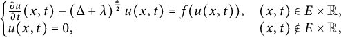 $$ \begin{align} \left\{\begin{array}{@{}ll} \frac{\partial u}{\partial t}(x, t)-\left(\Delta+\lambda\right)^{\frac{\alpha}{2}} u(x, t)=f(u(x, t)), &(x, t) \in E\times \mathbb R,\\ u(x,t)=0, & (x,t) \notin E\times \mathbb R, \end{array} \right. \end{align} $$
where $f(\cdot )$
is non-increasing in the range of u. Assume that there exists
$f(\cdot )$
is non-increasing in the range of u. Assume that there exists $l>0$
such that
$l>0$
such that
 $$ \begin{align} u\geq0 \,\,\,\, \text{in} \,\, \left\{(x,t)=(x',x_n,t)\in E\times \mathbb R\,|\,\varphi(x')<x_{n}<\varphi(x')+l\right\}. \end{align} $$
Then, either $u\equiv 0$
in
$u\equiv 0$
in $\mathbb {R}^{n}\times \mathbb R$
and
$\mathbb {R}^{n}\times \mathbb R$
and $f(0)=0$
, or u is strictly monotone increasing in the
$f(0)=0$
, or u is strictly monotone increasing in the $x_n$
direction; and hence
$x_n$
direction; and hence $u>0$
in
$u>0$
in $E\times \mathbb R$
.
$E\times \mathbb R$
.
Furthermore, suppose E is contained in a half-space, the same conclusion can be reached without the assumption (1.16). Furthermore, if E itself is exactly a half-space, then
 $$ \begin{align*}u(x,t)=u\left(\langle\left(x',x_{n}-\varphi(0')\right),\mathbf{ \nu}\rangle,t\right),\end{align*} $$
where $\mathbf {\nu }$
is the unit inner normal vector to the hyper-plane
$\mathbf {\nu }$
is the unit inner normal vector to the hyper-plane $\partial E$
and
$\partial E$
and $\langle \cdot ,\cdot \rangle $
denotes the inner product in Euclidean space. In particular, if
$\langle \cdot ,\cdot \rangle $
denotes the inner product in Euclidean space. In particular, if $E=\mathbb {R}^{n}_{+}$
, then
$E=\mathbb {R}^{n}_{+}$
, then $u(x,t)=u(x_{n},t)$
.
$u(x,t)=u(x_{n},t)$
.
The article is organized as follows: In Section 2, we establish maximum principles for tempered fractional operators unbounded domains, which is Theorem 1.1. As applications, in Section 3, after extending the sliding methods, we show monotonicity of solutions to the tempered fractional parabolic problem, which are Theorem 1.2. In Section 4, we will prove Theorem 1.4.
From now on and in the following of the article, we always use the same C to denote a constant whose value may be different from line-to-line, and only the relevant dependence is specified.
2 Proof of Theorem 1.1
In this section, we shall establish maximum principles for the parabolic problem involving tempered fractional Laplacian operator $-\left (\Delta +\lambda \right )^{\frac {\alpha }{2}}$
in unbounded domains. These maximum principles are key ingredients in applying the sliding method. We begin with the following a generalized average inequality, which becomes an effective tool in establishing maximum principles in unbounded domains.
$-\left (\Delta +\lambda \right )^{\frac {\alpha }{2}}$
in unbounded domains. These maximum principles are key ingredients in applying the sliding method. We begin with the following a generalized average inequality, which becomes an effective tool in establishing maximum principles in unbounded domains.
Lemma 2.1 (A generalized average inequality)
Assume $u \in {{\mathscr {L}_{\alpha }}(\mathbb {R}^n)} \cap C_{loc}^{1,1}(\mathbb {R}^n)$
. For any
$u \in {{\mathscr {L}_{\alpha }}(\mathbb {R}^n)} \cap C_{loc}^{1,1}(\mathbb {R}^n)$
. For any $r>0$
, if
$r>0$
, if $\bar {x}$
is a maximum point of u in
$\bar {x}$
is a maximum point of u in $B_{r}(\bar {x})$
. Then, we have
$B_{r}(\bar {x})$
. Then, we have
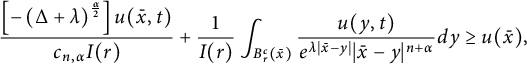 $$ \begin{align} \frac{\left[-\left(\Delta+\lambda\right)^{\frac{\alpha}{2}}\right]u(\bar{x},t)}{c_{n,\alpha}I(r)} +\frac{1}{I(r)}\int_{B_r^c(\bar{x})}\frac{u(y,t)}{e^{\lambda|\bar{x}-y|}|\bar{x}-y|^{{n+\alpha}}}dy \geq u(\bar{x}), \end{align} $$
where the function $I(r)$
is defined by
$I(r)$
is defined by
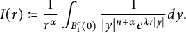
 $$ \begin{align} I(r):=\frac{1}{r^{\alpha}}\int_{B_1^c(0)}\frac{1}{|y|^{{n+\alpha}}e^{\lambda r|y|}}dy. \end{align} $$
Proof By definition of $-\left (\Delta +\lambda \right )^{\frac {\alpha }{2}}$
, we have, for any
$-\left (\Delta +\lambda \right )^{\frac {\alpha }{2}}$
, we have, for any $r>0$
,
$r>0$
,
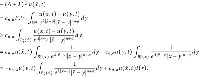 $$ \begin{align*} &-\left(\Delta+\lambda\right)^{\frac{\alpha}{2}}u(\bar{x},t)\\ &=c_{n,\alpha} P.V. \int_{\mathbb{R}^{n}} \frac{u(\bar{x},t)-u(y,t)}{e^{\lambda|\bar{x}-y|}|\bar{x}-y|^{{n+\alpha}}}d y\\ &\geq c_{n,\alpha}\int_{B_r^c(\bar{x})}\frac{u(\bar{x},t)-u(y,t)}{e^{\lambda|\bar{x}-y|}|\bar{x}-y|^{{n+\alpha}}}dy\\ &= c_{n,\alpha}u(\bar{x},t)\int_{B_r^c(\bar{x})}\frac{1}{e^{\lambda|\bar{x}-y|}|\bar{x}-y|^{{n+\alpha}}}dy- c_{n,\alpha}u(y,t)\int_{B_r^c(\bar{x})}\frac{1}{e^{\lambda|\bar{x}-y|}|\bar{x}-y|^{{n+\alpha}}}dy \\ &= - c_{n,\alpha}u(y,t)\int_{B_r^c(\bar{x})}\frac{1}{e^{\lambda|\bar{x}-y|}|\bar{x}-y|^{{n+\alpha}}}dy +c_{n,\alpha}u(\bar{x},t)I(r), \end{align*} $$
provided that
 $$ \begin{align*}I(r):=\frac{1}{r^{\alpha}}\int_{B_1^c(0)}\frac{1}{|y|^{{n+\alpha}}e^{\lambda r|y|}}dy.\\[-46pt] \end{align*} $$
Remark 2.2 In the special case, when u satisfies the following s-subharmonic property at the point $(\bar {x},t)$
:
$(\bar {x},t)$
:
 $$ \begin{align} \left[-\left(\Delta+\lambda\right)^{\frac{\alpha}{2}}\right]u(\bar{x},t)\leq0, \end{align} $$
the average inequality (2.1) becomes
 $$ \begin{align} u(\bar{x})\leq\int_{B_r^c(\bar{x})}u(y)\,d\mu(y) \end{align} $$
with
 $$ \begin{align*}\int_{B_r^c(\bar{x})}d\mu(y)=1.\end{align*} $$
Next, we will prove the maximum principles in unbounded open sets Theorem 1.1.
Proof Suppose that (1.11) is not true, again with $u(x, t)$
is bounded from above in
$u(x, t)$
is bounded from above in $\Omega \times \mathbb {R}$
, then there exists a positive constant A such that
$\Omega \times \mathbb {R}$
, then there exists a positive constant A such that
 $$ \begin{align} \sup _{(x, t) \in \Omega \times \mathbb{R}} u(x, t):=A>0. \end{align} $$
On the other hand, due to the domain $\Omega \times \mathbb {R}$
is unbounded, the supremum of
$\Omega \times \mathbb {R}$
is unbounded, the supremum of $u(x, t)$
may not be attained, then there exists a sequence
$u(x, t)$
may not be attained, then there exists a sequence $\left \{\left (x^k, t_k\right )\right \} \subset \Omega \times \mathbb {R}$
such that
$\left \{\left (x^k, t_k\right )\right \} \subset \Omega \times \mathbb {R}$
such that
 $$ \begin{align*}u\left(x^k, t_k\right) \rightarrow A, \text { as } k \rightarrow \infty. \end{align*} $$
More accurately, there exits a nonnegative sequence $\left \{\varepsilon _k\right \} \searrow 0$
such that
$\left \{\varepsilon _k\right \} \searrow 0$
such that
 $$ \begin{align} u\left(x^k, t_k\right)=A-\varepsilon_k>0. \end{align} $$
From the assumption that $u\leq 0$
in
$u\leq 0$
in $\Omega ^c\times \mathbb R$
and the continuity of u, without loss of generality, we may assume that dist
$\Omega ^c\times \mathbb R$
and the continuity of u, without loss of generality, we may assume that dist $\left \{x^k, \Omega ^c\right \} \geq 1$
. Now, we define the following auxiliary function:
$\left \{x^k, \Omega ^c\right \} \geq 1$
. Now, we define the following auxiliary function:
 $$ \begin{align*}v_k(x, t)=u(x, t)+\varepsilon_k \psi_k(x, t), \end{align*} $$
where $\psi _k(x, t)=\psi \left (\frac {x-x^k}{r \cdot e^{\lambda r}}, \frac {t-t_k}{ r^{\alpha } \cdot e^{3\lambda r}}\right )$
with any fixed
$\psi _k(x, t)=\psi \left (\frac {x-x^k}{r \cdot e^{\lambda r}}, \frac {t-t_k}{ r^{\alpha } \cdot e^{3\lambda r}}\right )$
with any fixed $r>0$
and
$r>0$
and $\psi (x, t)$
is given by
$\psi (x, t)$
is given by
 $$ \begin{align*}\psi (x, t)= \begin{cases}1, & \text { if }|(x, t)| \leq \frac{1}{2}, \\ 0, & \text { if }|(x, t)| \geq 1. \end{cases} \end{align*} $$
It is well known that $\psi \in C_0^{\infty }\left (\mathbb {R}^n \times \mathbb {R}\right )$
, therefore
$\psi \in C_0^{\infty }\left (\mathbb {R}^n \times \mathbb {R}\right )$
, therefore $|\left (\Delta +\lambda \right )^{\frac {\alpha }{2}}\psi (x,t)|\leq C_0$
for any
$|\left (\Delta +\lambda \right )^{\frac {\alpha }{2}}\psi (x,t)|\leq C_0$
for any $x \in \mathbb {R}^n\times \mathbb {R}$
.
$x \in \mathbb {R}^n\times \mathbb {R}$
.
Next, for convenience, we denote
 $$ \begin{align*}Q_{r e^{\lambda r}}\left(x^k, t_k\right):=\left\{(x, t)|\left(\frac{x-x^k}{r \cdot e^{\lambda r}}, \frac{t-t_k}{r^{\alpha}e^{3\lambda r}}\right) \mid<1\right\}. \end{align*} $$
It is easy to see that
 $$ \begin{align*}\max_{x\in Q_{r e^{\lambda r}}\left(x^k, t_k\right)}v_k(x, t)\geq \max_{x\in Q_{r e^{\lambda r}}^{c}\left(x^k, t_k\right)}v_k(x, t), \end{align*} $$
which implies the maximum value of $v_k(x, t)$
in
$v_k(x, t)$
in $\mathbb {R}^n \times \mathbb {R}$
is attained in
$\mathbb {R}^n \times \mathbb {R}$
is attained in $Q_{r e^{\lambda r}}\left (x^k, t_k\right )$
along which we will be able to derive a contradiction. More precisely, one can infer from the definition of
$Q_{r e^{\lambda r}}\left (x^k, t_k\right )$
along which we will be able to derive a contradiction. More precisely, one can infer from the definition of $v_k(x, t)$
and (2.6), we know that
$v_k(x, t)$
and (2.6), we know that
 $$ \begin{align*}v_k\left(x^k, t_k\right)=A>0. \end{align*} $$
On the other hand, for any $(x, t) \in \left (\mathbb {R}^n \times \mathbb {R}\right ) \backslash Q_{r e^{\lambda r}}\left (x^k, t_k\right )$
, we have
$(x, t) \in \left (\mathbb {R}^n \times \mathbb {R}\right ) \backslash Q_{r e^{\lambda r}}\left (x^k, t_k\right )$
, we have
 $$ \begin{align*}v_k(x, t) \leq A. \end{align*} $$
Consequently, there exists $\left (\bar {x}^k, \bar {t}_k\right )\in Q_{r e^{\lambda r}} \left (x^k, t_k\right )$
such that
$\left (\bar {x}^k, \bar {t}_k\right )\in Q_{r e^{\lambda r}} \left (x^k, t_k\right )$
such that
 $$ \begin{align} A+\varepsilon_k \geq v_k\left(\bar{x}^k, \bar{t}_k\right)=\sup _{(x, t) \in \mathbb{R}^n \times \mathbb{R}} v_k(x, t) \geq A>0. \end{align} $$
Through direct computation, it follows that
 $$ \begin{align*}-\left(\Delta+\lambda\right)^{\frac{\alpha}{2}} v_k\left(\bar{x}^k, \bar{t}_k\right)=c_{n, \alpha} P.V. \int_{\mathbb{R}^n} \frac{v_k\left(\bar{x}^k, \bar{t}_k\right)-v_k\left(y, \bar{t}_k\right)}{e^{\lambda\left|\bar{x}^k-y\right|}\left|\bar{x}^k-y\right|{}^{n+\alpha}} d y \geq 0, \end{align*} $$
and
 $$ \begin{align*}\frac{\partial v_k}{\partial t}\left(\bar{x}^k, \bar{t}_k\right)=0. \end{align*} $$
And hence,
 $$ \begin{align*}\left|\frac{\partial u}{\partial t}\left(\bar{x}^k, \bar{t}_k\right)\right|=\left|\frac{\partial v_k}{\partial t}\left(\bar{x}^k, \bar{t}_k\right)-\varepsilon_k \frac{\partial \psi_k}{\partial t}\left(\bar{x}^k, \bar{t}_k\right)\right| \leq \frac{C \varepsilon_k}{{r^{\alpha}e^{3 \lambda r}}}. \end{align*} $$
Collecting the above estimates, we obtain
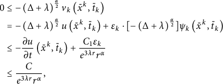 $$ \begin{align} \begin{aligned} 0& \leq-\left(\Delta+\lambda\right)^{\frac{\alpha}{2}} v_k\left(\bar{x}^k, \bar{t}_k\right) \\ & =-\left(\Delta+\lambda\right)^{\frac{\alpha}{2}}u\left(\bar{x}^k, \bar{t}_k\right)+\varepsilon_k\cdot[-\left(\Delta+\lambda\right)^{\frac{\alpha}{2}}] \psi_k\left(\bar{x}^k, \bar{t}_k\right) \\ & \leq-\frac{\partial u}{\partial t}\left(\bar{x}^k, \bar{t}_k\right)+\frac{C_1 \varepsilon_k}{e^{3\lambda r} r^{\alpha}} \\ & \leq \frac{C}{e^{3\lambda r} r^{\alpha}}, \end{aligned} \end{align} $$
where we have use the truth of
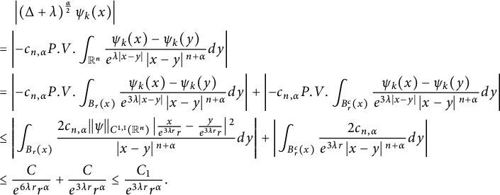 $$ \begin{align} &\quad \,\left|\left(\Delta+\lambda\right)^{\frac{\alpha}{2}} \psi_{k}(x)\right|\\&=\left|-c_{n,\alpha}P.V.\int_{\mathbb{R}^{n}}\frac{\psi_{k}(x) -\psi_{k}(y)}{e^{\lambda|{x}-y|}\left|{x}-y\right|{}^{{n+\alpha}}}dy\right| \nonumber \\ &=\left|-c_{n,\alpha}P.V.\int_{B_{r}(x)}\frac{\psi_{k}(x) -\psi_{k}(y)}{e^{3\lambda|{x}-y|}\left|{x}-y\right|{}^{{n+\alpha}}}dy\right|+\left|-c_{n,\alpha}P.V.\int_{B_{r }^{c}(x)}\frac{\psi_{k}(x) -\psi_{k}(y)}{e^{3\lambda|{x}-y|}\left|{x}- y\right|{}^{{n+\alpha}}}dy\right| \nonumber \\ &\leq \left|\int_{B_{r}(x)}\frac{2c_{n,\alpha}||\psi||_{C^{1,1}(\mathbb R^n)}\left|\frac{x}{e^{3\lambda r}r}-\frac{y}{e^{3\lambda r}r}\right|{}^{2}}{\left|{x}-y\right|{}^{{n+\alpha}}}dy\right|+\left|\int_{B_{r }^{c}(x)}\frac{2 c_{n,\alpha}}{e^{3 \lambda r}\left|{x}-y\right|{}^{{n+\alpha}}}dy\right| \nonumber\\ &\leq \frac{C}{e^{6\lambda r}r^{\alpha}}+\frac{C}{e^{3\lambda r} r^{\alpha}}\leq \frac{C_1}{e^{3\lambda r} r^{\alpha}}.\nonumber \end{align} $$
Recalling Theorem 2.1, we know that, for any $r>0$
,
$r>0$
,
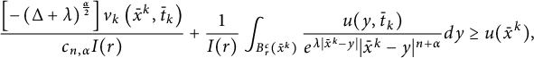 $$ \begin{align} \frac{\left[-\left(\Delta+\lambda\right)^{\frac{\alpha}{2}}\right]v_k\left(\bar{x}^k, \bar{t}_k\right)}{c_{n,\alpha}I(r)}+\frac{1}{I(r)}\int_{B_r^c(\bar{x}^k)}\frac{u(y,\bar{t}_k)}{e^{\lambda|\bar{x}^k-y|}|\bar{x}^k-y|^{{n+\alpha}}}dy \geq u(\bar{x}^k), \end{align} $$
where
 $$ \begin{align*}I(r):=\frac{1}{r^{\alpha}}\int_{B_1^c(0)}\frac{1}{|y|^{{n+\alpha}}e^{\lambda r|y|}}dy. \end{align*} $$
Next, we shall prove that the left-hand side of the inequality (2.10) is strictly less than A. Indeed, after a simple calculation, we get
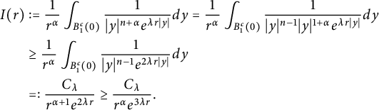 $$ \begin{align} \begin{aligned} I(r)& :=\frac{1}{r^{\alpha}}\int_{B_1^c(0)}\frac{1}{|y|^{{n+\alpha}}e^{\lambda r|y|}}dy=\frac{1}{r^{\alpha}}\int_{B_1^c(0)}\frac{1}{|y|^{n-1}|y|^{1+\alpha}e^{\lambda r|y|}}dy \\ & \geq \frac{1}{r^{\alpha}}\int_{B_1^c(0)}\frac{1}{|y|^{n-1}e^{2\lambda r|y|}}dy \\ & =:\frac{C_\lambda}{r^{\alpha+1}e^{2\lambda r}}\geq\frac{C_\lambda}{r^{\alpha}e^{3\lambda r}}. \end{aligned} \end{align} $$
Again with (2.8), we derive that
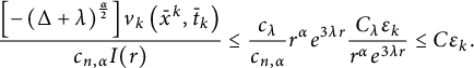 $$ \begin{align*}\frac{\left[-\left(\Delta+\lambda\right)^{\frac{\alpha}{2}}\right]v_k\left(\bar{x}^k, \bar{t}_k\right)}{c_{n,\alpha}I(r)} \leq \frac{c_\lambda}{c_{n, \alpha}} {r^{\alpha} e^{3\lambda r}} \frac{C_\lambda \varepsilon_k}{r^{\alpha}e^{3\lambda r}} \leq C \varepsilon_k. \end{align*} $$
Therefore, our goals is to estimate the upper bound of the second term in (2.10). First, since $R>R / \sqrt [n]{2}$
, combine this with assumption (1.9), we know that
$R>R / \sqrt [n]{2}$
, combine this with assumption (1.9), we know that
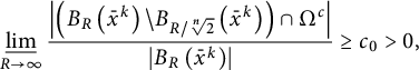 $$ \begin{align} \varliminf_{R \rightarrow \infty} \frac{\left|\left(B_R\left(\bar{x}^k\right) \backslash B_{R / \sqrt[n]{2}}\left(\bar{x}^k\right)\right) \cap \Omega^c\right|}{\left|B_R\left(\bar{x}^k\right)\right|}\geq c_0>0, \end{align} $$
which indicates that there exist two positive constants $\bar {C}$
and sufficiently large
$\bar {C}$
and sufficiently large $R_k$
such that
$R_k$
such that
 $$ \begin{align} \frac{\left|\left(B_R\left(\bar{x}^k\right) \backslash B_{R / \sqrt[n]{2}}\left(\bar{x}^k\right)\right) \cap \Omega^c\right|}{\left|B_R\left(\bar{x}^k\right)\right|} \geq \bar{C}>0, \quad R \geq R_k. \end{align} $$
Combining (2.5) and (2.13), taking $r=R_k / \sqrt [n]{2}$
and noting the fact
$r=R_k / \sqrt [n]{2}$
and noting the fact
 $$ \begin{align*}v_k\left(y, \bar{t}_k\right)=u\left(y, \bar{t}_k\right) \leq 0, y \in B_r^c\left(\bar{x}^k\right) \cap \Omega^c, \end{align*} $$
we obtain
 $$ \begin{align} \begin{aligned} &\qquad \frac{1}{I(r)}\int_{B_r^c(\bar{x}^k)}\frac{u(y,\bar{t}_k)}{e^{\lambda|\bar{x}^k-y|}|\bar{x}^k-y|^{{n+\alpha}}}dy\\ & =\frac{1}{I\left((\frac{R_k}{\sqrt[n]{2}} )^{\alpha}\right)} \int_{B_{R_k /{\sqrt[n]{2}}}^c\left(\bar{x}^k\right)} \frac{v_k\left(y, \bar{t}_k\right)}{e^{\lambda|\bar{x}^k-y|}\left|\bar{x}^k-y\right|{}^{n+\alpha}} d y\\ & =\frac{1}{I\left((R_k / \sqrt[n]{2})^{\alpha}\right)} \left(\int_{B_{R_k /{\sqrt[n]{2}}}^c\left(\bar{x}^k\right) \cap \Omega} \frac{v_k\left(y, \bar{t}_k\right)}{e^{\lambda|\bar{x}^k-y|}\left|\bar{x}^k-y\right|{}^{{n+\alpha}}} d y+\int_{B_{R_k / k_2\left(\bar{x}^k\right) \cap \Omega^c}} \frac{A+\varepsilon_k}{e^{\lambda|\bar{x}^k-y|}\left|\bar{x}^k-y\right|{}^{{n+\alpha}}} d y \right.\\ &\quad \left.-\int_{B_{R_k / \sqrt[n]{2}}^c\left(\bar{x}^k\right) \cap \Omega^c} \frac{A+\varepsilon_k}{e^{\lambda|\bar{x}^k-y|}\left|\bar{x}^k-y\right|{}^{{n+\alpha}}} d y+\int_{B_{R_k / \sqrt[n]{2}}^c\left(\bar{x}^k\right) \cap \Omega^c} \frac{v_k\left(y, \bar{t}_k\right)}{e^{\lambda|\bar{x}^k-y|}\left|\bar{x}^k-y\right|{}^{{n+\alpha}}} d y\right)\\ &\leq \frac{1}{I\left((R_k / \sqrt[n]{2})^{\alpha}\right)} \int_{B_{R_k /{\sqrt[n]{2}}}^c(\bar{x}^k) } \frac{A+\varepsilon_k}{e^{\lambda|\bar{x}^k-y|}\left|\bar{x}^k-y\right|{}^{{n+\alpha}}} d y\\ &\quad-\frac{1}{I\left((R_k / \sqrt[n]{2})^{\alpha}\right)} \int_{B_{R_k /{\sqrt[n]{2}}}^c(\bar{x}^k) \cap \Omega^c} \frac{A+\varepsilon_k}{e^{\lambda|\bar{x}^k-y|}\left|\bar{x}^k-y\right|{}^{{n+\alpha}}} d y\\ &= A+\varepsilon_k-\frac{1}{I\left((R_k / \sqrt[n]{2})^{\alpha}\right)} \int_{B_{R_k /{\sqrt[n]{2}}}^c(\bar{x}^k) \cap \Omega^c} \frac{A+\varepsilon_k}{e^{\lambda|\bar{x}^k-y|}\left|\bar{x}^k-y\right|{}^{{n+\alpha}}} d y\\ &\leq A+\varepsilon_k-\frac{1}{I\left((R_k / \sqrt[n]{2})^{\alpha}\right)} \int_{[B_{R_k}(\bar{x}^k)\setminus B_{R_k /{\sqrt[n]{2}}}^c(\bar{x}^k)] \cap \Omega^c} \frac{A+\varepsilon_k}{e^{\lambda|\bar{x}^k-y|}\left|\bar{x}^k-y\right|{}^{{n+\alpha}}} d y\\ &\leq A+\varepsilon_k-\frac{A+\varepsilon_k}{I\left((R_k / \sqrt[n]{2})^{\alpha}\right)}{\left|[B_{R_k}(\bar{x}^k)\setminus B_{R_k /{\sqrt[n]{2}}}^c(\bar{x}^k)]\cap \Omega^c \right| } \frac{1}{e^{\lambda\frac{R_k}{\sqrt[n]{2}} }\left|\frac{R_k}{\sqrt[n]{2}} \right|{}^{{n+\alpha}}}\\ &\leq A+\varepsilon_k-\frac{A+\varepsilon_k}{{C_\lambda}}{\left(\frac{R_k}{\sqrt[n]{2}}\right)^{\alpha+1}e^{2\lambda \cdot {\frac{R_k}{\sqrt[n]{2}}}}}{\left|[B_{R_k}(\bar{x}^k)\setminus B_{R_k /{\sqrt[n]{2}}}^c(\bar{x}^k)]\cap \Omega^c \right| } \frac{1}{e^{\lambda\frac{R_k}{\sqrt[n]{2}} }\left|\frac{R_k}{\sqrt[n]{2}} \right|{}^{{n+\alpha}}}\\ &\leq \left(A+\varepsilon_k\right)(1-C_\lambda). \end{aligned} \end{align} $$
Combining (2.8)–(2.14), we know that
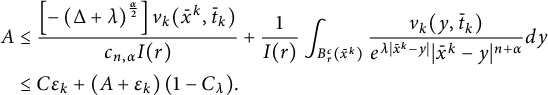 $$ \begin{align} \begin{aligned} A& \leq\frac{\left[-\left(\Delta+\lambda\right)^{\frac{\alpha}{2}}\right]v_k(\bar{x}^k,\bar{t}_k)}{c_{n,\alpha}I(r)} +\frac{1}{I(r)}\int_{B_r^c(\bar{x}^{k})}\frac{v_k(y,\bar{t}_k)}{e^{\lambda|\bar{x}^k-y|}|\bar{x}^{k}-y|^{{n+\alpha}}}dy \\ & \leq C \varepsilon_k+\left(A+\varepsilon_k\right)(1-C_\lambda). \end{aligned} \end{align} $$
We can immediately get the contradiction as $k\rightarrow \infty $
. Therefore, conclusion (1.11) must holds.
$k\rightarrow \infty $
. Therefore, conclusion (1.11) must holds.
3 Proof of Theorem 1.4
In this section, based on Theorem 1.1, combining with direct sliding method, we shall prove Theorem 1.4.
First of all, we give some useful notations, for any $x=(x', {x_n})$
with
$x=(x', {x_n})$
with $x':= ({x_1},...,{x_{n-1}}) \in {\mathbb {R}^{n-1}}$
and
$x':= ({x_1},...,{x_{n-1}}) \in {\mathbb {R}^{n-1}}$
and $\tau \in \mathbb {R}$
, we denote:
$\tau \in \mathbb {R}$
, we denote:
- $\bullet\ x^{\tau }=x+\tau e_n, \quad \text {with}\,\,\,\,e_n=(0^{'},1)$
,
$\bullet\ x^{\tau }=x+\tau e_n, \quad \text {with}\,\,\,\,e_n=(0^{'},1)$
, -
$\bullet\ u_\tau (x,t):=u(x', x_n+\tau ,t),$
-
$\bullet\ w_\tau (x,t):=u(x,t)-u_\tau (x,t).$


Proof
Step 1. We prove that for $\tau $
sufficiently large, we have
$\tau $
sufficiently large, we have
 $$ \begin{align} w_\tau(x, t) \leq 0,\qquad (x, t) \in \mathbb{R}^n \times \mathbb{R}. \end{align} $$
Recalling assumption (1.13), then there exists a sufficiently large $a>0$
such that
$a>0$
such that
 $$ \begin{align} |u(x, t)| \geq 1-\delta \text { for }\left|x_n\right| \geq a,\left(x^{\prime}, t\right) \in \mathbb{R}^{n-1} \times \mathbb{R}. \end{align} $$
Suppose (3.1) is violated, then there exists a constant $A>0$
such that
$A>0$
such that
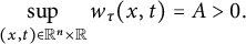 $$ \begin{align*}\sup _{(x, t) \in \mathbb{R}^n \times \mathbb{R}} w_\tau(x, t)=A>0. \end{align*} $$
In order to derive a contradiction with $(3.5)$
, we consider the function
$(3.5)$
, we consider the function
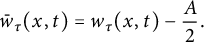 $$ \begin{align*}\bar{w}_\tau(x, t)=w_\tau(x, t)-\frac{A}{2}. \end{align*} $$
Our aim is to show that
 $$ \begin{align*}\bar{w}_\tau(x, t) \leq 0,(x, t) \in \mathbb{R}^n \times \mathbb{R}. \end{align*} $$
One can infer from assumption (1.13) that, for all $t \in \mathbb {R}$
, we can choose a sufficiently large constant
$t \in \mathbb {R}$
, we can choose a sufficiently large constant $M>a$
such that
$M>a$
such that
 $$ \begin{align} \bar{w}_\tau(x, t) \leq 0,\quad \text{for} \,\,\,x_n \geq M,\left(x^{\prime}, t\right) \in \mathbb{R}^{n-1} \times \mathbb{R}. \end{align} $$
Denote
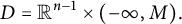 $$ \begin{align*}D=\mathbb{R}^{n-1} \times(-\infty, M). \end{align*} $$
Then equation (3.3) implies
 $$ \begin{align} \bar{w}_\tau(x, t) \leq 0,(x, t) \in D^c \times \mathbb{R}. \end{align} $$
That implies $\bar {w}_\tau (x, t)$
satisfies the exterior condition in Theorem 1.1.
$\bar {w}_\tau (x, t)$
satisfies the exterior condition in Theorem 1.1.
Consequently, equation (2.13) implies that $\bar {w}_\tau (x, t)$
satisfies
$\bar {w}_\tau (x, t)$
satisfies
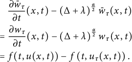 $$ \begin{align} \begin{aligned} & \quad \frac{\partial \bar{w}_\tau}{\partial t}(x, t)-\left(\Delta+\lambda\right)^{\frac{\alpha}{2}} \bar{w}_\tau(x, t) \\ & = \frac{\partial w_\tau}{\partial t}(x, t)-\left(\Delta+\lambda\right)^{\frac{\alpha}{2}} w_\tau(x, t) \\ & = f(t, u(x, t))-f\left(t, u_\tau(x, t)\right). \end{aligned} \end{align} $$
Next, we claim that, for any $\left (x^{\prime }, t\right ) \in \mathbb {R}^{n-1} \times \mathbb {R}$
, we have
$\left (x^{\prime }, t\right ) \in \mathbb {R}^{n-1} \times \mathbb {R}$
, we have
 $$ \begin{align} f(t, u(x, t)) \leq f\left(t, u_\tau(x, t)\right), \,\,\text{at the points where}\,\, w_\tau(x, t)>0. \end{align} $$
We will prove our claim (3.6) by discussing three different cases.
Case (i): $\left |x_n\right | \leq a$
. For any
$\left |x_n\right | \leq a$
. For any $\tau \geq 2 a$
, then
$\tau \geq 2 a$
, then $x_n+\tau \geq a$
, again with (3.2), at the points where
$x_n+\tau \geq a$
, again with (3.2), at the points where $w_\tau (x, t)>0$
, we have
$w_\tau (x, t)>0$
, we have
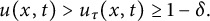 $$ \begin{align*}u(x, t)>u_\tau(x, t) \geq 1-\delta. \end{align*} $$
Combine this truth with the monotonicity assumption (1.14) on the function f, one can immediately get claim (3.6).
Case (ii): $x_n<-a$
. For any
$x_n<-a$
. For any $\left (x^{\prime }, t\right ) \in \mathbb {R}^{n-1} \times \mathbb {R}$
, by assumption (1.13) and (3.2), we get
$\left (x^{\prime }, t\right ) \in \mathbb {R}^{n-1} \times \mathbb {R}$
, by assumption (1.13) and (3.2), we get
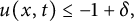 $$ \begin{align*}u(x, t) \leq-1+\delta, \end{align*} $$
and therefore at the points where $w_\tau (x, t)>0$
,
$w_\tau (x, t)>0$
,
 $$ \begin{align*}u_\tau(x, t)<u(x, t) \leq-1+\delta, \end{align*} $$
which implies that we can use the monotonicity assumption (1.14) on the function f to derive claim (3.6).
Case (iii): $x_n>a$
. For any
$x_n>a$
. For any $\left (x^{\prime }, t\right ) \in \mathbb {R}^{n-1} \times \mathbb {R}$
, by (3.2), we have, at the points where
$\left (x^{\prime }, t\right ) \in \mathbb {R}^{n-1} \times \mathbb {R}$
, by (3.2), we have, at the points where $w_\tau (x, t)>0$
,
$w_\tau (x, t)>0$
,
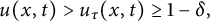 $$ \begin{align*}u(x, t)>u_\tau(x, t) \geq 1-\delta, \end{align*} $$
and therefore, we use the monotonicity assumption (1.14) on the function f again to derive claim (3.6). Thus, our claim (3.6) must hold.
One can infer from (3.6) that
 $$ \begin{align*}\frac{\partial \bar{w}_\tau}{\partial t}(x, t)-\left(\Delta+\lambda\right)^{\frac{\alpha}{2}} \bar{w}_\tau(x, t) \leq 0, \text { at the points in } D \times \mathbb{R,} \text { where } w_\tau(x, t)>0 \text {. } \end{align*} $$
This is also valid at the points in $D \times \mathbb {R,}$
where
$D \times \mathbb {R,}$
where $\bar {w}_\tau (x, t)>0$
, more precisely,
$\bar {w}_\tau (x, t)>0$
, more precisely,
 $$ \begin{align*}\frac{\partial \bar{w}_\tau}{\partial t}(x, t)-\left(\Delta+\lambda\right)^{\frac{\alpha}{2}} \bar{w}_\tau(x, t) \leq 0 \text {, at the points in } D \times \mathbb{R,} \text { where } \bar{w}_\tau(x, t)>0, \end{align*} $$
which together with the exterior condition on $\bar {w}_\tau (x, t)$
(3.4), and the maximum principle in unbounded domains (Theorem 1.1) implies
$\bar {w}_\tau (x, t)$
(3.4), and the maximum principle in unbounded domains (Theorem 1.1) implies
 $$ \begin{align*}\bar{w}_\tau(x, t) \leq 0,(x, t) \in \mathbb{R}^n \times \mathbb{R}. \end{align*} $$
It follows that
 $$ \begin{align*}w_\tau(x, t) \leq \frac{A}{2},(x, t) \in \mathbb{R}^n \times \mathbb{R,} \end{align*} $$
which contradicts the truth of $\sup _{(x, t) \in \mathbb {R}^n \times \mathbb {R}} w_\tau (x, t)=A>0$
. Therefore,
$\sup _{(x, t) \in \mathbb {R}^n \times \mathbb {R}} w_\tau (x, t)=A>0$
. Therefore, $w_\tau (x, t) \leq 0$
, for any
$w_\tau (x, t) \leq 0$
, for any $\tau \geq 2 a$
and
$\tau \geq 2 a$
and $(x, t) \in \mathbb {R}^n \times \mathbb {R}$
. This completes the proof in Step 1.
$(x, t) \in \mathbb {R}^n \times \mathbb {R}$
. This completes the proof in Step 1.
Step 2. Inequality (3.1) provides a starting point for us to carry out the sliding procedure. In this step, we decrease $\tau $
from close to
$\tau $
from close to $\tau =2 a$
to
$\tau =2 a$
to $0$
, and prove that for any
$0$
, and prove that for any $0<\tau <2 a$
, we still have
$0<\tau <2 a$
, we still have
 $$ \begin{align} w_\tau(x, t) \leq 0,(x, t) \in \mathbb{R}^n \times \mathbb{R}. \end{align} $$
To this end, we define
 $$ \begin{align*}\tau_0=\inf \left\{\tau \mid w_\tau(x, t) \leq 0,(x, t) \in \mathbb{R}^n \times \mathbb{R}\right\}, \end{align*} $$
and prove that $\tau _0=0$
. Otherwise, we show that
$\tau _0=0$
. Otherwise, we show that $\tau _0$
can be decreased a little bit while inequality
$\tau _0$
can be decreased a little bit while inequality
 $$ \begin{align*}w_\tau(x, t) \leq 0,(x, t) \in \mathbb{R}^n \times \mathbb{R}, \tau \in\left(\tau_0-\varepsilon, \tau_0\right] \end{align*} $$
is still valid, which contradicts the definition of $\tau _0$
.
$\tau _0$
.
(I) We first show that
 $$ \begin{align} \sup _{\left|x_n\right| \leq a,\left(x^{\prime}, t\right) \in \mathbb{R}^{n-1} \times \mathbb{R}} w_{\tau_0}(x, t)<0. \end{align} $$
Suppose (3.14) is false, then
 $$ \begin{align*}\sup _{\left|x_n\right| \leq a_1\left(x^{\prime}, t\right) \in \mathbb{R}^{n-1} \times \mathbb{R}} w_{\tau_0}(x, t)=0, \end{align*} $$
and there exists a sequence
 $$ \begin{align*}\left\{\left(x^k, t_k\right)\right\} \subset\left(\mathbb{R}^{n-1} \times[-a, a]\right) \times \mathbb{R},\,\, k=1,2, \ldots, \end{align*} $$
such that
 $$ \begin{align*}w_{\tau_0}\left(x^k, t_k\right) \rightarrow 0,\,\, \text { as } k \rightarrow \infty. \end{align*} $$
More precisely, there exist a nonnegative sequence $\left \{\varepsilon _k\right \} \searrow 0$
such that
$\left \{\varepsilon _k\right \} \searrow 0$
such that
 $$ \begin{align} w_{\tau_0}\left(x^k, t_k\right)=-\varepsilon_k. \end{align} $$
In order to obtain more information from the supremum of $w_{\tau _0}(x, t)$
, we introduce the following auxiliary function:
$w_{\tau _0}(x, t)$
, we introduce the following auxiliary function:
 $$ \begin{align*}w_k(x, t)=w_{\tau_0}(x, t)+\varepsilon_k \eta_k(x, t) , \end{align*} $$
where
 $$ \begin{align*}\eta_k(x, t)=\eta\left(x-x^k, t-t_k\right) \end{align*} $$
with $\eta (x, t) \in C_0^{\infty }\left (\mathbb {R}^n \times \mathbb {R}\right )$
and
$\eta (x, t) \in C_0^{\infty }\left (\mathbb {R}^n \times \mathbb {R}\right )$
and
 $$ \begin{align*}\eta(x, t)= \begin{cases}1, & \text { if }|(x, t)| \leq \frac{1}{2}, \\ 0, & \text { if }|(x, t)| \geq 1.\end{cases} \end{align*} $$
Denote
 $$ \begin{align*}Q_1\left(x^k, t_k\right):=\left\{(x, t)||(x, t)-\left(x^k, t_k\right) \mid<1\right\}. \end{align*} $$
We can observe that
 $$ \begin{align*}\max_{x\in Q_{1}\left(x^k, t_k\right)}v_k(x, t)\geq \max_{x\in Q_{1}^{c}\left(x^k, t_k\right)}v_k(x, t). \end{align*} $$
Therefore, the maximum value of $w_k(x, t)$
in
$w_k(x, t)$
in $\mathbb {R}^n \times \mathbb {R}$
is attained in
$\mathbb {R}^n \times \mathbb {R}$
is attained in $Q_1\left (x^k, t_k\right )$
, along which we will be able to derive a contradiction. More precisely, from the definition of
$Q_1\left (x^k, t_k\right )$
, along which we will be able to derive a contradiction. More precisely, from the definition of $w_k(x, t)$
and (3.9), one has
$w_k(x, t)$
and (3.9), one has
 $$ \begin{align*}w_k\left(x^k, t_k\right)=0. \end{align*} $$
On the other hand, for $(x, t) \in \left (\mathbb {R}^n \times \mathbb {R}\right ) \backslash Q_1\left (x^k, t_k\right )$
, since
$(x, t) \in \left (\mathbb {R}^n \times \mathbb {R}\right ) \backslash Q_1\left (x^k, t_k\right )$
, since $\eta _k(x, t)=0$
, we get
$\eta _k(x, t)=0$
, we get
 $$ \begin{align*}w_k(x, t) \leq 0. \end{align*} $$
Therefore, $w_k(x, t)$
attains its maximum value in
$w_k(x, t)$
attains its maximum value in $Q_1\left (x^k, t_k\right )$
, say at
$Q_1\left (x^k, t_k\right )$
, say at $\left (\bar {x}^k, \bar {t}_k\right )$
, i.e.,
$\left (\bar {x}^k, \bar {t}_k\right )$
, i.e.,
 $$ \begin{align*}\varepsilon_k \geq w_k\left(\bar{x}^k, \bar{t}_k\right)=\sup _{(x, t) \in \mathbb{R}^n \times \mathbb{R}} w_k(x, t) \geq 0. \end{align*} $$
To simplify the notion, we introduce the following auxiliary function:
 $$ \begin{align} \bar{w}_k(x, t)=w_k\left(x+\bar{x}^k, t+\bar{t}_k\right), \end{align} $$
which implies
 $$ \begin{align} \varepsilon_k \geq \bar{w}_k(0,0)=\sup _{(x, t) \in \mathbb{R}^n \times \mathbb{R}} \bar{w}_k(x, t) \geq 0, \end{align} $$
it follows that
 $$ \begin{align*}-\left(\Delta+\lambda\right)^{\frac{\alpha}{2}} \bar{w}_k(0,0)=C_{n, s} P. V. \int_{\mathbb{R}^n} \frac{\bar{w}_k(0,0)-\bar{w}_k(y, 0)}{e^{\lambda |y|}|y|^{n+\alpha}} d y \geq 0 \end{align*} $$
and
 $$ \begin{align*}\frac{\partial \bar{w}_k}{\partial t}(0,0)=0. \end{align*} $$
Through direct calculations, combine with the truth of $w_{\tau _0}\left (\bar {x}^k, \bar {t}_k\right ) \rightarrow 0 \text {, as } k \rightarrow \infty $
, we derive that
$w_{\tau _0}\left (\bar {x}^k, \bar {t}_k\right ) \rightarrow 0 \text {, as } k \rightarrow \infty $
, we derive that
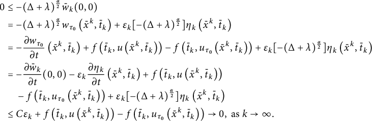 $$ \begin{align} \begin{aligned} 0 & \leq-(\Delta+\lambda)^{\frac{\alpha}{2}} \bar{w}_k(0,0) \\ &=-(\Delta+\lambda)^{\frac{\alpha}{2}} w_{\tau_0}\left(\bar{x}^k, \bar{t}_k\right)+\varepsilon_k[-(\Delta+\lambda)^{\frac{\alpha}{2}} ] \eta_k\left(\bar{x}^k, \bar{t}_k\right) \\ &=-\frac{\partial w_{\tau_0}}{\partial t}\left(\bar{x}^k, \bar{t}_k\right)+f\left(\bar{t}_k, u\left(\bar{x}^k, \bar{t}_k\right)\right)-f\left(\bar{t}_k, u_{\tau_0}\left(\bar{x}^k, \bar{t}_k\right)\right)+\varepsilon_k[-(\Delta+\lambda)^{\frac{\alpha}{2}} ] \eta_k\left(\bar{x}^k, \bar{t}_k\right) \\ &=-\frac{\partial \bar{w}_k}{\partial t}(0,0)-\varepsilon_k \frac{\partial \eta_k}{\partial t}\left(\bar{x}^k, \bar{t}_k\right)+f\left(\bar{t}_k, u\left(\bar{x}^k, \bar{t}_k\right)\right)\\ &\quad -f\left(\bar{t}_k, u_{\tau_0}\left(\bar{x}^k, \bar{t}_k\right)\right)+\varepsilon_k[-(\Delta+\lambda)^{\frac{\alpha}{2}} ] \eta_k\left(\bar{x}^k, \bar{t}_k\right) \\ & \leq C \varepsilon_k+f\left(\bar{t}_k, u\left(\bar{x}^k, \bar{t}_k\right)\right)-f\left(\bar{t}_k, u_{\tau_0}\left(\bar{x}^k, \bar{t}_k\right)\right) \rightarrow 0, \text { as } k \rightarrow \infty. \end{aligned} \end{align} $$
Putting (3.10) and Theorem 1.1 together, we deduce
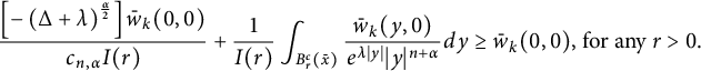 $$ \begin{align} \frac{\left[-\left(\Delta+\lambda\right)^{\frac{\alpha}{2}}\right]\bar{w}_k(0,0)}{c_{n,\alpha}I(r)} +\frac{1}{I(r)}\int_{B_r^c(\bar{x})}\frac{\bar{w}_k(y,0)}{e^{\lambda|y|}|y|^{{n+\alpha}}}dy \geq \bar{w}_k(0,0) \text {, for any } r>0. \end{align} $$
Therefore, we can deduce by using (3.12) and the above average inequality (3.13) that for any finite $r>0$
,
$r>0$
,
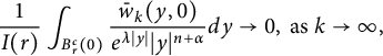 $$ \begin{align*}\frac{1}{I(r)}\int_{B_r^{c}(0)} \frac{\bar{w}_k(y, 0)}{e^{\lambda|y|}|y|^{n+{\alpha}}} d y \rightarrow 0, \text { as } k \rightarrow \infty, \end{align*} $$
which implies that for any fixed $r>0$
,
$r>0$
,
 $$ \begin{align} \bar{w}_k(y, 0) \rightarrow 0, y \in B_r^c(0) \text {, as } k \rightarrow \infty. \end{align} $$
Due to $u(x, t)$
is uniformly continuous, by Arzelà–Ascoli theorem, up to extraction of a subsequence of
$u(x, t)$
is uniformly continuous, by Arzelà–Ascoli theorem, up to extraction of a subsequence of $u_k(x, t):=u\left (x+\bar {x}^k, t+\bar {t}_k\right )$
(still denoted by itself), we obtain
$u_k(x, t):=u\left (x+\bar {x}^k, t+\bar {t}_k\right )$
(still denoted by itself), we obtain
 $$ \begin{align*}u_k(x, t) \rightarrow u_{\infty}(x, t),(x, t) \in \mathbb{R}^n \times \mathbb{R} \text {, as } k \rightarrow \infty, \end{align*} $$
which together with (3.14), yields
 $$ \begin{align*}u_{\infty}(x, 0)-\left(u_{\infty}\right)_{\tau_0}(x, 0) \equiv 0, x \in B_r^c(0). \end{align*} $$
Therefore, for any $j \in \mathbb {N}$
and any fixed
$j \in \mathbb {N}$
and any fixed $r>0$
, we obtain
$r>0$
, we obtain
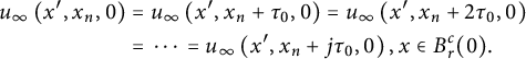 $$ \begin{align} \begin{aligned} u_{\infty}\left(x^{\prime}, x_n, 0\right) &=u_{\infty}\left(x^{\prime}, x_n+\tau_0, 0\right)=u_{\infty}\left(x^{\prime}, x_n+2 \tau_0, 0\right) \\ &=\cdots=u_{\infty}\left(x^{\prime}, x_n+j \tau_0, 0\right), x \in B_r^c(0). \end{aligned} \end{align} $$
Since the nth variable $\bar {x}_n^k$
of
$\bar {x}_n^k$
of $\bar {x}^k$
is bounded, we deduce from the asymptotic condition of (1.13) that
$\bar {x}^k$
is bounded, we deduce from the asymptotic condition of (1.13) that
 $$ \begin{align*}u_{\infty}\left(x^{\prime}, x_n, 0\right) \underset{x_n \rightarrow \pm \infty}{\longrightarrow} \pm 1 \text { uniformly in } x^{\prime}=\left(x_1, \ldots, x_{n-1}\right), \end{align*} $$
as a consequence, one can take $x_n$
sufficiently negative to let
$x_n$
sufficiently negative to let $u_{\infty }\left (x^{\prime }, x_n, 0\right )$
close to
$u_{\infty }\left (x^{\prime }, x_n, 0\right )$
close to $-1$
, and then take j sufficiently large to let
$-1$
, and then take j sufficiently large to let $u_{\infty }\left (x^{\prime }, x_n+j \tau _0, 0\right )$
close to 1, this is a contradiction with (3.15). Therefore, conclusion (3.8) must hold.
$u_{\infty }\left (x^{\prime }, x_n+j \tau _0, 0\right )$
close to 1, this is a contradiction with (3.15). Therefore, conclusion (3.8) must hold.
(II) Suppose $\tau _0>0$
, we are to show that there exists an
$\tau _0>0$
, we are to show that there exists an $\varepsilon>0$
such that
$\varepsilon>0$
such that
 $$ \begin{align} w_\tau(x, t) \leq 0, \,\,\,\forall(x, t) \in \mathbb{R}^{n-1} \times \mathbb{R}, \,\,\,\forall \tau \in\left(\tau_0-\varepsilon, \tau_0\right], \end{align} $$
which would contradict the definition of $\tau _0$
.
$\tau _0$
.
First, equation (3.8) implies that there exists a small constant $\varepsilon>0$
such that
$\varepsilon>0$
such that
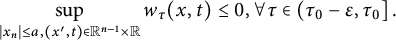 $$ \begin{align} \sup _{\left|x_n\right| \leq a,\left(x^{\prime}, t\right) \in \mathbb{R}^{n-1} \times \mathbb{R}} w_\tau(x, t) \leq 0, \forall \tau \in\left(\tau_0-\varepsilon, \tau_0\right]. \end{align} $$
Consequently, we only need to show that
 $$ \begin{align} \sup _{\left|x_n\right|>a,\left(x^{\prime}, t\right) \in \mathbb{R}^{n-1} \times \mathbb{R}} w_\tau(x, t) \leq 0, \forall \tau \in\left(\tau_0-\varepsilon, \tau_0\right]. \end{align} $$
In fact, if (3.18) is not valid, then there exists some $\tau \in \left (\tau _0-\varepsilon , \tau _0\right ]$
and a constant
$\tau \in \left (\tau _0-\varepsilon , \tau _0\right ]$
and a constant $A>0$
such that
$A>0$
such that
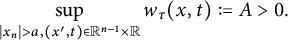 $$ \begin{align} \sup _{\left|x_n\right|>a,\left(x^{\prime}, t\right) \in \mathbb{R}^{n-1} \times \mathbb{R}} w_\tau(x, t):=A>0. \end{align} $$
Applying the asymptotic condition on u in (1.13), there exists a constant $M>a$
such that
$M>a$
such that
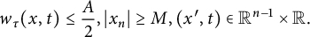 $$ \begin{align} w_\tau(x, t) \leq \frac{A}{2},\left|x_n\right| \geq M,\left(x^{\prime}, t\right) \in \mathbb{R}^{n-1} \times \mathbb{R}. \end{align} $$
To this end, we define
 $$ \begin{align*}E=\left\{\left(x^{\prime}, x_n, t\right) \in \mathbb{R}^{n-1} \times \mathbb{R} \times \mathbb{R}\Big| \,a<| x_n|<M,\left(x^{\prime}, t\right) \in \mathbb{R}^{n-1} \times \mathbb{R}\right\} \end{align*} $$
and consider the differential inequality in E satisfied by the function
 $$ \begin{align*}v_\tau(x, t):=w_\tau(x, t)-\frac{A}{2}. \end{align*} $$
For any $\tau \in \left (\tau _0-\varepsilon , \tau _0\right ],\left (x^{\prime }, t\right ) \in \mathbb {R}^{n-1} \times \mathbb {R}$
, if
$\tau \in \left (\tau _0-\varepsilon , \tau _0\right ],\left (x^{\prime }, t\right ) \in \mathbb {R}^{n-1} \times \mathbb {R}$
, if $a<x_n<M$
at the points in
$a<x_n<M$
at the points in $E \times \mathbb {R,}$
where
$E \times \mathbb {R,}$
where $v_\tau (x, t)>0$
, we have
$v_\tau (x, t)>0$
, we have
 $$ \begin{align*}u(x, t)>u_\tau(x, t)+\frac{A}{2} \geq u_\tau(x, t) \geq 1-\delta, \end{align*} $$
which implies
 $$ \begin{align} f(t, u(x, t))-f\left(t, u_\tau(x, t)\right) \leq 0, a<x_n<M,\left(x^{\prime}, t\right) \in \mathbb{R}^{n-1} \times \mathbb{R}. \end{align} $$
Another, using the monotonicity of f. If $-M<x_n<-a$
, at the points in
$-M<x_n<-a$
, at the points in $E \times \mathbb {R,}$
where
$E \times \mathbb {R,}$
where $v_\tau (x, t)>0$
, we have
$v_\tau (x, t)>0$
, we have
 $$ \begin{align*}u_\tau(x, t)<u(x, t)\leq -1+\delta. \end{align*} $$
Again with the assumption (1.14), one has
 $$ \begin{align} f(u(x, t))-f\left(u_\tau(x, t)\right) \leq 0,-M<x_n<-a,\left(x^{\prime}, t\right) \in \mathbb{R}^{n-1} \times \mathbb{R}. \end{align} $$
Therefore, in view of (3.21) and (3.22), at the points in $E \times \mathbb {R,}$
where
$E \times \mathbb {R,}$
where $v_\tau (x, t)>0$
, we have
$v_\tau (x, t)>0$
, we have
 $$ \begin{align*}\begin{aligned} \frac{\partial v_\tau}{\partial t}(x, t)-\left(\Delta+\lambda\right)^{\frac{\alpha}{2}} v_\tau(x, t) &=\frac{\partial u_\tau}{\partial t}(x, t)-\left(\Delta+\lambda\right)^{\frac{\alpha}{2}} u_\tau(x, t) \\ &=f(t, u(x, t))-f\left(t, u_\tau(x, t)\right) \leq 0. \end{aligned} \end{align*} $$
Noting by (3.17) and (3.20), we have the following exterior condition:
 $$ \begin{align*}v_\tau(x, t) \leq 0,(x, t) \in E^c \times \mathbb{R}, \end{align*} $$
which together with (3.18) and the maximum principle in unbounded domains Theorem 1.1, we obtain
 $$ \begin{align*}v_\tau(x, t) \leq 0,(x, t) \in \mathbb{R}^n \times \mathbb{R}, \forall \tau \in\left(\tau_0-\varepsilon, \tau_0\right]. \end{align*} $$
This contradicts the assumption (3.19), and it follows that (3.18) is valid, which also yield (3.7). Therefore, we complete the proof in Step 2.
Step 3. In this step, we will show that $u(x, t)$
is strictly increasing with respect to
$u(x, t)$
is strictly increasing with respect to $x_n$
, and
$x_n$
, and
 $$ \begin{align} u(x, t)=u\left(x_n, t\right). \end{align} $$
From Steps 1 and 2, we have derived that
 $$ \begin{align*}w_\tau(x, t) \leq 0,(x, t) \in \mathbb{R}^{n-1} \times \mathbb{R}, \,\,\forall \tau>0. \end{align*} $$
In order to show that $u(x, t)$
is strictly increasing with respect to
$u(x, t)$
is strictly increasing with respect to $x_n$
, we only need to show
$x_n$
, we only need to show
 $$ \begin{align} w_\tau(x, t)<0,(x, t) \in \mathbb{R}^{n-1} \times \mathbb{R}, \,\,\forall \tau>0. \end{align} $$
In fact, if equation (3.24) is not true, then there exists a point $\left (x^0, t_0\right ) \in \mathbb {R}^{n-1} \times \mathbb {R}$
and
$\left (x^0, t_0\right ) \in \mathbb {R}^{n-1} \times \mathbb {R}$
and $\tau _0>0$
such that
$\tau _0>0$
such that
 $$ \begin{align*}w_{\tau_0}\left(x^0, t_0\right)=0, \end{align*} $$
which means $\left (x^0, t_0\right )$
is a maximum point of
$\left (x^0, t_0\right )$
is a maximum point of $w_{\tau _0}(x, t)$
in
$w_{\tau _0}(x, t)$
in $\mathbb {R}^n \times \mathbb {R}$
, and
$\mathbb {R}^n \times \mathbb {R}$
, and
 $$ \begin{align*}\frac{\partial w_{\tau_0}}{\partial t}\left(x^0, t_0\right)=0. \end{align*} $$
Through a direct calculation, we have
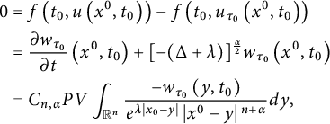 $$ \begin{align*}\begin{aligned} 0&=f\left(t_0, u\left(x^0, t_0\right)\right)-f\left(t_0, u_{\tau_0}\left(x^0, t_0\right)\right)\\ &=\frac{\partial w_{\tau_0}}{\partial t}\left(x^0, t_0\right)+[-(\Delta+\lambda)]^{\frac{\alpha}{2}} w_{\tau_0}\left(x^0, t_0\right) \\ &=C_{n, \alpha} P V \int_{\mathbb{R}^n} \frac{-w_{\tau_0}\left(y, t_0\right)}{e^{\lambda |x_0-y|}\left|x^0-y\right|{}^{n+\alpha}} d y, \end{aligned} \end{align*} $$
which implies immediately that
 $$ \begin{align*}w_{\tau_0}\left(y, t_0\right) \equiv 0,\,\,\, y \in \mathbb{R}^n. \end{align*} $$
Therefore, for any $j \in \mathbb {N}$
, we have
$j \in \mathbb {N}$
, we have
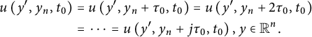 $$ \begin{align*}\begin{aligned} u\left(y^{\prime}, y_n, t_0\right) &=u\left(y^{\prime}, y_n+\tau_0, t_0\right)=u\left(y^{\prime}, y_n+2 \tau_0, t_0\right) \\ &=\cdots=u\left(y^{\prime}, y_n+j \tau_0, t_0\right), y \in \mathbb{R}^n. \end{aligned} \end{align*} $$
Recalling asymptotic condition, we can let $y_n$
sufficiently negative such that
$y_n$
sufficiently negative such that $u\left (y^{\prime }, y_n, t_0\right )$
is close to
$u\left (y^{\prime }, y_n, t_0\right )$
is close to $-1$
, and then take j sufficiently large such that
$-1$
, and then take j sufficiently large such that $u\left (x^{\prime }, x_n+j \tau _0, 0\right )$
is close to
$u\left (x^{\prime }, x_n+j \tau _0, 0\right )$
is close to $1$
; thus, we derive a contradiction and obtain (3.24), which yields that
$1$
; thus, we derive a contradiction and obtain (3.24), which yields that $u(x, t)$
is strictly increasing with respect to
$u(x, t)$
is strictly increasing with respect to $x_n$
.
$x_n$
.
Next, our goal is to prove that $u(x)$
depends on
$u(x)$
depends on $x_n$
only. Indeed, it can be seen from the above sliding procedure that the methods should still be valid if we replace
$x_n$
only. Indeed, it can be seen from the above sliding procedure that the methods should still be valid if we replace $u_\tau (x, t)$
by
$u_\tau (x, t)$
by $u(x+\tau \nu , t)$
with
$u(x+\tau \nu , t)$
with $\nu =\left (\nu _1, \ldots , \nu _n\right )$
and
$\nu =\left (\nu _1, \ldots , \nu _n\right )$
and $\nu _n>0$
. More accurately, applying similar sliding methods as in Steps 1 and 2, for each
$\nu _n>0$
. More accurately, applying similar sliding methods as in Steps 1 and 2, for each $\nu $
with
$\nu $
with $\nu _n>0$
, yields
$\nu _n>0$
, yields
 $$ \begin{align*}u(x+\tau \nu, t)>u(x, t), \forall \tau>0,(x, t) \in \mathbb{R}^{n-1} \times \mathbb{R}. \end{align*} $$
Let $\nu _n \rightarrow 0$
. We deduce from the continuity of
$\nu _n \rightarrow 0$
. We deduce from the continuity of $u(x, t)$
that
$u(x, t)$
that
 $$ \begin{align*}u(x+\tau \nu, t) \geq u(x, t) \end{align*} $$
for arbitrary $\nu $
with
$\nu $
with $\nu _n=0$
. Replacing
$\nu _n=0$
. Replacing $\nu $
by
$\nu $
by $-\nu $
, for arbitrary
$-\nu $
, for arbitrary $\nu $
with
$\nu $
with $\nu _n=0$
, we find that
$\nu _n=0$
, we find that
 $$ \begin{align*}u(x+\tau \nu, t) \leq u(x, t). \end{align*} $$
Therefore,
 $$ \begin{align*}u(x+\tau \nu, t)=u(x, t), \end{align*} $$
which indicates that $u\left (x^{\prime }, x_n, t\right )$
is independent of
$u\left (x^{\prime }, x_n, t\right )$
is independent of $x^{\prime }$
, hence (3.23) is true. Therefore, we have proved Step 3. This completes the proof of Theorem 1.2.
$x^{\prime }$
, hence (3.23) is true. Therefore, we have proved Step 3. This completes the proof of Theorem 1.2.
4 Monotonicity in epigraph E
In this section, combined the maximum principles Theorem 1.1 and sliding methods, we shall prove the monotonicity result on solutions to tempered fractional parabolic problem on epigraph E.
Proof For any $0<\tau <l$
, let
$0<\tau <l$
, let
 $$ \begin{align*}u^\tau(x,t):=u(x', x_n+\tau,t)\end{align*} $$
and
 $$ \begin{align*}w^\tau(x,t):=u(x,t)-u^\tau(x,t).\end{align*} $$
Since $f(\cdot )$
is non-increasing, we have
$f(\cdot )$
is non-increasing, we have
 $$ \begin{align*}\frac{\partial w^\tau}{\partial t}(x, t)-\left(\Delta+\lambda\right)^{\frac{\alpha}{2}}w^\tau(x,t)=f(u(x,t))-f(u^\tau(x,t))\leq 0 \end{align*} $$
at points $x\in E,$
where
$x\in E,$
where $w^\tau (x,t)<0$
. In addition, for any
$w^\tau (x,t)<0$
. In addition, for any $0<\tau <l$
, we have
$0<\tau <l$
, we have
 $$ \begin{align*}w^\tau(x,t)\leq 0, \quad \forall \,\, (x,t) \in \{\mathbb{R}^n\setminus E\}\times \mathbb R.\end{align*} $$
Thus, it follows immediately from Theorem 1.1 that, for any $0<\tau <l$
,
$0<\tau <l$
,
 $$ \begin{align*}w^\tau(x,t)\leq 0, \quad \forall \,\, (x,t)\in E\times \mathbb R.\end{align*} $$
Now, suppose that $u\not \equiv 0$
in
$u\not \equiv 0$
in $E\times \mathbb R$
, then there exists a
$E\times \mathbb R$
, then there exists a $(\hat {x},\hat {t})\in E\times \mathbb R$
such that
$(\hat {x},\hat {t})\in E\times \mathbb R$
such that $u(\hat {x},\hat {t})>0$
. We are to show that, for any
$u(\hat {x},\hat {t})>0$
. We are to show that, for any $0<\tau <l$
,
$0<\tau <l$
,
 $$ \begin{align} w^\tau(x,t)<0, \quad \forall \,\, x \in E\times\mathbb R. \end{align} $$
If not, there exists a point $(x^{\tau },t_0)\in E\times \mathbb R$
such that
$(x^{\tau },t_0)\in E\times \mathbb R$
such that
 $$ \begin{align*}w^\tau(x^{\tau},t_0)=0=\max_{\mathbb{R}^n\times \mathbb{R}}w^\tau(x,t), \end{align*} $$
and hence
 $$ \begin{align*}\frac{\partial w^\tau}{\partial t}(x^{\tau},t_0)=0. \end{align*} $$
One one hand, recalling the definition of $-\left (\Delta +\lambda \right )^{\frac {\alpha }{2}}$
, we know that
$-\left (\Delta +\lambda \right )^{\frac {\alpha }{2}}$
, we know that
 $$ \begin{align*}\frac{\partial w^\tau}{\partial t}(x^{\tau},t_0)-\left(\Delta+\lambda\right)^{\frac{\alpha}{2}}w^\tau(x^\tau,t_0)=C_{n, \alpha} P.V. \int_{\mathbb{R}^n} \frac{-w^{\tau}\left(y, t_0\right)}{e^{\lambda |x^\tau-y|}\left|x^\tau-y\right|{}^{n+\alpha}} d y>0. \end{align*} $$
On the other hand, one has
 $$ \begin{align*}\frac{\partial w^\tau}{\partial t}(x^{\tau},t_0)-\left(\Delta+\lambda\right)^{\frac{\alpha}{2}}w^\tau(x^\tau,t_0)= f(u(x^{\tau},t_0))-f(u^\tau(x^{\tau},t_0))=0. \end{align*} $$
That is impossible! Therefore, (4.1) holds; and hence, u is strictly monotone increasing in the $x_n$
direction. In particular,
$x_n$
direction. In particular, $u>0$
in E.
$u>0$
in E.
If, in addition, E is contained in a half-space, we will prove that
 $$ \begin{align*}u(x,t)\geq 0, \qquad \text{in}\,\,E\times \mathbb R,\end{align*} $$
and hence, the assumption (1.16) is redundant.
Without loss of generalities, we may assume that $E\subseteq \mathbb {R}^n_+$
, let
$E\subseteq \mathbb {R}^n_+$
, let
 $$ \begin{align} T_{0}:=\left\{x \in \mathbb{R}^{n} | x_n=0\right\}, \end{align} $$
 $$ \begin{align} \Sigma_{0}:=\left\{x \in \mathbb{R}^{n} | x_{n}>0\right\} \end{align} $$
be the region above the plane $T_0$
, and
$T_0$
, and
 $$ \begin{align*}x^{0}:=\left(x_{1}, x_{2}, \ldots, -x_{n}\right) \end{align*} $$
be the reflection of x about the plane $T_{0}$
. We denote
$T_{0}$
. We denote $u_{0}(x,t):=u\left (x^{0},t\right )$
and
$u_{0}(x,t):=u\left (x^{0},t\right )$
and $w_{0}(x,t)=u_{0}(x,t)-u(x,t)$
. For
$w_{0}(x,t)=u_{0}(x,t)-u(x,t)$
. For $(x,t)\in \Sigma _{0}\times \mathbb R,$
where
$(x,t)\in \Sigma _{0}\times \mathbb R,$
where $w_{0}(x,t)>0$
, we derive from (1.15) that, for any
$w_{0}(x,t)>0$
, we derive from (1.15) that, for any $(x,t)\in E\times \mathbb R,$
where
$(x,t)\in E\times \mathbb R,$
where $w_0(x,t)>0$
, one has
$w_0(x,t)>0$
, one has
 $$ \begin{align*} \frac{\partial w_0}{\partial t}(x,t)-\left(\Delta+\lambda\right)^{\frac{\alpha}{2}}w_0(x,t)= f(u_0(x,t))-f(u(x,t))\leq 0. \end{align*} $$
Hence, we obtain from theorem that $w_0\leq 0$
in
$w_0\leq 0$
in $\Sigma _{0}\times \mathbb R$
, which implies immediately
$\Sigma _{0}\times \mathbb R$
, which implies immediately $u\geq 0$
in
$u\geq 0$
in $E\times \mathbb R$
.
$E\times \mathbb R$
.
Furthermore, suppose E itself is exactly a half-space. Without loss of generalities, we may assume that $E=\mathbb {R}^n_+$
. We will show that
$E=\mathbb {R}^n_+$
. We will show that $u(x,t)$
depends on
$u(x,t)$
depends on $x_n$
only.
$x_n$
only.
In fact, when $E=\mathbb {R}^n_+$
, it can be seen from the above sliding procedure that the methods should still be valid if we replace
$E=\mathbb {R}^n_+$
, it can be seen from the above sliding procedure that the methods should still be valid if we replace $u^\tau (x,t):=u(x+\tau e_{n},t)$
by
$u^\tau (x,t):=u(x+\tau e_{n},t)$
by $u(x+\tau \nu ,t)$
, where
$u(x+\tau \nu ,t)$
, where $\nu =(\nu _1,\ldots ,\nu _n)$
is an arbitrary vector such that
$\nu =(\nu _1,\ldots ,\nu _n)$
is an arbitrary vector such that $\langle \nu ,e_{n}\rangle =\nu _{n}>0$
. Applying similar sliding methods as above, we can derive that, for arbitrary such vector
$\langle \nu ,e_{n}\rangle =\nu _{n}>0$
. Applying similar sliding methods as above, we can derive that, for arbitrary such vector $\nu $
,
$\nu $
,
 $$ \begin{align*}u(x+\tau\nu,t)>u(x,t) \quad \text{in} \,\, \mathbb{R}^n_+\times\mathbb R, \quad \forall \,\, \tau>0.\end{align*} $$
Let $\nu _n\rightarrow 0+$
, from the continuity of u, we deduce that
$\nu _n\rightarrow 0+$
, from the continuity of u, we deduce that
 $$ \begin{align*}u(x+\tau\nu,t)\geq u(x,t)\end{align*} $$
for arbitrary vector $\nu $
with
$\nu $
with $\nu _n=0$
. By replacing
$\nu _n=0$
. By replacing $\nu $
by
$\nu $
by $-\nu $
, we arrive at
$-\nu $
, we arrive at
 $$ \begin{align*}u(x+\tau\nu,t)=u(x,t)\end{align*} $$
for arbitrary vector $\nu $
with
$\nu $
with $\nu _n=0$
, this means that
$\nu _n=0$
, this means that $u(x,t)$
is independent of
$u(x,t)$
is independent of $x'$
, hence
$x'$
, hence $u(x,t)=u(x_n,t)$
. This finishes the proof of Theorem 1.4.
$u(x,t)=u(x_n,t)$
. This finishes the proof of Theorem 1.4.
Acknowledgment
The author is grateful to the anonymous referees for their careful reading and valuable comments and suggestions that improved the presentation of the article.
Data availability statement
My manuscript has no associated data.


