


1. Introduction
A Hamilton cycle in a graph is a cycle that passes through all the vertices of the graph exactly once, and a graph containing a Hamilton cycle is called Hamiltonian. Even though a Hamilton cycle is a relatively simple structure, determining whether a certain graph is Hamiltonian was included in the list of $21$
NP-hard problems by Karp [Reference Karp21]. Thus, there is significant interest in deriving conditions that ensure Hamiltonicity in a given graph. For instance, the celebrated Dirac’s theorem [Reference Dirac9] states that every graph on
$21$
NP-hard problems by Karp [Reference Karp21]. Thus, there is significant interest in deriving conditions that ensure Hamiltonicity in a given graph. For instance, the celebrated Dirac’s theorem [Reference Dirac9] states that every graph on $n \geq 3$
vertices with a minimum degree of
$n \geq 3$
vertices with a minimum degree of $n/2$
is Hamiltonian. For more results on Hamiltonicity, readers can refer to the surveys [Reference Frieze12, Reference Kühn and Osthus27, Reference Kühn and Osthus28].
$n/2$
is Hamiltonian. For more results on Hamiltonicity, readers can refer to the surveys [Reference Frieze12, Reference Kühn and Osthus27, Reference Kühn and Osthus28].
Most classical sufficient conditions for a graph to be Hamiltonian are only applicable to relatively dense graphs, such as those considered in Dirac’s Theorem. Establishing sufficient conditions for Hamiltonicity in sparse graphs is known to be much more challenging. Sparse random graphs are natural objects to consider as starting points, and they have attracted a lot of attention in the past few decades. In 1976, Pósa [Reference Pósa34] proved that for some large constant $C$
, the binomial random graph model
$C$
, the binomial random graph model $G(n, p)$
with
$G(n, p)$
with $p \geq C\log n/n$
is typically Hamiltonian. In the following few years, Korshunov [Reference Korshunov24] refined Pósa’s result, and in 1983, Bollobás [Reference Bollobás5], and independently Komlós and Szemerédi [Reference Komlós and Szemerédi23] showed a more precise threshold for Hamiltonicity. Their results demonstrate that if
$p \geq C\log n/n$
is typically Hamiltonian. In the following few years, Korshunov [Reference Korshunov24] refined Pósa’s result, and in 1983, Bollobás [Reference Bollobás5], and independently Komlós and Szemerédi [Reference Komlós and Szemerédi23] showed a more precise threshold for Hamiltonicity. Their results demonstrate that if $p = (\log n + \log \log n + \omega (1))/n$
, then the probability of the random graph
$p = (\log n + \log \log n + \omega (1))/n$
, then the probability of the random graph $G(n, p)$
being Hamiltonian tends to 1 (we say such an event happens with high probability, or whp for brevity).
$G(n, p)$
being Hamiltonian tends to 1 (we say such an event happens with high probability, or whp for brevity).
Following the fruitful study of random graphs, it is natural to explore families of deterministic graphs that behave in some ways like random graphs; these are sometimes called pseudorandom graphs. A natural candidate to begin with is the following: suppose that we sample a random graph $G\sim G(n,p)$
, and then allow an adversary to delete a constant fraction of the edges incident to each vertex. The resulting subgraph
$G\sim G(n,p)$
, and then allow an adversary to delete a constant fraction of the edges incident to each vertex. The resulting subgraph $H\subseteq G$
loses all its randomness. Thus, we cannot use, for example, a multiple exposure trick and concentration inequalities, which were heavily used in the proof of Hamiltonicity of a typical
$H\subseteq G$
loses all its randomness. Thus, we cannot use, for example, a multiple exposure trick and concentration inequalities, which were heavily used in the proof of Hamiltonicity of a typical $G\sim G(n,p)$
. Under such a model, one of the central problems to consider is quantifying the local resilience of the random graph
$G\sim G(n,p)$
. Under such a model, one of the central problems to consider is quantifying the local resilience of the random graph $G$
with respect to Hamiltonicity. In [Reference Sudakov and Vu36], Sudakov and Vu initiated the study of local resilience of random graphs, and they showed that for any
$G$
with respect to Hamiltonicity. In [Reference Sudakov and Vu36], Sudakov and Vu initiated the study of local resilience of random graphs, and they showed that for any ${\varepsilon } \gt 0$
, if
${\varepsilon } \gt 0$
, if $p$
is somewhat greater than
$p$
is somewhat greater than $\log ^4n/n$
, then
$\log ^4n/n$
, then $G(n, p)$
typically has the property that every spanning subgraph with a minimum degree of at least
$G(n, p)$
typically has the property that every spanning subgraph with a minimum degree of at least $(1 + {\varepsilon })np/2$
contains a Hamilton cycle. They also conjectured that this remains true as long as
$(1 + {\varepsilon })np/2$
contains a Hamilton cycle. They also conjectured that this remains true as long as $p=(\log n+\omega (1))/n$
, which was solved by Lee and Sudakov [Reference Lee and Sudakov29]. Later, an even stronger result, the so-called “hitting-time” statement, was shown by Nenadov, Steger and Trujić [Reference Nenadov, Steger and Trujić32], and Montgomery [Reference Montgomery30], independently.
$p=(\log n+\omega (1))/n$
, which was solved by Lee and Sudakov [Reference Lee and Sudakov29]. Later, an even stronger result, the so-called “hitting-time” statement, was shown by Nenadov, Steger and Trujić [Reference Nenadov, Steger and Trujić32], and Montgomery [Reference Montgomery30], independently.
Exploring the properties of pseudorandom graphs, which has attracted many researchers in the area, is much more challenging than studying random graphs. The first quantitative notion of pseudorandom graphs was introduced by Thomason [Reference Thomason37, Reference Thomason38]. He initiated the study of pseudorandom graphs by introducing the so-called $(p,\lambda )$
-jumbled graphs, which satisfy
$(p,\lambda )$
-jumbled graphs, which satisfy $|e(U)-p\binom {|U|}{2}|\leq \lambda |U|$
for every vertex subset
$|e(U)-p\binom {|U|}{2}|\leq \lambda |U|$
for every vertex subset $U\subseteq V$
. Since then, there has been a great deal of investigation into different types and various properties of pseudorandom graphs, for example, [Reference Allen, Böttcher, Hàn, Kohayakawa and Person1, Reference Conlon, Fox and Zhao8, Reference Hàn, Han and Morris15, Reference Han, Kohayakawa, Morris and Person16, Reference Kohayakawa, Rödl, Schacht, Sissokho and Skokan22, Reference Nenadov31]. This remains a very active area of research in graph theory.
$U\subseteq V$
. Since then, there has been a great deal of investigation into different types and various properties of pseudorandom graphs, for example, [Reference Allen, Böttcher, Hàn, Kohayakawa and Person1, Reference Conlon, Fox and Zhao8, Reference Hàn, Han and Morris15, Reference Han, Kohayakawa, Morris and Person16, Reference Kohayakawa, Rödl, Schacht, Sissokho and Skokan22, Reference Nenadov31]. This remains a very active area of research in graph theory.
One special class of pseudorandom graphs which has been studied extensively is the class of spectral expander graphs, also known as $(n,d,\lambda )$
-graphs. Given a graph
$(n,d,\lambda )$
-graphs. Given a graph $G$
on vertex set
$G$
on vertex set $V=\{v_1,\ldots, v_n\}$
, its adjacency matrix
$V=\{v_1,\ldots, v_n\}$
, its adjacency matrix $A\,:\!=\,A(G)$
is an
$A\,:\!=\,A(G)$
is an $n\times n$
,
$n\times n$
, $0/1$
matrix, defined by
$0/1$
matrix, defined by $A_{ij}=1$
if and only if
$A_{ij}=1$
if and only if $v_iv_j\in E(G)$
. Let
$v_iv_j\in E(G)$
. Let $s_1(A)\geq s_2(A)\geq \cdots \geq s_n(A)$
be the singular values of
$s_1(A)\geq s_2(A)\geq \cdots \geq s_n(A)$
be the singular values of $A$
(see Definition 3.3). Observe that for a
$A$
(see Definition 3.3). Observe that for a $d$
-regular graph
$d$
-regular graph $G$
, we always have
$G$
, we always have $s_1(G)\,:\!=\,s_1(A(G))=d$
, so the largest singular value is not a very interesting quantity. We say that
$s_1(G)\,:\!=\,s_1(A(G))=d$
, so the largest singular value is not a very interesting quantity. We say that $G$
is an
$G$
is an $(n,d,\lambda )$
-graph if it is a
$(n,d,\lambda )$
-graph if it is a $d$
-regular graph on
$d$
-regular graph on $n$
vertices with
$n$
vertices with $s_2(G) \leq \lambda$
.
$s_2(G) \leq \lambda$
.
The celebrated Expander Mixing Lemma (see, e.g. Chapter 9 in [Reference Alon and Spencer3]) provides a powerful formula to estimate the edge distribution of an $(n, d, \lambda )$
-graph, which suggests that
$(n, d, \lambda )$
-graph, which suggests that $(n,d,\lambda )$
-graphs are indeed special cases of jumbled graphs, and that
$(n,d,\lambda )$
-graphs are indeed special cases of jumbled graphs, and that $G$
has stronger expansion properties for smaller values of
$G$
has stronger expansion properties for smaller values of $\lambda$
. Thus, it is natural to seek for the best possible condition on the spectral gap (defined as the ratio
$\lambda$
. Thus, it is natural to seek for the best possible condition on the spectral gap (defined as the ratio $\lambda /d$
) which guarantees certain properties. Examples of such results can be found e.g. in [Reference Alon, Krivelevich and Sudakov2, Reference Balogh, Csaba, Pei and Samotij4, Reference Han and Yang17, Reference Pavez-Signé33]. For more on
$\lambda /d$
) which guarantees certain properties. Examples of such results can be found e.g. in [Reference Alon, Krivelevich and Sudakov2, Reference Balogh, Csaba, Pei and Samotij4, Reference Han and Yang17, Reference Pavez-Signé33]. For more on $(n,d,\lambda )$
-graphs and their many applications, we refer the reader to the surveys of Hoory, Linial and Wigderson [Reference Hoory, Linial and Wigderson19], Krivelevich and Sudakov [Reference Krivelevich and Sudakov26], the book of Brouwer and Haemers [Reference Brouwer and Haemers6], and the references therein.
$(n,d,\lambda )$
-graphs and their many applications, we refer the reader to the surveys of Hoory, Linial and Wigderson [Reference Hoory, Linial and Wigderson19], Krivelevich and Sudakov [Reference Krivelevich and Sudakov26], the book of Brouwer and Haemers [Reference Brouwer and Haemers6], and the references therein.
Hamiltonicity of $(n,d,\lambda )$
-graphs was first studied by Krivelevich and Sudakov [Reference Krivelevich and Sudakov25], who proved a sufficient condition on the spectral gap forcing Hamiltonicity. More precisely, they showed that for sufficiently large
$(n,d,\lambda )$
-graphs was first studied by Krivelevich and Sudakov [Reference Krivelevich and Sudakov25], who proved a sufficient condition on the spectral gap forcing Hamiltonicity. More precisely, they showed that for sufficiently large $n$
, any
$n$
, any $(n,d,\lambda )$
-graph with
$(n,d,\lambda )$
-graph with
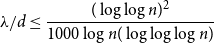 \begin{equation*} \lambda /d\leq \frac {(\log \log n)^2}{1000\log n(\log \log \log n)} \end{equation*}
has a Hamilton cycle. In the same paper, Krivelevich and Sudakov made the following conjecture.
Conjecture 1.1.
There exists an absolute constant $c \gt 0$
such that for any sufficiently large integer
$c \gt 0$
such that for any sufficiently large integer $n$
, any
$n$
, any $(n,d,\lambda )$
-graph with
$(n,d,\lambda )$
-graph with $\lambda /d\leq c$
contains a Hamilton cycle.
$\lambda /d\leq c$
contains a Hamilton cycle.
Although there are numerous related results in this direction, there had been no improvement on the original bound until the recent result given by Glock, Correia, and Sudakov [Reference Glock, Correia and Sudakov14]. In their paper, they improved the above result in two different ways: $(i)$
they demonstrated that the spectral gap
$(i)$
they demonstrated that the spectral gap $\lambda /d\leq c/(\log n)^{1/3}$
already guarantees Hamiltonicity;
$\lambda /d\leq c/(\log n)^{1/3}$
already guarantees Hamiltonicity; $(ii)$
they confirmed Conjecture 1.1 in the case where
$(ii)$
they confirmed Conjecture 1.1 in the case where $d\geq n^{\alpha }$
for every fixed constant
$d\geq n^{\alpha }$
for every fixed constant $\alpha \gt 0$
.
$\alpha \gt 0$
.
In this paper, we improve the second result in [Reference Glock, Correia and Sudakov14].
Theorem 1.2.
There exists an absolute constant $c \gt 0$
such that for any sufficiently large integer
$c \gt 0$
such that for any sufficiently large integer $n$
, any
$n$
, any $(n,d,\lambda )$
-graph with
$(n,d,\lambda )$
-graph with $\lambda /d\leq c$
and
$\lambda /d\leq c$
and $d \geq \log ^{6}n$
contains a Hamilton cycle.
$d \geq \log ^{6}n$
contains a Hamilton cycle.
Our proof works for $c=\frac {1}{70000}$
, although we made no attempt to optimize this constant.
$c=\frac {1}{70000}$
, although we made no attempt to optimize this constant.
It is worth mentioning that Draganić, Montgomery, Correia, Pokrovskiy, and Sudakov independently verified Conjecture 1.1 in [Reference Draganić, Montgomery, Correia, Pokrovskiy and Sudakov10], and in particular, they proved a stronger statement than our main result. Their approach relies on extensions of the Pósa rotation-extension technique and sorting networks, and utilizes a result in [Reference Hyde, Morrison, Müyesser and Pavez-Signé20] to obtain a linking structure. In contrast, while our work utilizes a previous result on closing vertex-disjoint paths into a cycle, it is primarily based on new machinery introduced in this paper, as summarized in Theorem6.2. Specifically, we show that the spectral gap of a random induced subgraph of an $(n,d,\lambda )$
-graph is typically bounded above by the spectral gap of the original graph, up to a constant factor.
$(n,d,\lambda )$
-graph is typically bounded above by the spectral gap of the original graph, up to a constant factor.
To achieve this, we utilize results on norms of principal submatrices, such as the Rudelson–Vershynin Theorem [Reference Rudelson and Vershynin35] (see Section 6), and demonstrate that, with probability $1 - n^{-\Theta (1)}$
, the spectral gap of the induced subgraph remains
$1 - n^{-\Theta (1)}$
, the spectral gap of the induced subgraph remains $O(\lambda /d)$
for a sufficiently large random vertex subset. We believe that this result will have further applications.
$O(\lambda /d)$
for a sufficiently large random vertex subset. We believe that this result will have further applications.
The paper is organized as follows. In Section 2, we provide an outline of the proof. Section 3 contains the proof of the expander mixing lemma for matrices, followed by an analysis of the special case for almost $(n,d,\lambda )$
-graphs in Section 4. In Section 5, we introduce the extendability property and reference a useful result from [Reference Hyde, Morrison, Müyesser and Pavez-Signé20], which ensures that vertex-disjoint paths can be used to connect designated pairs of vertices in
$(n,d,\lambda )$
-graphs in Section 4. In Section 5, we introduce the extendability property and reference a useful result from [Reference Hyde, Morrison, Müyesser and Pavez-Signé20], which ensures that vertex-disjoint paths can be used to connect designated pairs of vertices in $(n,d,\lambda )$
-graphs. Our key lemma, which concerns the second singular value of a random-induced subgraph of an
$(n,d,\lambda )$
-graphs. Our key lemma, which concerns the second singular value of a random-induced subgraph of an $(n,d,\lambda )$
-graph, is presented in Section 6. Finally, in Section 7, we prove our main result, Theorem1.2, along with a generalized version, Theorem7.1, for “almost”
$(n,d,\lambda )$
-graph, is presented in Section 6. Finally, in Section 7, we prove our main result, Theorem1.2, along with a generalized version, Theorem7.1, for “almost” $(n,d,\lambda )$
-graphs. For the reader’s convenience, we also include some standard tools from linear algebra and several technical proofs in the Appendix.
$(n,d,\lambda )$
-graphs. For the reader’s convenience, we also include some standard tools from linear algebra and several technical proofs in the Appendix.
1.1 Notation
For a graph $G=(V,E)$
, let
$G=(V,E)$
, let $e(G)\,:\!=\,|E(G)|$
. We mostly assume that
$e(G)\,:\!=\,|E(G)|$
. We mostly assume that $V=[n]$
for simplicity. For a subset
$V=[n]$
for simplicity. For a subset $A\subseteq V$
of size
$A\subseteq V$
of size $m$
, we simply call it an
$m$
, we simply call it an $m$
-set, and we denote the family of all
$m$
-set, and we denote the family of all $m$
-sets of
$m$
-sets of $V$
by
$V$
by $\binom {V}{m}$
. For two vertex sets
$\binom {V}{m}$
. For two vertex sets $A, B \subseteq V (G)$
, we define
$A, B \subseteq V (G)$
, we define $E_G(A,B)$
to be the set of all edges
$E_G(A,B)$
to be the set of all edges $xy\in E(G)$
with
$xy\in E(G)$
with $x\in A$
and
$x\in A$
and $y\in B$
, and set
$y\in B$
, and set $e_G(A,B)\,:\!=\,|E_G(A,B)|$
. For two disjoint subsets
$e_G(A,B)\,:\!=\,|E_G(A,B)|$
. For two disjoint subsets $X,Y\subseteq V$
, we write
$X,Y\subseteq V$
, we write $G[X,Y]$
to denote the induced bipartite subgraph of
$G[X,Y]$
to denote the induced bipartite subgraph of $G$
with parts
$G$
with parts $X$
and
$X$
and $Y$
. Moreover, we define
$Y$
. Moreover, we define $N_G(v)$
to be the neighbourhood of a vertex
$N_G(v)$
to be the neighbourhood of a vertex $v$
, and define
$v$
, and define $N_G(A) \,:\!=\, \bigcup _{v\in A} N_G(v) \setminus A$
for a subset
$N_G(A) \,:\!=\, \bigcup _{v\in A} N_G(v) \setminus A$
for a subset $A\subseteq V$
. We write
$A\subseteq V$
. We write $N_G(A, B) = N_G(A) \cap B$
and for a vertex
$N_G(A, B) = N_G(A) \cap B$
and for a vertex $v$
, let
$v$
, let $N_G(v, B) = N_G(v) \cap B$
. We also write
$N_G(v, B) = N_G(v) \cap B$
. We also write $\deg _G(v)\,:\!=\,|N_G(v)|$
and
$\deg _G(v)\,:\!=\,|N_G(v)|$
and $\deg _G(v,B)\,:\!=\,|N_G(v,B)|$
. Finally, let
$\deg _G(v,B)\,:\!=\,|N_G(v,B)|$
. Finally, let $\delta (G)$
be the minimum degree of
$\delta (G)$
be the minimum degree of $G$
and let
$G$
and let $\Delta (G)$
be the maximum degree of
$\Delta (G)$
be the maximum degree of $G$
.
$G$
.
The adjacency matrix of $G$
, denoted by
$G$
, denoted by $A\,:\!=\,A(G)$
, is a
$A\,:\!=\,A(G)$
, is a $0/1$
,
$0/1$
, $n\times n$
matrix such that
$n\times n$
matrix such that $A_{i,j}=1$
if and only if
$A_{i,j}=1$
if and only if $ij\in E(G)$
. Moreover, given any subset
$ij\in E(G)$
. Moreover, given any subset $X\subseteq V$
, its characteristic vector
$X\subseteq V$
, its characteristic vector $\unicode {x1D7D9}_X\in \mathbb {R}^n$
is defined by
$\unicode {x1D7D9}_X\in \mathbb {R}^n$
is defined by
 \begin{equation*}\unicode {x1D7D9}_X(i)=\begin{cases} 1 &\textrm { if } i\in X\\ 0 &\textrm { otherwise} \end{cases}.\end{equation*}
We will often omit the subscript to ease the notation, unless otherwise stated. Since all of our calculations are asymptotic, we will often omit floor and ceiling functions whenever they are not crucial.
2. Proof outline
Our strategy for finding a Hamilton cycle in an $(n,d,\lambda )$
-graph
$(n,d,\lambda )$
-graph $G$
consists of two main phases. First, taking two disjoint vertex subsets
$G$
consists of two main phases. First, taking two disjoint vertex subsets $X,Y\subseteq V(G)$
of the same size
$X,Y\subseteq V(G)$
of the same size $\Theta (n/\log ^4n)$
, we find a subgraph
$\Theta (n/\log ^4n)$
, we find a subgraph $S_{res}\subseteq G$
with
$S_{res}\subseteq G$
with $|V(S_{res})|=\Theta (n/\log n)$
covering
$|V(S_{res})|=\Theta (n/\log n)$
covering $X$
and
$X$
and $Y$
, using a recent result (see Lemma 5.3 later) of Hyde, Morrison, M FC;yesser and Pavez-Signé [Reference Hyde, Morrison, Müyesser and Pavez-Signé20]. This subgraph includes various path factors for later use, where each path has one endpoint in
$Y$
, using a recent result (see Lemma 5.3 later) of Hyde, Morrison, M FC;yesser and Pavez-Signé [Reference Hyde, Morrison, Müyesser and Pavez-Signé20]. This subgraph includes various path factors for later use, where each path has one endpoint in $X$
and the other in
$X$
and the other in $Y$
. Then, we cover
$Y$
. Then, we cover $V(G)\setminus (V(S_{res})\setminus (X\cup Y))$
by vertex-disjoint paths, with one endpoint in
$V(G)\setminus (V(S_{res})\setminus (X\cup Y))$
by vertex-disjoint paths, with one endpoint in $X$
and the other in
$X$
and the other in $Y$
. Now, we are allowed to close the paths into a cycle by using one path factor in the prepared subgraph
$Y$
. Now, we are allowed to close the paths into a cycle by using one path factor in the prepared subgraph $S_{res}$
. Since all the vertices are used and passed through exactly once, the cycle is indeed a Hamilton cycle.
$S_{res}$
. Since all the vertices are used and passed through exactly once, the cycle is indeed a Hamilton cycle.
We now explain our method thoroughly. First, we take two random disjoint subsets $X,Y\subseteq V(G)$
of equal size
$X,Y\subseteq V(G)$
of equal size $\Theta (n/\log ^4 n)$
. Using Proposition 5.2, we can deduce that whp, the empty graph
$\Theta (n/\log ^4 n)$
. Using Proposition 5.2, we can deduce that whp, the empty graph $I(X\cup Y)$
is “extendable” (see Definition 5.1), which further produces a crucial subgraph
$I(X\cup Y)$
is “extendable” (see Definition 5.1), which further produces a crucial subgraph $S_{res}\subseteq G$
on
$S_{res}\subseteq G$
on $\Theta (n/\log n)$
vertices such that
$\Theta (n/\log n)$
vertices such that $X\cup Y\subseteq V(S_{res})$
(see Lemma 5.3). The powerful property of
$X\cup Y\subseteq V(S_{res})$
(see Lemma 5.3). The powerful property of $S_{res}$
that we will use is the following: for any ordering of the pairs in
$S_{res}$
that we will use is the following: for any ordering of the pairs in $(X,Y)$
, there exists a path factor in
$(X,Y)$
, there exists a path factor in $S_{res}$
connecting such pairs. This property will be used to connect the paths with endpoints in
$S_{res}$
connecting such pairs. This property will be used to connect the paths with endpoints in $X$
and
$X$
and $Y$
obtained in the second phase.
$Y$
obtained in the second phase.
Next, since $|V(S_{res})|=\Theta (n/\log n)$
, we can utilize its randomness in a way so that after removing it, the graph is still pseudorandom. Thus, by randomly partitioning
$|V(S_{res})|=\Theta (n/\log n)$
, we can utilize its randomness in a way so that after removing it, the graph is still pseudorandom. Thus, by randomly partitioning $V(G)\setminus V(S_{res})$
into
$V(G)\setminus V(S_{res})$
into $|X|$
-sets, if we can find a perfect matching between each two consecutive parts, we will obtain the desired vertex-disjoint paths
$|X|$
-sets, if we can find a perfect matching between each two consecutive parts, we will obtain the desired vertex-disjoint paths $P_i$
connecting
$P_i$
connecting $x_i\in X$
and
$x_i\in X$
and $y_i\in Y$
. Now, using the path factor in
$y_i\in Y$
. Now, using the path factor in $S_{res}$
connecting
$S_{res}$
connecting $(x_i,y_i)$
s, we can concatenate all the paths
$(x_i,y_i)$
s, we can concatenate all the paths $P_i$
into a cycle.
$P_i$
into a cycle.
It remains to ensure, whp, perfect matchings between two random disjoint subsets in an expander graph. To prove this, we demonstrate that the bipartite subgraph induced by each two consecutive parts is a good expander. Equivalently, it suffices to study the spectral properties of random induced subgraphs of $G$
, and this is the main contribution of this paper. It is crucial to remark that although there are some previous results on randomly selecting edges, e.g. [Reference Chung and Horn7], we randomly pick vertex subsets instead of picking edges. Using results on norms of principal matrices, e.g. Rudelson-Vershynin theorem in [Reference Rudelson and Vershynin35], we show that with probability at least
$G$
, and this is the main contribution of this paper. It is crucial to remark that although there are some previous results on randomly selecting edges, e.g. [Reference Chung and Horn7], we randomly pick vertex subsets instead of picking edges. Using results on norms of principal matrices, e.g. Rudelson-Vershynin theorem in [Reference Rudelson and Vershynin35], we show that with probability at least $1-n^{-\Theta (1)}$
, the spectral gap of a random induced subgraph of
$1-n^{-\Theta (1)}$
, the spectral gap of a random induced subgraph of $(n,d,\lambda )$
-graph is still
$(n,d,\lambda )$
-graph is still $O(\lambda /d)$
(see Theorem6.2).
$O(\lambda /d)$
(see Theorem6.2).
3. Expander mixing lemma for matrices
One of the most useful tools in spectral graph theory is the expander mixing lemma, which asserts that an $(n,d,\lambda )$
-graph is an expander (see, e.g., [Reference Hoory, Linial and Wigderson19]).
$(n,d,\lambda )$
-graph is an expander (see, e.g., [Reference Hoory, Linial and Wigderson19]).
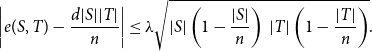
Theorem 3.1 (Expander mixing lemma). Let $G=(V,E)$
be an
$G=(V,E)$
be an $(n,d,\lambda )$
-graph. Then, for any two subsets
$(n,d,\lambda )$
-graph. Then, for any two subsets $S,T\subseteq V$
, we have
$S,T\subseteq V$
, we have
 \begin{equation*} \left |e(S,T)-\frac {d|S||T|}{n}\right | \leq \lambda \sqrt {|S| \left ( 1-\frac {|S|}{n} \right ) \, |T| \left ( 1-\frac {|T|}{n} \right )}. \end{equation*}
We will need a more general version of the expander mixing lemma which can be applied to non-regular graphs, digraphs, and even to general $m \times n$
matrices
$m \times n$
matrices $A$
. To state such a general result, it is convenient to normalize
$A$
. To state such a general result, it is convenient to normalize $A$
in the following way:
$A$
in the following way:
Definition 3.2 (Normalized matrix). Let $A$
be an
$A$
be an $m\times n$
matrix. Let
$m\times n$
matrix. Let $L=L(A)$
be the
$L=L(A)$
be the $m\times m$
diagonal matrix with
$m\times m$
diagonal matrix with $L_{i,i}=\sum _{j}A_{i,j}$
for all
$L_{i,i}=\sum _{j}A_{i,j}$
for all $i$
(that is, the sum of entries in the
$i$
(that is, the sum of entries in the $i$
th row), and
$i$
th row), and $R=R(A)$
be the
$R=R(A)$
be the $n\times n$
diagonal matrix with
$n\times n$
diagonal matrix with $R_{j,j}=\sum _{i}A_{i,j}$
(that is, the sum of entries in the
$R_{j,j}=\sum _{i}A_{i,j}$
(that is, the sum of entries in the $j$
th column). The normalized matrix of the matrix
$j$
th column). The normalized matrix of the matrix $A$
is defined as
$A$
is defined as
 \begin{equation*} \bar {A}\,:\!=\,L^{-1/2}AR^{-1/2}. \end{equation*}
In particular, if $A$
is a symmetric
$A$
is a symmetric $n \times n$
matrix, then the diagonal matrix
$n \times n$
matrix, then the diagonal matrix $L(A)=R(A)=: D(A)$
is called the degree matrix of
$L(A)=R(A)=: D(A)$
is called the degree matrix of $A$
.
$A$
.
Since the notion of eigenvalues is undefined for non-square matrices, it would be convenient for us to work with singular values which are defined as follows for all matrices.
Definition 3.3 (Singular values). Let $A$
be a real
$A$
be a real $m\times n$
matrix. The singular values of
$m\times n$
matrix. The singular values of $A$
are the nonnegative square roots of the eigenvalues of the symmetric positive semidefinite matrix
$A$
are the nonnegative square roots of the eigenvalues of the symmetric positive semidefinite matrix $A^{\mathsf {T}} A$
. We will always assume that
$A^{\mathsf {T}} A$
. We will always assume that $s_k(A)$
is the
$s_k(A)$
is the $k$
th singular value of
$k$
th singular value of $A$
in nonincreasing order. In particular, the singular values and the eigenvalues of a symmetric positive semidefinite matrix
$A$
in nonincreasing order. In particular, the singular values and the eigenvalues of a symmetric positive semidefinite matrix $A$
coincide.
$A$
coincide.
We are now ready to state a more general version of the expander mixing lemma.
Theorem 3.4 (Expander mixing lemma for matrices). Let $A$
be an
$A$
be an $m\times n$
matrix with nonnegative entries, and let
$m\times n$
matrix with nonnegative entries, and let $\bar {A}$
be the normalized matrix of
$\bar {A}$
be the normalized matrix of $A$
. Then, for any two subsets
$A$
. Then, for any two subsets $S\subseteq [m]$
and
$S\subseteq [m]$
and $T\subseteq [n]$
, we have
$T\subseteq [n]$
, we have
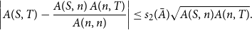
 \begin{equation*}\left |A(S,T)-\frac {A(S,n) \, A(m,T)}{A(m,n)}\right | \leq s_2(\bar {A})\sqrt {A(S,n)\left (1-\frac {A(S,n)}{A(m,n)}\right ) \, A(m,T) \left (1-\frac {A(m,T)}{A(m,n)}\right )},\end{equation*}
where we adopt the notation $A(S,T) \,:\!=\, \sum _{i \in S, j \in T} A_{i,j}$
, and we abbreviate
$A(S,T) \,:\!=\, \sum _{i \in S, j \in T} A_{i,j}$
, and we abbreviate $A(S,n) \,:\!=\, A(S,[n])$
,
$A(S,n) \,:\!=\, A(S,[n])$
, $A(m,T) \,:\!=\, A([m],T)$
, and
$A(m,T) \,:\!=\, A([m],T)$
, and $A(m,n) \,:\!=\, A([m],[n])$
.
$A(m,n) \,:\!=\, A([m],[n])$
.
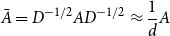
Observe that Theorem3.4 trivially implies Theorem3.1, since the adjacency matrix of a $d$
-regular graph satisfies
$d$
-regular graph satisfies
 \begin{equation*} \bar {A}=\frac {1}{d}A. \end{equation*}
The proof of Theorem3.4 is almost identical to the standard proof of Theorem3.1 that can be found e.g. as Proposition 4.3.2 in [Reference Brouwer and Haemers6]. Since we could not find a reference for this specific statement and its proof, we include the proof of Theorem3.4 for the convenience of the reader, without claiming any originality. It is based on the following crucial observation.
Observation 3.5.
Let $A$
be an
$A$
be an $m \times n$
matrix with nonnegative entries. Let
$m \times n$
matrix with nonnegative entries. Let $a \,:\!=\, A(m,n)$
and let
$a \,:\!=\, A(m,n)$
and let $\unicode {x1D7D9}_n$
denote the vector in
$\unicode {x1D7D9}_n$
denote the vector in ${\mathbb {R}}^n$
whose all coordinates are equal to
${\mathbb {R}}^n$
whose all coordinates are equal to $1$
. Consider the vectors
$1$
. Consider the vectors $\mathbf {u}_1 \,:\!=\, a^{-1/2} L^{1/2} \unicode {x1D7D9}_m$
and
$\mathbf {u}_1 \,:\!=\, a^{-1/2} L^{1/2} \unicode {x1D7D9}_m$
and ${\mathbf {v}}_1 \,:\!=\, a^{-1/2} R^{1/2} \unicode {x1D7D9}_n$
. Then:
${\mathbf {v}}_1 \,:\!=\, a^{-1/2} R^{1/2} \unicode {x1D7D9}_n$
. Then:
-
1. both $\mathbf {u}_1$
and
${\mathbf {v}}_1$
are unit vectors;
$\mathbf {u}_1$
and
${\mathbf {v}}_1$
are unit vectors;
-
2.
$\bar {A} {\mathbf {v}}_1=\mathbf {u}_1$
; -
3.
$s_1(\bar {A}) = \|{\bar {A}}\| = \mathbf {u}_1^{\mathsf {T}} \bar {A} {\mathbf {v}}_1 = 1$
.


Proof.
The first two parts readily follow from the definitions of $a$
,
$a$
, $L$
,
$L$
, $R$
, and
$R$
, and $\bar {A}$
. As for the third part, the equation
$\bar {A}$
. As for the third part, the equation $s_1(\bar {A}) = \|{\bar {A}}\|$
holds for any matrix. Let us show that
$s_1(\bar {A}) = \|{\bar {A}}\|$
holds for any matrix. Let us show that $\|\bar {A}\|\leq 1$
. For every
$\|\bar {A}\|\leq 1$
. For every $\|\mathbf {x}\|_2=\|\mathbf {y}\|_2=1$
, we have
$\|\mathbf {x}\|_2=\|\mathbf {y}\|_2=1$
, we have
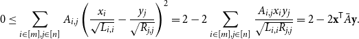 \begin{equation*}0\leq \sum _{i\in [m], j \in [n]}A_{i,j}\left (\frac {x_i}{\sqrt {L_{i,i}}}-\frac {y_j}{\sqrt {R_{j,j}}}\right )^2=2-2\sum _{i\in [m], j \in [n]}\frac {A_{i,j}x_iy_j}{\sqrt {L_{i,i}R_{j,j}}}=2-2\mathbf {x}^{\mathsf {T}} \bar {A} \mathbf {y}.\end{equation*}
This implies that $\mathbf {x}^{\mathsf {T}} \bar {A} \mathbf {y}\leq 1$
for all unit vectors
$\mathbf {x}^{\mathsf {T}} \bar {A} \mathbf {y}\leq 1$
for all unit vectors $\mathbf {x}$
and
$\mathbf {x}$
and $\mathbf {y}$
, which yields
$\mathbf {y}$
, which yields $\|\bar {A}\|\leq 1$
.
$\|\bar {A}\|\leq 1$
.
Moreover, by definition of $\bar {A}$
, we have
$\bar {A}$
, we have $\mathbf {u}_1^{\mathsf {T}} \bar {A} {\mathbf {v}}_1=1$
. Therefore, by definition of the operator norm, it follows that
$\mathbf {u}_1^{\mathsf {T}} \bar {A} {\mathbf {v}}_1=1$
. Therefore, by definition of the operator norm, it follows that $\|{\bar {A}}\| \ge 1$
. The observation is proved.
$\|{\bar {A}}\| \ge 1$
. The observation is proved.
Now we are ready to prove Theorem3.4.
Proof of Theorem 3.4. Let $r={rank}(\bar {A})$
, and let
$r={rank}(\bar {A})$
, and let $1=s_1 \geq s_2 \geq \ldots \geq s_r\gt 0$
be all the positive singular values of
$1=s_1 \geq s_2 \geq \ldots \geq s_r\gt 0$
be all the positive singular values of $\bar {A}$
in nonincreasing order. Applying the singular value decomposition theorem (TheoremA.3) combined with Observation 3.5, we can find orthonormal bases
$\bar {A}$
in nonincreasing order. Applying the singular value decomposition theorem (TheoremA.3) combined with Observation 3.5, we can find orthonormal bases $\{\mathbf {u}_1,\ldots, \mathbf {u}_m\}$
of
$\{\mathbf {u}_1,\ldots, \mathbf {u}_m\}$
of $\mathbb {R}^m$
and
$\mathbb {R}^m$
and $\{{\mathbf {v}}_1,\ldots, {\mathbf {v}}_n\}$
of
$\{{\mathbf {v}}_1,\ldots, {\mathbf {v}}_n\}$
of $\mathbb {R}^n$
with vectors
$\mathbb {R}^n$
with vectors ${\mathbf {v}}_1$
and
${\mathbf {v}}_1$
and $\mathbf {u}_1$
defined in Observation 3.5, and such that
$\mathbf {u}_1$
defined in Observation 3.5, and such that
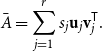 \begin{equation*} \bar {A}=\sum _{j=1}^r s_j \mathbf {u}_j {\mathbf {v}}_j^{\mathsf {T}}. \end{equation*}
In particular, $\bar {A}{\mathbf {v}}_j=s_j\mathbf {u}_j$
for
$\bar {A}{\mathbf {v}}_j=s_j\mathbf {u}_j$
for $j=1,\ldots, r$
and
$j=1,\ldots, r$
and $\bar {A}{\mathbf {v}}_j=\mathbf {0}$
for
$\bar {A}{\mathbf {v}}_j=\mathbf {0}$
for $j\gt r$
. Now, let
$j\gt r$
. Now, let $S\subseteq [m]$
and
$S\subseteq [m]$
and $T\subseteq [n]$
be two arbitrary subsets. Then
$T\subseteq [n]$
be two arbitrary subsets. Then
 \begin{equation*} A(S,T) = \unicode {x1D7D9}_S^{\mathsf {T}} A \unicode {x1D7D9}_T = \chi _S^{\mathsf {T}} \bar {A} \chi _T, \quad \text {where} \quad \chi _S \,:\!=\, L^{1/2}\unicode {x1D7D9}_S, \quad \chi _T \,:\!=\, R^{1/2}\unicode {x1D7D9}_T. \end{equation*}
Expanding both vectors as
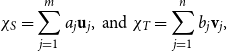 \begin{equation*}\chi _S=\sum _{j=1}^m a_j\mathbf {u}_j, \textrm { and } \chi _T=\sum _{j=1}^n b_j{\mathbf {v}}_j,\end{equation*}
we obtain
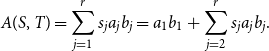 \begin{equation*} A(S,T) = \sum _{j=1}^r s_j a_j b_j = a_1 b_1 + \sum _{j=2}^r s_j a_j b_j. \end{equation*}
Recall from Observation 3.5 that all singular values of $\bar {A}$
are bounded by
$\bar {A}$
are bounded by $1$
, and
$1$
, and $r = {rank}(\bar {A}) \le \min \{m,n\}$
. Thus, by Cauchy–Schwarz inequality, we have
$r = {rank}(\bar {A}) \le \min \{m,n\}$
. Thus, by Cauchy–Schwarz inequality, we have
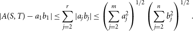 \begin{equation} |A(S,T) - a_1 b_1 | \le \sum _{j=2}^r|a_j b_j| \le \left ( \sum _{j=2}^m a_j^2 \right )^{1/2} \left ( \sum _{j=2}^n b_j^2 \right )^{1/2}. \end{equation}
Now observe that $a_1=\left \langle \chi _S,\mathbf {u}_1\right \rangle = a^{-1/2} A(S,n)$
and
$a_1=\left \langle \chi _S,\mathbf {u}_1\right \rangle = a^{-1/2} A(S,n)$
and $b_1=\left \langle \chi _T,{\mathbf {v}}_1\right \rangle = a^{-1/2} A(m,T)$
, so
$b_1=\left \langle \chi _T,{\mathbf {v}}_1\right \rangle = a^{-1/2} A(m,T)$
, so
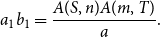 \begin{equation*} a_1 b_1 = \frac {A(S,n) A(m,T)}{a}. \end{equation*}
Moreover,
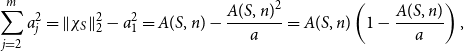 \begin{equation*} \sum _{j=2}^m a_j^2 = \|{\chi _S}\|_2^2 - a_1^2 = A(S,n) - \frac {A(S,n)^2}{a} = A(S,n)\left (1-\frac {A(S,n)}{a}\right ), \end{equation*}
and similarly
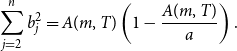 \begin{equation*} \sum _{j=2}^n b_j^2 = A(m,T) \left (1-\frac {A(m,T)}{a}\right ). \end{equation*}
Substitute the last three identities into (1) to complete the proof.
4. Almost regular expanders
Our argument relies on some spectral properties of random subgraphs of $(n,d,\lambda )$
-graphs. Since random subgraphs are not expected to be exactly regular, we extend the definition of
$(n,d,\lambda )$
-graphs. Since random subgraphs are not expected to be exactly regular, we extend the definition of $(n,d,\lambda )$
-graphs as follows:
$(n,d,\lambda )$
-graphs as follows:
Definition 4.1 (Almost $(n,d,\lambda )$
-graphs). Let
$(n,d,\lambda )$
-graphs). Let $d,\lambda \gt 0$
and
$d,\lambda \gt 0$
and $\gamma \in [0,1)$
. We say that a graph
$\gamma \in [0,1)$
. We say that a graph $G$
is an
$G$
is an $(n, (1\pm \gamma )d, \lambda )$
-graph if
Footnote
1
$(n, (1\pm \gamma )d, \lambda )$
-graph if
Footnote
1 $G$
is a graph on
$G$
is a graph on $n$
vertices whose all degrees are
$n$
vertices whose all degrees are $(1\pm \gamma )d$
and the second singular value of the adjacency matrix
$(1\pm \gamma )d$
and the second singular value of the adjacency matrix $A$
of
$A$
of $G$
satisfies
$G$
satisfies $s_2(A) \le \lambda$
.
$s_2(A) \le \lambda$
.
Almost $(n,d,\lambda )$
-graphs behave similar to exact
$(n,d,\lambda )$
-graphs behave similar to exact $(n,d,\lambda )$
-graphs in many ways. If
$(n,d,\lambda )$
-graphs in many ways. If $G$
is an (exactly)
$G$
is an (exactly) $d$
-regular graph with adjacency matrix
$d$
-regular graph with adjacency matrix $A$
, its normalized adjacency matrix is obviously
$A$
, its normalized adjacency matrix is obviously
 \begin{equation*} \bar {A}=\frac {1}{d}A \end{equation*}
according to Definition 3.2. If $G$
is an almost
$G$
is an almost $d$
-regular graph, its degree matrix
$d$
-regular graph, its degree matrix $D=diag(d_1,\ldots, d_n)$
is close to
$D=diag(d_1,\ldots, d_n)$
is close to $dI$
, and we can expect that
$dI$
, and we can expect that
 \begin{equation*} \bar {A} = D^{-1/2} A D^{-1/2} \approx \frac {1}{d}A \end{equation*}
in some sense. Below we show that such an approximation indeed holds in the sense of the closeness of all singular values.
Corollary 4.2 (Singular values of almost regular graphs). Let $\gamma \in [0,1)$
and
$\gamma \in [0,1)$
and $d\gt 0$
. Let
$d\gt 0$
. Let $G$
be a graph whose all vertices have degrees
$G$
be a graph whose all vertices have degrees $(1\pm \gamma )d$
. Then the adjacency matrix
$(1\pm \gamma )d$
. Then the adjacency matrix $A$
and the normalized adjacency matrix
$A$
and the normalized adjacency matrix $\bar {A}$
of the graph
$\bar {A}$
of the graph $G$
satisfy
$G$
satisfy
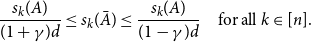 \begin{equation*} \frac {s_k(A)}{(1+\gamma )d} \le s_k(\bar {A}) \le \frac {s_k(A)}{(1-\gamma )d} \quad \text {for all } k \in [n]. \end{equation*}
Proof. Using the chain rule for singular values (Lemma A.5), we obtain
 \begin{equation*} s_k(A) = s_k \left ( D^{1/2}\bar {A}D^{1/2} \right ) \le \|{D^{1/2}}\|^2 s_k(\bar {A}). \end{equation*}
Since $\|{D^{1/2}}\|^2 = \|{D}\| = \max _i d_i \le (1+\gamma )d$
, the lower bound in Corollary 4.2 follows. The upper bound can be proved similarly.
$\|{D^{1/2}}\|^2 = \|{D}\| = \max _i d_i \le (1+\gamma )d$
, the lower bound in Corollary 4.2 follows. The upper bound can be proved similarly.
4.1 Expander mixing lemma for almost regular expanders
Let us specialize Theorem3.4 for almost $(n,d,\lambda )$
-graphs.
$(n,d,\lambda )$
-graphs.
Corollary 4.3 (Expander mixing lemma for almost $(n,d,\lambda )$
-graphs). Let
$(n,d,\lambda )$
-graphs). Let $G$
be an
$G$
be an $(n,(1\pm \gamma )d,\lambda )$
-graph. Then, for any two subsets
$(n,(1\pm \gamma )d,\lambda )$
-graph. Then, for any two subsets $S,T\subseteq V(G)$
, we have
$S,T\subseteq V(G)$
, we have
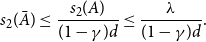
 \begin{equation} \frac {(1-\gamma )^2d|S||T|}{(1+\gamma )n}-{\varepsilon } \leq e(S,T) \leq \frac {(1+\gamma )^2d|S||T|}{(1-\gamma )n}+{\varepsilon }, \end{equation}
where
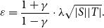 \begin{equation*} {\varepsilon }=\frac {1+\gamma }{1-\gamma }\cdot \lambda \sqrt {|S||T|}. \end{equation*}
Proof.
Let $A$
and
$A$
and $\bar {A}$
be the adjacency and the normalized adjacency matrices of
$\bar {A}$
be the adjacency and the normalized adjacency matrices of $G$
, respectively. Theorem3.4 yields
$G$
, respectively. Theorem3.4 yields
 \begin{equation} \left |A(S,T)-\frac {A(S,n) \, A(n,T)}{A(n,n)}\right | \leq s_2(\bar {A})\sqrt {A(S,n) A(n,T)}. \end{equation}
By Corollary 4.2 and assumption, we have
 \begin{equation*} s_2(\bar {A}) \le \frac {s_2(A)}{(1-\gamma )d} \le \frac {\lambda }{(1-\gamma )d}. \end{equation*}
Moreover, since $A$
is an adjacency matrix, we have
$A$
is an adjacency matrix, we have $A(S,T)=e(S,T)$
,
$A(S,T)=e(S,T)$
, $A(S,n) = \sum _{v\in S}\deg (v) = (1\pm \gamma )d |S|$
,
$A(S,n) = \sum _{v\in S}\deg (v) = (1\pm \gamma )d |S|$
, $A(n,T) = \sum _{v\in T}\deg (v) = (1\pm \gamma )d |T|$
,
$A(n,T) = \sum _{v\in T}\deg (v) = (1\pm \gamma )d |T|$
, $A(n,n) = \sum _{v\in V(G)}\deg (v) = (1\pm \gamma )d |V(G)| = (1\pm \gamma )dn$
. Substitute all this into (3) and use triangle inequality to complete the proof.
$A(n,n) = \sum _{v\in V(G)}\deg (v) = (1\pm \gamma )d |V(G)| = (1\pm \gamma )dn$
. Substitute all this into (3) and use triangle inequality to complete the proof.
Sometimes all we need is at least one edge between disjoint sets of vertices $S$
and
$S$
and $T$
. Corollary 4.3 provides a convenient sufficient condition for this:
$T$
. Corollary 4.3 provides a convenient sufficient condition for this:
Corollary 4.4 (At least one edge). Let $G$
be an
$G$
be an $(n,(1\pm \gamma )d,\lambda )$
-graph. Let
$(n,(1\pm \gamma )d,\lambda )$
-graph. Let $S,T\subseteq V(G)$
be two disjoint subsets with
$S,T\subseteq V(G)$
be two disjoint subsets with
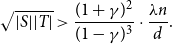 \begin{equation*} \sqrt {|S||T|} \gt \frac {(1+\gamma )^2}{(1-\gamma )^3} \cdot \frac {\lambda n}{d}. \end{equation*}
Then $e(S,T)\gt 0$
.
$e(S,T)\gt 0$
.
Proof. Under our assumptions, the lower bound in (2) is strictly positive.
The following statement, which is another simple corollary of the expander mixing lemma, allows us to translate minimum degree conditions into an expansion property for small sets.
Lemma 4.5.
Let $\gamma \in [0,1/20]$
be a constant, and let
$\gamma \in [0,1/20]$
be a constant, and let $\lambda \leq d/700$
. Let
$\lambda \leq d/700$
. Let $G$
be an
$G$
be an $(n,(1\pm \gamma )d,\lambda )$
-graph which contains subsets
$(n,(1\pm \gamma )d,\lambda )$
-graph which contains subsets $S,T\subset V(G)$
such that for every
$S,T\subset V(G)$
such that for every $v\in S$
,
$v\in S$
, $d(v,T)\geq d/6$
. Then, every subset
$d(v,T)\geq d/6$
. Then, every subset $X\subset S$
of size
$X\subset S$
of size $|X|\le \frac {4\lambda n}{d}$
satisfies
$|X|\le \frac {4\lambda n}{d}$
satisfies $|N(X, T)|\geq \frac {d}{700\lambda }|X|$
.
$|N(X, T)|\geq \frac {d}{700\lambda }|X|$
.
Proof.
Let $D=\frac {d}{700\lambda }\geq 1$
. Suppose that there exists a subset
$D=\frac {d}{700\lambda }\geq 1$
. Suppose that there exists a subset $X\subset S$
of size
$X\subset S$
of size $1\le |X|\le \frac {4\lambda n}{d}$
such that
$1\le |X|\le \frac {4\lambda n}{d}$
such that $|N(X,T)|\lt D|X|$
. Let
$|N(X,T)|\lt D|X|$
. Let $Y=N(X,T)$
. Corollary 4.3 implies that
$Y=N(X,T)$
. Corollary 4.3 implies that
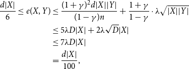 \begin{equation*} \begin{aligned} \frac {d|X|}{6}\leq e(X,Y) &\leq \frac {(1+\gamma )^2d|X||Y|}{(1-\gamma )n}+\frac {1+\gamma }{1-\gamma }\cdot \lambda \sqrt {|X||Y|}\\ &\le 5\lambda D|X|+2\lambda \sqrt {D}|X|\\ &\leq 7\lambda D|X|\\ &=\frac {d|X|}{100}, \end{aligned}\end{equation*}
which is a contradiction. Therefore, every subset $X\subset S$
of size
$X\subset S$
of size $|X|\le \frac {4\lambda n}{d}$
satisfies
$|X|\le \frac {4\lambda n}{d}$
satisfies $|N(X,T)|\geq \frac {d}{700\lambda }|X|$
. The proof is completed.
$|N(X,T)|\geq \frac {d}{700\lambda }|X|$
. The proof is completed.
4.2 Matchings in almost regular expanders
In this section, we use the expander mixing lemma to get some corollaries for matchings in almost $(n,d,\lambda )$
-graphs. For our convenience, we define the bipartite spectral expanders as below.
$(n,d,\lambda )$
-graphs. For our convenience, we define the bipartite spectral expanders as below.
Definition 4.6.
We say that a bipartite graph $H = (V_1 \cup V_2, E)$
is an
$H = (V_1 \cup V_2, E)$
is an $(n, (1 \pm \gamma )d, \lambda )$
-bipartite expander if
$(n, (1 \pm \gamma )d, \lambda )$
-bipartite expander if $H$
is an induced bipartite subgraph of an
$H$
is an induced bipartite subgraph of an $(n, (1 \pm \gamma )d, \lambda )$
-graph
$(n, (1 \pm \gamma )d, \lambda )$
-graph $G$
with
$G$
with $V(G) = V_1 \cup V_2$
, and for each
$V(G) = V_1 \cup V_2$
, and for each $i = 1, 2$
and every
$i = 1, 2$
and every $v \in V_i$
, the degree of
$v \in V_i$
, the degree of $v$
in
$v$
in $H$
satisfies
$H$
satisfies $\deg _H(v) = (1 \pm \gamma ) \frac {d |V_{3-i}|}{n}$
.
$\deg _H(v) = (1 \pm \gamma ) \frac {d |V_{3-i}|}{n}$
.
First, we prove the existence of perfect matchings in a bipartite spectral expander with a balanced bipartition.
Lemma 4.7.
Let $\gamma \in [0,1/6]$
be a constant, let
$\gamma \in [0,1/6]$
be a constant, let $d\gt 0$
and let
$d\gt 0$
and let $\lambda \leq d/200$
. Let
$\lambda \leq d/200$
. Let $G=(V,E)$
be an
$G=(V,E)$
be an $(n,(1\pm \gamma )d,\lambda )$
-bipartite expander with parts
$(n,(1\pm \gamma )d,\lambda )$
-bipartite expander with parts $V=V_1\cup V_2$
such that
$V=V_1\cup V_2$
such that $|V_1|=|V_2|$
. Then
$|V_1|=|V_2|$
. Then $G$
contains a perfect matching.
$G$
contains a perfect matching.
Proof.
It is enough to verify the following condition which is equivalent to Hall’s condition (see Theorem 3.1.11 in [Reference West42]): for all $i\in [2]$
and
$i\in [2]$
and $S\subseteq V_i$
of size
$S\subseteq V_i$
of size $|S|\leq |V_i|/2$
, we have
$|S|\leq |V_i|/2$
, we have $|N(S)|\geq |S|$
.
$|N(S)|\geq |S|$
.
Suppose to the contrary that there exists $i\in [2]$
and an
$i\in [2]$
and an $S\subseteq V_i$
, such that the set
$S\subseteq V_i$
, such that the set $T\,:\!=\, N(S)$
is of size less than
$T\,:\!=\, N(S)$
is of size less than $|S|$
. Since
$|S|$
. Since $G$
is an
$G$
is an $(n,(1\pm \gamma )d,\lambda )$
-bipartite expander and since
$(n,(1\pm \gamma )d,\lambda )$
-bipartite expander and since $|V_1|=|V_2|=n/2$
, we have that
$|V_1|=|V_2|=n/2$
, we have that
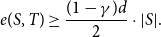 \begin{equation*} e(S,T)\geq \frac {(1-\gamma )d}{2}\cdot |S|. \end{equation*}
On the other hand, using the assumption that $\gamma \leq 1/6$
and the expander mixing lemma for almost regular expanders (Corollary 4.3), we obtain that
$\gamma \leq 1/6$
and the expander mixing lemma for almost regular expanders (Corollary 4.3), we obtain that
 \begin{equation*} e(S,T)\leq \frac {(1+\gamma )^2d|S||T|}{(1-\gamma )n}+\frac {1+\gamma }{1-\gamma }\cdot \lambda \sqrt {|S||T|}\leq \frac {49d|S|}{120}+\frac {7d|S|}{1000}\lt \frac {(1-\gamma )d}{2}\cdot |S|, \end{equation*}
where we also used $|T|\lt |S|\le n/4$
and
$|T|\lt |S|\le n/4$
and $\lambda \le d/200$
.
$\lambda \le d/200$
.
Combining these two estimates we obtain a contradiction. This completes the proof.
If finding a perfect matching is not necessary, then following from Corollary 4.4, we can use a greedy algorithm to find a matching that avoids a not-too-large subset in each part of a bipartite expander.
Lemma 4.8.
Let $G$
be an
$G$
be an $(n,(1\pm \gamma )d,\lambda )$
-graph, and let
$(n,(1\pm \gamma )d,\lambda )$
-graph, and let $V(G)=V_1\cup V_2$
be a partition. For each
$V(G)=V_1\cup V_2$
be a partition. For each $i=1,2$
, let
$i=1,2$
, let $S_i\subseteq V_i$
be a subset of size
$S_i\subseteq V_i$
be a subset of size $0\leq k_i\leq |V_i|-\frac {(1+\gamma )^2}{(1-\gamma )^3} \cdot \frac {\lambda n}{d}$
. Then there exists a matching of size
$0\leq k_i\leq |V_i|-\frac {(1+\gamma )^2}{(1-\gamma )^3} \cdot \frac {\lambda n}{d}$
. Then there exists a matching of size
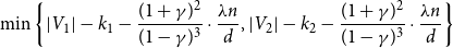 \begin{equation*} \min \left \{|V_1|-k_1-\frac {(1+\gamma )^2}{(1-\gamma )^3} \cdot \frac {\lambda n}{d},|V_2|-k_2-\frac {(1+\gamma )^2}{(1-\gamma )^3} \cdot \frac {\lambda n}{d}\right \} \end{equation*}
in $G$
between
$G$
between $V_1\setminus S_1$
and
$V_1\setminus S_1$
and $V_2\setminus S_2$
.
$V_2\setminus S_2$
.
Proof.
We find the matching between $V_1\setminus S_1$
and
$V_1\setminus S_1$
and $V_2\setminus S_2$
greedily. Initially, let
$V_2\setminus S_2$
greedily. Initially, let $M\,:\!=\, \emptyset$
, and let
$M\,:\!=\, \emptyset$
, and let $U_1\,:\!=\, V_1\setminus S_1$
and
$U_1\,:\!=\, V_1\setminus S_1$
and $U_2\,:\!=\, V_2\setminus S_2$
. If
$U_2\,:\!=\, V_2\setminus S_2$
. If $|U_1|\leq \frac {(1+\gamma )^2}{(1-\gamma )^3} \cdot \frac {\lambda n}{d}$
or
$|U_1|\leq \frac {(1+\gamma )^2}{(1-\gamma )^3} \cdot \frac {\lambda n}{d}$
or $|U_2|\leq \frac {(1+\gamma )^2}{(1-\gamma )^3} \cdot \frac {\lambda n}{d}$
, then we stop. Otherwise, by Corollary 4.4, there is an edge
$|U_2|\leq \frac {(1+\gamma )^2}{(1-\gamma )^3} \cdot \frac {\lambda n}{d}$
, then we stop. Otherwise, by Corollary 4.4, there is an edge $e\in E(G)$
between
$e\in E(G)$
between $U_1$
and
$U_1$
and $U_2$
. Let
$U_2$
. Let $M\,:\!=\, M\cup \{e\}$
, and let
$M\,:\!=\, M\cup \{e\}$
, and let $U_1\,:\!=\, U_1\setminus V(e)$
and
$U_1\,:\!=\, U_1\setminus V(e)$
and $U_2\,:\!=\, U_2\setminus V(e)$
. Continuing in this fashion, we obtain a matching
$U_2\,:\!=\, U_2\setminus V(e)$
. Continuing in this fashion, we obtain a matching $M$
of size
$M$
of size $\min \left \{|V_1|-k_1-\frac {(1+\gamma )^2}{(1-\gamma )^3} \cdot \frac {\lambda n}{d},|V_2|-k_2-\frac {(1+\gamma )^2}{(1-\gamma )^3} \cdot \frac {\lambda n}{d}\right \}$
in
$\min \left \{|V_1|-k_1-\frac {(1+\gamma )^2}{(1-\gamma )^3} \cdot \frac {\lambda n}{d},|V_2|-k_2-\frac {(1+\gamma )^2}{(1-\gamma )^3} \cdot \frac {\lambda n}{d}\right \}$
in $G$
between
$G$
between $V_1\setminus S_1$
and
$V_1\setminus S_1$
and $V_2\setminus S_2$
. The proof is completed.
$V_2\setminus S_2$
. The proof is completed.
5. Extendability
In [Reference Hyde, Morrison, Müyesser and Pavez-Signé20], the classical tree embedding technique, introduced by Friedman and Pippenger in [Reference Friedman and Pippenger11], was used as one of the tools to prove a useful result on connecting designated pairs of vertices in expander graphs. The result shows that given two “nice” disjoint small subsets of an $(n,d,\lambda )$
-graph, one can find a small subgraph, disjoint from these subsets, such that for any designated ordering of vertex pairs from the subsets, there exists a path factor in the subgraph that connects the pairs.
$(n,d,\lambda )$
-graph, one can find a small subgraph, disjoint from these subsets, such that for any designated ordering of vertex pairs from the subsets, there exists a path factor in the subgraph that connects the pairs.
Definition 5.1.
Let $D,m\in \mathbb N$
with
$D,m\in \mathbb N$
with $D\ge 3$
. Let
$D\ge 3$
. Let $G$
be a graph and let
$G$
be a graph and let $S\subset G$
be a subgraph with
$S\subset G$
be a subgraph with $\Delta (S) \leq D$
. We say that
$\Delta (S) \leq D$
. We say that $S$
is
$S$
is $(D,m)$
-extendable if for all
$(D,m)$
-extendable if for all $U\subset V(G)$
with
$U\subset V(G)$
with $1\le |U|\le 2m$
we have
$1\le |U|\le 2m$
we have
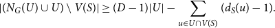 \begin{equation*} |(N_G(U)\cup U)\setminus V(S)|\ge (D-1)|U|-\sum _{u\in U\cap V(S)}(d_S(u)-1). \end{equation*}
The following result says that it is enough to control the external neighbourhood of small sets in order to verify extendability.
Proposition 5.2.
[Reference Hyde, Morrison, Müyesser and Pavez-Signé20] Let $D,m\in \mathbb N$
with
$D,m\in \mathbb N$
with $D\ge 3$
. Let
$D\ge 3$
. Let $G$
be a graph and let
$G$
be a graph and let $S\subset G$
be a subgraph with
$S\subset G$
be a subgraph with $\Delta (S)\le D$
. If for all
$\Delta (S)\le D$
. If for all $U\subset V(G)$
with
$U\subset V(G)$
with $1\leq |U|\leq 2m$
we have
$1\leq |U|\leq 2m$
we have
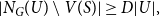 \begin{equation*}|N_G(U)\setminus V(S)|\geq D|U|,\end{equation*}
then $S$
is
$S$
is $(D,m)$
-extendable in
$(D,m)$
-extendable in $G$
.
$G$
.
Before stating the lemma, we introduce some necessary definitions. We denote by $I(S)$
the edgeless subgraph with vertex set
$I(S)$
the edgeless subgraph with vertex set $S$
. A graph
$S$
. A graph $G$
is said to be
$G$
is said to be $m$
-joined if for any disjoint sets
$m$
-joined if for any disjoint sets $A, B \subseteq V(G)$
with
$A, B \subseteq V(G)$
with $|A|, |B| \geq m$
, there is at least one edge between
$|A|, |B| \geq m$
, there is at least one edge between $A$
and
$A$
and $B$
, i.e.,
$B$
, i.e., $e(A, B) \geq 1$
.
$e(A, B) \geq 1$
.
Now we are ready to state the result from [Reference Hyde, Morrison, Müyesser and Pavez-Signé20].
Lemma 5.3.
There is an absolute constant $C\gt 0$
with the following property. Let
$C\gt 0$
with the following property. Let $n$
be a sufficiently large integer, and let
$n$
be a sufficiently large integer, and let $20C\leq K\leq n/\log ^3n$
. Let
$20C\leq K\leq n/\log ^3n$
. Let $D,m\in \mathbb {N}$
satisfy
$D,m\in \mathbb {N}$
satisfy $m\leq n/100D$
and
$m\leq n/100D$
and $D\ge 100$
. Let
$D\ge 100$
. Let $G$
be an
$G$
be an $m$
-joined graph on
$m$
-joined graph on $n$
vertices which contains disjoint subsets
$n$
vertices which contains disjoint subsets $V_1, V_2\subseteq V(G)$
with
$V_1, V_2\subseteq V(G)$
with $|V_1|=|V_2|\leq n/K\log ^{3}n$
, and set
$|V_1|=|V_2|\leq n/K\log ^{3}n$
, and set $\ell \,:\!=\,\lfloor C \log ^3 n \rfloor$
. Suppose that
$\ell \,:\!=\,\lfloor C \log ^3 n \rfloor$
. Suppose that $I(V_1\cup V_2)$
is
$I(V_1\cup V_2)$
is $(D,m)$
-extendable in
$(D,m)$
-extendable in $G$
.
$G$
.
Then, there exists a $(D,m)$
-extendable subgraph
$(D,m)$
-extendable subgraph $S_{res}\subseteq G$
such that for any bijection
$S_{res}\subseteq G$
such that for any bijection $\phi \colon V_1\to V_2$
, there exists a
$\phi \colon V_1\to V_2$
, there exists a $P_\ell$
-factor of
$P_\ell$
-factor of $S_{res}$
where each copy of
$S_{res}$
where each copy of $P_\ell$
has as its endpoints some
$P_\ell$
has as its endpoints some $v\in V_1$
and
$v\in V_1$
and $\phi (v)\in V_2$
.
$\phi (v)\in V_2$
.
6. Random subgraphs of almost regular expanders
In this section, we show that a random induced subgraph of an almost $(n,d,\lambda )$
-graph or a bipartite spectral expander is typically a spectral expander by itself. This serves as our main tool in the proof of our main result.
$(n,d,\lambda )$
-graph or a bipartite spectral expander is typically a spectral expander by itself. This serves as our main tool in the proof of our main result.
6.1 Chernoff’s bounds
We extensively use the following well-known Chernoff’s bounds for the upper and lower tails of the hypergeometric distribution throughout the paper. The following lemma was proved by Hoeffding [Reference Hoeffding18] (also see Section 23.5 in [Reference Frieze and Karoński13]).
Lemma 6.1 (Chernoff’s inequality for hypergeometric distribution). Let $X\sim \mathrm {Hypergeometric} (N,K,n)$
and let
$X\sim \mathrm {Hypergeometric} (N,K,n)$
and let $\mathbb {E}[X]=\mu$
. Then
$\mathbb {E}[X]=\mu$
. Then
-
•
$\mathbb {P} \left [ X\lt (1-a)\mu \right ]\lt e^{-a^2\mu /2}$
for every
$a\gt 0$
; -
•
$\mathbb {P} \left [ X\gt (1+a)\mu \right ]\lt e^{-a^2\mu /3}$
for every
$a\in (0,\frac {3}{2})$
.


6.2 Random-induced subgraphs
The following theorem is the main result of this section. It asserts that with probability at least $1-n^{-\Theta (1)}$
, random (induced) subgraphs of spectral expanders are also spectral expanders.
$1-n^{-\Theta (1)}$
, random (induced) subgraphs of spectral expanders are also spectral expanders.
Theorem 6.2 (Random subgraphs of spectral expanders). Let $\gamma \in (0,1/200]$
be a constant. There exists an absolute constant
$\gamma \in (0,1/200]$
be a constant. There exists an absolute constant $C$
such that the following holds for sufficiently large
$C$
such that the following holds for sufficiently large $n$
. Let
$n$
. Let $d,\lambda \gt 0$
, let
$d,\lambda \gt 0$
, let $\sigma \in [1/n,1)$
, and let
$\sigma \in [1/n,1)$
, and let $G$
be an
$G$
be an $(n,(1\pm \gamma )d,\lambda )$
-graph. Let
$(n,(1\pm \gamma )d,\lambda )$
-graph. Let $X\subseteq V(G)$
with
$X\subseteq V(G)$
with $|X|=\sigma n$
be a subset chosen uniformly at random, and let
$|X|=\sigma n$
be a subset chosen uniformly at random, and let $H \,:\!=\, G[X]$
be the subgraph of
$H \,:\!=\, G[X]$
be the subgraph of $G$
induced by
$G$
induced by $X$
. Assume that
$X$
. Assume that
 \begin{equation*} \sigma d\ge C \gamma ^{-2} \log n \quad \text {and} \quad \sigma \lambda \ge C\sqrt {\sigma d\log n}. \end{equation*}
Then with probability at least $1-n^{-1/6}$
,
$1-n^{-1/6}$
, $H$
is a
$H$
is a $\left (\sigma n, (1\pm 2\gamma )\sigma d, 6\sigma \lambda \right )$
-graph.
$\left (\sigma n, (1\pm 2\gamma )\sigma d, 6\sigma \lambda \right )$
-graph.
Let us briefly discuss the two conditions in Theorem6.2. The first condition permits the random subgraph to be quite sparse – with degrees on the order of $\log n$
– but not sparser than that. Below this threshold, the degrees of the random subgraph become unstable, and it will no longer be approximately regular. The second condition is essentially the Alon-Boppana bound, up to a logarithmic factor, which dictates that the second singular value of an approximately
$\log n$
– but not sparser than that. Below this threshold, the degrees of the random subgraph become unstable, and it will no longer be approximately regular. The second condition is essentially the Alon-Boppana bound, up to a logarithmic factor, which dictates that the second singular value of an approximately $\sigma d$
-regular graph must be at least
$\sigma d$
-regular graph must be at least $\Omega (\sqrt {\sigma d})$
. In other words, the conditions in Theorem6.2 are nearly necessary for a subgraph
$\Omega (\sqrt {\sigma d})$
. In other words, the conditions in Theorem6.2 are nearly necessary for a subgraph $H$
to be an almost regular expander. Additionally, we did not optimise the constant factor in
$H$
to be an almost regular expander. Additionally, we did not optimise the constant factor in $s_2(H)$
, though we believe it should be
$s_2(H)$
, though we believe it should be $1 + o(1)$
.
$1 + o(1)$
.
The proof of Theorem6.2 is based on bounds of the spectral norm of a random submatrix, which is obtained from a given $n \times n$
matrix
$n \times n$
matrix $B$
by choosing a uniformly random subset of rows and a uniformly random subset of columns of
$B$
by choosing a uniformly random subset of rows and a uniformly random subset of columns of $B$
.
$B$
.
There are two natural ways to choose a random subset of the set $[n]$
. We can make a random subset
$[n]$
. We can make a random subset $I$
by selecting every element of
$I$
by selecting every element of $[n]$
independently at random with probability
$[n]$
independently at random with probability $\sigma \in (0,1)$
. In this case, we write
$\sigma \in (0,1)$
. In this case, we write
 \begin{equation*} I \sim \mathrm{Subset} (n,\sigma ). \end{equation*}
Alternatively, we can choose any $m$
-set
$m$
-set $J$
of
$J$
of $[n]$
with the same probability
$[n]$
with the same probability $1/\binom {n}{m}$
. In this case, we write
$1/\binom {n}{m}$
. In this case, we write
 \begin{equation*} J \sim \mathrm{Subset} (n,m). \end{equation*}
Note that if $m = \sigma n$
, the models
$m = \sigma n$
, the models $\textrm {Subset}(n,\sigma )$
and
$\textrm {Subset}(n,\sigma )$
and $\textrm {Subset}(n,m)$
are closely related but not identical. It should be clear from the context which one we consider.
$\textrm {Subset}(n,m)$
are closely related but not identical. It should be clear from the context which one we consider.
For a given subset $I \subset [n]$
, we denote by
$I \subset [n]$
, we denote by $P_I$
the orthogonal projection in
$P_I$
the orthogonal projection in ${\mathbb {R}}^n$
onto
${\mathbb {R}}^n$
onto ${\mathbb {R}}^I$
. In other words,
${\mathbb {R}}^I$
. In other words, $P_I$
is the diagonal matrix with
$P_I$
is the diagonal matrix with $P_{ii}=1$
if
$P_{ii}=1$
if $i \in I$
and
$i \in I$
and $P_{ii}=0$
if
$P_{ii}=0$
if $i \not \in I$
.
$i \not \in I$
.
The main tool of this section is the following bound. It is worth mentioning that several similar results have been proved before, for example, in [Reference Rudelson and Vershynin35] and [Reference Tropp41].
Theorem 6.3 (Norms of random submatrices). Let $B$
be an
$B$
be an $n\times n$
matrix. Let
$n\times n$
matrix. Let $I,I' \sim \textrm {Subset}(n,\sigma )$
be two independent subsets, where
$I,I' \sim \textrm {Subset}(n,\sigma )$
be two independent subsets, where $\sigma \in (0,1)$
. Let
$\sigma \in (0,1)$
. Let $p\geq 2$
and let
$p\geq 2$
and let $q=\max \{p,2\log n\}$
. Then
$q=\max \{p,2\log n\}$
. Then
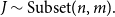
 \begin{equation*} \mathbb {E}_p\|{P_I B P_{I'}}\| \le \sigma \|{B}\| + 3\sqrt {q\sigma }\left ( \|{B}\|_{1\rightarrow 2} + \|{B^{\mathsf {T}}}\|_{1\rightarrow 2} \right ) + 8q\|{B}\|_\infty . \end{equation*}
Here $\mathbb {E}_p[X]=(\mathbb {E}|X|^p)^{1/p}$
is the
$\mathbb {E}_p[X]=(\mathbb {E}|X|^p)^{1/p}$
is the $L_p$
norm of the random variable
$L_p$
norm of the random variable $X$
; the norm
$X$
; the norm $\|{\mkern 2mu\cdot \mkern 2mu}\|_{1\to 2}$
denotes the norm of a matrix as an
$\|{\mkern 2mu\cdot \mkern 2mu}\|_{1\to 2}$
denotes the norm of a matrix as an $\ell _1 \to \ell _2$
linear operator, which equals to the maximum value among the
$\ell _1 \to \ell _2$
linear operator, which equals to the maximum value among the $\ell _2$
norm of each column; and
$\ell _2$
norm of each column; and $\|{\cdot }\|_\infty$
denotes the maximum absolute entry of a matrix.
$\|{\cdot }\|_\infty$
denotes the maximum absolute entry of a matrix.
We use the following results to derive Theorem6.3.
Lemma 6.4 (Rudelson-Vershynin [Reference Rudelson and Vershynin35]). Let $A$
be an
$A$
be an $m\times n$
matrix with rank
$m\times n$
matrix with rank $r$
. Let
$r$
. Let $I \sim \textrm {Subset}(n,\sigma )$
, where
$I \sim \textrm {Subset}(n,\sigma )$
, where $\sigma \in (0,1)$
. Let
$\sigma \in (0,1)$
. Let $p \ge 2$
and let
$p \ge 2$
and let $q=\max \{p,2\log r\}$
. Then
$q=\max \{p,2\log r\}$
. Then
 \begin{equation*}\mathbb {E}_p\|{AP_I}\| \leq \sqrt {\sigma }\|{A}\| + 3\sqrt {q}\mathbb {E}_p\|{AP_I}\|_{1\rightarrow 2}.\end{equation*}
Theorem 6.5 (Tropp [Reference Tropp41]). Let $A$
be an
$A$
be an $m\times n$
matrix with rank
$m\times n$
matrix with rank $r$
. Let
$r$
. Let $I \sim \textrm {Subset}(n,\sigma )$
, where
$I \sim \textrm {Subset}(n,\sigma )$
, where $\sigma \in (0,1)$
. Let
$\sigma \in (0,1)$
. Let $p \ge 2$
and let
$p \ge 2$
and let $q=\max \{p,2\log r\}$
. Then
$q=\max \{p,2\log r\}$
. Then
 \begin{equation*} \mathbb {E}_p\|P_I A\|_{1\rightarrow 2} \le \sqrt {\sigma }\|{A}\|_{1\rightarrow 2} + 2^{1.25}\sqrt {q}\mathbb {E}_p\|{P_IA}\|_\infty \end{equation*}
Proof of Theorem 6.3. First, we apply Lemma 6.4 twice (in the same manner as in [Reference Tropp41]), where we first take $P_IB,P_{I'}$
in place of
$P_IB,P_{I'}$
in place of $A,P_I$
, and then take
$A,P_I$
, and then take $B^{\mathsf {T}},P_I$
in place of
$B^{\mathsf {T}},P_I$
in place of $A,P_I$
. So we obtain
$A,P_I$
. So we obtain
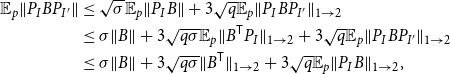 \begin{equation*} \begin{aligned} \mathbb {E}_p\|{P_I B P_{I'}}\| &\le \sqrt {\sigma }\mathbb {E}_p\|{P_I B}\| + 3\sqrt {q}\mathbb {E}_p\|{P_I B P_{I'}}\|_{1\rightarrow 2}\\ &\le \sigma \|{B}\| + 3\sqrt {q\sigma }\mathbb {E}_p\|{B^{\mathsf {T}} P_I}\|_{1\rightarrow 2} + 3\sqrt {q}\mathbb {E}_p\|{P_I B P_{I'}}\|_{1\rightarrow 2} \\ &\le \sigma \|{B}\| + 3\sqrt {q\sigma }\|{B^{\mathsf {T}}}\|_{1\rightarrow 2} + 3\sqrt {q}\mathbb {E}_p\|{P_I B}\|_{1\rightarrow 2}, \end{aligned} \end{equation*}
where the last inequality follows since the $1 \to 2$
norm of a submatrix is bounded by the
$1 \to 2$
norm of a submatrix is bounded by the $1 \to 2$
norm of a matrix. We then use Theorem6.5 to complete the proof:
$1 \to 2$
norm of a matrix. We then use Theorem6.5 to complete the proof:
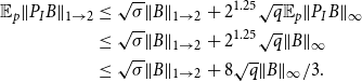 \begin{align*} \mathbb {E}_p\|P_I B\|_{1\rightarrow 2} &\le \sqrt {\sigma }\|{B}\|_{1\rightarrow 2} + 2^{1.25}\sqrt {q}\mathbb {E}_p\|{P_IB}\|_\infty \\ &\leq \sqrt {\sigma }\|{B}\|_{1\rightarrow 2} + 2^{1.25}\sqrt {q}\|{B}\|_\infty \\ &\leq \sqrt {\sigma }\|{B}\|_{1\rightarrow 2} + 8\sqrt {q}\|{B}\|_\infty /3. \end{align*}
Theorem6.3 gives a tool when one wishes to study the case of independent random subsets of row indices and column indices. However, because our goal is to study random subsets of fixed size of a given set, we cannot apply Theorem6.3 directly since now the selections of row indices and column indices are not independent. Instead, we would like to make $I=I'$
and change the model of sampling. The following tools make this possible.
$I=I'$
and change the model of sampling. The following tools make this possible.
Lemma 6.6 (Decoupling [Reference Tropp41]). Let $B$
be a diagonal-free symmetric
$B$
be a diagonal-free symmetric $n \times n$
matrix. Let
$n \times n$
matrix. Let $I,I' \sim \textrm {Subset}(n,\sigma )$
be two independent subsets, where
$I,I' \sim \textrm {Subset}(n,\sigma )$
be two independent subsets, where $\sigma \in (0,1)$
. Then for every
$\sigma \in (0,1)$
. Then for every $p \ge 2$
, we have
$p \ge 2$
, we have
 \begin{equation*}\mathbb {E}_p\|{P_I B P_I}\|\leq 2\mathbb {E}_p\|{P_I B P_{I'}}\|.\end{equation*}
Lemma 6.7 (Random subset models [Reference Tropp40]). Let $B$
be an
$B$
be an $n \times n$
matrix. Let
$n \times n$
matrix. Let $I \sim \textrm {Subset}(n,\sigma )$
and
$I \sim \textrm {Subset}(n,\sigma )$
and $J \sim \textrm {Subset}(n,m)$
be two independent subsets, where
$J \sim \textrm {Subset}(n,m)$
be two independent subsets, where $\sigma \in (0,1)$
and
$\sigma \in (0,1)$
and $m=\sigma n\ge 1$
. Then for every
$m=\sigma n\ge 1$
. Then for every $p\geq 2$
, we have
$p\geq 2$
, we have
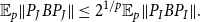 \begin{equation*} \mathbb {E}_p\|{P_J B P_J}\|\leq 2^{1/p}\mathbb {E}_p\|{P_I B P_I}\|. \end{equation*}
By combining the two lemmas above and Theorem6.3, we can obtain a corollary as follows:
Corollary 6.8 (Norms of random submatrices). Let $B$
be a symmetric
$B$
be a symmetric $n\times n$
matrix. Let
$n\times n$
matrix. Let $J \sim \textrm {Subset}(n,m)$
, where
$J \sim \textrm {Subset}(n,m)$
, where $\sigma \in (0,1)$
and
$\sigma \in (0,1)$
and $m=\sigma n\ge 1$
. Let
$m=\sigma n\ge 1$
. Let $p\geq 2$
and let
$p\geq 2$
and let $q=\max \{p,2\log n\}$
. Then
$q=\max \{p,2\log n\}$
. Then
 \begin{equation*} \mathbb {E}_p\|{P_J B P_J}\| \le 4\sigma \|{B}\| + 24\sqrt {q\sigma }\|{B}\|_{1\rightarrow 2} + 35q\|{B}\|_\infty . \end{equation*}
Proof.
Consider the symmetric, diagonal-free matrix $B_0=B-D$
where
$B_0=B-D$
where $D \,:\!=\, diag(B_{1,1},\ldots, B_{n,n})$
. Combining Theorem6.3 with Lemmas 6.6 and 6.7, we obtain the following:
$D \,:\!=\, diag(B_{1,1},\ldots, B_{n,n})$
. Combining Theorem6.3 with Lemmas 6.6 and 6.7, we obtain the following:
 \begin{equation*} \mathbb {E}_p\|{P_J B_0 P_J}\| \le 4\sigma \|{B_0}\| + 24\sqrt {q\sigma }\|{B_0}\|_{1\rightarrow 2} + 32q\|{B_0}\|_\infty . \end{equation*}
Note that $\|{B_0}\| \le \|{B}\|+\|{D}\|$
,
$\|{B_0}\| \le \|{B}\|+\|{D}\|$
, $\|{B_0}\|_{1\rightarrow 2} \le \|{B}\|_{1\rightarrow 2}$
,
$\|{B_0}\|_{1\rightarrow 2} \le \|{B}\|_{1\rightarrow 2}$
, $\|{B_0}\|_\infty \le \|{B}\|_\infty$
, and
$\|{B_0}\|_\infty \le \|{B}\|_\infty$
, and $\|{P_JBP_J}\| \le \|{P_JB_0P_J}\|+\|{P_JDP_J}\|\le \|{P_JB_0P_J}\|+\|{D}\|$
. This implies
$\|{P_JBP_J}\| \le \|{P_JB_0P_J}\|+\|{P_JDP_J}\|\le \|{P_JB_0P_J}\|+\|{D}\|$
. This implies
 \begin{equation*} \mathbb {E}_p\|{P_J B P_J}\| \leq \mathbb {E}_p\|{P_JB_0P_J}\| + \|{D}\| \le 4\sigma \left (\|{B}\|+\|{D}\|\right ) + 24\sqrt {q\sigma }\|{B}\|_{1\rightarrow 2} + 32q\|{B}\|_\infty + \|{D}\|. \end{equation*}
Notice that $\|{D}\|=\max _i|B_{i,i}| \le \|{B}\|_\infty$
to complete the proof.
$\|{D}\|=\max _i|B_{i,i}| \le \|{B}\|_\infty$
to complete the proof.
We are now ready to prove Theorem6.2.
Proof of Theorem
6.2
. Let $C\gt 0$
be a sufficiently large absolute constant. To see that the random induced subgraph
$C\gt 0$
be a sufficiently large absolute constant. To see that the random induced subgraph $H\,:\!=\, G[X]$
is almost regular whp, we can apply Lemma 6.1 with
$H\,:\!=\, G[X]$
is almost regular whp, we can apply Lemma 6.1 with $n,(1\pm \gamma )d,\sigma n,\gamma /(1+\gamma )$
in place of
$n,(1\pm \gamma )d,\sigma n,\gamma /(1+\gamma )$
in place of $N,K,n,a$
. Since
$N,K,n,a$
. Since $\sigma d\geq C\gamma ^{-2}\log n$
for sufficiently large absolute constant
$\sigma d\geq C\gamma ^{-2}\log n$
for sufficiently large absolute constant $C\gt 0$
, it follows that, with probability at least
$C\gt 0$
, it follows that, with probability at least $1-n^{-1}$
, all degrees of
$1-n^{-1}$
, all degrees of $H$
are
$H$
are $(1\pm 2\gamma )\sigma d$
. Thus, it remains to bound the second singular value of
$(1\pm 2\gamma )\sigma d$
. Thus, it remains to bound the second singular value of $A_H$
whp, where
$A_H$
whp, where $A_H$
is the adjacency matrix of
$A_H$
is the adjacency matrix of $H$
.
$H$
.
It is convenient to first work with normalised matrices. So let us consider the normalised adjacency matrix
 \begin{equation} \bar {A}_G=D^{-1/2}A_GD^{-1/2}, \quad \text {where} \quad D=diag(d_1,\ldots, d_n) \end{equation}
is the degree matrix of $G$
. Note that for any
$G$
. Note that for any $m\times n$
matrix
$m\times n$
matrix $A$
, we have that
$A$
, we have that $s_2(A)=\min _B\:\|{A-B}\|$
, where the minimum is over all rank-one
$s_2(A)=\min _B\:\|{A-B}\|$
, where the minimum is over all rank-one $m\times n$
matrices
$m\times n$
matrices $B$
(see Lemma A.4). Thus, by applying Observation 3.5, we have
$B$
(see Lemma A.4). Thus, by applying Observation 3.5, we have
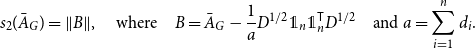 \begin{equation} s_2(\bar {A}_G)=\|{B}\|, \quad \text {where} \quad B = \bar {A}_G - \frac {1}{a} D^{1/2} \unicode {x1D7D9}_n \unicode {x1D7D9}_n^{\mathsf {T}} D^{1/2} \quad \text {and } a = \sum _{i=1}^n d_i. \end{equation}
Applying Corollary 6.8 for any $p\geq 2$
and
$p\geq 2$
and $q=\max \{p,2\log n\}$
, we obtain
$q=\max \{p,2\log n\}$
, we obtain
 \begin{equation} \mathbb {E}_p\|P_X B P_X\| \leq 4\sigma \|B\| + 24\sqrt {q\sigma }\|B\|_{1\rightarrow 2} + 35q\|{B}\|_\infty . \end{equation}
Let us bound each of the three terms on the right hand side.
Bounding $\|{B}\|$
. First, by (5), Corollary 4.2 and the assumptions, we have
$\|{B}\|$
. First, by (5), Corollary 4.2 and the assumptions, we have
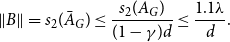 \begin{equation} \|{B}\| = s_2(\bar {A}_G) \le \frac {s_2(A_G)}{(1-\gamma )d} \leq \frac {1.1\lambda }{d}. \end{equation}
Bounding $\|{B}\|_{1\rightarrow 2}$
. Triangle inequality yields
$\|{B}\|_{1\rightarrow 2}$
. Triangle inequality yields
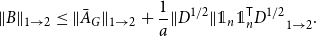 \begin{equation} \|B\|_{1\rightarrow 2} \le \|{\bar {A}_G}\|_{1\rightarrow 2} + \frac {1}{a} \|{D^{1/2}\| \unicode {x1D7D9}_n \unicode {x1D7D9}_n^{\mathsf {T}} D^{1/2}}_{1\rightarrow 2}. \end{equation}
Let us bound each of the terms appearing on the right-hand side. First,
 \begin{equation*} \|{\bar {A}_G}\|_{1\rightarrow 2} = \|{D^{-1/2}\|A_GD^{-1/2}}_{1\rightarrow 2} \le \|{D^{-1}}\| \|{A_G}\|_{1\rightarrow 2}. \end{equation*}
We have $\|{D^{-1}}\| = \max _i (1/d_i) \le 1.1/d$
and
$\|{D^{-1}}\| = \max _i (1/d_i) \le 1.1/d$
and $\|{A_G}\|_{1\rightarrow 2} = \max _j \sqrt {d_j} \le 1.1\sqrt {d}$
. Thus,
$\|{A_G}\|_{1\rightarrow 2} = \max _j \sqrt {d_j} \le 1.1\sqrt {d}$
. Thus,
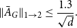 \begin{equation} \|{\bar {A}_G}\|_{1\rightarrow 2} \le \frac {1.3}{\sqrt {d}}. \end{equation}
Next,
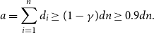 \begin{equation} a = \sum _{i=1}^n d_i\ge (1-\gamma )dn \ge 0.9dn. \end{equation}
Moreover,
 \begin{equation} \|{D^{1/2}\| \unicode {x1D7D9}_n \unicode {x1D7D9}_n^{\mathsf {T}} D^{1/2}}_{1\rightarrow 2} \le \|{D}\| \cdot \|{\unicode {x1D7D9}_n \unicode {x1D7D9}_n^{\mathsf {T}}}\|_{1\rightarrow 2} \le (1+\gamma )d \cdot \sqrt {n} \le 1.1d\sqrt {n}. \end{equation}
Putting (9), (10) and (11) into (8), we get
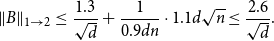 \begin{equation} \|B\|_{1\rightarrow 2} \le \frac {1.3}{\sqrt {d}} + \frac {1}{0.9dn} \cdot 1.1d\sqrt {n} \le \frac {2.6}{\sqrt {d}}. \end{equation}
Bounding $\|{B}\|_\infty$
. Again, triangle inequality yields
$\|{B}\|_\infty$
. Again, triangle inequality yields
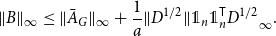 \begin{equation} \|B\|_\infty \le \|{\bar {A}_G}\|_\infty + \frac {1}{a} \|{D^{1/2}\| \unicode {x1D7D9}_n \unicode {x1D7D9}_n^{\mathsf {T}} D^{1/2}}_\infty . \end{equation}
All entries of $\bar {A}_G$
are
$\bar {A}_G$
are $1/\sqrt {d_id_j} \le 1.1/d$
, and all entries of
$1/\sqrt {d_id_j} \le 1.1/d$
, and all entries of $D^{1/2} \unicode {x1D7D9}_n \unicode {x1D7D9}_n^{\mathsf {T}} D^{1/2}$
are
$D^{1/2} \unicode {x1D7D9}_n \unicode {x1D7D9}_n^{\mathsf {T}} D^{1/2}$
are $\sqrt {d_id_j} \le 1.1d$
. Also, recall that
$\sqrt {d_id_j} \le 1.1d$
. Also, recall that $a \ge 0.9dn$
by (10). Thus, plugging them into (13), we obtain
$a \ge 0.9dn$
by (10). Thus, plugging them into (13), we obtain
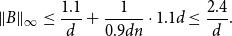 \begin{equation} \|{B}\|_\infty \le \frac {1.1}{d} + \frac {1}{0.9dn} \cdot 1.1d \le \frac {2.4}{d}. \end{equation}
Putting (7), (12) and (14) into (6), we obtain
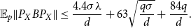 \begin{equation*} \mathbb {E}_p \|{P_X B P_X}\| \le \frac {4.4\sigma \lambda }{d} + 63\sqrt {\frac {q\sigma }{d}} + \frac {84q}{d}. \end{equation*}
Multiplying on the left and right by $D^{1/2}$
inside the norm, we conclude that
$D^{1/2}$
inside the norm, we conclude that
 \begin{equation*} \mathbb {E}_p \|{D^{1/2}\| P_X B P_X D^{1/2}} \le \|{D}\| \mathbb {E}_p \|{P_X B P_X}\| \le 5\sigma \lambda + 70\sqrt { q\sigma d} + 93q =: \lambda _0, \end{equation*}
where we used that $\|{D}\|=\max _i d_i \le 1.1d$
. Since diagonal matrices commute, we can express the matrix above as follows:
$\|{D}\|=\max _i d_i \le 1.1d$
. Since diagonal matrices commute, we can express the matrix above as follows:
 \begin{equation*} D^{1/2} P_X B P_X D^{1/2} = P_X D^{1/2} B D^{1/2} P_X = P_X A_G P_X - \frac {1}{a} P_X D \unicode {x1D7D9}_n \unicode {x1D7D9}_n^{\mathsf {T}} D P_X, \end{equation*}
where in the last step we used (4) and (5). Note that $\frac {1}{a} P_X D \unicode {x1D7D9}_n \unicode {x1D7D9}_n^{\mathsf {T}} D P_X$
is a rank one matrix. Thus, by Lemma A.4, we have
$\frac {1}{a} P_X D \unicode {x1D7D9}_n \unicode {x1D7D9}_n^{\mathsf {T}} D P_X$
is a rank one matrix. Thus, by Lemma A.4, we have $s_2(P_X A_G P_X) \le \|{D^{1/2}\| P_X B P_X D^{1/2}}$
, and thus
$s_2(P_X A_G P_X) \le \|{D^{1/2}\| P_X B P_X D^{1/2}}$
, and thus
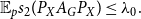 \begin{equation*} {\mathbb {E}}_p s_2(P_X A_G P_X) \le \lambda _0. \end{equation*}
Since the adjacency matrix $A_H$
of the induced subgraph
$A_H$
of the induced subgraph $H$
is a
$H$
is a $\sigma n\times \sigma n$
submatrix of the
$\sigma n\times \sigma n$
submatrix of the $n \times n$
matrix
$n \times n$
matrix $P_X A_G P_X$
, by the Interlacing Theorem for singular values (TheoremA.2), it follows that
$P_X A_G P_X$
, by the Interlacing Theorem for singular values (TheoremA.2), it follows that
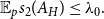 \begin{equation*} {\mathbb {E}}_p s_2(A_H) \le \lambda _0. \end{equation*}
Now choose $p=2\log n$
and thus
$p=2\log n$
and thus $q=p=2\log n$
. Applying Markov’s inequality, we obtain
$q=p=2\log n$
. Applying Markov’s inequality, we obtain
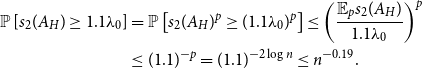 \begin{equation*}\begin{aligned} \mathbb {P} \left [ s_2(A_H) \ge 1.1\lambda _0 \right ] &= \mathbb {P} \left [ s_2(A_H)^p \ge (1.1\lambda _0)^p \right ] \le \left ( \frac {\mathbb {E}_p s_2(A_H)}{1.1\lambda _0}\right )^p \\ &\le (1.1)^{-p} =(1.1)^{-2\log n} \le n^{-0.19}. \end{aligned} \end{equation*}
In other words, with probability at least $1- n^{-0.19}$
, we have
$1- n^{-0.19}$
, we have
 \begin{equation*} s_2(A_H) \lt 1.1\lambda _0 \le 5.5\sigma \lambda + 109\sqrt { \sigma d\log n} + 205 \log n. \end{equation*}
To complete the proof, we show that the first term dominates the right-hand side. Indeed, since the absolute constant $C$
is sufficiently large, the first condition in Theorem6.2 implies that
$C$
is sufficiently large, the first condition in Theorem6.2 implies that $205 \log n \le \sqrt {\sigma d \log n}$
. Similarly, the second condition in the theorem implies that
$205 \log n \le \sqrt {\sigma d \log n}$
. Similarly, the second condition in the theorem implies that $110\sqrt { \sigma d\log n} \le 0.5 \sigma \lambda$
. Then it follows that
$110\sqrt { \sigma d\log n} \le 0.5 \sigma \lambda$
. Then it follows that
 \begin{equation*} s_2(A_H) \le 5.5\sigma \lambda + 0.5 \sigma \lambda = 6 \sigma \lambda . \end{equation*}
Therefore, with probability at least $(1-n^{-1})(1-n^{-0.19})\geq 1-n^{-1/6}$
,
$(1-n^{-1})(1-n^{-0.19})\geq 1-n^{-1/6}$
, $H$
is a
$H$
is a $\left (\sigma n, (1\pm 2\gamma )\sigma d, 6\sigma \lambda \right )$
-graph, which completes the proof of Theorem6.2.
$\left (\sigma n, (1\pm 2\gamma )\sigma d, 6\sigma \lambda \right )$
-graph, which completes the proof of Theorem6.2.
Sometimes we will work on the bipartite subgraph $G[X,Y]$
induced by random disjoint subsets
$G[X,Y]$
induced by random disjoint subsets $X,Y\subseteq V(G)$
. We also have
$X,Y\subseteq V(G)$
. We also have $G[X,Y]$
is a bipartite spectral expander whp, which is a direct corollary of Theorem6.2.
$G[X,Y]$
is a bipartite spectral expander whp, which is a direct corollary of Theorem6.2.
Corollary 6.9.
Let $\gamma \in (0,1/200]$
be a constant. There exists an absolute constant
$\gamma \in (0,1/200]$
be a constant. There exists an absolute constant $C$
such that the following holds for sufficiently large
$C$
such that the following holds for sufficiently large $n$
. Let
$n$
. Let $d,\lambda \gt 0$
, let
$d,\lambda \gt 0$
, let $\sigma _1,\sigma _2\in [1/n,1)$
, and let
$\sigma _1,\sigma _2\in [1/n,1)$
, and let $G$
be an
$G$
be an $(n,(1\pm \gamma )d,\lambda )$
-graph. Let
$(n,(1\pm \gamma )d,\lambda )$
-graph. Let $X,Y\subseteq V(G)$
with
$X,Y\subseteq V(G)$
with $|X|=\sigma _1 n$
and
$|X|=\sigma _1 n$
and $|Y|=\sigma _2n$
be two disjoint subsets chosen uniformly at random, and let
$|Y|=\sigma _2n$
be two disjoint subsets chosen uniformly at random, and let $H \,:\!=\, G[X,Y]$
be the bipartite subgraph of
$H \,:\!=\, G[X,Y]$
be the bipartite subgraph of $G$
induced by
$G$
induced by $X$
and
$X$
and $Y$
. Let
$Y$
. Let $\sigma \,:\!=\, \sigma _1+\sigma _2$
. Assume that
$\sigma \,:\!=\, \sigma _1+\sigma _2$
. Assume that
 \begin{equation*} \sigma _1d,\sigma _2 d\ge C \gamma ^{-2} \log n \quad \text {and} \quad \sigma \lambda \ge C\sqrt {\sigma d\log n}. \end{equation*}
Then with probability at least $1-n^{-1/7}$
,
$1-n^{-1/7}$
, $H$
is a
$H$
is a $\left (\sigma n, (1\pm 2\gamma )\sigma d, 6\sigma \lambda \right )$
-bipartite expander.
$\left (\sigma n, (1\pm 2\gamma )\sigma d, 6\sigma \lambda \right )$
-bipartite expander.
Proof.
Let $C\gt 0$
be a sufficiently large absolute constant. Since
$C\gt 0$
be a sufficiently large absolute constant. Since $\sigma _1n,\sigma _2n\geq C\gamma ^{-2}\log n$
, by Chernoff’s bounds, we have that
$\sigma _1n,\sigma _2n\geq C\gamma ^{-2}\log n$
, by Chernoff’s bounds, we have that
 \begin{equation*} \mathbb {P} \left [ \exists v\in V, \deg (v,X)\neq \left (1\pm 2\gamma \right )\sigma _1n \right ]\leq n^{-1} \end{equation*}
and
 \begin{equation*} \mathbb {P} \left [ \exists v\in V, \deg (v,Y)\neq \left (1\pm 2\gamma \right )\sigma _2n \right ]\leq n^{-1}. \end{equation*}
Next, note that $X\cup Y$
is a random subset of size
$X\cup Y$
is a random subset of size $|X|+|Y|=\sigma _1n+\sigma _2n=\sigma n$
. Now, since
$|X|+|Y|=\sigma _1n+\sigma _2n=\sigma n$
. Now, since $\sigma d=\sigma _1d+\sigma _2d\geq 2C\gamma ^{-2}\log n$
and
$\sigma d=\sigma _1d+\sigma _2d\geq 2C\gamma ^{-2}\log n$
and $\sigma \lambda \geq C\sqrt {\sigma d\log n}$
, Theorem6.2 implies that with probability at least
$\sigma \lambda \geq C\sqrt {\sigma d\log n}$
, Theorem6.2 implies that with probability at least $1-n^{-1/6}$
,
$1-n^{-1/6}$
,
 \begin{equation*} G[X\cup Y]\text { is a }\left (\sigma n,(1\pm 2\gamma )\sigma d,6\sigma \lambda \right )\text {-graph}. \end{equation*}
Therefore, we have that with probability at least $(1-2n^{-1})(1-n^{-1/6})\geq 1-n^{-1/7}$
,
$(1-2n^{-1})(1-n^{-1/6})\geq 1-n^{-1/7}$
,
 \begin{equation*} H\,:\!=\, G[X,Y]\text { is a }\left (\sigma n,(1\pm 2\gamma )\sigma d,6\sigma \lambda \right )\text {-bipartite expander}, \end{equation*}
which completes the proof.
7. Proof of Theorem1.2
In this section, we prove our main result, Theorem1.2. Since regular spectral expanders can be viewed as $(n, (1 \pm \gamma )d, \lambda )$
-graphs, the following slightly stronger statement will directly imply Theorem1.2.
$(n, (1 \pm \gamma )d, \lambda )$
-graphs, the following slightly stronger statement will directly imply Theorem1.2.
Theorem 7.1.
Let $\gamma \in (0,1/400]$
and let
$\gamma \in (0,1/400]$
and let $n$
be a sufficiently large integer. Then, any
$n$
be a sufficiently large integer. Then, any $(n,(1\pm \gamma )d,\lambda )$
-graph with
$(n,(1\pm \gamma )d,\lambda )$
-graph with $\lambda \leq d/70000$
and
$\lambda \leq d/70000$
and $d \geq \log ^{6}n$
contains a Hamilton cycle.
$d \geq \log ^{6}n$
contains a Hamilton cycle.
Before proving the theorem, we first state and prove the following simple averaging argument.
Claim 7.2.
Let $\alpha \in [0,1]$
, let
$\alpha \in [0,1]$
, let $0\lt m\leq h\leq n/2$
be integers, and let
$0\lt m\leq h\leq n/2$
be integers, and let $\mathcal {P}$
be any graph property. Let
$\mathcal {P}$
be any graph property. Let $G=(V,E)$
be a graph on
$G=(V,E)$
be a graph on $n$
vertices. Suppose that there are at least
$n$
vertices. Suppose that there are at least $1-\alpha$
proportion of pairs of disjoint
$1-\alpha$
proportion of pairs of disjoint $m$
-sets
$m$
-sets $A,B\subseteq V$
such that
$A,B\subseteq V$
such that $G[A,B]\in \mathcal {P}$
. Let
$G[A,B]\in \mathcal {P}$
. Let $\mathcal {F}\subseteq \binom Vm$
be the family of
$\mathcal {F}\subseteq \binom Vm$
be the family of $m$
-sets
$m$
-sets $A$
such that for at least
$A$
such that for at least $1-\alpha ^{1/2}$
proportion of
$1-\alpha ^{1/2}$
proportion of $m$
-sets
$m$
-sets $B\subseteq V\setminus A$
,
$B\subseteq V\setminus A$
, $G[A,B]\in \mathcal {P}$
. For
$G[A,B]\in \mathcal {P}$
. For $A\in \mathcal F$
, let
$A\in \mathcal F$
, let $\mathcal F_A\subseteq \binom {V\setminus A}m$
be the family of
$\mathcal F_A\subseteq \binom {V\setminus A}m$
be the family of $m$
-sets
$m$
-sets $B\subseteq V\setminus A$
such that
$B\subseteq V\setminus A$
such that $G[A,B]\in \mathcal {P}$
. Then the following properties hold:
$G[A,B]\in \mathcal {P}$
. Then the following properties hold:
-
(A1)
$|\mathcal {F}|\ge (1-\alpha ^{1/2})\binom {n}{m}$
; -
(A2) for a uniformly random
$h$
-set
$S\subseteq V\setminus A$
, with probability at least
$1-\alpha ^{1/4}$
,
$|\mathcal F_A\cap \binom Sm|\ge (1-\alpha ^{1/4})\binom hm$
; -
(A3) for
$A\in \binom Vm$
and
$S\in \binom Vh$
chosen uniformly at random such that
$A\cap S=\emptyset$
, with probability at least
$1-\alpha ^{1/2}-\alpha ^{1/4}$
, for at least
$1-\alpha ^{1/4}$
proportion of
$m$
-sets
$B\subseteq S$
,
$G[A,B]\in \mathcal {P}$
.


Proof. We prove the statements in sequence.
Property (A1). Suppose to the contrary that there are at least $\alpha ^{1/2}\binom {n}{m}$ $m$
-sets
$m$
-sets $A\notin \mathcal {F}$
. By definition, each such
$A\notin \mathcal {F}$
. By definition, each such $A$
contributes at least
$A$
contributes at least $\alpha ^{1/2}\binom {n-m}{m}$
pairs
$\alpha ^{1/2}\binom {n-m}{m}$
pairs $(A,B)$
such that
$(A,B)$
such that $G[A,B]\notin \mathcal {P}$
. Therefore, there are at least
$G[A,B]\notin \mathcal {P}$
. Therefore, there are at least $\alpha ^{1/2}\binom {n}{m}\cdot \alpha ^{1/2}\binom {n-m}{m} = \alpha \binom {n}{m}\binom {n-m}{m}$
pairs
$\alpha ^{1/2}\binom {n}{m}\cdot \alpha ^{1/2}\binom {n-m}{m} = \alpha \binom {n}{m}\binom {n-m}{m}$
pairs $(A,B)$
such that
$(A,B)$
such that $G[A,B]\notin \mathcal {P}$
, contradicting the assumption that there are at least
$G[A,B]\notin \mathcal {P}$
, contradicting the assumption that there are at least $1-\alpha$
proportion of pairs
$1-\alpha$
proportion of pairs $(A,B)$
with
$(A,B)$
with $G[A,B]\in \mathcal {P}$
. Thus,
$G[A,B]\in \mathcal {P}$
. Thus, $|\mathcal {F}|\ge (1-\alpha ^{1/2})\binom {n}{m}$
.
$|\mathcal {F}|\ge (1-\alpha ^{1/2})\binom {n}{m}$
.
Property (A2). Suppose to the contrary that there are more than $\alpha ^{1/4}\binom {n-m}{h}$ $h$
-sets
$h$
-sets $S\subseteq V\setminus A$
, each containing at least
$S\subseteq V\setminus A$
, each containing at least $\alpha ^{1/4}\binom {h}{m}$ $m$
-sets
$m$
-sets $B$
such that
$B$
such that $B\notin \mathcal {F}_A$
. Since each such subset
$B\notin \mathcal {F}_A$
. Since each such subset $B$
is counted at most
$B$
is counted at most $\binom {n-2m}{h-m}$
times, there are in total more than
$\binom {n-2m}{h-m}$
times, there are in total more than
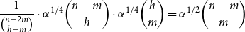 \begin{equation*} \frac {1}{\binom {n-2m}{h-m}}\cdot \alpha ^{1/4}\binom {n-m}{h}\cdot \alpha ^{1/4}\binom {h}{m} = \alpha ^{1/2}\binom {n-m}{m} \end{equation*} $m$
-sets
$m$
-sets $B$
such that
$B$
such that $B\notin \mathcal {F}_A$
. This contradicts the assumption that
$B\notin \mathcal {F}_A$
. This contradicts the assumption that $|\mathcal F_A|\ge (1-\alpha ^{1/2})\binom {n-m}{m}$
.
$|\mathcal F_A|\ge (1-\alpha ^{1/2})\binom {n-m}{m}$
.
Property (A3). By applying (A1), (A2), and the union bound, for disjoint uniformly randomly chosen $A\in \binom Vm$
and
$A\in \binom Vm$
and $S\in \binom Vh$
, with probability at least
$S\in \binom Vh$
, with probability at least $1-\alpha ^{1/2}-\alpha ^{1/4}$
, we have that
$1-\alpha ^{1/2}-\alpha ^{1/4}$
, we have that $A\in \mathcal F$
and
$A\in \mathcal F$
and $|\mathcal F_A\cap \binom Sm|\ge (1-\alpha ^{1/4})\binom hm$
. This implies that for at least
$|\mathcal F_A\cap \binom Sm|\ge (1-\alpha ^{1/4})\binom hm$
. This implies that for at least $1-\alpha ^{1/4}$
proportion of
$1-\alpha ^{1/4}$
proportion of $m$
-sets
$m$
-sets $B\subseteq S$
,
$B\subseteq S$
, $G[A,B]\in \mathcal {P}$
.
$G[A,B]\in \mathcal {P}$
.
The proof is completed.
We are now ready to prove Theorem7.1.
Proof of Theorem
7.1
. Assume that $\gamma \leq 1/400$
,
$\gamma \leq 1/400$
, $\lambda \leq d/70000$
, and that
$\lambda \leq d/70000$
, and that $G=(V,E)$
is an
$G=(V,E)$
is an $(n,(1\pm \gamma )d,\lambda )$
-graph with a sufficiently large integer
$(n,(1\pm \gamma )d,\lambda )$
-graph with a sufficiently large integer $n$
and
$n$
and $d\geq \log ^6n$
. Since an
$d\geq \log ^6n$
. Since an $(n,(1\pm \gamma )d,\lambda )$
-graph is also an
$(n,(1\pm \gamma )d,\lambda )$
-graph is also an $(n,(1\pm \gamma )d,\lambda ')$
-graph when
$(n,(1\pm \gamma )d,\lambda ')$
-graph when $\lambda \leq \lambda '$
, we may assume that
$\lambda \leq \lambda '$
, we may assume that $\sqrt {d}\log ^3n\leq \lambda \leq d/70000$
. Let
$\sqrt {d}\log ^3n\leq \lambda \leq d/70000$
. Let $k\,:\!=\, n/\log ^4n$
.
$k\,:\!=\, n/\log ^4n$
.
7.1 Partitioning the graph
First, we find a partition of the vertex set of the $(n,(1\pm \gamma )d,\lambda )$
-graph
$(n,(1\pm \gamma )d,\lambda )$
-graph $G$
with some nice properties.
$G$
with some nice properties.
Claim 7.3.
There exists a partition $V=X_1\cup X_2\cup Y_1\cup Y_2\cup R_1\cup R_2$
with
$V=X_1\cup X_2\cup Y_1\cup Y_2\cup R_1\cup R_2$
with $|X_1|=|Y_1|=\frac {k}{5}$
,
$|X_1|=|Y_1|=\frac {k}{5}$
, $|X_2|=|Y_2|=\frac {4k}{5}$
and
$|X_2|=|Y_2|=\frac {4k}{5}$
and $|R_2|=\frac {4n}{5}$
, such that the following properties hold:
$|R_2|=\frac {4n}{5}$
, such that the following properties hold:
-
(P1) for every vertex
$v\in V$
, we have:
\begin{equation*} \begin{aligned} \deg (v,X_1),\deg (v,Y_1)&= (1\pm 2\gamma )\frac {dk}{5n},\quad \deg (v,X_2),\deg (v,Y_2)= (1\pm 2\gamma )\frac {4dk}{5n}\\ \deg (v,R_1)&=(1\pm 2\gamma )\frac {d}{5},\quad \text {and}\quad \deg (v,R_2)=(1\pm 2\gamma )\frac {4d}{5}; \end{aligned} \end{equation*}
-
(P2) letting
$X\,:\!=\, X_1\cup X_2$
and
$Y\,:\!=\, Y_1\cup Y_2$
, the subgraph
\begin{equation*} G'\,:\!=\, G[X\cup Y\cup R_1]\text { is an }\left (\frac {n}{5},(1\pm 2\gamma )\frac {d}{5}, \frac {6\lambda }{5}\right )\text {-graph}; \end{equation*}
-
(P3) for at least
$1-n^{-1/7}$
proportion of disjoint subsets
$S,T\subseteq R_1\cup R_2$
of equal size
$k$
,
\begin{equation*} G[S,T]\text { is a }\left (2k,(1\pm 4\gamma )\frac {2dk}{n},\frac {18\lambda k}{n}\right )\text {-bipartite expander}; \end{equation*}
-
(P4) for at least
$1-n^{-1/28}$
proportion of
$k$
-sets
$S\subseteq R_1\cup R_2$
, the bipartite subgraphs
\begin{equation*}G[X,S]\text { and }G[S,Y]\text { are }\left (2k,(1\pm 2\gamma )\frac {2dk}{n},\frac {12\lambda k}{n}\right )\text{-}bipartite\ expanders; \end{equation*}
-
(P5) the bipartite subgraph
\begin{equation*} G[X,Y]\text { is a }\left (2k,(1\pm 2\gamma )\frac {2dk}{n}, \frac {12\lambda k}{n}\right )\text{-}bipartite\ expander. \end{equation*}


Proof of Claim 7.3
. Let $V=X_1\cup X_2\cup Y_1\cup Y_2\cup R_1\cup R_2$
be a uniformly random partition with
$V=X_1\cup X_2\cup Y_1\cup Y_2\cup R_1\cup R_2$
be a uniformly random partition with $|X_1|=|Y_1|=\frac {k}{5}$
,
$|X_1|=|Y_1|=\frac {k}{5}$
, $|X_2|=|Y_2|=\frac {4k}{5}$
and
$|X_2|=|Y_2|=\frac {4k}{5}$
and $|R_2|=\frac {4n}{5}$
. We wish to prove that each property among (P1)–(P5) holds whp.
$|R_2|=\frac {4n}{5}$
. We wish to prove that each property among (P1)–(P5) holds whp.
Property (P1). Since for all $v\in V$
we have
$v\in V$
we have $\mathbb {E}[\deg (v,X_1)]=(1\pm \gamma )\frac {dk}{5n}=\omega (\log n)$
, it follows by Chernoff’s bounds and the union bound that
$\mathbb {E}[\deg (v,X_1)]=(1\pm \gamma )\frac {dk}{5n}=\omega (\log n)$
, it follows by Chernoff’s bounds and the union bound that
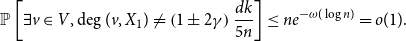 \begin{equation*} \mathbb {P} \left [ \exists v\in V, \deg (v,X_1)\neq \left (1\pm 2\gamma \right )\frac {dk}{5n} \right ]\leq ne^{-\omega (\log n)}=o(1). \end{equation*}
Similarly, the other degree bounds also hold with probability at least $1 - o(1)$
. Therefore, property (P1) holds with high probability. For the remainder of the proof, we will condition on property (P1).
$1 - o(1)$
. Therefore, property (P1) holds with high probability. For the remainder of the proof, we will condition on property (P1).
Property (P2). Note that $X\cup Y\cup R_1$
is a uniformly random subset of size
$X\cup Y\cup R_1$
is a uniformly random subset of size $\frac {n}{5}$
. Since
$\frac {n}{5}$
. Since $\frac {d}{5}=\omega (\gamma ^{-2}\log n)$
and
$\frac {d}{5}=\omega (\gamma ^{-2}\log n)$
and $\frac {\lambda }{5}=\omega \left (\sqrt {\frac {d\log n}{5}}\right )$
, by Theorem6.2, we have that with probability at least
$\frac {\lambda }{5}=\omega \left (\sqrt {\frac {d\log n}{5}}\right )$
, by Theorem6.2, we have that with probability at least $1-n^{-1/6}$
,
$1-n^{-1/6}$
,
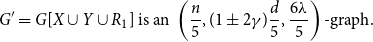 \begin{equation*} G'= G[X\cup Y\cup R_1]\text { is an }\left (\frac {n}{5},(1\pm 2\gamma )\frac {d}{5}, \frac {6\lambda }{5}\right )\text {-graph}. \end{equation*}
Property (P3). First, we prove that $G[R_1\cup R_2]$
is an
$G[R_1\cup R_2]$
is an $(n-2k,(1\pm \frac {3}{2}\gamma )d,\lambda )$
-graph. Indeed, by property (P1), for every vertex
$(n-2k,(1\pm \frac {3}{2}\gamma )d,\lambda )$
-graph. Indeed, by property (P1), for every vertex $v\in V$
,
$v\in V$
,
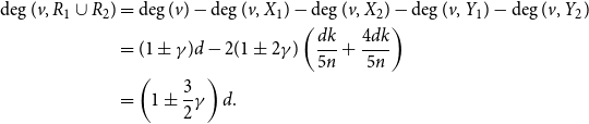 \begin{equation*} \begin{aligned} \deg (v,R_1\cup R_2)&= \deg (v)-\deg (v,X_1)-\deg (v,X_2)-\deg (v,Y_1)-\deg (v,Y_2)\\ &=(1\pm \gamma )d-2(1\pm 2\gamma )\left (\frac {dk}{5n}+\frac {4dk}{5n}\right )\\ &=\left (1\pm \frac {3}{2}\gamma \right )d. \end{aligned} \end{equation*}
Also, by the Interlacing Theorem for singular values (TheoremA.2), we have that $s_2(G[R_1\cup R_2])\leq s_2(G)\leq \lambda$
. Therefore,
$s_2(G[R_1\cup R_2])\leq s_2(G)\leq \lambda$
. Therefore, $G[R_1\cup R_2]$
is an
$G[R_1\cup R_2]$
is an $(n-2k,(1\pm \frac {3}{2}\gamma )d,\lambda )$
-graph.
$(n-2k,(1\pm \frac {3}{2}\gamma )d,\lambda )$
-graph.
Next, let $S,T\subseteq R_1\cup R_2$
be two disjoint
$S,T\subseteq R_1\cup R_2$
be two disjoint $k$
-sets chosen uniformly at random. Since
$k$
-sets chosen uniformly at random. Since $(1+\frac {1}{2}\gamma )\frac {2dk}{n}\geq \frac {2dk}{n-2k}=\omega ((2\gamma )^{-2}\log n)$
and
$(1+\frac {1}{2}\gamma )\frac {2dk}{n}\geq \frac {2dk}{n-2k}=\omega ((2\gamma )^{-2}\log n)$
and $ \frac {3\lambda k}{n}\geq \frac {2\lambda k}{n-2k}=\omega \left (\sqrt {\frac {2dk\log n}{n-2k}}\right )$
, Theorem6.2 implies that with probability at least
$ \frac {3\lambda k}{n}\geq \frac {2\lambda k}{n-2k}=\omega \left (\sqrt {\frac {2dk\log n}{n-2k}}\right )$
, Theorem6.2 implies that with probability at least $1-n^{-1/6}$
,
$1-n^{-1/6}$
,
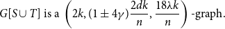 \begin{equation*} G[S\cup T]\text { is a }\left (2k,(1\pm 4\gamma )\frac {2dk}{n},\frac {18\lambda k}{n}\right )\text {-graph}. \end{equation*}
Also, by Chernoff’s bounds, with probability at least (say) $1-n^{-1}$
, for every vertex
$1-n^{-1}$
, for every vertex $v\in V$
,
$v\in V$
,
 \begin{equation*} \deg (v,S),\deg (v,T)=(1\pm 4\gamma )\frac {dk}{n}. \end{equation*}
Thus, by the union bound, for at least $(1- n^{-1/6})(1- n^{-1})\geq 1- n^{-1/7}$
proportion of disjoint subsets
$(1- n^{-1/6})(1- n^{-1})\geq 1- n^{-1/7}$
proportion of disjoint subsets $S,T\subseteq R_1\cup R_2$
of equal size
$S,T\subseteq R_1\cup R_2$
of equal size $k$
,
$k$
,
 \begin{equation*} G[S,T]\text { is a }\left (2k,(1\pm 4\gamma )\frac {2dk}{n},\frac {18\lambda k}{n}\right )\text {-bipartite expander.} \end{equation*}
Property (P4). We only prove the property for $X$
, while the analogous statement for
$X$
, while the analogous statement for $Y$
can be shown similarly. By applying Corollary 6.9, we can obtain that for at least
$Y$
can be shown similarly. By applying Corollary 6.9, we can obtain that for at least $1-n^{-1/7}$
proportion of disjoint subsets
$1-n^{-1/7}$
proportion of disjoint subsets $A,B\subseteq V$
of equal size
$A,B\subseteq V$
of equal size $k$
,
$k$
,
 \begin{equation*} G[A,B]\text { is a }\left (2k,(1\pm 2\gamma )\frac {2dk}{n},\frac {12\lambda k}{n}\right )\text {-bipartite expander}. \end{equation*}
Note that $X$
is a uniformly random
$X$
is a uniformly random $k$
-set and
$k$
-set and $R_1\cup R_2\subseteq V\setminus X$
is a uniformly random
$R_1\cup R_2\subseteq V\setminus X$
is a uniformly random $(n-2k)$
-set. Thus, by (A3) applied with
$(n-2k)$
-set. Thus, by (A3) applied with $X,R_1\cup R_2,k,n-2k,n^{-1/7}$
in place of
$X,R_1\cup R_2,k,n-2k,n^{-1/7}$
in place of $A,S,m,h,\alpha$
, we have that with probability at least
$A,S,m,h,\alpha$
, we have that with probability at least $1-n^{-1/14}-n^{-1/28}\geq 1-n^{-1/29}$
, for at least
$1-n^{-1/14}-n^{-1/28}\geq 1-n^{-1/29}$
, for at least $1-n^{-1/28}$
proportion of
$1-n^{-1/28}$
proportion of $k$
-sets
$k$
-sets $S\subseteq R_1\cup R_2$
,
$S\subseteq R_1\cup R_2$
,
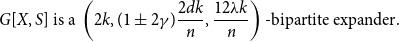 \begin{equation*} G[X,S]\text { is a }\left (2k,(1\pm 2\gamma )\frac {2dk}{n},\frac {12\lambda k}{n}\right )\text {-bipartite expander}. \end{equation*}
Property (P5). Note that $X\cup Y$
is a uniformly random subset of size
$X\cup Y$
is a uniformly random subset of size $2k$
. Since
$2k$
. Since $\frac {2dk}{n}=\omega (\gamma ^{-2}\log n)$
and
$\frac {2dk}{n}=\omega (\gamma ^{-2}\log n)$
and $\frac {2\lambda k}{n}=\omega \left (\sqrt {\frac {2dk\log n}{n}}\right )$
, by Theorem6.2, we have that with probability at least
$\frac {2\lambda k}{n}=\omega \left (\sqrt {\frac {2dk\log n}{n}}\right )$
, by Theorem6.2, we have that with probability at least $1-n^{-1/6}$
,
$1-n^{-1/6}$
,
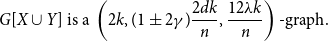 \begin{equation*} G[X\cup Y]\text { is a }\left (2k,(1\pm 2\gamma )\frac {2dk}{n}, \frac {12\lambda k}{n}\right )\text {-graph}. \end{equation*}
Now by (Q1), the bipartite subgraph
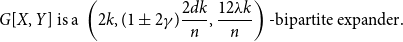 \begin{equation*} G[X,Y]\text { is a }\left (2k,(1\pm 2\gamma )\frac {2dk}{n}, \frac {12\lambda k}{n}\right )\text {-bipartite expander}. \end{equation*}
All in all, with positive probability all properties (P1)–(P5) hold, which guarantees a partition $V=X_1\cup X_2\cup Y_1\cup Y_2\cup R_1\cup R_2$
satisfying all desired properties. This completes the proof.
$V=X_1\cup X_2\cup Y_1\cup Y_2\cup R_1\cup R_2$
satisfying all desired properties. This completes the proof.
7.2 Finding
$S_{res}$
and partitioning
$(R_1\cup R_2)\setminus V(S_{res})$


We pick a partition $V=X_1\cup X_2\cup Y_1\cup Y_2\cup R_1\cup R_2$
as in Claim 7.3. In order to find the subgraph
$V=X_1\cup X_2\cup Y_1\cup Y_2\cup R_1\cup R_2$
as in Claim 7.3. In order to find the subgraph $S_{res}$
which will be used to close a collection of vertex-disjoint paths into a cycle, we first verify the assumptions of Lemma 5.3. Recall that
$S_{res}$
which will be used to close a collection of vertex-disjoint paths into a cycle, we first verify the assumptions of Lemma 5.3. Recall that $G'=G[X\cup Y\cup R_1]$
. Let
$G'=G[X\cup Y\cup R_1]$
. Let $D\,:\!=\, \frac {d}{700\lambda }\geq 100$
, and let
$D\,:\!=\, \frac {d}{700\lambda }\geq 100$
, and let $m\,:\!=\, \frac {(1+2\gamma )^2}{(1-2\gamma )^3}\cdot \frac {(6\lambda /5)\cdot (n/5)}{d/5}+1\leq \frac {2\lambda n}{d}$
.
$m\,:\!=\, \frac {(1+2\gamma )^2}{(1-2\gamma )^3}\cdot \frac {(6\lambda /5)\cdot (n/5)}{d/5}+1\leq \frac {2\lambda n}{d}$
.
Claim 7.4. The following properties hold:
-
1.
$G'$
is
$m$
-joined;
-
2.
$I(X\cup Y)$
is
$(D,m)$
-extendable in
$G'$
.


Proof of Claim 7.4
. Recall that by (P2), $G'$
is an
$G'$
is an $(\frac {n}{5},(1\pm 2\gamma )\frac {d}{5}, \frac {6\lambda }{5})$
-graph. Corollary 4.4 implies that
$(\frac {n}{5},(1\pm 2\gamma )\frac {d}{5}, \frac {6\lambda }{5})$
-graph. Corollary 4.4 implies that $G'$
is
$G'$
is $m$
-joined, so we are left to prove (2). In fact, since
$m$
-joined, so we are left to prove (2). In fact, since $I(X\cup Y)$
is an empty graph,
$I(X\cup Y)$
is an empty graph, $\Delta (I(X\cup Y))=0\leq D$
. Also, recall that by (P1), for every vertex
$\Delta (I(X\cup Y))=0\leq D$
. Also, recall that by (P1), for every vertex $v\in V$
,
$v\in V$
, $\deg _G(v,R_1)\geq (1-2\gamma )\frac {d}{5}\geq \frac {d}{6}$
. Since
$\deg _G(v,R_1)\geq (1-2\gamma )\frac {d}{5}\geq \frac {d}{6}$
. Since $G$
is an
$G$
is an $(n,(1\pm \gamma )d,\lambda )$
-graph, by Lemma 4.5, we have that for any subset
$(n,(1\pm \gamma )d,\lambda )$
-graph, by Lemma 4.5, we have that for any subset $U\subseteq V(G')$
of size
$U\subseteq V(G')$
of size $1\leq |U|\leq 2m\leq \frac {4\lambda n}{d}$
,
$1\leq |U|\leq 2m\leq \frac {4\lambda n}{d}$
,
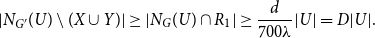 \begin{equation*} |N_{G'}(U)\setminus (X\cup Y)|\geq |N_{G}(U)\cap R_1|\geq \frac {d}{700\lambda }|U|=D|U|. \end{equation*}
Thus, by Proposition 5.2, $I(X\cup Y)$
is
$I(X\cup Y)$
is $(D,m)$
-extendable in
$(D,m)$
-extendable in $G'$
. This completes the proof.
$G'$
. This completes the proof.
Now, let $C\gt 0$
be the constant in Lemma 5.3, and let
$C\gt 0$
be the constant in Lemma 5.3, and let $\ell \,:\!=\,\lfloor C\log ^3(\frac {n}{5})\rfloor$
. Since
$\ell \,:\!=\,\lfloor C\log ^3(\frac {n}{5})\rfloor$
. Since $D\geq 100$
and
$D\geq 100$
and $m\leq \frac {n/5}{100D}$
, by applying Lemma 5.3 on
$m\leq \frac {n/5}{100D}$
, by applying Lemma 5.3 on $G'$
with
$G'$
with $\frac {n}{5},\frac {\log ^4 n}{5\log ^3(n/5)},X,Y$
in place of
$\frac {n}{5},\frac {\log ^4 n}{5\log ^3(n/5)},X,Y$
in place of $n,K,V_1,V_2$
, we can find a subgraph
$n,K,V_1,V_2$
, we can find a subgraph $S_{res}\subseteq G'=G[X\cup Y\cup R_1]$
with
$S_{res}\subseteq G'=G[X\cup Y\cup R_1]$
with $|V(S_{res})|=k\ell$
satisfying the conclusion of the lemma.
$|V(S_{res})|=k\ell$
satisfying the conclusion of the lemma.
Assuming without loss of generality that $|R_1\cup R_2|$
is divisible by
$|R_1\cup R_2|$
is divisible by $k$
, we further partition
$k$
, we further partition $R_1\cup R_2$
into
$R_1\cup R_2$
into $k$
-sets, each of which has a small intersection with
$k$
-sets, each of which has a small intersection with $S_{res}$
, and every pair of such sets induces a bipartite expander. For convenience, we will let
$S_{res}$
, and every pair of such sets induces a bipartite expander. For convenience, we will let $V_1\,:\!=\, X$
and
$V_1\,:\!=\, X$
and $V_t\,:\!=\, Y$
for the remainder of the proof, where
$V_t\,:\!=\, Y$
for the remainder of the proof, where $t\,:\!=\, \frac {n-2k}{k}$
.
$t\,:\!=\, \frac {n-2k}{k}$
.
Claim 7.5. There exists a partition
 \begin{equation*} R_1\cup R_2=V_2\cup \ldots \cup V_{t-1} \end{equation*}
into $k$
-sets such that the following properties hold:
$k$
-sets such that the following properties hold:
-
(Q1) for each
$2\leq i\leq t-1$
, we have
$|V_i\setminus V(S_{res})|\geq k-\frac {2Ck}{\log n}$
; -
(Q2) for each
$2\leq i\leq t-1$
,
$|V_{i,1}|=(1\pm \gamma )\frac {k}{5}$
and
$|V_{i,2}|=(1\pm \gamma )\frac {4k}{5}$
, where
$V_{i,1}\,:\!=\, V_i\cap R_1$
and
$V_{i,2}\,:\!=\, V_i\cap R_2$
; -
(Q3) for each
$2\leq i\leq t-1$
and for every vertex
$v\in V$
, we have
\begin{equation*}\deg (v,V_{i,1})=(1\pm 5\gamma )\frac {dk}{5n} \textrm { and } \deg (v,V_{i,2})=(1\pm 5\gamma )\frac {4dk}{5n};\end{equation*}
-
(Q4) for each distinct
$i,j\in [t]$
, the subgraph
\begin{equation*} G[V_i,V_j]\text { is a }\left (2k,(1\pm 5\gamma )\frac {2dk}{n},\frac {18\lambda k}{n}\right )\text {-bipartite expander}; \end{equation*}
-
(Q5) for each distinct
$i,j\in [t]$
, the bipartite subgraph
where
\begin{equation*} G[V_{i,1},V_{j,1}]\text { is a }\left (|V_{i,1}|+|V_{j,1}|,(1\pm 5\gamma )\frac {2dk}{5n},\frac {18\lambda k}{n}\right )\text {-bipartite expander,} \end{equation*}
$V_{1,1}\,:\!=\, X_1$
and
$V_{t,1}\,:\!=\, Y_1$
.


Proof of Claim 7.5. Let $ R_1\cup R_2=V_2\cup \ldots \cup V_{t-1}$
be a uniformly random partition into
$ R_1\cup R_2=V_2\cup \ldots \cup V_{t-1}$
be a uniformly random partition into $k$
-sets. We wish to prove that each property among (Q1)–(Q5) holds whp.
$k$
-sets. We wish to prove that each property among (Q1)–(Q5) holds whp.
Property (Q1). Recall that $|S_{res}|=k\ell =\frac {n}{\log ^4n}\cdot C\log ^3(\frac {n}{5})$
. Since for each
$|S_{res}|=k\ell =\frac {n}{\log ^4n}\cdot C\log ^3(\frac {n}{5})$
. Since for each $2\leq i\leq t-1$
,
$2\leq i\leq t-1$
, $V_i$
is a uniformly random
$V_i$
is a uniformly random $k$
-set, we have that
$k$
-set, we have that $\mathbb {E}[|V_i\cap S_{res}|]=\frac {k}{\log ^4n}\cdot C\log ^3(\frac {n}{5})$
. Thus, by Chernoff’s bounds and the union bound,
$\mathbb {E}[|V_i\cap S_{res}|]=\frac {k}{\log ^4n}\cdot C\log ^3(\frac {n}{5})$
. Thus, by Chernoff’s bounds and the union bound,
 \begin{equation*} \mathbb {P} \left [ |V_i\cap S_{res}|\geq \frac {2Ck}{\log n}\text { for some }2\leq i\leq t-1 \right ]\leq te^{-\Theta \left (\frac {Ck}{\log n}\right )}=o(1). \end{equation*}
Therefore, property (Q1) holds with probability $1-o(1)$
.
$1-o(1)$
.
Property (Q2). Recall that $|R_1|=\frac {n}{5}-2k$
and
$|R_1|=\frac {n}{5}-2k$
and $|R_2|=\frac {4n}{5}$
. Since
$|R_2|=\frac {4n}{5}$
. Since $V_i$
is chosen as a uniformly random
$V_i$
is chosen as a uniformly random $k$
-set, we have
$k$
-set, we have $\mathbb {E}[|V_{i,1}|]=\frac {k}{5}-\frac {2k^2}{n}$
and
$\mathbb {E}[|V_{i,1}|]=\frac {k}{5}-\frac {2k^2}{n}$
and $\mathbb {E}[|V_{i,2}|]=\frac {4k}{5}$
. By applying Chernoff’s bounds and the union bound, we get
$\mathbb {E}[|V_{i,2}|]=\frac {4k}{5}$
. By applying Chernoff’s bounds and the union bound, we get
 \begin{equation*} \mathbb {P} \left [ |V_{i,1}|\neq (1\pm \gamma )\frac {k}{5}\text { or }|V_{i,2}|\neq (1\pm \gamma )\frac {4k}{5}\text { for some }2\leq i\leq t-1 \right ]\leq te^{-\omega (\log n)}=o(1), \end{equation*}
where the last inequality holds since $k=\omega (\log n)$
. Thus, property (Q2) holds with probability
$k=\omega (\log n)$
. Thus, property (Q2) holds with probability $1-o(1)$
. For the remainder of the proof, we will condition on property (Q2).
$1-o(1)$
. For the remainder of the proof, we will condition on property (Q2).
Property (Q3). Recall from property (P1) that for every vertex $v\in V$
, we have
$v\in V$
, we have $\deg (v,R_1)=(1\pm 2\gamma )\frac {d}{5}$
. Additionally, by (Q2), for each
$\deg (v,R_1)=(1\pm 2\gamma )\frac {d}{5}$
. Additionally, by (Q2), for each $2\leq i\leq t-1$
,
$2\leq i\leq t-1$
, $V_{i,1}$
is a random subset of size
$V_{i,1}$
is a random subset of size $(1\pm \gamma )\frac {k}{5}$
. Now, conditioning on
$(1\pm \gamma )\frac {k}{5}$
. Now, conditioning on $|V_{i,1}|=a=(1\pm \gamma )\frac {k}{5}$
,
$|V_{i,1}|=a=(1\pm \gamma )\frac {k}{5}$
, $\deg (v,V_{i,1})$
is a hypergeometric random variable with expectation
$\deg (v,V_{i,1})$
is a hypergeometric random variable with expectation $(1\pm 2\gamma )\frac {da}{n}=(1\pm 4\gamma )\frac {dk}{5n}$
. Thus, fixing
$(1\pm 2\gamma )\frac {da}{n}=(1\pm 4\gamma )\frac {dk}{5n}$
. Thus, fixing $v\in V$
and
$v\in V$
and $2\leq i\leq t-1$
, Chernoff’s bounds imply that
$2\leq i\leq t-1$
, Chernoff’s bounds imply that
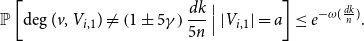 \begin{equation*} \mathbb {P} \left [ \deg (v,V_{i,1})\neq \left (1\pm 5\gamma \right )\frac {dk}{5n}\,\Big |\,|V_{i,1}|=a \right ] \leq e^{-\omega (\frac {dk}{n})}. \end{equation*}
By the law of total probability and the union bound, we obtain that
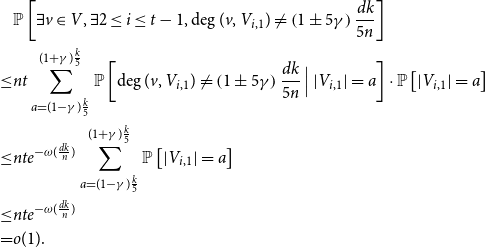 \begin{equation*} \begin{aligned} &\mathbb {P} \left [ \exists v\in V,\exists 2\leq i\leq t-1,\deg (v,V_{i,1})\neq \left (1\pm 5\gamma \right )\frac {dk}{5n} \right ]\\ \leq & nt\sum _{a=(1-\gamma )\frac {k}{5}}^{(1+\gamma )\frac {k}{5}}\mathbb {P} \left [ \deg (v,V_{i,1})\neq \left (1\pm 5\gamma \right )\frac {dk}{5n}\,\Big |\,|V_{i,1}|=a \right ]\cdot \mathbb {P} \left [ |V_{i,1}|=a \right ]\\ \leq & nte^{-\omega (\frac {dk}{n})}\sum _{a=(1-\gamma )\frac {k}{5}}^{(1+\gamma )\frac {k}{5}}\mathbb {P} \left [ |V_{i,1}|=a \right ]\\ \leq & nte^{-\omega (\frac {dk}{n})}\\ =& o(1). \end{aligned} \end{equation*}
Therefore, with an analogous proof for $\deg (v,V_{i,2})$
, property (Q3) holds with probability
$\deg (v,V_{i,2})$
, property (Q3) holds with probability $1-o(1)$
.
$1-o(1)$
.
Property (Q4). First, recall that by (P5), $G[X,Y]$
is a
$G[X,Y]$
is a $\left (2k,(1\pm 2\gamma )\frac {2dk}{n},\frac {12\lambda k}{n}\right )$
-bipartite expander. Next, recall that by (P3), for two random disjoint
$\left (2k,(1\pm 2\gamma )\frac {2dk}{n},\frac {12\lambda k}{n}\right )$
-bipartite expander. Next, recall that by (P3), for two random disjoint $k$
-sets
$k$
-sets $V_i,V_j\subseteq R_1\cup R_2$
chosen uniformly at random, with probability at least
$V_i,V_j\subseteq R_1\cup R_2$
chosen uniformly at random, with probability at least $1-n^{-1/7}$
,
$1-n^{-1/7}$
, $G[V_i,V_j]$
is a
$G[V_i,V_j]$
is a $\left (2k,(1\pm 4\gamma )\frac {2dk}{n},\frac {18\lambda k}{n}\right )$
-bipartite expander. Thus, by the union bound, with probability at least
$\left (2k,(1\pm 4\gamma )\frac {2dk}{n},\frac {18\lambda k}{n}\right )$
-bipartite expander. Thus, by the union bound, with probability at least $1-\binom {t-2}{2}n^{-1/7}$
, for each pair
$1-\binom {t-2}{2}n^{-1/7}$
, for each pair $2\leq i\lt j\leq t-1$
,
$2\leq i\lt j\leq t-1$
, $G[V_i,V_j]$
is a
$G[V_i,V_j]$
is a $\left (2k,(1\pm 4\gamma )\frac {2dk}{n},\frac {18\lambda k}{n}\right )$
-bipartite expander.
$\left (2k,(1\pm 4\gamma )\frac {2dk}{n},\frac {18\lambda k}{n}\right )$
-bipartite expander.
Finally, recall that by (P4), for a random $k$
-sets
$k$
-sets $V_i\subseteq R_1\cup R_2$
chosen uniformly at random, with probability at least
$V_i\subseteq R_1\cup R_2$
chosen uniformly at random, with probability at least $1-n^{-1/28}$
,
$1-n^{-1/28}$
, $G[X,V_i]$
and
$G[X,V_i]$
and $G[V_i,Y]$
are
$G[V_i,Y]$
are $\left (2k,(1\pm 2\gamma )\frac {2dk}{n},\frac {12\lambda k}{n}\right )$
-bipartite expanders. Again, by the union bound, with probability at least
$\left (2k,(1\pm 2\gamma )\frac {2dk}{n},\frac {12\lambda k}{n}\right )$
-bipartite expanders. Again, by the union bound, with probability at least $1-(t-2)n^{-1/28}$
, for each
$1-(t-2)n^{-1/28}$
, for each $2\leq i\leq t-1$
,
$2\leq i\leq t-1$
, $G[X,V_i]$
and
$G[X,V_i]$
and $G[V_i,Y]$
are
$G[V_i,Y]$
are $\left (2k,(1\pm 4\gamma )\frac {2dk}{n},\frac {18\lambda k}{n}\right )$
-bipartite expanders.
$\left (2k,(1\pm 4\gamma )\frac {2dk}{n},\frac {18\lambda k}{n}\right )$
-bipartite expanders.
Therefore, in total, (Q4) holds with probability at least
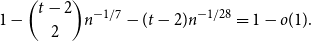 \begin{equation*} 1-\binom {t-2}{2}n^{-1/7}-(t-2)n^{-1/28}=1-o(1). \end{equation*}
For the remainder of the proof, we will condition on property (Q3) and (Q4).
Property (Q5). Recall that by (P1) and (Q3), we have that for each $i\in [t]$
and for every vertex
$i\in [t]$
and for every vertex $v\in V$
,
$v\in V$
, $\deg (v,V_{i,1})=(1\pm 5\gamma )\frac {dk}{5n}$
. Also, recall that (Q4) implies that
$\deg (v,V_{i,1})=(1\pm 5\gamma )\frac {dk}{5n}$
. Also, recall that (Q4) implies that $s_2(G[V_i\cup V_j])\leq \frac {18\lambda k}{n}$
. Thus, by the Interlacing Theorem for singular values (TheoremA.2),
$s_2(G[V_i\cup V_j])\leq \frac {18\lambda k}{n}$
. Thus, by the Interlacing Theorem for singular values (TheoremA.2), $s_2(G[V_{i,1}\cup V_{j,1}])\leq s_2(G[V_i\cup V_j])\leq \frac {18\lambda k}{n}$
. Therefore,
$s_2(G[V_{i,1}\cup V_{j,1}])\leq s_2(G[V_i\cup V_j])\leq \frac {18\lambda k}{n}$
. Therefore,
 \begin{equation*} G[V_{i,1},V_{j,1}]\text { is a }\left (|V_{i,1}|+|V_{j,1}|,(1\pm 5\gamma )\frac {2dk}{5n},\frac {18\lambda k}{n}\right )\text {-bipartite expander.} \end{equation*}
All in all, with positive probability all properties (Q1)–(Q5) hold, which guarantees a partition $R_1\cup R_2=V_2\cup \ldots \cup V_{t-1}$
satisfying all desired properties. This completes the proof.
$R_1\cup R_2=V_2\cup \ldots \cup V_{t-1}$
satisfying all desired properties. This completes the proof.
7.3 Finding vertex-disjoint paths
We pick a partition $R_1\cup R_2=V_2\cup \ldots \cup V_{t-1}$
as in Claim 7.5, and let
$R_1\cup R_2=V_2\cup \ldots \cup V_{t-1}$
as in Claim 7.5, and let $U_i\,:\!=\, V_i\setminus V(S_{res})$
for each
$U_i\,:\!=\, V_i\setminus V(S_{res})$
for each $2\leq i\leq t-1$
. Also, denote
$2\leq i\leq t-1$
. Also, denote $U_1\,:\!=\, V_1$
for simplicity in the iterative process defined below. By reordering if necessary, without loss of generality, we may assume that
$U_1\,:\!=\, V_1$
for simplicity in the iterative process defined below. By reordering if necessary, without loss of generality, we may assume that $|U_1|\geq |U_2|\geq \ldots \geq |U_{t-1}|,$
and let
$|U_1|\geq |U_2|\geq \ldots \geq |U_{t-1}|,$
and let $n_1\geq n_2\geq \ldots \geq n_{t-1}$
be the corresponding sizes of the
$n_1\geq n_2\geq \ldots \geq n_{t-1}$
be the corresponding sizes of the $|U_i|$
s. We wish to find vertex-disjoint paths covering all the vertices in
$|U_i|$
s. We wish to find vertex-disjoint paths covering all the vertices in $\bigcup _{i=1}^{t-1} U_i\cup V_t$
, where each path has one endpoint in
$\bigcup _{i=1}^{t-1} U_i\cup V_t$
, where each path has one endpoint in $U_1=X$
and the other in
$U_1=X$
and the other in $V_t=Y$
. Note that if all the
$V_t=Y$
. Note that if all the $n_i$
s were the same, then we could simply find perfect matchings between each pair
$n_i$
s were the same, then we could simply find perfect matchings between each pair $U_i$
and
$U_i$
and $U_{i+1}$
. Since the
$U_{i+1}$
. Since the $n_i$
s are not the same, we will first use Lemma 4.8 to find vertex-disjoint matchings
$n_i$
s are not the same, we will first use Lemma 4.8 to find vertex-disjoint matchings $M_i$
s, where
$M_i$
s, where $M_i$
is a matching of size
$M_i$
is a matching of size $n_i-n_{i+1}$
between
$n_i-n_{i+1}$
between $U_i$
and
$U_i$
and $V_t$
. Then, noticing that the remainder of each two consecutive parts have the same size, we will apply Lemma 4.7 to find a perfect matching
$V_t$
. Then, noticing that the remainder of each two consecutive parts have the same size, we will apply Lemma 4.7 to find a perfect matching $N_i$
between the remainder of each two consecutive parts. Now, concatenating all the matchings
$N_i$
between the remainder of each two consecutive parts. Now, concatenating all the matchings $M_i$
s and
$M_i$
s and $N_i$
s will give the desired vertex-disjoint paths (see Figure. 1 for illustration).
$N_i$
s will give the desired vertex-disjoint paths (see Figure. 1 for illustration).
Initially, let $V_t'\,:\!=\, V_t$
. First, we find a matching
$V_t'\,:\!=\, V_t$
. First, we find a matching $M_1$
of size
$M_1$
of size $n_1-n_2$
between
$n_1-n_2$
between $U_1\cap V_{1,1}$
and
$U_1\cap V_{1,1}$
and $V_t'\cap V_{t,1}$
. Recall that we have
$V_t'\cap V_{t,1}$
. Recall that we have $n_1-n_2\leq \frac {2Ck}{\log n}$
by (Q1). Also, recall that by (Q5),
$n_1-n_2\leq \frac {2Ck}{\log n}$
by (Q1). Also, recall that by (Q5),
 \begin{equation*} G[V_{1,1},V_{t,1}]\text { is a }\left (|V_{1,1}|+|V_{t,1}|,(1\pm 5\gamma )\frac {2dk}{5n},\frac {18\lambda k}{n}\right )\text {-bipartite expander.} \end{equation*}
Thus, by Lemma 4.8, there exists a matching $M_1$
of size
$M_1$
of size $n_1-n_{2}$
in
$n_1-n_{2}$
in $G$
between
$G$
between $U_1\cap V_{1,1}$
and
$U_1\cap V_{1,1}$
and $V_t'\cap V_{t,1}$
. Let
$V_t'\cap V_{t,1}$
. Let $U_1'\,:\!=\, U_1\setminus V(M_1)$
and
$U_1'\,:\!=\, U_1\setminus V(M_1)$
and $V_t'\,:\!=\, V_t'\setminus V(M_1)$
. Now, we have that
$V_t'\,:\!=\, V_t'\setminus V(M_1)$
. Now, we have that $|U_1'|=|U_2|=n_2$
, which is necessary to find a perfect matching between
$|U_1'|=|U_2|=n_2$
, which is necessary to find a perfect matching between $U_1'$
and
$U_1'$
and $U_2$
. Also,
$U_2$
. Also, $|V_t'|=n_2$
.
$|V_t'|=n_2$
.
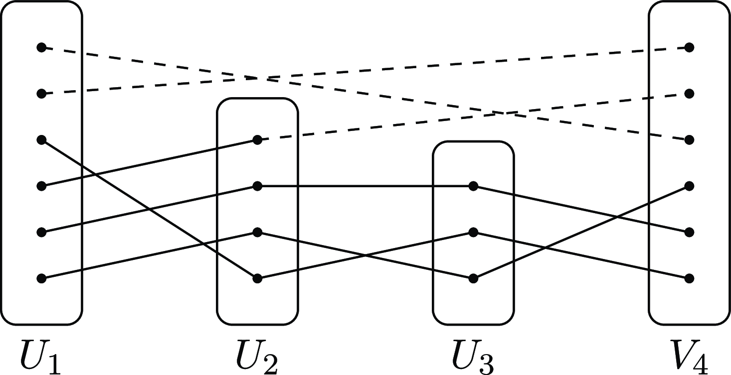
Figure 1. The figure is an example for connecting the matchings into vertex-disjoint paths when $t=4$
. The dashed lines represent matchings
$t=4$
. The dashed lines represent matchings $M_i$
s, and the straight lines represent matchings
$M_i$
s, and the straight lines represent matchings $N_i$
s.
$N_i$
s.
Next, we find a matching $M_2$
of size
$M_2$
of size $n_2-n_3$
between
$n_2-n_3$
between $U_2\cap V_{2,1}$
and
$U_2\cap V_{2,1}$
and $V_t'\cap V_{t,1}$
. Recall that by (Q1), we have
$V_t'\cap V_{t,1}$
. Recall that by (Q1), we have
 \begin{equation*} |V_{2,1}\setminus U_2|+(n_2-n_3)=|V_{t,1}\setminus V_t'|+(n_2-n_3)=n_1-n_3\leq \frac {2Ck}{\log n} \end{equation*}
Also, recall that by (Q5),
 \begin{equation*} G[V_{2,1},V_{t,1}]\text { is a }\left (|V_{2,1}|+|V_{t,1}|,(1\pm 5\gamma )\frac {2dk}{5n},\frac {18\lambda k}{n}\right )\text {-bipartite expander.} \end{equation*}
Thus, by Lemma 4.8, there exists a matching $M_2$
of size
$M_2$
of size $n_2-n_{3}$
in
$n_2-n_{3}$
in $G$
between
$G$
between $U_2\cap V_{2,1}$
and
$U_2\cap V_{2,1}$
and $V_t'\cap V_{t,1}$
. Let
$V_t'\cap V_{t,1}$
. Let $U_2'\,:\!=\, U_2\setminus V(M_2)$
and
$U_2'\,:\!=\, U_2\setminus V(M_2)$
and $V_t'\,:\!=\, V_t'\setminus V(M_2)$
. Now, we have that
$V_t'\,:\!=\, V_t'\setminus V(M_2)$
. Now, we have that $|U_2'|=|U_3|=n_3$
, which is necessary to find a perfect matching between
$|U_2'|=|U_3|=n_3$
, which is necessary to find a perfect matching between $U_2'$
and
$U_2'$
and $U_3$
. Also,
$U_3$
. Also, $|V_t'|=n_3$
. Continuing in this fashion, we can and do find vertex-disjoint matchings
$|V_t'|=n_3$
. Continuing in this fashion, we can and do find vertex-disjoint matchings $M_i$
s between
$M_i$
s between $U_i$
and
$U_i$
and $V_t$
for each
$V_t$
for each $i\in [t-2]$
. And crucially, we have that
$i\in [t-2]$
. And crucially, we have that $|U_i'|=|U_{i+1}|=n_{i+1}$
for each
$|U_i'|=|U_{i+1}|=n_{i+1}$
for each $i\in [t-2]$
, and
$i\in [t-2]$
, and $|U_{t-1}|=|V_{t}'|=n_{t-1}$
. In the rest of proof, we let
$|U_{t-1}|=|V_{t}'|=n_{t-1}$
. In the rest of proof, we let $U_{t-1}'\,:\!=\, U_{t-1}$
and
$U_{t-1}'\,:\!=\, U_{t-1}$
and $U_t\,:\!=\, V_t'$
for simplicity of the following iterative process.
$U_t\,:\!=\, V_t'$
for simplicity of the following iterative process.
Now, we find a perfect matching between $U_i'$
and
$U_i'$
and $U_{i+1}$
for each
$U_{i+1}$
for each $i\in [t-1]$
. To do so, we first prove that the induced bipartite subgraph
$i\in [t-1]$
. To do so, we first prove that the induced bipartite subgraph $G[U_i',U_{i+1}]$
is a bipartite expander. Recall that for each
$G[U_i',U_{i+1}]$
is a bipartite expander. Recall that for each $i\in [t-1]$
,
$i\in [t-1]$
, $G[V_i,V_{i+1}]$
is a
$G[V_i,V_{i+1}]$
is a $\left (2k,(1\pm 5\gamma )\frac {2dk}{n},\frac {18\lambda k}{n}\right )$
-bipartite expander by (Q4). So for every vertex
$\left (2k,(1\pm 5\gamma )\frac {2dk}{n},\frac {18\lambda k}{n}\right )$
-bipartite expander by (Q4). So for every vertex $v\in V_i\cup V_{i+1}$
,
$v\in V_i\cup V_{i+1}$
,
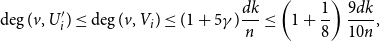 \begin{equation*} \deg (v,U_i')\leq \deg (v,V_i)\leq (1+5\gamma )\frac {dk}{n}\leq \left (1+\frac {1}{8}\right )\frac {9dk}{10n}, \end{equation*}
and
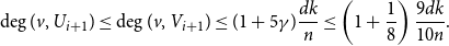 \begin{equation*} \deg (v,U_{i+1})\leq \deg (v,V_{i+1})\leq (1+5\gamma )\frac {dk}{n}\leq \left (1+\frac {1}{8}\right )\frac {9dk}{10n}. \end{equation*}
Also, recall that by (Q3), for every vertex $v\in V_i\cup V_{i+1}$
,
$v\in V_i\cup V_{i+1}$
, $\deg (v,V_{i,2}),\deg (v,V_{i+1,2})=(1\pm 5\gamma )\frac {4dk}{5n}$
. Since
$\deg (v,V_{i,2}),\deg (v,V_{i+1,2})=(1\pm 5\gamma )\frac {4dk}{5n}$
. Since $V_{i,2}\subseteq U_i'$
and
$V_{i,2}\subseteq U_i'$
and $V_{i+1,2}\subseteq U_{i+1}$
for each
$V_{i+1,2}\subseteq U_{i+1}$
for each $i\in [t-1]$
, this implies that
$i\in [t-1]$
, this implies that
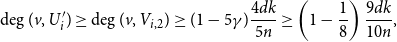 \begin{equation*} \deg (v,U_i')\geq \deg (v,V_{i,2})\geq (1-5\gamma )\frac {4dk}{5n}\geq \left (1-\frac {1}{8}\right )\frac {9dk}{10n}, \end{equation*}
and
 \begin{equation*} \deg (v,U_{i+1})\geq \deg (v,V_{i+1,2})\geq (1-5\gamma )\frac {4dk}{5n}\geq \left (1-\frac {1}{8}\right )\frac {9dk}{10n}, \end{equation*}
where we used $\gamma \leq 1/400$
in the last step of both inequalities. Finally, by the Interlacing Theorem for singular values (TheoremA.2),
$\gamma \leq 1/400$
in the last step of both inequalities. Finally, by the Interlacing Theorem for singular values (TheoremA.2), $s_2(G[U_i'\cup U_{i+1}])\leq s_2(G[V_i\cup V_{i+1}])\leq \frac {18\lambda k}{n}$
. Therefore,
$s_2(G[U_i'\cup U_{i+1}])\leq s_2(G[V_i\cup V_{i+1}])\leq \frac {18\lambda k}{n}$
. Therefore,
 \begin{equation*} G[U_i', U_{i+1}]\text { is a }\left (|U_i'|+|U_{i+1}|,\left (1\pm \frac {1}{8}\right )\frac {9dk}{5n},\frac {18\lambda k}{n}\right )\text {-bipartite expander}. \end{equation*}
Thus, since $\frac {18\lambda k}{n}\leq \frac {1}{200}\cdot \frac {9dk}{5n}$
, by Lemma 4.7, there exists a perfect matching
$\frac {18\lambda k}{n}\leq \frac {1}{200}\cdot \frac {9dk}{5n}$
, by Lemma 4.7, there exists a perfect matching $N_i$
in
$N_i$
in $G$
between
$G$
between $U_i'$
and
$U_i'$
and $U_{i+1}$
. Now, by concatenating all the matchings
$U_{i+1}$
. Now, by concatenating all the matchings $M_i$
s and
$M_i$
s and $N_i$
s together, we obtain vertex-disjoint paths
$N_i$
s together, we obtain vertex-disjoint paths $P_1,\ldots, P_k$
covering
$P_1,\ldots, P_k$
covering $\bigcup _{i=1}^{t-1} U_i\cup V_t$
, where each path has one endpoint in
$\bigcup _{i=1}^{t-1} U_i\cup V_t$
, where each path has one endpoint in $U_1=X$
and the other in
$U_1=X$
and the other in $V_t=Y$
.
$V_t=Y$
.
7.4 Closing paths into a cycle
Let $a_i\in X$
and
$a_i\in X$
and $b_i\in Y$
be the endpoints of the path
$b_i\in Y$
be the endpoints of the path $P_i$
. Now, Lemma 5.3 implies that
$P_i$
. Now, Lemma 5.3 implies that $S_{res}$
has a path-factor
$S_{res}$
has a path-factor $Q_1,\ldots, Q_k$
such that
$Q_1,\ldots, Q_k$
such that $Q_i$
connects
$Q_i$
connects $b_{i}$
and
$b_{i}$
and $a_{i+1}$
, where
$a_{i+1}$
, where $a_{t+1}\,:\!=\, a_1$
. Therefore,
$a_{t+1}\,:\!=\, a_1$
. Therefore, $P_1Q_1P_2Q_2\ldots P_kQ_k$
is a Hamilton cycle of
$P_1Q_1P_2Q_2\ldots P_kQ_k$
is a Hamilton cycle of $G$
. This completes the proof.
$G$
. This completes the proof.
Acknowledgements
Part of this work was done when Jie Han visited the math department of UCI in spring 2023, and he would like to thank the department for the hospitality. We would like to thank an anonymous referee whose careful reading and valuable suggestions helped us improve the paper considerably. In particular, we thank the referee for suggesting the result from [20] which replaces the absorption method and simplifies our proof significantly.
In this definition and elsewhere in the paper, we write $a = b \pm c$
as a shorthand for the double-sided inequality
$a = b \pm c$
as a shorthand for the double-sided inequality $b-c \le a \le b+c$
. We use other similar abbreviations, whose exact meaning should be clear from context.
$b-c \le a \le b+c$
. We use other similar abbreviations, whose exact meaning should be clear from context.
A.F. was partially supported by NSF grant DMS-1953799, NSF Career DMS-2146406, a Sloan’s fellowship, and an Air force grant FA9550-23-1-0298. J.H. was partially supported by Natural Science Foundation of China (12371341). R.V. was partially supported by NSF grant DMS-1954233, NSF grant DMS-2027299, U.S. Army grant 76649-CS, and NSF+Simons Research Collaborations on the Mathematical and Scientific Foundations of Deep Learning.
A. Linear algebra background
In this section we collect some standard tools from linear algebra.
The following theorem provides a convenient tool for computing/bounding eigenvalues of a real symmetric matrix (see for example Theorem 2.4.1 in [6]).
Theorem A.1 (Courant-Fischer Minimax Theorem). Let $A$
be a symmetric
$A$
be a symmetric $n\times n$
matrix with eigenvalues
$n\times n$
matrix with eigenvalues $\lambda _1\geq \lambda _2\geq \ldots \geq \lambda _n$
. Then,
$\lambda _1\geq \lambda _2\geq \ldots \geq \lambda _n$
. Then,
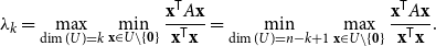 \begin{equation*} \lambda _k=\max _{\dim (U)=k}\min _{\mathbf {x}\in U\setminus \{\mathbf {0}\}}\frac {\mathbf {x}^{\mathsf {T}} A\mathbf {x}}{\mathbf {x}^{\mathsf {T}}\mathbf {x}}=\min _{\dim (U)=n-k+1}\max _{\mathbf {x}\in U\setminus \{\mathbf {0}\}}\frac {\mathbf {x}^{\mathsf {T}} A\mathbf {x}}{\mathbf {x}^{\mathsf {T}}\mathbf {x}}. \end{equation*}
Since the notion of eigenvalues is undefined for non-square matrices, it would be convenient for us to work with singular values which are defined for all matrices (see Definition 3.3). The following theorem proved by Thompson [39] is useful when one wants to obtain non-trivial bounds on the singular values of submatrices.
Theorem A.2 (Interlacing Theorem for singular values). Let $A$
be an
$A$
be an $m\times n$
matrix and let
$m\times n$
matrix and let
 \begin{equation*}\alpha _1\geq \alpha _2\geq \ldots \geq \alpha _{\min \{m,n\}}\end{equation*}
be its singular values. Let $B$
be any
$B$
be any $p\times q$
submatrix of
$p\times q$
submatrix of $A$
and let
$A$
and let
 \begin{equation*}\beta _1\geq \beta _2\geq \ldots \geq \beta _{\min \{p,q\}}\end{equation*}
be its singular values. Then
 \begin{equation*} \begin{aligned} \alpha _i\geq \beta _i,\quad \quad \quad \quad \quad \quad \:\:&\text {for }i=1,2,\ldots, \min \{p,q\},\\ \beta _i\geq \alpha _{i+(m-p)+(n-q)},\quad &\text {for }i\leq \min \{p+q-m,p+q-n\}. \end{aligned} \end{equation*}
One of the most commonly used tools in linear algebra is the singular value decomposition. We need a slightly stronger version of it, which almost immediately follows from the standard proof:
Theorem A.3 (Singular value decomposition). Let $M$
be an
$M$
be an $m\times n$
matrix with rank
$m\times n$
matrix with rank $r$
. Let
$r$
. Let $s_1\geq s_2\geq \ldots \geq s_r$
be all the positive singular values of
$s_1\geq s_2\geq \ldots \geq s_r$
be all the positive singular values of $M$
. Let
$M$
. Let $\mathbf {u}_1\in {\mathbb {R}}^m$
and
$\mathbf {u}_1\in {\mathbb {R}}^m$
and ${\mathbf {v}}_1\in {\mathbb {R}}^n$
be unit vectors such that
${\mathbf {v}}_1\in {\mathbb {R}}^n$
be unit vectors such that $M{\mathbf {v}}_1=s_1\mathbf {u}_1$
. Then we can find an orthonormal bases
$M{\mathbf {v}}_1=s_1\mathbf {u}_1$
. Then we can find an orthonormal bases $\{\mathbf {u}_1,\ldots, \mathbf {u}_m\}$
of
$\{\mathbf {u}_1,\ldots, \mathbf {u}_m\}$
of ${\mathbb {R}}^m$
and
${\mathbb {R}}^m$
and $\{{\mathbf {v}}_1,\ldots, {\mathbf {v}}_n\}$
of
$\{{\mathbf {v}}_1,\ldots, {\mathbf {v}}_n\}$
of ${\mathbb {R}}^n$
with
${\mathbb {R}}^n$
with $\mathbf {u}_1$
and
$\mathbf {u}_1$
and ${\mathbf {v}}_1$
as above, and such that
${\mathbf {v}}_1$
as above, and such that
 \begin{equation*}M=\sum _{j=1}^rs_j\mathbf {u}_j{\mathbf {v}}_j^{\mathsf {T}}.\end{equation*}
In particular, this equality implies that $M{\mathbf {v}}_j=s_j\mathbf {u}_j$
for
$M{\mathbf {v}}_j=s_j\mathbf {u}_j$
for $j=1,\ldots, r$
and
$j=1,\ldots, r$
and $M{\mathbf {v}}_j=\mathbf {0}$
for
$M{\mathbf {v}}_j=\mathbf {0}$
for $j\gt r$
.
$j\gt r$
.
We will also make use of the following simple corollary of the above theorem, which proof is included for completion.
Lemma A.4 (Best low-rank approximation). Let $A$
be an
$A$
be an $m \times n$
matrix. Then
$m \times n$
matrix. Then
 \begin{equation*} s_2(A)=\min _B\:\|{A-B}\|, \end{equation*}
where the minimum is over all rank-one $m\times n$
matrices
$m\times n$
matrices $B$
, and
$B$
, and $\|{\mkern 2mu\cdot \mkern 2mu}\|$
denotes the operator norm.
$\|{\mkern 2mu\cdot \mkern 2mu}\|$
denotes the operator norm.
Moreover, the minimum is attained by $B = s_1(A)\mathbf {u}_1{\mathbf {v}}^{\mathsf {T}}_1$
, where
$B = s_1(A)\mathbf {u}_1{\mathbf {v}}^{\mathsf {T}}_1$
, where ${\mathbf {v}}_1\in {\mathbb {R}}^n$
and
${\mathbf {v}}_1\in {\mathbb {R}}^n$
and $\mathbf {u}_1\in {\mathbb {R}}^m$
are any unit vectors such that
$\mathbf {u}_1\in {\mathbb {R}}^m$
are any unit vectors such that $A{\mathbf {v}}_1=s_1(A)\mathbf {u}_1$
.
$A{\mathbf {v}}_1=s_1(A)\mathbf {u}_1$
.
Proof.
Let $A$
be an
$A$
be an $m \times n$
matrix with rank
$m \times n$
matrix with rank $r$
. Let
$r$
. Let $s_1\geq s_2\geq \ldots \geq s_r$
be all positive singular values of
$s_1\geq s_2\geq \ldots \geq s_r$
be all positive singular values of $A$
, and let
$A$
, and let ${\mathbf {v}}_1\in {\mathbb {R}}^n$
and
${\mathbf {v}}_1\in {\mathbb {R}}^n$
and $\mathbf {u}_1\in {\mathbb {R}}^m$
be unit vectors such that
$\mathbf {u}_1\in {\mathbb {R}}^m$
be unit vectors such that $A{\mathbf {v}}_1=s_1\mathbf {u}_1$
. By TheoremA.3, there exist orthonormal bases
$A{\mathbf {v}}_1=s_1\mathbf {u}_1$
. By TheoremA.3, there exist orthonormal bases $\{{\mathbf {v}}_1,\ldots, {\mathbf {v}}_n\}$
of
$\{{\mathbf {v}}_1,\ldots, {\mathbf {v}}_n\}$
of ${\mathbb {R}}^n$
and
${\mathbb {R}}^n$
and $\{\mathbf {u}_1,\ldots, \mathbf {u}_m\}$
of
$\{\mathbf {u}_1,\ldots, \mathbf {u}_m\}$
of ${\mathbb {R}}^m$
, such that
${\mathbb {R}}^m$
, such that
 \begin{equation*}A=\sum _{j=1}^rs_j\mathbf {u}_j{\mathbf {v}}_j^{\mathsf {T}}. \end{equation*}
First, note that $B=s_1{\mathbf {u}}_1{\mathbf {v}}_1^{\mathsf {T}}$
is a rank-one matrix that satisfies
$B=s_1{\mathbf {u}}_1{\mathbf {v}}_1^{\mathsf {T}}$
is a rank-one matrix that satisfies
 \begin{equation*} \|{A-B}\| =\|\sum _{j=2}^r s_j{\mathbf {u}}_j{\mathbf {v}}_j^{\mathsf {T}}\| =s_2. \end{equation*}
Therefore, to finish the proof, it suffices to show $s_2\leq \|A-B\|$
for every rank-one
$s_2\leq \|A-B\|$
for every rank-one $m\times n$
matrix
$m\times n$
matrix $B$
. We can express such a matrix as
$B$
. We can express such a matrix as $B=\mathbf {x}\mathbf {y}^{\mathsf {T}}$
for some nonzero vectors
$B=\mathbf {x}\mathbf {y}^{\mathsf {T}}$
for some nonzero vectors $\mathbf {x} \in \mathbb {R}^m$
and
$\mathbf {x} \in \mathbb {R}^m$
and $\mathbf {y} \in {\mathbb {R}}^n$
. Next, we can find a nontrivial linear combination
$\mathbf {y} \in {\mathbb {R}}^n$
. Next, we can find a nontrivial linear combination $\mathbf {w}=a{\mathbf {v}}_1+b{\mathbf {v}}_2$
such that
$\mathbf {w}=a{\mathbf {v}}_1+b{\mathbf {v}}_2$
such that $\langle \mathbf {y},\mathbf {w} \rangle = \mathbf {0}$
; this implies
$\langle \mathbf {y},\mathbf {w} \rangle = \mathbf {0}$
; this implies $B\mathbf {w}=\mathbf {x}(\mathbf {y}^{\mathsf {T}}\mathbf {w})=0$
. Without loss of generality, we can scale
$B\mathbf {w}=\mathbf {x}(\mathbf {y}^{\mathsf {T}}\mathbf {w})=0$
. Without loss of generality, we can scale $\mathbf {w}$
so that
$\mathbf {w}$
so that $\|\mathbf {w}\|=1$
, or equivalently,
$\|\mathbf {w}\|=1$
, or equivalently, $a^2+b^2=1$
. Therefore,
$a^2+b^2=1$
. Therefore,
 \begin{equation*} \|{A-B}\|^2\geq \|{(A-B)\mathbf {w}}\|_2^2=\|{A\mathbf {w}}\|_2^2=a^2s_1^2+b^2s_2^2\geq s_2^2. \end{equation*}
This completes the proof.
Finally, we state the chain rule for singular values, which is used in the proof of Corollary 4.2.
Lemma A.5 (Chain rule for singular values). Let $A,B,C$
be
$A,B,C$
be $n \times n$
matrices. Then
$n \times n$
matrices. Then
 \begin{equation*} s_k(ABC) \le \|{A}\| \|{B}\|s_k(C) \quad \text {for all } k \in [n]. \end{equation*}
Proof.
First assume that $C=I$
. By the Minimax TheoremA.1, we have
$C=I$
. By the Minimax TheoremA.1, we have
 \begin{equation*} s_k(AB) = \min _{\dim (U)=n-k+1}\max _{\mathbf {x} \in S(U)} \|{A\mathbf {w}}\|_2, \end{equation*}
where $S(U)$
denotes the set of all unit vectors in
$S(U)$
denotes the set of all unit vectors in $U$
. Since
$U$
. Since $\|{A\mathbf {w}}\|_2 \le \|{A}\| \|{B\mathbf {x}}\|_2$
, it follows that
$\|{A\mathbf {w}}\|_2 \le \|{A}\| \|{B\mathbf {x}}\|_2$
, it follows that $s_k(AB) \le \|{A}\| s_k(B)$
. This argument also yields
$s_k(AB) \le \|{A}\| s_k(B)$
. This argument also yields $s_k(BC) \le s_k(B) \|{C}\|$
once we notice that
$s_k(BC) \le s_k(B) \|{C}\|$
once we notice that $s_k(BC)=s_k(C^{\mathsf {T}} B^{\mathsf {T}})$
. Combining these two bounds, we complete the proof.
$s_k(BC)=s_k(C^{\mathsf {T}} B^{\mathsf {T}})$
. Combining these two bounds, we complete the proof.


 Open access