


1. Introduction
Predicting heat transfer in laminar two-phase flows is of practical relevance, with applications ranging from heat sinks for electronic cooling (Mudawar Reference Mudawar2011; Kottke et al. Reference Kottke, Yun, Green, Joshi and Fedorov2015), biomedical engineering (Wang & Fan Reference Wang and Fan2010), building refrigeration (Armatis & Fronk Reference Armatis and Fronk2017), thermal design of chemical reactors and heat exchangers (Neveu et al. Reference Neveu, Tescari, Aussel and Mazet2013) to geophysical sciences (Hasan & Kabir Reference Hasan and Kabir2010).
Among those challenges, the growing demand for high-performance computing and miniaturisation makes the effective heat flux removal the major ambition in the design and thermal management of electronic devices (Abdollahi, Sharma & Vatani Reference Abdollahi, Sharma and Vatani2017). Unfortunately, the penetration of well-established technologies, such as wire coil inserts, twisted tapes or helical ribs, is limited by fouling and high pressure losses (Ghajar & Tang Reference Ghajar and Tang2010). A promising solution consists in promoting two-phase flow conditions to improve the heat transfer. This can be achieved either via the injection of gas bubbles into a pipe filled with refrigerant (e.g. the heat transfer coefficient can increase up to ten times as proposed by Celata et al. Reference Celata, Chiaradia, Cumo and D’Annibale1999), using mixtures of immiscible liquids (e.g. an aqueous and an organic phases (Brauner Reference Brauner2002)), or promoting evaporation/condensation (Kim et al. Reference Kim, Yu, Jerng, Kim and Ahn2015; Adera et al. Reference Adera, Naworski, Davitt, Mandsberg, Shneidman, Alvarenga and Aizenberg2021). In these contexts, the design of heat exchangers is more complex than in the case of a single phase. The complexity arises from the fact that the heat transfer depends not only on the flow parameters (i.e. flow rate, pressure drop, slip ratio, etc.) and the pipe geometry, but also on the phase topology (i.e. the flow regime: core-annular, stratified, intermittent and dispersed). In addition, while gas–liquid systems are characterised by a low density and viscosity ratio, in liquid–liquid systems, the viscosity ratio can span several orders of magnitude. Thus, understanding how heat transfer is enhanced or retarded due to the presence of more than one phase becomes necessary for the design of modern heat exchangers.
So far, a wide range of investigations has focused primarily on forced convection of single-phase flow, starting from Graetz’s and Nusselt’s pioneering works (Graetz Reference Graetz1882; Nusselt Reference Nusselt1910), where the thermal entrance length inside a circular pipe has been solved neglecting the effect of axial heat conduction and viscous dissipation. Thereafter, the Graetz problem has been studied extensively, see Shah & London (Reference Shah and London1978). For example, when the flow Péclet number is sufficiently small, streamwise conduction becomes important (see Pahor & Strnad (Reference Pahor and Strnad1956); Reynolds (Reference Reynolds1963)) as is the case of compact heat exchangers employing liquid metals as working fluids or in micro-channels (Nonino et al. Reference Nonino, Savino, Del Giudice and Mansutti2009). The effect of viscous dissipation on forced convection leads to the so-called Graetz–Brinkman problem (Brinkman Reference Brinkman1951; Ou & Cheng Reference Ou and Cheng1973), indicating that the internal friction becomes relevant only for highly viscous fluids in capillaries (Morini & Spiga Reference Morini and Spiga2006) even at moderate flow rates. Other generalisations include the case of hydrodynamically developing flows (Boussinesq Reference Boussinesq1890), non-circular arbitrary geometries (Barrera et al. Reference Barrera, Letelier, Siginer and Stockle2016), non-Newtonian fluids (Cotta & Özişik Reference Cotta and Özişik1986; Ali & Khan Reference Ali and Khan2018; Asghar et al. Reference Asghar, Khan, Shatanawi and Gondal2023), specified-flux (Sellars, Tribus & Klein Reference Sellars, Tribus and Klein1956) and mixed-type (Hsu Reference Hsu1968) boundary conditions or a combination of those (Colle Reference Colle1988; Hirbodi, Yaghoubi & Warsinger Reference Hirbodi, Yaghoubi and Warsinger2022).
Extensions of the Graetz’s problem to the case of two-phase flow are rather limited and, unfortunately, a generalised understanding of the effect of the presence of more that one phase on heat transfer dynamics is still missing. Most existing studies focus on core-annular flow and are restricted to steady-state conditions. Specifically, Leib, Fink & Hasson (Reference Leib, Fink and Hasson1977) and Stockman & Epstein (Reference Stockman and Epstein2001) studied the steady-state and fully developed thermal problem of a vertical core-annular flow when a uniform heat flux is imposed at the pipe wall, while Bentwich & Sideman (Reference Bentwich and Sideman1964a , Reference Bentwich and Sidemanb ) proposed a simplified description of stratified and core-annular liquid–liquid flows when the wall temperature is imposed. Nogueira & Cotta (Reference Nogueira and Cotta1990) and Su (Reference Su2006) solved the heat-transfer Sturm–Liouville-type problem for core-annular flows subjected to fixed temperature and mixed boundary conditions neglecting both axial conduction and viscous dissipation. Later on, Lindemer, Advani & Prasad (Reference Lindemer, Advani and Prasad2015) studied the impact of convection-type boundary condition combining analytical and numerical solutions (using the method of quasi-orthogonal functions), while Chalhub, Corrêa & Teixeira (Reference Chalhub, Corrêa and Teixeira2022) proposed a solution of the steady-state Graetz’s problem (neglecting axial diffusion) based on integral transform. In those solutions, the fluid temperature is obtained in the form of an infinite series and, therefore, macro-scale thermal parameters, such as the heat transfer coefficient (or the Nusselt number), cannot be obtained in a closed form, keeping the underlying physical scaling difficult to unravel. In fact, such macro-scale parameters are usually estimated using experiments and semi-empirical correlations (Dungan & Shapiro Reference Dungan, Shapiro and Brenner1990). To sum up, a general theoretical framework that embeds both transient and steady-state effects, and all the relevant physical mechanisms (e.g. both axial and transverse diffusion), is still missing in the context of two-phase flows.
To fill this gap, the goal of this paper is to study the impact of the flow topology on heat transfer clarifying the competition between the main heat transfer mechanisms (diffusion, advection, an imposed heat flux at the channel walls and viscous dissipation) and flow parameters, like the volume fraction and the viscosity ratio. To do so, we extend the Graetz–Brinkman problem to core-annular flows (see figure 1, § 2) that represent the basic flow pattern in microchannel and it is often used as an idealisation of more complex flow regimes such as elongated bubbles (see Collier & Thome (Reference Collier and Thome1994); Thome, Dupont & Jacobi (Reference Thome, Dupont and Jacobi2004); Picchi & Battiato (Reference Picchi and Battiato2018); Picchi, Ullmann & Brauner (Reference Picchi, Ullmann and Brauner2018)). Our goal is to derive an effective description of the heat-transfer problem addressing both transient and steady-state conditions.
With this aim, we generalise the Aris–Taylor dispersion theory to heat-transfer in the context of two-phase flows. In fact, this theory has the great advantage to be a satisfactory compromise between accuracy, compactness and physical interpretation of the final solution. Specifically, the long-standing theory of Taylor dispersion (Taylor Reference Taylor1953; Aris Reference Aris1956) is a rigorous perturbation scheme that has been first applied to elementary geometries and later generalised to a disparate class of physical systems (Brenner Reference Brenner1980), including periodic obstructions (Farah et al. Reference Farah, Loghin, Tzella and Vanneste2020), a non-premixed flame established in a narrow duct (Liñán et al. Reference Liñán, Rajamanickam, Weiss, A. and Sánchez2020), radiant pipes (Batycky, Edwards & Brenner Reference Batycky, Edwards and Brenner1994), soils (Auriault & Lewandowska Reference Auriault and Lewandowska1996), capillary-tissue exchange kinetics (Levitt Reference Levitt1972; Fallon & Chauhan Reference Fallon and Chauhan2005), suspensions and porous media (Brenner & Stewartson Reference Brenner and Stewartson1980; Rubinstein & Mauri Reference Rubinstein and Mauri1986; Battiato & Tartakovsky Reference Battiato and Tartakovsky2011; Parmigiani et al. Reference Parmigiani, Huber, Bachmann and Chopard2011; Griffiths, Howell & Shipley Reference Griffiths, Howell and Shipley2013; Dejam, Hassanzadeh & Chen Reference Dejam, Hassanzadeh and Chen2014; Bourbatache, Millet & Moyne Reference Bourbatache, Millet and Moyne2020; Scholz & Bringedal Reference Scholz and Bringedal2022), and thin films (Picchi & Poesio Reference Picchi and Poesio2022). Conveniently, it provides a reduced-order mathematical description where the competitive influence of advection, diffusion and boundary phenomena is taken into account via a set of effective coefficients (Frankel & Brenner Reference Frankel and Brenner1989). So far, to the best of our knowledge, an attempt to adapt this approach to the case of core-annular flows has not been proposed yet.
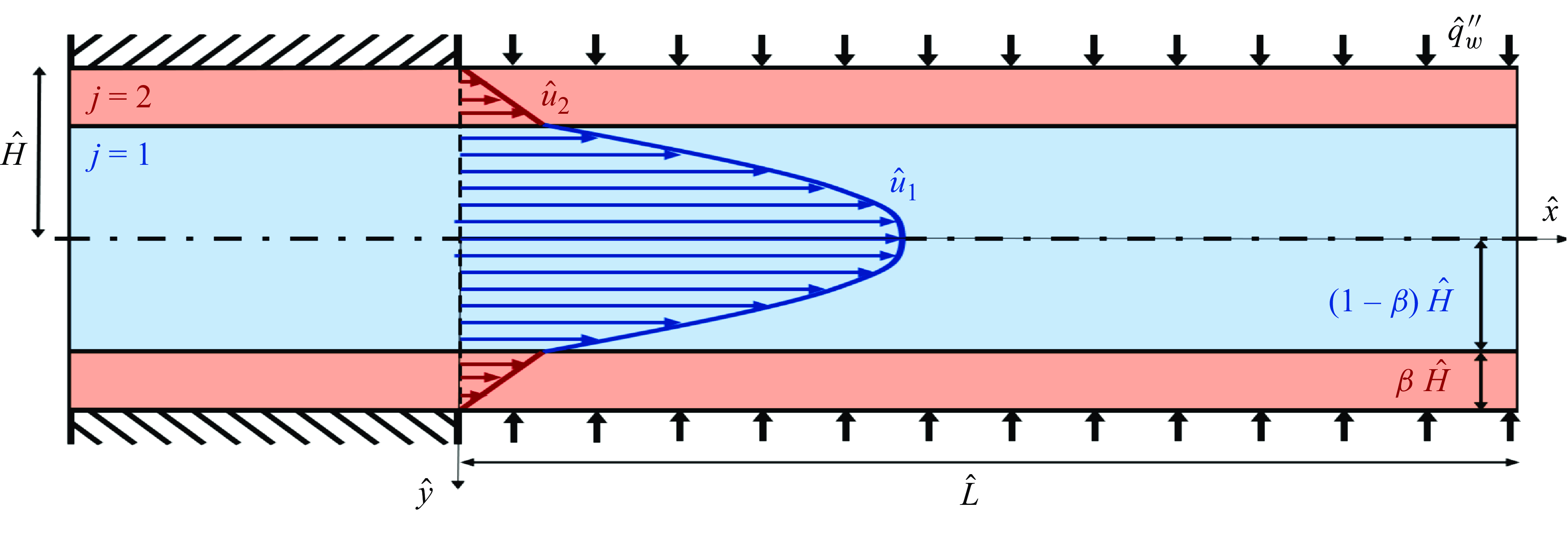
Figure 1. Schematic diagram of the extended Graetz–Brinkman problem for a laminar two-phase core-annular flow in a plane slender channel ( $\hat {H}\ll \hat {L}$
) with a semi-infinite heating section.
$\hat {H}\ll \hat {L}$
) with a semi-infinite heating section.
Starting from transport equations (§ 2.1), we derive a set of coupled evolution equations for the average temperatures as functions of space and time by means of two-scale asymptotic expansions (§ 3). Our analysis (the full derivation is presented in Appendix C) is complemented by a rigorous specification of the theoretical bounds of validity of the model (§ 3.1). In the case of large thermal conductivity contrast between the phases, the system reduces to a single equation (§ 3.2), which admits an analytical solution (§ 4.1), including transient effects. Instead, when the thermal conductivities are of the same order of magnitude, the problem is described by two coupled advection–heat-transfer equations and an analytical solution only exists at the steady-state (§ 4.5). Finally, we derive analytical scaling laws for the asymptotic Nusselt number (§§ 4.2, 4.7) and discuss the thermal coupling between the phases (Brenner Reference Brenner1982; Chu, Sposito & Jury Reference Chu, Sposito and Jury1983; Auriault & Lewandowska Reference Auriault and Lewandowska1994; Moyne & Murad Reference Moyne and Murad2006; Shelukhin, Yeltsov & Paranichev Reference Shelukhin, Yeltsov and Paranichev2011). These results shed light on heat transfer phenomena in the context of multi-phase flows and may serve as a starting step to generalise the heat transfer model to other flow regimes.
2. Problem formulation
We consider an infinitely long and horizontal planar channel with a uniform cross-section of height $2\hat {H}$
, as sketched in figure 1; the hat operator will be used to denote dimensional quantities. Two immiscible Newtonian fluids flow from left to right as a core-annular flow regime driven by a constant pressure gradient: the inner fluid, which is not in contact with the channel wall, will be denoted by subscript ‘1’, while the outer fluid that is in contact with the channel wall will be denoted by subscript ‘2’. The fluid–fluid interface is supposed to be flat, and both velocity profiles are assumed to be fully developed and laminar. The channel is heated by a constant and uniform wall heat flux
$2\hat {H}$
, as sketched in figure 1; the hat operator will be used to denote dimensional quantities. Two immiscible Newtonian fluids flow from left to right as a core-annular flow regime driven by a constant pressure gradient: the inner fluid, which is not in contact with the channel wall, will be denoted by subscript ‘1’, while the outer fluid that is in contact with the channel wall will be denoted by subscript ‘2’. The fluid–fluid interface is supposed to be flat, and both velocity profiles are assumed to be fully developed and laminar. The channel is heated by a constant and uniform wall heat flux $\hat {q}_{w}^{\prime \prime }$
imposed at both plates (
$\hat {q}_{w}^{\prime \prime }$
imposed at both plates ( $\hat {y}=\pm \,\hat {H}$
) over the entire semi-infinite domain (
$\hat {y}=\pm \,\hat {H}$
) over the entire semi-infinite domain ( $\hat {x}\geqslant 0$
). We primarily consider liquid–liquid systems or gas–liquid systems with sufficiently small temperature differences so that the thermal expansion of the gaseous phase can be neglected. The dimensional velocity profile in each fluid domain is derived from the incompressible Navier–Stokes equation for co-current core-annular flows in a planar geometry:
$\hat {x}\geqslant 0$
). We primarily consider liquid–liquid systems or gas–liquid systems with sufficiently small temperature differences so that the thermal expansion of the gaseous phase can be neglected. The dimensional velocity profile in each fluid domain is derived from the incompressible Navier–Stokes equation for co-current core-annular flows in a planar geometry:
 \begin{gather} \hat {u}_{1}\left (\hat {y}\right )=\frac {1}{2{\mu }_{1}}\frac {\mathrm{d}\hat {p}}{\mathrm{d}\hat {x}}\left \{\hat {y}^{2}-\frac {\hat {H}^{2}\left [\mu _{2}-\beta (2-\beta)\left (\mu _{2}-\mu _{1}\right )\right ]}{\mu _{2}}\right \},\quad \frac {\hat {y}}{\hat {H}}\in \left [0;\,1-\beta \right ], \end{gather}
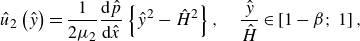 \begin{gather} \hat {u}_{2}\left (\hat {y}\right )=\frac {1}{2{\mu }_{2}}\frac {\mathrm{d}\hat {p}}{\mathrm{d}\hat {x}} \left \{\hat {y}^{2}-\hat {H}^{2}\right \},\quad \frac {\hat {y}}{\hat {H}}\in \left [1-\beta ;\,1\right ], \end{gather}
where ${\textrm {d}\hat {p}}/\textrm {d}{\hat {x}}\lt 0$
is the axial pressure gradient,
${\textrm {d}\hat {p}}/\textrm {d}{\hat {x}}\lt 0$
is the axial pressure gradient, $\mu _{j}$
is the dynamical viscosity of the two fluids,
$\mu _{j}$
is the dynamical viscosity of the two fluids, $j=\{1,\,2\}$
, and
$j=\{1,\,2\}$
, and $\beta$
is the volume fraction of the outer phase (
$\beta$
is the volume fraction of the outer phase ( $0\lt \beta \lt 1$
); the detailed derivation of the velocity profiles is given in Appendix A. Specifically, half the thickness of the inner and the outer phase is equal to
$0\lt \beta \lt 1$
); the detailed derivation of the velocity profiles is given in Appendix A. Specifically, half the thickness of the inner and the outer phase is equal to $ (1-\beta )\hat {H}$
and
$ (1-\beta )\hat {H}$
and $\beta \hat {H}$
, respectively.
$\beta \hat {H}$
, respectively.
We obtain the averaged speed of the inner and outer phase by integrating the velocity profiles (2.1),
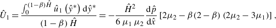 \begin{align} \hat {U}_{1}&=\frac {\int _{0}^{\left (1-\beta \right )\hat {H}}\hat {u}_{1}\left (\hat {y}^{\ast }\right )\mathrm{d}\hat {y}^{\ast }}{\left (1-\beta \right )\hat {H}}= -\frac {\hat {H}^{2}}{6\,\mu _{1}\,\mu _{2}}\frac {\mathrm{d}\hat {p}}{\mathrm{d}\hat {x}}\left [2\mu _{2}-\beta (2-\beta)\left (2\mu _{2}-3\mu _{1}\right ) \right ], \end{align}
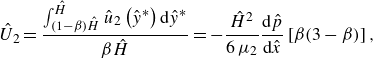 \begin{align} \hat {U}_{2}&=\frac {\int ^{\hat {H}}_{\left (1-\beta \right )\hat {H}}\hat {u}_{2}\left (\hat {y}^{\ast }\right )\mathrm{d}\hat {y}^{\ast }}{\beta \hat {H}}= -\frac {\hat {H}^{2}}{6\,\mu _{2}}\frac {\mathrm{d}\hat {p}}{\mathrm{d}\hat {x}}\left [\beta (3-\beta )\right ], \end{align}
yielding an overall expression for the averaged speed over the entire channel,
 \begin{equation} \hat {U}=\left (1-\beta \right )\hat {U}_{1}+\beta \,\hat {U}_{2}=-\frac {\hat {H}^{2}}{3\,\mu _{1}\,\mu _{2}}\frac {\mathrm{d}\hat {p}}{\mathrm{d}\hat {x}} [\mu _{2}-\beta (\beta ^{2}-3 \beta +3) (\mu _{2}-\mu _{1})]. \end{equation}
2.1. Governing equations for heat transfer
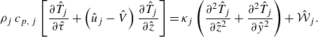
The internal energy balance for each phase written in terms of temperature $\hat {T}_{j} (\hat {x},\,\hat {y},\,\hat {t} )$
is given by
$\hat {T}_{j} (\hat {x},\,\hat {y},\,\hat {t} )$
is given by
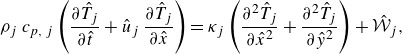 \begin{equation} \rho_{j}\,c_{p,\,j}\left (\frac {\partial \hat {T}_{j}}{\partial \hat {t}}+\hat {u}_{j}\,\frac {\partial \hat {T}_{j}}{\partial \hat {x}}\right )=\kappa _{j}\left (\frac {\partial ^{2} \hat {T}_{j}}{\partial \hat {x}^{2}}+\frac {\partial ^{2} \hat {T}_{j}}{\partial \hat {y}^{2}} \right )+\hat {\mathcal{W}}_{j}, \end{equation}
with $\rho _{j}$
,
$\rho _{j}$
, $c_{p,\,j}$
,
$c_{p,\,j}$
, $\kappa_{j}$
being the density, the isobaric mass heat capacity and the thermal conductivity of each phase, respectively. The term
$\kappa_{j}$
being the density, the isobaric mass heat capacity and the thermal conductivity of each phase, respectively. The term $\hat {\mathcal{W}}_{j}$
represents the rate of viscous dissipation of mechanical energy per unit mass and, for laminar unidirectional and fully developed flows, it reduces to
$\hat {\mathcal{W}}_{j}$
represents the rate of viscous dissipation of mechanical energy per unit mass and, for laminar unidirectional and fully developed flows, it reduces to
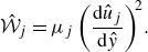 \begin{equation} \hat {\mathcal{W}}_{j}=\mu _{j}\left (\frac {\mathrm{d}\hat {u}_{j}}{\mathrm{d}\hat {y}}\right )^{\!2}\!. \end{equation}
At the channel wall, $\hat {y}=\hat {H}$
, we assume that a uniform heat flux (UWF) is imposed (Shah & London Reference Shah and London1978), leading to
$\hat {y}=\hat {H}$
, we assume that a uniform heat flux (UWF) is imposed (Shah & London Reference Shah and London1978), leading to
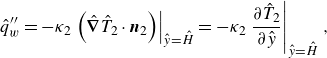 \begin{equation} \hat {q}_{w}^{\prime \prime }=-\kappa _{2}\left .\left (\hat {\boldsymbol{\nabla }}\hat {T}_{2}\cdot \boldsymbol{n}_{2}\right )\right |_{\hat {y}=\hat {H}}= -\kappa _2\left .\frac {\partial \hat {T}_{2}}{\partial \hat {y}}\right |_{\hat {y}=\hat {H}}, \end{equation}
where the unit vector is given by $\boldsymbol{n}_{2}= (0;\,1 )$
. From the practical point of view, an imposed uniform wall heat flux (for
$\boldsymbol{n}_{2}= (0;\,1 )$
. From the practical point of view, an imposed uniform wall heat flux (for $\hat {x}\geqslant 0$
) can be seen as an approximation of many experimental facilities where the channel is wrapped with a heat tape or wire resistance heater – see, for instance, Murphy, Alimohammadi & O’Shaughnessy (Reference Murphy, Alimohammadi and O’Shaughnessy2024). In (2.6), we adopt as convention that the imposed heat flux is positive,
$\hat {x}\geqslant 0$
) can be seen as an approximation of many experimental facilities where the channel is wrapped with a heat tape or wire resistance heater – see, for instance, Murphy, Alimohammadi & O’Shaughnessy (Reference Murphy, Alimohammadi and O’Shaughnessy2024). In (2.6), we adopt as convention that the imposed heat flux is positive, $\hat {q}_{w}^{\prime \prime }\gt 0$
, when it exits the fluid. At the fluid–fluid interface,
$\hat {q}_{w}^{\prime \prime }\gt 0$
, when it exits the fluid. At the fluid–fluid interface, $\hat {y}= (1-\beta )\hat {H}$
, the normal vectors are given by
$\hat {y}= (1-\beta )\hat {H}$
, the normal vectors are given by $\boldsymbol{n}_{1}= (0;\,1 )=-\boldsymbol{n}_{2}$
, and the continuity of temperature and heat flux across the flat interface gives
$\boldsymbol{n}_{1}= (0;\,1 )=-\boldsymbol{n}_{2}$
, and the continuity of temperature and heat flux across the flat interface gives
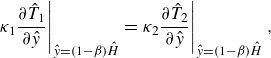 \begin{align} \left .\kappa _{1}\frac {\partial \hat {T}_{1}}{\partial \hat {y}}\right |_{\hat {y}=\left (1-\beta \right )\hat {H}}&= \left .\kappa _{2}\frac {\partial \hat {T}_{2}}{\partial \hat {y}}\right |_{\hat {y}=\left (1-\beta \right )\hat {H}}, \\[-18pt] \nonumber \end{align}
 \begin{align} \left .\hat {T}_{1}\right |_{\hat {y}=\left (1-\beta \right )\hat {H}}&=\left .\hat {T}_{2}\right |_{\hat {y}=\left (1-\beta \right )\hat {H}}. \end{align}
In the duct cross-section at $\hat {y}=0$
, the symmetry of the thermal problem results in
$\hat {y}=0$
, the symmetry of the thermal problem results in
 \begin{equation} \left .\frac {\partial \hat {T}_{1}}{\partial \hat {y}}\right |_{\hat {y}=0}=0. \end{equation}
The problem is closed imposing the initial condition at the channel entry as a uniform temperature distribution at $\hat {t}=0$
and
$\hat {t}=0$
and $\hat {x}=0$
for both phases:
$\hat {x}=0$
for both phases:
 \begin{equation} \hat {T}_{j}\left (0,\,\hat {y},\,0\right )=\hat {T}_{{in},\,j}. \end{equation}
As it will be discussed in § 2.2, we are not focused on describing the early-time evolution of the system and, therefore, the initial condition (2.9) is unimportant for the purposes of our analysis.
Then, we recast the energy balance (2.4), written with respect to an absolute reference frame $ (\hat {x},\,\hat {y} )$
, introducing a new axial coordinate
$ (\hat {x},\,\hat {y} )$
, introducing a new axial coordinate $\hat {z}=\hat {x}-\hat {V}\,\hat {t}$
that advects in the direction of the flow with an arbitrary speed
$\hat {z}=\hat {x}-\hat {V}\,\hat {t}$
that advects in the direction of the flow with an arbitrary speed $\hat {{V}}$
(with
$\hat {{V}}$
(with $\hat {\tau }=\hat {t}$
) yielding
$\hat {\tau }=\hat {t}$
) yielding
 \begin{equation} \rho _{j}\,c_{p,\,j}\left [\frac {\partial \hat {T}_{j}}{\partial \hat {\tau }}+\left (\hat {u}_{j}-\hat {V}\right )\frac {\partial \hat {T}_{j}}{\partial \hat {z}}\right ]=\kappa _{j}\left (\frac {\partial ^{2} \hat {T}_{j}}{\partial \hat {z}^{2}}+\frac {\partial ^{2} \hat {T}_{j}}{\partial \hat {y}^{2}} \right )+\hat {\mathcal{W}}_{j}. \end{equation}
In general, the choice of the reference frame speed $\hat {V}$
is arbitrary (Brady Reference Brady1975), but it affects the definition of the integral variables (e.g. the effective diffusion coefficients). Specifically,
$\hat {V}$
is arbitrary (Brady Reference Brady1975), but it affects the definition of the integral variables (e.g. the effective diffusion coefficients). Specifically, $\hat {V}=0$
corresponds to a description given in the absolute coordinate system; this reference frame will be adopted to compute the bulk temperature and the Nusselt number. Choosing
$\hat {V}=0$
corresponds to a description given in the absolute coordinate system; this reference frame will be adopted to compute the bulk temperature and the Nusselt number. Choosing $\hat {V}=\hat {U}$
identifies the volume-fixed reference frame, i.e. a relative coordinate system moving a speed equal to the mean flow velocity, see (2.3). This reference frame will be used when the focus is on revealing the impact of advection on multiphase heat transfer (i.e. the equivalent of hydrodynamic dispersion in mass transfer problems (Taylor Reference Taylor1953)). In cases where the two phases are thermally decoupled, it is convenient to choose a reference frame attached to the annulus with
$\hat {V}=\hat {U}$
identifies the volume-fixed reference frame, i.e. a relative coordinate system moving a speed equal to the mean flow velocity, see (2.3). This reference frame will be used when the focus is on revealing the impact of advection on multiphase heat transfer (i.e. the equivalent of hydrodynamic dispersion in mass transfer problems (Taylor Reference Taylor1953)). In cases where the two phases are thermally decoupled, it is convenient to choose a reference frame attached to the annulus with $\hat {V}=\hat {U}_{2}$
. A rigorous justification of this argument is provided both in the framework of statistical moments (Aris Reference Aris1956) or perturbation analysis enforcing the Fredholm-type solvability condition (Mauri Reference Mauri1991, Reference Mauri1995, Reference Mauri2015; Mikelić, Devigne & van Duijn Reference Mikelić, Devigne and van Duijn2006). Note that other choices of the reference frame can be made (e.g. molar or mass mean velocity), but their use is limited to multicomponent systems (Hooyman Reference Hooyman1956; Brady Reference Brady1975; Piña Reference Piña1979; Taylor & Krishna Reference Taylor and Krishna1993; Kozlova et al. Reference Kozlova, Mialdun, Ryzhkov, Janzen, Vrabec and Shevtsova2019).
$\hat {V}=\hat {U}_{2}$
. A rigorous justification of this argument is provided both in the framework of statistical moments (Aris Reference Aris1956) or perturbation analysis enforcing the Fredholm-type solvability condition (Mauri Reference Mauri1991, Reference Mauri1995, Reference Mauri2015; Mikelić, Devigne & van Duijn Reference Mikelić, Devigne and van Duijn2006). Note that other choices of the reference frame can be made (e.g. molar or mass mean velocity), but their use is limited to multicomponent systems (Hooyman Reference Hooyman1956; Brady Reference Brady1975; Piña Reference Piña1979; Taylor & Krishna Reference Taylor and Krishna1993; Kozlova et al. Reference Kozlova, Mialdun, Ryzhkov, Janzen, Vrabec and Shevtsova2019).
2.2. Dimensionless formulation
The governing equations introduced in § 2.1 are made dimensionless to facilitate the derivation of an effective description of two-phase flow heat transfer. The relevant scale along the $\hat {y}$
-direction is chosen as the half-distance between the parallel plates
$\hat {y}$
-direction is chosen as the half-distance between the parallel plates $\hat {H}$
, while we denote by
$\hat {H}$
, while we denote by $\hat {L}$
a characteristic macroscopic/observation length scale along the
$\hat {L}$
a characteristic macroscopic/observation length scale along the $\hat {x}$
-axis. We look at systems that can be treated as a shallow geometry,
$\hat {x}$
-axis. We look at systems that can be treated as a shallow geometry, $\hat {L}\gg \hat {H}$
, and, therefore, a small scale parameter indicating the separation between transverse and axial variables arises naturally,
$\hat {L}\gg \hat {H}$
, and, therefore, a small scale parameter indicating the separation between transverse and axial variables arises naturally,
 \begin{equation} \varepsilon =\frac {\hat {H}}{\hat {L}}\ll 1. \end{equation}
The scale separation assumption, $\varepsilon \ll 1$
, is a key requirement to simplify the momentum equations and ensures that the lubrication approximation for the flow holds (see Appendix A).
$\varepsilon \ll 1$
, is a key requirement to simplify the momentum equations and ensures that the lubrication approximation for the flow holds (see Appendix A).
The determination of the relevant time scale is not unique (Mauri Reference Mauri1991; Auriault & Adler Reference Auriault and Adler1995; Mikelić et al. Reference Mikelić, Devigne and van Duijn2006; Battiato & Tartakovsky Reference Battiato and Tartakovsky2011; Bourbatache et al. Reference Bourbatache, Millet and Moyne2020; Picchi & Poesio Reference Picchi and Poesio2022). In fact, advection introduces three advective time scales depending on whether the focus is on a specific phase or the overall system. Assuming that the characteristic scale for the velocity is the overall flow speed $\hat {U}$
given in (2.3), we can define the axial advective time as
$\hat {U}$
given in (2.3), we can define the axial advective time as $\hat {\tau }_{a}=\hat {L}/\hat {U}$
, while using the phase speed,
$\hat {\tau }_{a}=\hat {L}/\hat {U}$
, while using the phase speed, $U_j$
, we can introduce two additional time scales as
$U_j$
, we can introduce two additional time scales as $\hat {\tau }_{a,\,j}=\hat {L}/\hat {U}_{j}$
. Thermal diffusion introduces two additional time scales for each phase: the axial,
$\hat {\tau }_{a,\,j}=\hat {L}/\hat {U}_{j}$
. Thermal diffusion introduces two additional time scales for each phase: the axial, $\hat {\tau }_{\hat {L},\,j}=\hat {L}^2/\alpha _{j}$
, and the transverse,
$\hat {\tau }_{\hat {L},\,j}=\hat {L}^2/\alpha _{j}$
, and the transverse, $\hat {\tau }_{\hat {H},\,1}={(1-\beta )^{2}\hat {H}}^2/\alpha _{1}$
,
$\hat {\tau }_{\hat {H},\,1}={(1-\beta )^{2}\hat {H}}^2/\alpha _{1}$
, $\hat {\tau }_{\hat {H},\,2}={\beta ^{2}\,\hat {H}}^2/\alpha _{2}$
, diffusion times, with
$\hat {\tau }_{\hat {H},\,2}={\beta ^{2}\,\hat {H}}^2/\alpha _{2}$
, diffusion times, with $\alpha _{j}={\kappa _{j}}/{\rho _{j}\,c_{p,\,j}}$
being the thermal diffusivity of the
$\alpha _{j}={\kappa _{j}}/{\rho _{j}\,c_{p,\,j}}$
being the thermal diffusivity of the $j$
th phase. Since we are primarily interested in transport dynamics in a time frame much larger than the transverse diffusion time and close to the advection time, we choose
$j$
th phase. Since we are primarily interested in transport dynamics in a time frame much larger than the transverse diffusion time and close to the advection time, we choose $\hat {\tau }_a$
as the reference scale for the time variable (Mauri Reference Mauri1991; Griffiths et al. Reference Griffiths, Howell and Shipley2013; Mauri Reference Mauri2015; Ling et al. Reference Ling, Tartakovsky and Battiato2016; Liñán et al. Reference Liñán, Rajamanickam, Weiss, A. and Sánchez2020). This choice allows the investigation of heat-transfer regimes characterised by the competition between advection and axial diffusion. In fact, as elucidated by Taylor’s analysis of solute dispersion (Taylor Reference Taylor1953), the advective time scale corresponds to a time window that is intermediate between the times characterising transverse and axial diffusion, i.e.
$\hat {\tau }_a$
as the reference scale for the time variable (Mauri Reference Mauri1991; Griffiths et al. Reference Griffiths, Howell and Shipley2013; Mauri Reference Mauri2015; Ling et al. Reference Ling, Tartakovsky and Battiato2016; Liñán et al. Reference Liñán, Rajamanickam, Weiss, A. and Sánchez2020). This choice allows the investigation of heat-transfer regimes characterised by the competition between advection and axial diffusion. In fact, as elucidated by Taylor’s analysis of solute dispersion (Taylor Reference Taylor1953), the advective time scale corresponds to a time window that is intermediate between the times characterising transverse and axial diffusion, i.e. $\tau _{H,j}\ll \tau _a \ll \tau _{L,j}$
, defining a hierarchy of time scales that can be uniquely determined in terms of the scale parameter
$\tau _{H,j}\ll \tau _a \ll \tau _{L,j}$
, defining a hierarchy of time scales that can be uniquely determined in terms of the scale parameter $\varepsilon$
and the Péclet number of the problem (see § 4.3). This choice of the relevant time window also implies that the model is not capable of describing the early-time relaxation of the system’s initial configuration due to transverse diffusion (known as pre-asymptotic regime) and, therefore, the initial condition given in (2.9) will not be considered. Note that the description of the pre-asymtotic regime (see e.g. Taghizadeh, Valdés-Parada & Wood (Reference Taghizadeh, Valdés-Parada and Wood2020)) is out of the scope of this work.
$\varepsilon$
and the Péclet number of the problem (see § 4.3). This choice of the relevant time window also implies that the model is not capable of describing the early-time relaxation of the system’s initial configuration due to transverse diffusion (known as pre-asymptotic regime) and, therefore, the initial condition given in (2.9) will not be considered. Note that the description of the pre-asymtotic regime (see e.g. Taghizadeh, Valdés-Parada & Wood (Reference Taghizadeh, Valdés-Parada and Wood2020)) is out of the scope of this work.
We can recast the energy balance (2.10) introducing the following dimensionless variables:
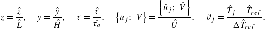 \begin{equation} z=\frac {\hat {z}}{\hat {L}}, \quad y=\frac {\hat {y}}{\hat {H}}, \quad \tau =\frac {\hat {\tau }}{\hat {\tau _a}},\quad \left \{u_{j};\,V\right \}= \frac {\left \{\hat {u}_{j};\,\hat {V}\right \}}{\hat {U}}, \quad \vartheta _{j}=\frac {\hat {T}_{j}-\hat {T}_{{ref}}}{\Delta \hat {T}_{{ref}}}, \end{equation}
where $\hat {T}_{{ref}}$
and
$\hat {T}_{{ref}}$
and $\Delta \hat {T}_{{ref}}$
are arbitrary reference values for the temperature and its variation, respectively. For example, the reference temperature
$\Delta \hat {T}_{{ref}}$
are arbitrary reference values for the temperature and its variation, respectively. For example, the reference temperature $\hat {T}_{{ref}}$
can be chosen as the initial temperature at a given location (
$\hat {T}_{{ref}}$
can be chosen as the initial temperature at a given location ( $\hat {x}=0$
),
$\hat {x}=0$
), $\hat {T}_{{in}}$
, while the reference temperature difference
$\hat {T}_{{in}}$
, while the reference temperature difference $\Delta \hat {T}_{{ref}}$
can be defined based on the condition of uniform heat flux at the wall, as
$\Delta \hat {T}_{{ref}}$
can be defined based on the condition of uniform heat flux at the wall, as $\hat {q}_{w}^{\prime \prime }\,\hat {L}/\kappa _{2}$
(Shah & London Reference Shah and London1978) or
$\hat {q}_{w}^{\prime \prime }\,\hat {L}/\kappa _{2}$
(Shah & London Reference Shah and London1978) or $\hat {q}_{w}^{\prime \prime }\,\hat {L}/(\rho _{2}\,c_{p,\,2}\,\hat {U}\hat {H})$
(Chen et al. Reference Chen, Cotta, Naveira-Cotta and Pontes2022). This procedure yields
$\hat {q}_{w}^{\prime \prime }\,\hat {L}/(\rho _{2}\,c_{p,\,2}\,\hat {U}\hat {H})$
(Chen et al. Reference Chen, Cotta, Naveira-Cotta and Pontes2022). This procedure yields
 \begin{align} \varepsilon \,\mathcal{A}\,{\textit{Pe}}\left [\frac {\partial \vartheta _{1}}{\partial \tau }+\left (u_{1}-V\right )\frac {\partial \vartheta _{1}}{\partial z}\right ] &= \left (\varepsilon ^{2}\,\frac {\partial ^{2} \vartheta _{1}}{\partial z^{2}}+\frac {\partial ^{2} \vartheta _{1}}{\partial y^{2}}\right ) +\frac {m}{\mathcal{K}}\,{Br}\left (\frac {\mathrm{d}{u}_{1}}{\mathrm{d}{y}}\right )^{\!2}\!\!, \!\!\quad\!\! y\in \left [0;\,1-\beta \right ], \end{align}
 \begin{align} \varepsilon \,{\textit{Pe}}\left [\frac {\partial \vartheta _{2}}{\partial \tau }+\left (u_{2}-V\right )\frac {\partial \vartheta _{2}}{\partial z}\right ] &= \left (\varepsilon ^{2}\,\frac {\partial ^{2} \vartheta _{2}}{\partial z^{2}}+\frac {\partial ^{2} \vartheta _{2}}{\partial y^{2}}\right ) +{Br}\left (\frac {\mathrm{d}{u}_{2}}{\mathrm{d}{y}}\right )^{\!2}\!\!, \quad\ \, y\in \left [1-\beta ;\,1\right ], \end{align}
where dimensionless absolute velocity profiles $u_{j} (y )$
are given in Appendix A.1. In the following,
$u_{j} (y )$
are given in Appendix A.1. In the following, $V=0$
corresponds to a description given in the absolute coordinate system,
$V=0$
corresponds to a description given in the absolute coordinate system, $V=1$
identifies the relative coordinate system moving at the mean flow speed, while
$V=1$
identifies the relative coordinate system moving at the mean flow speed, while $V=U_{2}$
identifies the reference frame attached to the annulus. The normalisation introduces the viscosity ratio
$V=U_{2}$
identifies the reference frame attached to the annulus. The normalisation introduces the viscosity ratio $m$
, the thermal conductivity ratio
$m$
, the thermal conductivity ratio $\mathcal{K}$
and the thermal diffusivity ratio
$\mathcal{K}$
and the thermal diffusivity ratio $\mathcal{A}$
:
$\mathcal{A}$
:
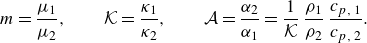 \begin{equation} m=\frac {\mu _{1}}{\mu _{2}}, \qquad \mathcal{K}=\frac {\kappa _{1}}{\kappa _{2}}, \qquad \mathcal{A}=\frac {\alpha _{2}}{\alpha _{1}}=\frac {1}{\mathcal{K}}\,\frac {\rho _{1}}{\rho _{2}}\,\frac {c_{p,\,1}}{c_{p,\,2}}. \end{equation}
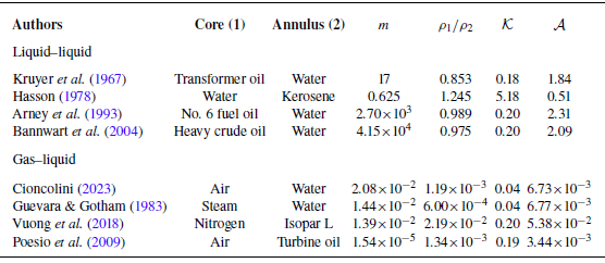
The viscosity ratio accounts for the different viscosity of the flowing phases: when $m\to 0$
, the outer fluid is much more viscous compared with the inner one as typical of the majority of gas–liquid systems (see table 1); we will refer to this limit as the free-surface limit. When
$m\to 0$
, the outer fluid is much more viscous compared with the inner one as typical of the majority of gas–liquid systems (see table 1); we will refer to this limit as the free-surface limit. When $m\to \infty$
, the inner fluid is much more viscous than the outer one and it behaves like a rigid body, see figure 3(a); we will refer to this limit as the rigid-core limit. The product
$m\to \infty$
, the inner fluid is much more viscous than the outer one and it behaves like a rigid body, see figure 3(a); we will refer to this limit as the rigid-core limit. The product $\mathcal{K}\,\mathcal{A}$
can be seen as the thermal capacity ratio: gas–liquid systems are characterised by lower values of
$\mathcal{K}\,\mathcal{A}$
can be seen as the thermal capacity ratio: gas–liquid systems are characterised by lower values of $\mathcal{K}\,\mathcal{A}$
with respect to liquid–liquid systems (see table 1). Note that, although in our model, the physical properties of the two phases appear in the three property ratios given in (2.14), other sets of dimensionless parameters can provide an equivalent description. For example, in Appendix B, we show how the property ratios (2.14) can be recast in terms of the heat-capacity flow rate ratio, commonly used to describe heat-exchanger problems.
$\mathcal{K}\,\mathcal{A}$
with respect to liquid–liquid systems (see table 1). Note that, although in our model, the physical properties of the two phases appear in the three property ratios given in (2.14), other sets of dimensionless parameters can provide an equivalent description. For example, in Appendix B, we show how the property ratios (2.14) can be recast in terms of the heat-capacity flow rate ratio, commonly used to describe heat-exchanger problems.
In (2.13), the Péclet number ${\textit{Pe}}$
and the Brinkman number
${\textit{Pe}}$
and the Brinkman number ${Br}$
for the outer phase are given by
${Br}$
for the outer phase are given by
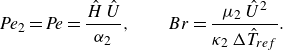 \begin{equation} {\textit{Pe}}_{2} = {\textit{Pe}} = \frac {\hat {H}\,\hat {U}}{\alpha _{2}},\qquad {Br} = \frac {\mu _{2}\,\hat {U}^{2}}{\kappa _{2}\,\Delta \hat {T}_{{ref}}}. \end{equation}
The Péclet number expresses the ratio between advection and axial diffusion. When ${\textit{Pe}}\ll 1$
, diffusion dominates over advection, while for
${\textit{Pe}}\ll 1$
, diffusion dominates over advection, while for ${\textit{Pe}}\gg 1$
, advection plays a major role with respect to diffusion. The Péclet number
${\textit{Pe}}\gg 1$
, advection plays a major role with respect to diffusion. The Péclet number ${\textit{Pe}}_{1}$
of the inner phase is given by the product
${\textit{Pe}}_{1}$
of the inner phase is given by the product ${\textit{Pe}}_{1}=\,\mathcal{A}\,{\textit{Pe}}$
. The Brinkman number can be seen as the competition between the thermal power per unit mass produced by viscous dissipation and the one transferred due to conduction by the outer phase through the channel walls;
${\textit{Pe}}_{1}=\,\mathcal{A}\,{\textit{Pe}}$
. The Brinkman number can be seen as the competition between the thermal power per unit mass produced by viscous dissipation and the one transferred due to conduction by the outer phase through the channel walls; $ {Br}=0$
only in non-dissipative flows.
$ {Br}=0$
only in non-dissipative flows.
The dimensionless boundary conditions at the wall (2.6), at the interface (2.7) and at the channel axis (2.8) read
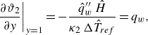 \begin{align} \left .\frac {\partial \vartheta _{2}}{\partial y}\right |_{y=1}&= -\frac {\hat {q}^{\prime \prime }_{w}\,\hat {H}}{\kappa _{2}\,\Delta \hat {T}_{{ref}}}= q_{w}, \end{align}
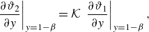 \begin{align} \left .\frac {\partial \vartheta _{2}}{\partial y}\right |_{y=1-\beta }&= \mathcal{K}\,\left .\frac {\partial \vartheta _{1}}{\partial y}\right |_{y=1-\beta }, \end{align}
 \begin{align} \left .{\vartheta _{2}}\right |_{y=1-\beta }&= \left .{\vartheta _{1}}\right |_{y=1-\beta }, \end{align}
 \begin{align} \left .\frac {\partial \vartheta _{1}}{\partial y}\right |_{y=0}&=0. \end{align}
Note that (2.16a
) introduces the dimensionless wall heat flux $q_{w}$
as a further governing dimensionless group.
$q_{w}$
as a further governing dimensionless group.
3. Two-scale asymptotic analysis
The present work aims at obtaining a one-dimensional approximation of the energy equations (2.13) coupled with boundary conditions (2.16). Specifically, we look for one-dimensional advection–diffusion heat-transfer (ADHT) equations accounting for advection, diffusion and heat exchange between the two phases. To do so, we adopt a two-scale asymptotic expansion procedure (Hornung Reference Hornung1997; Boutin, Auriault & Geindreau Reference Boutin, Auriault and Geindreau2010; Bensoussan, Lions & Papanicolaou Reference Bensoussan, Lions and Papanicolaou2011).
-
(i) The starting point is the local description of the dimensionless heat-transfer problem, see (2.13), (2.16), together with the definition of the scale parameter $\varepsilon$
given in (2.11).
$\varepsilon$
given in (2.11). -
(ii) We focus on an asymptotic regime where the temperature profile can be considered almost uniform in the transverse direction (transverse diffusion has smeared out the initial profile) and axial diffusion is part of the game in the spirit of classical Taylor-dispersion theory (Taylor Reference Taylor1953). To this end, we look at axial variations in temperature in between the duct half-height,
$\hat {H}$
, and the duct length,
$\hat {H}/\varepsilon$
, of the order
$1/\sqrt {\varepsilon }$
. Therefore, the longitudinal coordinate
$z$
is re-scaled introducing a stretched spacial variable
$\xi$
(similarly to Griffiths et al. (Reference Griffiths, Howell and Shipley2013); Ling et al. (Reference Ling, Tartakovsky and Battiato2016); Liñán et al. (Reference Liñán, Rajamanickam, Weiss, A. and Sánchez2020)):(3.1)
\begin{equation} \xi =\frac {z}{\sqrt {\varepsilon }}. \end{equation}
-
(iii) The dimensionless groups (2.15), (2.16a ) and the property ratios are evaluated in asymptotic terms expressing their magnitude as integer or half-integer power of the scale parameter
$\varepsilon$
: (3.2a)
\begin{align} \quad \mathcal{K}= K\,\varepsilon ^{k} & \quad \text{with} \quad K=\mathcal{O}\left (1\right )\quad \text{and} \quad k\in \frac {1}{2}\mathbb{Z}, \end{align}
(3.2b)
\begin{align} \mathcal{A}= \varepsilon ^{a}& \quad\text{and} \quad {\textit{Pe}}= \varepsilon ^{-p} \ \ \quad \text{with} \quad a,\,p\in \frac {1}{2}\mathbb{Z}, \end{align}
(3.2c)
\begin{align} \quad {Br}= B\,\varepsilon ^{b} & \quad\text{with} \quad B=\mathcal{O}\left (1\right )\quad \text{and} \quad b\in \frac {1}{2}\mathbb{Z}, \end{align}
(3.2d)
\begin{align} \quad q_{w}= Q\,\varepsilon ^{f} & \quad \text{with} \quad Q=\mathcal{O}\left (1\right )\quad \text{and} \quad f\in \frac {1}{2}\mathbb{Z}. \end{align}
-
(iv) The temperature field
$\vartheta _{j}$
in the energy equations (2.13), (2.16) is written as a half-integer power-series expansion in the scale parameter:(3.3)
\begin{align} \quad \vartheta _{j}\left (\xi, y,\tau ;\,\varepsilon \right ) = \vartheta _{j}^{(0)}\left (\xi, y, \tau \right ) + \sqrt {\varepsilon }\,\vartheta _{j}^{(1)}\left (\xi, y, \tau \right ) + \varepsilon \,\vartheta _{j}^{(2)}\left (\xi, y, \tau \right ) + \mathcal{O}(\varepsilon \sqrt {\varepsilon }),\nonumber\\[-5pt] \end{align}
where
$\vartheta _{j}^{(n)}$
is the
$n$
th-order term in the asymptotic expansion of the temperature field
$\vartheta _{j}$
, with
$j=\{1,\,2\}$
. We follow the classical multiscale approach where the main variables are expanded with respect to space and the axial coordinate is stretched according to (3.1) to properly describe the asymptotic regime (as explained in item (ii)) (Mauri Reference Mauri1991; Griffiths et al. Reference Griffiths, Howell and Shipley2013; Mauri Reference Mauri2015; Ling et al. Reference Ling, Tartakovsky and Battiato2016; Liñán et al. Reference Liñán, Rajamanickam, Weiss, A. and Sánchez2020). An equivalent approach would be to fully expand the independent variables in both time and space (Mauri Reference Mauri1995; Mazzino Reference Mazzino1997; Mauri Reference Mauri2003; Mei & Vernescu Reference Mei and Vernescu2010). -
(v) Then, we collect the terms of the same order obtaining a cascade of boundary-value problems. These are sequentially solved to obtain the effective description of the original problem in terms of the depth-averaged temperatures,
$\langle \vartheta _{j}\rangle (\xi, \,\tau )$
, plus higher-order corrections. To do so, we introduce the cross-sectional averaging operator over each fluid domain(3.4)
\begin{equation} \langle \star _{j}\rangle = \begin{cases} \dfrac {1}{1-\beta }\left (\displaystyle\int _{0}^{1-\beta }\star _{j}\,\mathrm{d}y\right ) & \text{if}\,\, j=1, \\[10pt] \dfrac {1}{\beta }\left (\displaystyle\int _{1-\beta }^{1}\star _{j}\,\mathrm{d}y\right ) & \text{if}\,\, j=2, \end{cases} \end{equation}
consistent with the classical two-scale asymptotic expansion procedure (Hornung Reference Hornung1997; Boutin et al. Reference Boutin, Auriault and Geindreau2010; Bensoussan et al. Reference Bensoussan, Lions and Papanicolaou2011). Other types of mean relevant for heat-transfer problems, such as the mixing-cup (or bulk) temperature, require an a priori knowledge of the temperature field, and, therefore, they will be defined once the model’s solution is determined, see § 3.3.
It will be shown, see Appendix C.2 and (C3a ), that the leading-order term in (3.3) is independent on
$y$
and, therefore,
$\vartheta ^{(0)}_{j} (\xi, \,\tau )\equiv \langle \vartheta ^{(0)}_{j} \rangle (\xi, \,\tau )$
. In this type of approach, the goal is to describe the macroscopic behaviour of the system in terms of the zeroth-order terms
$\vartheta _{j}^{(0)}$
while interpreting higher-order terms in (3.3) as small fluctuations around the zeroth-order values. Thus, without any lack of generality (Mauri Reference Mauri1995), we impose a gauge condition of the type(3.5)
\begin{equation} \left \langle \vartheta ^{(n)}_{j}\left (\xi, \,y,\,\tau \right )\right \rangle \equiv 0 \qquad \text{for}\quad {n}\geqslant 1, \end{equation}
implying that the higher orders do not impact on the averaged temperature
(3.6)
\begin{equation} \left \langle \vartheta _{j}^{(n)}\right \rangle \equiv \vartheta _{j}^{(0)}\,\delta ^{n}_{0}, \end{equation}
where
$\delta _{0}^{n}$
is the Kronecker delta indicator introduced to make the problem derivation more concise(3.7)
\begin{equation} \delta ^{i_{1}}_{i_{2}}= \begin{cases} 0 & \text{if}\,\, i_{1}\neq i_{2}, \\[6pt] 1 & \text{if}\,\, i_{1}= i_{2}. \end{cases} \end{equation}
-
(vi) The effective model is obtained imposing the compatibility condition, (also known as solvability condition or Fredholm alternative) which is the sufficient and necessary condition for the existence of solutions to the successive boundary-value problems. Satisfying the compatibility condition results in setting to zero the average of the expanded governing equation over its domain (Rubinstein & Mauri Reference Rubinstein and Mauri1986; Auriault Reference Auriault2002; Mikelić et al. Reference Mikelić, Devigne and van Duijn2006).


The full derivation following the aforementioned procedure is provided in Appendix C, while the final results are given in upcoming sections, distinguishing between two different scenarios based of the order of magnitude of the thermal conductivity ratio $\mathcal{K}$
, see (3.2a
).
$\mathcal{K}$
, see (3.2a
).
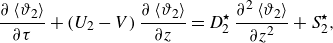
3.1. One-dimensional ADHT equations – coupled regime
The system of ADHT equations, describing the spatial and temporal evolution of the averaged temperatures, is given in (C36), with the coefficients defined in (C37). The corresponding equation in the core is
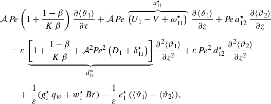 \begin{align} &\mathcal{A}\,{\textit{Pe}}\,{\left (1+\frac {1-\beta }{K\,\beta }\right )}\,\frac {\partial \langle \vartheta _{1}\rangle }{\partial \tau } + \mathcal{A}\,{\textit{Pe}}\, \overbrace {\left (U_{1}-V+\omega _{11}^{\star }\right )}^{a_{11}^{\star }} \,\frac {\partial \langle \vartheta _{1}\rangle }{\partial z} + {\textit{Pe}}\,a_{12}^{\star }\,\frac {\partial \langle \vartheta _{2}\rangle }{\partial z} \nonumber \\[6pt] &\quad =\varepsilon \,\underbrace {\left [1+\frac {1-\beta }{K\,\beta }+\mathcal{A}^{2}{\textit{Pe}}^{2}\left (D_{1}+\delta _{11}^{\star }\right )\right ]}_{d_{11}^{\ast }} \frac {\partial ^{2}\langle \vartheta _{1}\rangle }{\partial z^{2}} + \varepsilon \,{\textit{Pe}}^{2}\,d_{12}^{\star }\,\frac {\partial ^{2}\langle \vartheta _{2}\rangle }{\partial z^{2}} \nonumber \\[4pt] & \qquad +\, \frac {1}{\varepsilon }\big ({g_{1}^{\star }}\,q_{w} + {w_{1}^{\star }}\,{Br}\big ) - \frac {1}{\varepsilon }\,e_{1}^{\star }\,\big (\langle \vartheta _{1}\rangle -\langle \vartheta _{2}\rangle \big ), \end{align}
while for the annulus, we get
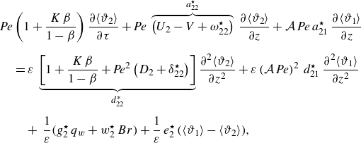 \begin{align} &{\textit{Pe}}\,{\left (1+\frac {K\,\beta }{1-\beta }\right )}\,\frac {\partial \langle \vartheta _{2}\rangle }{\partial \tau } + {\textit{Pe}}\, \overbrace {\left (U_{2}-V+\omega _{22}^{\star }\right )}^{a_{22}^{\star }} \,\frac {\partial \langle \vartheta _{2}\rangle }{\partial z} + \mathcal{A}\,{\textit{Pe}}\,a_{21}^{\star }\,\frac {\partial \langle \vartheta _{1}\rangle }{\partial z} \nonumber \\[6pt] &\quad =\varepsilon \,\underbrace {\left [1+\frac {K\,\beta }{1-\beta }+{\textit{Pe}}^{2}\left (D_{2}+\delta _{22}^{\star }\right )\right ]}_{d_{22}^{\ast }} \frac {\partial ^{2}\langle \vartheta _{2}\rangle }{\partial z^{2}} + \varepsilon \left (\mathcal{A}\,{\textit{Pe}}\right )^{2}\,d_{21}^{\star }\, \frac {\partial ^{2}\langle \vartheta _{1}\rangle }{\partial z^{2}} \nonumber \\[4pt] &\qquad +\, \frac {1}{\varepsilon }\big ({g_{2}^{\star }}\,q_{w} + {w_{2}^{\star }}\,{Br}\big ) + \frac {1}{\varepsilon }\,e_{2}^{\star }\,\big (\langle \vartheta _{1}\rangle -\langle \vartheta _{2}\rangle \big ), \end{align}
with $a_{jj}^{\star }(U_j,\,V,\,\beta, \,m,\,K)$
and
$a_{jj}^{\star }(U_j,\,V,\,\beta, \,m,\,K)$
and $d_{jj}^{\star }(V,\,\beta, \,m,\,K,\,{\textit{Pe}})$
being the effective coefficients for advection and diffusion of the inner (
$d_{jj}^{\star }(V,\,\beta, \,m,\,K,\,{\textit{Pe}})$
being the effective coefficients for advection and diffusion of the inner ( $j=1$
) and the outer phase (
$j=1$
) and the outer phase ( $j=2$
). Those coefficients are a function of the speed of the reference frame,
$j=2$
). Those coefficients are a function of the speed of the reference frame, $V$
, the phase speeds
$V$
, the phase speeds $U_{j}$
, the volume fraction
$U_{j}$
, the volume fraction $\beta$
, the viscosity ratio
$\beta$
, the viscosity ratio $m$
, and the conductivity ratio
$m$
, and the conductivity ratio $\mathcal{K}$
– their full expressions are given in Appendix C.6. The ADHT equations (3.8), (3.9) are coupled through diverse physical mechanisms, namely advection and diffusion of the other phase via the coefficients
$\mathcal{K}$
– their full expressions are given in Appendix C.6. The ADHT equations (3.8), (3.9) are coupled through diverse physical mechanisms, namely advection and diffusion of the other phase via the coefficients $a_{12}^{\star }(\beta, \,m,\,K)$
and
$a_{12}^{\star }(\beta, \,m,\,K)$
and $a_{21}^{\star }(\beta, \,m,\,K)$
, and
$a_{21}^{\star }(\beta, \,m,\,K)$
, and $d_{12}^{\star }(V,\,\beta, \,m,\,K)$
and
$d_{12}^{\star }(V,\,\beta, \,m,\,K)$
and $d_{21}^{\star }(V,\,\beta, \,m,\,K)$
, respectively; heat exchange between the phases through storage terms (
$d_{21}^{\star }(V,\,\beta, \,m,\,K)$
, respectively; heat exchange between the phases through storage terms ( $\propto \pm (\left \langle \vartheta _{1}\right \rangle -\left \langle \vartheta _{2}\right \rangle )$
) and source terms proportional to
$\propto \pm (\left \langle \vartheta _{1}\right \rangle -\left \langle \vartheta _{2}\right \rangle )$
) and source terms proportional to $q_w$
. All these mechanisms will be discussed in detail in § 4.5.
$q_w$
. All these mechanisms will be discussed in detail in § 4.5.
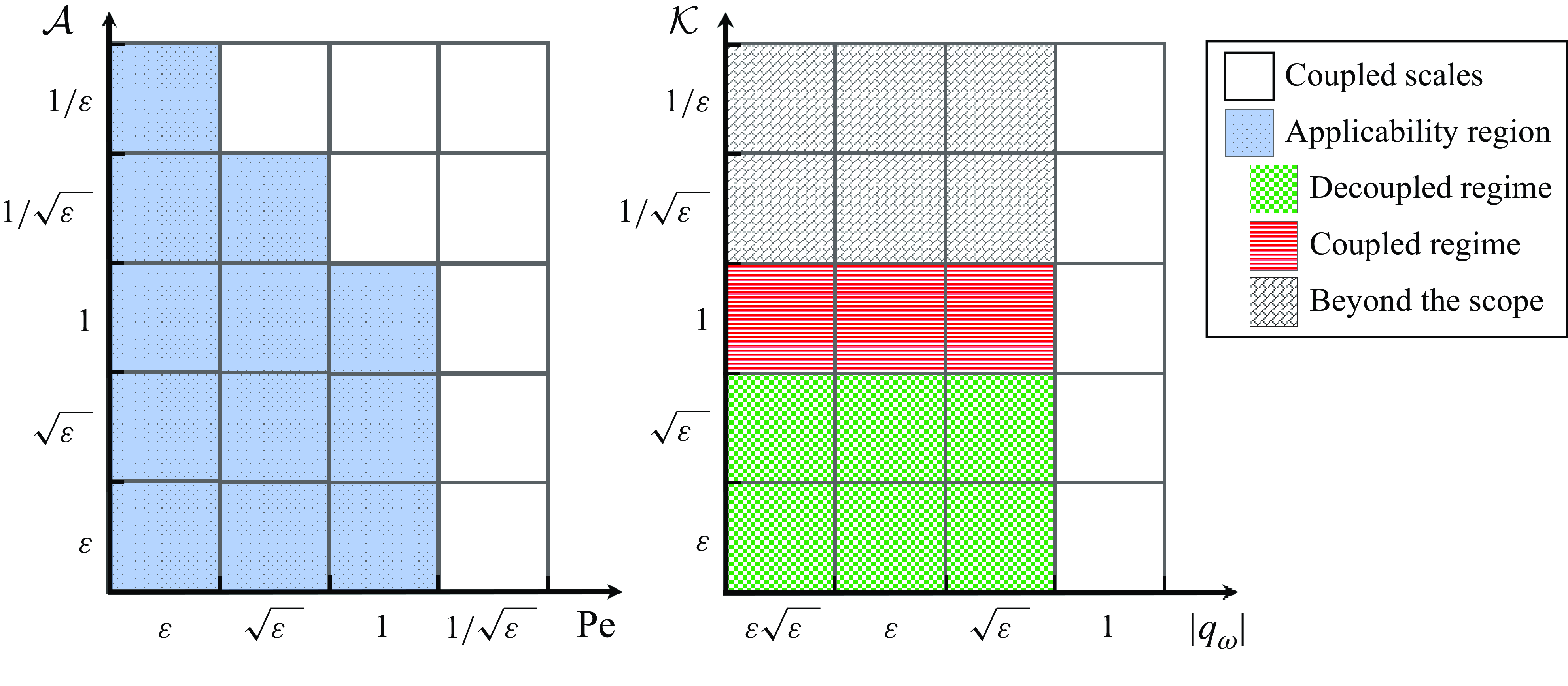
Figure 2. Parameter space of transport regimes in the $({\textit{Pe}},\,\mathcal{A})$
(left) and in the
$({\textit{Pe}},\,\mathcal{A})$
(left) and in the $(q_{w},\,\mathcal{K})$
(right) planes. Coloured areas of the maps correspond to regimes where the effective heat-transfer equation for the averaged temperatures can be formally written by means of two-scale expansion.
$(q_{w},\,\mathcal{K})$
(right) planes. Coloured areas of the maps correspond to regimes where the effective heat-transfer equation for the averaged temperatures can be formally written by means of two-scale expansion.
The ADHT equations (3.8), (3.9) hold only in a specific range of the dimensionless groups (2.14), (2.15), (2.16a ) to guarantee that the two scales can be decoupled. Such requirements are known as the applicability region and are sufficient (but not necessary) conditions for the effective model to be representative of the spatially averaged processes within the error bounds prescribed by the asymptotics. In our case, the upscaled equations hold only when:
-
(i)
$\varepsilon \ll 1$
; -
(ii)
${\textit{Pe}}\ll 1/{\sqrt {\varepsilon }}$
; -
(iii)
$\mathcal{A}\,{\textit{Pe}}\ll 1/{\sqrt {\varepsilon }}$
; -
(iv)
$\left |q_{w}\right |\ll 1$
; -
(v)
${Br}\ll 1$
.


Condition (a) ensures that the spatial scale separation exists. Conditions (b) and (c) provide the upper bounds to the Péclet number of each phase, ensuring that advection does not prevail over diffusion. Condition (d) restricts the rate at which heat is transferred by the external energy source to/from the channel. Finally, condition (e) concerns the Brinkman number, guaranteeing that the impact of viscous shear heating is low enough not to conflict with the other transport phenomena.
The applicability region given by conditions (a)–(e) has been determined from the asymptotic solution developed in Appendix C selecting the order of the dimensionless parameters in such a way that they enter the problem at the highest order compatible with the separation of scales. In other words, the set of exponents $p$
,
$p$
, $a$
,
$a$
, $k$
,
$k$
, $b$
and
$b$
and $f$
has been selected accordingly so that a given term enters into the corresponding order of magnitude depending on the transport regime. Those constraints are sufficient conditions which ensure a rigorous thermal decoupling between the transverse and the axial scales. If such constraints are not met, the idea of cross-sectional averaging (3.4) lacks significance and the accuracy of the upscaled model cannot be guaranteed (Boso & Battiato Reference Boso and Battiato2013). Note that there exists strategies to relax the applicability conditions, for example, using iterative hybrid numerical methods (see Battiato et al. (Reference Battiato, Tartakovsky, Tartakovsky and Scheibe2011)).
$f$
has been selected accordingly so that a given term enters into the corresponding order of magnitude depending on the transport regime. Those constraints are sufficient conditions which ensure a rigorous thermal decoupling between the transverse and the axial scales. If such constraints are not met, the idea of cross-sectional averaging (3.4) lacks significance and the accuracy of the upscaled model cannot be guaranteed (Boso & Battiato Reference Boso and Battiato2013). Note that there exists strategies to relax the applicability conditions, for example, using iterative hybrid numerical methods (see Battiato et al. (Reference Battiato, Tartakovsky, Tartakovsky and Scheibe2011)).
Figure 2 shows the graphical representation of the conditions (b)–(d). Specifically, we can identify three main regimes based of the order of magnitude of the conductivity ratio $\mathcal{K}$
. When
$\mathcal{K}$
. When $\mathcal{K}=\mathcal{O}(1)$
, the thermal conductivities are of the same order of magnitude and the problem is described by two coupled ADHT equations (3.8), (3.9); this will be referred to as the coupled regime and it is typical of liquid–liquid systems (see table 1). Instead, when the thermal conductivity of the inner phase is small with respect to that of the outer one (
$\mathcal{K}=\mathcal{O}(1)$
, the thermal conductivities are of the same order of magnitude and the problem is described by two coupled ADHT equations (3.8), (3.9); this will be referred to as the coupled regime and it is typical of liquid–liquid systems (see table 1). Instead, when the thermal conductivity of the inner phase is small with respect to that of the outer one ( $\mathcal{K}\leqslant \mathcal{O}(\sqrt {\varepsilon }$
)), the thermal interaction between the phases is negligible and the problem is described by a single ADHT equation for the outer phase, see § 3.2; this will be referred to as the decoupled regime, typical of gas–liquid systems and a few liquid–liquid systems, see table 1. There exists a third regime for
$\mathcal{K}\leqslant \mathcal{O}(\sqrt {\varepsilon }$
)), the thermal interaction between the phases is negligible and the problem is described by a single ADHT equation for the outer phase, see § 3.2; this will be referred to as the decoupled regime, typical of gas–liquid systems and a few liquid–liquid systems, see table 1. There exists a third regime for $\mathcal{K}\geqslant \mathcal{O}(1/\sqrt {\varepsilon })$
that leads to a single equation for the core averaged temperature. In this work, the latest regime will not be considered, since we are mainly interested in two-phase forced-convection configurations where the inner phase is less conductive with respect to the outer phase.
$\mathcal{K}\geqslant \mathcal{O}(1/\sqrt {\varepsilon })$
that leads to a single equation for the core averaged temperature. In this work, the latest regime will not be considered, since we are mainly interested in two-phase forced-convection configurations where the inner phase is less conductive with respect to the outer phase.
Table 1. Physical properties of liquid–liquid and gas–liquid core-annular systems taken from the literature. The property ratios $m$
,
$m$
, $\mathcal{K}$
,
$\mathcal{K}$
, $\mathcal{A}$
denote the viscosity, thermal conductivity and thermal diffusivity ratios, respectively, as defined in (2.14).
$\mathcal{A}$
denote the viscosity, thermal conductivity and thermal diffusivity ratios, respectively, as defined in (2.14).
3.2. Decoupled regime
When the thermal conductivity of the outer phase is greater than that of the inner phase, $\mathcal{K}\leqslant \mathcal{O}(\sqrt {\varepsilon }$
), the thermal interaction is negligible and the fluid–fluid interface can be considered adiabatic (see the derivation in Appendix C.5.1). Thus, in the moving reference frame
$\mathcal{K}\leqslant \mathcal{O}(\sqrt {\varepsilon }$
), the thermal interaction is negligible and the fluid–fluid interface can be considered adiabatic (see the derivation in Appendix C.5.1). Thus, in the moving reference frame $ (z,\,\tau )$
, (3.8), (3.9) reduce to a single ADHT for the averaged temperature of the outer phase
$ (z,\,\tau )$
, (3.8), (3.9) reduce to a single ADHT for the averaged temperature of the outer phase $\left \langle \vartheta _{2}\right \rangle$
:
$\left \langle \vartheta _{2}\right \rangle$
:
 \begin{equation} \frac {\partial \left \langle \vartheta _{2}\right \rangle }{\partial \tau } + \left (U_{2}-V\right )\frac {\partial \left \langle \vartheta _{2}\right \rangle }{\partial z} = D_{2}^{\star }\, \frac {\partial ^{2} \left \langle \vartheta _{2}\right \rangle }{\partial z^{2}} + S_{2}^{\star }, \end{equation}
where
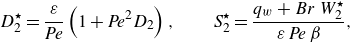 \begin{equation} D_{2}^{\star }= \frac {\varepsilon }{{\textit{Pe}}}\left (1+{\textit{Pe}}^{2}D_{2}\right ), \qquad S_{2}^{\star }= \frac {q_{w}+{Br}\,W_{2}^{\star }}{\varepsilon \,{\textit{Pe}}\,\beta }, \end{equation}
are the effective diffusion coefficient and the effective source term, respectively, whose analytical expressions are given in Appendix C.6. The effective coefficients in (3.10) incorporate the impact of the non-uniformity of the velocity profile (2.1b
) and thermal boundary conditions at the channel axis (2.8) and at the wall (2.6). Specifically, the shear flow spreads the temperature inhomogeneity along the axial direction, affecting axial heat diffusion at sufficiently large Péclet numbers via the coefficient $D_2^\star (V,\,\beta, \,m,\,{\textit{Pe}})$
. The effective sink/source term
$D_2^\star (V,\,\beta, \,m,\,{\textit{Pe}})$
. The effective sink/source term $S^{\star }_{2}$
consists of two distinct contributions:
$S^{\star }_{2}$
consists of two distinct contributions: $q_{w}$
is the heat flux imposed at the wall, while
$q_{w}$
is the heat flux imposed at the wall, while $W_{2}^{\star }$
embeds the effect of viscous dissipation. The trends of the effective coefficients and the analytical solution of the thermal problem in the decoupled regime will be discussed in § 4.1.
$W_{2}^{\star }$
embeds the effect of viscous dissipation. The trends of the effective coefficients and the analytical solution of the thermal problem in the decoupled regime will be discussed in § 4.1.
3.3. Determination of the convective heat-transfer coefficient
The local convective heat-transfer coefficient $h$
is defined via Newton’s law of cooling as the ratio between the thermal power per unit area entering the system and the difference in temperature between the solid surface and a representative temperature for the fluid
$h$
is defined via Newton’s law of cooling as the ratio between the thermal power per unit area entering the system and the difference in temperature between the solid surface and a representative temperature for the fluid $\hat {T}_{b}$
(Incropera Reference Incropera2007):
$\hat {T}_{b}$
(Incropera Reference Incropera2007):
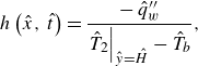 \begin{equation} h\left (\hat {x},\,\hat {t}\right )=\frac {-\,\hat {q}_{w}^{\prime \prime }}{\left .\hat {T}_{2}\right |_{\hat {y}=\hat {H}}-\hat {T}_{b}}, \end{equation}
where $\hat {T}_{b}$
is the bulk temperature; the estimation of
$\hat {T}_{b}$
is the bulk temperature; the estimation of $h$
is provided in the absolute reference frame (
$h$
is provided in the absolute reference frame ( $V=0$
). The bulk (or mixing-cup or flow average) temperature is the temperature reached when a certain amount of fluid reaches the equilibrium without heat loss to the surroundings (Tamir & Taitel Reference Tamir and Taitel1972). It is defined as an enthalpy-weighted average of the phase temperature and for the core-annular flow configuration in figure 1, reads (Su Reference Su2006; Chalhub et al. Reference Chalhub, Corrêa and Teixeira2022)
$V=0$
). The bulk (or mixing-cup or flow average) temperature is the temperature reached when a certain amount of fluid reaches the equilibrium without heat loss to the surroundings (Tamir & Taitel Reference Tamir and Taitel1972). It is defined as an enthalpy-weighted average of the phase temperature and for the core-annular flow configuration in figure 1, reads (Su Reference Su2006; Chalhub et al. Reference Chalhub, Corrêa and Teixeira2022)
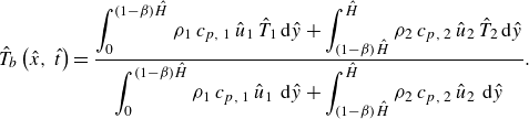 \begin{equation} \hat {T}_{b}\left (\hat {x},\,\hat {t}\right )=\frac {\displaystyle \int _{0}^{\left (1-\beta \right )\hat {H}} \def\lumina\hspace {-0.3cm} \rho _{1}\,c_{p,\,1}\,\hat {u}_{1} \, \hat {T}_{1} \, \mathrm{d}\hat {y}+ \displaystyle \int _{\left (1-\beta \right )\hat {H}}^{\hat {H}} \rho _{2}\,c_{p,\,2}\,\hat {u}_{2} \, \hat {T}_{2} \, \mathrm{d}\hat {y}} {\displaystyle \int _{0}^{\left (1-\beta \right )\hat {H}} \def\lumina\hspace {-0.3cm} \rho _{1}\,c_{p,\,1}\,\hat {u}_{1} \, \, \mathrm{d}\hat {y}+ \displaystyle \int _{\left (1-\beta \right )\hat {H}}^{\hat {H}} \rho _{2}\,c_{p,\,2}\,\hat {u}_{2} \, \, \mathrm{d}\hat {y}}. \end{equation}
Equation (3.12) is made dimensionless using the same scales defined in § 2.2, which gives
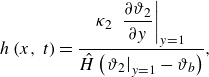 \begin{equation} h\left (x,\,t\right )= \frac {\kappa _{2}\,\left .\dfrac {\partial \vartheta _{2}}{\partial y}\right |_{y=1}}{\hat {H}\left (\left .\vartheta _{2}\right |_{y=1}-\vartheta _{b}\right )}, \end{equation}
where the dimensionless bulk temperature $\vartheta _{b}$
is given combining (3.13) with (2.12), (3.4),
$\vartheta _{b}$
is given combining (3.13) with (2.12), (3.4),
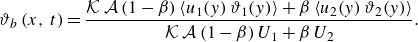 \begin{equation} \vartheta _{b}\left (x,\,t\right )=\frac {\mathcal{K}\,\mathcal{A}\left (1-\beta \right )\big \langle u_{1}(y)\,\vartheta _{1}(y)\big \rangle +\beta \,\big \langle u_{2}(y)\,\vartheta _{2}(y)\big \rangle }{\mathcal{K}\,\mathcal{A}\left (1-\beta \right )U_{1}+\beta \,U_{2}}. \end{equation}
Interestingly, the dimensionless group $\mathcal{K}\,\mathcal{A}$
in (3.15) is the volumetric heat capacity ratio: when
$\mathcal{K}\,\mathcal{A}$
in (3.15) is the volumetric heat capacity ratio: when $\mathcal{K}\,\mathcal{A}\ll 1$
, the bulk temperature simplifies significantly and does not depend anymore on the core properties (this is true for the decoupled regime in § 4.2). Since the averaged temperature
$\mathcal{K}\,\mathcal{A}\ll 1$
, the bulk temperature simplifies significantly and does not depend anymore on the core properties (this is true for the decoupled regime in § 4.2). Since the averaged temperature $\left \langle \vartheta _{2}\right \rangle$
is independent of
$\left \langle \vartheta _{2}\right \rangle$
is independent of $y$
, the temperature (and its derivative) at the wall is calculated considering the power-series truncated to the first order as
$y$
, the temperature (and its derivative) at the wall is calculated considering the power-series truncated to the first order as
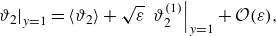 \begin{align} \left .\vartheta _{2}\right |_{y=1}&=\left \langle \vartheta _{2}\right \rangle + \sqrt {\varepsilon }\,\left .\vartheta _{2}^{(1)}\right |_{y=1}+\mathcal{O}(\varepsilon ), \end{align}
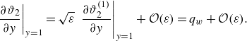 \begin{align} \left .\frac {\partial \vartheta _{2}}{\partial y}\right |_{y=1}&= \sqrt {\varepsilon }\,\left .\frac {\partial \vartheta _{2}^{(1)}}{\partial y}\right |_{y=1} +\mathcal{O}(\varepsilon )=q_{w}+\mathcal{O}(\varepsilon ). \end{align}
In problems of internal forced convection, the heat transfer coefficient is made dimensionless defining the local Nusselt number computed at the wall (Incropera Reference Incropera2007)
 \begin{equation} {\textit{Nu}}\left (x,\,t\right )=\frac {h\,\mathcal{L}}{\kappa _{2}}, \end{equation}
where $\mathcal{L}$
is a characteristic length, typically the hydraulic diameter
$\mathcal{L}$
is a characteristic length, typically the hydraulic diameter $d_{\text{eq}}$
. For the planar configuration depicted in figure 1, the hydraulic diameter can be computed by considering a rectangular slit of width
$d_{\text{eq}}$
. For the planar configuration depicted in figure 1, the hydraulic diameter can be computed by considering a rectangular slit of width $\hat {w}$
and height
$\hat {w}$
and height $2\hat {H}$
, and taking the limit for
$2\hat {H}$
, and taking the limit for $\hat {w}\gg 2\hat {H}$
(see, for instance, Merritt Reference Merritt1991),
$\hat {w}\gg 2\hat {H}$
(see, for instance, Merritt Reference Merritt1991),
 \begin{equation} { d}_{{eq}}=\lim _{\hat {w}\to {\infty }}\frac {8\,\hat {H}\,\hat {w}}{2\left (\hat {w}+2\,\hat {H}\right )}=4\,\hat {H}. \end{equation}
Ultimately, the Nusselt number (3.17) can be expressed as
 \begin{equation} {\textit{Nu}}\left (x,\,t\right )=\dfrac {4\,\left .\dfrac {\partial \vartheta _{2}}{\partial y}\right |_{y=1}}{\left .\vartheta _{2}\right |_{y=1}-\vartheta _{b}}, \end{equation}
in view of (3.18) and (3.14). In the following, when the flow is thermally fully developed, we will refer to as the asymptotic (or limiting) Nusselt number ${\textit{Nu}}^{\infty }$
(Shah & London Reference Shah and London1978).
${\textit{Nu}}^{\infty }$
(Shah & London Reference Shah and London1978).
Finally, for the sake of comparison with the literature, we recast the Brinkman number defined in (2.15b ) (Brinkman Reference Brinkman1951; Bird, Stewart & Lightfoot Reference Bird, Stewart and Lightfoot1960; Boucher & Alves Reference Boucher and Alves1963; Shah & London Reference Shah and London1978) into
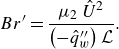 \begin{equation} {Br}^{\prime }=\frac {\mu _{2}\,\hat {U}^{2}}{\left (-\hat {q}_{w}^{\prime \prime }\right )\mathcal{L}}. \end{equation}
In this work, the Brinkman numbers ${Br}$
and
${Br}$
and ${Br}^{\prime }$
are linked to each other by the following relation:
${Br}^{\prime }$
are linked to each other by the following relation:
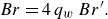 \begin{equation} {Br}=4\,q_{w}\,{Br}^{\prime }. \end{equation}
4. Results and discussion
In this section, we will discuss the heat-transfer model illustrating the main physical mechanisms and deriving a closed-form expression for the Nusselt number for laminar core-annular flows, distinguishing between the decoupled and the coupled regime.
4.1. Heat-transfer mechanisms and temperature field in the decoupled regime
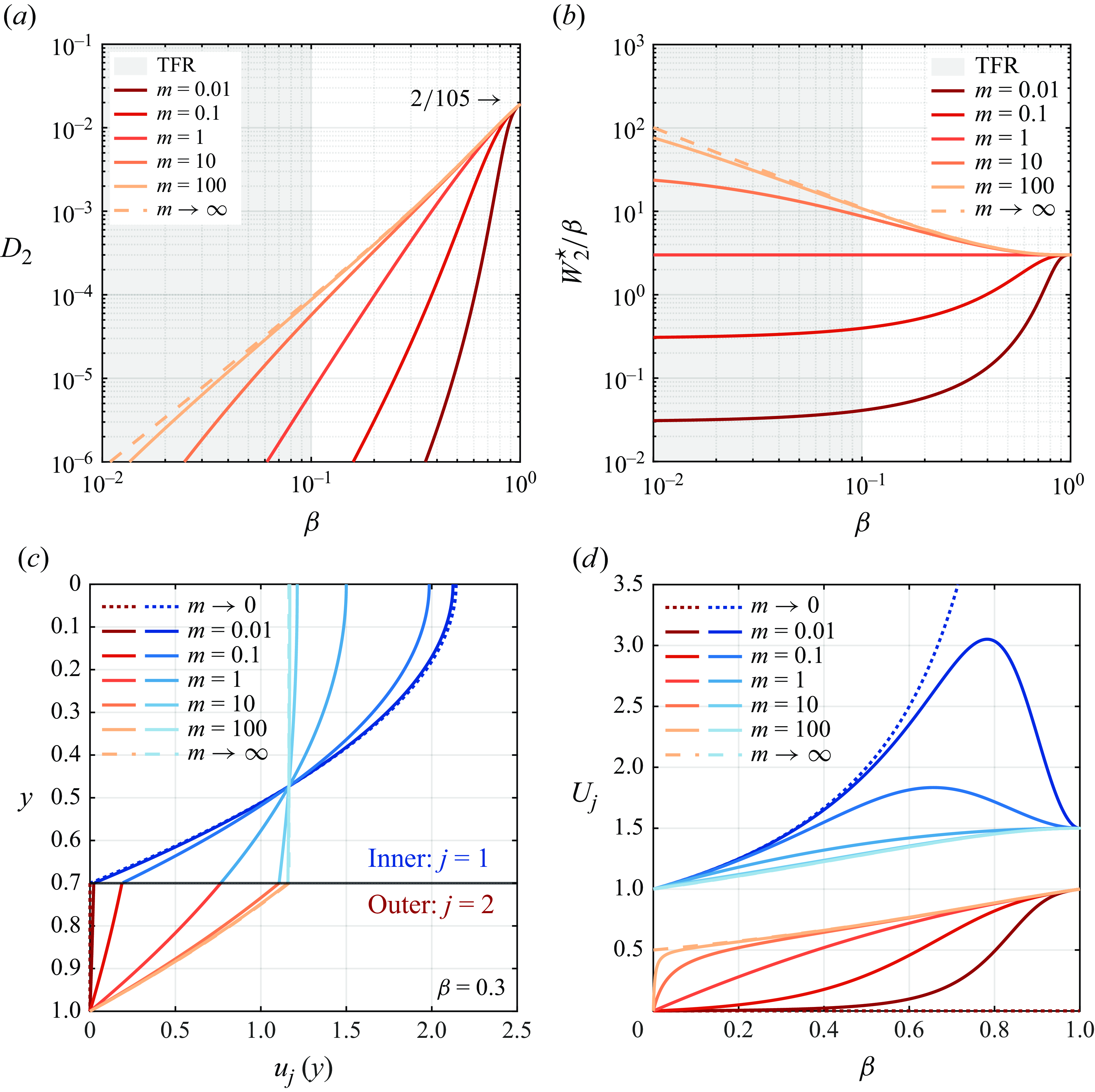
Figure 3. Effect of the viscosity ratio $m$
on (a)
$m$
on (a) $D_{2}$
(in the relative reference frame moving at the mean speed of the annulus,
$D_{2}$
(in the relative reference frame moving at the mean speed of the annulus, $V=U_{2}$
) and (b) the source term related to viscous dissipation
$V=U_{2}$
) and (b) the source term related to viscous dissipation $W_{2}^{\star }/\beta$
, as functions of the volume fraction of the outer phase
$W_{2}^{\star }/\beta$
, as functions of the volume fraction of the outer phase $\beta$
. The thin film region (TFR) is highlighted by the grey area. For both the inner (
$\beta$
. The thin film region (TFR) is highlighted by the grey area. For both the inner ( $j=1$
) and the outer (
$j=1$
) and the outer ( $j=2$
) phase: (c) dimensionless velocity profiles
$j=2$
) phase: (c) dimensionless velocity profiles $u_{j}(y)$
for different values of the viscosity ratio
$u_{j}(y)$
for different values of the viscosity ratio $m$
and a fixed volume fraction
$m$
and a fixed volume fraction $\beta =0.3$
; (d) average speed
$\beta =0.3$
; (d) average speed $U_{j}$
as a function of
$U_{j}$
as a function of $\beta$
and for different values of
$\beta$
and for different values of $m$
.
$m$
.
As described in § 3.2, the decoupled model (3.10) applies to cases where the thermal conductivity of the outer phase is much bigger compared with that of the inner phase, $\mathcal{K}\leqslant \mathcal{O}(\sqrt {\varepsilon })$
. This implies that the inner and the outer phases are thermally decoupled and the model reduces to a ‘one-side’ approach. Such a scenario is typical of the majority of applications, including gas–liquid and liquid–liquid systems (see table 1).
$\mathcal{K}\leqslant \mathcal{O}(\sqrt {\varepsilon })$
. This implies that the inner and the outer phases are thermally decoupled and the model reduces to a ‘one-side’ approach. Such a scenario is typical of the majority of applications, including gas–liquid and liquid–liquid systems (see table 1).
By inspection of (3.10), we see that the temperature evolves in time and space due to three different mechanisms: advection equal to the average speed of the outer phase $U_2$
, effective thermal diffusion through the coefficient
$U_2$
, effective thermal diffusion through the coefficient $D_2^\star$
, and a constant source term
$D_2^\star$
, and a constant source term $S_2^\star$
due to the imposed heat flux at the channel wall and viscous dissipation. Specifically,
$S_2^\star$
due to the imposed heat flux at the channel wall and viscous dissipation. Specifically, $D_2^\star$
has the typical structure of the Aris–Taylor dispersion coefficient (it scales with the square of the Péclet number), being the sum of heat diffusivity, equal to the unity, and axial shear-induced diffusion,
$D_2^\star$
has the typical structure of the Aris–Taylor dispersion coefficient (it scales with the square of the Péclet number), being the sum of heat diffusivity, equal to the unity, and axial shear-induced diffusion, $D_{2}(V,\,\beta, \,m)$
whose expression is given in (C40b
). The latter is an apparent diffusion mechanism for the averaged temperature and has its physical origin in the non-uniformity of the velocity in the outer phase: from the physical point of view, local advection enhances/reduces the axial diffusion in terms of the leading-order variables.
$D_{2}(V,\,\beta, \,m)$
whose expression is given in (C40b
). The latter is an apparent diffusion mechanism for the averaged temperature and has its physical origin in the non-uniformity of the velocity in the outer phase: from the physical point of view, local advection enhances/reduces the axial diffusion in terms of the leading-order variables.
Figure 3(a) shows the evolution of $D_2$
in a coordinate system moving at the mean speed of the outer phase,
$D_2$
in a coordinate system moving at the mean speed of the outer phase, $V=U_{2}$
, according to Aris (Aris Reference Aris1959). In fact, in the decoupled model, thermal dispersion is exclusively driven by the annulus. The presence of the other phase, which acts as a thermal insulator, reduces the effective heat-diffusion compared with the single-phase scenario where
$V=U_{2}$
, according to Aris (Aris Reference Aris1959). In fact, in the decoupled model, thermal dispersion is exclusively driven by the annulus. The presence of the other phase, which acts as a thermal insulator, reduces the effective heat-diffusion compared with the single-phase scenario where $D_2=2/105$
; such a limit is reached only when the core vanishes, i.e. for
$D_2=2/105$
; such a limit is reached only when the core vanishes, i.e. for $\beta \to 1$
. The maximal shear-induced diffusion is obtained in the rigid core limit (
$\beta \to 1$
. The maximal shear-induced diffusion is obtained in the rigid core limit ( $m\to \infty$
), where the velocity profile of the annulus is almost linear (see figure 3
a), maximising the spread of temperature in the axial direction. In the free surface limit (
$m\to \infty$
), where the velocity profile of the annulus is almost linear (see figure 3
a), maximising the spread of temperature in the axial direction. In the free surface limit ( $m\to 0$
), instead, the flow in the outer phase is so slow that the shear-induced diffusion becomes negligible.
$m\to 0$
), instead, the flow in the outer phase is so slow that the shear-induced diffusion becomes negligible.
Due to the many applications that involve confined thin-films (e.g. Craster & Matar (Reference Craster and Matar2009); Lavalle et al. (Reference Lavalle, Mergui, Grenier and Dietze2021)), we highlight the thin-film region (TFR) in figure 3(a), defined arbitrarily as $\beta \leqslant \sqrt {\varepsilon }\ll 1$
. In the TFR, the outer phase is ‘thin’ enough that
$\beta \leqslant \sqrt {\varepsilon }\ll 1$
. In the TFR, the outer phase is ‘thin’ enough that $D_{2}$
can be expanded as
$D_{2}$
can be expanded as
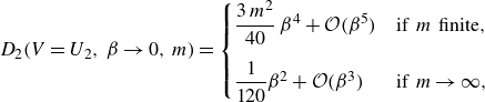 \begin{equation} D_{2}(V=U_{2},\,\beta \to 0,\,m)= \begin{cases} \dfrac {3\,m^2}{40}\,\beta ^{4}+\mathcal{O}(\beta ^{5}) & \text{if}\,\, m\,\,\text{finite}, \\[12pt] \dfrac {1}{120} \beta ^{2}+\mathcal{O} (\beta ^{3}) & \text{if}\,\, m\to \infty, \end{cases} \end{equation}
showing that the shear-induced diffusion becomes negligibly small in thin films. This can be explained by looking at figure 3(d): when $\beta \to 0$
, the speed of the liquid becomes so small that the system is dominated by diffusion.
$\beta \to 0$
, the speed of the liquid becomes so small that the system is dominated by diffusion.
In general, advection and diffusion compete in the transient dynamics described by (3.10). To quantify this, similarly to Dejam et al. (Reference Dejam, Hassanzadeh and Chen2014)and Ling et al. (Reference Ling, Tartakovsky and Battiato2016), we introduce the ratio between the effective diffusivity (3.11a
) and its single phase limit (which corresponds to the analogous of the classical Aris–Taylor dispersion coefficient for the thermal problem), $\mathcal{D}_{{AT}}=1+\frac {2}{105}\,{\textit{Pe}}^{2}$
(Horne & Rodriguez Reference Horne and Rodriguez1983; Berkowitz & Zhou Reference Berkowitz and Zhou1996; Wang et al. Reference Wang, Cardenas, Deng and Bennett2012):
$\mathcal{D}_{{AT}}=1+\frac {2}{105}\,{\textit{Pe}}^{2}$
(Horne & Rodriguez Reference Horne and Rodriguez1983; Berkowitz & Zhou Reference Berkowitz and Zhou1996; Wang et al. Reference Wang, Cardenas, Deng and Bennett2012):
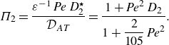 \begin{equation} \Pi _{2}=\dfrac {\varepsilon ^{-1}\,{\textit{Pe}}\,D_{2}^{\star }}{\mathcal{D}_{{AT}}}= \dfrac {1+{\textit{Pe}}^{2}\,D_{2}}{1+\dfrac {2}{105}\,{\textit{Pe}}^{2}}. \end{equation}
This normalisation facilitates the identification of different regimes, based on the competition between diffusion and advection, as shown in figure 4, where the evolution of $\Pi _{2}$
with respect to the Péclet number and the viscosity ratio at two fixed volume fractions,
$\Pi _{2}$
with respect to the Péclet number and the viscosity ratio at two fixed volume fractions, $\beta =\{0.2,\,0.8\}$
, is presented. Interestingly, for small Péclet numbers (
$\beta =\{0.2,\,0.8\}$
, is presented. Interestingly, for small Péclet numbers ( ${\textit{Pe}}\lt 1$
),
${\textit{Pe}}\lt 1$
), $\Pi _{2}\to 1$
and it is independent of
$\Pi _{2}\to 1$
and it is independent of $m$
and
$m$
and $\beta$
, meaning that advective mixing of thermal energy in the outer phase is negligible compared with heat diffusion. When the Péclet number is sufficiently large, the advection dominates and
$\beta$
, meaning that advective mixing of thermal energy in the outer phase is negligible compared with heat diffusion. When the Péclet number is sufficiently large, the advection dominates and $\Pi _{2}$
assumes always values lower than unity. This means that the core-annular flow pattern does not enhance heat diffusion compared with single-phase flow, in particular, when the volume fraction is small. Also, the mechanism of shear-induced diffusion becomes negligible in the free-surface limit (
$\Pi _{2}$
assumes always values lower than unity. This means that the core-annular flow pattern does not enhance heat diffusion compared with single-phase flow, in particular, when the volume fraction is small. Also, the mechanism of shear-induced diffusion becomes negligible in the free-surface limit ( $m\to 0$
) since the velocity in the outer layer is so small that, regardless of the film thickness
$m\to 0$
) since the velocity in the outer layer is so small that, regardless of the film thickness $\beta$
,
$\beta$
, $\Pi _{2}$
approaches zero without reaching a plateau as
$\Pi _{2}$
approaches zero without reaching a plateau as ${\textit{Pe}}\to \infty$
. The regime map in figure 4 can be used in transient multiphase heat-transfer applications to identify a specific set of operational conditions based on fluid and/or flow properties to enhance or reduce heat diffusion.
${\textit{Pe}}\to \infty$
. The regime map in figure 4 can be used in transient multiphase heat-transfer applications to identify a specific set of operational conditions based on fluid and/or flow properties to enhance or reduce heat diffusion.
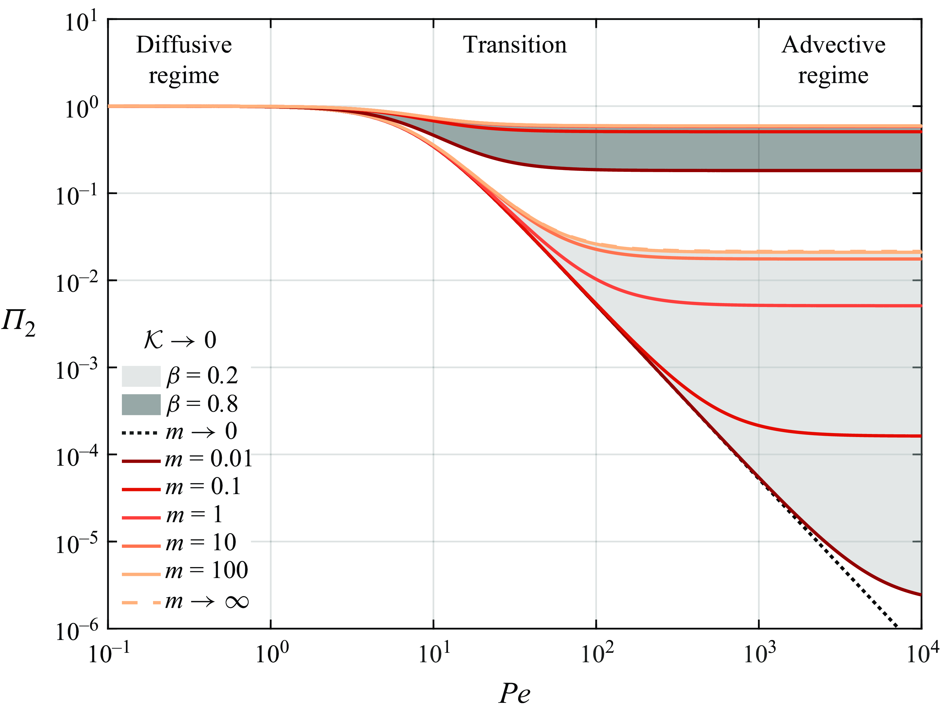
Figure 4. Normalised coefficient of shear-induced thermal diffusivity $\Pi _{2}$
for a decoupled system (
$\Pi _{2}$
for a decoupled system ( $\mathcal{K}\to 0$
) – see definition in (4.2) – against the flow Péclet number
$\mathcal{K}\to 0$
) – see definition in (4.2) – against the flow Péclet number ${\textit{Pe}}$
, for different values of volume fraction
${\textit{Pe}}$
, for different values of volume fraction $\beta$
and viscosity ratio
$\beta$
and viscosity ratio $m$
.
$m$
.
The source term $S_{2}^{\star }$
(3.11b
) is affected by the dimensionless flux
$S_{2}^{\star }$
(3.11b
) is affected by the dimensionless flux $q_{w}$
and the Brinkman number
$q_{w}$
and the Brinkman number ${Br}$
. In particular, it scales with the inverse of the thickness of the outer phase
${Br}$
. In particular, it scales with the inverse of the thickness of the outer phase $S_2^\star \sim q_w/\beta$
, meaning that heating a thin film is very effective since thermal energy is delivered to a small volume of fluid. The viscous dissipation
$S_2^\star \sim q_w/\beta$
, meaning that heating a thin film is very effective since thermal energy is delivered to a small volume of fluid. The viscous dissipation $W_2^\star =W_2^\star (\beta, \,m )$
defined in (C28b, c
), see (C46c
), contributes to the source term, accounting not only for the viscous heating produced in the annulus, but also for the production into the core that is exchanged across the interface. As shown in figure 3(b), in the free-surface limit (
$W_2^\star =W_2^\star (\beta, \,m )$
defined in (C28b, c
), see (C46c
), contributes to the source term, accounting not only for the viscous heating produced in the annulus, but also for the production into the core that is exchanged across the interface. As shown in figure 3(b), in the free-surface limit ( $m\to 0$
), the velocity in the annulus is so slow that viscous dissipation is negligible, while for iso-viscous fluids (
$m\to 0$
), the velocity in the annulus is so slow that viscous dissipation is negligible, while for iso-viscous fluids ( $m=1$
),
$m=1$
), $W_2^\star /\beta =3$
as for single-phase flow. However, in the rigid-core limit (
$W_2^\star /\beta =3$
as for single-phase flow. However, in the rigid-core limit ( $m\to \infty$
), only the outer phase is dissipative and the heat generated due to friction becomes unbounded as the film gets thinner. Due to this singularity around
$m\to \infty$
), only the outer phase is dissipative and the heat generated due to friction becomes unbounded as the film gets thinner. Due to this singularity around $\beta =0$
, the scaling in the thin-film region can be obtained using Laurent series for
$\beta =0$
, the scaling in the thin-film region can be obtained using Laurent series for $\beta \to 0$
as
$\beta \to 0$
as
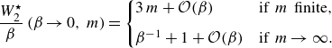 \begin{equation} \dfrac {W_{2}^{\star }}{\beta }\left (\beta \to 0,\,m\right )= \begin{cases} 3\,m+\mathcal{O}(\beta ) & \text{if}\,\, m\,\,\text{finite}, \\[6pt] \beta ^{-1}+1+\mathcal{O}(\beta ) & \text{if}\,\, m\to \infty . \end{cases} \end{equation}
The ADHT equation (3.10) for the decoupled regime admits an analytical solution, setting the initial temperature of the outer phase to a uniform value over the entire channel half-length $x\gt 0$
and imposing the same temperature at the inlet
$x\gt 0$
and imposing the same temperature at the inlet $x=0$
for
$x=0$
for $t\gt 0$
, i.e.
$t\gt 0$
, i.e. $\left \langle \vartheta _{2}\right \rangle (x,\,0 )=\left \langle \vartheta _{2}\right \rangle (0,\,t )\equiv 0$ $\forall \,x,\,t\gt 0,$
we get – see Carslaw & Jaeger (Reference Carslaw and Jaeger1959) and Van Genuchten & Alves (Reference Van Genuchten and Alves1982) –
$\forall \,x,\,t\gt 0,$
we get – see Carslaw & Jaeger (Reference Carslaw and Jaeger1959) and Van Genuchten & Alves (Reference Van Genuchten and Alves1982) –
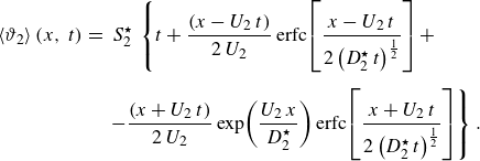 \begin{eqnarray} \left \langle \vartheta _{2}\right \rangle \left (x,\,t\right ) &=& \, S_{2}^{\star }\, \left \{{\vphantom{\left [\frac {x-U_{2}\,t}{2\left (D_{2}^{\star }\,t\right )^{\frac {1}{2}}}\right ]}} t+\frac {(x-U_{2}\,t)}{2\,U_{2}} \operatorname {erfc}\!\left [\frac {x-U_{2}\,t}{2\left (D_{2}^{\star }\,t\right )^{\frac {1}{2}}}\right ] + \right. \nonumber\\[6pt] && \left. -\frac {(x+U_{2}\,t)}{2\,U_{2}} \exp \!\left (\frac {U_{2}\,x}{D_{2}^{\star }}\right ) \operatorname {erfc}\!\left [\frac {x+U_{2}\,t}{2\left (D_{2}^{\star }\,t\right )^{\frac {1}{2}}}\right ]\right \} \,\!. \end{eqnarray}
At long times, the diffusion smears out the temperature profile and the steady-state temperature $\left \langle \vartheta _{2}^{\infty }\right \rangle$
becomes a linear function of
$\left \langle \vartheta _{2}^{\infty }\right \rangle$
becomes a linear function of $x$
(like in classical internal forced-convection problems, see Incropera (Reference Incropera2007)) with slope equal to
$x$
(like in classical internal forced-convection problems, see Incropera (Reference Incropera2007)) with slope equal to $S_{2}^{\star }/ U_{2}$
, i.e.
$S_{2}^{\star }/ U_{2}$
, i.e.
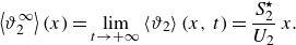 \begin{equation} \left \langle \vartheta _{2}^{\infty }\right \rangle \left (x\right ) = \lim _{t\to +\infty }\left \langle \vartheta _{2}\right \rangle \left (x,\,t\right ) = \frac {S_{2}^{\star }}{U_{2}}\,x. \end{equation}
This solution will be used in § 4.2 to derived a closed-form model for the heat-transfer coefficient. Note that, given the solution for the mean temperature (i.e. its leading order), higher order corrections can be easily calculated plugging (4.4) into (C15), (C23).
4.2. Nusselt number in the decoupled regime
In the decoupled regime, since $\mathcal{K}\to 0$
and
$\mathcal{K}\to 0$
and $\mathcal{K}\,\mathcal{A}\lesssim \varepsilon$
, the bulk temperature (3.15) simplifies to
$\mathcal{K}\,\mathcal{A}\lesssim \varepsilon$
, the bulk temperature (3.15) simplifies to
 \begin{align} \vartheta _{b}\left (x,\,t\right )= \left \langle \vartheta _{2}\right \rangle +\sqrt {\varepsilon }\;U_{2}^{-1}\,{\Big \langle u_{2}(y)\,\vartheta _{2}^{(1)}(y)\Big \rangle }+\mathcal{O}(\varepsilon ). \end{align}
Upon substitution of (4.6) in (3.14), the local Nusselt number (3.14) yields
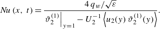 \begin{equation} {\textit{Nu}}\left (x,\,t\right )=\frac {4\,q_{w}/ \sqrt {\varepsilon }}{ \left .\vartheta _{2}^{(1)}\right |_{y=1}-U_{2}^{-1}\,{\left \langle u_{2}(y)\,\vartheta _{2}^{(1)}(y)\right \rangle } }. \end{equation}
Equation (4.7) shows how the Nusselt number evolves in space and time and is calculated by plugging the analytical solution (4.4) into the first-order correction (C15) and using the velocity profile for $u_2(y)$
, given in (A5a
). Here, the Nusselt number is studied with respect to the fixed reference frame, in accordance with the literature, where the bulk temperature is always defined in systems with
$u_2(y)$
, given in (A5a
). Here, the Nusselt number is studied with respect to the fixed reference frame, in accordance with the literature, where the bulk temperature is always defined in systems with $V=0$
.
$V=0$
.
The Nusselt number in laminar decoupled core-annular flows with uniform wall heat flux is a function of space, time, the volume fraction, the viscosity ratio, the dimensionless heat-flux, the Brinkman and the Péclet numbers only, i.e. ${\textit{Nu}}={\textit{Nu}} (x,\,t,\,\beta, \,m,\,q_{w},\,{Br}^{\prime },\,{\textit{Pe}} )$
. The Nusselt number and, as a consequence, the heat-transfer coefficient
${\textit{Nu}}={\textit{Nu}} (x,\,t,\,\beta, \,m,\,q_{w},\,{Br}^{\prime },\,{\textit{Pe}} )$
. The Nusselt number and, as a consequence, the heat-transfer coefficient $h$
depend on the Péclet number only in the transient regime, while at the steady-state,
$h$
depend on the Péclet number only in the transient regime, while at the steady-state, ${\textit{Nu}}^{\infty }={\textit{Nu}}^{\infty } (\beta, \,m,\,{Br}^{\prime } )$
. Note that, as typical in the heat transfer community (Shah & London Reference Shah and London1978), the Péclet number can be seen as the product of the Prandtl and Reynolds numbers, i.e.
${\textit{Nu}}^{\infty }={\textit{Nu}}^{\infty } (\beta, \,m,\,{Br}^{\prime } )$
. Note that, as typical in the heat transfer community (Shah & London Reference Shah and London1978), the Péclet number can be seen as the product of the Prandtl and Reynolds numbers, i.e. ${\textit{Pe}}={Pr}\,{Re}$
, where
${\textit{Pe}}={Pr}\,{Re}$
, where ${Pr}=\mu _{2}/\! (\rho _{2}\,\alpha _{2} )$
and
${Pr}=\mu _{2}/\! (\rho _{2}\,\alpha _{2} )$
and ${Re}=\rho _{2}\,\hat {U}\,\hat {H}/\mu _{2}$
, respectively.
${Re}=\rho _{2}\,\hat {U}\,\hat {H}/\mu _{2}$
, respectively.
When the thermal response reaches the steady state, we get the following expression for the asymptotic Nusselt number ${\textit{Nu}}^{\infty }$
, obtained by combining (4.5), (C15) and (4.7),
${\textit{Nu}}^{\infty }$
, obtained by combining (4.5), (C15) and (4.7),
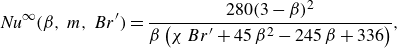 \begin{align} {\textit{Nu}}^{\infty }(\beta, \,m,\,{Br}^{\prime })= \frac {280(3-\beta )^{2}}{\beta \left (\chi \,{Br}^{\prime }+45\,\beta ^2-245\,\beta +336\right )}, \end{align}
where $\chi$
accounts for the contribution of viscous dissipation as
$\chi$
accounts for the contribution of viscous dissipation as
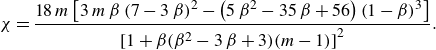 \begin{equation} \chi =\frac {18\,m \left [3\,m\,\beta \left (7 - 3\,\beta \right )^{2} - \left (5\,\beta ^{2} - 35\,\beta + 56\right )\left (1 - \beta \right )^{3}\right ]}{{[1 + \beta (\beta ^{2} - 3\,\beta + 3) (m - 1)]}^{2}}. \end{equation}
Equation (4.8) shows that, in the absence of viscous dissipation ( ${Br}^{\prime }=0$
) or – equivalently – in the inviscid limit (
${Br}^{\prime }=0$
) or – equivalently – in the inviscid limit ( $m\to 0$
), the asymptotic Nusselt number is uniquely a function of the volume fraction of the outer phase
$m\to 0$
), the asymptotic Nusselt number is uniquely a function of the volume fraction of the outer phase $\beta$
. Such an expression embeds the effects of viscous flow in both phases and heat-transfer (advection and diffusion) in the outer phase and it has been obtained starting from first principles. In figure 5(a), the Nusselt number in the non-dissipative regime is represented by the solid black line, which converges to the single phase limit of
$\beta$
. Such an expression embeds the effects of viscous flow in both phases and heat-transfer (advection and diffusion) in the outer phase and it has been obtained starting from first principles. In figure 5(a), the Nusselt number in the non-dissipative regime is represented by the solid black line, which converges to the single phase limit of $140/17$
as
$140/17$
as $\beta \to 1$
. Instead, in the dissipative regime, the single-phase limit of
$\beta \to 1$
. Instead, in the dissipative regime, the single-phase limit of ${\textit{Nu}}^{\infty }$
approaches
${\textit{Nu}}^{\infty }$
approaches $140/\! (108\,{Br}^{\prime }+17 )$
according to (278) of Shah & London (Reference Shah and London1978).
$140/\! (108\,{Br}^{\prime }+17 )$
according to (278) of Shah & London (Reference Shah and London1978).
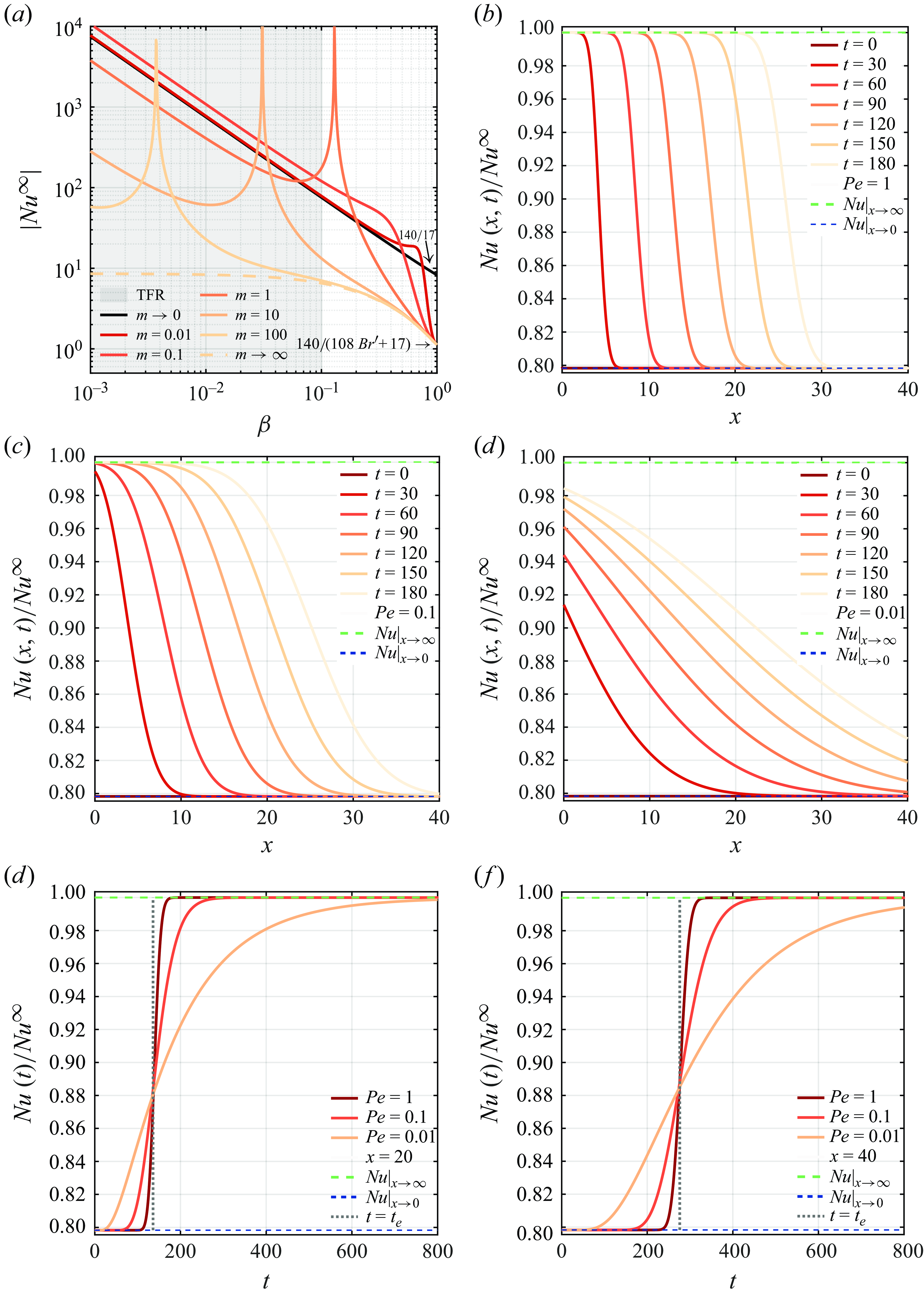
Figure 5. (a) Dependence of the asymptotic Nusselt number ${\textit{Nu}}^{\infty }$
(absolute value) on the volume fraction
${\textit{Nu}}^{\infty }$
(absolute value) on the volume fraction $\beta$
, for fixed viscosity ratios
$\beta$
, for fixed viscosity ratios $m$
and
$m$
and ${Br}^{\prime }=1$
. Evolution of the normalised Nusselt number
${Br}^{\prime }=1$
. Evolution of the normalised Nusselt number ${\textit{Nu}}/{\textit{Nu}}^{\infty }$
: over space at fixed times and Péclet numbers – (b)
${\textit{Nu}}/{\textit{Nu}}^{\infty }$
: over space at fixed times and Péclet numbers – (b) ${\textit{Pe}}=1$
, (c)
${\textit{Pe}}=1$
, (c) ${\textit{Pe}}=0.1$
, (d)
${\textit{Pe}}=0.1$
, (d) ${\textit{Pe}}=0.01$
– over time and across the transport regimes at fixed axial locations – (e)
${\textit{Pe}}=0.01$
– over time and across the transport regimes at fixed axial locations – (e) $x=20$
, (f)
$x=20$
, (f) $x=40$
, with
$x=40$
, with $\varepsilon =0.01$
,
$\varepsilon =0.01$
, ${Br}^{\prime }=0$
,
${Br}^{\prime }=0$
, $q_{w}=\beta =0.1$
,
$q_{w}=\beta =0.1$
, $m=1$
.
$m=1$
.
The viscosity ratio impacts $ {\textit{Nu}}^{\infty }$
only in the dissipative regime, as shown in figure 5(a) for
$ {\textit{Nu}}^{\infty }$
only in the dissipative regime, as shown in figure 5(a) for ${Br}^{\prime }=1$
. Interestingly, when the viscosity ratio
${Br}^{\prime }=1$
. Interestingly, when the viscosity ratio $m$
is sufficiently large (but finite), there exists conditions where viscous heating (
$m$
is sufficiently large (but finite), there exists conditions where viscous heating ( ${Br}^{\prime }\gt 0$
) prevails over the wall heat flux (
${Br}^{\prime }\gt 0$
) prevails over the wall heat flux ( $q_{w}\gt 0$
), and the bulk temperature becomes greater than the wall temperature,
$q_{w}\gt 0$
), and the bulk temperature becomes greater than the wall temperature, $\left .\vartheta _{2}\right |_{y=1}-\vartheta _{b}\lt 0$
, reversing the direction of the heat exchange. When this happens, the heat-transfer coefficient
$\left .\vartheta _{2}\right |_{y=1}-\vartheta _{b}\lt 0$
, reversing the direction of the heat exchange. When this happens, the heat-transfer coefficient $h$
becomes negative, see (3.14), and the singularity of the Nusselt number represents the limiting situation where
$h$
becomes negative, see (3.14), and the singularity of the Nusselt number represents the limiting situation where $\left .\vartheta _{2}\right |_{y=1}=\vartheta _{b}$
. The critical value of volume fraction
$\left .\vartheta _{2}\right |_{y=1}=\vartheta _{b}$
. The critical value of volume fraction $\overline {\beta } = \beta (m,\,{Br}^{\prime } )$
which determines the position of the vertical asymptote can be calculated by finding the zeros of the denominator in (4.8) numerically. To ensure that the Nusselt number remains positive in the entire film thickness range (
$\overline {\beta } = \beta (m,\,{Br}^{\prime } )$
which determines the position of the vertical asymptote can be calculated by finding the zeros of the denominator in (4.8) numerically. To ensure that the Nusselt number remains positive in the entire film thickness range ( $0\lt \beta \lt 1$
), the viscosity ratio and the Brinkman number have to satisfy the inequality
$0\lt \beta \lt 1$
), the viscosity ratio and the Brinkman number have to satisfy the inequality $\chi \,{Br}^{\prime }\gt -91/36$
.
$\chi \,{Br}^{\prime }\gt -91/36$
.
Finally, it is interesting to observe that the asymptotic Nusselt number in the TFR scales as follows:
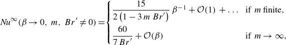 \begin{equation} {\textit{Nu}}^{\infty }(\beta \to 0,\,m,\,{Br}^{\prime }\neq 0)=\! \begin{cases} \dfrac {15}{2 \left (1 - 3\,m\,{Br}^{\prime }\right )}\,\beta ^{-1} + \mathcal{O}(1)\,+ \ldots \!& \text{if}\,\, m\, \text{finite}, \\[12pt] \dfrac {60}{7\,{Br}^{\prime }} + \mathcal{O}(\beta ) & \text{if}\,\, m\to \infty, \end{cases} \end{equation}
while for non-dissipative flows ( ${Br}^{\prime }=0$
), we get that
${Br}^{\prime }=0$
), we get that ${\textit{Nu}}^{\infty }\sim 15/\! (2\,\beta )$
. In the finite-viscosity regimes, the asymptotic Nusselt number
${\textit{Nu}}^{\infty }\sim 15/\! (2\,\beta )$
. In the finite-viscosity regimes, the asymptotic Nusselt number ${\textit{Nu}}^{\infty }$
shows a singularity. Specifically, increasing
${\textit{Nu}}^{\infty }$
shows a singularity. Specifically, increasing $m$
shifts the position of the vertical asymptote towards lower values of
$m$
shifts the position of the vertical asymptote towards lower values of $\beta$
, and a larger number of terms in the expansion (4.10) is required to ensure the convergence of the series to (4.8).
$\beta$
, and a larger number of terms in the expansion (4.10) is required to ensure the convergence of the series to (4.8).
The time and spatial evolution of the local Nusselt number, normalised with respect to its asymptotic value for $t\to \infty$
, i.e.
$t\to \infty$
, i.e. ${\textit{Nu}}/{\textit{Nu}}^{\infty }$
, is shown in figure 5(b–d) for different Péclet numbers. The resulting plots have the form of S-shaped breakthrough curves and they are bounded between two horizontal asymptotes: the upper one denotes the asymptotic Nusselt number, while the lower one corresponds to the Nusselt number predicted by (4.7) at the initial time instant,
${\textit{Nu}}/{\textit{Nu}}^{\infty }$
, is shown in figure 5(b–d) for different Péclet numbers. The resulting plots have the form of S-shaped breakthrough curves and they are bounded between two horizontal asymptotes: the upper one denotes the asymptotic Nusselt number, while the lower one corresponds to the Nusselt number predicted by (4.7) at the initial time instant, $t=0$
. At sufficiently high Péclet numbers, the S-shaped curves are almost rigidly transported by the flow over time, indicating an advective-dominated behaviour; a reduction of the Péclet number leads to a diffusion-dominated regime (see figure 4).
$t=0$
. At sufficiently high Péclet numbers, the S-shaped curves are almost rigidly transported by the flow over time, indicating an advective-dominated behaviour; a reduction of the Péclet number leads to a diffusion-dominated regime (see figure 4).
To determine how the advective and diffusive mechanisms compete in the transient dynamics, we plot the normalised Nusselt number for the different transport regimes considered in figure 5(b–d) over an extended time interval at two fixed positions along the channel: $x=20$
(half-length of the channel) and
$x=20$
(half-length of the channel) and $x=40$
(end of the channel). At high Péclet numbers (
$x=40$
(end of the channel). At high Péclet numbers ( $ {\textit{Pe}}=1$
), the heat is primarily advected downstream and the system quickly reaches the fully developed condition. This means that the heat transfer is quite efficient due to the strong influence of advection. Conversely, decreasing the Péclet number (
$ {\textit{Pe}}=1$
), the heat is primarily advected downstream and the system quickly reaches the fully developed condition. This means that the heat transfer is quite efficient due to the strong influence of advection. Conversely, decreasing the Péclet number ( $ {\textit{Pe}}=\{0.1,\,0.01\}$
) results in a slower increase of the Nusselt number due to the effect of diffusion. An interesting feature in both figures 5(e)
and 5(f) is the existence of a common intersection point between all the curves at
$ {\textit{Pe}}=\{0.1,\,0.01\}$
) results in a slower increase of the Nusselt number due to the effect of diffusion. An interesting feature in both figures 5(e)
and 5(f) is the existence of a common intersection point between all the curves at $t=t_{e}$
that is independent of the value of the Péclet number. For
$t=t_{e}$
that is independent of the value of the Péclet number. For $t\gt t_{e}$
, the Nusselt number increases with the Péclet number, whereas for
$t\gt t_{e}$
, the Nusselt number increases with the Péclet number, whereas for $t\lt t_{e}$
, the behaviour of the system is reversed. At a fixed axial position, the curves appear to pivot around this point.
$t\lt t_{e}$
, the behaviour of the system is reversed. At a fixed axial position, the curves appear to pivot around this point.
4.3. Hierarchy of time scales in thermal dispersion
The trends illustrated in figure 5 also reflect the development of the forced-convective thermal boundary layer, similarly to the single-phase scenario (Siegel & Sparrow Reference Siegel and Sparrow1959; Siegel & Perlmutter Reference Siegel and Perlmutter1963; Fakoor-Pakdaman et al. Reference Fakoor-Pakdaman, Andisheh-Tadbir and Bahrami2014). As time elapses, the thermal boundary layer progressively penetrates and fills up the thickness $\beta$
occupied by the annulus. As a result, increasingly larger distances after
$\beta$
occupied by the annulus. As a result, increasingly larger distances after $x=0$
become thermally fully developed. In fact, since a finite amount of time,
$x=0$
become thermally fully developed. In fact, since a finite amount of time, $t^{\ast }=x^{\ast }/ U_{2}$
, is required for the entrance fluid to be advected downstream and reach the axial position
$t^{\ast }=x^{\ast }/ U_{2}$
, is required for the entrance fluid to be advected downstream and reach the axial position $x^{\ast }$
, beyond this coordinate,
$x^{\ast }$
, beyond this coordinate, $x\geqslant x^{\ast }$
, there has not been any penetration of the fluid which was originally outside the channel before the start of the transient (at
$x\geqslant x^{\ast }$
, there has not been any penetration of the fluid which was originally outside the channel before the start of the transient (at $t=0$
). For
$t=0$
). For $x\lt x^{\ast }$
, the thermal problem reaches its long-time thermal behaviour (linear temperature profile and constant Nusselt number).
$x\lt x^{\ast }$
, the thermal problem reaches its long-time thermal behaviour (linear temperature profile and constant Nusselt number).
Similarly to mass transfer (Allaire, Mikelić & Piatnitski Reference Allaire, Mikelić and Piatnitski2010; Feder, Flekkøy & Hansen Reference Feder, Flekkøy and Hansen2022), the thermal mixing is enhanced in regimes where diffusion has had time to even out the transverse variations of temperature (across the layer) while there are still longitudinal variations at the large scale (along it). Referring to the time scales introduced in § 2.2 and choosing the advective characteristic time scale $\hat {\tau }_{a}$
as the reference time, we obtain the following time scale hierarchy valid for the decoupled model (with
$\hat {\tau }_{a}$
as the reference time, we obtain the following time scale hierarchy valid for the decoupled model (with $j=2$
and
$j=2$
and $\mathcal{K}\to 0$
):
$\mathcal{K}\to 0$
):
 \begin{equation} \tau _{\hat {H},\,2} \ll \tau _{a,\,2} \ll \tau _{\hat {L},\,2}\qquad \Rightarrow \qquad \varepsilon \,{\textit{Pe}}\,\beta ^2 \ll U_{2} \ll \dfrac {{\textit{Pe}}}{\varepsilon }. \end{equation}
By inspection of (4.11), we can conclude that if the channel is sufficiently shallow ( $\varepsilon \to 0$
), these three times scales are sharply separated over a wide range of Péclet numbers, as shown in figure 6. In particular, since the mean velocity of the annulus is bounded between
$\varepsilon \to 0$
), these three times scales are sharply separated over a wide range of Péclet numbers, as shown in figure 6. In particular, since the mean velocity of the annulus is bounded between $0$
and
$0$
and $1$
, i.e.
$1$
, i.e. $0\leqslant {U_{2}}\leqslant 1$
(see figure 3
d), thermal dispersion is observed for times of the order of
$0\leqslant {U_{2}}\leqslant 1$
(see figure 3
d), thermal dispersion is observed for times of the order of $\hat {\tau }_a$
whenever
$\hat {\tau }_a$
whenever ${\textit{Pe}}\gtrsim \varepsilon$
. For smaller Péclet numbers, the problem approaches its purely diffusive limit, where mixing is not influenced by shear-induced mechanisms. Interestingly, in the inviscid limit (
${\textit{Pe}}\gtrsim \varepsilon$
. For smaller Péclet numbers, the problem approaches its purely diffusive limit, where mixing is not influenced by shear-induced mechanisms. Interestingly, in the inviscid limit ( $m\to 0$
), the outer phase is almost at rest (
$m\to 0$
), the outer phase is almost at rest ( $U_{2}\to 0$
) and does not experience any shear-induced mixing, while in the TFR limit, the outer phase is so thin that transverse diffusion is almost instantaneous (
$U_{2}\to 0$
) and does not experience any shear-induced mixing, while in the TFR limit, the outer phase is so thin that transverse diffusion is almost instantaneous ( $\tau _{\hat {H},2}\to 0$
as
$\tau _{\hat {H},2}\to 0$
as $\beta \to 0$
) at any
$\beta \to 0$
) at any $ {\textit{Pe}}$
.
$ {\textit{Pe}}$
.
Finally, it is worth recalling that our analysis cannot describe the early-time dynamics of the system – which may be referred to as pre-asymptotic dispersion regime (Young & Jones Reference Young and Jones1991; Taghizadeh et al. Reference Taghizadeh, Valdés-Parada and Wood2020) – and the upscaled model (3.10) holds only at times that are much greater than $\tau _{\hat {H},\,2}$
, i.e.
$\tau _{\hat {H},\,2}$
, i.e. $t\gg \varepsilon \,{\textit{Pe}}\,\beta ^2$
, holding no memory from the initial conditions (Ananthakrishnan, Gill & Barduhn Reference Ananthakrishnan, Gill and Barduhn1965; Sankarasubramanian, Gill & Benjamin Reference Sankarasubramanian, Gill and Benjamin1973; Fallon & Chauhan Reference Fallon and Chauhan2005).
$t\gg \varepsilon \,{\textit{Pe}}\,\beta ^2$
, holding no memory from the initial conditions (Ananthakrishnan, Gill & Barduhn Reference Ananthakrishnan, Gill and Barduhn1965; Sankarasubramanian, Gill & Benjamin Reference Sankarasubramanian, Gill and Benjamin1973; Fallon & Chauhan Reference Fallon and Chauhan2005).
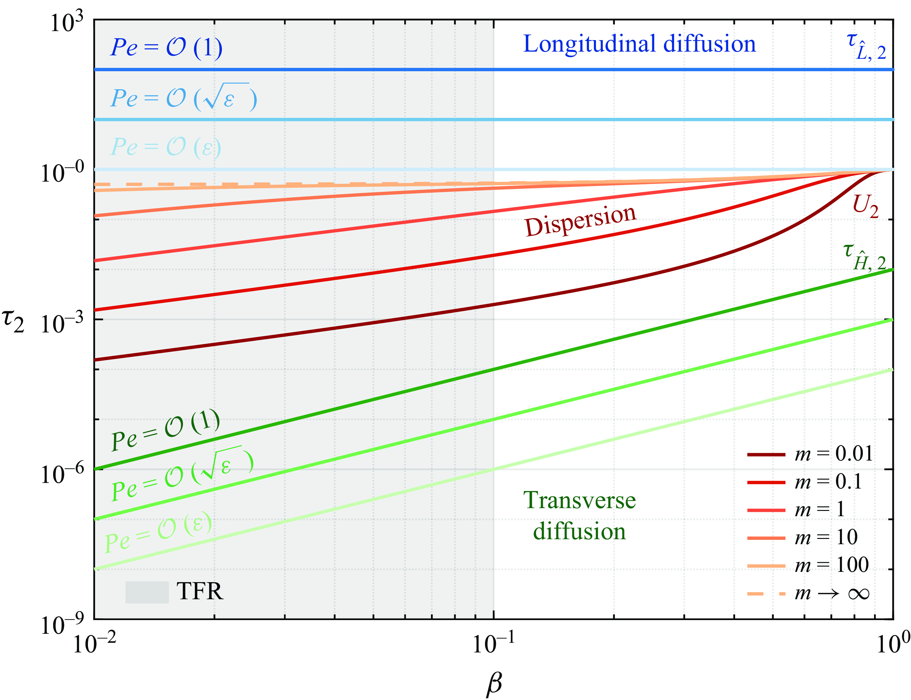
Figure 6. Time scale hierarchy and corresponding dominant heat-transfer mechanisms for the decoupled model ( $\mathcal{K}\to 0$
) as a function of the volume fraction
$\mathcal{K}\to 0$
) as a function of the volume fraction $\beta$
at different viscosity ratio
$\beta$
at different viscosity ratio $m$
and Péclet number
$m$
and Péclet number ${\textit{Pe}}$
.
${\textit{Pe}}$
. $\tau _{2}=\{\tau _{\hat {H},\,2},\,U_{2},\,\tau _{\hat {L},\,2}\}$
are the characteristic times of transverse diffusion, advection (average speed of the annulus) and longitudinal diffusion, see (4.11), respectively. The dispersion regime is characterised by the dynamical competition between longitudinal advection and diffusion.
$\tau _{2}=\{\tau _{\hat {H},\,2},\,U_{2},\,\tau _{\hat {L},\,2}\}$
are the characteristic times of transverse diffusion, advection (average speed of the annulus) and longitudinal diffusion, see (4.11), respectively. The dispersion regime is characterised by the dynamical competition between longitudinal advection and diffusion. $\varepsilon =0.01$
.
$\varepsilon =0.01$
.
4.4. Ramifications for the modelling of thin films and Taylor bubbles
In some circumstances, the modelling of flow patterns, such as intermittent slug flow, relies on an idealisation of the liquid film region, borrowing closure relations from core-annular flows (see for example, Balestra, Zhu & Gallaire (Reference Balestra, Zhu and Gallaire2018); Picchi et al. (Reference Picchi, Ullmann and Brauner2018)). Taylor bubble flow, in fact, consists of a sequence of liquid slugs and elongated bubbles, and – if the bubble is sufficiently long – a region of uniform film thickness forms, which can be considered, as a first approximation, a (local) region of fully developed core-annular flow. This approach neglects the evolution of the thin-film typical of Bretherton’s problem (Bretherton Reference Bretherton1961), while preserving model simplicity. In the context of heat transfer, the widely used three-zone model developed by Thome et al. (Reference Thome, Dupont and Jacobi2004) and Dupont, Thome & Jacobi (Reference Dupont, Thome and Jacobi2004) assumes that the film region of an evaporating/condensing Taylor bubble can be treated in this way.
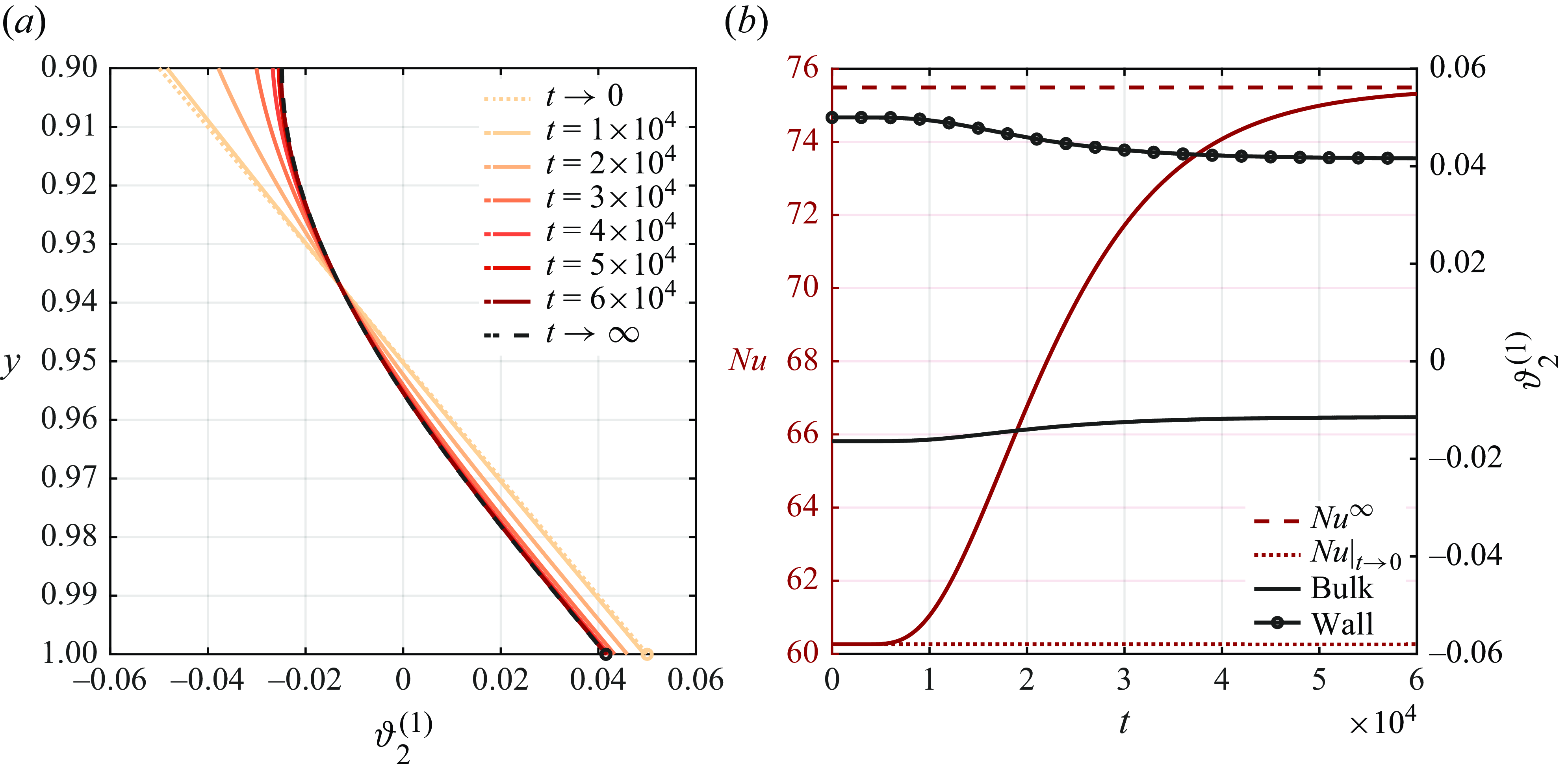
Figure 7. (a) Transient evolution of the first-order correction of the temperature profile of the annulus $\vartheta _{2}^{(1)}$
in the decoupled regime at
$\vartheta _{2}^{(1)}$
in the decoupled regime at $x=40$
, for
$x=40$
, for $\beta =0.1$
,
$\beta =0.1$
, $m=0.01$
,
$m=0.01$
, $\varepsilon =0.01$
,
$\varepsilon =0.01$
, ${\textit{Pe}}=1$
,
${\textit{Pe}}=1$
, $q_{w}=0.1$
and
$q_{w}=0.1$
and ${Br}={Br}^{\prime }=0$
. (b) Right ordinate: time evolution of the wall temperature (
${Br}={Br}^{\prime }=0$
. (b) Right ordinate: time evolution of the wall temperature ( $\vartheta _{2}^{(1)}|_{y=1}$
, black solid lines with circles) and the bulk temperature (
$\vartheta _{2}^{(1)}|_{y=1}$
, black solid lines with circles) and the bulk temperature ( $U_{2}^{-1}\,\langle u_{2}\,\vartheta _{2}^{(1)}\rangle$
, black solid line). Left ordinate: Nusselt number (4.7). The lower asymptote (dotted line) identifies the starting Nusselt number,
$U_{2}^{-1}\,\langle u_{2}\,\vartheta _{2}^{(1)}\rangle$
, black solid line). Left ordinate: Nusselt number (4.7). The lower asymptote (dotted line) identifies the starting Nusselt number, ${Nu}|_{t\to 0}=16(3-\beta )\beta ^{-1}(8-3\,\beta )^{-1}$
; the upper asymptote (dashed line) denotes the fully developed Nusselt number
${Nu}|_{t\to 0}=16(3-\beta )\beta ^{-1}(8-3\,\beta )^{-1}$
; the upper asymptote (dashed line) denotes the fully developed Nusselt number ${Nu}^{\infty }$
(4.8).
${Nu}^{\infty }$
(4.8).
Specifically, the heat transfer coefficient between the thin film surrounding a Taylor bubble and the channel wall is modelled as $h={\kappa _{2}}/{\delta }$
(where
$h={\kappa _{2}}/{\delta }$
(where $\delta$
is the film thickness) considering only the heat conduction in the transverse direction (across the film) at the steady-state and neglecting the impact of advection (see Dupont et al. (Reference Dupont, Thome and Jacobi2004); Thome et al. (Reference Thome, Dupont and Jacobi2004); Dai et al. (Reference Dai, Guo, Fletcher and Haynes2015); Magnini & Thome (Reference Magnini and Thome2017); Zhang & Nikolayev (Reference Zhang and Nikolayev2023)). In this way, the heat-transfer coefficient is obtained by assuming a linear temperature profile in the film. The results presented in § 4.2 can be used to check the validity of this hypothesis. Combining (4.10) with (3.14) and (3.19), we obtain the following scaling law for the steady-state heat-transfer coefficient of core-annular flows in a planar geometry:
$\delta$
is the film thickness) considering only the heat conduction in the transverse direction (across the film) at the steady-state and neglecting the impact of advection (see Dupont et al. (Reference Dupont, Thome and Jacobi2004); Thome et al. (Reference Thome, Dupont and Jacobi2004); Dai et al. (Reference Dai, Guo, Fletcher and Haynes2015); Magnini & Thome (Reference Magnini and Thome2017); Zhang & Nikolayev (Reference Zhang and Nikolayev2023)). In this way, the heat-transfer coefficient is obtained by assuming a linear temperature profile in the film. The results presented in § 4.2 can be used to check the validity of this hypothesis. Combining (4.10) with (3.14) and (3.19), we obtain the following scaling law for the steady-state heat-transfer coefficient of core-annular flows in a planar geometry:
 \begin{equation} h=\dfrac {15}{8}\dfrac {\kappa _2}{\beta \,\hat {H}}. \end{equation}
At the steady-state, $h$
is a function of the fluid conductivity and the film thickness only, i.e.
$h$
is a function of the fluid conductivity and the film thickness only, i.e. $h=h(\kappa _{2},\,\beta \hat {H})$
. Our analysis confirms that the heat-transfer is primarily driven by conduction in the film, and the temperature profile remains almost linear along the transverse direction: when the film is thin enough, the dynamic effects due to the flow are negligible, see figure 3(d),
$h=h(\kappa _{2},\,\beta \hat {H})$
. Our analysis confirms that the heat-transfer is primarily driven by conduction in the film, and the temperature profile remains almost linear along the transverse direction: when the film is thin enough, the dynamic effects due to the flow are negligible, see figure 3(d), $U_2\to 0$
as
$U_2\to 0$
as $\beta \to 0$
. This can be easily shown combining (C15) with the steady-state axial derivative of the averaged temperature (4.4) for
$\beta \to 0$
. This can be easily shown combining (C15) with the steady-state axial derivative of the averaged temperature (4.4) for ${Br}=0$
,
${Br}=0$
,
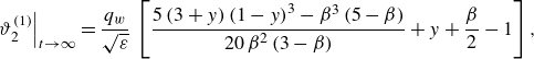 \begin{equation} \left .\vartheta _{2}^{(1)}\right |_{t\to \infty } = \frac {q_{w}}{\sqrt {\varepsilon }}\, \left [\frac {5\left (3 + y\right )\left (1 - y\right )^3 - \beta ^3\left (5-\beta \right )} {20\,\beta ^2\left (3 - \beta \right )} + y + \frac {\beta }{2} - 1\right ], \end{equation}
as plotted in figure 7(a). The temperature profile is almost linear in proximity of the wall, while it flattens out at the interface where the heat-flux is zero; this behaviour is embedded in the numerical factor $15/8$
in (4.12).
$15/8$
in (4.12).
However, in regimes where the film thickness is not small compared with the channel size (Aussillous & Quéré Reference Aussillous and Quéré2000), the flow in the film is not negligible, and the Nusselt number should be estimated using (4.8) instead of (4.12). In addition, accounting for transient effects would introduce the dependence of the Péclet number into the problem – see figure 7(b).
4.5. Heat-transfer mechanisms and temperature field in the coupled regime
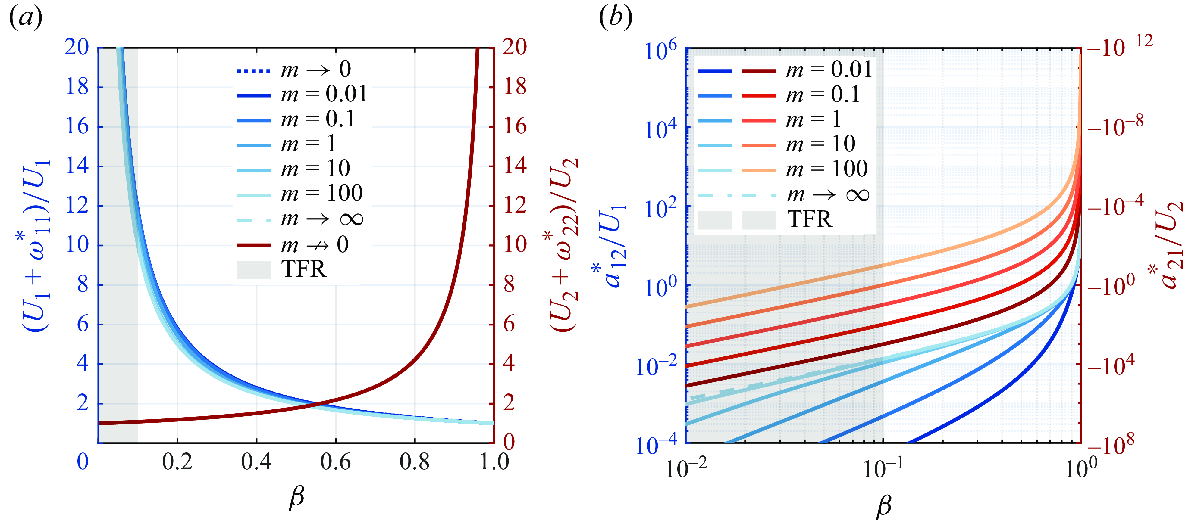
Figure 8. Effective coefficients of advection as functions of the volume fraction $\beta$
, for different viscosity ratios
$\beta$
, for different viscosity ratios $m$
, when
$m$
, when $\mathcal{K}=1$
in the absolute reference frame (
$\mathcal{K}=1$
in the absolute reference frame ( $V=0$
). (a) Advective coefficients normalised with the mean flow speed, i.e.
$V=0$
). (a) Advective coefficients normalised with the mean flow speed, i.e. $a_{jj}^{\star }/{U_{j}}$
:
$a_{jj}^{\star }/{U_{j}}$
: $j=1$
(left) and
$j=1$
(left) and $j=2$
(right). (b) Coefficients of coupled advection
$j=2$
(right). (b) Coefficients of coupled advection $a_{12}^{\star }/{U_{1}}$
(left) and
$a_{12}^{\star }/{U_{1}}$
(left) and $a_{21}^{\star }/{U_{2}}$
(right). Those coefficients are independent of the speed of the reference frame.
$a_{21}^{\star }/{U_{2}}$
(right). Those coefficients are independent of the speed of the reference frame.
When the thermal conductivities of the two phases are of the same order, $\mathcal{K}=\mathcal{O}(1)$
, the heat transfer problem is described by two coupled ADHT equations (3.8), (3.9). Differently from the decoupled regime, the phases can exchange energy through the fluid–fluid interface. By inspection of (3.8), (3.9), we see that the temperatures evolve in time and space due to three different mechanisms: advection, diffusion and storage/source terms. Specifically, each ADHT equation shows (i) a canonical and a coupled effective advection term; (ii) a canonical and a cross-coupling effective diffusion term; (iii) storage and source terms. In the following, we elucidate the physical interpretation of those effective coefficients to describe the main heat-transfer mechanisms of the coupled regime.
$\mathcal{K}=\mathcal{O}(1)$
, the heat transfer problem is described by two coupled ADHT equations (3.8), (3.9). Differently from the decoupled regime, the phases can exchange energy through the fluid–fluid interface. By inspection of (3.8), (3.9), we see that the temperatures evolve in time and space due to three different mechanisms: advection, diffusion and storage/source terms. Specifically, each ADHT equation shows (i) a canonical and a coupled effective advection term; (ii) a canonical and a cross-coupling effective diffusion term; (iii) storage and source terms. In the following, we elucidate the physical interpretation of those effective coefficients to describe the main heat-transfer mechanisms of the coupled regime.
The evolution of the advection coefficient $a_{jj}^{\star }=U_{j}+\omega _{jj}^{\star }$
is shown in figure 8(a) in the fixed reference frame (
$a_{jj}^{\star }=U_{j}+\omega _{jj}^{\star }$
is shown in figure 8(a) in the fixed reference frame ( $V=0$
). For each phase, the advection can be written as the sum of the mean phase velocity and an extra contribution due to phase coupling. When
$V=0$
). For each phase, the advection can be written as the sum of the mean phase velocity and an extra contribution due to phase coupling. When $\beta$
is small, the lubrication effect of the thin annulus enhances the effective advection of the core that scales as
$\beta$
is small, the lubrication effect of the thin annulus enhances the effective advection of the core that scales as $\beta ^{-1}$
and it is not affected by the viscosity ratio. The coupling advective coefficients
$\beta ^{-1}$
and it is not affected by the viscosity ratio. The coupling advective coefficients $a_{ij}^{\star }$
appear in each ADHT due to the continuity of temperature at the fluid–fluid interface (see § C.5.2) and link one phase with the advection of the other one. Those coupling coefficients are plotted in figure 8(b): when
$a_{ij}^{\star }$
appear in each ADHT due to the continuity of temperature at the fluid–fluid interface (see § C.5.2) and link one phase with the advection of the other one. Those coupling coefficients are plotted in figure 8(b): when $\beta$
is small (in the TFR), the coupled advection in the core becomes negligible,
$\beta$
is small (in the TFR), the coupled advection in the core becomes negligible, $a_{12}^{\star }\to 0$
, and, therefore, axial temperature gradients of the annulus do not directly affect the core. Instead, regardless of the value of
$a_{12}^{\star }\to 0$
, and, therefore, axial temperature gradients of the annulus do not directly affect the core. Instead, regardless of the value of $\beta$
,
$\beta$
, $a_{21}^{\star }\to 0$
in the rigid-core limit (for
$a_{21}^{\star }\to 0$
in the rigid-core limit (for $m\to \infty$
), where the velocity profile in the core is almost flat, see figure 3(c), and does not trigger any coupled advection mechanism.
$m\to \infty$
), where the velocity profile in the core is almost flat, see figure 3(c), and does not trigger any coupled advection mechanism.
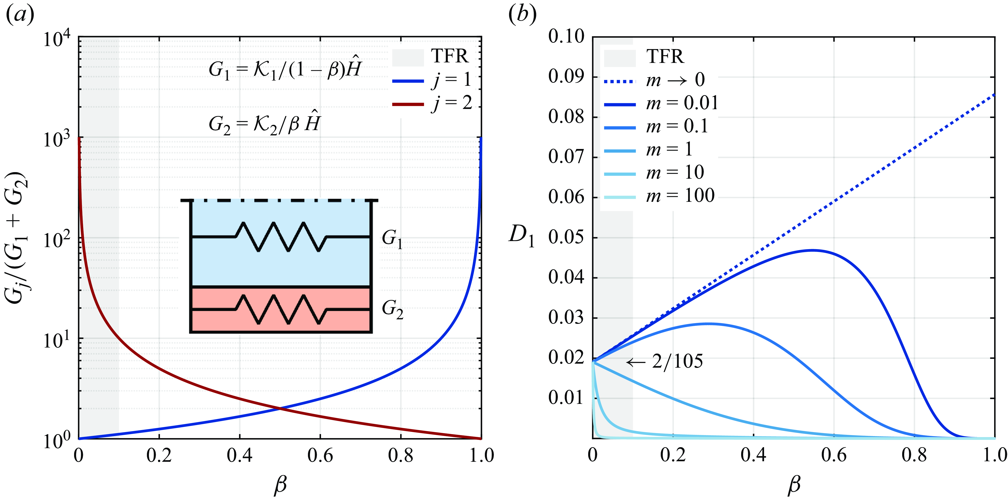
Figure 9. (a) Conductance ratios $G_{j}/ G_{{eq}}$
as functions of the volume fraction
$G_{j}/ G_{{eq}}$
as functions of the volume fraction $\beta$
, for
$\beta$
, for $\mathcal{K}=1$
. (b) Effective coefficients of diffusion as functions of
$\mathcal{K}=1$
. (b) Effective coefficients of diffusion as functions of $\beta$
, for different values of the viscosity ratio
$\beta$
, for different values of the viscosity ratio $m$
, when
$m$
, when $\mathcal{K}=1$
, in the reference frame moving at the mean flow speed (
$\mathcal{K}=1$
, in the reference frame moving at the mean flow speed ( $V=1$
).
$V=1$
).
To investigate the diffusive mechanisms, we can think of heat transfer in the flowing phases via an electrical circuit analogy, as shown in figure 9(a). Specifically, the core-annular flow is represented by a parallel connection of resistors with a specific thermal conductance equal to $G_{1}$
and
$G_{1}$
and $G_2$
; the equivalent conductance is then
$G_2$
; the equivalent conductance is then $G_{\text{eq}}=G_{1}+G_{2}$
. In this framework, we can recast the diffusive coefficients in analogy with the Aris–Taylor formalism to highlight the contribution of heat- and shear-induced diffusion as
$G_{\text{eq}}=G_{1}+G_{2}$
. In this framework, we can recast the diffusive coefficients in analogy with the Aris–Taylor formalism to highlight the contribution of heat- and shear-induced diffusion as
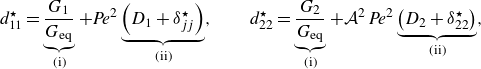 \begin{equation} d_{11}^{\star }=\underbrace {\frac {G_{1}}{G_{\text{eq}}}}_{\textrm {(i)}}+{\textit{Pe}}^{2}\underbrace {\left (D_{1}+\delta _{jj}^{\star }\right )}_{\textrm {(ii)}}, \quad \quad d_{22}^{\star }=\underbrace {\frac {G_{2}}{G_{\text{eq}}}}_{\textrm {(i)}}+\mathcal{A}^{2}\,{\textit{Pe}}^{2}\underbrace {\left (D_{2}+\delta _{22}^{\star }\right )}_{\textrm {(ii)}}, \end{equation}
The first contribution, (i), is a volume-weighted average of the thermal conductivities of the individual phases and recalls the typical effective description proposed by Maxwell for the heat diffusion coefficient of composites (Maxwell Reference Maxwell1873); its evolution with the volume fraction is shown figure 9(a), where we set $\mathcal{K}=1$
. Note that the ratio
$\mathcal{K}=1$
. Note that the ratio $G_{j}/ G_{\text{eq}}$
also appears in front of each time term in (3.8), (3.9), representing the thermal inertia of the phases, i.e. their capacity to store heat and delay its transmission. In the limit of
$G_{j}/ G_{\text{eq}}$
also appears in front of each time term in (3.8), (3.9), representing the thermal inertia of the phases, i.e. their capacity to store heat and delay its transmission. In the limit of $\mathcal{K}\to 0$
, the ratio
$\mathcal{K}\to 0$
, the ratio $G_{2}/ G_{\text{eq}}$
equals unity and the coefficient reduces to one discussed for the decoupled model. The second contribution in the effective diffusive coefficients, (ii), accounts for the shear-induced diffusion,
$G_{2}/ G_{\text{eq}}$
equals unity and the coefficient reduces to one discussed for the decoupled model. The second contribution in the effective diffusive coefficients, (ii), accounts for the shear-induced diffusion, $D_1$
and
$D_1$
and $D_2$
, and the coupling between the phases via the terms
$D_2$
, and the coupling between the phases via the terms $\delta _{jj}^{\star }$
. Both the effective diffusion coefficients scale with the square of the Péclet number, while the extra contribution due to the interaction is specific of this class of coupled-layers problems since it enter the ADHT equations by imposing the continuity of temperatures at the fluid–fluid interface (see the derivation in § C.5.2). Those terms are quadratic expressions in the speed of the moving reference frame,
$\delta _{jj}^{\star }$
. Both the effective diffusion coefficients scale with the square of the Péclet number, while the extra contribution due to the interaction is specific of this class of coupled-layers problems since it enter the ADHT equations by imposing the continuity of temperatures at the fluid–fluid interface (see the derivation in § C.5.2). Those terms are quadratic expressions in the speed of the moving reference frame, $V$
, see (C41), consistent with previous works in the context of mass diffusion, e.g. see Aris (Reference Aris1959).
$V$
, see (C41), consistent with previous works in the context of mass diffusion, e.g. see Aris (Reference Aris1959).
The evolution of $D_{2}$
with
$D_{2}$
with $\beta$
and
$\beta$
and $m$
has been discussed in § 4.1, figure 3(a), while the shear-induced diffusion for the core,
$m$
has been discussed in § 4.1, figure 3(a), while the shear-induced diffusion for the core, $D_{1}$
, is plotted in figure 9(b) setting
$D_{1}$
, is plotted in figure 9(b) setting $V=1$
. Specifically, in the rigid-core limit,
$V=1$
. Specifically, in the rigid-core limit, $m\to \infty$
, the shear-induced diffusion becomes negligible since the inner phase has a flat velocity profile, see figure 3(c), preventing any extra spreading across the axial direction rather than heat diffusion. Conversely, in the free-surface limit,
$m\to \infty$
, the shear-induced diffusion becomes negligible since the inner phase has a flat velocity profile, see figure 3(c), preventing any extra spreading across the axial direction rather than heat diffusion. Conversely, in the free-surface limit, $m\to 0$
, the outer phase is almost at rest and behaves like a static coating:
$m\to 0$
, the outer phase is almost at rest and behaves like a static coating: $D_{1}$
increases linearly with the thickness
$D_{1}$
increases linearly with the thickness $\beta$
as
$\beta$
as
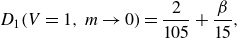 \begin{equation} D_{1}(V=1,\,m\to 0)=\dfrac {2}{105} + \dfrac {\beta }{15}, \end{equation}
showing that a thinner core will result in higher transverse variations in its velocity profile, promoting the shear-induced axial diffusion mechanism. As expected, the single-phase limit of $2/105$
is recovered when
$2/105$
is recovered when $\beta \to 0$
.
$\beta \to 0$
.
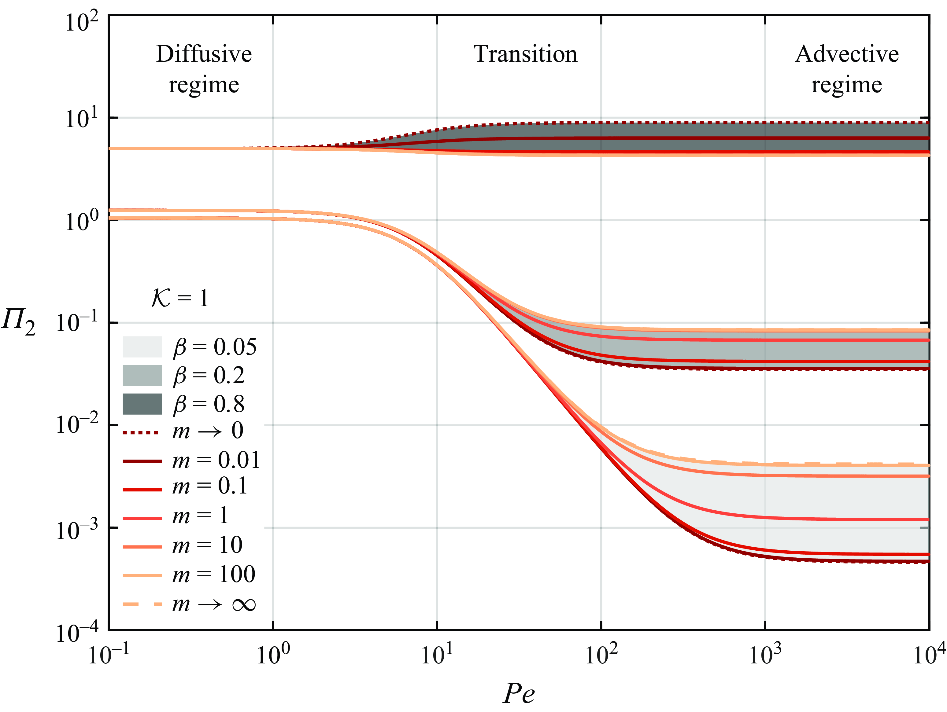
Figure 10. Normalised coefficient of shear-induced thermal conductivity $\Pi _{2}$
for the outer phase of core-annular flows (
$\Pi _{2}$
for the outer phase of core-annular flows ( $\mathcal{K}=1$
) against the flow Péclet number
$\mathcal{K}=1$
) against the flow Péclet number ${\textit{Pe}}$
, for different values of volume fraction
${\textit{Pe}}$
, for different values of volume fraction $\beta$
and viscosity ratio
$\beta$
and viscosity ratio $m$
.
$m$
.
To explore the influence of the flow parameters ( $m$
,
$m$
, $\beta$
,
$\beta$
, ${\textit{Pe}}$
,
${\textit{Pe}}$
, $\mathcal{K}$
,
$\mathcal{K}$
, $\mathcal{A}$
) on the heat-transfer mechanisms in the coupled regime, we set
$\mathcal{A}$
) on the heat-transfer mechanisms in the coupled regime, we set $V=1$
and study the ratio between the coefficient of shear-induced thermal diffusivity in (4.14) and its single-phase limit,
$V=1$
and study the ratio between the coefficient of shear-induced thermal diffusivity in (4.14) and its single-phase limit, $\Pi _{j}={d_{jj}^{\star }}/{\mathcal{D}_{\text{AT},\,j}}$
, similarly to what done in § 4.1:
$\Pi _{j}={d_{jj}^{\star }}/{\mathcal{D}_{\text{AT},\,j}}$
, similarly to what done in § 4.1:
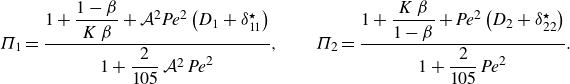 \begin{equation} \Pi _{1} = \dfrac {1+\dfrac {1-\beta }{K\,\beta }+\mathcal{A}^{2}{\textit{Pe}}^{2} \left (D_{1}+\delta _{11}^{\star }\right )} {1+\dfrac {2}{105}\,\mathcal{A}^{2}\,{\textit{Pe}}^{2}}, \quad \quad \Pi _{2} = \dfrac {1+\dfrac {K\,\beta }{1-\beta }+{\textit{Pe}}^{2} \left (D_{2}+\delta _{22}^{\star }\right )} {1+\dfrac {2}{105}\,{\textit{Pe}}^{2}}. \end{equation}
The evolution of $\Pi _{2}$
against the Péclet number is shown in figure 10, varying the viscosity ratio
$\Pi _{2}$
against the Péclet number is shown in figure 10, varying the viscosity ratio $m$
for three different volume fractions
$m$
for three different volume fractions $\beta =\{0.05,\,0.2,\,0.8\}$
; the conductivity ratio
$\beta =\{0.05,\,0.2,\,0.8\}$
; the conductivity ratio $\mathcal{K}$
has been set to unity. The normalised diffusion coefficient of the outer phase has the form of an S-shaped curve and allows the identification of a diffusion-dominated and an advection-dominated regime. Differently from the decoupled model, the purely diffusive regime is characterised by a limiting value that exceeds unity, i.e.
$\mathcal{K}$
has been set to unity. The normalised diffusion coefficient of the outer phase has the form of an S-shaped curve and allows the identification of a diffusion-dominated and an advection-dominated regime. Differently from the decoupled model, the purely diffusive regime is characterised by a limiting value that exceeds unity, i.e. $\Pi _{2}\to 1+K\,\beta /{ (1-\beta )}$
for
$\Pi _{2}\to 1+K\,\beta /{ (1-\beta )}$
for ${\textit{Pe}}\to 0$
, and equal to the conductance ratio
${\textit{Pe}}\to 0$
, and equal to the conductance ratio $G_{2}/{G_{\text{eq}}}$
, see the expression of
$G_{2}/{G_{\text{eq}}}$
, see the expression of $t_{2}^{\star }$
given in (C38). The advective limit is strongly affected by the viscosity ratio and the volume fractions. Specifically, when the thickness
$t_{2}^{\star }$
given in (C38). The advective limit is strongly affected by the viscosity ratio and the volume fractions. Specifically, when the thickness $\beta$
is small, the combined effect of advection and the coupling between phases reduces the diffusion coefficients compared with the case of single-phase flow. This effect is more pronounced in the free-surface than in the rigid-core limit. When the annulus is thick enough, instead,
$\beta$
is small, the combined effect of advection and the coupling between phases reduces the diffusion coefficients compared with the case of single-phase flow. This effect is more pronounced in the free-surface than in the rigid-core limit. When the annulus is thick enough, instead, $\Pi _{2}$
can overcome the purely diffusive limit for sufficiently small values of the viscosity ratio
$\Pi _{2}$
can overcome the purely diffusive limit for sufficiently small values of the viscosity ratio $m$
. The shear-induced diffusion ratio for the inner phase
$m$
. The shear-induced diffusion ratio for the inner phase $\Pi _{1}$
shows a similar behaviour, as presented in figure 11: at low Péclet numbers,
$\Pi _{1}$
shows a similar behaviour, as presented in figure 11: at low Péclet numbers, $\Pi _{1}\to G_{1}/{G_{\text{eq}}}=1+ (1-\beta )/ (K\,\beta )$
, see the expression of
$\Pi _{1}\to G_{1}/{G_{\text{eq}}}=1+ (1-\beta )/ (K\,\beta )$
, see the expression of $t_{1}^{\star }$
given in (C38). However, in the advective regime, the shear-induced diffusion in the core is minimal in the rigid-core limit, where transverse variations of velocity are negligible.
$t_{1}^{\star }$
given in (C38). However, in the advective regime, the shear-induced diffusion in the core is minimal in the rigid-core limit, where transverse variations of velocity are negligible.
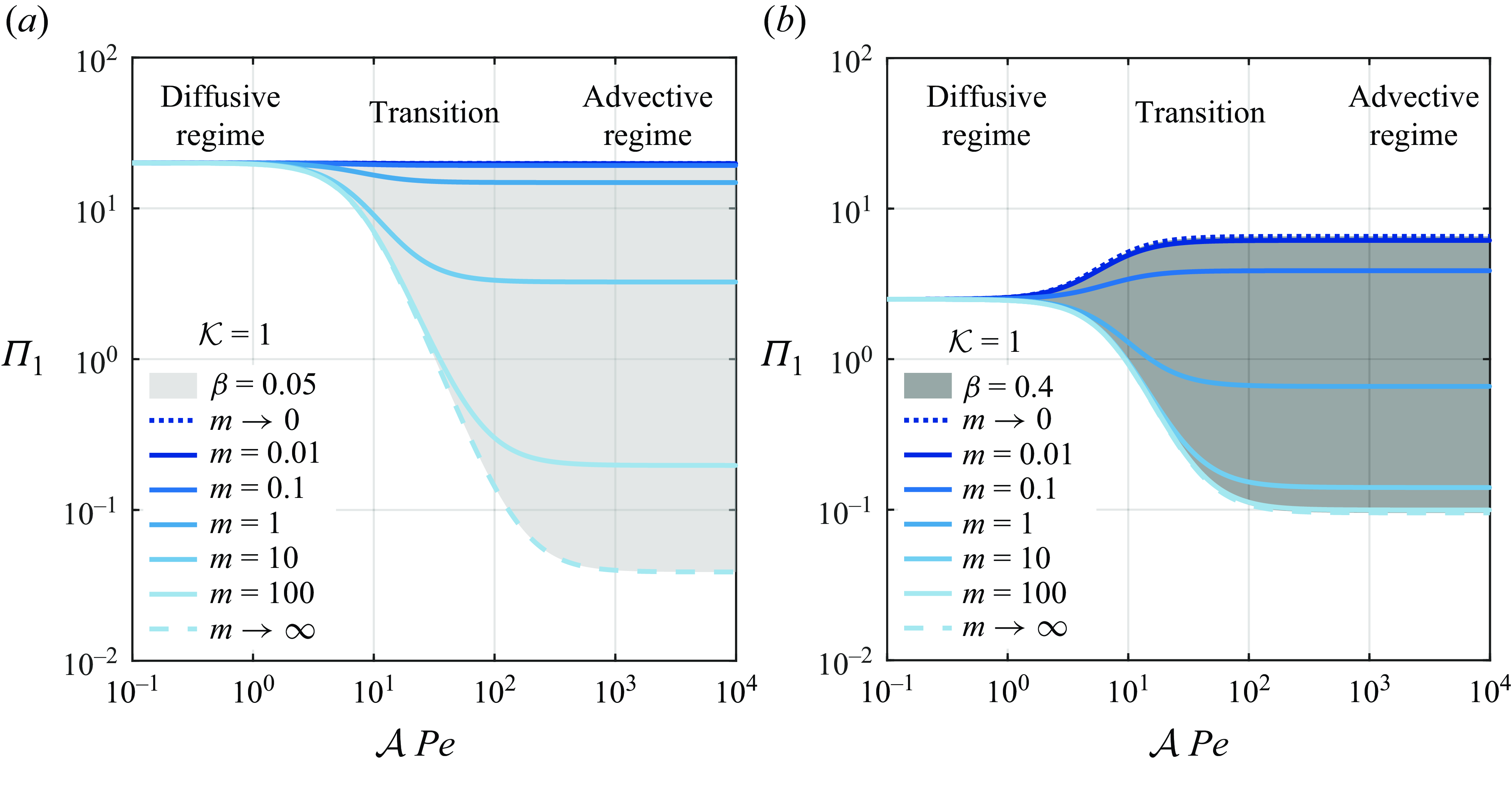
Figure 11. Normalised coefficient of shear-induced thermal diffusivity $\Pi _{1}$
for the inner phase of core-annular flows (
$\Pi _{1}$
for the inner phase of core-annular flows ( $\mathcal{K}=1$
) against the flow Péclet number
$\mathcal{K}=1$
) against the flow Péclet number $\mathcal{A}\,{\textit{Pe}}$
, for different values of viscosity ratio
$\mathcal{A}\,{\textit{Pe}}$
, for different values of viscosity ratio $m$
, setting the volume fraction to (a)
$m$
, setting the volume fraction to (a) $\beta =0.05$
and (b)
$\beta =0.05$
and (b) $\beta =0.4$
.
$\beta =0.4$
.
A similar analysis can be done for the cross-coupling diffusive terms ${\textit{Pe}}^{2}\,d_{12}^{\star }$
and
${\textit{Pe}}^{2}\,d_{12}^{\star }$
and $\mathcal{A}^{2}\,{\textit{Pe}}^{2}\,d_{21}^{\star }$
in (3.8), (3.9), introducing the following ratios:
$\mathcal{A}^{2}\,{\textit{Pe}}^{2}\,d_{21}^{\star }$
in (3.8), (3.9), introducing the following ratios:
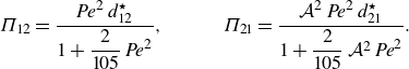 \begin{equation} \Pi _{12}=\dfrac {{\textit{Pe}}^{2}\,d_{12}^{\star }}{1+\dfrac {2}{105}\,{\textit{Pe}}^{2}},\qquad \quad \Pi _{21}=\dfrac {\mathcal{A}^{2}\,{\textit{Pe}}^{2}\,d_{21}^{\star }}{1+\dfrac {2}{105}\,\mathcal{A}^{2}\,{\textit{Pe}}^{2}}. \end{equation}
The physical origin of these coupling terms is due to advection only, as can be seen in figure 12. Both coefficients, in fact, tend to zero in the purely diffusive regime ( ${\textit{Pe}}\to 0$
) and play a role only when advection is important, i.e. at high Péclet numbers. Note that the coupling terms enter the model when the temperature continuity is enforced, see Appendix C.5.2, suggesting that, at high Péclet numbers, heat diffusion in one phase is influenced by diffusion in the other one and vice versa. This mechanism can either play as negative diffusion (with respect to a reference frame that moves with the mean flow
${\textit{Pe}}\to 0$
) and play a role only when advection is important, i.e. at high Péclet numbers. Note that the coupling terms enter the model when the temperature continuity is enforced, see Appendix C.5.2, suggesting that, at high Péclet numbers, heat diffusion in one phase is influenced by diffusion in the other one and vice versa. This mechanism can either play as negative diffusion (with respect to a reference frame that moves with the mean flow $V=1$
, and, therefore, the core is always faster than the annulus), as in the case of the annulus, see figure 12(a), or either enhance or reduce diffusion depending on
$V=1$
, and, therefore, the core is always faster than the annulus), as in the case of the annulus, see figure 12(a), or either enhance or reduce diffusion depending on $m$
and
$m$
and $\beta$
in the case of the core, see figure 12(b).
$\beta$
in the case of the core, see figure 12(b).
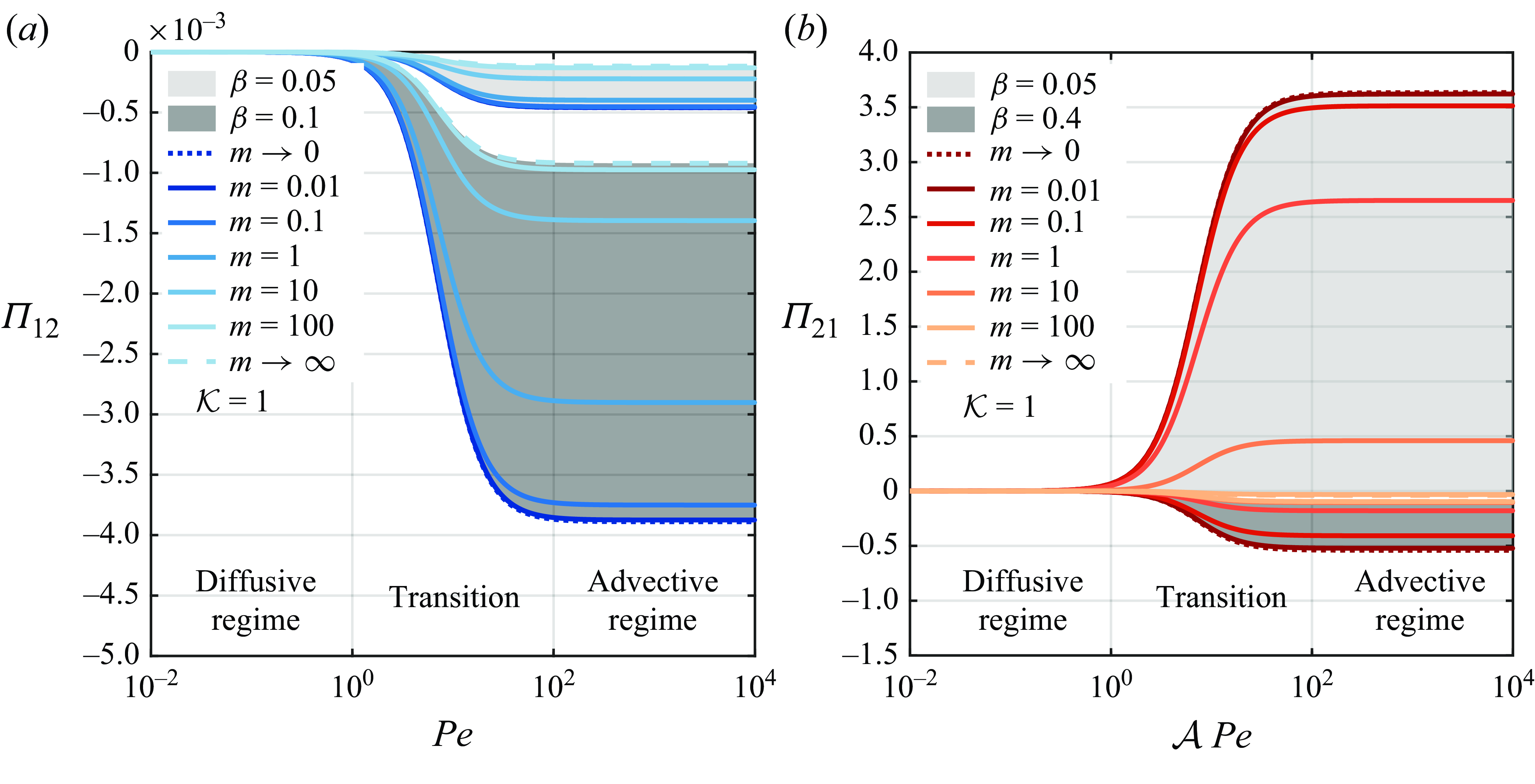
Figure 12. Normalised coefficients of cross-coupling diffusivity, (a) $\Pi _{12}$
and (b)
$\Pi _{12}$
and (b) $\Pi _{21}$
, for a core-annular system (
$\Pi _{21}$
, for a core-annular system ( $\mathcal{K}=1$
) against the corresponding flow Péclet number, for different values of viscosity ratio
$\mathcal{K}=1$
) against the corresponding flow Péclet number, for different values of viscosity ratio $m$
and volume fraction
$m$
and volume fraction $\beta$
.
$\beta$
.
Finally, we study the source terms in (3.8), (3.9) to interpret how the external source of energy $q_w$
affects the model. To do so, observing that the source terms are identical up to a factor equal to
$q_w$
affects the model. To do so, observing that the source terms are identical up to a factor equal to $K^2$
, i.e.
$K^2$
, i.e. $K^{2}\,e_{1}^{\star }=e_{2}^{\star }$
, see (C45), and are opposite-signed, we consider the linear combination,
$K^{2}\,e_{1}^{\star }=e_{2}^{\star }$
, see (C45), and are opposite-signed, we consider the linear combination, $K^{2}$
(3.8) + (3.9), so that the exchange terms cancel out to obtain
$K^{2}$
(3.8) + (3.9), so that the exchange terms cancel out to obtain
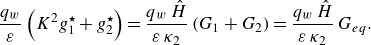 \begin{equation} \frac {q_{w}}{\varepsilon }\left (K^{2} g_{1}^{\star }+g_{2}^{\star }\right )= \frac {q_{w}\,\hat {H}}{\varepsilon \,\kappa _{2}}\left (G_{1}+G_{2}\right )= \frac {q_{w}\,\hat {H}}{\varepsilon \,\kappa _{2}}\,G_{{eq}}. \end{equation}
The resulting source term is the imposed heat flux at the channel wall multiplied by the sum of the two thermal conductances, see figure 9(a), confirming the consistency of our model. In other words, in the equation for the annulus, the source term is positive and greater with respect to the decoupled model by a factor ${3\,K}/{2 (1-\beta )}\gt 0$
– see (C44) – while in the core, the source term is negative,
${3\,K}/{2 (1-\beta )}\gt 0$
– see (C44) – while in the core, the source term is negative, $-K/{2 (1-\beta )}\lt 0$
, so as to preserve the continuity of the temperature and the thermal flux across the interface. Overall, the energy entering both layers is equal to (4.18) and consistent with the imposed boundary conditions (2.16).
$-K/{2 (1-\beta )}\lt 0$
, so as to preserve the continuity of the temperature and the thermal flux across the interface. Overall, the energy entering both layers is equal to (4.18) and consistent with the imposed boundary conditions (2.16).
4.6. Transient and steady-state temperature field in the coupled regime
In the coupled regime, the system of coupled ADHT equations (3.8), (3.9) can be solved numerically and admits an analytical solution only at the steady state.
At the steady state, in fact, diffusion smears out any sharp differences of temperature, and the solution $\langle \vartheta _{j}^{\infty }\rangle (x)$
,
$\langle \vartheta _{j}^{\infty }\rangle (x)$
, $j=\{1,\,2\}$
, can be derived by setting to zero the time derivatives and diffusive terms in (3.8), (3.9), yielding an inhomogeneous system of linear first-order ordinary differential equations (ODEs), which can be recast via a linear combination as
$j=\{1,\,2\}$
, can be derived by setting to zero the time derivatives and diffusive terms in (3.8), (3.9), yielding an inhomogeneous system of linear first-order ordinary differential equations (ODEs), which can be recast via a linear combination as
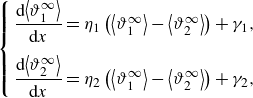 \begin{align} \left \{ \begin{array}{ll}\dfrac{\textrm {d}{\left \langle \vartheta _{1}^{\infty }\right \rangle }}{\textrm{d}x} = \eta _{1} \left(\left \langle \vartheta _{1}^{\infty }\right \rangle -\left \langle \vartheta _{2}^{\infty }\right \rangle \right ) + \gamma _{1},\\[12pt] \dfrac{\textrm {d}{\left \langle \vartheta _{2}^{\infty }\right \rangle }}{\textrm{d} x} = \eta _{2} \left (\left \langle \vartheta _{1}^{\infty }\right \rangle -\left \langle \vartheta _{2}^{\infty }\right \rangle \right ) + \gamma _{2},\end{array} \right . \end{align}
where
 \begin{gather} \lambda =\varepsilon \left (a_{11}^{\star }\,a_{22}^{\star }-a_{12}^{\star }\,a_{21}^{\star }\right ),\quad \eta _{1}=-\frac {a_{22}^{\star }\,e_{1}^{\star }+a_{12}^{\star }\,e_{2}^{\star }}{\mathcal{A}\,{\textit{Pe}}\,\lambda },\quad \eta _{2}=\frac {a_{21}^{\star }\,e_{1}^{\star }+a_{11}^{\star }\,e_{2}^{\star }}{{\textit{Pe}}\,\lambda }, \end{gather}
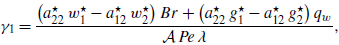 \begin{gather} \gamma _{1}=\frac {\left (a_{22}^{\star }\,w_{1}^{\star }-a_{12}^{\star }\,w_{2}^{\star }\right ){Br}+ \left (a_{22}^{\star }\,g_{1}^{\star }-a_{12}^{\star }\,g_{2}^{\star }\right )q_{w}}{\mathcal{A}\,{\textit{Pe}}\,\lambda }, \end{gather}
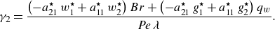 \begin{gather} \gamma _{2}=\frac {\left (-a_{21}^{\star }\,w_{1}^{\star }+a_{11}^{\star }\,w_{2}^{\star }\right ){Br}+ \left (-a_{21}^{\star }\,g_{1}^{\star }+a_{11}^{\star }\,g_{2}^{\star }\right )q_{w}}{{\textit{Pe}}\,\lambda }. \end{gather}
A particular solution to system (4.19) (see Kamke (Reference Kamke1977); Polyanin & Zaitsev (Reference Polyanin and Zaitsev2017)) is represented by two parallel lines of slope $M$
and intercepts
$M$
and intercepts $Q_{j}$
:
$Q_{j}$
:
 \begin{equation} \big\langle \vartheta _{j}^{\infty }\big\rangle \left (x\right )=Mx+Q_{j},\quad \text{with} \quad M=\frac {\eta _{1}\,\gamma _{2}-\eta _{2}\,\gamma _{1}}{\eta _{1}-\eta _{2}}, \quad Q_{j}=-\frac {\eta _{j}\left (\gamma _{1}-\gamma _{2}\right )}{\left (\eta _{1}-\eta _{2}\right )^{2}}, \end{equation}
meaning that, at the steady state, the temperature of both phases increases linearly in the axial direction with slope equal to $M(q_{w}/{\textit{Pe}},\,\beta, \,m,\,\mathcal{K}\,\mathcal{A},\,{Br}^{\prime })$
given by
$M(q_{w}/{\textit{Pe}},\,\beta, \,m,\,\mathcal{K}\,\mathcal{A},\,{Br}^{\prime })$
given by
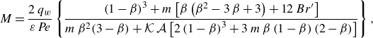 \begin{equation} M = \frac {2\,q_{w}}{\varepsilon \,{\textit{Pe}}}\left \{\frac {\left (1-\beta \right )^3+m\left [\beta \left (\beta ^2 - 3\,\beta +3\right )+12\,{Br}^{\prime }\right ]}{m\,\beta ^2(3-\beta )+\mathcal{K}\,\mathcal{A}\left [2\left (1-\beta \right )^3+3\,m\,\beta \left (1-\beta \right )(2-\beta)\right ]}\right \}, \end{equation}
where the dimensionless group $\mathcal{K}\,\mathcal{A}$
represents the volumetric heat capacity ratio. Remarkably, in the free-surface limit,
$\mathcal{K}\,\mathcal{A}$
represents the volumetric heat capacity ratio. Remarkably, in the free-surface limit, $m\to 0$
,
$m\to 0$
, $M$
is independent of
$M$
is independent of $\beta$
and equals
$\beta$
and equals $q_{w}/(\varepsilon \,{\textit{Pe}}\,\mathcal{K}\,\mathcal{A})$
, whereas the single-phase limits are
$q_{w}/(\varepsilon \,{\textit{Pe}}\,\mathcal{K}\,\mathcal{A})$
, whereas the single-phase limits are
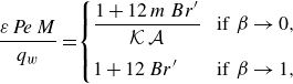 \begin{equation} \frac {\varepsilon \,{\textit{Pe}}\,M}{q_{w}} =\! \begin{cases} \dfrac {1+12\,m\,{Br}^{\prime }}{\mathcal{K}\,\mathcal{A}} \!& \text{if}\,\, \beta \to 0,\\[10pt] 1+12\,{Br}^{\prime } & \text{if}\,\, \beta \to 1, \end{cases} \end{equation}
recovering, in the absence of viscous dissipation ( ${Br}^{\prime }=0$
), the expected steady-state thermal behaviour, i.e.
${Br}^{\prime }=0$
), the expected steady-state thermal behaviour, i.e. $M\propto \{1/(\mathcal{K}\,\mathcal{A});\,1\}$
, see figure 13(a). The difference between the intercepts
$M\propto \{1/(\mathcal{K}\,\mathcal{A});\,1\}$
, see figure 13(a). The difference between the intercepts $Q_{2}-Q_{1}$
corresponds to the steady-state thermal lag between the outer and the inner phase. Interestingly, in the free-surface limit,
$Q_{2}-Q_{1}$
corresponds to the steady-state thermal lag between the outer and the inner phase. Interestingly, in the free-surface limit, $m\to 0$
, the normalised thermal lag increases linearly with
$m\to 0$
, the normalised thermal lag increases linearly with $\beta$
as
$\beta$
as $ [4 (1-\beta )+5\,K\,\beta ]/ (10\,K )$
.
$ [4 (1-\beta )+5\,K\,\beta ]/ (10\,K )$
.
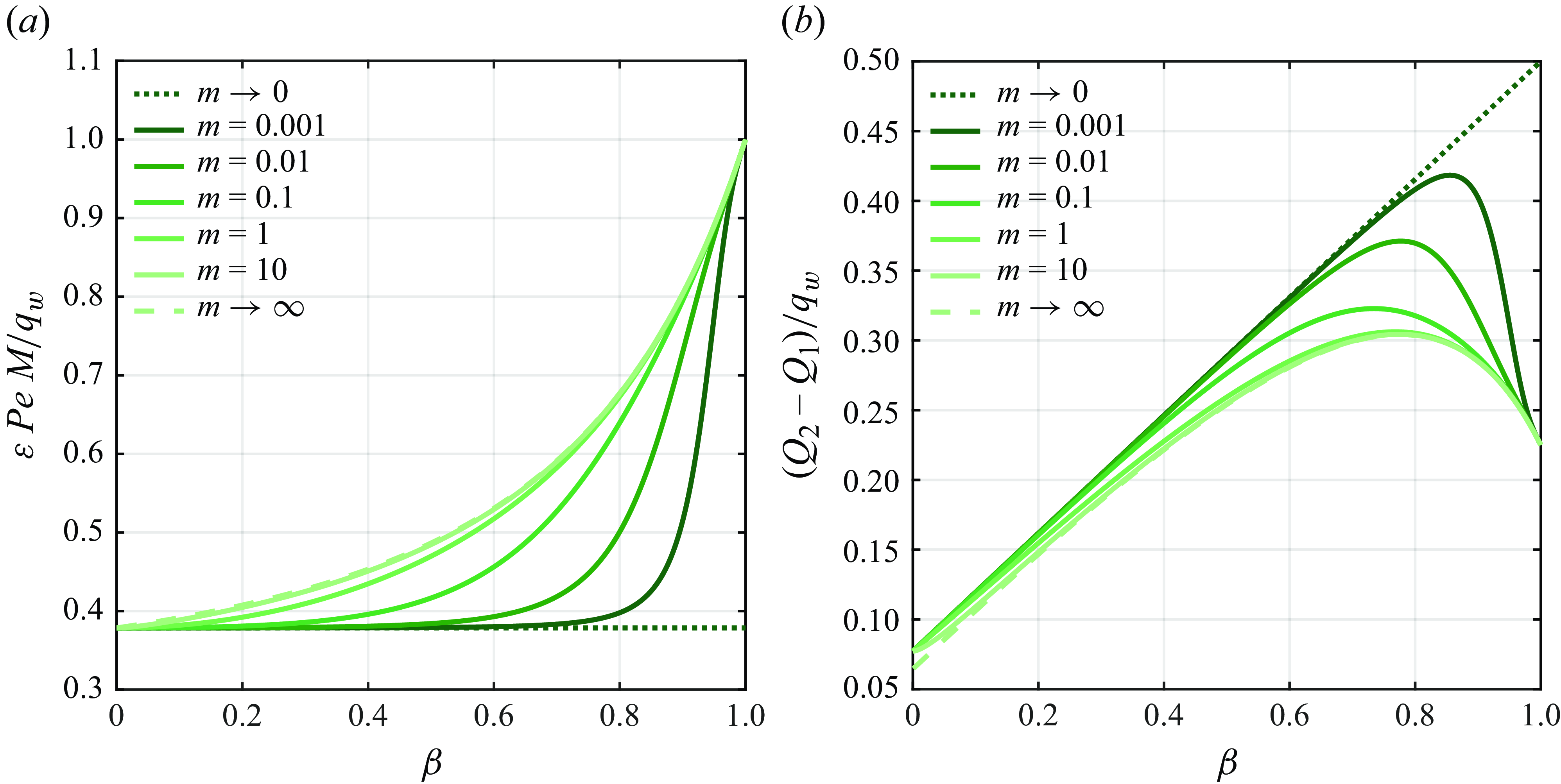
Figure 13. Normalised (a) slope and (b) difference in intercepts for the steady-state solutions (4.21) to the coupled model, as a function of the volume fraction of the outer phase $\beta$
and for fixed values of the viscosity ratio
$\beta$
and for fixed values of the viscosity ratio $m$
, corresponding to a liquid–liquid scenario with
$m$
, corresponding to a liquid–liquid scenario with $\mathcal{A} = 0.51$
and
$\mathcal{A} = 0.51$
and $\mathcal{K} = 5.18$
, see table 1.
$\mathcal{K} = 5.18$
, see table 1.
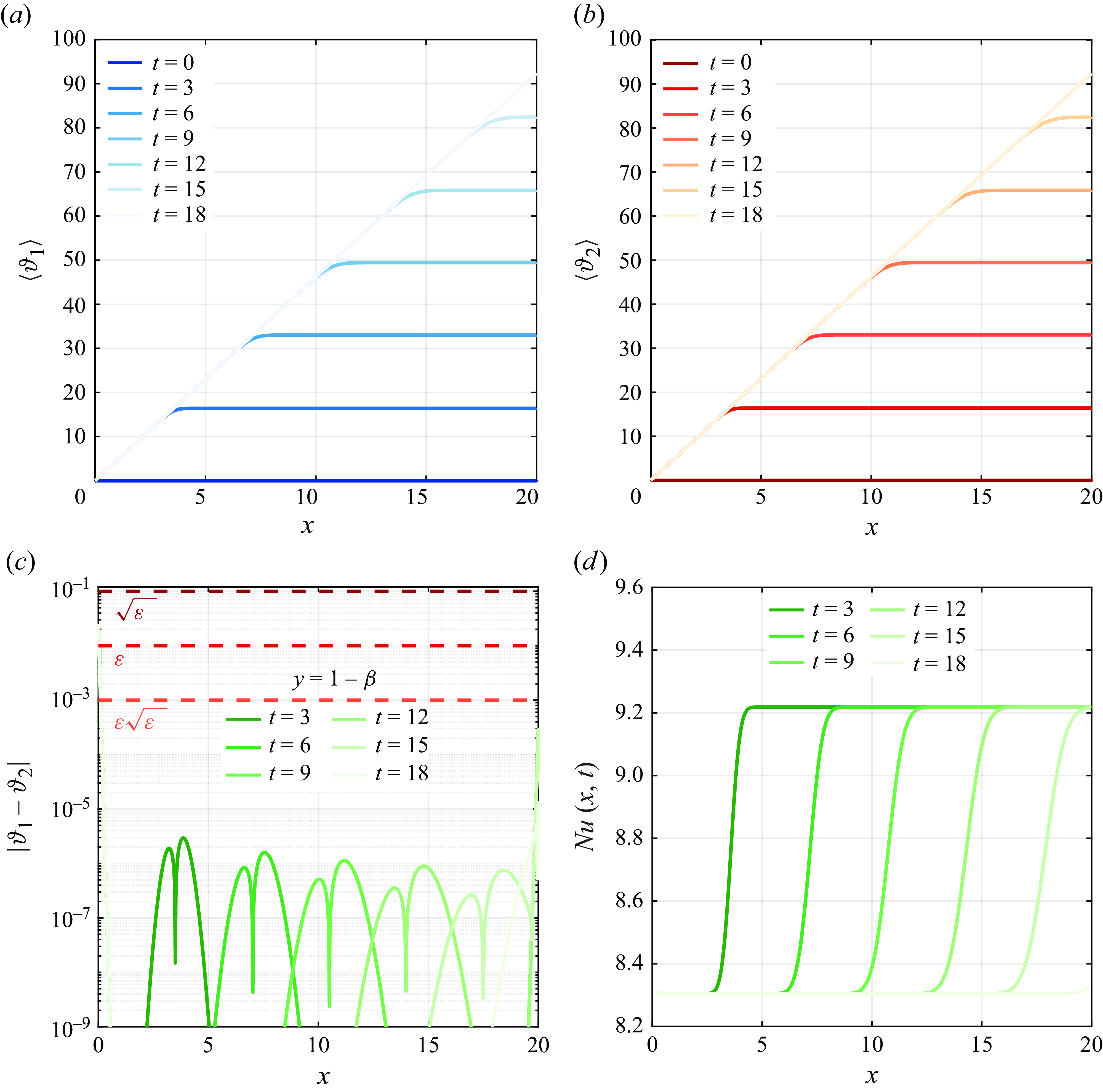
Figure 14. Transient evolution of the averaged temperature $\langle \vartheta _{j}\rangle (x,\,t)$
in the coupled regime, (a)
$\langle \vartheta _{j}\rangle (x,\,t)$
in the coupled regime, (a) $j=1$
, (b)
$j=1$
, (b) $j=2$
. (c) Absolute value of the difference between the temperatures of the two phases at the interface
$j=2$
. (c) Absolute value of the difference between the temperatures of the two phases at the interface $\vartheta _{j}|_{y=1-\beta }$
, including corrections up to the second order. Dashed horizontal lines represent the
$\vartheta _{j}|_{y=1-\beta }$
, including corrections up to the second order. Dashed horizontal lines represent the $\mathcal{O}(\varepsilon ^{1/2},\,\varepsilon, \varepsilon ^{3/2})$
tolerances choosing
$\mathcal{O}(\varepsilon ^{1/2},\,\varepsilon, \varepsilon ^{3/2})$
tolerances choosing $\varepsilon =0.01$
. (d) Time evolution of the Nusselt number
$\varepsilon =0.01$
. (d) Time evolution of the Nusselt number $\boldsymbol{Nu}(x,\,t)$
against the axial coordinate
$\boldsymbol{Nu}(x,\,t)$
against the axial coordinate $x$
. For this liquid–liquid scenario (see table 1), the simulation parameters are:
$x$
. For this liquid–liquid scenario (see table 1), the simulation parameters are: $\boldsymbol{Pe}=1$
,
$\boldsymbol{Pe}=1$
, $\mathcal{A}=0.51$
,
$\mathcal{A}=0.51$
, $\mathcal{K}=5.18$
,
$\mathcal{K}=5.18$
, $m=0.625$
,
$m=0.625$
, $q_{w}=0.1$
,
$q_{w}=0.1$
, $\beta =0.5$
,
$\beta =0.5$
, $\textit{Br}^{\prime }=0$
. Mesh resolution:
$\textit{Br}^{\prime }=0$
. Mesh resolution: $\Delta {x}=0.02$
.
$\Delta {x}=0.02$
.
The transient formulation of (3.8), (3.9) can be solved numerically, as shown in figure 14(a, b), choosing a liquid–liquid system from table 1; the numerical solution has been obtained using the pdepe solver of MATLAB, setting an initial temperature equal to zero in both phases and imposing the steady-state heat flux $M$
, given in (4.22), at the right boundary of the domain (
$M$
, given in (4.22), at the right boundary of the domain ( $x=20$
). A second-order accurate spatial discretisation scheme is employed to convert the original problem into a set of ODEs, which are then integrated to obtain approximate solutions at the specified times (Skeel & Berzins Reference Skeel and Berzins1990). Time discretisation is performed using a multistep variable-step variable-order (VSVO) solver based on numerical differentiation formulae (NDFs) of orders 1–5 (Shampine & Reichelt Reference Shampine and Reichelt1997; Shampine, Reichelt & Kierzenka Reference Shampine, Reichelt and Kierzenka1999). We use equally spaced meshes in the intervals
$x=20$
). A second-order accurate spatial discretisation scheme is employed to convert the original problem into a set of ODEs, which are then integrated to obtain approximate solutions at the specified times (Skeel & Berzins Reference Skeel and Berzins1990). Time discretisation is performed using a multistep variable-step variable-order (VSVO) solver based on numerical differentiation formulae (NDFs) of orders 1–5 (Shampine & Reichelt Reference Shampine and Reichelt1997; Shampine, Reichelt & Kierzenka Reference Shampine, Reichelt and Kierzenka1999). We use equally spaced meshes in the intervals $0\leqslant {x}\leqslant 20$
and
$0\leqslant {x}\leqslant 20$
and $0\leqslant {t}\leqslant 18$
, with 1001 and 501 points, respectively. To ensure highly accurate results, the relative and absolute errors at each integration step have been set to
$0\leqslant {t}\leqslant 18$
, with 1001 and 501 points, respectively. To ensure highly accurate results, the relative and absolute errors at each integration step have been set to $10^{-12}$
, with norm control enabled to manage the overall error in the solution vector. As time elapses, the solution evolves and an increasing region of the channel reaches the steady state.
$10^{-12}$
, with norm control enabled to manage the overall error in the solution vector. As time elapses, the solution evolves and an increasing region of the channel reaches the steady state.
Interestingly, we can use the numerical solution to check the model consistency and verify that the continuity of temperature at the fluid–fluid interface has been properly enforced. This issue represents a key aspect of the model, since such a boundary condition has been imposed in asymptotic terms, see § C.5.2. From figure 14(c), we can see that the temperature difference, $\vartheta _{1}-\vartheta _{2}= (\left \langle \vartheta _{1}\right \rangle +\sqrt {\varepsilon }\,\vartheta _{1}^{(1)}+\varepsilon \,\vartheta _{1}^{(2)} )- (\left \langle \vartheta _{2}\right \rangle +\sqrt {\varepsilon }\,\vartheta _{2}^{(1)}+\varepsilon \,\vartheta _{2}^{(2)} )$
evaluated at the interface and keeping the first three terms of the expansions is within the
$\vartheta _{1}-\vartheta _{2}= (\left \langle \vartheta _{1}\right \rangle +\sqrt {\varepsilon }\,\vartheta _{1}^{(1)}+\varepsilon \,\vartheta _{1}^{(2)} )- (\left \langle \vartheta _{2}\right \rangle +\sqrt {\varepsilon }\,\vartheta _{2}^{(1)}+\varepsilon \,\vartheta _{2}^{(2)} )$
evaluated at the interface and keeping the first three terms of the expansions is within the $\mathcal{O}(\varepsilon \sqrt {\varepsilon })$
error, consistent with the two-scale asymptotic expansion in (3.3). Our model is in fact accurate up to the order
$\mathcal{O}(\varepsilon \sqrt {\varepsilon })$
error, consistent with the two-scale asymptotic expansion in (3.3). Our model is in fact accurate up to the order $\mathcal{O}(\varepsilon )$
.
$\mathcal{O}(\varepsilon )$
.
4.7. Nusselt number in the coupled regime
In the coupled regime, the bulk temperature $\vartheta _{b}$
, see (3.15), simplifies to
$\vartheta _{b}$
, see (3.15), simplifies to
 \begin{equation} \vartheta _{b}\left (x,\,t\right )=\frac {\mathcal{K}\,\mathcal{A}\left (1-\beta \right )U_{1}\left (\left \langle \vartheta _{1}\right \rangle +\sqrt {\varepsilon }\,\vartheta _{1}^{(1)}\right )+\beta \,U_{2}\left (\left \langle \vartheta _{2}\right \rangle +\sqrt {\varepsilon }\,\vartheta _{2}^{(1)}\right )}{\mathcal{K}\,\mathcal{A}\left (1-\beta \right )U_{1}+\beta \,U_{2}} +\mathcal{O}(\varepsilon ), \end{equation}
and the Nusselt number can be computed though the definition (3.19), using the numerical solution of (3.8), (3.9) for the averaged temperatures $\left \langle \vartheta _{j}\right \rangle$
to estimate the first-order terms in (4.24) via (C12) and (C15). The Nusselt number in laminar coupled core-annular flows with uniform wall heat-flux is a function only of
$\left \langle \vartheta _{j}\right \rangle$
to estimate the first-order terms in (4.24) via (C12) and (C15). The Nusselt number in laminar coupled core-annular flows with uniform wall heat-flux is a function only of ${\textit{Nu}}={\textit{Nu}} (x,\,t,\,\beta, \,m,\,\mathcal{A},\,\mathcal{K},\,q_{w},\,{Br}^{\prime },\,{\textit{Pe}} )$
and, based on the definition of the heat-transfer coefficient, see (3.12), it allows for obtaining the two-phase heat-transfer coefficient.
${\textit{Nu}}={\textit{Nu}} (x,\,t,\,\beta, \,m,\,\mathcal{A},\,\mathcal{K},\,q_{w},\,{Br}^{\prime },\,{\textit{Pe}} )$
and, based on the definition of the heat-transfer coefficient, see (3.12), it allows for obtaining the two-phase heat-transfer coefficient.
An example of the time and spatial evolution of ${\textit{Nu}} (x,\,t )$
is given in figure 14(d): the Nusselt number evolves according to an S-shaped trend and is bounded between a lower and an upper horizontal asymptote, corresponding respectively to its limiting values for
${\textit{Nu}} (x,\,t )$
is given in figure 14(d): the Nusselt number evolves according to an S-shaped trend and is bounded between a lower and an upper horizontal asymptote, corresponding respectively to its limiting values for $t\to \infty$
and
$t\to \infty$
and $t\to 0$
. The impact of the Péclet number (i.e. the competition between advection and diffusion) is qualitatively similar to what is described in figure 5(b–f) for the decoupled regime and it is not shown here only for the sake of brevity.
$t\to 0$
. The impact of the Péclet number (i.e. the competition between advection and diffusion) is qualitatively similar to what is described in figure 5(b–f) for the decoupled regime and it is not shown here only for the sake of brevity.
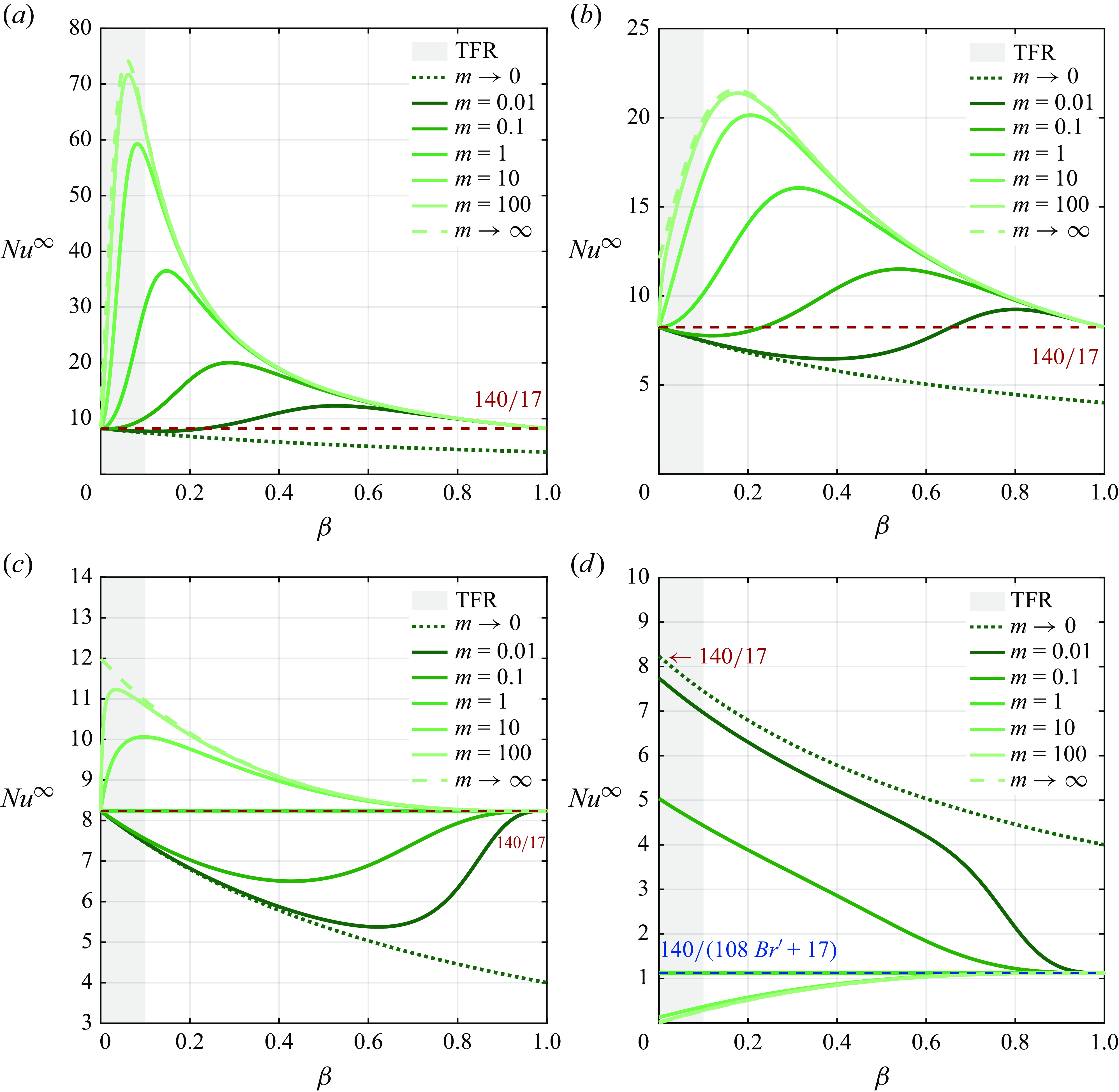
Figure 15. Limiting two-phase Nusselt number for a core-annular flow of unitary conductivity ratio, $\mathcal{K}=1$
, as a function of the volume fraction
$\mathcal{K}=1$
, as a function of the volume fraction $\beta$
, for fixed values of the viscosity ratio
$\beta$
, for fixed values of the viscosity ratio $m$
. Panels (a) to (c) refer to a non-dissipative core-annular flow (
$m$
. Panels (a) to (c) refer to a non-dissipative core-annular flow ( ${Br}^{\prime }=0$
) with increasing diffusivity ratios as increasing powers of the small-scale parameter,
${Br}^{\prime }=0$
) with increasing diffusivity ratios as increasing powers of the small-scale parameter, $\varepsilon =0.01$
: (a)
$\varepsilon =0.01$
: (a) $\mathcal{A}=\varepsilon$
, (b)
$\mathcal{A}=\varepsilon$
, (b) $\mathcal{A}=\sqrt {\varepsilon }$
, (c)
$\mathcal{A}=\sqrt {\varepsilon }$
, (c) $\mathcal{A}=1$
. In (d),
$\mathcal{A}=1$
. In (d), $\mathcal{A}={Br}^{\prime }=1$
.
$\mathcal{A}={Br}^{\prime }=1$
.
At the steady state, the axial gradients of temperature $\partial \langle \vartheta _{j}\rangle /\partial x$
can be replaced by the slope
$\partial \langle \vartheta _{j}\rangle /\partial x$
can be replaced by the slope $M$
given in (4.21) and the Nusselt number
$M$
given in (4.21) and the Nusselt number $ {\textit{Nu}}^{\infty }= {\textit{Nu}}^{\infty } (\beta, m, \mathcal{A}, \mathcal{K}, {Br}^{\prime } )$
can be written in a closed form (its full expression looks quite cumbersome and it is not reported here only for the sake of brevity). Figure 15 shows the evolution of
$ {\textit{Nu}}^{\infty }= {\textit{Nu}}^{\infty } (\beta, m, \mathcal{A}, \mathcal{K}, {Br}^{\prime } )$
can be written in a closed form (its full expression looks quite cumbersome and it is not reported here only for the sake of brevity). Figure 15 shows the evolution of $ {\textit{Nu}}^{\infty }$
with respect to the volume fraction and the viscosity ratio for a liquid–liquid case, see table 1, keeping the conductivity ratio as
$ {\textit{Nu}}^{\infty }$
with respect to the volume fraction and the viscosity ratio for a liquid–liquid case, see table 1, keeping the conductivity ratio as $\mathcal{K}=1$
; the panels (
$\mathcal{K}=1$
; the panels ( $a$
)–(
$a$
)–( $c$
) show the effect of the diffusivity ratio
$c$
) show the effect of the diffusivity ratio $\mathcal{A}$
. First, the single-phase limits of the steady-state Nusselt number for a vanishing core (i.e. the channel section is entirely occupied by the outer phase) yields to
$\mathcal{A}$
. First, the single-phase limits of the steady-state Nusselt number for a vanishing core (i.e. the channel section is entirely occupied by the outer phase) yields to
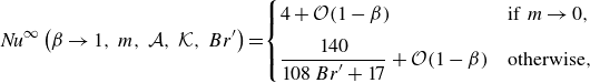 \begin{equation} {\textit{Nu}}^{\infty }\left (\beta \to 1,\,m,\,\mathcal{A},\,\mathcal{K},\,{Br}^{\prime }\right )=\! \begin{cases} 4 + \mathcal{O}(1-\beta )& \text{if}\,\, m \to 0,\\[6pt] \dfrac {140}{108\,{Br}^{\prime }+17} + \mathcal{O}(1-\beta ) & \text{otherwise}, \end{cases} \end{equation}
confirming that the result obtained as $m\not \to 0$
is consistent with the single-phase benchmark expression given by (278) of Shah & London (Reference Shah and London1978) (
$m\not \to 0$
is consistent with the single-phase benchmark expression given by (278) of Shah & London (Reference Shah and London1978) ( ${\textit{Nu}}^{\infty }=140/17$
) for a uniform heat flux boundary condition imposed in a planar channel. Note that in the free-surface limit,
${\textit{Nu}}^{\infty }=140/17$
) for a uniform heat flux boundary condition imposed in a planar channel. Note that in the free-surface limit, $m\to 0$
, the outer phase moves so slowly (see figure 3
d) that the heat flux cannot be convected downstream and the Nusselt number converges to the value of
$m\to 0$
, the outer phase moves so slowly (see figure 3
d) that the heat flux cannot be convected downstream and the Nusselt number converges to the value of $4$
, in agreement with the case of two different temperatures specified at each boundary, see (268) of Shah & London (Reference Shah and London1978).
$4$
, in agreement with the case of two different temperatures specified at each boundary, see (268) of Shah & London (Reference Shah and London1978).
Interestingly, when $m\to 0$
, the convective heat-transfer is less efficient compared with the single-phase flow and
$m\to 0$
, the convective heat-transfer is less efficient compared with the single-phase flow and ${\textit{Nu}}^{\infty }\lt 140/17$
in the whole range of volume fractions, see figure 15(a–c). In the free-surface limit, in fact, the annulus moves so slowly (see figure 3
c) that the asymptotic Nusselt number is unaffected by the thermal diffusivity ratio
${\textit{Nu}}^{\infty }\lt 140/17$
in the whole range of volume fractions, see figure 15(a–c). In the free-surface limit, in fact, the annulus moves so slowly (see figure 3
c) that the asymptotic Nusselt number is unaffected by the thermal diffusivity ratio $\mathcal{A}$
:
$\mathcal{A}$
:
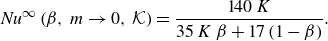 \begin{equation} {\textit{Nu}}^{\infty }\left (\beta, \,m\to 0,\,\mathcal{K}\right )=\frac {140\,K}{35\,K\,\beta +17\left (1-\beta \right )}. \end{equation}
Notice that, in the coupled regime ( $k=0$
), the use of
$k=0$
), the use of $K$
or
$K$
or $\mathcal{K}=K\,\varepsilon ^{k}$
is equivalent in (4.26). In the rigid core limit, instead, convective heat-transfer is favoured and is always enhanced compared with the single-phase flow, namely
$\mathcal{K}=K\,\varepsilon ^{k}$
is equivalent in (4.26). In the rigid core limit, instead, convective heat-transfer is favoured and is always enhanced compared with the single-phase flow, namely ${\textit{Nu}}^{\infty }\gt 140/17$
, in the whole range of
${\textit{Nu}}^{\infty }\gt 140/17$
, in the whole range of $\beta$
. This can be explained by the shape of the velocity profile (linear in the annulus and flat in the core, see figure 3
c), that maximises heat transfer ensuring the most efficient replacement of fluid over the heated surface. This effect is amplified by lowering the diffusivity ratio
$\beta$
. This can be explained by the shape of the velocity profile (linear in the annulus and flat in the core, see figure 3
c), that maximises heat transfer ensuring the most efficient replacement of fluid over the heated surface. This effect is amplified by lowering the diffusivity ratio $\mathcal{A}$
. Specifically, the thermal diffusivity represents the promptness of a material in dissipating a temperature inhomogeneity relative to its tendency to store thermal energy, and, therefore, when
$\mathcal{A}$
. Specifically, the thermal diffusivity represents the promptness of a material in dissipating a temperature inhomogeneity relative to its tendency to store thermal energy, and, therefore, when $\mathcal{A}$
is less than one, the diffusivity of the core is greater than that of the annulus. In our case, a lower value of
$\mathcal{A}$
is less than one, the diffusivity of the core is greater than that of the annulus. In our case, a lower value of $\mathcal{A}$
results in a greater tendancy of the outer phase to accumulate the heat received from the surroundings rather than diffusing it, enhancing the heat-transfer coefficient. This behaviour is favoured at low volume fractions, i.e. when the fluid in contact with the channel wall is sufficiently thin. In contrast, increasing
$\mathcal{A}$
results in a greater tendancy of the outer phase to accumulate the heat received from the surroundings rather than diffusing it, enhancing the heat-transfer coefficient. This behaviour is favoured at low volume fractions, i.e. when the fluid in contact with the channel wall is sufficiently thin. In contrast, increasing $\beta$
leads to a larger thermal resistance in the annulus and gives a greater difference between the wall and the bulk temperature defined in (4.24), reducing the heat-transfer coefficient
$\beta$
leads to a larger thermal resistance in the annulus and gives a greater difference between the wall and the bulk temperature defined in (4.24), reducing the heat-transfer coefficient $h$
and the Nusselt number.
$h$
and the Nusselt number.
In other words, two-phase flows enhance convective heat transfer only under certain conditions. Specifically, only if the viscosity ratio is finite and the diffusivity ratio is small enough, we observe an enhanced heat-transfer coefficient, in particular at low volume fractions.
Finally, the effect of viscous dissipation on the Nusselt number is shown in figure 15(d), setting ${Br}^{\prime }=1$
while keeping
${Br}^{\prime }=1$
while keeping $\mathcal{A}=1$
. When the two fluids have the same viscosity, i.e.
$\mathcal{A}=1$
. When the two fluids have the same viscosity, i.e. $m=1$
, the Nusselt number does not depend on the volume fraction and viscous dissipation lowers the value of
$m=1$
, the Nusselt number does not depend on the volume fraction and viscous dissipation lowers the value of $140/(108\,{Br}^{\prime }+17)$
. The curves obtained for values of
$140/(108\,{Br}^{\prime }+17)$
. The curves obtained for values of $m$
larger than
$m$
larger than $1$
are located below this threshold, while those where
$1$
are located below this threshold, while those where $0\lt m\lt 1$
lie above it. In any case, viscous heating (
$0\lt m\lt 1$
lie above it. In any case, viscous heating ( ${Br}^{\prime }\gt 0$
) reduces the efficiency of convective heat-transfer and the dependence on the viscosity ratio is flipped compared with the non-dissipative scenario. This can be attributed to the combination of two factors (Shah & London Reference Shah and London1978): (i) a reduction in the wall temperature gradient near the wall region due to viscous heating; and (ii) a slower rise of the bulk temperature along the channel axis, due to a reduced amount of heat transferred through the wall.
${Br}^{\prime }\gt 0$
) reduces the efficiency of convective heat-transfer and the dependence on the viscosity ratio is flipped compared with the non-dissipative scenario. This can be attributed to the combination of two factors (Shah & London Reference Shah and London1978): (i) a reduction in the wall temperature gradient near the wall region due to viscous heating; and (ii) a slower rise of the bulk temperature along the channel axis, due to a reduced amount of heat transferred through the wall.
5. Conclusions
Forced convection in two-phase channel flows arises in a large variety of applications. In this paper, we derived an asymptotic one-dimensional model to describe the heat transfer in laminar core-annular flows in a planar geometry heated by a uniform heat-flux (extended Graetz-type problem).
The main heat-transfer mechanisms (advection and diffusion) occurring along the transversal and the longitudinal direction has been modelled via effective coefficients, which depend on the Péclet and Brinkman numbers, the dimensionless heat flux, the viscosity, thermal diffusivity and thermal conductivity ratios, and the volume fraction only. Specifically, the resulting diffusion coefficients provide a generalisation of the classical Aris–Taylor dispersion theory to two-phase flows. The model reveals the existence of two main regimes, depending on the thermal capacity of the two phases.
When the thermal conductivities of the two fluids are of the same order of magnitude, as in liquid–liquid systems, the system is described by two-coupled advection–diffusion heat-transfer equations. The coupling between the phases results in a canonical and a coupled effective advection term, a canonical and a cross-coupling effective diffusion term, and storage and source terms for each phase. We derived an analytical model for the Nusselt number revealing that the heat transfer is enhanced with respect to the single-phase scenario only if the viscosity ratio is finite and the diffusivity ratio is small enough. In addition to that, we identified the dominant regime controlling thermal mixing depending on the magnitude of the Péclet number. In particular, at small ${\textit{Pe}}$
, the transport of thermal energy is dominated by diffusion. For intermediate values of the Péclet number, advection and diffusion compete, leading to a strong influence of both the flow condition (i.e. Péclet number) and the properties of the system (i.e. volume fraction, viscosity, thermal conductivity and thermal diffusivity ratios) on the dispersion coefficient. At high
${\textit{Pe}}$
, the transport of thermal energy is dominated by diffusion. For intermediate values of the Péclet number, advection and diffusion compete, leading to a strong influence of both the flow condition (i.e. Péclet number) and the properties of the system (i.e. volume fraction, viscosity, thermal conductivity and thermal diffusivity ratios) on the dispersion coefficient. At high ${\textit{Pe}}$
, heat transport is fully dominated by advection.
${\textit{Pe}}$
, heat transport is fully dominated by advection.
When the annulus is more conductive than the core, as in most liquid–gas systems, the phases are thermally decoupled and the averaged temperature of the core evolves according to a single one-dimensional advection–diffusion heat-transfer equation. In this case, the limiting Nusselt number scales as the inverse of the annulus thickness and it is independent of the viscosity ratio. If the annulus is thin, our model confirms that, within the film, the heat-transfer is primarily driven by conduction and the temperature profile remains almost linear along the transverse direction. Interestingly, in the advection-dominated regime, the core-annular flow pattern does not enhance thermal mixing compared with single-phase flow, in particular when the volume fraction is small. Our analysis is complemented by the identification of a hierarchy between the characteristic time scales of advection and diffusion, helping in understanding the proper time window where thermal dispersion can be observed.
Our work clarifies the impact of the phases topology on forced convection and we hope that it may be extended with the aim of offering a more rigorous interpretation of the heat-transfer phenomena taking place in more complex two-phase flow patterns.
Funding
This study has received funding from the European Union ‘NextGenerationEU’, Ministero dell’Università e della Ricerca (MUR) ‘Italiadomani’ Piano Nazionale di Ripresa e Resilienza (PNRR), Mission 4, Research Project PRIN 2022 ‘Predictive forecasting and risk assessment for $\textrm {CO}_{2}$
transport in pipelines’, MUR code: 20229JPN53; CUP Master code: J53D23002000006; CUP code: D53D23003250006.
$\textrm {CO}_{2}$
transport in pipelines’, MUR code: 20229JPN53; CUP Master code: J53D23002000006; CUP code: D53D23003250006.
Declaration of interests
The authors report no conflict of interest.
Appendix A. Velocity profiles
Consider a core-annular flow as shown in figure 1 at laminar and steady-state conditions: the system is composed by two immiscible and incompressible fluids with no interfacial instabilities or entrainment of one phase into the other (Joseph, Nguyen & Beavers Reference Joseph, Nguyen and Beavers1984) and in the absence of any body forces (such as buoyancy). The channel is assumed to be shallow enough ( $\hat {H}/\hat {L}\ll 1$
) so that the momentum equations of each phase are simplified using the lubrication approximation and the flow is treated as one-dimensional (the velocity components in the transverse and normal directions are neglected). The momentum equation for each
$\hat {H}/\hat {L}\ll 1$
) so that the momentum equations of each phase are simplified using the lubrication approximation and the flow is treated as one-dimensional (the velocity components in the transverse and normal directions are neglected). The momentum equation for each $j$
th-Newtonian fluid, then, reduces to
$j$
th-Newtonian fluid, then, reduces to
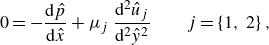 \begin{equation} 0=-\frac {\mathrm{d}\hat {p}}{\mathrm{d}\hat {x}}+\mu _{j}\,\frac {\mathrm{d}^2\hat {u}_{j}}{\mathrm{d}^2\hat {y}^{2}} \quad \quad j=\left \{1,\,2\right \}, \end{equation}
subjected to the following boundary conditions:
 \begin{align} \left .\frac {\mathrm{d}\hat {u}_{1}}{\mathrm{d}\hat {y}}\right |_{\hat {y}=0}&=0, \end{align}
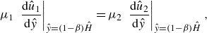 \begin{align} \mu _{1}\,\left .\frac {\mathrm{d}\hat {u}_{1}}{\mathrm{d}\hat {y}}\right |_{\hat {y}=\left (1-\beta \right )\hat {H}}&=\mu _{2}\,\left .\frac {\mathrm{d}\hat {u}_{2}}{\mathrm{d}\hat {y}}\right |_{\hat {y}=\left (1-\beta \right )\hat {H}}, \end{align}
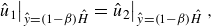 \begin{align} \left .\hat {u}_{1}\right |_{\hat {y}=\left (1-\beta \right )\hat {H}}&=\left .\hat {u}_{2}\right |_{\hat {y}=\left (1-\beta \right )\hat {H}}, \end{align}
 \begin{align} \left .\hat {u}_{2}\right |_{\hat {y}=\hat {H}}&=0, \end{align}
namely, the symmetry of the inner velocity profile with respect to the channel axis (A2a ), the continuity of tangential stresses (A2b ) and velocities (A2c ) at the interface, and, the no-slip condition at the channel wall. The set of equations (A1) admits the following analytical solution
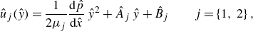 \begin{equation} \hat {u}_{j}(\hat {y})=\frac {1}{2{\mu }_{j}}\frac {\mathrm{d}\hat {p}}{\mathrm{d}\hat {x}}\,\hat {y}^{2}+\hat {A}_{j}\,\hat {y}+\hat {B}_{j} \quad \quad j=\left \{1,\,2\right \}, \end{equation}
where $\hat {A}_{j},\,\hat {B}_{j}$
are constants to be determined imposing the boundary conditions given in (A2):
$\hat {A}_{j},\,\hat {B}_{j}$
are constants to be determined imposing the boundary conditions given in (A2):
 \begin{align} & \hat {A}_{1}=0, &\qquad & \hat {A}_{2}=0, \end{align}
 \begin{align} & \hat {B}_{1}=-\frac {1}{2}\,\frac {\mathrm{d}\hat {p}}{\mathrm{d}\hat {x}}\,\frac {\hat {H}^{2}\left [\mu _{2}-\beta (2-\beta)\left (\mu _{2}-\mu _{1}\right )\right ]}{\mu _{1}\,\mu _{2}}, && \hat {B}_{2}=-\frac {1}{2}\,\frac {\mathrm{d}\hat {p}}{\mathrm{d}\hat {x}}\,\frac {\hat {H}^{2}}{\mu _{2}}, \end{align}
leading to the dimensional velocity fields expressed in (2.1). Effects related to thermo-capillary Marangoni convection have not been considered in this work.
A.1 Dimensionless velocity profiles
The dimensionless velocity profiles $u_{j} (y )$
normalised using (2.12b,d
) are given by
$u_{j} (y )$
normalised using (2.12b,d
) are given by
 \begin{align} & u_{1}(y)=3\,\Lambda [1+\beta (2-\beta )(m-1)-y^2], &\qquad & u_{2}(y)=3\,\Lambda \,m (1-y^2), \end{align}
 \begin{align} & U_{1}=\Lambda [ \vphantom{\beta^{2}}2+\beta (2-\beta)(3m-2)], && U_{2}=\Lambda \,m\beta (3-\beta ), \end{align}
with
 \begin{equation} \Lambda ^{-1}=2[1+\beta (\beta ^2-3\beta +3)(m-1)]. \end{equation}
Figure 3(c) shows the velocity profiles (A5a
) as a function of the viscosity ratio $m$
. When
$m$
. When $m\to \infty$
, the inner fluid approaches the constant plug-like profile and we will refer to it as the rigid-core limit; conversely, the outer velocity profile becomes linear in the free-surface limit when
$m\to \infty$
, the inner fluid approaches the constant plug-like profile and we will refer to it as the rigid-core limit; conversely, the outer velocity profile becomes linear in the free-surface limit when $m\to 0$
(Balestra et al. Reference Balestra, Zhu and Gallaire2018).
$m\to 0$
(Balestra et al. Reference Balestra, Zhu and Gallaire2018).
The evolution of the average speed $U_{j}$
, see (A5b
), against the volume fraction of the outer phase for different values of the viscosity ratio is presented in figure 3(d).
$U_{j}$
, see (A5b
), against the volume fraction of the outer phase for different values of the viscosity ratio is presented in figure 3(d).
Appendix B. Heat capacity flow rate ratio
In Graetz-type heat exchange problems, the heat capacity flow rate ratio (or capacitance ratio) $\text{Cr}$
is widely used. This dimensionless number is the ratio between the heat capacity rates (the product of mass flow rate
$\text{Cr}$
is widely used. This dimensionless number is the ratio between the heat capacity rates (the product of mass flow rate $\dot {m}_{j}$
and specific heat capacity at constant pressure
$\dot {m}_{j}$
and specific heat capacity at constant pressure $c_{p,\,j}$
) of the two phases flowing in a heat exchanger (Bai et al. Reference Bai, Zhu, Chen and Chu2018). For the core-annular configuration depicted in figure 1,
$c_{p,\,j}$
) of the two phases flowing in a heat exchanger (Bai et al. Reference Bai, Zhu, Chen and Chu2018). For the core-annular configuration depicted in figure 1, $\text{Cr}$
is computed combining (2.14c
, A5b
, A6) as
$\text{Cr}$
is computed combining (2.14c
, A5b
, A6) as
 \begin{equation} \text{Cr}=\frac {\dot {m}_{2}\,c_{p,\,2}}{\dot {m}_{1}\,c_{p,\,1}}= \frac {\rho _{2}}{\rho _{1}}\, \frac {\beta }{1-\beta }\, \frac {U_{2}}{U_{1}}\, \frac {c_{p,\,2}}{c_{p,\,1}}= \frac {1}{\mathcal{K}\,\mathcal{A}}\, \frac {\beta ^2\,m(3-\beta )}{\left (1-\beta \right ) \left [2\left (1-\beta \right )^{2}+3\,m\,\beta (2-\beta)\right ]}. \end{equation}
From the physical point of view, the heat capacity ratio governs the distribution of heat between the two phases and plays a crucial role in determining the overall effectiveness of heat transfer. Specifically, $\textrm {Cr}$
describes how efficiently the energy is transferred from one phase to the other: the optimal performance is obtained when
$\textrm {Cr}$
describes how efficiently the energy is transferred from one phase to the other: the optimal performance is obtained when $\text{Cr}\approx 1$
, while for
$\text{Cr}\approx 1$
, while for $\text{Cr}\to 0$
or
$\text{Cr}\to 0$
or $\text{Cr}\to \infty$
, its effectiveness is limited due to one phase dominating the heat transfer process. The
$\text{Cr}\to \infty$
, its effectiveness is limited due to one phase dominating the heat transfer process. The $\text{Cr}$
is typically related to the design and the optimisation of heat exchangers, e.g. the NTU (number of transfer units) method (Langerova & Matuska Reference Langerova and Matuska2023).
$\text{Cr}$
is typically related to the design and the optimisation of heat exchangers, e.g. the NTU (number of transfer units) method (Langerova & Matuska Reference Langerova and Matuska2023).
In figure 16, we plot the capacitance ratio against the volume fraction of the outer phase for different values of the viscosity ratio for liquid–liquid and gas–liquid systems, identified by the order of magnitude of the thermal capacity ratio (i.e. the product $\mathcal{K}\,\mathcal{A}$
). Referring to table 1, we can assume that
$\mathcal{K}\,\mathcal{A}$
). Referring to table 1, we can assume that $\mathcal{K}\,\mathcal{A}\approx 1$
in liquid–liquid and
$\mathcal{K}\,\mathcal{A}\approx 1$
in liquid–liquid and $\mathcal{K}\,\mathcal{A}\approx 10^{-3}$
for gas–liquid systems. Interestingly,
$\mathcal{K}\,\mathcal{A}\approx 10^{-3}$
for gas–liquid systems. Interestingly, $\text{Cr}$
increases with
$\text{Cr}$
increases with $m$
while keeping
$m$
while keeping $\beta$
fixed for both liquid–liquid and gas–liquid systems, and the optimal condition of
$\beta$
fixed for both liquid–liquid and gas–liquid systems, and the optimal condition of $\textrm {Cr}=1$
shifts to lower
$\textrm {Cr}=1$
shifts to lower $\beta$
, see figure 16.
$\beta$
, see figure 16.
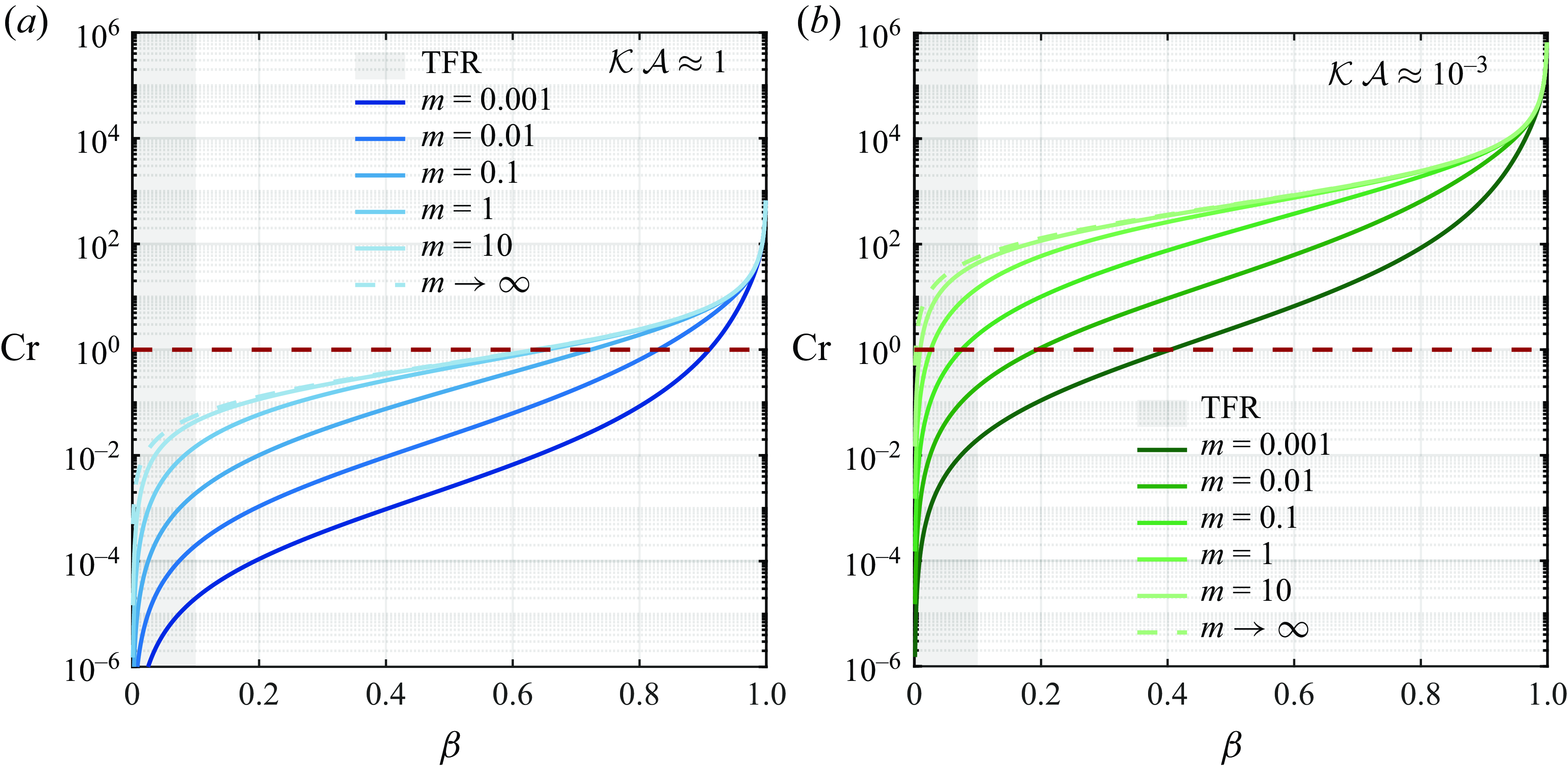
Figure 16. Evolution of the heat capacity flow rate ratio $\text{Cr}$
as a function of the dimensionless thickness of the outer layer
$\text{Cr}$
as a function of the dimensionless thickness of the outer layer $\beta$
for different values of the viscosity ratio
$\beta$
for different values of the viscosity ratio $m$
in (a) liquid–liquid and (b) gas–liquid systems. The two set of curves differ for the thermal capacity ratio
$m$
in (a) liquid–liquid and (b) gas–liquid systems. The two set of curves differ for the thermal capacity ratio $\mathcal{K}\,\mathcal{A}$
. The TFR is highlighted by the grey area.
$\mathcal{K}\,\mathcal{A}$
. The TFR is highlighted by the grey area.
Appendix C. Derivation of the heat-transfer model using two-scale asymptotic expansion
In the following sections, the derivation of the effective equations is carried out following the procedure discussed in § 3.
C.1 Expanded governing equations
After making the axial-coordinate stretching (3.1) and using (3.2), the governing equations (2.13) become
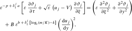 \begin{eqnarray} && \varepsilon ^{-p\,+\,\delta _{1}^{j}\,a}\left [\varepsilon \,\frac {\partial \vartheta _{j}}{\partial \tau }+\sqrt {\varepsilon }\,\left (u_{j}-V\right )\frac {\partial \vartheta _{j}}{\partial \xi }\right ] = \left (\varepsilon \,\frac {\partial ^{2} \vartheta _{j}}{\partial \xi ^{2}}+\frac {\partial ^{2} \vartheta _{j}}{\partial y^{2}}\right ) \nonumber\\&&\quad +\, B\,\varepsilon ^{b\,+\,\delta _{1}^{j}\,\left [ \log _{\varepsilon }\!{\left ({m}/{K}\right )-k}\right ] } \left (\frac {\mathrm{d}{u}_{j}}{\mathrm{d}{y}}\right )^{\!2}\!\!, \end{eqnarray}
where $u_{j} (y )$
is the velocity profile of the
$u_{j} (y )$
is the velocity profile of the $j$
-phase given in (A5),
$j$
-phase given in (A5), $V$
is the velocity of the moving reference frame, and
$V$
is the velocity of the moving reference frame, and $\delta ^{j}_{1}=1-\delta ^{j}_{2}$
is the Kronecker delta defined in (3.7) and introduced to make the model derivation more compact. Plugging the expansion (3.3) into (C1) leads to
$\delta ^{j}_{1}=1-\delta ^{j}_{2}$
is the Kronecker delta defined in (3.7) and introduced to make the model derivation more compact. Plugging the expansion (3.3) into (C1) leads to
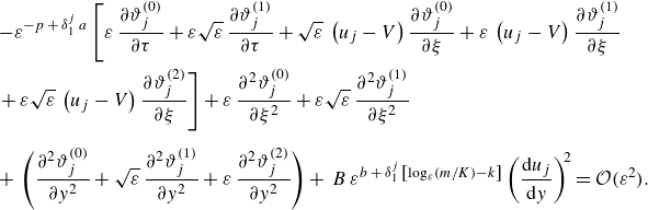 \begin{eqnarray} && -\varepsilon ^{-p\,+\,\delta _{1}^{j}\,a} \left [\varepsilon \,\frac {\partial \vartheta _{j}^{(0)}}{\partial \tau }+ \varepsilon \sqrt {\varepsilon }\,\frac {\partial \vartheta _{j}^{(1)}}{\partial \tau }+ \sqrt {\varepsilon }\,\left (u_{j}-V\right )\frac {\partial \vartheta _{j}^{(0)}}{\partial \xi }+ \varepsilon \,\left (u_{j}-V\right )\frac {\partial \vartheta _{j}^{(1)}}{\partial \xi} \right. \nonumber \\[0pt] && \left. +\, \varepsilon \sqrt {\varepsilon }\,\left (u_{j}-V\right )\frac {\partial \vartheta _{j}^{(2)}}{\partial \xi } \right ] +\varepsilon \,\frac {\partial ^{2} \vartheta _{j}^{(0)}}{\partial \xi ^{2}} +\varepsilon \sqrt {\varepsilon }\,\frac {\partial ^{2} \vartheta _{j}^{(1)}}{\partial \xi ^{2}}\nonumber \\[6pt]&& +\, \left (\frac {\partial ^{2} \vartheta _{j}^{(0)}}{\partial y^{2}}+ \sqrt {\varepsilon }\,\frac {\partial ^{2} \vartheta _{j}^{(1)}}{\partial y^{2}}+ \varepsilon \,\frac {\partial ^{2} \vartheta _{j}^{(2)}}{\partial y^{2}} \right ) +\, B\,\varepsilon ^{b\,+\,\delta _{1}^{j}\,\left [ \log _{\varepsilon }\!{\left ({m}/{K}\right )-k}\right ] } \left (\frac {\mathrm{d}{u}_{j}}{\mathrm{d}{y}}\right )^{\!2} = \mathcal{O}(\varepsilon ^{2}). \nonumber\\ \end{eqnarray}
Since the employed asymptotic expansion (3.3) was truncated to its first three terms, a cascade of equations for the unknown functions $\vartheta _{j}^{(n)}$
, with
$\vartheta _{j}^{(n)}$
, with $n=\{0,\,1,\,2\}$
, originates from (C2). Specifically, we obtain
$n=\{0,\,1,\,2\}$
, originates from (C2). Specifically, we obtain
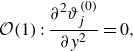 \begin{align} \mathcal{O}(1): \def\lumina\hspace {0.05cm}\frac {\partial ^2 \vartheta _{j}^{(0)}}{\partial y^2}=0\,\!, \end{align}
 \begin{align} \mathcal{O}(\sqrt {\varepsilon }): \def\lumina\hspace {0.05cm} \frac {\partial ^2 \vartheta _{j}^{(1)}}{\partial y^2}= \varepsilon ^{-p\,+\,\delta _{1}^{j}\,a} \left ({u}_{j} - V\right )\frac {\partial \vartheta _{j}^{(0)}}{\partial \xi } - B\,\varepsilon ^{b\,-\,\frac {1}{2}\,+\,\delta _{1}^{j}\,\left [ \log _{\varepsilon }\!{\left (\frac {m}{K}\right )-k}\right ] }\left (\frac {\mathrm{d}{u}_{j}}{\mathrm{d}{y}}\right )^{\!\!2}\!, \end{align}
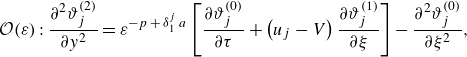 \begin{align} \mathcal{O}(\varepsilon ): \def\lumina\hspace {0.05cm} \frac {\partial ^2 \vartheta _{j}^{(2)}}{\partial y^2}= \varepsilon ^{-p\,+\,\delta _{1}^{j}\,a} \left [\frac {\partial \vartheta _{j}^{(0)}}{\partial \tau } + \left ({u}_{j} - V\right ) \frac {\partial \vartheta _{j}^{(1)}}{\partial \xi } \right ]-\frac {\partial ^2 \vartheta _{j}^{(0)}}{\partial \xi ^2}, \end{align}
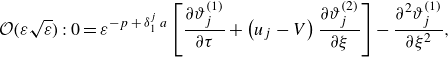 \begin{align} \mathcal{O}(\varepsilon \sqrt {\varepsilon }): \def\lumina\hspace {0.05cm}\def\lumina\hspace {0.45cm} 0\def\lumina\hspace {0.4cm}= \varepsilon ^{-p\,+\,\delta _{1}^{j}\,a} \left [\frac {\partial \vartheta _{j}^{(1)}}{\partial \tau } + \left ({u}_{j} - V\right ) \frac {\partial \vartheta _{j}^{(2)}}{\partial \xi } \right ]-\frac {\partial ^2 \vartheta _{j}^{(1)}}{\partial \xi ^2}, \end{align}
where the order of magnitude of the governing parameters is within the applicability region discussed in § 3.1 and has been chosen in a way that ensures the least degeneracy of the closure problem (Van Dyke Reference Van Dyke1964). In other words, we keep the maximum possible number of non-vanishing small terms (Feuillebois & Lasek Reference Feuillebois and Lasek1977) when equal powers of $\varepsilon$
are gathered from the expanded governing equation (C2). Doing so, all the relevant physical effects enter the problem as soon as practicable and not beyond (Richard et al. Reference Richard, Ruyer-Quil and Vila2016).
$\varepsilon$
are gathered from the expanded governing equation (C2). Doing so, all the relevant physical effects enter the problem as soon as practicable and not beyond (Richard et al. Reference Richard, Ruyer-Quil and Vila2016).
C.1.1 Boundary conditions
The boundary conditions (2.16) have to be expanded so that at each order in (C3), we obtain a boundary-value problem in the form of a second-order linear partial differential equation (PDE) that can be solved integrating twice in $y$
.
$y$
.
The continuity of thermal fluxes across the interface (2.16b ) reads
 \begin{align} \left .\left (\frac {\partial \vartheta _{2}^{(0)}}{\partial y} +\sqrt {\varepsilon }\frac {\partial \vartheta _{2}^{(1)}}{\partial y} +\varepsilon \frac {\partial \vartheta _{2}^{(2)}}{\partial y} \right )\right |_{y=1-\beta }= \,\mathcal{K}\left .\left (\frac {\partial \vartheta _{1}^{(0)}}{\partial y} +\sqrt {\varepsilon }\frac {\partial \vartheta _{1}^{(1)}}{\partial y} +\varepsilon \frac {\partial \vartheta _{1}^{(2)}}{\partial y} \right )\right |_{y=1-\beta },\nonumber\\[-2pt] \end{align}
suggesting the identification of several regimes based on the order of magnitude of the thermal conductivity ratio $\mathcal{K}$
. In this work, we will focus on regimes where the inner phase exhibits a comparable (
$\mathcal{K}$
. In this work, we will focus on regimes where the inner phase exhibits a comparable ( $k=0$
) or lower (
$k=0$
) or lower ( $k\gt 0$
) thermal conductivity with respect to that of the outer phase only. Therefore, depending on the order of magnitude of the conductivity ratio, the terms on the right-hand side of (C4) shift between orders.
$k\gt 0$
) thermal conductivity with respect to that of the outer phase only. Therefore, depending on the order of magnitude of the conductivity ratio, the terms on the right-hand side of (C4) shift between orders.
The continuity of temperatures across the interface (2.16c
) is not imposed order-by-order, viz. $\vartheta _{1}^{(n)}|_{y=1-\beta }=\vartheta _{2}^{(n)}|_{y=1-\beta }$
, because it is not compatible with the chosen gauge (3.6) (namely, that the leading-order temperature coincides with the averaged temperature). Instead, similarly to Ling et al. (Reference Ling, Tartakovsky and Battiato2016), we interpret the temperature continuity as an asymptotic equivalence of the type
$\vartheta _{1}^{(n)}|_{y=1-\beta }=\vartheta _{2}^{(n)}|_{y=1-\beta }$
, because it is not compatible with the chosen gauge (3.6) (namely, that the leading-order temperature coincides with the averaged temperature). Instead, similarly to Ling et al. (Reference Ling, Tartakovsky and Battiato2016), we interpret the temperature continuity as an asymptotic equivalence of the type
 \begin{equation} \!\! \left .\left (\vartheta _{1}^{(0)}-\vartheta _{2}^{(0)}\right )\right |_{y=1-\beta }+ \sqrt {\varepsilon }\,\left .\left (\vartheta _{1}^{(1)}-\vartheta _{2}^{(1)}\right )\right |_{y=1-\beta }+ \varepsilon \,\left .\left (\vartheta _{1}^{(2)}-\vartheta _{2}^{(2)}\right )\right |_{y=1-\beta } = \mathcal{O}\left (\varepsilon \sqrt {\varepsilon }\right )\!. \end{equation}
The adiabatic condition (2.16d
) at $y=0$
is straightforward and consistent with the symmetry of the problem, giving
$y=0$
is straightforward and consistent with the symmetry of the problem, giving
 \begin{equation} \left .\frac {\partial \vartheta _{1}^{(n)}}{\partial y}\right |_{y=0}=0, \qquad {n}=\left \{0,\,1,\,2\right \}. \end{equation}
Lastly, to satisfy the gauge condition (3.6), the dimensionless external heat flux imposed at $y=1$
needs necessarily to appear as an
$y=1$
needs necessarily to appear as an $\mathcal{O} (\sqrt {\varepsilon } )$
quantity, which is equivalent to writing (2.16a
) as
$\mathcal{O} (\sqrt {\varepsilon } )$
quantity, which is equivalent to writing (2.16a
) as
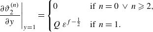 \begin{equation} \left .\frac {\partial \vartheta _{2}^{(n)}}{\partial y}\right |_{y=1} = \begin{cases} 0 & \text{if}\,\, n=0\,\vee \,n\geqslant 2, \\[6pt] Q\,\varepsilon ^{f-\frac {1}{2}} & \text{if}\,\, n=1. \end{cases} \end{equation}
C.2 Order
$\mathcal{O}(1)$
:
$\vartheta _{j}^{(0)}$
solutions


The leading-order equation (C3a
) and the boundary conditions (C6), (C7) for $n=0$
are homogeneous. This ensures that the boundary-value problem
$n=0$
are homogeneous. This ensures that the boundary-value problem
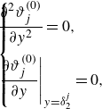 \begin{align} \left \{\!\!\!\!\!\! \begin{array}{ll}&\dfrac {\partial ^2 \vartheta _{j}^{(0)}}{\partial y^2} \def\lumina\hspace {0.7cm}= 0\,\!,\\[12pt] &\left .\dfrac {\partial \vartheta _{j}^{(0)}}{\partial y}\right |_{y=\delta _{2}^{j}} = 0\,\!,\end{array} \right . \end{align}
admits a trivial solution (i.e. that $\vartheta _{j}^{(0)}$
is independent of
$\vartheta _{j}^{(0)}$
is independent of $y$
), and, therefore,
$y$
), and, therefore, $\vartheta _{j}^{(0)} (\xi, \,\tau )$
corresponds to the average dimensionless temperature
$\vartheta _{j}^{(0)} (\xi, \,\tau )$
corresponds to the average dimensionless temperature $\langle \vartheta _{j}\rangle (\xi, \,\tau )$
defined by (3.4). This is true as long as
$\langle \vartheta _{j}\rangle (\xi, \,\tau )$
defined by (3.4). This is true as long as $p\lt 1/2$
,
$p\lt 1/2$
, $p-a\lt 1/2$
and
$p-a\lt 1/2$
and $f\gt 0$
, namely
$f\gt 0$
, namely ${\textit{Pe}}\ll 1/\sqrt {\varepsilon }$
,
${\textit{Pe}}\ll 1/\sqrt {\varepsilon }$
, $\mathcal{A}\,{\textit{Pe}}\ll 1/\sqrt {\varepsilon }$
and
$\mathcal{A}\,{\textit{Pe}}\ll 1/\sqrt {\varepsilon }$
and $q_{w}\ll 1$
– viscous dissipation also has to enter the problem as an
$q_{w}\ll 1$
– viscous dissipation also has to enter the problem as an $\mathcal{O}(\sqrt {\varepsilon })$
contribution or lower.
$\mathcal{O}(\sqrt {\varepsilon })$
contribution or lower.
C.3 Order
$\mathcal{O}(\sqrt {\varepsilon })$
:
${\vartheta }_{j}^{(1)}$
solutions


At the order $\mathcal{O} (\sqrt {\varepsilon } )$
, the derivation will be carried out without choosing a specific value for the velocity of the reference frame
$\mathcal{O} (\sqrt {\varepsilon } )$
, the derivation will be carried out without choosing a specific value for the velocity of the reference frame $V$
, which will remain arbitrary. This issue will be discussed in § 4.
$V$
, which will remain arbitrary. This issue will be discussed in § 4.
Starting from the inner phase, (C3b
) and (C6) with $n=1$
and
$n=1$
and $j=1$
give the following boundary-value problem:
$j=1$
give the following boundary-value problem:
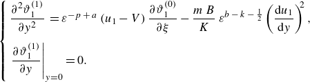 \begin{align} \left \{\begin{array}{ll} \dfrac {\partial ^2 \vartheta _{1}^{(1)}}{\partial y^2} \def\lumina\hspace {0.5cm}\,= \varepsilon ^{-p\,+\,a} \left ({u}_{1} - V\right )\dfrac {\partial \vartheta _{1}^{(0)}}{\partial \xi } - \dfrac {m\,B}{K}\,\varepsilon ^{b\,-\,k\,-\,\frac {1}{2} }\left (\dfrac {\mathrm{d}{u}_{1}}{\mathrm{d}{y}}\right )^{\!\!2}\,\!,\\[14pt] \left .\dfrac {\partial \vartheta _{1}^{(1)}}{\partial y}\right |_{y=0} = 0\,\!. \end{array}\right . \end{align}
Integrating (C9a
) with respect to $y$
gives
$y$
gives
 \begin{equation} \frac {\partial \vartheta _{1}^{(1)}}{\partial y}(y)=\frac {\varepsilon ^{a}}{\varepsilon ^{p}}\left (\int \left ({u}_{1}(y^{\ast }) - V\right )\mathrm{d}y^{\ast }\right ) \frac {\partial \vartheta _{1}^{(0)}}{\partial \xi } - \frac {m\,B}{K}\,\frac {\varepsilon ^{b\,-\,k}}{\sqrt {\varepsilon }}\int \left (\frac {\mathrm{d}u_{1}(y^{\ast })}{\mathrm{d}y^{\ast }}\right )^{\!\!2}\mathrm{d}y^{\ast } + A_{1}^{(1)}, \end{equation}
where the integration constant $A_{1}^{(1)}=0$
is determined by using the thermal symmetry condition (C9b
) along with the corresponding velocity profiles (A5).
$A_{1}^{(1)}=0$
is determined by using the thermal symmetry condition (C9b
) along with the corresponding velocity profiles (A5).
Then, we proceed by integrating (C10), obtaining
 \begin{equation} \vartheta _{1}^{(1)}(y)=\frac {\varepsilon ^{a}}{\varepsilon ^{p}}\left (\!\int \!\!\!\int\!\! \left ({u}_{1}(y^{\ast }) - V\right )\mathrm{d}^{2}y^{\ast }\!\right ) \frac {\partial \vartheta _{1}^{(0)}}{\partial \xi } - \frac {m\,B}{K}\,\frac {\varepsilon ^{b\,-\,k}}{\sqrt {\varepsilon }}\int \!\!\!\int\!\! \left (\frac {\mathrm{d}u_{1}(y^{\ast })}{\mathrm{d}y^{\ast }}\!\right )^{\!\!2}\!\mathrm{d}^{2}y^{\ast } \,+\,B_{1}^{(1)}, \end{equation}
where the integration constant $B_{1}^{(1)}$
is determined enforcing the gauge-fixing condition of the type of (3.5), i.e.
$B_{1}^{(1)}$
is determined enforcing the gauge-fixing condition of the type of (3.5), i.e. $\left \langle \vartheta _{1}^{(1)}\right \rangle =0$
(see Mikelić et al. (Reference Mikelić, Devigne and van Duijn2006)). Doing so, we get an expression for the first-order correction of the temperature of the inner phase
$\left \langle \vartheta _{1}^{(1)}\right \rangle =0$
(see Mikelić et al. (Reference Mikelić, Devigne and van Duijn2006)). Doing so, we get an expression for the first-order correction of the temperature of the inner phase
 \begin{equation} \vartheta _{1}^{(1)}\left (\xi, \,y,\,\tau ;\,\varepsilon \right )=\varepsilon ^{-p\,+\,a}\,\mathcal{M}_{1}(y)\, \frac {\partial \vartheta _{1}^{(0)}}{\partial \xi }\,-\,\frac {m\,B}{K}\,\varepsilon ^{b\,-\,k\,-\,\frac {1}{2}}\, \mathcal{M}_{1}^{\mathcal{W}}(y), \end{equation}
where the functions
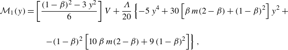 \begin{align} \mathcal{M}_{1}(y)&=\left [\frac {(1-\beta )^2-3\,y^2}{6}\right ]V+\frac {\Lambda }{20} \left \{-5\,y^4+30\left [\beta \,m(2-\beta)+\left (1-\beta \right )^2\right ]y^2\,+ \right. \nonumber \\[12pt] &\qquad \left. - (1-\beta )^2\left [10\,\beta \,m(2-\beta)+9\left (1-\beta \right )^2\right ]\right \}, \end{align}
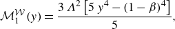 \begin{align} \mathcal{M}_{1}^{\mathcal{W}}(y)&=\frac {3\,\Lambda ^{2}\left [5\,y^4-\left (1-\beta \right )^4\right ]}{5}, \end{align}
are traditionally named B-fields after the seminal works of H. Brenner (Brenner & Stewartson Reference Brenner and Stewartson1980; Brenner & Edwards Reference Brenner and Edwards1993) on Taylor dispersion. These functions represent the mean axial displacement at long times of a fluid particle located at $y$
within the channel cross-section, under the assumption that its initial positions are all equally probable (Mauri Reference Mauri2015).
$y$
within the channel cross-section, under the assumption that its initial positions are all equally probable (Mauri Reference Mauri2015).
For the outer phase, $j=2$
, (C3b
) and (C7) for
$j=2$
, (C3b
) and (C7) for $n=1$
give
$n=1$
give
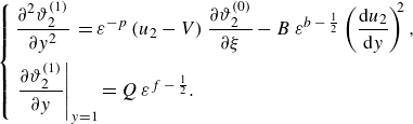 \begin{align} \left\{\begin{array}{l} \displaystyle\frac {\partial ^2 \vartheta _{2}^{(1)}}{\partial y^2} \def\lumina\hspace {0.5cm}\,= \varepsilon ^{-p} \left ({u}_{2} - V\right )\displaystyle\frac {\partial \vartheta _{2}^{(0)}}{\partial \xi } - B\,\varepsilon ^{b\,-\,\frac {1}{2} }\left (\displaystyle\frac {\mathrm{d}{u}_{2}}{\mathrm{d}{y}}\right )^{\!\!2}\,\!,\\[12pt] \left . \displaystyle\frac {\partial \vartheta _{2}^{(1)}}{\partial y}\right |_{y=1} = Q\,\varepsilon ^{f\,-\, \frac {1}{2}}\,\!. \end{array}\right. \end{align}
Following the same mathematical procedure illustrated earlier yields a solution for $\vartheta _{2}^{(1)}$
in a similar form:
$\vartheta _{2}^{(1)}$
in a similar form:
 \begin{equation} \vartheta _{2}^{(1)}\left (\xi, \,y,\,\tau ;\,\varepsilon \right )=\varepsilon ^{-p}\, \mathcal{M}_{2}(y)\, \frac {\partial \vartheta _{2}^{(0)}}{\partial \xi }\,-\,B\,\varepsilon ^{b\,-\,\frac {1}{2}}\, \mathcal{M}_{2}^{\mathcal{W}}(y)\,+\, Q\,\varepsilon ^{f\,-\,\frac {1}{2}}\,\mathcal{M}_{2}^{q}(y) \,\!, \end{equation}
where
 \begin{align} \mathcal{M}_{2}(y)&=\left [\frac {\beta ^{2}-3 \left (1-y\right )^{2}}{6}\right ]V+\frac {\Lambda \,m}{20} \left (-5\,y^{4}+30\,y^{2}-40\,y+\beta ^{4}-5\,\beta ^{3}+15\right ), \end{align}
 \begin{align} \mathcal{M}_{2}^{\mathcal{W}}(y)&= \frac {3\,\Lambda ^{2}\,m^{2}}{5}\left (-5\,y^{4}+20\,y+\beta ^{4}-5 \beta ^{3}+10 \beta ^{2}-15\right ), \end{align}
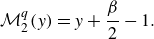 \begin{align} \mathcal{M}_{2}^{q}(y)&=y+\frac {\beta }{2}-1. \end{align}
C.4 Order
$\mathcal{O}(\varepsilon )$
:
$\vartheta _{j}^{(2)}$
solutions


At the order $\mathcal{O}(\varepsilon )$
, the procedure to find
$\mathcal{O}(\varepsilon )$
, the procedure to find $\vartheta _{j}^{(2)}$
can be simultaneously applied to both phases using the Kronecker delta defined in (3.7). First, since the previous-order solutions
$\vartheta _{j}^{(2)}$
can be simultaneously applied to both phases using the Kronecker delta defined in (3.7). First, since the previous-order solutions $\vartheta _{j}^{(1)}$
, see (C12), (C15), depend on the axial coordinate
$\vartheta _{j}^{(1)}$
, see (C12), (C15), depend on the axial coordinate $\xi$
only via the leading-order temperatures
$\xi$
only via the leading-order temperatures $\vartheta _{j}^{(0)}$
, we have
$\vartheta _{j}^{(0)}$
, we have
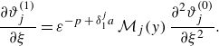 \begin{equation} \frac {\partial \vartheta ^{(1)}_{j}}{\partial \xi }=\varepsilon ^{-p\,+\,\delta _{1}^{j}a}\,\mathcal{M}_{j}(y)\,\frac {\partial ^{2} \vartheta ^{(0)}_{j}}{\partial \xi ^{2}}. \end{equation}
Then, we can replace (C17) into (C3c ) and use the boundary conditions (C6), (C7) to obtain
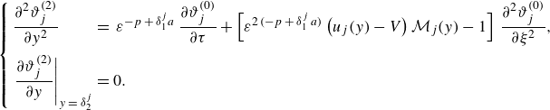 \begin{align} \left \{\begin{array}{ll} \dfrac {\partial ^2 \vartheta _{j}^{(2)}}{\partial y^2}\def\lumina\hspace {0.6cm} &=\, \varepsilon ^{-p\,+\,\delta _{1}^{j}a}\,\dfrac {\partial \vartheta _{j}^{(0)}}{\partial \tau } + \left [\varepsilon ^{2\,(-p\,+\,\delta _{1}^{j}\,a)}\left (u_{j}(y)-V\right )\mathcal{M}_{j}(y)-1\right ]\,\dfrac {\partial ^{2} \vartheta _{j}^{(0)}}{\partial \xi ^{2}}, \\[12pt] \left .\dfrac {\partial \vartheta _{j}^{(2)}}{\partial y}\right |_{y\,=\,\delta _{2}^{j}} &= 0\,\!. \end{array}\right . \end{align}
Integrating (C18a
) between $\delta _{2}^{j}$
and
$\delta _{2}^{j}$
and $y$
and making use of (C18b
) lead to
$y$
and making use of (C18b
) lead to
 \begin{equation} \frac {\partial \vartheta _{j}^{(2)}}{\partial y}(y)\,=\, \varepsilon ^{-p\,+\,\delta _{1}^{j}a}\,\varphi _{j}(y)\,\frac {\partial \vartheta _{j}^{(0)}}{\partial \tau }\, +\left [\varepsilon ^{2\,(-p\,+\,\delta _{1}^{j}\,a)}\,\psi _{j}(y)-\varphi _{j}(y)\,\right ]\,\frac {\partial ^{2} \vartheta _{j}^{(0)}}{\partial \xi ^{2}}, \end{equation}
with
 \begin{equation} \varphi _{j}(y)=\int _{\delta _{2}^{j}}^{y}\,\mathrm{d}y^{\ast }, \qquad \psi _{j}(y)=\int _{\delta _{2}^{j}}^{y}\,\mathcal{I}_{j}(y^{\ast })\,\mathrm{d}y^{\ast }, \qquad \mathcal{I}_{j}(y)=\left (u_{j}(y)-V\right )\mathcal{M}_{j}(y). \end{equation}
Integrating (C19) indefinitely gives
 \begin{equation} \vartheta _{j}^{(2)}(y)\,=\, \varepsilon ^{-p\,+\,\delta _{1}^{j}a}\,\tilde {\Phi }_{j}(y)\,\frac {\partial \vartheta _{j}^{(0)}}{\partial \tau }\, +\left [\varepsilon ^{2\,(-p\,+\,\delta _{1}^{j}\,a)}\,\tilde {\Psi }_{j}(y)-\tilde {\Phi }_{j}(y)\,\right ]\,\frac {\partial ^{2} \vartheta _{j}^{(0)}}{\partial \xi ^{2}}+B_{j}^{(2)}, \end{equation}
where
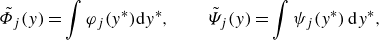 \begin{equation} \tilde {\Phi }_{j}(y)=\int \varphi _{j}(y^{\ast })\mathrm{d}y^{\ast }, \qquad \tilde {\Psi }_{j}(y)=\int \psi _{j}(y^{\ast })\,\mathrm{d}y^{\ast }, \end{equation}
and $B_{j}^{(2)}$
is an integration constant, which can be found via the gauge-fixing condition
$B_{j}^{(2)}$
is an integration constant, which can be found via the gauge-fixing condition $\langle \vartheta _{j}^{(2)}\rangle =0$
. Finally, we obtain the full expression for the second-order correction of the temperature for both phases:
$\langle \vartheta _{j}^{(2)}\rangle =0$
. Finally, we obtain the full expression for the second-order correction of the temperature for both phases:
 \begin{align} \vartheta _{j}^{(2)}\left (\xi, \,y,\,\tau ;\,\varepsilon \right )\,=\, \varepsilon ^{-p\,+\,\delta _{1}^{j}a}\,\Phi _{j}(y)\,\frac {\partial \vartheta _{j}^{(0)}}{\partial \tau }\, +\left [\varepsilon ^{2\,(-p\,+\,\delta _{1}^{j}\,a)}\,\Psi _{j}(y)-\Phi _{j}(y)\,\right ]\,\frac {\partial ^{2} \vartheta _{j}^{(0)}}{\partial \xi ^{2}}\,\!,\nonumber\\[3pt] \end{align}
with
 \begin{equation} {\Phi }_{j}(y)= \tilde {\Phi }_{j}-\big \langle \tilde {\Phi }_{j}\big \rangle, \qquad {\Psi }_{j}(y)= \tilde {\Psi }_{j}-\big \langle \tilde {\Psi }_{j}\big \rangle . \end{equation}
By inspection of (C23), we can notice that the $\mathcal{O}(\varepsilon )$
temperature profile describes the temporary thermal fluctuations occurring within the system through a time-derivative and a diffusive term. We do not report here the full analytic expression for the
$\mathcal{O}(\varepsilon )$
temperature profile describes the temporary thermal fluctuations occurring within the system through a time-derivative and a diffusive term. We do not report here the full analytic expression for the $y$
-dependent functions that define the
$y$
-dependent functions that define the $\mathcal{O}(\varepsilon )$
solution, since we will follow the approach presented by Ling et al. (Reference Ling, Tartakovsky and Battiato2016) for closing the problem (see § C.5), where we will make use only of the value that (C19), (C23) assume at the interface. To lighten notation, the inverted circumflex accent will be employed to denote the evaluation of a given function at the interface, namely
$\mathcal{O}(\varepsilon )$
solution, since we will follow the approach presented by Ling et al. (Reference Ling, Tartakovsky and Battiato2016) for closing the problem (see § C.5), where we will make use only of the value that (C19), (C23) assume at the interface. To lighten notation, the inverted circumflex accent will be employed to denote the evaluation of a given function at the interface, namely $\check {\mathcal{M}}_{j}\equiv \left .\mathcal{M}_{j}(y)\right |_{y=1-\beta }$
.
$\check {\mathcal{M}}_{j}\equiv \left .\mathcal{M}_{j}(y)\right |_{y=1-\beta }$
.
C.5 Closure of the upscaled model
To derive the upscaled model, the cross-sectional average operator (3.4) is applied to (C2) while accounting for the boundary conditions. This is a necessary and sufficient condition for the cascade of linear equations (C3) to be solvable, thereby enforcing the solvability condition.
Thus, applying the gauge condition (3.6) to the expanded energy equation for the outer phase (C2), $j=2$
, we obtain
$j=2$
, we obtain
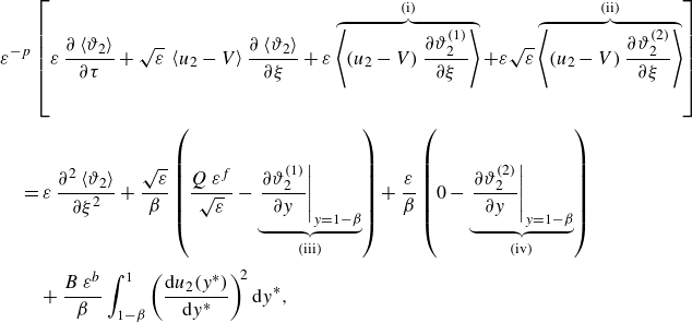 \begin{align} &\varepsilon ^{-p} \left [\varepsilon \,\frac {\partial \left \langle \vartheta _{2}\right \rangle }{\partial \tau }+ \sqrt {\varepsilon }\,\left \langle u_{2}-V\right \rangle \frac {\partial \left \langle \vartheta _{2}\right \rangle }{\partial \xi }+ \varepsilon \overbrace {\left \langle \left (u_{2}-V\right )\frac {\partial \vartheta _{2}^{(1)}}{\partial \xi }\right \rangle }^{\mathrm{(i)}}+ \varepsilon \sqrt {\varepsilon }\overbrace {\left \langle \left (u_{2}-V\right )\frac {\partial \vartheta _{2}^{(2)}}{\partial \xi }\right \rangle }^{\mathrm{(ii)}} \right ] \nonumber \\[3pt] &\quad = \varepsilon \,\frac {\partial ^{2} \left \langle \vartheta _{2}\right \rangle }{\partial \xi ^{2}}+ \frac {\sqrt {\varepsilon }}{\beta }\left (\frac {Q\,\varepsilon ^{f}}{\sqrt {\varepsilon }}-\underbrace {\left .\frac {\partial \vartheta _{2}^{(1)}}{\partial y}\right |_{y=1-\beta }}_{\mathrm{(iii)}}\right ) + \frac {{\varepsilon }}{\beta }\left (0-\underbrace {\left .\frac {\partial \vartheta _{2}^{(2)}}{\partial y}\right |_{y=1-\beta }}_{\mathrm{(iv)}}\right ) \nonumber \\[3pt] &\qquad + \frac {B\,\varepsilon ^{b}}{\beta }\int _{1-\beta }^{1} \left (\frac {\mathrm{d}u_{2}(y^{\ast })}{\mathrm{d}y^{\ast }}\right )^{\!2} \mathrm{d}y^{\ast }, \end{align}
where we used the wall boundary conditions (C7) at $\mathcal{O}(\sqrt {\varepsilon },\,\varepsilon )$
. Four terms in (C25) need to be closed: two non-local advective terms (i, ii), and two interfacial boundary terms (iii, iv). By means of (C17) and (C20), the term labelled by (i) can be expressed in terms of macro-scale quantities as
$\mathcal{O}(\sqrt {\varepsilon },\,\varepsilon )$
. Four terms in (C25) need to be closed: two non-local advective terms (i, ii), and two interfacial boundary terms (iii, iv). By means of (C17) and (C20), the term labelled by (i) can be expressed in terms of macro-scale quantities as $\varepsilon ^{-p} \left \langle \,\mathcal{I}_{2}\,\right \rangle {\partial ^{2}\left \langle \vartheta _{2}\right \rangle }/{\partial \xi ^{2}}$
, while the term (ii) is found to be zero by averaging (C3d
) with
$\varepsilon ^{-p} \left \langle \,\mathcal{I}_{2}\,\right \rangle {\partial ^{2}\left \langle \vartheta _{2}\right \rangle }/{\partial \xi ^{2}}$
, while the term (ii) is found to be zero by averaging (C3d
) with $j=2$
.
$j=2$
.
Based on the disparity in the thermal conductivities of the two phases, the continuity condition of thermal fluxes at the interface, see (C4), has different expressions depending on the order of magnitude of thermal conductivity ratio and, therefore, different closure relations are valid for terms (iii) and (iv). This leads to the identification of two different thermal models which may incorporate one or two equations (similarly to Quintard & Whitaker (Reference Quintard and Whitaker1993); Lewandowska & Auriault (Reference Lewandowska and Auriault2004); Lewandowska, Szymkiewicz & Auriault (Reference Lewandowska, Szymkiewicz and Auriault2005)): the cases where $k\gt 0$
(decoupled model) and the case where
$k\gt 0$
(decoupled model) and the case where $k=0$
(coupled model).
$k=0$
(coupled model).
C.5.1 Decoupled model
When $k\geqslant 1$
, term (iii) is obtained by replacing (C12) into (C4)
$k\geqslant 1$
, term (iii) is obtained by replacing (C12) into (C4)
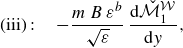 \begin{equation} \textrm {(iii)}:\quad -\frac {m\,B\,\varepsilon ^{b}}{\sqrt {\varepsilon }}\,\frac {\mathrm{d}\mathcal{\check {M}}_{1}^{\mathcal{W}}}{\mathrm{d}y}, \end{equation}
while term (iv) is zero. Thus, the upscaled energy equation describing how temperature evolves in the outer phase does not directly contain any information related to the inner flow temperature, and the resulting model is termed decoupled:
 \begin{equation} \varepsilon ^{-p}\,\frac {\partial \langle \vartheta _{2} \rangle }{\partial \tau } + \frac {\varepsilon ^{-p}}{\sqrt {\varepsilon }} \langle u_{2}-V \rangle \frac {\partial \langle \vartheta _{2} \rangle }{\partial \xi } = \left [1+\varepsilon ^{\,-2p}\,D_{2}\right ]\frac {\partial ^{2} \langle \vartheta _{2} \rangle }{\partial \xi ^{2}} + \frac {Q}{\beta }\,\varepsilon ^{f-1} +\frac {B}{\beta }\,\varepsilon ^{b-1}\,W_{2}^{\star }, \end{equation}
where the integral contributions to effective diffusivity and viscous dissipation have been denoted for brevity as follows:
 \begin{equation} D_{2}=-\left \langle \,\mathcal{I}_{2}\,\right \rangle, \qquad W_{2}^{\star }=W_{2}+m\,\,\frac {\mathrm{d}\mathcal{\check {M}}_{1}^{\mathcal{W}}}{\mathrm{d}y}, \qquad W_{2}=\int _{1-\beta }^{1} \left (\frac {\mathrm{d}u_{2}(y^{\ast })}{\mathrm{d}y^{\ast }}\right )^{\!2} \mathrm{d}y^{\ast }. \end{equation}
The full expressions of the above effective coefficients are give later on in Appendix C.6, see (C40b
) and (C46c
). After multiplying both sides of (C27) by $\varepsilon ^{p}$
, reintroducing dimensionless groups according to (3.2) and scaling back the spatial variable
$\varepsilon ^{p}$
, reintroducing dimensionless groups according to (3.2) and scaling back the spatial variable $\xi \mapsto z$
via (3.1), we obtain a one-dimensional ADHT equation for the averaged temperature of the outer phase whose full expression is given in (3.10).
$\xi \mapsto z$
via (3.1), we obtain a one-dimensional ADHT equation for the averaged temperature of the outer phase whose full expression is given in (3.10).
A special scenario is represented for the case where $k=1/2$
: the
$k=1/2$
: the $\mathcal{O}(\sqrt {\varepsilon })$
solution for the inner phase (C12) yields the following closure:
$\mathcal{O}(\sqrt {\varepsilon })$
solution for the inner phase (C12) yields the following closure:
 \begin{equation} \textrm {(iv)}:\quad K\,\varepsilon ^{-p+a}\,\frac {\mathcal{\check {M}}_{1}}{\mathrm{d}y}\,\frac {\partial \left \langle \vartheta _{1}\right \rangle }{\partial \xi }, \end{equation}
while term (iii) is the same as for the case where $k=0$
. Using (C29) leads to a single-equation model of the form of (C25) but requires an a priori knowledge of the axial gradient of the temperature of the inner phase
$k=0$
. Using (C29) leads to a single-equation model of the form of (C25) but requires an a priori knowledge of the axial gradient of the temperature of the inner phase ${\partial \left \langle \vartheta _{1}\right \rangle }/{\partial \xi }$
, reducing to the ADHT equation valid for
${\partial \left \langle \vartheta _{1}\right \rangle }/{\partial \xi }$
, reducing to the ADHT equation valid for $k\geqslant 1$
only if the inner phase has a uniform temperature. Thus, this case will not be addressed in this work.
$k\geqslant 1$
only if the inner phase has a uniform temperature. Thus, this case will not be addressed in this work.
C.5.2 Coupled model
When $k=0$
, the thermal conductivities of the two phases are comparable and the upscaled model consists of two coupled equations in the unknowns
$k=0$
, the thermal conductivities of the two phases are comparable and the upscaled model consists of two coupled equations in the unknowns $\left \langle \vartheta _{j}\right \rangle$
. Specifically, the boundary terms (iii), (iv) in (C25) are closed using (C4), obtaining
$\left \langle \vartheta _{j}\right \rangle$
. Specifically, the boundary terms (iii), (iv) in (C25) are closed using (C4), obtaining
 \begin{align} \textrm {(iii)}:\quad & K\left .\frac {\partial \vartheta _{1}^{(1)}}{\partial y}\right |_{y=1-\beta }= K\,\varepsilon ^{-p+a}\,\frac {\mathcal{\check {M}}_{1}}{\mathrm{d}y}\,\frac {\partial \left \langle \vartheta _{1}\right \rangle }{\partial \xi } -m\,B\,\varepsilon ^{b-1}\frac {\mathrm{d}\mathcal{\check {M}}_{1}^{\mathcal{W}}}{\mathrm{d}y}, \end{align}
 \begin{align} \textrm {(iv)}:\quad & K\,\left .\frac {\partial \vartheta _{1}^{(2)}}{\partial y}\right |_{y=1-\beta }= K\,\left [\varepsilon ^{-p+a}\,\check {\varphi }_{1}\,\frac {\partial \left \langle \vartheta _{1}\right \rangle }{\partial \tau } \underbrace { + \left (\varepsilon ^{2\left (-p+a\right )}\,\check {\psi }_{1}-\check {\varphi }_{1}\right )\frac {\partial ^{2} \left \langle \vartheta _{1}\right \rangle }{\partial \xi ^{2}} }_{{(\textrm {c}_{\textrm {iii}})}} \right ], \end{align}
where we used (C12) and (C19) with $j=1$
. Using (C30b
) in (C25) introduces a coupled-derivative term, i.e.
$j=1$
. Using (C30b
) in (C25) introduces a coupled-derivative term, i.e. $\propto \varepsilon ^{-p+a}\,{\partial \left \langle \vartheta _{1}\right \rangle }/{\partial \tau }$
, giving an upscaled equation including the time derivative of
$\propto \varepsilon ^{-p+a}\,{\partial \left \langle \vartheta _{1}\right \rangle }/{\partial \tau }$
, giving an upscaled equation including the time derivative of $\left \langle \vartheta _{1}\right \rangle$
and
$\left \langle \vartheta _{1}\right \rangle$
and $\left \langle \vartheta _{2}\right \rangle$
simultaneously. To avoid this issue, we can derive the
$\left \langle \vartheta _{2}\right \rangle$
simultaneously. To avoid this issue, we can derive the $\mathcal{O}(\varepsilon )$
solution of (C23) for the inner phase,
$\mathcal{O}(\varepsilon )$
solution of (C23) for the inner phase, $\vartheta _{1}^{(2)}$
, and, evaluating it at the interface, we get an expression for replacing the time derivative in (C30b
):
$\vartheta _{1}^{(2)}$
, and, evaluating it at the interface, we get an expression for replacing the time derivative in (C30b
):
 \begin{equation} \varepsilon ^{-p+a}\,\frac {\partial \left \langle \vartheta _{1}\right \rangle }{\partial \tau }=\,\frac {1}{\check {\Phi }_{1}}\left \{\left .\vartheta _{1}^{(2)}\right |_{y=1-\beta } \underbrace { -\left [\varepsilon ^{2\,(-p+a)}\,\check {\Psi }_{1}-\check {\Phi }_{1}\,\right ]\,\frac {\partial ^{2} \left \langle \vartheta _{1}\right \rangle }{\partial \xi ^{2}} }_{(\textrm {c}_{\textrm {ii}})} \right \}. \end{equation}
The last step is to enforce the continuity of temperature at the interface (C5) asymptotically, replacing the interfacial temperature in (C31) as the following power series:
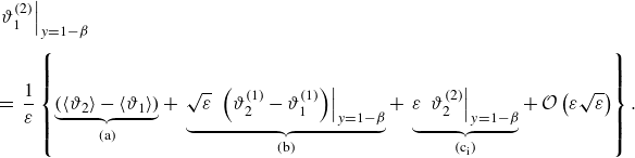 \begin{eqnarray} && \left .\vartheta _{1}^{(2)}\right |_{y=1-\beta } \nonumber\\[4pt]&& =\,\frac {1}{\varepsilon }\left \{ \underbrace {\left (\left \langle \vartheta _{2}\right \rangle -\left \langle \vartheta _{1}\right \rangle \right )}_{\text{(a)}} +\, \underbrace {\sqrt {\varepsilon }\,\left .\left (\vartheta _{2}^{(1)}-\vartheta _{1}^{(1)}\right )\right |_{y=1-\beta }}_{\text{(b)}} +\, \underbrace {\varepsilon \,\left .\vartheta _{2}^{(2)}\right |_{y=1-\beta }}_{(\textrm {c}_{\textrm {i}})} +\, \mathcal{O}\left (\varepsilon \sqrt {\varepsilon }\right ) \right \}. \nonumber\\\end{eqnarray}
This procedure shows that three different mechanisms are needed to adequately capture the thermal interplay between the phases, namely a storage-type term (a), coupled advective contributions due to axial gradients, term (b), and time-dependent/diffusive contributions, term (c). Specifically, term (b) is obtained as the difference between the $\mathcal{O}(\sqrt {\varepsilon })$
solutions, see (C12), (C15), evaluated at the interface, whereas term (c) can be detailed as follows: term
$\mathcal{O}(\sqrt {\varepsilon })$
solutions, see (C12), (C15), evaluated at the interface, whereas term (c) can be detailed as follows: term $(\textrm {c}_{\textrm {i}})$
follows from (C23) (with
$(\textrm {c}_{\textrm {i}})$
follows from (C23) (with $j=2$
), thus containing a time-derivative (
$j=2$
), thus containing a time-derivative ( $\propto \partial \left \langle \vartheta _{2}\right \rangle /\partial \tau$
) and a direct-diffusive term (
$\propto \partial \left \langle \vartheta _{2}\right \rangle /\partial \tau$
) and a direct-diffusive term ( $\propto \partial ^{2}\left \langle \vartheta _{2}\right \rangle /\partial \xi ^{2}$
), while terms
$\propto \partial ^{2}\left \langle \vartheta _{2}\right \rangle /\partial \xi ^{2}$
), while terms $(\textrm {c}_{\textrm {ii}})$
and
$(\textrm {c}_{\textrm {ii}})$
and $(\textrm {c}_{\textrm {iii}})$
results in cross-diffusion (
$(\textrm {c}_{\textrm {iii}})$
results in cross-diffusion ( $\propto \partial ^{2}\left \langle \vartheta _{1}\right \rangle /\partial \xi ^{2}$
). Note that existing transport models between coupled layers have postulated the coupling only in the form of a storage term (Reichert & Wanner Reference Reichert and Wanner1991; Kazezyılmaz-Alhan Reference Kazezyılmaz-Alhan2008) or, additionally, an advective contribution due to axial gradients (Ling et al. Reference Ling, Tartakovsky and Battiato2016, Reference Ling, Rizzo, Battiato and de Barros2021, Reference Ling, Shan and de Barros2024), but our analysis highlights that also cross-diffusive terms emerge naturally from the derivation of the model via asymptotic expansions and should be accounted for to preserve the model consistency.
$\propto \partial ^{2}\left \langle \vartheta _{1}\right \rangle /\partial \xi ^{2}$
). Note that existing transport models between coupled layers have postulated the coupling only in the form of a storage term (Reichert & Wanner Reference Reichert and Wanner1991; Kazezyılmaz-Alhan Reference Kazezyılmaz-Alhan2008) or, additionally, an advective contribution due to axial gradients (Ling et al. Reference Ling, Tartakovsky and Battiato2016, Reference Ling, Rizzo, Battiato and de Barros2021, Reference Ling, Shan and de Barros2024), but our analysis highlights that also cross-diffusive terms emerge naturally from the derivation of the model via asymptotic expansions and should be accounted for to preserve the model consistency.
The upscaled energy equation for the inner phase can be obtained following the same procedure shown in § C.5 with $j=1$
and using the symmetry condition (C6) at the channel centre line (the detailed derivation is not shown here for the sake of brevity); this gives
$j=1$
and using the symmetry condition (C6) at the channel centre line (the detailed derivation is not shown here for the sake of brevity); this gives
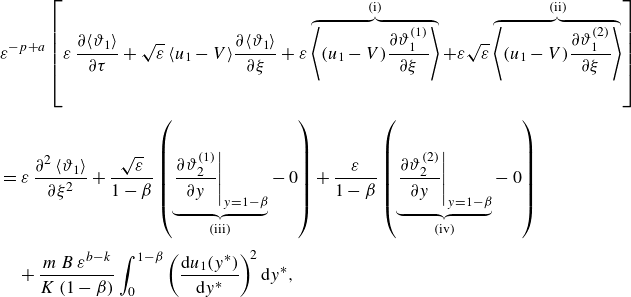 \begin{align} & \varepsilon ^{-p+a} \left [\varepsilon \,\frac {\partial \langle \vartheta _{1} \rangle }{\partial \tau }+ \sqrt {\varepsilon }\, \langle u_{1}-V \rangle \frac {\partial \langle \vartheta _{1} \rangle }{\partial \xi }+ \varepsilon \overbrace {\left \langle (u_{1}-V)\frac {\partial \vartheta _{1}^{(1)}}{\partial \xi }\right \rangle }^{\mathrm{(i)}}+ \varepsilon \sqrt {\varepsilon }\overbrace {\left \langle (u_{1}-V)\frac {\partial \vartheta _{1}^{(2)}}{\partial \xi }\right \rangle }^{\mathrm{(ii)}} \right ] \nonumber\\[4pt] & = \varepsilon \,\frac {\partial ^{2} \left \langle \vartheta _{1}\right \rangle }{\partial \xi ^{2}}+ \frac {\sqrt {\varepsilon }}{1-\beta }\left (\underbrace {\left .\frac {\partial \vartheta _{2}^{(1)}}{\partial y}\right |_{y=1-\beta }}_{\mathrm{(iii)}} -\, 0\right ) + \frac {{\varepsilon }}{1-\beta }\left (\underbrace {\left .\frac {\partial \vartheta _{2}^{(2)}}{\partial y}\right |_{y=1-\beta }}_{\mathrm{(iv)}} -\, 0\right ) \nonumber \\[4pt] & \quad + \frac {m\,B\,\varepsilon ^{b-k}}{K\left (1-\beta \right )}\int _{0}^{1-\beta } \left (\frac {\mathrm{d}u_{1}(y^{\ast })}{\mathrm{d}y^{\ast }}\right )^{\!2} \mathrm{d}y^{\ast },\end{align}
where, in analogy with (C28), we can define the following effective coefficients for diffusion and viscous dissipation – the full expressions are given in Appendix C.6, see (C40a ) and (C46c ):
 \begin{equation} D_{1}=-\left \langle \,\mathcal{I}_{1}\,\right \rangle, \qquad W_{1}=\int _{0}^{1-\beta } \left (\frac {\mathrm{d}u_{1}(y^{\ast })}{\mathrm{d}y^{\ast }}\right )^{\!2} \mathrm{d}y^{\ast }. \end{equation}
The closure of two advective terms (i), (ii) and two boundary terms (iii), i(v) in (C33) is obtained as before: regardless of the value of $k$
, by means of (C17) and (C20), we find that term (i) is equal to
$k$
, by means of (C17) and (C20), we find that term (i) is equal to $\varepsilon ^{-p+a} \left \langle \,\mathcal{I}_{1}\,\right \rangle {\partial ^{2}\left \langle \vartheta _{1}\right \rangle }/{\partial \xi ^{2}}$
, while term (ii) is zero by averaging equation (C3d
) with
$\varepsilon ^{-p+a} \left \langle \,\mathcal{I}_{1}\,\right \rangle {\partial ^{2}\left \langle \vartheta _{1}\right \rangle }/{\partial \xi ^{2}}$
, while term (ii) is zero by averaging equation (C3d
) with $j=1$
. Again, the closure of terms (iii) and (iv) is accomplished via the boundary conditions at the interface: for term (iii), it is sufficient to enforce at
$j=1$
. Again, the closure of terms (iii) and (iv) is accomplished via the boundary conditions at the interface: for term (iii), it is sufficient to enforce at $\mathcal{O}(\sqrt {\varepsilon })$
the continuity of thermal fluxes, see (C4), while for term (iv), this condition at
$\mathcal{O}(\sqrt {\varepsilon })$
the continuity of thermal fluxes, see (C4), while for term (iv), this condition at $\mathcal{O}(\varepsilon )$
has to be combined with the continuity of temperatures written in asymptotic terms, in analogy with (C32):
$\mathcal{O}(\varepsilon )$
has to be combined with the continuity of temperatures written in asymptotic terms, in analogy with (C32):
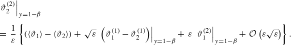 \begin{align} &\left .\vartheta _{2}^{(2)}\right |_{y=1-\beta } \nonumber\\[4pt]& =\,\frac {1}{\varepsilon }\left \{ (\left \langle \vartheta _{1}\right \rangle -\left \langle \vartheta _{2}\right \rangle ) +\, \sqrt {\varepsilon }\,\left .\left (\vartheta _{1}^{(1)}-\vartheta _{2}^{(1)}\right )\right |_{y=1-\beta } +\, \varepsilon \,\left .\vartheta _{1}^{(2)}\right |_{y=1-\beta } +\, \mathcal{O}\left (\varepsilon \sqrt {\varepsilon }\right ) \right \}. \end{align}
Finally, we obtain that heat-transfer between two flowing phases is described by the following two coupled ADHT equations:
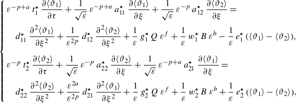 \begin{align} \left \{\begin{array}{ll} \varepsilon ^{-p+a}\,{t_1^{\star }}\,\displaystyle\frac {\partial \langle \vartheta _{1}\rangle }{\partial \tau } + \displaystyle\frac {1}{\sqrt {\varepsilon }}\,\varepsilon ^{-p+a}\,a_{11}^{\star }\,\displaystyle\frac {\partial \langle \vartheta _{1}\rangle }{\partial \xi } + \displaystyle\frac {1}{\sqrt {\varepsilon }}\,\varepsilon ^{-p}\,a_{12}^{\star }\,\displaystyle\frac {\partial \langle \vartheta _{2}\rangle }{\partial \xi } = \\[12pt] \quad d_{11}^{\star }\,\displaystyle\frac {\partial ^{2}\langle \vartheta _{1}\rangle }{\partial \xi ^{2}} + \displaystyle\frac {1}{\varepsilon ^{2p}}\,d_{12}^{\star }\,\displaystyle\frac {\partial ^{2}\langle \vartheta _{2}\rangle }{\partial \xi ^{2}} + \displaystyle\frac {1}{\varepsilon }\,{g_{1}^{\star }}\,Q\,\varepsilon ^{f} + \displaystyle\frac {1}{\varepsilon }\,{w_{1}^{\star }}\,B\,\varepsilon ^{b} - \displaystyle\frac {1}{\varepsilon }\,e_{1}^{\star }\,\big (\langle \vartheta _{1}\rangle -\langle \vartheta _{2}\rangle \big ),\def\lumina\hspace {-0.1cm}\\[16pt] \varepsilon ^{-p}\,{t_2^{\star }}\,\displaystyle\frac {\partial \langle \vartheta _{2}\rangle }{\partial \tau } + \displaystyle\frac {1}{\sqrt {\varepsilon }}\,\varepsilon ^{-p}\,a_{22}^{\star }\,\displaystyle\frac {\partial \langle \vartheta _{2}\rangle }{\partial \xi } + \displaystyle\frac {1}{\sqrt {\varepsilon }}\,\varepsilon ^{-p+a}\,a_{21}^{\star }\,\displaystyle\frac {\partial \langle \vartheta _{1}\rangle }{\partial \xi } = \\[12pt] \quad d_{22}^{\star }\,\displaystyle\frac {\partial ^{2}\langle \vartheta _{2}\rangle }{\partial \xi ^{2}} + \displaystyle\frac {\varepsilon ^{2a}}{\varepsilon ^{2p}}\,d_{21}^{\star }\,\displaystyle\frac {\partial ^{2}\langle \vartheta _{1}\rangle }{\partial \xi ^{2}} + \displaystyle\frac {1}{\varepsilon }\,{g_{2}^{\star }}\,Q\,\varepsilon ^{f} + \displaystyle\frac {1}{\varepsilon }\,{w_{2}^{\star }}\,B\,\varepsilon ^{b} + \displaystyle\frac {1}{\varepsilon }\,e_{2}^{\star }\,\big (\langle \vartheta _{1}\rangle -\langle \vartheta _{2}\rangle \big ),\def\lumina\hspace {-0.1cm} \end{array}\right . \end{align}
where the effective coefficients are defined as follows and their explicit expressions are given in Appendix C.6:
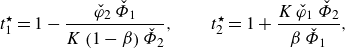 \begin{align} t_1^{\star } = 1-\frac {\check {\varphi }_{2}\,\check {\Phi }_{1}}{K\left (1-\beta \right )\check {\Phi }_{2}}, \qquad t_2^{\star } = 1+\frac {K\,\check {\varphi }_{1}\,\check {\Phi }_{2}}{\beta \,\check {\Phi }_{1}}, \end{align}
 \begin{align} a_{11}^{\star } = \left \langle u_{1}-V\right \rangle + \omega _{11}^{\star }, \quad a_{22}^{\star } = \left \langle u_{2}-V\right \rangle + \omega _{22}^{\star }, \end{align}
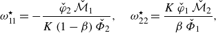 \begin{align} \omega _{11}^{\star } = - \frac {\check {\varphi }_{2}\,\check {\mathcal{M}}_{1}}{K\left (1-\beta \right )\check {\Phi }_{2}}, \quad \omega _{22}^{\star } =\frac {K\,\check {\varphi }_{1}\,\check {\mathcal{M}}_{2}}{\beta \,\check {\Phi }_{1}}, \end{align}
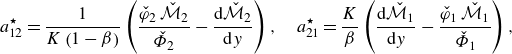 \begin{align} a_{12}^{\star } = \frac {1}{K\left (1-\beta \right )}\left (\frac {\check {\varphi }_{2}\,\check {\mathcal{M}}_{2}}{\check {\Phi }_{2}}-\frac {\mathrm{d}\check {\mathcal{M}}_{2}}{\mathrm{d}y}\right ),\quad a_{21}^{\star } = \frac {K}{\beta }\left (\frac {\mathrm{d}\check {\mathcal{M}}_{1}}{\mathrm{d}y}-\frac {\check {\varphi }_{1}\,\check {\mathcal{M}}_{1}}{\check {\Phi }_{1}}\right ), \end{align}
 \begin{align} d_{11}^{\star } = t_{1}^{\star } + \frac {\varepsilon ^{2a}}{\varepsilon ^{2p}} \left (D_{1}+\delta _{11}^{\star }\right ), \quad d_{22}^{\star } = t_{2}^{\star } + \frac {1}{\varepsilon ^{2p}} \left (D_{2}+\delta _{22}^{\star }\right ), \end{align}
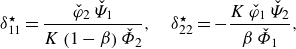 \begin{align} \delta _{11}^{\star } =\frac {\check {\varphi }_{2}\,\check {\Psi }_{1}}{K\left (1-\beta \right )\check {\Phi }_{2}}, \quad \delta _{22}^{\star } =-\frac {K\,\check {\varphi }_{1}\,\check {\Psi }_{2}}{\beta \,\check {\Phi }_{1}}, \end{align}
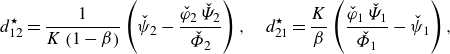 \begin{align} d_{12}^{\star } = \frac {1}{K\left (1-\beta \right )}\left (\check {\psi }_{2}-\frac {\check {\varphi }_{2}\,\check {\Psi }_{2}}{\check {\Phi }_{2}}\right ), \quad d_{21}^{\star } = \frac {K}{\beta }\left (\frac {\check {\varphi }_{1}\,\check {\Psi }_{1}}{\check {\Phi }_{1}}-\check {\psi }_{1}\right ), \end{align}
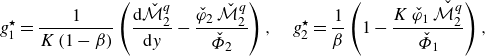 \begin{align} g_{1}^{\star } = \frac {1}{K\left (1-\beta \right )}\left (\frac {\mathrm{d}\check {\mathcal{M}}_{2}^{q}}{\mathrm{d}y}-\frac {\check {\varphi }_{2}\,\check {\mathcal{M}}_{2}^{q}}{\check {\Phi }_{2}}\right ), \quad g_{2}^{\star } = \frac {1}{\beta }\left (1-\frac {K\,\check {\varphi }_{1}\,\check {\mathcal{M}_{2}^{q}}}{\check {\Phi }_{1}}\right ), \end{align}
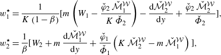 \begin{align} w_{1}^{\star } & = \frac {1}{K\left (1-\beta \right )} \bigg [ m\left (W_{1}-\frac {\check {\varphi }_{2}\,\check {\mathcal{M}}_{1}^{\mathcal{W}}}{K\,\check {\Phi }_{2}}\right ) -\frac {\mathrm{d}\check {\mathcal{M}}_{2}^{\mathcal{W}}}{\mathrm{d}y}+\frac {\check {\varphi }_{2}\,\check {\mathcal{M}}_{2}^{\mathcal{W}}}{\check {\Phi }_{2}} \bigg ],\nonumber\\\qquad w_{2}^{\star } & =\frac {1}{\beta } \bigg [W_{2}+m\,\frac {\mathrm{d}\check {\mathcal{M}}_{1}^{\mathcal{W}}}{\mathrm{d}y}+ \frac {\check {\varphi }_{1}}{\check {\Phi }_{1}}\left (K\,\check {\mathcal{M}}_{2}^{\mathcal{W}}-m\,\check {\mathcal{M}}_{1}^{\mathcal{W}}\right ) \bigg ], \end{align}
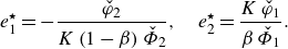 \begin{align} e_{1}^{\star } = -\frac {\check {\varphi }_{2}}{K\left (1-\beta \right )\check {\Phi }_{2}}, \quad e_{2}^{\star } = \frac {K\,\check {\varphi }_{1}}{\beta \,\check {\Phi }_{1}}. \end{align}
Reintroducing dimensionless groups and scaling back the spatial variable, we obtain the coupled model in its final form, see (3.8), (3.9).
Note that the ADHT equations of the coupled model (C37) reduce to the decoupled model in the limit of $K\to 0$
. This requires that in
$K\to 0$
. This requires that in $w_{2}^{\star }$
, we artificially remove the contribution originated by the dissipative function within the inner stream
$w_{2}^{\star }$
, we artificially remove the contribution originated by the dissipative function within the inner stream $\check {\mathcal{M}}_{1}^{\mathcal{W}}$
, which is not part of the decoupled formulation.
$\check {\mathcal{M}}_{1}^{\mathcal{W}}$
, which is not part of the decoupled formulation.
C.6 Model coefficients
The full expressions of the effective coefficients (C37) are reported below, while their physical interpretation will be given in § 4.
In particular, transient effects are taken into account via the following coefficients:
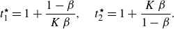 \begin{equation} t_{1}^{\star }=1+\frac {1-\beta }{K\,\beta }, \quad t_{2}^{\star }=1+\frac {K\,\beta }{1-\beta }. \end{equation}
Advective coefficients appearing in (3.8), (3.9) read
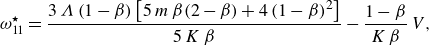 \begin{align} \omega _{11}^{\star } &= \frac {3\,\Lambda \left (1-\beta \right )\left [5\,m\,\beta (2-\beta)+4\left (1-\beta \right )^{2}\right ]}{5\,K\,\beta }-\frac {1-\beta }{K\,\beta }\,V, \end{align}
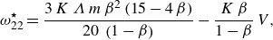 \begin{align} \omega _{22}^{\star } &= \frac {3\,K\,\Lambda \,m\,\beta ^{2}\left (15 - 4\,\beta \right )}{20\,\left (1-\beta \right )}-\frac {K\,\beta }{1-\beta }\,V, \end{align}
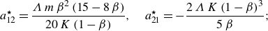 \begin{align} a_{12}^{\star } &= \frac {\Lambda \,m\,\beta ^{2}\left (15-8\,\beta \right )}{20\,K\left (1-\beta \right )}, \quad a_{21}^{\star } = -\frac {2\,\Lambda \,K\left (1-\beta \right )^{3}}{5\,\beta }; \end{align}
while effective diffusion is described by the following set of coefficients:
 \begin{align} D_{1} &= -\frac {2\,\Lambda \,\left (1 - \beta \right )^{4}}{15}\,V + \frac {2\,\Lambda ^{2}\left (1 - \beta \right )^{4}\left [7\,m\,\beta \left (2 - \beta \right ) + 6\left (1 - \beta \right )^{2}\right ]}{35}, \end{align}
 \begin{align} D_{2} &= \frac {\Lambda \,m\,\beta ^{3}\left (15 - 8\beta \right )}{60}\,V - \frac {\Lambda ^{2}\, m^{2}\,\beta ^{4}\left (8\,\beta ^{2} - 49\,\beta + 63\right )}{140}; \end{align}
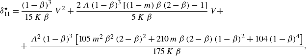 \begin{align} \delta _{11}^{\star } &= \frac {\left (1-\beta \right )^{3}}{15\,K\,\beta }\,V^{2} + \frac {2\,\Lambda \left (1-\beta \right )^{3} \left [\left (1 - m\right )\beta \,(2 - \beta ) - 1\right ]}{5\,K\,\beta }\,V +\nonumber \\[12pt] & \quad + \frac {\Lambda ^{2}\left (1 - \beta \right )^{3}\left [105\,m^{2}\,\beta ^{2}\left (2 - \beta \right )^{2} + 210\,m\,\beta \left (2 - \beta \right )\left (1 - \beta \right )^{2} + 104\left (1 - \beta \right )^{4}\right ]}{175\,K\,\beta }, \end{align}
 \begin{align} \delta _{22}^{\star } &= \frac {K\,\beta ^{3}}{15\left (1-\beta \right )}\,V^{2} + \frac {K\,\Lambda \,m\,\beta ^{4}}{8\left (1-\beta \right )}\,V -\frac {K\,\Lambda ^{2}\,m^{2}\,\beta ^{5}\left (32\,\beta ^{2} - 105\,\beta - 270\right )}{5600\,\left (1-\beta \right )}, \end{align}
 \begin{align} d_{12}^{\star } &= -\frac {\beta ^{3}}{15\,K (1 - \beta )}\,V^{2} \!+\! \frac {\Lambda \,m\,\beta ^{4} (45 \!-\! 16\,\beta )}{120\,K (1 \!-\! \beta )}\,V -\frac {\Lambda ^{2}\,m^{2}\,\beta ^{5} (288\,\beta ^{2} - 1855\,\beta + 2790 )}{5600\,K (1-\beta )}, \end{align}
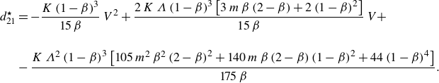 \begin{align} d_{21}^{\star } &= -\frac {K\left (1 - \beta \right )^{3}}{15\,\beta }\,V^{2} + \frac {2\,K\,\Lambda \left (1-\beta \right )^{3} \left [3\,m\,\beta \left (2 - \beta \right ) + 2\left (1 - \beta \right )^{2}\right ]}{15\, \beta }\,V + \nonumber \\[12pt] &-\frac {K\,\Lambda ^{2}\left (1 - \beta \right )^{3}\left [105\,m^{2}\,\beta ^{2}\left (2 - \beta \right )^{2} + 140\,m\,\beta \left (2 - \beta \right )\left (1 - \beta \right )^{2} + 44\left (1 - \beta \right )^{4}\right ]}{175\,\beta }. \end{align}
Among the effective coefficients, see (C37), the speed of the reference frame $V$
only impacts effective diffusion and direct-coupling advection
$V$
only impacts effective diffusion and direct-coupling advection $a_{jj}^{\star }$
. Specifically, shifting from moving to the fixed reference frame via the inverse transformation
$a_{jj}^{\star }$
. Specifically, shifting from moving to the fixed reference frame via the inverse transformation $x=z+V\,\tau$
has no net impact on diffusion, i.e.
$x=z+V\,\tau$
has no net impact on diffusion, i.e. ${\partial ^{2}\left \langle \vartheta _{j}\right \rangle }/{\partial z^{2}}\equiv {\partial ^{2}\left \langle \vartheta _{j}\right \rangle }/{\partial x^{2}}$
, but offers significant advantages in terms of the physical interpretation of the advective coefficients. In fact, each of these could be recast as the phase-averaged velocity augmented by a specific factor, namely
${\partial ^{2}\left \langle \vartheta _{j}\right \rangle }/{\partial z^{2}}\equiv {\partial ^{2}\left \langle \vartheta _{j}\right \rangle }/{\partial x^{2}}$
, but offers significant advantages in terms of the physical interpretation of the advective coefficients. In fact, each of these could be recast as the phase-averaged velocity augmented by a specific factor, namely $U_{j}^{\star }=a_{jj}^{\star }+V\,t_{jj}^{\star }=U_{j}-V+\omega _{jj}^{\star }+V\,t_{jj}^{\star }=U_{j}+\Delta U_{j}^{\star }$
, where
$U_{j}^{\star }=a_{jj}^{\star }+V\,t_{jj}^{\star }=U_{j}-V+\omega _{jj}^{\star }+V\,t_{jj}^{\star }=U_{j}+\Delta U_{j}^{\star }$
, where
 \begin{equation} \Delta U_{1}^{\star }=\frac {3\,\Lambda \left (1-\beta \right )\left [5\,m\,\beta (2-\beta)+4\left (1-\beta \right )^{2}\right ]}{5\,K\,\beta }, \quad \Delta U_{2}^{\star }=\frac {3\,K\,\Lambda \,m\,\beta ^{2}\left (15 - 4\,\beta \right )}{20\,\left (1-\beta \right )}. \end{equation}
Interestingly, the final expressions for $\Delta U_{j}^{\star }$
defined in (C43) are independent of
$\Delta U_{j}^{\star }$
defined in (C43) are independent of $V$
, implying that effective extra-advection is invariant with respect to the choice of the reference frame, i.e.
$V$
, implying that effective extra-advection is invariant with respect to the choice of the reference frame, i.e. $\left .\omega _{jj}^{\star }\right |_{V=0}\equiv \Delta U_{j}^{\star }$
.
$\left .\omega _{jj}^{\star }\right |_{V=0}\equiv \Delta U_{j}^{\star }$
.
The effective coefficients in front of the source terms in (C36) read
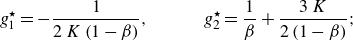 \begin{equation} g_{1}^{\star } = -\frac {1}{2\,K\left (1-\beta \right )},\qquad \quad g_{2}^{\star } = \frac {1}{\beta }+\frac {3\,K}{2\left (1-\beta \right )}; \end{equation}
whereas those concerning storage are
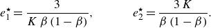 \begin{equation} e_{1}^{\star } = \frac {3}{K\,\beta \left (1-\beta \right )},\qquad \quad e_{2}^{\star } = \frac {3\,K}{\beta \left (1-\beta \right )}. \end{equation}
Finally, the analytical expressions for the effective coefficients related to viscous dissipation are
 \begin{align} w_{1}^{\star }&=\frac {3\,\Lambda ^{2}\,m\left \{4\left (1-\beta \right )^{3}\left [5\,K\beta + 3\left (1-\beta \right )\right ]-K\,m\,\beta ^{3}\left (15 - 8\,\beta \right )\right \}}{5\,K^{2}\,\beta \left (1-\beta \right )}, \end{align}
 \begin{align} w_{2}^{\star }&= \frac {3\,\Lambda ^{2}\,m\left \{m\left [3\,\beta ^{2}\,K\left (4\,\beta ^{2} \!-\! 15\,\beta + 20\right ) + 20\,\beta \left (1\!-\! \beta \right )\left (\beta ^{2}\!-\!3\beta +3\right )\right ] + 8\left (1\!-\!\beta \right )^{4}\right \}}{5\,\beta \left (1\!-\!\beta \right )}, \end{align}
 \begin{align} W_{1} &= 12\,\Lambda ^{2}\left (1 - \beta \right )^{3},\qquad W_{2} = 12\,\Lambda ^{2}\,m^{2}\,\beta \left (\beta ^{2} - 3\,\beta + 3\right ), \qquad W_{2}^{\ast } = 6\,\Lambda \,m. \end{align}
Appendix D. Model validation
To check the accuracy of the ADHT equations (3.8), (3.9), we present the validation against the steady-state solution of the problem. At the steady-state, in fact, the temperature gradients along the channel length are uniform and diffusion becomes negligible so that (in the absolute reference frame, $V=0$
)
$V=0$
)
 \begin{equation} \frac {\mathrm{d}\vartheta _{1}}{\mathrm{d}x}=\frac {\mathrm{d}\vartheta _{2}}{\mathrm{d}x}=J. \end{equation}
Consequently, the energy balances (2.13) reduce to
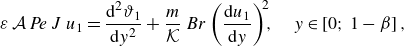 \begin{align} \varepsilon \,\mathcal{A}\,{\textit{Pe}}\,J\,u_{1} &=\frac {\mathrm{d}^{2}\vartheta _{1}}{\mathrm{d}y^{2}} +\frac {m}{\mathcal{K}}\,{Br}\left (\frac {\mathrm{d}{u}_{1}}{\mathrm{d}{y}}\right )^{\!2}\!\!,\quad y\in \left [0;\,1-\beta \right ], \end{align}
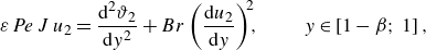 \begin{align} \varepsilon \,{\textit{Pe}}\,J\,u_{2} &=\frac {\mathrm{d}^{2}\vartheta _{2}}{\mathrm{d}y^{2}} +{Br}\left (\frac {\mathrm{d}{u}_{2}}{\mathrm{d}{y}}\right )^{\!2}\!\!,\quad \quad \, y\in \left [1-\beta ;\,1\right ], \end{align}
subjected to boundary conditions (2.16). Integrating (D2) gives
 \begin{align} \frac {\mathrm{d}\vartheta _{1}(y)}{\mathrm{d}y}&=\varepsilon \,\mathcal{A}\,{\textit{Pe}}\,J\!\int \! u_{1}(y^{\ast })\,\mathrm{d}y^{\ast } -\frac {m}{\mathcal{K}}\,{Br} \int \! \left (\frac {\mathrm{d}u_{1}(y^{\ast })}{\mathrm{d}y^{\ast }}\right )^{\!2}\mathrm{d}y^{\ast }+C_{1}, \end{align}
 \begin{align} \frac {\mathrm{d}\vartheta _{2}(y)}{\mathrm{d}y}&=\varepsilon \,{\textit{Pe}}\,J\!\int \! u_{2}(y^{\ast })\,\mathrm{d}y^{\ast } -{Br} \int \! \left (\frac {\mathrm{d}u_{2}(y^{\ast })}{\mathrm{d}y^{\ast }}\right )^{\!2}\mathrm{d}y^{\ast }+C_{2}, \end{align}
where $C_{1}$
and
$C_{1}$
and $C_{2}$
are integration constants. The value of
$C_{2}$
are integration constants. The value of $C_{1}$
is determined via the symmetry boundary condition (2.16d
), whereas the boundary condition at the wall (2.16a
) allows to express the other constant of integration as a function of the steady-state axial gradient
$C_{1}$
is determined via the symmetry boundary condition (2.16d
), whereas the boundary condition at the wall (2.16a
) allows to express the other constant of integration as a function of the steady-state axial gradient $J$
and the external heat flux
$J$
and the external heat flux $q_{w}$
, i.e. implicitly
$q_{w}$
, i.e. implicitly $C_{2}=C_{2} (q_{w},\,J,\,\ldots )$
. The expression for
$C_{2}=C_{2} (q_{w},\,J,\,\ldots )$
. The expression for $J$
can be found using the thermal flux continuity condition at the interface (2.16b
) and solving for
$J$
can be found using the thermal flux continuity condition at the interface (2.16b
) and solving for $J=J (q_{w},\ldots )$
. These calculations have been carried out using a symbolic tool and are not reported here for the sake of brevity. It can be easily checked that
$J=J (q_{w},\ldots )$
. These calculations have been carried out using a symbolic tool and are not reported here for the sake of brevity. It can be easily checked that $J$
is equivalent to the slope of the steady-state solution,
$J$
is equivalent to the slope of the steady-state solution, $M$
, of the leading-order model given in (4.21), obtaining that
$M$
, of the leading-order model given in (4.21), obtaining that $M|_{V=0}=\sqrt {\varepsilon }\,J$
.
$M|_{V=0}=\sqrt {\varepsilon }\,J$
.
Finally, aiming at validating the steady-state Nusselt number with the analytical solution of (D2), we can first integrate (D3) to obtain the steady-state temperature profile. Then, the continuity of temperatures at the interface (2.16c ) is used to eliminate one of the two additional integration constants. It is convenient to leave the constant for the outer phase temperature undetermined since it does not affect the definition of the Nusselt number (3.19): at the denominator of the local heat-transfer coefficient, only the difference between the wall and the bulk temperature appears. Doing so, the expressions of the steady-state Nusselt number obtained using the steady-state analytical solution and the upscaled model match exactly, confirming the consistency of our model.


 Open access