


1. Introduction
Exchange of mass and momentum across the interface between a porous medium and a free turbulent flow occurs in a variety of natural and industrial systems. One prominent example is the hyporheic zone, which comprises the uppermost sediment layers of a river bed, where the water in the pore space is in permanent bidirectional interaction with the overlying turbulent flow (e.g. Boano et al. Reference Boano, Harvey, Marion, Packman, Revelli, Ridolfi and Wörman2014). The hyporheic zone is characterised by a high biogeochemical activity, which makes hyporheic exchange processes highly relevant for the health of the benthic, but also the whole aquatic ecosystem (e.g. Brunke & Gonser Reference Brunke and Gonser1997; Battin et al. Reference Battin, Besemer, Bengtsson, Romani and Packmann2016). It is therefore of interdisciplinary interest to advance the understanding of the hydrodynamics near the interface between the turbulent flow and the granular, porous sediment bed.
Besides molecular diffusion, turbulent and dispersive transport can contribute to the hyporheic exchange (e.g. Voermans, Ghisalberti & Ivey Reference Voermans, Ghisalberti and Ivey2018). Turbulent transport depends on temporal fluctuations in the flow field. According to Grant et al. (Reference Grant, Gomez-Velez, Ghisalberti, Guymer, Boano, Roche and Harvey2020), those velocity fluctuations can either be induced by pressure fluctuations at the bed surface, which themselves result from turbulence in the free flow region, or can be the results of turbulent eddies entraining into the pore space. Dispersive transport, on the other hand, is associated with spatial variations in the time-averaged hyporheic flow field. Shen, Yuan & Phanikumar (Reference Shen, Yuan and Phanikumar2022) reported that even grain-scale inhomogeneities in the sediment bed surface can induce locally upwelling or downwelling fluid motion. A strong correlation between spatial variations of the time-averaged near-interface pressure field and the bed-normal time-averaged flow field is consistent with the concept of ‘pumping’, which was originally proposed by Elliott & Brooks (Reference Elliott and Brooks1997) for flow over regularly shaped macroscopic bed forms.
The analysis of the unsteady and strongly three-dimensional hyporheic flow field requires an appropriate framework. A possible approach is provided by a double-averaging technique in both time and space. First, an arbitrary flow quantity is Reynolds decomposed into a temporal mean and a temporal fluctuation. Subsequently, the temporal mean quantity is spatially averaged within a horizontal plane, which yields the double-averaged quantity and a spatial variation of the mean quantity. Initially, this method of horizontal averaging, also denoted as plane-averaging, was developed in the context of atmospheric flow problems (e.g. Wilson & Shaw Reference Wilson and Shaw1977; Raupach & Shaw Reference Raupach and Shaw1982). Later, the horizontal averaging method was adapted for the analysis of hyporheic flow problems, where drastic changes in porosity need to be taken into account (e.g. Giménez-Curto & Lera Reference Giménez-Curto and Lera1996; Nikora et al. Reference Nikora, Goring, McEwan and Griffiths2001; Mignot, Barthelemy & Hurther Reference Mignot, Barthelemy and Hurther2009). To investigate both temporal velocity fluctuations and spatial velocity variations, as well as the interactions thereof, the horizontal averaging framework can be used to conduct a triple-decomposition of the complete kinetic energy (KE) of the flow field (e.g. Raupach & Shaw Reference Raupach and Shaw1982; Yuan & Piomelli Reference Yuan and Piomelli2014; Ghodke & Apte Reference Ghodke and Apte2016). Within the double-averaging framework, the mean kinetic energy (MKE) represents the kinetic energy in the temporally and spatially double-averaged flow field. The kinetic energy in the spatial velocity variations is referred to as wake kinetic energy, or short WKE (e.g. Finnigan Reference Finnigan2000; Yuan & Piomelli Reference Yuan and Piomelli2014; Ghodke & Apte Reference Ghodke and Apte2016). The remaining third part is the spatially averaged turbulent kinetic energy (TKE), which represents the temporal fluctuations in the velocity field.
Ghodke & Apte (Reference Ghodke and Apte2018) illustrate the energy transfer pathways between the different components of the total kinetic energy. The mechanisms behind the energy transfer pathways are identified via terms which appear with opposite signs in the budget equations of MKE, WKE and TKE (Yuan & Piomelli Reference Yuan and Piomelli2014). Accordingly, two different mechanisms exist, which can generate spatial variations in the mean flow field. A transfer of MKE into WKE happens when dispersive shear stresses act against the vertical gradient of the double-averaged flow field. Also the work of the double-averaged flow field against the pressure drag generates WKE at the expense of MKE. As stated by Finnigan (Reference Finnigan2000), TKE can also be produced via two different pathways. The shear production mechanism transfers MKE into TKE when Reynolds shear stresses act against the vertical gradient of the double-averaged flow field. Besides that, form-induced production can convert WKE into TKE when the local Reynolds stresses act against local gradients introduced by velocity variations. Whereas shear production can introduce TKE on large scales, form-induced production generates TKE on the usually smaller scale of the flow obstacles, which thus ‘bypasses’ (Finnigan Reference Finnigan2000) or ‘short-circuits’ (Raupach, Antonia & Rajagopalan Reference Raupach, Antonia and Rajagopalan1991) the energy cascade.
Mignot et al. (Reference Mignot, Barthelemy and Hurther2009) conducted experimental measurements in turbulent flow over gravel beds. They report that TKE production exceeds the dissipation in the form-induced layer, which comprises the region near the crests of the roughness elements. In this context, shear production plays a dominant role, whereas form-induced production was found to be negligible. Below the roughness crests, turbulent transport relocates TKE into deeper regions of the sediment bed. In contrast, an upward TKE transport was observed above the crests, which agrees with findings for rough impermeable walls (e.g. Raupach et al. Reference Raupach, Antonia and Rajagopalan1991; Antonia & Krogstad Reference Antonia and Krogstad2001; Schultz & Flack Reference Schultz and Flack2005). At approximately twice the height of the roughness crests, Mignot et al. (Reference Mignot, Barthelemy and Hurther2009) document the presence of an equilibrium layer, as described by Townsend (Reference Townsend1961). TKE budgets in flow over porous media were also reported by several numerical studies (e.g. Breugem, Boersma & Uittenbogaard Reference Breugem, Boersma and Uittenbogaard2006; Han, He & Fang Reference Han, He and Fang2017; Fang et al. Reference Fang, Han, He and Dey2018; Wang et al. Reference Wang, Yang, Evrim, Terzis, Helmig and Chu2021). By means of pore-resolved direct numerical simulation (DNS), Shen, Yuan & Phanikumar (Reference Shen, Yuan and Phanikumar2020) investigated turbulent open-channel channel flow over sediment beds with both regular and random sphere arrangement in the interface region. In contrast to Mignot et al. (Reference Mignot, Barthelemy and Hurther2009), they observe a non-negligible impact of form-induced production, which however strongly depends on the interface structure and can even change its sign. Further, Shen et al. (Reference Shen, Yuan and Phanikumar2020) report that the randomly structured sediment–water interface enhances the form-induced vertical TKE transport, which counteracts the other transport processes. Also Fang et al. (Reference Fang, Han, He and Dey2018) document a significant form-induced production, which can even exceed 10 % of the shear production.
In contrast to the temporal velocity fluctuations, Ghodke & Apte (Reference Ghodke and Apte2018) remark that only few other studies (e.g. Yuan & Piomelli Reference Yuan and Piomelli2014; Ghodke & Apte Reference Ghodke and Apte2016) systematically investigate the production, transport and destruction of spatial variations in the horizontally averaged velocity field. Using the equations derived by Raupach & Shaw (Reference Raupach and Shaw1982) under consideration of the varying porosity, Yuan & Piomelli (Reference Yuan and Piomelli2014) evaluate the budget of WKE for the flow over transitionally and fully rough impermeable walls. The work of the horizontally double-averaged flow against the pressure drag is found to contribute significantly to the production of variation in the streamwise velocity field. Yuan & Piomelli (Reference Yuan and Piomelli2014) documented that, with increasing roughness, larger shares of the WKE are transferred into TKE instead of being dissipated, which they explain with a clearer separation between roughness length scales and the viscous length scale. The energy transfer from WKE to the wall-normal and spanwise Reynolds normal stresses was connected to a higher isotropy of the Reynolds stress tensor. In the context of a time–volume double-averaging framework, Pinson et al. (Reference Pinson, Grégoire and Simonin2006) describe a kinetic energy transfer between macro-scale and sub-filter mean kinetic energy, which corresponds to a transfer from MKE to WKE. This kinetic energy transfer results from the work of the time- and volume-averaged velocity field against the time-averaged drag. Kuwata & Suga (Reference Kuwata and Suga2015) and Kuwata & Suga (Reference Kuwata and Suga2016) represent the same mechanism by a drag force term, which was found to contribute largely to the spatial variance in the flow field. It appears worthwhile to remark that the drag also includes a viscous component, which is not considered by Raupach & Shaw (Reference Raupach and Shaw1982), Yuan & Piomelli (Reference Yuan and Piomelli2014) or Ghodke & Apte (Reference Ghodke and Apte2018).
The permeability Reynolds number $Re_K=u_\tau \sqrt {K}/\nu$
and the roughness Reynolds number
$Re_K=u_\tau \sqrt {K}/\nu$
and the roughness Reynolds number $Re_{k_s}=u_\tau k_s/\nu = k_s^+$
are commonly used parameters, as the permeability
$Re_{k_s}=u_\tau k_s/\nu = k_s^+$
are commonly used parameters, as the permeability $K$
and the equivalent sand-grain roughness height
$K$
and the equivalent sand-grain roughness height $k_s$
characterise the sediment bed. The parameters
$k_s$
characterise the sediment bed. The parameters $Re_K$
and
$Re_K$
and $k_s^+$
are connected via the sediment bed structure, such that the effects of roughness and permeability are tightly coupled for granular porous media with a narrow grain size distribution (e.g. Voermans, Ghisalberti & Ivey Reference Voermans, Ghisalberti and Ivey2017; Shen et al. Reference Shen, Yuan and Phanikumar2020; Karra et al. Reference Karra, Apte, He and Scheibe2023). The roughness Reynolds number
$k_s^+$
are connected via the sediment bed structure, such that the effects of roughness and permeability are tightly coupled for granular porous media with a narrow grain size distribution (e.g. Voermans, Ghisalberti & Ivey Reference Voermans, Ghisalberti and Ivey2017; Shen et al. Reference Shen, Yuan and Phanikumar2020; Karra et al. Reference Karra, Apte, He and Scheibe2023). The roughness Reynolds number $k_s^+$
allows a distinction between the dynamically smooth regime (
$k_s^+$
allows a distinction between the dynamically smooth regime ( $k_s^+ \lt 5$
), the transitionally rough regime and the fully rough regime (
$k_s^+ \lt 5$
), the transitionally rough regime and the fully rough regime ( $k_s^+ \gt 70$
) (Raupach et al. Reference Raupach, Antonia and Rajagopalan1991; Jiménez Reference Jiménez2004; Kadivar, Tormey & McGranaghan Reference Kadivar, Tormey and McGranaghan2021). In the smooth regime, mainly viscous stresses transfer momentum from the flow to the solid surface, whereas pressure drag on the solid surfaces gains importance with increasing
$k_s^+ \gt 70$
) (Raupach et al. Reference Raupach, Antonia and Rajagopalan1991; Jiménez Reference Jiménez2004; Kadivar, Tormey & McGranaghan Reference Kadivar, Tormey and McGranaghan2021). In the smooth regime, mainly viscous stresses transfer momentum from the flow to the solid surface, whereas pressure drag on the solid surfaces gains importance with increasing $k_s^+$
. The permeability Reynolds number
$k_s^+$
. The permeability Reynolds number $Re_K$
describes the permeability regime, as
$Re_K$
describes the permeability regime, as $\sqrt {K}$
can be interpreted as an effective pore diameter (Breugem et al. Reference Breugem, Boersma and Uittenbogaard2006; Manes, Poggi & Ridolfi Reference Manes, Poggi and Ridolfi2011; Voermans et al. Reference Voermans, Ghisalberti and Ivey2017; Karra et al. Reference Karra, Apte, He and Scheibe2023). According to the hydrodynamic framework of Voermans et al. (Reference Voermans, Ghisalberti and Ivey2017), large values of
$\sqrt {K}$
can be interpreted as an effective pore diameter (Breugem et al. Reference Breugem, Boersma and Uittenbogaard2006; Manes, Poggi & Ridolfi Reference Manes, Poggi and Ridolfi2011; Voermans et al. Reference Voermans, Ghisalberti and Ivey2017; Karra et al. Reference Karra, Apte, He and Scheibe2023). According to the hydrodynamic framework of Voermans et al. (Reference Voermans, Ghisalberti and Ivey2017), large values of $Re_K \gg 1$
indicate highly permeable boundaries, whereas low values (
$Re_K \gg 1$
indicate highly permeable boundaries, whereas low values ( $Re_K \ll 1$
) are associated with effectively impermeably boundaries. A transition between both extremes takes place in the range of
$Re_K \ll 1$
) are associated with effectively impermeably boundaries. A transition between both extremes takes place in the range of $Re_K \approx 1 {-} 2$
. High permeability, paired with roughness, relaxes the wall-blocking effect and reduces the near-interface shear intensity, which affects the structure of turbulence and the composition of the turbulent kinetic energy (e.g. Breugem et al. Reference Breugem, Boersma and Uittenbogaard2006; Rosti, Cortelezzi & Quadrio Reference Rosti, Cortelezzi and Quadrio2015; Suga, Nakagawa & Kaneda Reference Suga, Nakagawa and Kaneda2017).
$Re_K \approx 1 {-} 2$
. High permeability, paired with roughness, relaxes the wall-blocking effect and reduces the near-interface shear intensity, which affects the structure of turbulence and the composition of the turbulent kinetic energy (e.g. Breugem et al. Reference Breugem, Boersma and Uittenbogaard2006; Rosti, Cortelezzi & Quadrio Reference Rosti, Cortelezzi and Quadrio2015; Suga, Nakagawa & Kaneda Reference Suga, Nakagawa and Kaneda2017).
This overview indicates that the treatment of viscous effects may have received less attention within the horizontal averaging framework, which is likely due to the origins of the framework in atmospheric sciences. However, the same may not be justified for granular porous media in aquatic environments, where the flow is characterised by comparatively low permeability Reynolds numbers. Whilst several studies have evaluated the TKE budget near the sediment–water interface, the WKE budget has hardly been discussed for turbulent flow over porous granular beds. Due to the critical role of spatial velocity variations for hyporheic exchange, we feel that an evaluation of this budget could advance our current understanding. To our knowledge, also the scaling of different WKE and TKE budget terms over a wider parameter space covering both transitionally and fully rough regimes has not yet been documented.
Building on v.Wenczowski & Manhart (Reference v. Wenczowski and Manhart2024), the present study aims to answer the following questions: (i) which role(s) can viscous effects play for the spatial variations in the velocity field?; (ii) how do the different production mechanisms of TKE and WKE scale with $Re_K$
and
$Re_K$
and $Re_\tau$
, and at what height do they reach their peak values?; (iii) which transport mechanisms are most efficient in relocating TKE and WKE in the near-interface region? To address these question, we revisit the budget equations for MKE, WKE and TKE in § 2. The applied methods as well as the sampled parameter space with systematically varying
$Re_\tau$
, and at what height do they reach their peak values?; (iii) which transport mechanisms are most efficient in relocating TKE and WKE in the near-interface region? To address these question, we revisit the budget equations for MKE, WKE and TKE in § 2. The applied methods as well as the sampled parameter space with systematically varying $Re_\tau$
and
$Re_\tau$
and $Re_K$
are introduced in § 3. In § 4, we evaluate the TKE and WKE budgets based on datasets obtained from pore-resolved DNS, while we also shed a light on the scaling behaviour of different terms. The main results are then discussed in § 5, before § 6 concludes the study.
$Re_K$
are introduced in § 3. In § 4, we evaluate the TKE and WKE budgets based on datasets obtained from pore-resolved DNS, while we also shed a light on the scaling behaviour of different terms. The main results are then discussed in § 5, before § 6 concludes the study.
2. Theory
The governing equations are introduced in § 2.1, and important properties of the horizontal averaging framework are outlined in § 2.2. Based on the decomposition of the kinetic energy in § 2.3, we discuss the budgets of TKE, WKE and MKE in §§ 2.4, 2.5 and 2.6, respectively. Transfer mechanisms between the kinetic energy components are summarised in § 2.7.
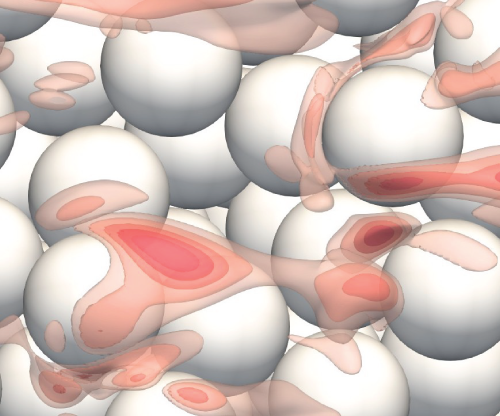
2.1. Governing equations
The incompressible Navier–Stokes equations for a Newtonian fluid with a density $\rho$
and a kinematic viscosity
$\rho$
and a kinematic viscosity $\nu$
provide the basis for the budget formulations. The Einstein summation convention allows to express the conservation of mass and momentum as follows:
$\nu$
provide the basis for the budget formulations. The Einstein summation convention allows to express the conservation of mass and momentum as follows:
 \begin{align}&\qquad\qquad\qquad\quad \frac {\partial u_i}{\partial x_i} = 0, \end{align}
 \begin{align}& \frac {\partial u_i}{\partial t} + u_j \, \frac {\partial u_i}{\partial x_j} = - \frac {1}{\rho } \frac {\partial p}{\partial x_i} + \nu \frac { \partial ^2 u_i }{ \partial x_j \partial x_j } + g_i. \end{align}
The coordinates are defined such that $x_1 \equiv x$
,
$x_1 \equiv x$
, $x_2 \equiv y$
and
$x_2 \equiv y$
and $x_3 \equiv z$
represent the streamwise, spanwise and bed-normal coordinate, respectively. The corresponding flow velocities are
$x_3 \equiv z$
represent the streamwise, spanwise and bed-normal coordinate, respectively. The corresponding flow velocities are $u_1 \equiv u$
,
$u_1 \equiv u$
, $u_2 \equiv v$
and
$u_2 \equiv v$
and $u_3 \equiv w$
. The variable
$u_3 \equiv w$
. The variable $p$
represents the pressure and
$p$
represents the pressure and $g_i$
is a volume force acting on the fluid. In (2.2), we express the viscous term as
$g_i$
is a volume force acting on the fluid. In (2.2), we express the viscous term as $\nu \, \partial ^2 u_i / \partial x_j \partial x_j$
, which is possible due to the solenoidality constraint imposed by (2.1). In the derivation of the budgets, this formulation will lead us to a pseudo-dissipation formulation (e.g. Pope Reference Pope2000). We accept the pseudo-dissipation formulation, as it abbreviates the notation and facilitates the comparison to other studies (e.g. Finnigan Reference Finnigan2000; Yuan & Piomelli Reference Yuan and Piomelli2014; Ghodke & Apte Reference Ghodke and Apte2018; Hantsis & Piomelli Reference Hantsis and Piomelli2020; Shen et al. Reference Shen, Yuan and Phanikumar2020), which similarly use this formulation. In Appendix A, we show that only minor differences between full-dissipation and pseudo-dissipation are to be expected for the budgets that are evaluated in this study.
$\nu \, \partial ^2 u_i / \partial x_j \partial x_j$
, which is possible due to the solenoidality constraint imposed by (2.1). In the derivation of the budgets, this formulation will lead us to a pseudo-dissipation formulation (e.g. Pope Reference Pope2000). We accept the pseudo-dissipation formulation, as it abbreviates the notation and facilitates the comparison to other studies (e.g. Finnigan Reference Finnigan2000; Yuan & Piomelli Reference Yuan and Piomelli2014; Ghodke & Apte Reference Ghodke and Apte2018; Hantsis & Piomelli Reference Hantsis and Piomelli2020; Shen et al. Reference Shen, Yuan and Phanikumar2020), which similarly use this formulation. In Appendix A, we show that only minor differences between full-dissipation and pseudo-dissipation are to be expected for the budgets that are evaluated in this study.
2.2. Analysis framework
To analyse the flow field, we use horizontal averaging within $x$
-
$x$
- $y$
-planes, which are parallel to the mean sediment bed surface. In a first step, the Reynolds decomposition splits an arbitrary quantity
$y$
-planes, which are parallel to the mean sediment bed surface. In a first step, the Reynolds decomposition splits an arbitrary quantity $\phi$
into an ensemble average
$\phi$
into an ensemble average $\overline {\phi }$
and a temporal fluctuation
$\overline {\phi }$
and a temporal fluctuation $\phi '$
:
$\phi '$
:
 \begin{equation} \phi _{( \boldsymbol{x},t)} = \overline {\phi }_{(\boldsymbol{x})} + \phi ^\prime _{(\boldsymbol{x},t)} \:, \hspace {1cm} \text{where} \hspace {1cm} \overline {\phi }_{(\boldsymbol{x})} = \frac {1}{T} \int _{0}^{T} \phi _{(\boldsymbol{x},t)} \: {\rm d}t. \end{equation}
In a second step, the time-averaged quantity $\overline {\phi }$
from (2.3) undergoes a decomposition with respect to space. The intrinsic average within a horizontal plane is denoted as
$\overline {\phi }$
from (2.3) undergoes a decomposition with respect to space. The intrinsic average within a horizontal plane is denoted as $\left \langle \overline {\phi } \right \rangle$
, whereas deviations from the in-plane average are marked by a tilde:
$\left \langle \overline {\phi } \right \rangle$
, whereas deviations from the in-plane average are marked by a tilde:
 \begin{equation} \overline {\phi }_{(\boldsymbol{x})} = \langle \overline {\phi } \rangle _{(z)} + \widetilde {\overline {\phi }}_{(\boldsymbol{x})} \:, \hspace {1cm} \text{where} \hspace {1cm} \langle \overline {\phi } \rangle _{(z)} = \frac {1}{A_{f}} \iint _{A_f} \overline {\phi }_{(\boldsymbol{x})} \: {\rm d}x \: {\rm d}y. \end{equation}
According to its definition in (2.4), the intrinsic average $\left \langle \overline \phi \right \rangle$
represents an average over the fluid-filled area
$\left \langle \overline \phi \right \rangle$
represents an average over the fluid-filled area $A_f$
. The superficial average
$A_f$
. The superficial average $\left \langle \overline \phi \right \rangle ^s$
, however, refers to an average over the complete base area
$\left \langle \overline \phi \right \rangle ^s$
, however, refers to an average over the complete base area $A_0$
of the averaging plane. Therefore, the in-plane porosity
$A_0$
of the averaging plane. Therefore, the in-plane porosity $\theta {(z)}$
allows a transformation between intrinsic and superficial spatial averages:
$\theta {(z)}$
allows a transformation between intrinsic and superficial spatial averages:
 \begin{equation} \langle \overline { \phi } \rangle ^s{(z)} = \theta {(z)} \: \langle \overline { \phi } \rangle {(z)} \hspace {1cm} \text{with} \hspace {1cm} \theta {(z)} = {A_{f}(z)} \, / \, {A_0}. \end{equation}
It is worthwhile to note that, in contrast to $\overline {\phi }$
and
$\overline {\phi }$
and $\phi '$
, the individual quantities
$\phi '$
, the individual quantities $\langle \overline {\phi } \rangle$
and
$\langle \overline {\phi } \rangle$
and $\widetilde {\overline {\phi }}$
do not satisfy the physical boundary conditions. In particular, the infringement of no-slip conditions on solid surfaces will give rise to terms that may appear artificial at first glance, but still allow a physical interpretation. Another consequence is that spatial derivatives and horizontal averaging operations do not commute below the crests of the sediment grains, where the area
$\widetilde {\overline {\phi }}$
do not satisfy the physical boundary conditions. In particular, the infringement of no-slip conditions on solid surfaces will give rise to terms that may appear artificial at first glance, but still allow a physical interpretation. Another consequence is that spatial derivatives and horizontal averaging operations do not commute below the crests of the sediment grains, where the area $A_f$
changes over
$A_f$
changes over $z$
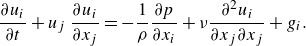
. Consistent with Giménez-Curto & Lera (Reference Giménez-Curto and Lera1996), the horizontally averaged spatial gradient of
$z$
. Consistent with Giménez-Curto & Lera (Reference Giménez-Curto and Lera1996), the horizontally averaged spatial gradient of $\overline { \phi }$
can be formulated as follows:
$\overline { \phi }$
can be formulated as follows:
 \begin{align} \displaystyle \left \langle \nabla \overline { \phi } \right \rangle = \left ( \begin{matrix} \displaystyle \left \langle \frac {\partial \overline { \phi }}{\partial x} \right \rangle \\[17pt] \displaystyle \left \langle \frac {\partial \overline { \phi }}{\partial y} \right \rangle \\[17pt] \displaystyle \left \langle \frac {\partial \overline { \phi }}{\partial z} \right \rangle \end{matrix} \right ) = \left ( \begin{matrix} \displaystyle \frac {1}{A_f} \oint _s \: \overline { \phi } \: \frac {n_x}{\sqrt {n_x^2 + n_y^2}} \: {\rm d}s \\[22pt] \displaystyle \frac {1}{A_f} \oint _s \: \overline { \phi } \: \frac {n_y}{\sqrt {n_x^2 + n_y^2}} \: {\rm d}s \\[22pt] \displaystyle \frac {1}{\theta } \frac {\partial \theta \left \langle \overline { \phi } \right \rangle }{\partial z} + \frac {1}{A_f} \oint _s \:\overline { \phi } \: \frac {n_z}{\sqrt {n_x^2 + n_y^2}} \: {\rm d}s \end{matrix} \right ) \triangleq \left ( \begin{matrix} \displaystyle BT_1( \overline { \phi } ) \\[7pt] \displaystyle BT_2( \overline { \phi } ) \\[7pt] \displaystyle \frac {1}{\theta } \frac {\partial \theta \left \langle \overline { \phi } \right \rangle }{\partial z} +BT_3( \overline { \phi } ) \end{matrix} \right ). \end{align}
The curve $s$
in (2.6) describes the intersection of the averaging plane with the fluid–solid interface, e.g. the surface of sediment grains. The unit normal vector
$s$
in (2.6) describes the intersection of the averaging plane with the fluid–solid interface, e.g. the surface of sediment grains. The unit normal vector $\boldsymbol{n} = (n_x, n_y, n_z)^T$
at the solid–fluid interface points out of the fluid-filled volume. To shorten the notation, we refer to the curve integrals as the boundary term, abbreviated as
$\boldsymbol{n} = (n_x, n_y, n_z)^T$
at the solid–fluid interface points out of the fluid-filled volume. To shorten the notation, we refer to the curve integrals as the boundary term, abbreviated as $BT_i(\overline { \phi })$
.
$BT_i(\overline { \phi })$
.
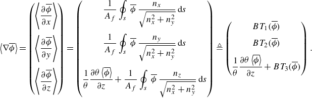
The double-averaged momentum equation is obtained by applying the above rules to (2.2). In preview of the application, we imply that $\left \langle \overline {w} \right \rangle = 0$
, which means that no net flux in the bed-normal direction exists, while no-slip boundary conditions apply on the surfaces of the sediment grains, such that
$\left \langle \overline {w} \right \rangle = 0$
, which means that no net flux in the bed-normal direction exists, while no-slip boundary conditions apply on the surfaces of the sediment grains, such that
 \begin{align} \frac {\partial \langle \overline {u} \rangle }{ \partial t} \: = \: & \frac {1}{\theta } \frac {\partial }{\partial z} \, \left ( \, \underbrace { \theta \left \langle \nu \frac {\partial \, \overline {u} }{\partial z} \right \rangle }_{visc.} \, - \, \underbrace {\theta \big\langle \overline {u^\prime w^\prime } \big\rangle }_{turb.} \, - \, \underbrace {\theta \big \langle \widetilde {\overline {u}} \, \widetilde {\overline {w}} \big\rangle }_{disp.} \, \right ) \nonumber\\ & + \: \underbrace { \frac {1}{\rho } \, BT_1( -\overline {p} ) }_{ f_{p,i} } \: + \: \underbrace { BT_j \left ( \nu \frac { \partial \overline {u} }{ \partial x_j } \right ) }_{ f_{\nu ,i} } \: + \: \langle \overline {g}_x \rangle {\: = \: 0}. \end{align}
The time derivative of the double-averaged velocity on the left-hand side is obtained from double-averaging of the time derivative of $u$
as the operators commute (Pope Reference Pope2000, § 3.6). In statistically stationary flows, the time derivatives of double-averaged quantities are zero. Equation (2.7) shows that viscous, turbulent and dispersive stresses can transfer momentum within the fluid volume. Due to their origin, dispersive stresses are also synonymously called form-induced stresses (Giménez-Curto & Lera Reference Giménez-Curto and Lera1996; Nikora et al. Reference Nikora, Goring, McEwan and Griffiths2001). Pressure drag
$u$
as the operators commute (Pope Reference Pope2000, § 3.6). In statistically stationary flows, the time derivatives of double-averaged quantities are zero. Equation (2.7) shows that viscous, turbulent and dispersive stresses can transfer momentum within the fluid volume. Due to their origin, dispersive stresses are also synonymously called form-induced stresses (Giménez-Curto & Lera Reference Giménez-Curto and Lera1996; Nikora et al. Reference Nikora, Goring, McEwan and Griffiths2001). Pressure drag $f_p$
and viscous drag
$f_p$
and viscous drag $f_\nu$
result from pressure or viscous forces, respectively, acting on solid surfaces, e.g. of the sediment grains. Thus, they represent the momentum exchange with the fluid–solid interface. A volume force in the streamwise direction is denoted as
$f_\nu$
result from pressure or viscous forces, respectively, acting on solid surfaces, e.g. of the sediment grains. Thus, they represent the momentum exchange with the fluid–solid interface. A volume force in the streamwise direction is denoted as $g_x$
. While the interpretation of pressure drag and viscous drag as boundary terms is decisive for the further derivations, the equalities in (2.6) allow us to evaluate
$g_x$
. While the interpretation of pressure drag and viscous drag as boundary terms is decisive for the further derivations, the equalities in (2.6) allow us to evaluate $f_p$
and
$f_p$
and $f_\nu$
from plane averages within an
$f_\nu$
from plane averages within an $x$
-
$x$
- $y$
-periodic domain. In Appendix B, we demonstrate that an evaluation as plane-averages is advantageous for an immersed boundary representation, while good agreement with values obtained from an actual surface integration is observed.
$y$
-periodic domain. In Appendix B, we demonstrate that an evaluation as plane-averages is advantageous for an immersed boundary representation, while good agreement with values obtained from an actual surface integration is observed.
2.3. Decomposition of the kinetic energy
The horizontal averaging framework allows a decomposition of the double-averaged total kinetic energy into three components:
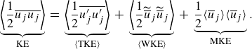 \begin{equation} \underbrace { \left \langle \frac {1}{2} \overline {u_j u_j} \right \rangle }_{\text{KE}} \: = \: \underbrace { \left \langle \frac {1}{2} \overline {u_j' u_j'} \right \rangle }_{\langle \text{TKE} \rangle } \: + \: \underbrace { \left \langle \frac {1}{2} \widetilde {\overline {u}}_j \widetilde {\overline {u}}_j \right \rangle }_{ \langle \text{WKE} \rangle } \: + \: \underbrace { \frac {1}{2} \langle \overline {u}_j \rangle \langle \overline {u}_j \rangle }_{\text{MKE}} .\end{equation}
To be consistent with the nomenclature of Finnigan (Reference Finnigan2000), Yuan & Piomelli (Reference Yuan and Piomelli2014) and Ghodke & Apte (Reference Ghodke and Apte2016), we will use the terms turbulent kinetic energy (TKE), wake kinetic energy (WKE) and mean kinetic energy (MKE) to distinguish the three terms on the right-hand side of (2.8). Together, WKE and MKE constitute the energy in the time-averaged mean flow field. The total WKE and total TKE result from the sum of all dispersive or Reynolds normal stresses, respectively. In the following, budget expressions for the total energies as well as for individual components will be presented. Like in (2.7), the time derivative of the double-averaged kinetic energies is zero in a statistically stationary flow. By checking the closure of the budget, we can assess if sufficient statistics have been sampled.
2.4. Budget equation for the TKE components
Without a summation over the Greek index $\alpha =1,2,3$
, (2.9) formulates a budget for the horizontally averaged individual TKE components, which are interconnected via an inter-component redistribution term. When summed over
$\alpha =1,2,3$
, (2.9) formulates a budget for the horizontally averaged individual TKE components, which are interconnected via an inter-component redistribution term. When summed over $\alpha$
, the budget for the horizontally averaged TKE is obtained via
$\alpha$
, the budget for the horizontally averaged TKE is obtained via
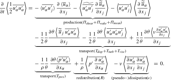 \begin{align} \frac {\partial }{\partial t} \left \langle \frac {1}{2} \overline {u^{\prime}_\alpha u^{\prime}_\alpha } \right \rangle \: = \:&\underbrace {- \: \Big \langle \overline {u^{\prime}_\alpha u^{\prime}_j} \Big \rangle \, \frac { \partial \, \langle \overline {u}_\alpha \rangle }{ \partial x_j } \: - \:\left \langle{\widetilde { \overline {u^{\prime}_\alpha u^{\prime}_j} }} \, \frac { \partial \, {\widetilde { \overline {u} }}_\alpha }{ \partial x_j } \right \rangle \: - \:\left \langle \overline {u^{\prime}_\alpha u^{\prime}_j} \right \rangle \,\left \langle\frac { \partial \, {\widetilde { \overline {u} }}_\alpha }{ \partial x_j }\right \rangle}_{ {\textrm {production} ( \Pi _{\textit {shear}} + \Pi _{\textit {wake}} + \Pi _{\textit {mean}} ) } }\nonumber\\ & \underbrace { - \: \frac {1}{2} \frac {1}{\theta } \frac {\partial \theta \left \langle \, {\widetilde {\overline {u}}}_j \, {\overline {u^\prime _\alpha u^\prime _\alpha }} \, \right \rangle }{\partial x_j} \: - \: \frac {1}{2} \frac {1}{\theta } \frac {\partial \theta \left \langle \, \overline { u^\prime _\alpha u^\prime _\alpha u^\prime _j } \, \right \rangle }{\partial x_j} \: + \: \frac {1}{2} \frac {1}{\theta } \frac {\partial \theta \left \langle \nu \frac { \partial \overline { u^\prime _\alpha u^\prime _\alpha } }{ \partial x_j } \right \rangle }{\partial x_j} }_{\textrm {transport} ( T_{\textit {disp}} + T_{\textit {turb}} + T_{\textit {visc}} ) }\nonumber \\ & \underbrace { - \: \frac {1}{\rho } \frac {1}{\theta } \, \frac { \partial \theta \langle \overline { p^{\prime} u^{\prime} _\alpha } \rangle }{ \partial x_\alpha } }_{\textrm {transport} ( T_{\textit {pres}} ) } \: \underbrace { \: + \: \frac {1}{\rho } \left \langle \overline { p^\prime \, \frac { \partial \, u^\prime _\alpha }{ \partial x_\alpha } } \right \rangle }_{\textrm {redistribution} ( R )} \: \: \underbrace { - \: \nu \left \langle \overline { \frac {\partial u^{\prime}_\alpha }{\partial x_j} \frac {\partial u^{\prime}_\alpha }{\partial x_j} } \right \rangle }_{{(\textrm {pseudo}-) \textrm {dissipation}} ( \epsilon ) } {\: = \: 0}. \end{align}
The first three terms on the right-hand side together represent the total plane-averaged TKE production. The fourth to seventh terms are responsible for dispersive transport, turbulent transport, diffusive transport and pressure transport in the bed-normal direction. The eighth term represents the pressure-based inter-component redistribution of TKE, which can act as a sink or source in the component-wise budgets, whereas it has zero-value in the complete TKE budget. Finally, the ninth term represents the dissipation of TKE in a pseudo-dissipation formulation (Pope Reference Pope2000). The horizontal averaging framework allows a further decomposition of the TKE production. Accordingly, the first production term in (2.9) is referred to as shear production and would account for the complete production in smooth-wall channel flow. The second and third terms are commonly named wake production and mean production, respectively (e.g. Mignot et al. Reference Mignot, Barthelemy and Hurther2009). The mean production is tightly linked to porosity changes via $\langle \partial \widetilde { \overline {u} }_\alpha / \partial x_j \rangle = BT_j(\widetilde { \overline {u} }_\alpha ) = \langle \overline {u}_\alpha \rangle \partial \theta / \partial z$
, which makes a physical interpretation of the individual term difficult. Therefore, we summarise wake production and mean production in the form-induced production
$\langle \partial \widetilde { \overline {u} }_\alpha / \partial x_j \rangle = BT_j(\widetilde { \overline {u} }_\alpha ) = \langle \overline {u}_\alpha \rangle \partial \theta / \partial z$
, which makes a physical interpretation of the individual term difficult. Therefore, we summarise wake production and mean production in the form-induced production $\Pi _{\textit{form}}$
, i.e.
$\Pi _{\textit{form}}$
, i.e.
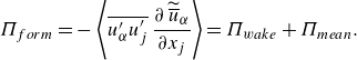 \begin{equation} \Pi _{{form}} = - \left \langle { \overline {u^{\prime}_\alpha u^{\prime}_j} } \, \frac { \partial \, \widetilde { \overline {u} }_\alpha }{ \partial x_j } \right \rangle = \Pi _{{wake}} + \Pi _{{mean}}. \end{equation}
As shown by (2.10), the form-induced production represents the work that the local Reynolds stresses perform against local gradients due to spatial velocity variations.
2.5. Budget equation for the WKE components
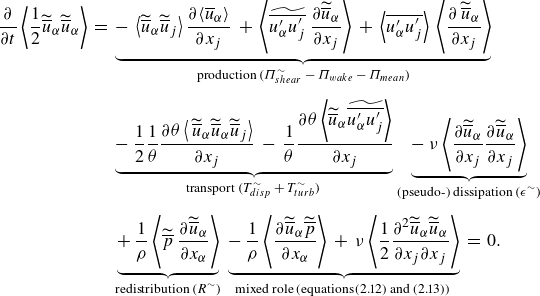
Similarly, it is possible to formulate budget equations for the dispersive normal stresses. Again, no summation over index $\alpha =1,2,3$
is intended if one wishes to obtain the budgets for the three individual components of the WKE, separately. To ensure a clear distinction from terms of the TKE budget, we add the superscript
$\alpha =1,2,3$
is intended if one wishes to obtain the budgets for the three individual components of the WKE, separately. To ensure a clear distinction from terms of the TKE budget, we add the superscript $\,^\sim$
to terms of the WKE budget, such that
$\,^\sim$
to terms of the WKE budget, such that
 \begin{align} \frac {\partial }{\partial t} \left \langle \frac {1}{2} \widetilde {\overline {u}}_\alpha \widetilde {\overline {u}}_\alpha \right \rangle \: = \: & \underbrace { - \: \left \langle \widetilde {\overline {u}}_\alpha \widetilde {\overline {u}}_j \right \rangle \frac {\partial \langle \overline {u}_\alpha \rangle }{\partial x_j} \: + \: \left \langle \widetilde {\overline {u_\alpha ' u_j'}} \, \frac { \partial \widetilde {\overline {u}}_\alpha }{\partial x_j} \right \rangle \: + \: \left \langle \overline {u^{\prime}_\alpha u^{\prime}_j} \right \rangle \, \left \langle \frac { \partial \, \widetilde { \overline {u} }_\alpha }{ \partial x_j } \right \rangle }_{ \text{ production $( \Pi _{shear}^\sim - \Pi _{wake} - \Pi _{mean} )$ } } \nonumber\\[5pt] & \underbrace { - \: \frac {1}{2} \frac {1}{\theta } \frac {\partial \theta \left \langle \, \widetilde {\overline {u}}_\alpha \widetilde {\overline {u}}_\alpha \widetilde {\overline {u}}_j \right \rangle }{\partial x_j} \: - \: \frac {1}{\theta } \frac { \partial \theta \left \langle \widetilde {\overline {u}}_\alpha \widetilde {\overline {u_\alpha ' u_j'}} \right \rangle }{\partial x_j} }_{\text{transport $( T_{disp}^\sim + T_{turb}^\sim )$ }} \underbrace { - \: \nu \left \langle \frac {\partial \widetilde {\overline {u}}_\alpha }{\partial x_j} \frac {\partial \widetilde {\overline {u}}_\alpha }{\partial x_j} \right \rangle }_{\text{(pseudo-) dissipation $( \epsilon ^\sim )$}}\nonumber \\[5pt] & \underbrace { + \: \frac {1}{\rho } \left \langle \widetilde {\overline {p}} \: \frac {\partial \widetilde {\overline {u}}_\alpha }{\partial x_\alpha } \right \rangle }_{\text{redistribution $( R^\sim )$}} \: \underbrace { - \: \frac {1}{\rho } \left \langle \frac {\partial \widetilde {\overline {u}}_\alpha \widetilde {\overline {p}} }{\partial x_\alpha } \right \rangle \: + \: \nu \left \langle \frac {1}{2} \frac {\partial ^2 \widetilde {\overline {u}}_\alpha \widetilde {\overline {u}}_\alpha }{\partial x_j \partial x_j} \right \rangle }_{\text{mixed role (equations (2.12) and (2.13)) }} {\: = \: 0}. \end{align}
The first term on the right-hand side of (2.11) represents a shear production mechanism, as dispersive shear stresses act against the bed-normal gradient of the double-averaged flow velocity. The second and third terms resemble the wake and mean production, respectively, which we summarise as form-induced production. Compared with (2.9), the terms appear here with opposite sign. The fourth and fifth terms are responsible for dispersive and turbulent transport in bed-normal direction, as the terms can only have non-zero values for $j=3$
. The sixth and seventh terms are identified as dissipation and inter-component redistribution of spatial variance, respectively. The last two terms on the right-hand side of (2.11) remind of pressure diffusion and viscous transport. A mere interpretation as transport terms, however, would neglect the non-zero boundary terms
$j=3$
. The sixth and seventh terms are identified as dissipation and inter-component redistribution of spatial variance, respectively. The last two terms on the right-hand side of (2.11) remind of pressure diffusion and viscous transport. A mere interpretation as transport terms, however, would neglect the non-zero boundary terms $BT_\alpha ( \widetilde {\overline {u}}_\alpha \widetilde {\overline {p}})/\rho$
and
$BT_\alpha ( \widetilde {\overline {u}}_\alpha \widetilde {\overline {p}})/\rho$
and $BT_j ( \nu \, \widetilde {\overline {u}}_\alpha \, \partial \widetilde {\overline {u}}_\alpha / \partial x_j )$
. These boundary terms could be interpreted as transport of
$BT_j ( \nu \, \widetilde {\overline {u}}_\alpha \, \partial \widetilde {\overline {u}}_\alpha / \partial x_j )$
. These boundary terms could be interpreted as transport of $\widetilde {\overline {u}}_\alpha \widetilde {\overline {u}}_\alpha$
across the fluid–solid interface, which is formally possible as both
$\widetilde {\overline {u}}_\alpha \widetilde {\overline {u}}_\alpha$
across the fluid–solid interface, which is formally possible as both $\widetilde {\overline {u}}_\alpha$
and
$\widetilde {\overline {u}}_\alpha$
and $\langle \overline {u}_\alpha \rangle$
violate the no-slip boundary condition. Knowing that the boundary term represents an integral along the intersection curve
$\langle \overline {u}_\alpha \rangle$
violate the no-slip boundary condition. Knowing that the boundary term represents an integral along the intersection curve $s$
of the averaging plane with the solid sphere surfaces (see (2.6)), we can substitute
$s$
of the averaging plane with the solid sphere surfaces (see (2.6)), we can substitute $\widetilde {\overline {u}}_\alpha = - \langle \overline {u}_\alpha \rangle$
due to the no-slip boundary condition on the sphere surfaces, and we obtain
$\widetilde {\overline {u}}_\alpha = - \langle \overline {u}_\alpha \rangle$
due to the no-slip boundary condition on the sphere surfaces, and we obtain
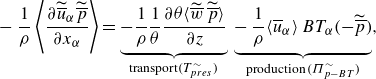 \begin{align}&\quad - \frac {1}{\rho } \left \langle \frac {\partial \widetilde {\overline {u}}_\alpha \widetilde {\overline {p {}}} }{\partial x_\alpha } \right \rangle = \underbrace { - \frac {1}{\rho } \frac {1}{\theta } \frac {\partial \theta \langle \widetilde {\overline {w}} \: \widetilde {\overline {p}} \rangle }{\partial z} }_{{\textrm {transport} ( T_{pres}^\sim )}} \, \underbrace { - \, \frac {1}{\rho } \langle \overline {u}_\alpha \rangle \: BT_\alpha ( -\widetilde {\overline {p}} ) }_{{\textrm {production}} \: ( \Pi _{p{-BT}}^\sim )}, \end{align}
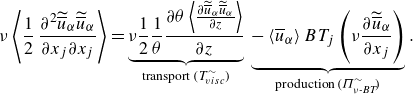 \begin{align}& \nu \left \langle \frac {1}{2} \: \frac {\partial ^2 \widetilde {\overline {u}}_\alpha \widetilde {\overline {u}}_\alpha }{\partial x_j \partial x_j} \right \rangle = \underbrace { \nu \frac {1}{2} \frac {1}{\theta } \frac { \partial \theta \left \langle \frac { \partial \widetilde {\overline {u}}_\alpha \widetilde {\overline {u}}_\alpha }{ \partial z} \right \rangle }{ \partial z } }_{\text{transport $( T_{visc}^\sim )$}} \, \underbrace { - \, \langle \overline {u}_\alpha \rangle \: BT_j \left ( \nu \frac { \partial \widetilde {\overline {u}}_\alpha }{ \partial x_j} \right ) }_{\text{production} \: ( \Pi _{\nu \textit{-BT}}^\sim )} . \end{align}
The formulation in (2.12) and (2.13) isolates exclusive bed-normal transport terms $T_{{pres}}^\sim$
and
$T_{{pres}}^\sim$
and $T_{{visc}}^\sim$
from fluxes across the fluid solid interface, which appear as the production terms
$T_{{visc}}^\sim$
from fluxes across the fluid solid interface, which appear as the production terms $\Pi _{p\textit{-BT}}^\sim$
and
$\Pi _{p\textit{-BT}}^\sim$
and $\Pi _{\nu \textit{-BT}}^\sim$
. The formulation suggests that spatial variance is generated as the double-averaged bed-parallel velocities work against the pressure drag and the part of the viscous drag that results from in-plane velocity variations. For the pressure drag, it can be shown that
$\Pi _{\nu \textit{-BT}}^\sim$
. The formulation suggests that spatial variance is generated as the double-averaged bed-parallel velocities work against the pressure drag and the part of the viscous drag that results from in-plane velocity variations. For the pressure drag, it can be shown that $BT_\alpha (\widetilde { \overline {p} }) = BT_\alpha ( \overline {p} )$
for
$BT_\alpha (\widetilde { \overline {p} }) = BT_\alpha ( \overline {p} )$
for $\alpha = 1,2$
, such that it makes no practical difference whether
$\alpha = 1,2$
, such that it makes no practical difference whether $\langle \overline {p} \rangle$
is included if
$\langle \overline {p} \rangle$
is included if $\langle \overline {w} \rangle = 0$
. However, it appears plausible that the viscous drag component
$\langle \overline {w} \rangle = 0$
. However, it appears plausible that the viscous drag component $\langle \overline {u}_\alpha \rangle \: BT_j ( \partial \langle \overline {u}_\alpha \rangle / \partial x_j )$
does not contribute to the production of WKE, as otherwise, spatial variances would also be spuriously introduced into the flow over a horizontal and smooth surface. Whereas WKE production due to pressure drag is well documented (e.g. Raupach & Shaw Reference Raupach and Shaw1982), the WKE production due to viscous interaction with solid surfaces is often neglected in budget formulations (e.g. Raupach & Shaw Reference Raupach and Shaw1982; Yuan & Piomelli Reference Yuan and Piomelli2014; Ghodke & Apte Reference Ghodke and Apte2016; Hantsis & Piomelli Reference Hantsis and Piomelli2020). The fact that viscous surface interactions can lead to spatial variance in an otherwise undisturbed velocity field is illustrated by figure 1, where boundary layers form on both sides of a very thin plate, which pierces the
$\langle \overline {u}_\alpha \rangle \: BT_j ( \partial \langle \overline {u}_\alpha \rangle / \partial x_j )$
does not contribute to the production of WKE, as otherwise, spatial variances would also be spuriously introduced into the flow over a horizontal and smooth surface. Whereas WKE production due to pressure drag is well documented (e.g. Raupach & Shaw Reference Raupach and Shaw1982), the WKE production due to viscous interaction with solid surfaces is often neglected in budget formulations (e.g. Raupach & Shaw Reference Raupach and Shaw1982; Yuan & Piomelli Reference Yuan and Piomelli2014; Ghodke & Apte Reference Ghodke and Apte2016; Hantsis & Piomelli Reference Hantsis and Piomelli2020). The fact that viscous surface interactions can lead to spatial variance in an otherwise undisturbed velocity field is illustrated by figure 1, where boundary layers form on both sides of a very thin plate, which pierces the $x$
-
$x$
- $y$
-averaging plane. From a mathematical perspective, the decomposition in (2.13) ensures that the viscous transport
$y$
-averaging plane. From a mathematical perspective, the decomposition in (2.13) ensures that the viscous transport $T_{{visc}}^\sim$
is free of net sources, which is an important property of a transport term.
$T_{{visc}}^\sim$
is free of net sources, which is an important property of a transport term.
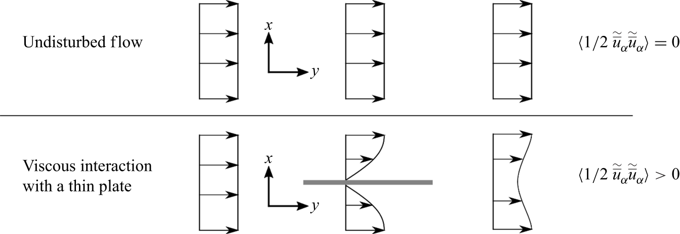
Figure 1. Introduction of spatial variance to the flow field by exclusively viscous interaction on the surface of a very thin plate with flow-parallel orientation. The sketch shows a top view of the averaging plane ( $x$
-
$x$
- $y$
-plane).
$y$
-plane).
2.6. Budget equation for the MKE
From multiplying (2.7) with $\left \langle \overline {u} \right \rangle$
, we obtain the MKE budget equation for the streamwise velocity component, which completes the set of budget equations. This equation reads
$\left \langle \overline {u} \right \rangle$
, we obtain the MKE budget equation for the streamwise velocity component, which completes the set of budget equations. This equation reads
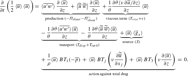 \begin{align} \frac {\partial }{\partial t} \left ( \frac {1}{2} \left \langle \overline {u} \right \rangle \left \langle \overline {u} \right \rangle \right ) = \: & \underbrace { \big \langle \overline {u' w'} \big \rangle \, \frac { \partial \, \langle \overline {u} \rangle }{ \partial z } \: + \: \left \langle \widetilde {\overline {u}} \: \widetilde {\overline {w}} \right \rangle \frac {\partial \langle \overline {u} \rangle }{\partial z } }_{ \text{ production} \ ( - \Pi _{shear} - \Pi _{shear}^\sim ) } \: \underbrace { + \: \frac {1}{\theta } \frac {\partial \theta \langle \nu \, \partial \overline {u} / \partial z \rangle }{\partial z} \: \langle \overline {u} \rangle }_{\text{viscous term}\ ( T_{visc} + \epsilon ) } \nonumber\\[4pt] & \underbrace { - \: \frac {1}{\theta } \frac { \partial \theta \langle \overline {u' w'} \rangle \langle \overline {u} \rangle }{ \partial z } \: - \: \frac {1}{\theta } \frac { \partial \theta \langle \widetilde {\overline {u}} \,\widetilde {\overline {w}} \rangle \langle \overline {u} \rangle }{ \partial z } }_{\text{transport}\ ( T_{disp} + T_{turb} ) } \: \underbrace { + \: \langle \overline {u} \rangle \: \langle \overline {g}_x \rangle }_{\text{source}\ ( S )} \: \nonumber\\[4pt] & \underbrace { + \, \frac {1}{\rho } \langle \overline {u} \rangle \: BT_1(-\overline {p}) \: + \: \langle \overline {u} \rangle \: BT_j\left ( \nu \frac {\partial \widetilde { \overline {u}} }{\partial x_j} \right ) \: + \: \langle \overline {u} \rangle \: BT_3\left ( \nu \frac {\partial \langle \overline {u} \rangle }{\partial z} \right ) }_{\text{ action against total drag }} {\: = \: 0}. \end{align}
The first and second terms on the right-hand side of (2.14) resemble the shear production terms, which appear in (2.9) and (2.11) with the opposite sign. The third term, labelled ‘viscous term’, summarises viscous transport and viscous dissipation, whereas we refrain from a lengthy reformulation of the term, which introduces multiple boundary terms. The fourth and fifth terms can be identified as transport terms. The driving volume force $g_x$
acts as a source of MKE in the sixth term. Altogether, terms seven to nine represent the work of the double-averaged streamwise flow field against the drag. Knowing that
$g_x$
acts as a source of MKE in the sixth term. Altogether, terms seven to nine represent the work of the double-averaged streamwise flow field against the drag. Knowing that $BT_1(\widetilde { \overline {p} }) = BT_1( \overline {p} )$
, we detect that the seventh and eighth term appear here with opposite signs as in (2.12) and (2.13), which is not the case for the ninth term.
$BT_1(\widetilde { \overline {p} }) = BT_1( \overline {p} )$
, we detect that the seventh and eighth term appear here with opposite signs as in (2.12) and (2.13), which is not the case for the ninth term.
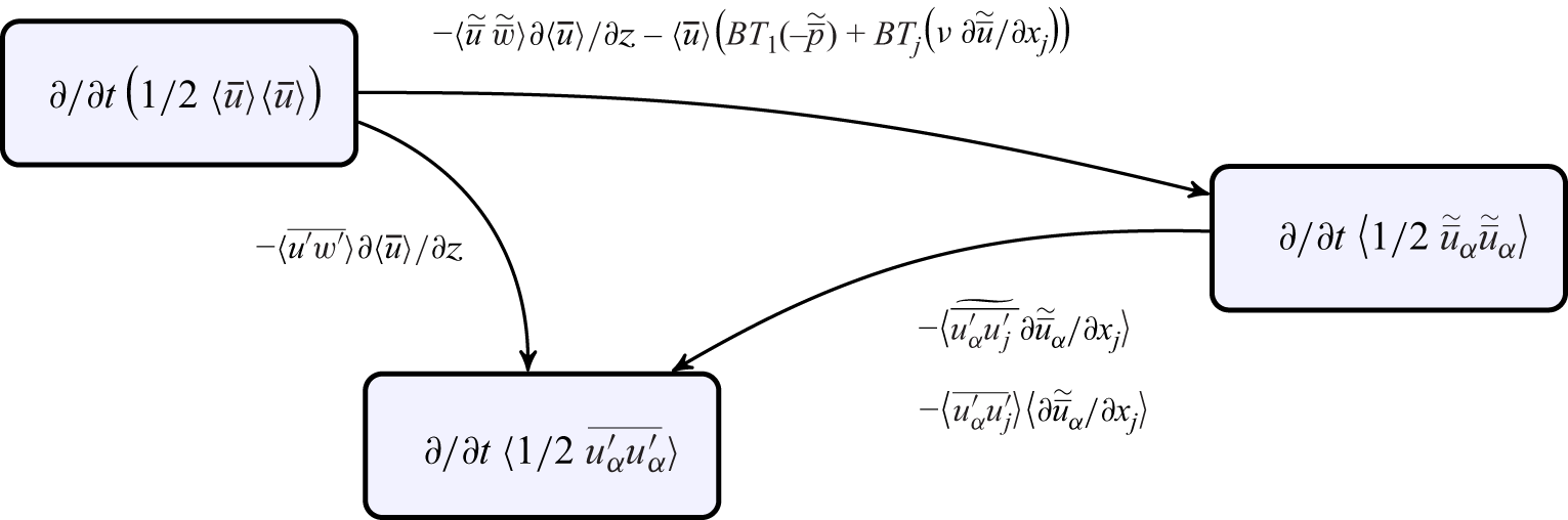
Figure 2. Energy transfer pathways between MKE, WKE and TKE. The arrows indicate the direction of energy flow when the corresponding terms have a positive value. Sources by volume forces, losses by dissipation and vertical transport are not depicted.
2.7. Energy transfer mechanisms
We conclude the theory part by summarising all transfer mechanisms between TKE, WKE and MKE, which are identified by means of terms that appear with opposite signs in the budget equations. Figure 2 visualises the energy transfer pathways between the budgets. The arrows indicate the direction of energy transfer if the corresponding terms have positive values. Transport terms, dissipative losses of WKE and TKE, as well as energy input into the MKE budget due to the volume force are not shown explicitly. According to the energy transfer pathways, shear production mechanisms can generate TKE or WKE at the expense of MKE. Additionally, WKE can result from the work of the double-averaged flow field against the pressure drag and the part of the viscous drag, which is caused by spatial velocity variations. Finally, form-induced production can transfer WKE into TKE and vice versa.
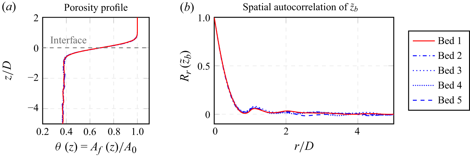
Figure 3. Properties of the sediment bed. (a) In-plane porosity profiles of different realisations of the sphere pack. The interface $z=0$
is defined where
$z=0$
is defined where $\partial ^2 \theta / \partial z^2 = 0$
. The porosity profiles are aligned according to the interface position. (b) Spatial autocorrelation of the bed elevation fluctuation
$\partial ^2 \theta / \partial z^2 = 0$
. The porosity profiles are aligned according to the interface position. (b) Spatial autocorrelation of the bed elevation fluctuation $\tilde {z}_b$
over the horizontal shift
$\tilde {z}_b$
over the horizontal shift $r$
for different realisations.
$r$
for different realisations.
3. Methodology
We have simulated turbulent open-channel flow over mono-disperse random sphere packs (v.Wenczowski & Manhart Reference v. Wenczowski and Manhart2024). In the case configuration, the sphere pack approximates the sediment bed of a gravel bed river, whereas the spheres play the role of sediment grains and remain static during the flow simulation. By fully resolving the pore space, we allow the flow to enter the pore space. The bottom domain boundary intersects the sphere pack. A free-slip condition ensures that momentum is only transferred to the sphere surfaces and not at the bottom wall, which thus reduces the influence of the bottom domain boundary. On the surface of the spheres, a no-slip boundary condition is specified. At the top domain boundary, a free-slip condition is used to approximate a free water surface. In the streamwise $x$
-direction and lateral
$x$
-direction and lateral $y$
-direction, periodic domain boundary conditions are set. A constant volume force in streamwise direction emulates the effect of gravity in a sloped channel. In the statistically stationary state, the flow depth
$y$
-direction, periodic domain boundary conditions are set. A constant volume force in streamwise direction emulates the effect of gravity in a sloped channel. In the statistically stationary state, the flow depth $h$
equals the thickness
$h$
equals the thickness $\delta$
of the fully developed boundary layer.
$\delta$
of the fully developed boundary layer.
3.1. Representation of the porous medium
Mono-disperse random sphere packs of different extents were generated as described by v.Wenczowski & Manhart (Reference v. Wenczowski and Manhart2024). The generation process is conducted such that a level mean bed surface results. Exemplarily, figure 3(a) shows the in-plane porosity profiles $\theta (z)$
of five different realisations of the bed used in the M-cases, which has a base area of
$\theta (z)$
of five different realisations of the bed used in the M-cases, which has a base area of $A_0 = 64D \times 32D$
. The collapse of porosity profiles for different realisations indicates that the generation mechanism avoids strongly unique features. The inflection point
$A_0 = 64D \times 32D$
. The collapse of porosity profiles for different realisations indicates that the generation mechanism avoids strongly unique features. The inflection point $\partial ^2 \theta / \partial z^2 = 0$
of the porosity profile is used as a geometric interface definition, which is consistent with Voermans et al. (Reference Voermans, Ghisalberti and Ivey2017). The distance from the geometrically determined interface to the top domain boundary defines the different flow depths
$\partial ^2 \theta / \partial z^2 = 0$
of the porosity profile is used as a geometric interface definition, which is consistent with Voermans et al. (Reference Voermans, Ghisalberti and Ivey2017). The distance from the geometrically determined interface to the top domain boundary defines the different flow depths $h$
, whereas the sediment bed has a thickness of
$h$
, whereas the sediment bed has a thickness of $5 D$
in all simulated cases. The local bed elevation
$5 D$
in all simulated cases. The local bed elevation $z_b$
is obtained by defining a vertical line at position
$z_b$
is obtained by defining a vertical line at position $(x,y)$
. The height of the topmost intersection point between this line and the surface of the sediment grains yields
$(x,y)$
. The height of the topmost intersection point between this line and the surface of the sediment grains yields $z_b(x,y)$
. The variable
$z_b(x,y)$
. The variable $\tilde {z}_b$
represents the fluctuation of the bed elevation field around its mean value. Figure 3(b) describes the bed surface by means of the spatial autocorrelation of
$\tilde {z}_b$
represents the fluctuation of the bed elevation field around its mean value. Figure 3(b) describes the bed surface by means of the spatial autocorrelation of $\tilde {z}_b$
. A fast decay of the spatial autocorrelation function indicates that no repeating patterns are present in the bed surface.
$\tilde {z}_b$
. A fast decay of the spatial autocorrelation function indicates that no repeating patterns are present in the bed surface.
3.2. Parameter space
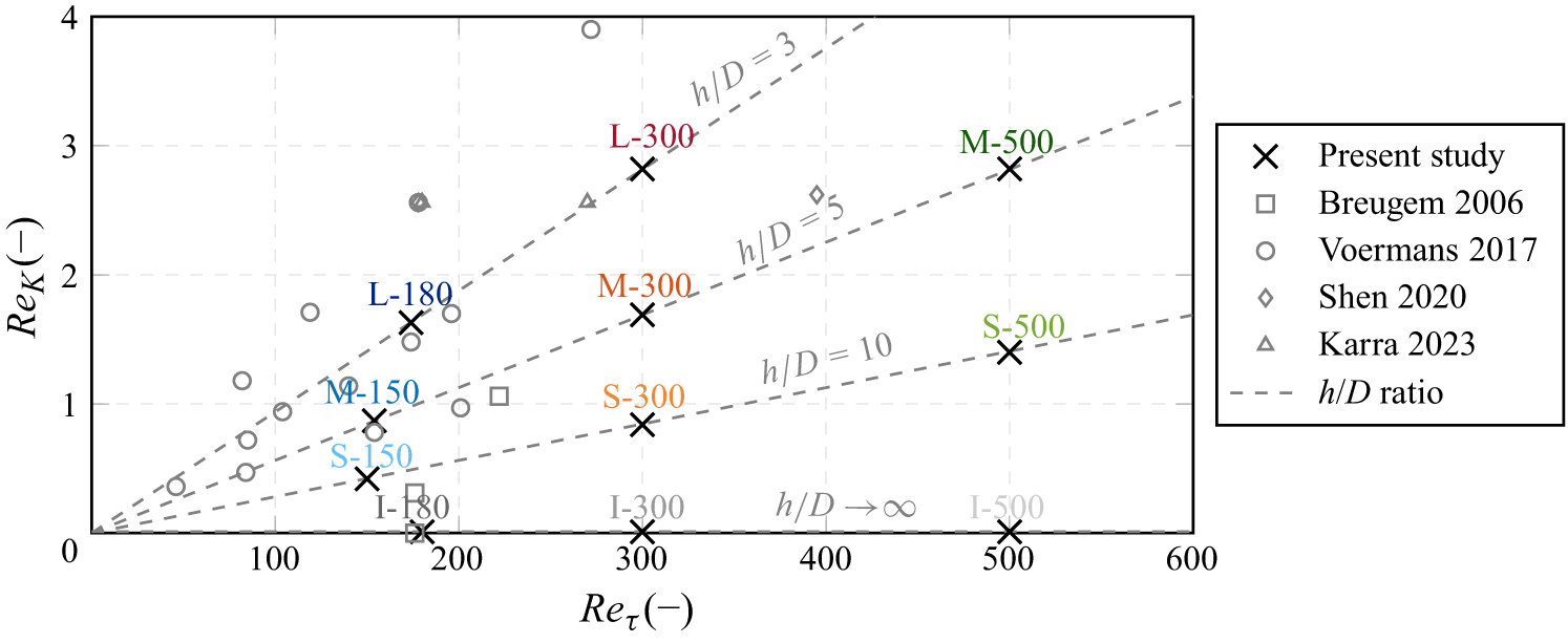
Figure 4. Overview of the dimensionless parameter space, including reference points from the literature. The grey dashed lines represent fixed ratios between the flow depth $h$
(i.e. boundary layer thickness) and the sphere diameter
$h$
(i.e. boundary layer thickness) and the sphere diameter $D$
. As reference points, we refer to Breugem et al. (Reference Breugem, Boersma and Uittenbogaard2006), Voermans et al. (Reference Voermans, Ghisalberti and Ivey2017), Shen et al. (Reference Shen, Yuan and Phanikumar2020) and Karra et al. (Reference Karra, Apte, He and Scheibe2023). Figure adapted from v.Wenczowski & Manhart (Reference v. Wenczowski and Manhart2024).
$D$
. As reference points, we refer to Breugem et al. (Reference Breugem, Boersma and Uittenbogaard2006), Voermans et al. (Reference Voermans, Ghisalberti and Ivey2017), Shen et al. (Reference Shen, Yuan and Phanikumar2020) and Karra et al. (Reference Karra, Apte, He and Scheibe2023). Figure adapted from v.Wenczowski & Manhart (Reference v. Wenczowski and Manhart2024).
Various Reynolds numbers can be used to characterise the flow conditions in different regions of the domain (e.g. Voermans et al. Reference Voermans, Ghisalberti and Ivey2017). We choose the friction Reynolds number $Re_\tau$
and permeability Reynolds number
$Re_\tau$
and permeability Reynolds number $Re_K$
as the primary parameters to span a two-dimensional parameter space. The friction Reynolds number
$Re_K$
as the primary parameters to span a two-dimensional parameter space. The friction Reynolds number $Re_\tau = u_\tau h / \nu$
is well-established in channel flow investigations and describes the unconfined flow above the sediment layer. In contrast, the permeability Reynolds number
$Re_\tau = u_\tau h / \nu$
is well-established in channel flow investigations and describes the unconfined flow above the sediment layer. In contrast, the permeability Reynolds number $Re_K = u_\tau \sqrt {K} / \nu$
characterises the interface of the porous medium. Both Reynolds numbers consider the friction velocity
$Re_K = u_\tau \sqrt {K} / \nu$
characterises the interface of the porous medium. Both Reynolds numbers consider the friction velocity $u_\tau$
, which we compute via a balance of forces as
$u_\tau$
, which we compute via a balance of forces as $u_\tau = \sqrt { g_x h }$
. The permeability Reynolds number uses the square root of the sediment permeability
$u_\tau = \sqrt { g_x h }$
. The permeability Reynolds number uses the square root of the sediment permeability $K$
as a length scale, which can be conceptually understood as an effective pore diameter (Breugem et al. Reference Breugem, Boersma and Uittenbogaard2006). According to the Kozeny–Carman equation (Kozeny Reference Kozeny1927; Carman Reference Carman1937),
$K$
as a length scale, which can be conceptually understood as an effective pore diameter (Breugem et al. Reference Breugem, Boersma and Uittenbogaard2006). According to the Kozeny–Carman equation (Kozeny Reference Kozeny1927; Carman Reference Carman1937), $\sqrt {K}$
is proportional to the sphere diameter
$\sqrt {K}$
is proportional to the sphere diameter $D$
. Relating this length scale to the viscous sublayer length scale,
$D$
. Relating this length scale to the viscous sublayer length scale, $Re_K$
describes if the smallest scales of turbulent motion can penetrate into the pore space. Accordingly,
$Re_K$
describes if the smallest scales of turbulent motion can penetrate into the pore space. Accordingly, $Re_K \ll 1$
and
$Re_K \ll 1$
and $Re_K \gg 1$
indicate effectively impermeable and highly permeable boundaries, respectively, whereas
$Re_K \gg 1$
indicate effectively impermeable and highly permeable boundaries, respectively, whereas $Re_K \approx 1 {-} 2$
is identified as a transition between both extremes (Voermans et al. Reference Voermans, Ghisalberti and Ivey2017). A variation of
$Re_K \approx 1 {-} 2$
is identified as a transition between both extremes (Voermans et al. Reference Voermans, Ghisalberti and Ivey2017). A variation of $h/D$
, i.e. the ratio of the flow depth to the sphere diameter, allows us to investigate different combinations of
$h/D$
, i.e. the ratio of the flow depth to the sphere diameter, allows us to investigate different combinations of $Re_\tau$
and
$Re_\tau$
and $Re_K$
. High values of
$Re_K$
. High values of $h/D$
up to
$h/D$
up to $10$
were chosen to mitigate the blocking effect introduced by individual spheres. By considering
$10$
were chosen to mitigate the blocking effect introduced by individual spheres. By considering $Re_\tau \gt 150$
, we aim to reduce low-Reynolds-number effects, whereas the upper bound of
$Re_\tau \gt 150$
, we aim to reduce low-Reynolds-number effects, whereas the upper bound of $Re_\tau = 500$
is dictated by computational affordability. The chosen range of
$Re_\tau = 500$
is dictated by computational affordability. The chosen range of $Re_K = 0.4 {-} 2.8$
includes the transition region around
$Re_K = 0.4 {-} 2.8$
includes the transition region around $Re_K \approx 1 {-} 2$
. In summary, figure 4 visualises the eight sampling points in terms of
$Re_K \approx 1 {-} 2$
. In summary, figure 4 visualises the eight sampling points in terms of $Re_\tau$
and
$Re_\tau$
and $Re_K$
that we probe in this study. Table 1 contains further parameters describing the simulated cases. Among those parameters,
$Re_K$
that we probe in this study. Table 1 contains further parameters describing the simulated cases. Among those parameters, $k_s^+$
deserves special attention, as it allows us to categorise case S-150 as transitionally rough. With
$k_s^+$
deserves special attention, as it allows us to categorise case S-150 as transitionally rough. With $k_s^+ \approx 50 - 60$
, cases M-150 and S-300 lie near the onset of the fully rough regime (e.g. Kadivar et al. Reference Kadivar, Tormey and McGranaghan2021), while the remaining cases lie within the fully rough regime. As described in v.Wenczowski & Manhart (Reference v. Wenczowski and Manhart2024), the values of
$k_s^+ \approx 50 - 60$
, cases M-150 and S-300 lie near the onset of the fully rough regime (e.g. Kadivar et al. Reference Kadivar, Tormey and McGranaghan2021), while the remaining cases lie within the fully rough regime. As described in v.Wenczowski & Manhart (Reference v. Wenczowski and Manhart2024), the values of $k_s^+$
were determined from the velocity shift
$k_s^+$
were determined from the velocity shift $\Delta u^+$
in relation to a smooth-wall flow case at comparable
$\Delta u^+$
in relation to a smooth-wall flow case at comparable $Re_\tau$
. The smooth-wall cases I-180, I-300, and I-500 are formally characterised by
$Re_\tau$
. The smooth-wall cases I-180, I-300, and I-500 are formally characterised by $h/D \to \infty$
. Figure 5 shows both the velocity shift
$h/D \to \infty$
. Figure 5 shows both the velocity shift $\Delta u^+$
and
$\Delta u^+$
and $k_s^+$
in dependence of
$k_s^+$
in dependence of $Re_K$
.
$Re_K$
.
Table 1. Overview of dimensionless parameters. The variable $D$
represents the sphere diameter,
$D$
represents the sphere diameter, $h$
is the flow depth,
$h$
is the flow depth, $L$
is the extent of the domain,
$L$
is the extent of the domain, $\Delta x_{i,min}^+$
provides the side length of the smallest cubic cells near the interface and
$\Delta x_{i,min}^+$
provides the side length of the smallest cubic cells near the interface and $\Delta x_{i,max}^+$
specifies the side length of the largest cells in the free-flow region. Friction, permeability, bulk, particle and roughness Reynolds numbers are defined as
$\Delta x_{i,max}^+$
specifies the side length of the largest cells in the free-flow region. Friction, permeability, bulk, particle and roughness Reynolds numbers are defined as $Re_\tau = u_\tau h / \nu$
,
$Re_\tau = u_\tau h / \nu$
, $Re_K = u_\tau \sqrt {K} / \nu$
,
$Re_K = u_\tau \sqrt {K} / \nu$
, $Re_b = u_b h / \nu$
,
$Re_b = u_b h / \nu$
, $Re_p = \langle \overline {u} \rangle ^s D / \nu$
and
$Re_p = \langle \overline {u} \rangle ^s D / \nu$
and $k_s^+ = u_\tau k_s / \nu$
. Further,
$k_s^+ = u_\tau k_s / \nu$
. Further, $K$
is the permeability,
$K$
is the permeability, $u_\tau$
represents the shear velocity,
$u_\tau$
represents the shear velocity, $u_b$
is the bulk velocity and
$u_b$
is the bulk velocity and $k_s$
is the equivalent sand-grain roughness height.
$k_s$
is the equivalent sand-grain roughness height.
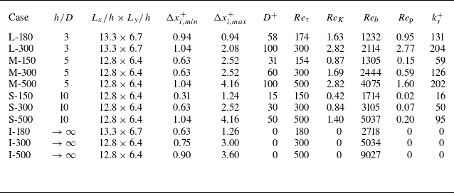
3.3. Interface definition
The nominal parameters of the simulation cases refer to an interface position, which is purely geometrically defined by the inflection point of the porosity profile. In v.Wenczowski & Manhart (Reference v. Wenczowski and Manhart2024), we observed that the drag distribution on the porous medium exhibits a characteristic peak near the sediment–water interface, which marks the region where momentum from the free flow region is absorbed. The features of this characteristic peak were used to describe the interface region. The centroid of the drag distribution was associated with the mean interface position $\mu _z$
, whereas the spread
$\mu _z$
, whereas the spread $\sigma _z$
was found to provide a useful proxy for an interfacial length scale.
$\sigma _z$
was found to provide a useful proxy for an interfacial length scale.
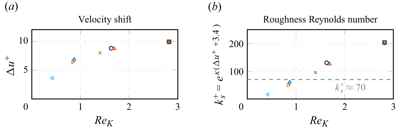
Figure 5. Roughness quantification in dependence of $Re_K$
. (a) Shift
$Re_K$
. (a) Shift $\Delta u^+$
of the velocity profile in comparison to flow over a smooth wall at comparable
$\Delta u^+$
of the velocity profile in comparison to flow over a smooth wall at comparable $Re_\tau$
. (b) Corresponding roughness Reynolds number
$Re_\tau$
. (b) Corresponding roughness Reynolds number $k_s^+$
, computed from
$k_s^+$
, computed from $\Delta u^+$
via the relation given on the y-axis (Jiménez Reference Jiménez2004), where
$\Delta u^+$
via the relation given on the y-axis (Jiménez Reference Jiménez2004), where $\kappa = 0.4$
is used for the von Kármán constant.
$\kappa = 0.4$
is used for the von Kármán constant.
Figure 6 shows the interface parameters $\mu _z$
and
$\mu _z$
and $\sigma _z$
in dependency of
$\sigma _z$
in dependency of $Re_K$
. Whereas the drag-based interface
$Re_K$
. Whereas the drag-based interface $\mu _z$
moves to lower positions with increasing
$\mu _z$
moves to lower positions with increasing $Re_K$
, the spread
$Re_K$
, the spread $\sigma _z / D$
only varies slightly over the
$\sigma _z / D$
only varies slightly over the $Re_K$
-range. In the scope of the present study, positions will be quantified in
$Re_K$
-range. In the scope of the present study, positions will be quantified in $z/D$
, where the vertical coordinate
$z/D$
, where the vertical coordinate $z$
refers to the geometrically defined interface and
$z$
refers to the geometrically defined interface and $D$
is the sphere diameter. Wherever appropriate, we will add the grey dashed line from figure 6(a) to provide the position
$D$
is the sphere diameter. Wherever appropriate, we will add the grey dashed line from figure 6(a) to provide the position $\mu _z$
as a reference.
$\mu _z$
as a reference.
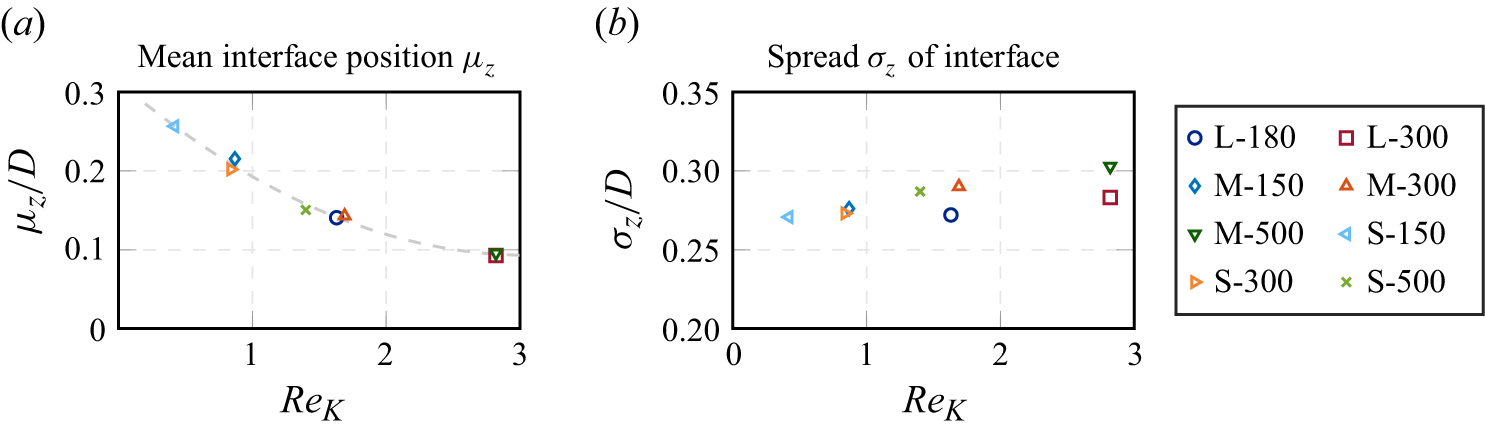
Figure 6. Interface parameters derived from the distribution of drag on the porous medium, as described in v.Wenczowski & Manhart (Reference v. Wenczowski and Manhart2024). The mean interface position $\mu _z$
reflects the drag maximum, whereas
$\mu _z$
reflects the drag maximum, whereas $\sigma _z$
quantifies the spread of the drag distribution.
$\sigma _z$
quantifies the spread of the drag distribution. $D$
represents the sphere diameter.
$D$
represents the sphere diameter.
3.4. Numerical methods
The flow fields were obtained by DNS, for which our in-house code MGLET (Manhart, Tremblay & Friedrich Reference Manhart, Tremblay and Friedrich2001; Manhart Reference Manhart2004; Peller et al. Reference Peller, Duc, Tremblay and Manhart2006; Sakai et al. Reference Sakai, Mendez, Strandenes, Ohlerich, Pasichnyk, Allalen and Manhart2019) was employed. MGLET solves the conservation laws for mass (2.1) and momentum (2.2) by an energy-conserving central second-order finite volume method. A Cartesian grid with staggered arrangement of variables is used with local grid refinement in a multi-level approach (Manhart Reference Manhart2004). An explicit third-order low-storage Runge–Kutta method (Williamson Reference Williamson1980) with a fractional step formulation (Chorin Reference Chorin1967) advances the solution in time. The required pressure update defines an elliptic problem, which is solved efficiently by a multi-level Poisson solver. The geometry of the pore space is resolved by a ghost-cell immersed boundary method, in which a second-order spatial interpolation accuracy is coupled with a correction algorithm to ensure local mass conservation (Peller et al. Reference Peller, Duc, Tremblay and Manhart2006; Peller Reference Peller2010). In Appendix B, we describe the implemented ghost-cell immersed boundary method in detail and show the convergence behaviour of different terms accompanied by a comparison to a body-fitted mesh.
3.5. Accuracy assessment
The convergence of the flow simulation for a random sphere pack was demonstrated in v.Wenczowski & Manhart (Reference v. Wenczowski and Manhart2024), yielding that $48$
cells per diameter are sufficient to obtain an accurate representation of the permeability. Further, a reasonable agreement of the double-averaged velocity profile and the turbulent and dispersive stresses with experimental data of Voermans et al. (Reference Voermans, Ghisalberti and Ivey2017) has been observed. It was also demonstrated that the near-interface spatial resolution of
$48$
cells per diameter are sufficient to obtain an accurate representation of the permeability. Further, a reasonable agreement of the double-averaged velocity profile and the turbulent and dispersive stresses with experimental data of Voermans et al. (Reference Voermans, Ghisalberti and Ivey2017) has been observed. It was also demonstrated that the near-interface spatial resolution of $\Delta x_{i,min}^+ \approx 1.0$
allows an adequate resolution of all turbulent length scales in this region. Statistics were collected over a time
$\Delta x_{i,min}^+ \approx 1.0$
allows an adequate resolution of all turbulent length scales in this region. Statistics were collected over a time $T$
with
$T$
with $T u_\tau / h \in [27, 39]$
.
$T u_\tau / h \in [27, 39]$
.
An evaluation of all terms in the budgets of TKE and WKE allows us to check the closure of the budgets. For the TKE budgets, the largest amplitude of the residual is observed near $z/D \approx 0$
. The residual is smaller than
$z/D \approx 0$
. The residual is smaller than $3\, \%$
of the amplitude of the production peak, which is found at a similar height. In most cases, a positive sign of the residual indicates that we may slightly underpredict the dissipation. In comparison to the TKE, more effort is required to achieve good closure of the WKE budget. Though we exploit the second-order accuracy of the immersed boundary implementation, spikes in the resulting profiles of the term
$3\, \%$
of the amplitude of the production peak, which is found at a similar height. In most cases, a positive sign of the residual indicates that we may slightly underpredict the dissipation. In comparison to the TKE, more effort is required to achieve good closure of the WKE budget. Though we exploit the second-order accuracy of the immersed boundary implementation, spikes in the resulting profiles of the term $\Pi _{\nu \textit{-BT}}^\sim$
near the sphere crests did not vanish. A test with a single sphere (not shown here) allowed us to connect those spikes to the thin viscous boundary layers forming at the crests of individual protruding spheres. For a cleaner graphical representation, however, those spikes were removed by smoothing the profiles with a Gaussian kernel. The smoothed profile for the term
$\Pi _{\nu \textit{-BT}}^\sim$
near the sphere crests did not vanish. A test with a single sphere (not shown here) allowed us to connect those spikes to the thin viscous boundary layers forming at the crests of individual protruding spheres. For a cleaner graphical representation, however, those spikes were removed by smoothing the profiles with a Gaussian kernel. The smoothed profile for the term $\Pi _{\nu \textit{-BT}}^\sim$
keeps the residual in the MKE budget below
$\Pi _{\nu \textit{-BT}}^\sim$
keeps the residual in the MKE budget below $4.2\, \%$
of the production peak.
$4.2\, \%$
of the production peak.
4. Results
In this section, we will first describe the distribution of MKE, WKE and TKE, before we present the budgets for the latter two components of the kinetic energy. Double-averaged profiles as well as the spatial distributions of the kinetic energy components are presented in § 4.1 and § 4.2, respectively. In § 4.3, we investigate the outer-layer behaviour of TKE budget terms, before we focus exclusively on the near-interface region. We discuss one representative near-interface TKE budget in detail (§ 4.4), show the scaling behaviour of source and sink terms (§ 4.5), and decompose the transport into individual processes (§ 4.6). The same analysis steps are repeated for the WKE, such that we start with the near-interface budget (§ 4.7), proceed to the scaling behaviour of sources and sinks (§ 4.8), and finish with a detailed look at the transport (§ 4.9).
4.1. Near-interface profiles of TKE and WKE
As a basis for the discussion of the kinetic energy budgets, figure 7 shows the near-interface profiles of plane-averaged TKE and WKE. The profiles are normalised by $u_\tau$
and plotted against
$u_\tau$
and plotted against $z/D$
.
$z/D$
.
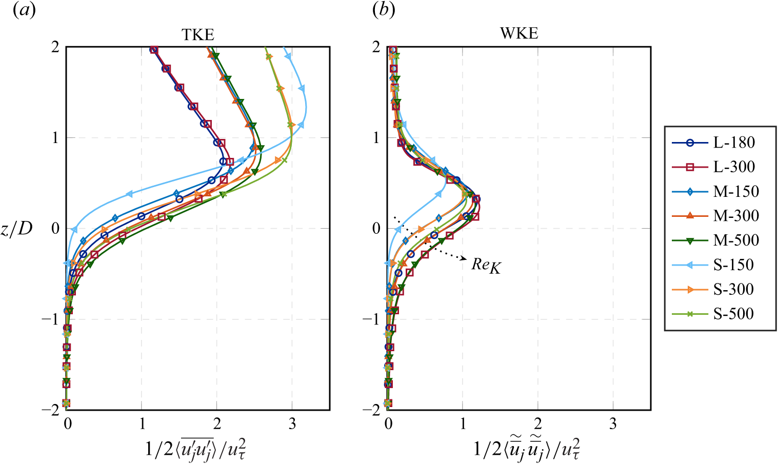
Figure 7. Near-interface profiles of TKE and WKE, normalised by the friction velocity $u_\tau$
. The vertical coordinate
$u_\tau$
. The vertical coordinate $z$
refers to the geometrically defined interface and is normalised by the sphere diameter
$z$
refers to the geometrically defined interface and is normalised by the sphere diameter $D$
.
$D$
.
For all simulated cases, the TKE attains peak values above the interface, and quickly decays near and below the interface. Above their peaks near $z/D \approx 1$
, the TKE profiles group according to the ratio
$z/D \approx 1$
, the TKE profiles group according to the ratio $h/D$
under the given normalisation. A cross-comparison between profiles suggests that both increasing
$h/D$
under the given normalisation. A cross-comparison between profiles suggests that both increasing $Re_\tau$
and increasing
$Re_\tau$
and increasing $Re_K$
contribute to higher intensities of velocity fluctuation at
$Re_K$
contribute to higher intensities of velocity fluctuation at $z/D=0$
. For case S-150, which is associated with the transitionally rough regime, an emphasised peak in the TKE distribution is found at
$z/D=0$
. For case S-150, which is associated with the transitionally rough regime, an emphasised peak in the TKE distribution is found at $z/D \approx 1.2$
, which is above the peak location of other profiles. This qualitative difference of the transitionally rough case S-150 can be explained by the turbulence structure of the buffer layer including streaks and quasi-streamwise vortices, which vanish at higher
$z/D \approx 1.2$
, which is above the peak location of other profiles. This qualitative difference of the transitionally rough case S-150 can be explained by the turbulence structure of the buffer layer including streaks and quasi-streamwise vortices, which vanish at higher $Re_K$
(v.Wenczowski & Manhart Reference v. Wenczowski and Manhart2024). The WKE profiles reach their maxima at
$Re_K$
(v.Wenczowski & Manhart Reference v. Wenczowski and Manhart2024). The WKE profiles reach their maxima at $z/D \approx 0.2 {-} 0.5$
. There is a trend towards higher peaks at lower locations with increasing
$z/D \approx 0.2 {-} 0.5$
. There is a trend towards higher peaks at lower locations with increasing $Re_K$
. Directly above the peak, the WKE decreases rapidly towards the free flow region, such that only small amounts of WKE remain above
$Re_K$
. Directly above the peak, the WKE decreases rapidly towards the free flow region, such that only small amounts of WKE remain above $z/D \approx 1$
. Most profiles behave similarly in the region of
$z/D \approx 1$
. Most profiles behave similarly in the region of $z/D \in [0.5,1]$
near the crests of the topmost spheres, which hints at a direct influence of the bed geometry on the distribution of the WKE. According to the layer concept of Nikora et al. (Reference Nikora, Goring, McEwan and Griffiths2001), which is based on a horizontal-averaging perspective, the nearly complete decay of dispersive stresses at
$z/D \in [0.5,1]$
near the crests of the topmost spheres, which hints at a direct influence of the bed geometry on the distribution of the WKE. According to the layer concept of Nikora et al. (Reference Nikora, Goring, McEwan and Griffiths2001), which is based on a horizontal-averaging perspective, the nearly complete decay of dispersive stresses at $z/D \approx 1.2 - 1.5$
marks the upper end of the form-induced sublayer and, thus, also the upper end of the roughness layer. Below
$z/D \approx 1.2 - 1.5$
marks the upper end of the form-induced sublayer and, thus, also the upper end of the roughness layer. Below $z=0$
, the WKE profiles group well visibly according to
$z=0$
, the WKE profiles group well visibly according to $Re_K$
. With increasing
$Re_K$
. With increasing $Re_K$
, the spatial velocity variations entrain into progressively deeper regions of the sediment. Again, the transitionally rough case S-150 renders an exception, as the amplitude of the WKE peak is smaller and the peak is found at a higher position. This observation can be explained by the rather strong wall-blocking effect at
$Re_K$
, the spatial velocity variations entrain into progressively deeper regions of the sediment. Again, the transitionally rough case S-150 renders an exception, as the amplitude of the WKE peak is smaller and the peak is found at a higher position. This observation can be explained by the rather strong wall-blocking effect at $Re_K \approx 0.4$
, which allows stable recirculation vortices to occupy gaps between the topmost spheres, such that the downstream spheres are sheltered from the approaching flow (v.Wenczowski & Manhart Reference v. Wenczowski and Manhart2024).
$Re_K \approx 0.4$
, which allows stable recirculation vortices to occupy gaps between the topmost spheres, such that the downstream spheres are sheltered from the approaching flow (v.Wenczowski & Manhart Reference v. Wenczowski and Manhart2024).
4.2. Spatial distribution of TKE and WKE
To facilitate the interpretation of the previous profiles, we consider the spatial distributions of $\overline {u_j^\prime u_j^\prime } / 2$
and
$\overline {u_j^\prime u_j^\prime } / 2$
and $\widetilde {\overline {u}}_j \widetilde {\overline {u}}_j / 2$
, i.e. the distribution of the kinetic energies prior to the horizontal averaging operation. Figure 8 visualises the different quantities within a vertical slice through the domain of case M-300. The largest values of the TKE are found slightly above the sediment crests. Between the sediment crests and
$\widetilde {\overline {u}}_j \widetilde {\overline {u}}_j / 2$
, i.e. the distribution of the kinetic energies prior to the horizontal averaging operation. Figure 8 visualises the different quantities within a vertical slice through the domain of case M-300. The largest values of the TKE are found slightly above the sediment crests. Between the sediment crests and $z/D \approx 1.5$
, individual spots of increased TKE are recognisable. The TKE appears to be more homogeneously distributed at larger elevations, suggesting that the influence of spatial inhomogeneities in the sediment bed, such as individual protruding spheres, is limited to a confined region. High values of the WKE are found only in direct proximity of the sediment bed surface. In particular, the wake regions behind the crests of prominently protruding spheres induce strong deviations from the plane-averaged velocity, as shown by the inset in figure 8(b). These regions are likely to be responsible for the peak in the WKE profile, which would also explain the rapid decrease of WKE above the crests of the topmost spheres. The no-slip boundary condition dictates that
$z/D \approx 1.5$
, individual spots of increased TKE are recognisable. The TKE appears to be more homogeneously distributed at larger elevations, suggesting that the influence of spatial inhomogeneities in the sediment bed, such as individual protruding spheres, is limited to a confined region. High values of the WKE are found only in direct proximity of the sediment bed surface. In particular, the wake regions behind the crests of prominently protruding spheres induce strong deviations from the plane-averaged velocity, as shown by the inset in figure 8(b). These regions are likely to be responsible for the peak in the WKE profile, which would also explain the rapid decrease of WKE above the crests of the topmost spheres. The no-slip boundary condition dictates that $\overline {u}_i=0$
on the sphere surface, which implies that
$\overline {u}_i=0$
on the sphere surface, which implies that $\widetilde {\overline {u}}_i = - \langle {\overline {u}}_i \rangle$
. Accordingly, the WKE is generally not zero on the surface of the spheres, but has a local value of
$\widetilde {\overline {u}}_i = - \langle {\overline {u}}_i \rangle$
. Accordingly, the WKE is generally not zero on the surface of the spheres, but has a local value of $\langle {\overline {u}}_j \rangle \langle {\overline {u}}_j \rangle / 2$
, which corresponds to the MKE at the respective
$\langle {\overline {u}}_j \rangle \langle {\overline {u}}_j \rangle / 2$
, which corresponds to the MKE at the respective $z$
-position. As a result, thin layers of large WKE are also found on the wind-ward side of exposed spheres.
$z$
-position. As a result, thin layers of large WKE are also found on the wind-ward side of exposed spheres.
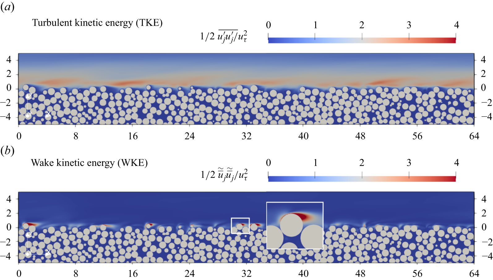
Figure 8. Spatial distribution of TKE and WKE within an arbitrarily chosen $x$
-
$x$
- $z$
-plane of simulation case M-300. The values are normalised by the square of the friction velocity
$z$
-plane of simulation case M-300. The values are normalised by the square of the friction velocity $u_\tau$
. Coordinates in the
$u_\tau$
. Coordinates in the $x$
- and
$x$
- and $z$
-directions are given in
$z$
-directions are given in $x/D$
and
$x/D$
and $z/D$
, respectively, where
$z/D$
, respectively, where $D$
is the sphere diameter.
$D$
is the sphere diameter.
4.3. Outer-layer similarity of TKE budget terms
In v.Wenczowski & Manhart (Reference v. Wenczowski and Manhart2024), we observed an outer-layer similarity among the TKE profiles of cases with comparable $Re_\tau$
. While the TKE profiles far from the sediment surface remained similar across different
$Re_\tau$
. While the TKE profiles far from the sediment surface remained similar across different $h/D$
or
$h/D$
or $Re_K$
, a near-wall TKE peak was damped with increasing
$Re_K$
, a near-wall TKE peak was damped with increasing $Re_K$
. That motivates us to investigate the TKE budgets in an outer scaling with the flow depth
$Re_K$
. That motivates us to investigate the TKE budgets in an outer scaling with the flow depth $h$
and the friction velocity
$h$
and the friction velocity $u_\tau$
. Figure 9 shows the budgets in terms of total production, total transport and dissipation according to (2.9). The profiles are plotted over the complete flow depth, while cases with similar
$u_\tau$
. Figure 9 shows the budgets in terms of total production, total transport and dissipation according to (2.9). The profiles are plotted over the complete flow depth, while cases with similar $Re_\tau$
are shown in one plot. The region far from the surface of the sediment bed is characterised by a collapse of the curves for similar
$Re_\tau$
are shown in one plot. The region far from the surface of the sediment bed is characterised by a collapse of the curves for similar $Re_\tau$
, which suggests an outer-layer similarity of the budget terms. Slightly above the sediment–water interface, the TKE budget terms depend strongly on
$Re_\tau$
, which suggests an outer-layer similarity of the budget terms. Slightly above the sediment–water interface, the TKE budget terms depend strongly on $Re_K$
. Smooth-wall cases and cases with a low permeability Reynolds number show an emphasised production peak in this region, which flattens out with progressively higher
$Re_K$
. Smooth-wall cases and cases with a low permeability Reynolds number show an emphasised production peak in this region, which flattens out with progressively higher $Re_K$
. As the influence of roughness and permeability seems to be most emphasised in the near-interface region, we will focus on this region in a deeper analysis of the budget.
$Re_K$
. As the influence of roughness and permeability seems to be most emphasised in the near-interface region, we will focus on this region in a deeper analysis of the budget.
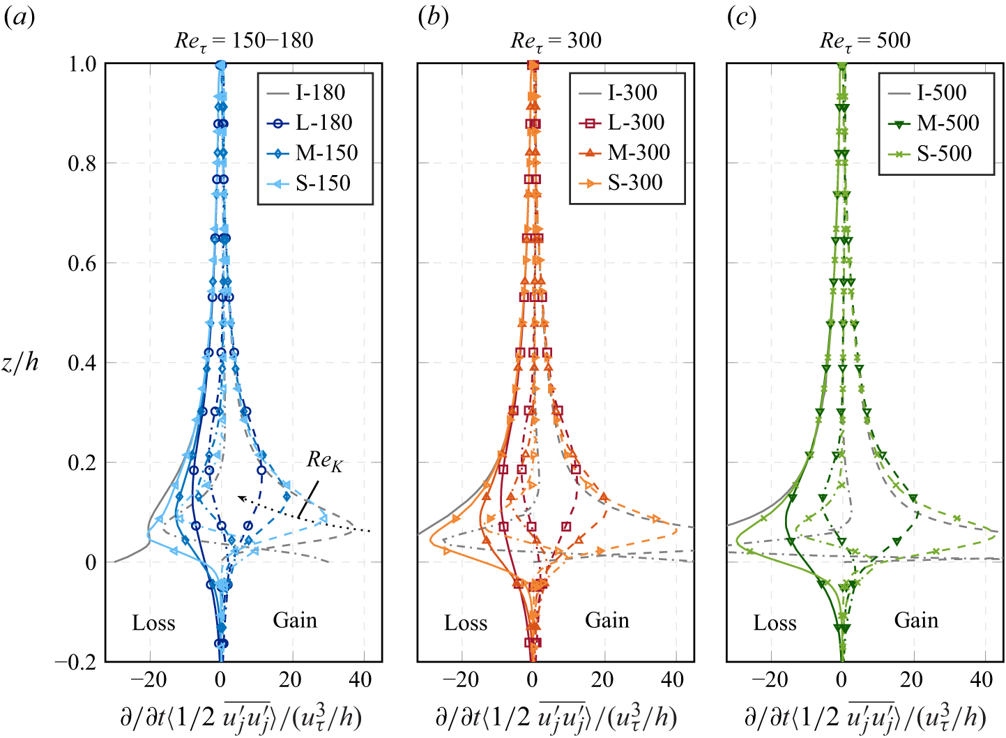
Figure 9. TKE budget terms in outer scaling. Total production ( $\Pi _{\textit{tot}}$
,
$\Pi _{\textit{tot}}$
, ![]() ), total transport (
), total transport ( $T_{\textit{tot}}$
,
$T_{\textit{tot}}$
, ![]() ) and dissipation (
) and dissipation ( $\epsilon$
,
$\epsilon$
, ![]() ) are normalised by the flow depth
) are normalised by the flow depth $h$
and the friction velocity
$h$
and the friction velocity $u_\tau$
. Plots show groups of cases with similar
$u_\tau$
. Plots show groups of cases with similar $Re_\tau$
, but different
$Re_\tau$
, but different $Re_K$
.
$Re_K$
.
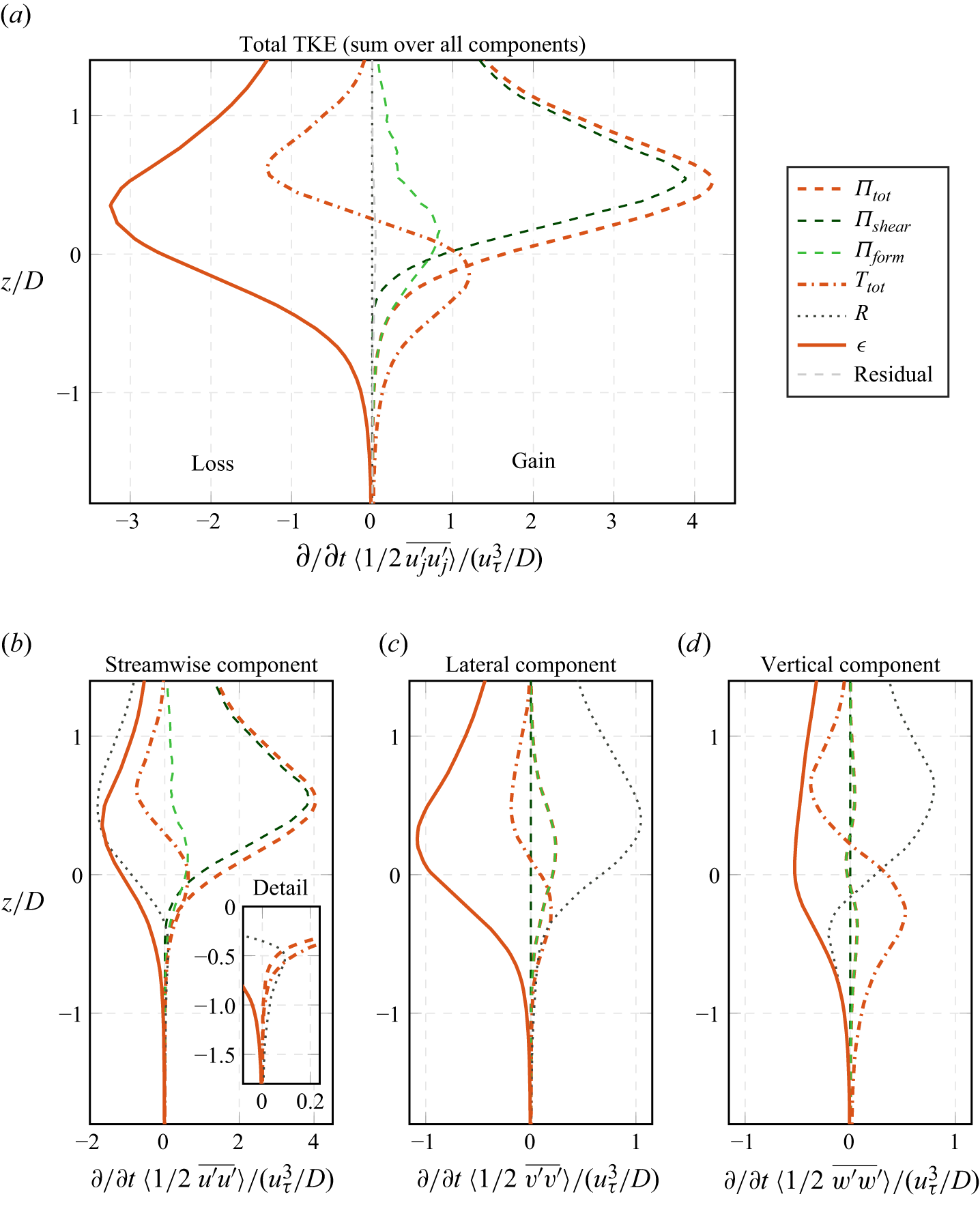
Figure 10. Budgets for the complete TKE and for the individual Reynolds normal stresses in the near-interface region. Case M-300 serves as an example. For normalisation, the shear velocity $u_\tau$
and the sphere diameter
$u_\tau$
and the sphere diameter $D$
are used. The vertical coordinate
$D$
are used. The vertical coordinate $z$
refers to the geometrically defined interface and is normalised by
$z$
refers to the geometrically defined interface and is normalised by $D$
. Note that the horizontal axes cover different value ranges.
$D$
. Note that the horizontal axes cover different value ranges.
4.4. Overview of the near-interface TKE budget
To obtain a comprehensive image of all processes involved, we analyse the near-interface TKE budget of the case M-300. With $Re_\tau = 300$
and
$Re_\tau = 300$
and $Re_K \approx 1.7$
, case M-300 lies approximately in the centre of our parameter space and, thus, provides a representative example. Figure 10(a) shows the TKE budget normalised with the friction velocity
$Re_K \approx 1.7$
, case M-300 lies approximately in the centre of our parameter space and, thus, provides a representative example. Figure 10(a) shows the TKE budget normalised with the friction velocity $u_\tau$
and the sphere diameter
$u_\tau$
and the sphere diameter $D$
, which provides a typical length scale in the interface region. Whereas transport processes are summarised in the total transport
$D$
, which provides a typical length scale in the interface region. Whereas transport processes are summarised in the total transport $T_{\textit{tot}}$
, the individual contributions of shear and form-induced production are plotted separately. The total production peaks at
$T_{\textit{tot}}$
, the individual contributions of shear and form-induced production are plotted separately. The total production peaks at $z/D \approx 0.5$
, whereas the dissipation rate
$z/D \approx 0.5$
, whereas the dissipation rate $\epsilon$
at the same position is smaller. A larger share of the TKE which is produced but not dissipated appears to be transported downwards into the pore space of the porous medium. In the region below
$\epsilon$
at the same position is smaller. A larger share of the TKE which is produced but not dissipated appears to be transported downwards into the pore space of the porous medium. In the region below $z/D \approx -0.1$
, more TKE is provided by the transport than by the production. With increasing depth, the TKE input from transport is nearly exclusively balanced by the dissipation
$z/D \approx -0.1$
, more TKE is provided by the transport than by the production. With increasing depth, the TKE input from transport is nearly exclusively balanced by the dissipation $\epsilon$
. The major part of the TKE production results from shear production, which also seems to determine the position of the production peak. In comparison to that, the contribution of form-induced production appears to be minor, except in the region below
$\epsilon$
. The major part of the TKE production results from shear production, which also seems to determine the position of the production peak. In comparison to that, the contribution of form-induced production appears to be minor, except in the region below $z/D = -0.3$
, where hardly any shear production takes place.
$z/D = -0.3$
, where hardly any shear production takes place.
Figure 10(b–d) provides the budgets for individual components of the TKE. Nearly the complete TKE is produced in the component $\langle \overline {u^\prime u^\prime } \rangle$
. Approximately half of the produced
$\langle \overline {u^\prime u^\prime } \rangle$
. Approximately half of the produced $\langle \overline {u^\prime u^\prime } \rangle$
is dissipated, whereas the rest is redistributed to
$\langle \overline {u^\prime u^\prime } \rangle$
is dissipated, whereas the rest is redistributed to $\langle \overline {v^\prime v^\prime } \rangle$
and
$\langle \overline {v^\prime v^\prime } \rangle$
and $\langle \overline {w^\prime w^\prime } \rangle$
by the pressure redistribution
$\langle \overline {w^\prime w^\prime } \rangle$
by the pressure redistribution $P_{{redist}}$
. The pressure-based inter-component redistribution is the main source of bed-normal velocity fluctuations, and reaches its largest positive contribution in the budget of
$P_{{redist}}$
. The pressure-based inter-component redistribution is the main source of bed-normal velocity fluctuations, and reaches its largest positive contribution in the budget of $\langle \overline {w^\prime w^\prime } \rangle$
at
$\langle \overline {w^\prime w^\prime } \rangle$
at $z/D \approx 0.5$
. Compared with other terms involved, vertical transport plays a major role in the budget of
$z/D \approx 0.5$
. Compared with other terms involved, vertical transport plays a major role in the budget of $\langle \overline {w^\prime w^\prime } \rangle$
. Below a depth of
$\langle \overline {w^\prime w^\prime } \rangle$
. Below a depth of $z/D \lesssim -0.2$
, the pressure-based redistribution term in the budget of
$z/D \lesssim -0.2$
, the pressure-based redistribution term in the budget of $\langle \overline {w^\prime w^\prime } \rangle$
changes its sign, such that TKE is distributed back to the other components. The detail in figure 10(b) shows that this inter-component redistribution even acts as a source of streamwise velocity fluctuations in the region
$\langle \overline {w^\prime w^\prime } \rangle$
changes its sign, such that TKE is distributed back to the other components. The detail in figure 10(b) shows that this inter-component redistribution even acts as a source of streamwise velocity fluctuations in the region $z/D \lt -0.3$
.
$z/D \lt -0.3$
.
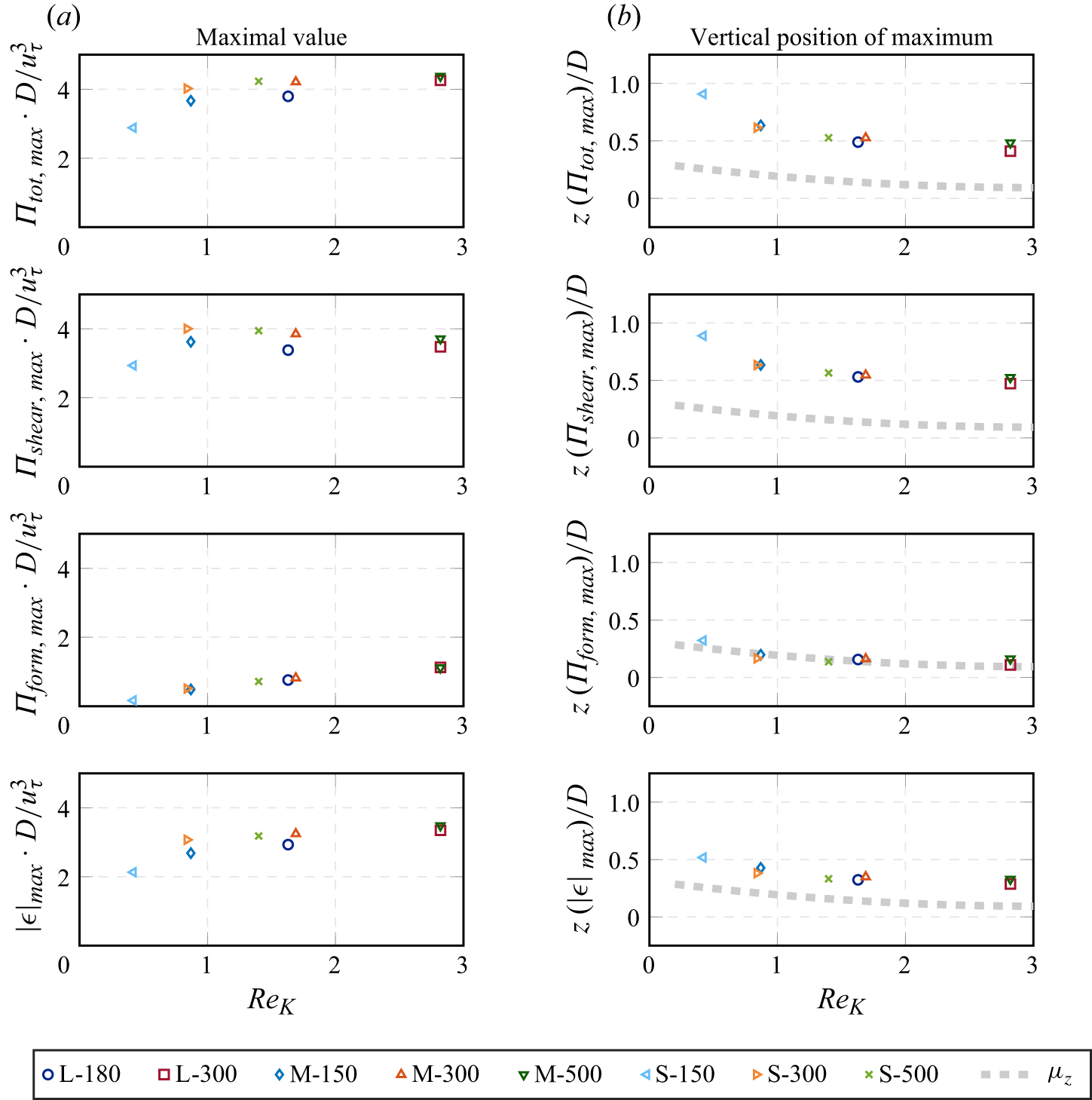
Figure 11. Scaling of production terms and dissipation of TKE with $Re_K$
. (a) Maxima of the processes normalised by the friction velocity
$Re_K$
. (a) Maxima of the processes normalised by the friction velocity $u_\tau$
and the sphere diameter
$u_\tau$
and the sphere diameter $D$
. (b) Vertical position of the maxima with respect to the geometrically defined interface, whereas
$D$
. (b) Vertical position of the maxima with respect to the geometrically defined interface, whereas $z$
is normalised by
$z$
is normalised by $D$
. The grey dashed line represents the position
$D$
. The grey dashed line represents the position $\mu _z$
of the drag-based interface (v.Wenczowski & Manhart Reference v. Wenczowski and Manhart2024). The total production
$\mu _z$
of the drag-based interface (v.Wenczowski & Manhart Reference v. Wenczowski and Manhart2024). The total production $\Pi _{\textit{tot}}$
summarises the shear production
$\Pi _{\textit{tot}}$
summarises the shear production $\Pi _{shear}$
and the form-induced production
$\Pi _{shear}$
and the form-induced production $\Pi _{\textit{form}}$
.
$\Pi _{\textit{form}}$
. $\epsilon$
represents the dissipation.
$\epsilon$
represents the dissipation.
4.5. Scaling of TKE sources and sinks
In what follows, we investigate how the maxima of the production and dissipation and their locations depend on the Reynolds numbers. The left column, i.e. figure 11(a), shows the maximal values normalised with $u_\tau ^3/D$
over
$u_\tau ^3/D$
over $Re_K$
. Figure 11(b) shows the elevations at which the maximum intensity of the respective process is observed. We also added as a reference the position of the centroid of the drag distribution
$Re_K$
. Figure 11(b) shows the elevations at which the maximum intensity of the respective process is observed. We also added as a reference the position of the centroid of the drag distribution $\mu _z$
, which can be used as an interface position (see § 3.3). The normalised total TKE production increases with
$\mu _z$
, which can be used as an interface position (see § 3.3). The normalised total TKE production increases with $Re_K$
, but seems to saturate once the hydraulically fully rough regime is reached (
$Re_K$
, but seems to saturate once the hydraulically fully rough regime is reached ( $k_s^+ \gtrsim 70$
at
$k_s^+ \gtrsim 70$
at $Re_K \gtrsim 1$
). Following the trend of
$Re_K \gtrsim 1$
). Following the trend of $\mu _z$
, the location of the total production peak lowers in the range of
$\mu _z$
, the location of the total production peak lowers in the range of $Re_K \lt 1.5$
, but seems to stabilise at
$Re_K \lt 1.5$
, but seems to stabilise at $z/D \approx 0.5$
for
$z/D \approx 0.5$
for $Re_K \gt 1.5$
. Both in terms of magnitude and position, the peaks of the shear production
$Re_K \gt 1.5$
. Both in terms of magnitude and position, the peaks of the shear production $\Pi _{{shear}}$
appear to go in line with the peaks of total production, as the shear production is the main TKE production mechanism (compare figure 10). The data points of cases L-300 and M-500, however, indicate that higher
$\Pi _{{shear}}$
appear to go in line with the peaks of total production, as the shear production is the main TKE production mechanism (compare figure 10). The data points of cases L-300 and M-500, however, indicate that higher $Re_K$
may also slightly reduce the shear production. Starting from nearly zero-value at
$Re_K$
may also slightly reduce the shear production. Starting from nearly zero-value at $Re_K = 0.42$
, the maximal value of the form-induced production
$Re_K = 0.42$
, the maximal value of the form-induced production $\Pi _{{form}}$
increases monotonously with increasing
$\Pi _{{form}}$
increases monotonously with increasing $Re_K$
. In comparison to
$Re_K$
. In comparison to $\Pi _{shear}$
, however, the form-induced production plays a secondary role. Even at
$\Pi _{shear}$
, however, the form-induced production plays a secondary role. Even at $Re_K \approx 2.8$
, the maximum value of form-induced production is approximately a fourth of the maximal value of shear production. The peak of the form-induced production is found near
$Re_K \approx 2.8$
, the maximum value of form-induced production is approximately a fourth of the maximal value of shear production. The peak of the form-induced production is found near $z=\mu _z$
and, thus, at a lower position than the shear production peak. By means of an instantaneous field, figure 12 illustrates the nature of the form-induced production mechanism. The wake regions behind individual spheres seem to have major contributions. Horseshoe-like vortices, which form on the windward side of exposed spheres, can equally lead to a positive form-induced production. The observation that form-induced production acts on small spatial scales comparable to the grain scale is likely to explain the smaller peak value of
$z=\mu _z$
and, thus, at a lower position than the shear production peak. By means of an instantaneous field, figure 12 illustrates the nature of the form-induced production mechanism. The wake regions behind individual spheres seem to have major contributions. Horseshoe-like vortices, which form on the windward side of exposed spheres, can equally lead to a positive form-induced production. The observation that form-induced production acts on small spatial scales comparable to the grain scale is likely to explain the smaller peak value of $\Pi _{{form}}$
. The maximal amplitude of the dissipation is lower than the maximal values of production, as the dissipation takes place over a wider vertical region than the production. With increasing
$\Pi _{{form}}$
. The maximal amplitude of the dissipation is lower than the maximal values of production, as the dissipation takes place over a wider vertical region than the production. With increasing $Re_K$
, the maximal dissipation values still grow slightly. The dissipation maxima are also found at a lower elevation than the total production maxima, which results from increasing vertical TKE transport into the negative
$Re_K$
, the maximal dissipation values still grow slightly. The dissipation maxima are also found at a lower elevation than the total production maxima, which results from increasing vertical TKE transport into the negative $z$
-direction.
$z$
-direction.
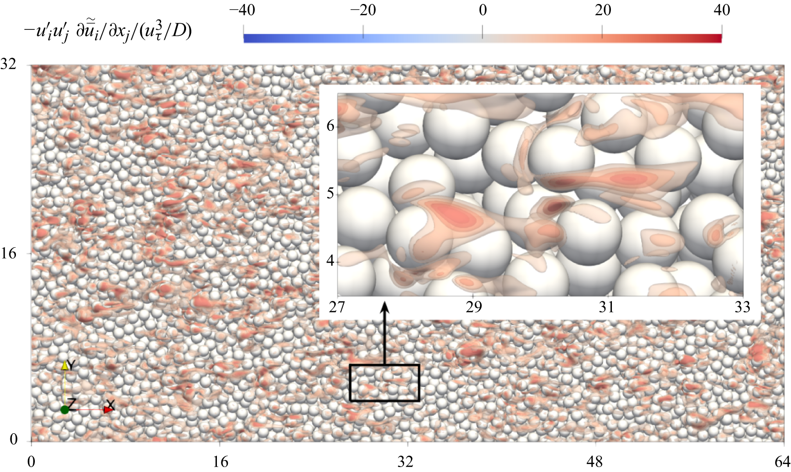
Figure 12. Instantaneous field of the form-induced TKE production mechanism. The shear velocity $u_\tau$
and the sphere diameter
$u_\tau$
and the sphere diameter $D$
are used for normalisation. The shown patch is a fraction of the domain of case M-300. Coordinates are given as
$D$
are used for normalisation. The shown patch is a fraction of the domain of case M-300. Coordinates are given as $x/D$
and
$x/D$
and $y/D$
, respectively.
$y/D$
, respectively.
The observations in figure 11 suggest that the permeability Reynolds number $Re_K$
has decisive impact on the TKE sources and sinks in the interface region, whereas an influence of
$Re_K$
has decisive impact on the TKE sources and sinks in the interface region, whereas an influence of $Re_\tau$
is hardly noticeable. With larger
$Re_\tau$
is hardly noticeable. With larger $Re_K$
, the maxima of different processes move to progressively lower elevations, thus following the drag-based interface (grey dashed lines in figure 11). For
$Re_K$
, the maxima of different processes move to progressively lower elevations, thus following the drag-based interface (grey dashed lines in figure 11). For $Re_K \leq 3$
, shear production remains the dominant production process. In § 5, we discuss the behaviour of the dominant shear production in detail and show how its distribution is linked to the interface position and the interfacial length scale.
$Re_K \leq 3$
, shear production remains the dominant production process. In § 5, we discuss the behaviour of the dominant shear production in detail and show how its distribution is linked to the interface position and the interfacial length scale.
4.6. TKE transport and fluxes
In the following, we focus on the TKE transport in the region near the sediment–water interface. The total vertical transport $T_{\textit{tot}}$
is decomposed into contributions of the specific transport processes
$T_{\textit{tot}}$
is decomposed into contributions of the specific transport processes $T_{{proc}}$
, representing turbulent transport, pressure diffusion, viscous transport and dispersive transport, respectively. Under normalisation with
$T_{{proc}}$
, representing turbulent transport, pressure diffusion, viscous transport and dispersive transport, respectively. Under normalisation with $u_\tau$
and
$u_\tau$
and $D$
, figure 13(a) shows the individual transport budget terms
$D$
, figure 13(a) shows the individual transport budget terms $T_{{proc}}$
for case M-300. In addition, figure 13(b) provides the superficially averaged vertical TKE fluxes
$T_{{proc}}$
for case M-300. In addition, figure 13(b) provides the superficially averaged vertical TKE fluxes $J_{{proc}}^s$
associated with the individual processes. The relation between both quantities is given as
$J_{{proc}}^s$
associated with the individual processes. The relation between both quantities is given as
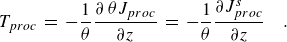 \begin{equation} T_{{proc}} \: = \: - \frac {1}{\theta } \frac {\partial \, \theta J_{{proc}}}{\partial z} \: = \: - \frac {1}{\theta } \frac {\partial J_{{proc}}^s}{\partial z} \quad . \end{equation}
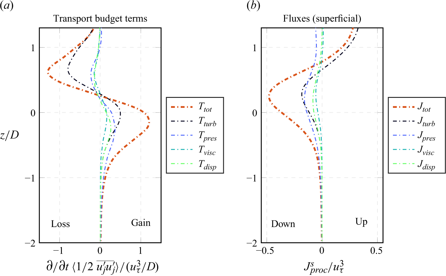
Figure 13. Individual transport terms in the TKE budget and the corresponding superficially averaged TKE fluxes. Case M-300 serves as an example. The shear velocity $u_\tau$
and the sphere diameter
$u_\tau$
and the sphere diameter $D$
are used for normalisation. The vertical coordinate
$D$
are used for normalisation. The vertical coordinate $z$
refers to the geometrically defined interface and is normalised by
$z$
refers to the geometrically defined interface and is normalised by $D$
.
$D$
.
For case M-300, TKE is transported upwards above $z/D \approx 0.7$
and downwards below this position, as indicated by a positive flux above and a negative flux below this point. A similar TKE flux upwards into the free-flow region was documented by Raupach et al. (Reference Raupach, Antonia and Rajagopalan1991) and Mignot et al. (Reference Mignot, Barthelemy and Hurther2009). In the direct proximity of the interface, viscous and dispersive transport cause downward-oriented TKE fluxes of small amplitude. The downward orientation of the dispersive flux contrasts the observations of Shen et al. (Reference Shen, Yuan and Phanikumar2020), who report upward dispersive transport. The turbulent transport
$z/D \approx 0.7$
and downwards below this position, as indicated by a positive flux above and a negative flux below this point. A similar TKE flux upwards into the free-flow region was documented by Raupach et al. (Reference Raupach, Antonia and Rajagopalan1991) and Mignot et al. (Reference Mignot, Barthelemy and Hurther2009). In the direct proximity of the interface, viscous and dispersive transport cause downward-oriented TKE fluxes of small amplitude. The downward orientation of the dispersive flux contrasts the observations of Shen et al. (Reference Shen, Yuan and Phanikumar2020), who report upward dispersive transport. The turbulent transport $T_{turb}$
has a dominant contribution to the removal of TKE from the region near the sphere crests, where the production maximum is found. A large share of the TKE is transported upwards into the free-flow region. Below
$T_{turb}$
has a dominant contribution to the removal of TKE from the region near the sphere crests, where the production maximum is found. A large share of the TKE is transported upwards into the free-flow region. Below $z/D \approx 0.7$
, a negative turbulent flux transports TKE deeper into the sediment bed.
$z/D \approx 0.7$
, a negative turbulent flux transports TKE deeper into the sediment bed.
In contrast to the other TKE transport processes, pressure transport can only cause net vertical transport of $\langle \overline {w^\prime w^\prime } \rangle$
. Even above the crests of the topmost spheres at
$\langle \overline {w^\prime w^\prime } \rangle$
. Even above the crests of the topmost spheres at $z/D \gt 1$
, the corresponding flux has a negative sign, which implies that pressure transport transfers TKE from the free flow region towards and into the sediment bed. At
$z/D \gt 1$
, the corresponding flux has a negative sign, which implies that pressure transport transfers TKE from the free flow region towards and into the sediment bed. At $z/D \approx 0.6$
, further TKE is picked up, such that the downwards-oriented flux reaches its maximum amplitude at approximately
$z/D \approx 0.6$
, further TKE is picked up, such that the downwards-oriented flux reaches its maximum amplitude at approximately $z/D = 0.2$
. Deeper below the interface at
$z/D = 0.2$
. Deeper below the interface at $z/D \lt -0.5$
, pressure transport introduces more TKE than other transport processes. The efficient propagation of vertical velocity fluctuation into deeper sediment layers is likely explained by a superposition of both small-scale pressure fluctuations originating from the interface region and large-scale pressure fluctuations from the free flow region. Under normalisation with the cube of the friction velocity, figure 14 shows the maximal amplitudes of the downward-oriented TKE flux due to pressure transport. Among cases with similar
$z/D \lt -0.5$
, pressure transport introduces more TKE than other transport processes. The efficient propagation of vertical velocity fluctuation into deeper sediment layers is likely explained by a superposition of both small-scale pressure fluctuations originating from the interface region and large-scale pressure fluctuations from the free flow region. Under normalisation with the cube of the friction velocity, figure 14 shows the maximal amplitudes of the downward-oriented TKE flux due to pressure transport. Among cases with similar $Re_K$
, the cases with the largest ratio
$Re_K$
, the cases with the largest ratio $h/D$
exhibit the largest value of
$h/D$
exhibit the largest value of $\max ( | J_{{pres}}^s | ) \, / \, u_\tau ^3$
. In the fully rough regime, the smaller relative roughness for cases with large
$\max ( | J_{{pres}}^s | ) \, / \, u_\tau ^3$
. In the fully rough regime, the smaller relative roughness for cases with large $h/D$
results in a larger bulk velocity
$h/D$
results in a larger bulk velocity $u_b$
, which seems to increase the TKE flux. Also under normalisation with
$u_b$
, which seems to increase the TKE flux. Also under normalisation with $u_b^3$
(not shown here), the flux maxima do not collapse, which supports the idea that effects of free-flow and near-interface scales are superposed. Except for case S-150, the vertical position of the largest downward-oriented TKE flux, which corresponds to the zero-crossing of the budget term, coincides approximately with the drag-based interface position
$u_b^3$
(not shown here), the flux maxima do not collapse, which supports the idea that effects of free-flow and near-interface scales are superposed. Except for case S-150, the vertical position of the largest downward-oriented TKE flux, which corresponds to the zero-crossing of the budget term, coincides approximately with the drag-based interface position $\mu _z$
.
$\mu _z$
.
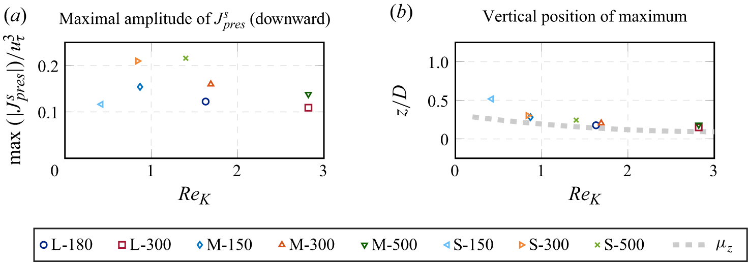
Figure 14. Amplitude of the downward-oriented TKE flux due to pressure transport over the permeability Reynolds number $Re_K$
. (a) Maximal amplitude of the TKE flux due to pressure transport, normalised by the friction velocity
$Re_K$
. (a) Maximal amplitude of the TKE flux due to pressure transport, normalised by the friction velocity $u_\tau ^3$
. (b) Vertical position of the maximum with respect to the geometrically defined interface, whereas
$u_\tau ^3$
. (b) Vertical position of the maximum with respect to the geometrically defined interface, whereas $z$
is normalised by
$z$
is normalised by $D$
. The grey dashed line represents the position
$D$
. The grey dashed line represents the position $\mu _z$
of the drag-based interface.
$\mu _z$
of the drag-based interface.
4.7. Overview of the near-interface WKE budget
In the following, we focus on the WKE budget, which gives us detailed insight into the production, transport and destruction of spatial variance in the time-averaged velocity field. Again, we use case M-300 as an exemplary case for the detailed analysis.
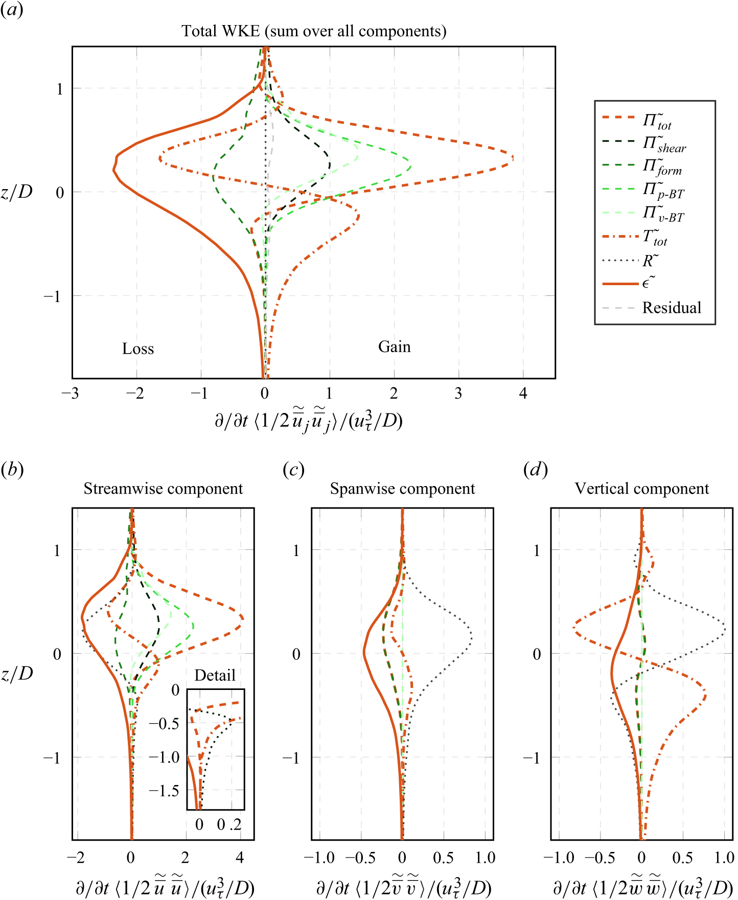
Figure 15. Budgets for the complete WKE and for the individual dispersive normal stresses in the near-interface region. Case M-300 serves as an example. For normalisation, the shear velocity $u_\tau$
and the sphere diameter
$u_\tau$
and the sphere diameter $D$
are used. The vertical coordinate
$D$
are used. The vertical coordinate $z$
refers to the geometrically defined interface and is normalised by
$z$
refers to the geometrically defined interface and is normalised by $D$
. Note that the horizontal axes cover different value ranges.
$D$
. Note that the horizontal axes cover different value ranges.
Figure 15(a) shows the budget of the total WKE. The total production $\Pi _{\textit{tot}}^\sim$
peaks at
$\Pi _{\textit{tot}}^\sim$
peaks at $z/D \approx 0.3$
. From this production maximum, WKE is transported in both directions. Small amounts of WKE are moved in the positive
$z/D \approx 0.3$
. From this production maximum, WKE is transported in both directions. Small amounts of WKE are moved in the positive $z$
-direction, such that the total transport
$z$
-direction, such that the total transport $T_{\textit{tot}}^\sim$
has a positive contribution at
$T_{\textit{tot}}^\sim$
has a positive contribution at $z/D \approx 1$
. The majority of the WKE, however, is relocated into deeper regions of the sediment bed, where the transport constitutes the only positive budget term. Similar to the TKE budget, the maximal dissipation of WKE also takes place slightly below the peak of the WKE production. The total production
$z/D \approx 1$
. The majority of the WKE, however, is relocated into deeper regions of the sediment bed, where the transport constitutes the only positive budget term. Similar to the TKE budget, the maximal dissipation of WKE also takes place slightly below the peak of the WKE production. The total production $\Pi _{\textit{tot}}^\sim$
summarises the shear production
$\Pi _{\textit{tot}}^\sim$
summarises the shear production $\Pi _{shear}^\sim$
, the form-induced production
$\Pi _{shear}^\sim$
, the form-induced production $\Pi _{\textit{form}}^\sim = -\Pi _{\textit{form}}$
and the WKE production that results from interaction with the sphere surfaces via the pressure (
$\Pi _{\textit{form}}^\sim = -\Pi _{\textit{form}}$
and the WKE production that results from interaction with the sphere surfaces via the pressure ( $\Pi _{p\textit{-BT}}^\sim$
) and via viscous stresses (
$\Pi _{p\textit{-BT}}^\sim$
) and via viscous stresses ( $\Pi _{\nu \textit{-BT}}^\sim$
). The form-induced production transfers kinetic energy from the WKE to the TKE and, therefore, appears with a negative sign in the WKE budget. In comparison to the shear production, a larger share of WKE production results from the interactions of the flow field with the solid surfaces of the sediment bed. Notice that the production due to viscous interactions with the sphere surfaces is not considerably smaller than the production due to pressure-based surface interactions.
$\Pi _{\nu \textit{-BT}}^\sim$
). The form-induced production transfers kinetic energy from the WKE to the TKE and, therefore, appears with a negative sign in the WKE budget. In comparison to the shear production, a larger share of WKE production results from the interactions of the flow field with the solid surfaces of the sediment bed. Notice that the production due to viscous interactions with the sphere surfaces is not considerably smaller than the production due to pressure-based surface interactions.
To complete the picture, figure 15(b–d) shows the budgets for the individual WKE components. All four production mechanisms are involved in the budget of $\langle \widetilde {\overline {u}} \, \widetilde {\overline {u}} \rangle$
. Approximately half of the produced variations in the streamwise velocity field are dissipated in the region near the production peak at
$\langle \widetilde {\overline {u}} \, \widetilde {\overline {u}} \rangle$
. Approximately half of the produced variations in the streamwise velocity field are dissipated in the region near the production peak at $z/D \approx 0.3$
. A considerable part of the excessively produced WKE is transferred to
$z/D \approx 0.3$
. A considerable part of the excessively produced WKE is transferred to $\langle \widetilde {\overline {v}} \, \widetilde {\overline {v}} \rangle$
and
$\langle \widetilde {\overline {v}} \, \widetilde {\overline {v}} \rangle$
and $\langle \widetilde {\overline {w}} \, \widetilde {\overline {w}} \rangle$
. The redistributed WKE constitutes the only term with a major positive contribution in the budget of
$\langle \widetilde {\overline {w}} \, \widetilde {\overline {w}} \rangle$
. The redistributed WKE constitutes the only term with a major positive contribution in the budget of $\langle \widetilde {\overline {v}} \, \widetilde {\overline {v}} \rangle$
. The negative sign of the form production term indicates that spatial variations in the lateral velocity field are reduced, while temporal fluctuations
$\langle \widetilde {\overline {v}} \, \widetilde {\overline {v}} \rangle$
. The negative sign of the form production term indicates that spatial variations in the lateral velocity field are reduced, while temporal fluctuations $\langle \overline {v^\prime v^\prime } \rangle$
are generated. Transport processes play a critical role in the budget of
$\langle \overline {v^\prime v^\prime } \rangle$
are generated. Transport processes play a critical role in the budget of $\langle \widetilde {\overline {w}} \, \widetilde {\overline {w}} \rangle$
. Above the interface at
$\langle \widetilde {\overline {w}} \, \widetilde {\overline {w}} \rangle$
. Above the interface at $z/D \approx 0.25$
, inter-component redistribution increases variations in the bed-normal velocity field, whereas only a small amount of these variations is dissipated. While only a small amount is transported upwards, most of the excessively introduced
$z/D \approx 0.25$
, inter-component redistribution increases variations in the bed-normal velocity field, whereas only a small amount of these variations is dissipated. While only a small amount is transported upwards, most of the excessively introduced $\langle \widetilde {\overline {w}} \, \widetilde {\overline {w}} \rangle$
is transported downwards into the sediment bed. In those deeper regions, the redistribution mechanism
$\langle \widetilde {\overline {w}} \, \widetilde {\overline {w}} \rangle$
is transported downwards into the sediment bed. In those deeper regions, the redistribution mechanism $R^\sim$
acts in the opposite direction, as it takes WKE out of
$R^\sim$
acts in the opposite direction, as it takes WKE out of $\langle \widetilde {\overline {w}} \, \widetilde {\overline {w}} \rangle$
and introduces it even back into
$\langle \widetilde {\overline {w}} \, \widetilde {\overline {w}} \rangle$
and introduces it even back into $\langle \widetilde {\overline {u}} \, \widetilde {\overline {u}} \rangle$
, as shown by the detail in figure 15(b).
$\langle \widetilde {\overline {u}} \, \widetilde {\overline {u}} \rangle$
, as shown by the detail in figure 15(b).
4.8. Scaling of WKE sources and sinks
Figure 15 has shown that shear production by dispersive stresses $\Pi _{shear}^\sim$
, as well as
$\Pi _{shear}^\sim$
, as well as $\Pi _{p\textit{-BT}}^\sim$
and
$\Pi _{p\textit{-BT}}^\sim$
and $\Pi _{\nu \textit{-BT}}^\sim$
produce WKE in the interface region. Besides the dissipation, the form-induced production of TKE acts as a sink of WKE. Figure 16(a) shows the maximal values of different WKE sources and sinks, which are plotted over
$\Pi _{\nu \textit{-BT}}^\sim$
produce WKE in the interface region. Besides the dissipation, the form-induced production of TKE acts as a sink of WKE. Figure 16(a) shows the maximal values of different WKE sources and sinks, which are plotted over $Re_K$
. The values are normalised by the friction velocity
$Re_K$
. The values are normalised by the friction velocity $u_\tau$
and the sphere diameter
$u_\tau$
and the sphere diameter $D$
. Figure 16(b) provides the elevations at which the maxima are found.
$D$
. Figure 16(b) provides the elevations at which the maxima are found.
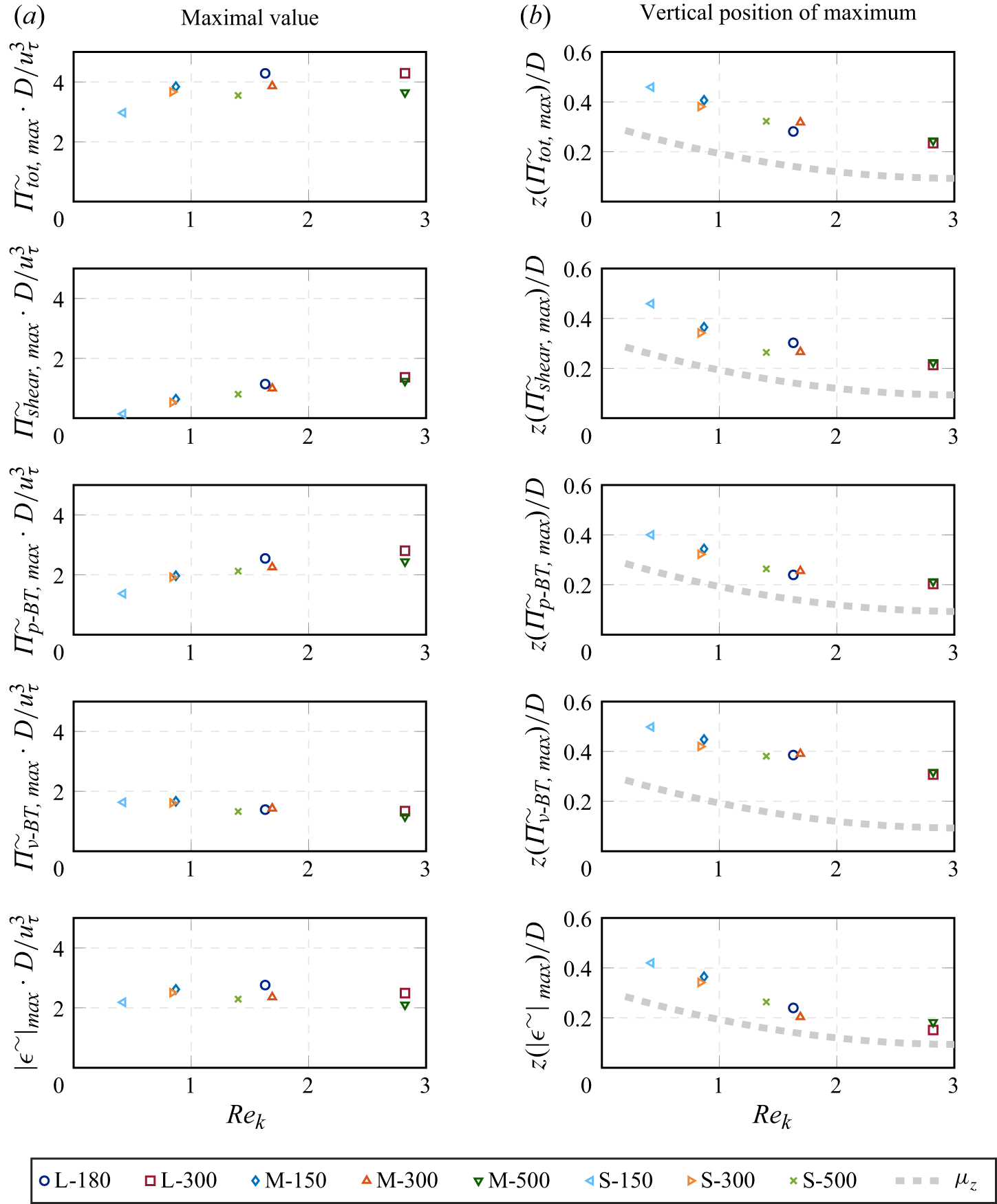
Figure 16. Scaling of production mechanisms and dissipation of WKE with $Re_K$
. (a) Maximal values of the processes normalised with the friction velocity
$Re_K$
. (a) Maximal values of the processes normalised with the friction velocity $u_\tau$
and the sphere diameter
$u_\tau$
and the sphere diameter $D$
. (b) Position of the maxima with respect to the geometrically defined interface, whereas the vertical coordinate
$D$
. (b) Position of the maxima with respect to the geometrically defined interface, whereas the vertical coordinate $z$
is normalised by
$z$
is normalised by $D$
. The grey dashed line represents the position
$D$
. The grey dashed line represents the position $\mu _z$
of the drag-based interface. The total production
$\mu _z$
of the drag-based interface. The total production $\Pi _{\textit{tot}}^\sim$
summarises the processes
$\Pi _{\textit{tot}}^\sim$
summarises the processes $\Pi _{shear}^\sim$
,
$\Pi _{shear}^\sim$
, $\Pi _{\text{$p$-}BT}^\sim$
and
$\Pi _{\text{$p$-}BT}^\sim$
and $\Pi _{\text{$\nu $-}BT}^\sim$
, whereas
$\Pi _{\text{$\nu $-}BT}^\sim$
, whereas $\epsilon ^\sim$
is the dissipation.
$\epsilon ^\sim$
is the dissipation.
For $Re_K \leq 1$
, the maximum of the total production becomes larger with increasing
$Re_K \leq 1$
, the maximum of the total production becomes larger with increasing $Re_K$
, whereas its value seems to saturate in the region of
$Re_K$
, whereas its value seems to saturate in the region of $Re_K \gt 1$
. With increasing
$Re_K \gt 1$
. With increasing $Re_K$
, the maximum value of WKE shear production increases monotonically. For the transitionally rough case S-150, dispersive shear stresses are very small, such that hardly any shear production is observed. The shear production maximum is found at progressively lower heights with increasing
$Re_K$
, the maximum value of WKE shear production increases monotonically. For the transitionally rough case S-150, dispersive shear stresses are very small, such that hardly any shear production is observed. The shear production maximum is found at progressively lower heights with increasing $Re_K$
. For all simulated cases,
$Re_K$
. For all simulated cases, $\Pi _{p\textit{-BT}}^\sim$
, i.e. the WKE production due to work of the double-averaged flow field against the pressure drag, exceeds the shear production, while it also increases monotonously with increasing
$\Pi _{p\textit{-BT}}^\sim$
, i.e. the WKE production due to work of the double-averaged flow field against the pressure drag, exceeds the shear production, while it also increases monotonously with increasing $Re_K$
. The maximum of
$Re_K$
. The maximum of $\Pi _{p\textit{-BT}}^\sim$
is found at approximately the same vertical position as the maximal shear production. The production
$\Pi _{p\textit{-BT}}^\sim$
is found at approximately the same vertical position as the maximal shear production. The production $\Pi _{\nu \textit{-BT}}^\sim$
, which results from the work of the double-averaged flow field against the viscous drag from in-plane velocity variations, decreases slightly with increasing
$\Pi _{\nu \textit{-BT}}^\sim$
, which results from the work of the double-averaged flow field against the viscous drag from in-plane velocity variations, decreases slightly with increasing $Re_K$
. For the transitionally rough case S-150, the maximum of
$Re_K$
. For the transitionally rough case S-150, the maximum of $\Pi _{\nu \textit{-BT}}^\sim$
is higher than the maximum of
$\Pi _{\nu \textit{-BT}}^\sim$
is higher than the maximum of $\Pi _{p\textit{-BT}}^\sim$
, indicating an important role of viscous effects. With increasing
$\Pi _{p\textit{-BT}}^\sim$
, indicating an important role of viscous effects. With increasing $Re_K$
, the relative importance of
$Re_K$
, the relative importance of $\Pi _{\nu \textit{-BT}}^\sim$
in comparison to other WKE production mechanisms declines but remains noticeable. The maximum of
$\Pi _{\nu \textit{-BT}}^\sim$
in comparison to other WKE production mechanisms declines but remains noticeable. The maximum of $\Pi _{\nu \textit{-BT}}^\sim$
is found near the crests of the topmost spheres and thus at a greater elevation than the maxima of other processes. For all cases, the maximum value of the dissipation is smaller than that of the total production of WKE, while figure 15 indicates that dissipation takes place over a wider region. With increasing
$\Pi _{\nu \textit{-BT}}^\sim$
is found near the crests of the topmost spheres and thus at a greater elevation than the maxima of other processes. For all cases, the maximum value of the dissipation is smaller than that of the total production of WKE, while figure 15 indicates that dissipation takes place over a wider region. With increasing $Re_K$
, the form-induced production of TKE (figure 11) also removes progressively larger amounts of WKE. The dissipation maximum is found at approximately the same elevation as the maximum of the total production. As already observed for the TKE, the maxima of the WKE sources and sinks move to lower vertical positions with increasing
$Re_K$
, the form-induced production of TKE (figure 11) also removes progressively larger amounts of WKE. The dissipation maximum is found at approximately the same elevation as the maximum of the total production. As already observed for the TKE, the maxima of the WKE sources and sinks move to lower vertical positions with increasing $Re_K$
. Thus, they follow a trend in the equally
$Re_K$
. Thus, they follow a trend in the equally $Re_K$
-dependent position
$Re_K$
-dependent position $\mu _z$
of the drag-based interface, which is marked by a grey dashed line in figure 16.
$\mu _z$
of the drag-based interface, which is marked by a grey dashed line in figure 16.
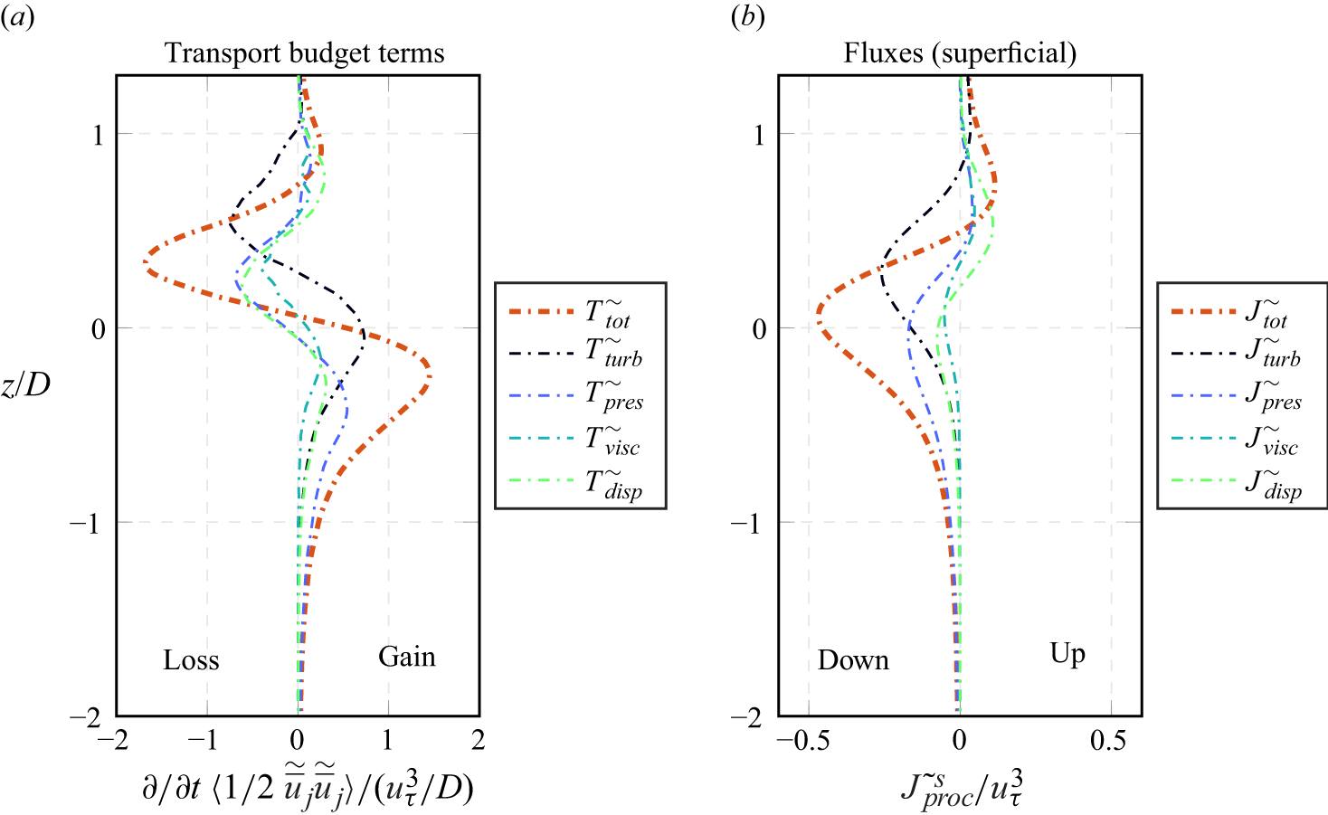
Figure 17. Individual transport terms in the WKE budget and the corresponding superficially averaged WKE fluxes. Case M-300 serves as an example. The shear velocity $u_\tau$
and the sphere diameter
$u_\tau$
and the sphere diameter $D$
are used for normalisation. The vertical coordinate
$D$
are used for normalisation. The vertical coordinate $z$
refers to the geometrically defined interface and is normalised by
$z$
refers to the geometrically defined interface and is normalised by $D$
.
$D$
.
4.9. WKE transport and fluxes
As done for the TKE in § 4.6, we continue with a detailed discussion of the process-specific transport terms $T_{{proc}}^\sim$
in the WKE budget, which are shown in figure 17(a). The corresponding superficially double-averaged WKE fluxes
$T_{{proc}}^\sim$
in the WKE budget, which are shown in figure 17(a). The corresponding superficially double-averaged WKE fluxes $J^{\sim s}_{{proc}}$
are provided in figure 17(b), and the relation between both quantities is given by (4.1). The total transport moves a large part of the WKE from the region near
$J^{\sim s}_{{proc}}$
are provided in figure 17(b), and the relation between both quantities is given by (4.1). The total transport moves a large part of the WKE from the region near $z/D \approx 0.3$
. As shown by the large amplitude of the negative flux around
$z/D \approx 0.3$
. As shown by the large amplitude of the negative flux around $z/D=0$
, WKE is predominantly transported downwards. Only turbulent transport seems to transfer a small amount of spatial velocity variations into the region
$z/D=0$
, WKE is predominantly transported downwards. Only turbulent transport seems to transfer a small amount of spatial velocity variations into the region $z/D \gt 1$
, where the WKE is small, but not absolutely zero. Viscous and dispersive transport cause comparatively smaller fluxes
$z/D \gt 1$
, where the WKE is small, but not absolutely zero. Viscous and dispersive transport cause comparatively smaller fluxes $J^{\sim s}_{visc}$
and
$J^{\sim s}_{visc}$
and $J^{\sim s}_{disp}$
, which relocate WKE only in direct proximity of the interface, whereas they neither affect the free flow region nor greater depths of the sediment bed. Compared with turbulent transport, pressure transport causes a similarly strong downwards oriented WKE flux
$J^{\sim s}_{disp}$
, which relocate WKE only in direct proximity of the interface, whereas they neither affect the free flow region nor greater depths of the sediment bed. Compared with turbulent transport, pressure transport causes a similarly strong downwards oriented WKE flux $J^{\sim s}_{{pres}}$
from the interface region. The flux from pressure transport, however, peaks at a lower position and also introduces spatial velocity variations into greater depths of
$J^{\sim s}_{{pres}}$
from the interface region. The flux from pressure transport, however, peaks at a lower position and also introduces spatial velocity variations into greater depths of $z/D \lt -1$
. In contrast to that, the pressure transport hardly introduces any spatial velocity variations in the free flow region.
$z/D \lt -1$
. In contrast to that, the pressure transport hardly introduces any spatial velocity variations in the free flow region.
Vertical pressure-driven transport propagates WKE into deeper regions of the sediment and acts via spatial variations of $\overline {w}$
, which makes the process also highly relevant for dispersive mass transport in the hyporheic zone. That motivates us to investigate the scaling behaviour of the flux
$\overline {w}$
, which makes the process also highly relevant for dispersive mass transport in the hyporheic zone. That motivates us to investigate the scaling behaviour of the flux $J^{\sim s}_{{pres}}$
in detail. As shown by figure 18, the maximal amplitude of the downward oriented flux is reached slightly below
$J^{\sim s}_{{pres}}$
in detail. As shown by figure 18, the maximal amplitude of the downward oriented flux is reached slightly below $z = \mu _z$
and it follows the drag-based interface. When the maximal amplitude of the downward-oriented flux is normalised by
$z = \mu _z$
and it follows the drag-based interface. When the maximal amplitude of the downward-oriented flux is normalised by $u_\tau ^3$
and plotted over
$u_\tau ^3$
and plotted over $Re_K$
, we observe a nonlinear increase, such that a clearly interpretable scaling behaviour cannot be deduced. To find an appropriate scaling, an idealised scenario of pressure pumping is sketched in Appendix C, and different terms are evaluated analytically. The analytic solutions suggest that
$Re_K$
, we observe a nonlinear increase, such that a clearly interpretable scaling behaviour cannot be deduced. To find an appropriate scaling, an idealised scenario of pressure pumping is sketched in Appendix C, and different terms are evaluated analytically. The analytic solutions suggest that $J^{\sim s}_{{pres}}$
scales with
$J^{\sim s}_{{pres}}$
scales with $({K}/{\nu \rho ^2}) \hat {p}^2 k_x$
, where
$({K}/{\nu \rho ^2}) \hat {p}^2 k_x$
, where $\hat {p}$
represents the amplitude of a regular pressure variation at the interface, while
$\hat {p}$
represents the amplitude of a regular pressure variation at the interface, while $k_x$
is the wavenumber of the regular pressure variation. According to the Kozeny–Carman equation, the permeability
$k_x$
is the wavenumber of the regular pressure variation. According to the Kozeny–Carman equation, the permeability $K$
scales with
$K$
scales with $D^2$
. Further, we assume that
$D^2$
. Further, we assume that $\hat {p}$
is proportional to
$\hat {p}$
is proportional to $\rho u_\tau ^2$
and that
$\rho u_\tau ^2$
and that $k_x$
is proportional to
$k_x$
is proportional to $1/D$
. These assumptions suggest a scaling of
$1/D$
. These assumptions suggest a scaling of $J^{\sim s}_{{pres}}$
with
$J^{\sim s}_{{pres}}$
with $u_\tau ^4 D / \nu$
. Figure 18 shows that, under normalisation with
$u_\tau ^4 D / \nu$
. Figure 18 shows that, under normalisation with $u_\tau ^4 D / \nu$
, the highest value of
$u_\tau ^4 D / \nu$
, the highest value of $J^{\sim s}_{{pres}}$
is reached for cases with
$J^{\sim s}_{{pres}}$
is reached for cases with $Re_K \approx 1$
, whereas it decreases monotonically for higher
$Re_K \approx 1$
, whereas it decreases monotonically for higher $Re_K \gt 1$
. Again, no interpretable scaling behaviour can be observed. Elliott & Brooks (Reference Elliott and Brooks1997) propose a scaling of the pressure variations with the bulk velocity, which similarly does not seem to apply for our cases without macroscopic bed forms (not shown here). In § 5, we discuss a potential scaling of the pressure-driven processes in the near-interface region, which includes the roughness-induced dimensionless velocity shift
$Re_K \gt 1$
. Again, no interpretable scaling behaviour can be observed. Elliott & Brooks (Reference Elliott and Brooks1997) propose a scaling of the pressure variations with the bulk velocity, which similarly does not seem to apply for our cases without macroscopic bed forms (not shown here). In § 5, we discuss a potential scaling of the pressure-driven processes in the near-interface region, which includes the roughness-induced dimensionless velocity shift $\Delta u^+$
as an additional parameter.
$\Delta u^+$
as an additional parameter.
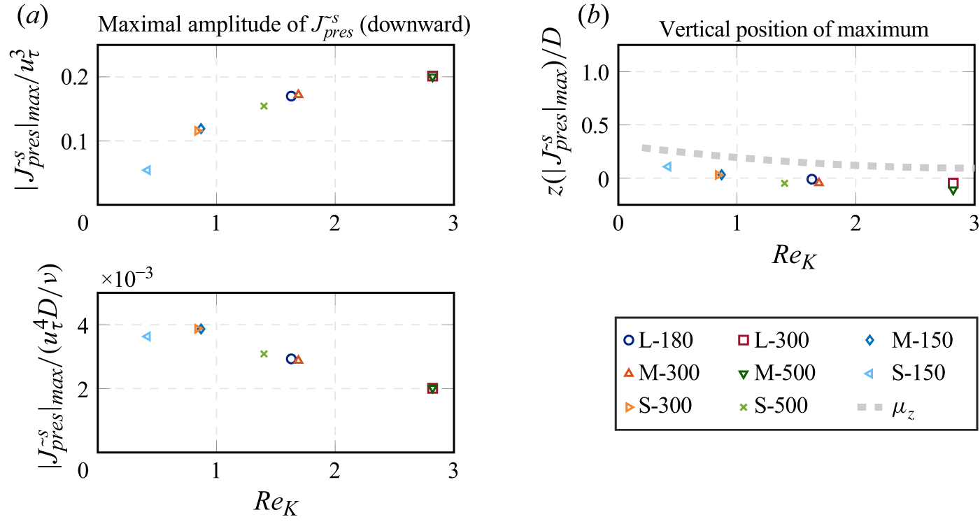
Figure 18. Amplitude of the downward-oriented WKE flux due to pressure transport over the permeability Reynolds number $Re_K$
. (a) Maximal amplitude of the WKE flux due to pressure transport, normalised by the friction velocity
$Re_K$
. (a) Maximal amplitude of the WKE flux due to pressure transport, normalised by the friction velocity $u_\tau ^3$
. (b) Vertical position of the maxima with respect to the geometrically defined interface, whereas
$u_\tau ^3$
. (b) Vertical position of the maxima with respect to the geometrically defined interface, whereas $z$
is normalised by
$z$
is normalised by $D$
. The grey dashed line represents the position
$D$
. The grey dashed line represents the position $\mu _z$
of the drag-based interface.
$\mu _z$
of the drag-based interface.
5. Discussion
Finnigan (Reference Finnigan2000) stated that work against the viscous component of the canopy drag leads to a direct dissipation of MKE into heat. Revisiting the budget equations, however, we encounter a term which represents an energy transfer from MKE to WKE via viscous interaction between the flow and the solid surfaces. While the term results formally from a rigorous application of the rules for spatial derivatives within the horizontal averaging framework (e.g. Giménez-Curto & Lera Reference Giménez-Curto and Lera1996), we can also find a simple example, which intuitively illustrates the existence of such a viscosity-based WKE production mechanism (see figure 1). As the studies of Yuan & Piomelli (Reference Yuan and Piomelli2014) or Ghodke & Apte (Reference Ghodke and Apte2018) do not explicitly mention WKE production via viscous interaction with solid surfaces, the question remains if this process is relevant in the context of turbulent flow over a random sphere pack.
For flow over a random sphere pack at $Re_K \lt 3$
, our results suggest a clear ‘yes’. For the transitionally rough case S-150, viscous- and pressure-based surface interactions contribute to the WKE production in approximately equal parts. In contrast, the shear production of WKE is negligible for case S-150, which can be explained by the strong wall-blocking and the very low dispersive shear stresses near the interface (v.Wenczowski & Manhart Reference v. Wenczowski and Manhart2024). Even for the cases L-300 and M-500 with
$Re_K \lt 3$
, our results suggest a clear ‘yes’. For the transitionally rough case S-150, viscous- and pressure-based surface interactions contribute to the WKE production in approximately equal parts. In contrast, the shear production of WKE is negligible for case S-150, which can be explained by the strong wall-blocking and the very low dispersive shear stresses near the interface (v.Wenczowski & Manhart Reference v. Wenczowski and Manhart2024). Even for the cases L-300 and M-500 with $Re_K \approx 2.8$
, the relative contribution of the WKE production due to viscous surface interaction does not become negligible, though it is smaller than the dominant WKE production due to pressure drag. Accordingly, the shift in the relative impact of the production mechanism reflects the transition of the roughness regime (Raupach et al. Reference Raupach, Antonia and Rajagopalan1991; Jiménez Reference Jiménez2004; Kadivar et al. Reference Kadivar, Tormey and McGranaghan2021) from the transitionally rough to the fully rough regime. An extrapolation of this trend could explain that in atmospheric flow (e.g Raupach & Shaw Reference Raupach and Shaw1982), the WKE production via viscous interaction could be neglected for extreme roughness and permeability, which is not generally justified for hyporheic flow problems.
$Re_K \approx 2.8$
, the relative contribution of the WKE production due to viscous surface interaction does not become negligible, though it is smaller than the dominant WKE production due to pressure drag. Accordingly, the shift in the relative impact of the production mechanism reflects the transition of the roughness regime (Raupach et al. Reference Raupach, Antonia and Rajagopalan1991; Jiménez Reference Jiménez2004; Kadivar et al. Reference Kadivar, Tormey and McGranaghan2021) from the transitionally rough to the fully rough regime. An extrapolation of this trend could explain that in atmospheric flow (e.g Raupach & Shaw Reference Raupach and Shaw1982), the WKE production via viscous interaction could be neglected for extreme roughness and permeability, which is not generally justified for hyporheic flow problems.
With increasing $Re_K$
, the form-induced production converts progressively larger amounts of WKE into TKE. Even for the fully rough cases in this study, however, the form production remains small in comparison to the shear production of TKE, which appears to be the dominant process in the near-interface TKE budget. This observation agrees with the findings of Fang et al. (Reference Fang, Han, He and Dey2018) and Shen et al. (Reference Shen, Yuan and Phanikumar2020). The investigation of an instantaneous field showed that form-induced production takes place within a thin layer near the sediment bed surface and occurs on small scales, which are comparable to the sphere diameter. As stated by Finnigan (Reference Finnigan2000), the introduction of TKE on smaller length scales explains why wake production is less efficient than shear production.
$Re_K$
, the form-induced production converts progressively larger amounts of WKE into TKE. Even for the fully rough cases in this study, however, the form production remains small in comparison to the shear production of TKE, which appears to be the dominant process in the near-interface TKE budget. This observation agrees with the findings of Fang et al. (Reference Fang, Han, He and Dey2018) and Shen et al. (Reference Shen, Yuan and Phanikumar2020). The investigation of an instantaneous field showed that form-induced production takes place within a thin layer near the sediment bed surface and occurs on small scales, which are comparable to the sphere diameter. As stated by Finnigan (Reference Finnigan2000), the introduction of TKE on smaller length scales explains why wake production is less efficient than shear production.
In the present study, we used the inflection point of the porosity profile as a geometrical interface definition and the sphere diameter $D$
as an interface length scale. Within this reference frame, the maxima of production and dissipation terms are found at progressively lower positions with increasing
$D$
as an interface length scale. Within this reference frame, the maxima of production and dissipation terms are found at progressively lower positions with increasing $Re_K$
. In v.Wenczowski & Manhart (Reference v. Wenczowski and Manhart2024), we proposed a drag-based interface description, where the height
$Re_K$
. In v.Wenczowski & Manhart (Reference v. Wenczowski and Manhart2024), we proposed a drag-based interface description, where the height $\mu _z$
represents the position of maximal momentum absorption near the interface and
$\mu _z$
represents the position of maximal momentum absorption near the interface and $\sigma _z$
quantifies the spread of the region in which the momentum is absorbed. We used
$\sigma _z$
quantifies the spread of the region in which the momentum is absorbed. We used $\mu _z$
to define the interface position and a consistent friction velocity was computed as
$\mu _z$
to define the interface position and a consistent friction velocity was computed as $u_\tau ^\mu = \sqrt {g_x (h-\mu _z)}$
. Together with
$u_\tau ^\mu = \sqrt {g_x (h-\mu _z)}$
. Together with $\sigma _z$
, an interface coordinate was defined as
$\sigma _z$
, an interface coordinate was defined as $\gamma = (z-\mu _z) / \sigma _z$
. In the following, we deviate from the geometric interface definition and discuss the scaling behaviour of the shear production in the drag-based framework.
$\gamma = (z-\mu _z) / \sigma _z$
. In the following, we deviate from the geometric interface definition and discuss the scaling behaviour of the shear production in the drag-based framework.
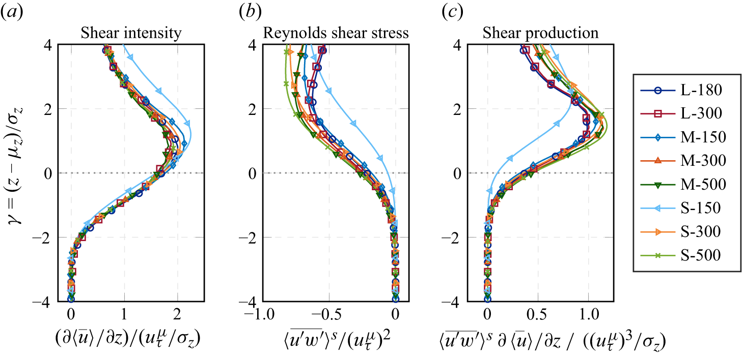
Figure 19. Near-interface profiles of the shear intensity, the Reynolds shear stress and the resulting shear production of TKE. The vertical coordinate $\gamma$
considers the drag-based interface position at
$\gamma$
considers the drag-based interface position at $z=\mu _z$
and uses the spread
$z=\mu _z$
and uses the spread $\sigma _z$
of the drag distribution as a length scale. The friction velocity
$\sigma _z$
of the drag distribution as a length scale. The friction velocity $u_\tau ^\mu$
is consistent with the drag-based interface at
$u_\tau ^\mu$
is consistent with the drag-based interface at $z=\mu _z$
.
$z=\mu _z$
.
Figure 19 shows that $\partial \langle \overline {u} \rangle / \partial z$
scales with
$\partial \langle \overline {u} \rangle / \partial z$
scales with $u_\tau ^\mu / \sigma _z$
, which means that a momentum absorption over a wider region reduces the shear intensity. Further, the figure shows that Reynolds shear stress
$u_\tau ^\mu / \sigma _z$
, which means that a momentum absorption over a wider region reduces the shear intensity. Further, the figure shows that Reynolds shear stress $\langle \overline {u^\prime w^\prime } \rangle ^s$
scales approximately, though not perfectly, with
$\langle \overline {u^\prime w^\prime } \rangle ^s$
scales approximately, though not perfectly, with $(u_\tau ^\mu )^2$
. Together, both observations explain the scaling behaviour of the shear production term with
$(u_\tau ^\mu )^2$
. Together, both observations explain the scaling behaviour of the shear production term with $( u_\tau ^\mu )^3 / \sigma _z$
, i.e. with quantities that are characteristic for the interface region. Only the shear production profile of the transitionally rough case S-150 deviates strongly from the profiles of the remaining hydraulically rough cases, which collapse reasonably well when plotted against
$( u_\tau ^\mu )^3 / \sigma _z$
, i.e. with quantities that are characteristic for the interface region. Only the shear production profile of the transitionally rough case S-150 deviates strongly from the profiles of the remaining hydraulically rough cases, which collapse reasonably well when plotted against $\gamma$
. In combination with the observed trend that the maximum values of other processes of the TKE budget similarly follow the drag-based interface position (figure 11), the similarity of the shear production distribution further underlines the flow-dynamical relevance of this interface definition.
$\gamma$
. In combination with the observed trend that the maximum values of other processes of the TKE budget similarly follow the drag-based interface position (figure 11), the similarity of the shear production distribution further underlines the flow-dynamical relevance of this interface definition.
The similarity of the profiles suggests that the TKE shear production scales with interface-related length and velocity scales. In outer scaling with $u_\tau$
and
$u_\tau$
and $h$
, this observation explains why the near-interface TKE production peak flattens out with progressively larger
$h$
, this observation explains why the near-interface TKE production peak flattens out with progressively larger $Re_K$
. Far from the interface, however, the TKE budget terms of cases with similar
$Re_K$
. Far from the interface, however, the TKE budget terms of cases with similar $Re_\tau$
show a good similarity in outer scaling (see figure 9). This co-existence of two differently scaling regions indicates that these regions hardly influence each other. The notion of a certain, yet by far not complete, separation between a near-interface region and an outer layer is supported by the observation of a layer at
$Re_\tau$
show a good similarity in outer scaling (see figure 9). This co-existence of two differently scaling regions indicates that these regions hardly influence each other. The notion of a certain, yet by far not complete, separation between a near-interface region and an outer layer is supported by the observation of a layer at $z/h \approx 0.4$
, where dissipation and production budget terms are in equilibrium, whereas transport terms hardly play a role.
$z/h \approx 0.4$
, where dissipation and production budget terms are in equilibrium, whereas transport terms hardly play a role.
Within the horizontal double-averaging framework, the pressure diffusion in bed-normal direction only acts via the vertical velocity component $w$
. In contrast to other transport processes, pressure-based vertical transport propagates temporal fluctuations or spatial variations of the velocity field into deeper regions of the sediment bed. The interface also seems to be a source region of TKE, which is transported downwards by pressure diffusion. However, we also observe downward-oriented pressure-based transport of temporal velocity fluctuation from the free-flow region. The interface and free-flow region are therefore not entirely decoupled. In contrast to that, pressure diffusion of WKE only acts between the interface region and the sediment bed below. The exclusive dependency on
$w$
. In contrast to other transport processes, pressure-based vertical transport propagates temporal fluctuations or spatial variations of the velocity field into deeper regions of the sediment bed. The interface also seems to be a source region of TKE, which is transported downwards by pressure diffusion. However, we also observe downward-oriented pressure-based transport of temporal velocity fluctuation from the free-flow region. The interface and free-flow region are therefore not entirely decoupled. In contrast to that, pressure diffusion of WKE only acts between the interface region and the sediment bed below. The exclusive dependency on $Re_K$
is a further indication that the free-flow region is not involved. To discuss the WKE budget terms further, we draw parallels to a simplified two-dimensional scenario, which is sketched in Appendix C. On the surface of a permeable bed, a regular pressure variation characterised by a single wavenumber
$Re_K$
is a further indication that the free-flow region is not involved. To discuss the WKE budget terms further, we draw parallels to a simplified two-dimensional scenario, which is sketched in Appendix C. On the surface of a permeable bed, a regular pressure variation characterised by a single wavenumber $k_x$
is prescribed as a boundary condition and drives the flow field in the porous medium. For this simplified scenario, terms representing pressure-driven mechanisms can be evaluated analytically. The analytic solution predicts that the amplitude of the downward oriented flux of
$k_x$
is prescribed as a boundary condition and drives the flow field in the porous medium. For this simplified scenario, terms representing pressure-driven mechanisms can be evaluated analytically. The analytic solution predicts that the amplitude of the downward oriented flux of $\langle \widetilde {\overline {w}} \, \widetilde {\overline {w}} \rangle$
is largest at the surface of the permeable bed, where the driving pressure field is applied as a boundary condition. In agreement with that, our simulations show that the maximal amplitude of the flux
$\langle \widetilde {\overline {w}} \, \widetilde {\overline {w}} \rangle$
is largest at the surface of the permeable bed, where the driving pressure field is applied as a boundary condition. In agreement with that, our simulations show that the maximal amplitude of the flux $J_{{pres}}^{\sim s} = \theta \langle \widetilde {\overline {p}} \widetilde {\overline {w}} \rangle$
is found only slightly below the drag-based interface at
$J_{{pres}}^{\sim s} = \theta \langle \widetilde {\overline {p}} \widetilde {\overline {w}} \rangle$
is found only slightly below the drag-based interface at $z=\mu _z$
. Also, the analytical solution agrees with the observation that the pressure-diffusion mechanism acts as a source for vertical velocity variations in deeper regions of the sediment bed (figure 17). Beyond that, a pressure redistribution from the vertical velocity variation to the bed-parallel velocity variation is predicted by the analytical solution, which we also see in the simulations at greater depths (figure 15). These points indicate that the behaviour of the budget terms in deeper regions represents a pressure pumping scenario, which agrees with the observation of Shen et al. (Reference Shen, Yuan and Phanikumar2022) for irregular rough surfaces. In the near-interface region, this pumping scenario is superposed by other processes, which are not captured by the simplified scenario with an unresolved interface region. Among those processes is the near-interface pressure redistribution from
$z=\mu _z$
. Also, the analytical solution agrees with the observation that the pressure-diffusion mechanism acts as a source for vertical velocity variations in deeper regions of the sediment bed (figure 17). Beyond that, a pressure redistribution from the vertical velocity variation to the bed-parallel velocity variation is predicted by the analytical solution, which we also see in the simulations at greater depths (figure 15). These points indicate that the behaviour of the budget terms in deeper regions represents a pressure pumping scenario, which agrees with the observation of Shen et al. (Reference Shen, Yuan and Phanikumar2022) for irregular rough surfaces. In the near-interface region, this pumping scenario is superposed by other processes, which are not captured by the simplified scenario with an unresolved interface region. Among those processes is the near-interface pressure redistribution from $\langle \widetilde {\overline {u}} \, \widetilde {\overline {u}} \rangle$
towards
$\langle \widetilde {\overline {u}} \, \widetilde {\overline {u}} \rangle$
towards $\langle \widetilde {\overline {v}} \, \widetilde {\overline {v}} \rangle$
and
$\langle \widetilde {\overline {v}} \, \widetilde {\overline {v}} \rangle$
and $\langle \widetilde {\overline {w}} \, \widetilde {\overline {w}} \rangle$
. This finding emphasises the role of the topmost sediment layer, which was highlighted by Karra et al. (Reference Karra, Apte, He and Scheibe2023).
$\langle \widetilde {\overline {w}} \, \widetilde {\overline {w}} \rangle$
. This finding emphasises the role of the topmost sediment layer, which was highlighted by Karra et al. (Reference Karra, Apte, He and Scheibe2023).
The amount of WKE, which is transferred into $\langle \widetilde {\overline {w}} \, \widetilde {\overline {w}} \rangle$
and transported downwards, is neither proportional to
$\langle \widetilde {\overline {w}} \, \widetilde {\overline {w}} \rangle$
and transported downwards, is neither proportional to $u_\tau ^3$
nor to
$u_\tau ^3$
nor to $u_\tau ^4$
(figure 18), such that we assume that it is necessary to include information about the roughness into a potential scaling relation. In figure 20, the profiles of pressure redistribution and pressure transport terms are plotted against the drag-based interface coordinate
$u_\tau ^4$
(figure 18), such that we assume that it is necessary to include information about the roughness into a potential scaling relation. In figure 20, the profiles of pressure redistribution and pressure transport terms are plotted against the drag-based interface coordinate $\gamma$
. For the normalisation, we use
$\gamma$
. For the normalisation, we use ${(u_\tau ^\mu )^3 \Delta u^+}/{\sigma _z}$
, where
${(u_\tau ^\mu )^3 \Delta u^+}/{\sigma _z}$
, where $u_\tau ^\mu$
represents the interface-adapted friction velocity and
$u_\tau ^\mu$
represents the interface-adapted friction velocity and $\sigma _z$
acts as an interfacial length scale. The dimensionless parameter
$\sigma _z$
acts as an interfacial length scale. The dimensionless parameter $\Delta u^+$
represents the shift of the dimensionless velocity profile with respect to the smooth-wall flow case at comparable
$\Delta u^+$
represents the shift of the dimensionless velocity profile with respect to the smooth-wall flow case at comparable $Re_\tau$
(figure 5). Accordingly, the value of
$Re_\tau$
(figure 5). Accordingly, the value of $\Delta u^+$
can be seen as a robust proxy for the cumulative impact of the roughness. The similarities among the normalised profiles indicate that the amount of WKE that is transferred into
$\Delta u^+$
can be seen as a robust proxy for the cumulative impact of the roughness. The similarities among the normalised profiles indicate that the amount of WKE that is transferred into $\langle \widetilde {\overline {w}} \, \widetilde {\overline {w}} \rangle$
and transported into deeper regions scales well with
$\langle \widetilde {\overline {w}} \, \widetilde {\overline {w}} \rangle$
and transported into deeper regions scales well with ${(u_\tau ^\mu )^3 \Delta u^+}/{\sigma _z}$
in both the transitionally rough and the fully rough regime. As shown in figure 5,
${(u_\tau ^\mu )^3 \Delta u^+}/{\sigma _z}$
in both the transitionally rough and the fully rough regime. As shown in figure 5, $\Delta u^+$
increases monotonically, but nonlinearly, with
$\Delta u^+$
increases monotonically, but nonlinearly, with $Re_K$
.
$Re_K$
.
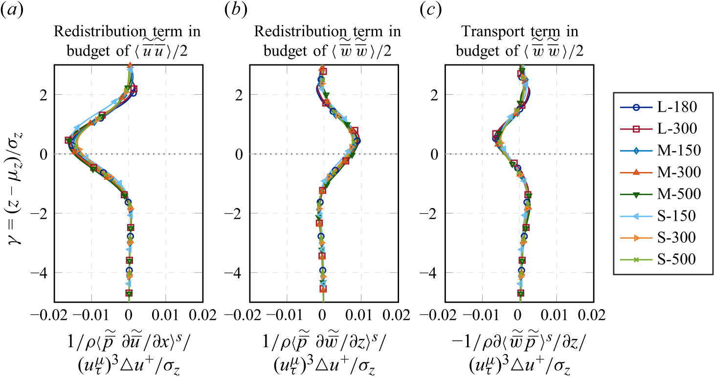
Figure 20. (a,b) Near-interface profiles of WKE redistribution terms and (c) of the pressure transport term. The vertical coordinate $\gamma$
considers the drag-based interface position at
$\gamma$
considers the drag-based interface position at $z=\mu _z$
and uses the spread
$z=\mu _z$
and uses the spread $\sigma _z$
of the drag distribution as a length scale. The friction velocity
$\sigma _z$
of the drag distribution as a length scale. The friction velocity $u_\tau ^\mu$
is consistent with the drag-based interface at
$u_\tau ^\mu$
is consistent with the drag-based interface at $z=\mu _z$
. The dimensionless velocity shift
$z=\mu _z$
. The dimensionless velocity shift $\Delta u^+$
includes the effect of roughness.
$\Delta u^+$
includes the effect of roughness.
6. Conclusions
Based on previously validated data from pore-resolved direct numerical simulations, we evaluated the double-averaged budgets of both turbulent kinetic energy (TKE) and wake kinetic energy (WKE) for turbulent flows over mono-disperse random sphere packs. Eight cases were analysed and act as sampling points within a parameter space, which is spanned by friction Reynolds numbers $Re_\tau \in [150, 500]$
and permeability Reynolds numbers
$Re_\tau \in [150, 500]$
and permeability Reynolds numbers $Re_K \in [0.4, 2.8]$
. Varying ratios of flow depth to sphere diameter of
$Re_K \in [0.4, 2.8]$
. Varying ratios of flow depth to sphere diameter of $h/D \in \{ 3, 5, 10 \}$
allowed an investigation of cross-combination between both Reynolds numbers. With roughness Reynolds numbers of
$h/D \in \{ 3, 5, 10 \}$
allowed an investigation of cross-combination between both Reynolds numbers. With roughness Reynolds numbers of $k_s^+ \in [20,200]$
, the simulated cases can be categorised as transitionally rough or hydraulically fully rough. The underlying data sets have been validated in v.Wenczowski & Manhart (Reference v. Wenczowski and Manhart2024), such that the present study could focus exclusively on the budget evaluations, for which we achieve full closure with residuals of less than approximately 4 % of the locally largest term in the budget. For a representative case in the centre of our parameter space, the complete budgets of TKE and WKE were exemplary shown and discussed in detail. Further, we evaluated scaling of different processes with
$k_s^+ \in [20,200]$
, the simulated cases can be categorised as transitionally rough or hydraulically fully rough. The underlying data sets have been validated in v.Wenczowski & Manhart (Reference v. Wenczowski and Manhart2024), such that the present study could focus exclusively on the budget evaluations, for which we achieve full closure with residuals of less than approximately 4 % of the locally largest term in the budget. For a representative case in the centre of our parameter space, the complete budgets of TKE and WKE were exemplary shown and discussed in detail. Further, we evaluated scaling of different processes with $Re_K$
and
$Re_K$
and $Re_\tau$
.
$Re_\tau$
.
We demonstrated that viscous interactions between the flow and the solid sphere surfaces can transfer kinetic energy of the double-averaged flow field into WKE, thus contributing to an increased spatial variance of the time-averaged flow field. To our knowledge, this transfer process has not yet been investigated in detail for turbulent flow over porous media, whereas a similar mechanism based on the pressure drag is well documented. For a transitionally rough case, half of the near-interface WKE production results from viscous interactions at the sphere surfaces. With progressively higher permeability and roughness, the relative influence of the viscous interaction decreases compared with the pressure interaction. However, it remains non-negligible throughout the parameter space of the present study. In contrast to atmospheric sciences, these findings suggest that WKE production due to viscous surface interactions cannot be considered negligible in the hyporheic region.
With increasing roughness and permeability, the form-induced production gains importance and transfers progressively larger amounts of WKE into TKE. Despite this trend, mainly shear production is responsible for a characteristic TKE production peak in the near-interface region. Our data suggest that the near-interface production peak of TKE scales with the friction velocity and an interface-related length scale, such as the spread of the drag distribution. In the region far from the sediment bed, however, the TKE budget terms of cases with similar $Re_\tau$
showed a high degree of similarity under outer-scaling with the friction velocity and the flow depth. Among different transport processes of TKE and WKE, the pressure diffusion appears most effective in propagating temporal fluctuations and spatial velocity variations into greater depth of the sediment bed. Whereas the analysis of TKE fluxes indicates that temporal velocity variations can also have their origin in the free flow region, WKE is transferred downwards from the sediment–water interface. The amount of WKE which is propagated into deeper layers of the porous medium via vertical velocity variations scales well with the friction velocity and a roughness parameter. A redistribution of WKE takes place in greater depth and resembles the behaviour observed in an idealised pressure pumping scenario.
$Re_\tau$
showed a high degree of similarity under outer-scaling with the friction velocity and the flow depth. Among different transport processes of TKE and WKE, the pressure diffusion appears most effective in propagating temporal fluctuations and spatial velocity variations into greater depth of the sediment bed. Whereas the analysis of TKE fluxes indicates that temporal velocity variations can also have their origin in the free flow region, WKE is transferred downwards from the sediment–water interface. The amount of WKE which is propagated into deeper layers of the porous medium via vertical velocity variations scales well with the friction velocity and a roughness parameter. A redistribution of WKE takes place in greater depth and resembles the behaviour observed in an idealised pressure pumping scenario.
Without doubt, the analysis of TKE budgets advances our mechanistic understanding of processes within the hyporheic zone. Particularly for $Re_K = O(1)$
, however, the WKE budget deserves similar attention, as spatial variations in the time-averaged flow play a decisive role in the dispersive transport of mass and momentum across the interface.
$Re_K = O(1)$
, however, the WKE budget deserves similar attention, as spatial variations in the time-averaged flow play a decisive role in the dispersive transport of mass and momentum across the interface.
Acknowledgements
We gratefully acknowledge the correspondence with Joey Voermans and Marco Ghisalberti, as well as discussions with Yoshiyuki Sakai, Lukas Unglehrt and Rainer Helmig. In particular, we would like to mention the contribution of Alexander McCluskey who unfortunately passed away too early.
Funding
The authors gratefully acknowledge the financial support of the DFG under grant no. MA2062/15-1. Computing time was granted by the Leibniz Supercomputing Centre on SuperMUC-NG (project “pn68vo”).
Declaration of interests
The authors report no conflict of interest.
Author contributions
Simulations and postprocessing were performed by S. V. Wenczowski. Both authors contributed to reaching conclusions and writing the paper.
Appendix A. Formulation of the dissipation term
The full-dissipation formulation of the budget equations for TKE and WKE builds on the following notation of the Navier–Stokes equation:
 \begin{align} \frac {\partial u_i}{\partial t} + u_j \, \frac {\partial u_i}{\partial x_j} = - \frac {1}{\rho } \frac {\partial p}{\partial x_i} + \frac { \partial \tau _{ij} }{ \partial x_j } + g_i \;, \quad \text{where} \quad \tau _{ij} = 2 \nu S_{ij} = \nu \left ( \frac {\partial u_i}{\partial x_j} + \frac {\partial u_j}{\partial x_i} \right ) \end{align}
In (A1), $S_{ij}$
represents the strain rate tensor. In the double-averaged momentum equation, the shear rate tensor appears in the viscous transport term as well as by the viscous drag term, which leads us to
$S_{ij}$
represents the strain rate tensor. In the double-averaged momentum equation, the shear rate tensor appears in the viscous transport term as well as by the viscous drag term, which leads us to
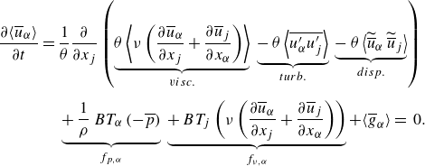 \begin{align} \frac {\partial \langle \overline {u}_\alpha \rangle }{ \partial t} = \; & \frac {1}{\theta } \frac {\partial }{\partial x_j} \left ( \underbrace { \theta \left \langle \nu \left ( \frac {\partial \overline {u}_\alpha }{\partial x_j} + \frac {\partial \overline {u}_j}{\partial x_\alpha } \right ) \right \rangle }_{visc.} \: \underbrace { - \: \theta \left \langle \overline {u^\prime _\alpha u^\prime _j} \right \rangle }_{turb.} \: \underbrace { - \: \theta \left \langle \widetilde {\overline {u}}_\alpha \, \widetilde {\overline {u}}_j \right \rangle }_{disp.} \right ) \nonumber\\[5pt] & \underbrace { + \: \frac {1}{\rho } \, BT_\alpha \left ( -\overline {p} \right ) }_{ f_{p,\alpha } } \: \underbrace { + \: BT_j \left ( \nu \left ( \frac {\partial \overline {u}_\alpha }{\partial x_j} + \frac {\partial \overline {u}_j}{\partial x_\alpha } \right ) \right ) }_{ f_{\nu ,\alpha } } + \langle \overline {g}_\alpha \rangle \, {= \, 0} . \end{align}
The obtained (A2) is consistent with the formulation chosen by Lian et al. (Reference Lian, Dallmann, Sonin, Roche, Packman, Liu and Wagner2021). In the budget equation of TKE and WKE, the full dissipation terms appear as
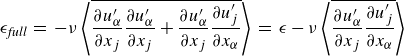 \begin{equation} \epsilon _{\textit{full}} \; = \; - \nu \left \langle \overline { \frac {\partial u^{\prime}_\alpha }{\partial x_j} \frac {\partial u^{\prime}_\alpha }{\partial x_j} + \frac {\partial u^{\prime}_\alpha }{\partial x_j} \frac {\partial u^{\prime}_j}{\partial x_\alpha } } \right \rangle \; = \; \epsilon - \nu \left \langle \overline { \frac {\partial u^{\prime}_\alpha }{\partial x_j} \frac {\partial u^{\prime}_j}{\partial x_\alpha } } \right \rangle \quad \, \end{equation}
and
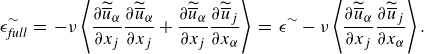 \begin{equation} \epsilon _{\textit{full}}^\sim \; = \; - \nu \left \langle \frac {\partial \widetilde {\overline {u}}_\alpha }{\partial x_j} \frac {\partial \widetilde {\overline {u}}_\alpha }{\partial x_j} + \frac {\partial \widetilde {\overline {u}}_\alpha }{\partial x_j} \frac {\partial \widetilde {\overline {u}}_j }{\partial x_\alpha } \right \rangle \; = \; \epsilon ^\sim - \nu \left \langle \frac {\partial \widetilde {\overline {u}}_\alpha }{\partial x_j} \frac {\partial \widetilde {\overline {u}}_j }{\partial x_\alpha } \right \rangle . \end{equation}
By the example of case M-300, figure 21 shows that the differences between pseudo dissipation and full dissipation are minor. For the TKE budget, this observation agrees with the statement of Pope (Reference Pope2000). Additionally, the small differences indicate that a pseudo dissipation formulation of the WKE budget is also justifiable.
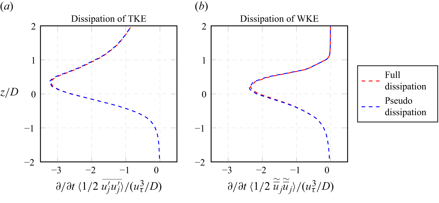
Figure 21. Minor differences between full dissipation and pseudo dissipation for both (a) TKE and (b) WKE. Case M-300 was used as an example. The friction velocity $u_\tau$
and the sphere diameter
$u_\tau$
and the sphere diameter $D$
are used for normalisation.
$D$
are used for normalisation.
Appendix B. Immersed boundary implementation
As pressure and viscous drag need to be evaluated, the method and accuracy of the immersed boundary implementation in MGLET deserve attention. Instead of feedback-forcing with a distributed forcing field (e.g. Goldstein, Handler & Sirovich Reference Goldstein, Handler and Sirovich1993), MGLET relies on a direct-forcing method, which comprises three steps within each Runge–Kutta substep (Peller Reference Peller2010; Sakai & Manhart Reference Sakai2020): (i) in an interpolation step, a stencil formulation is used to determine the velocities in cells intersected by solid surfaces. Under consideration of the velocities in neighbouring fluid-filled cells, the velocity in an intersected cell is computed such that the Dirichlet boundary condition at the position of the solid surface is fulfilled; (ii) in the flux correction step, the mass fluxes through the open faces of the intersected cell are computed. To ensure mass conservation at the immersed boundary, the divergence of the velocity field within the intersected cell is distributed among the neighbouring cells based on the open areas between the cells. That ensures that the rotation of the velocity field remains unchanged; (iii) the third step is the solution of a Poisson equation for the fluid-filled cells, which yields a pressure correction required to obtain a divergence-free flow field. As the velocity in the fluid-filled cells is updated, the fluxes through the faces of the intersected cell also change, such that steps (ii) and (iii) are iterated until the whole flow field is divergence-free. Only then, the next Runge-Kutta substep is entered.
We checked the solution of the pressure field around the immersed boundary for laminar flow around a cylinder by comparing it with a highly resolved simulation with a body-fitted finite volume method in OpenFOAM (Weller et al. Reference Weller, Tabor, Jasak and Fureby1998). Figure 22 shows the pressure fields for various grid resolutions. The flow within the periodic domain is driven by a volume force $g_x$
. Even at coarser resolutions, the immersed boundary yields a pressure field, which appears free of artificial distortions and visually similar to the solution on a body-fitted mesh. As the Poisson equation is only solved for the fluid-filled cells, no pressure values are available for the intersected cells in the immersed boundary case (best seen in figure 22
c). The pressure drag of the cylinder, which we evaluate as
$g_x$
. Even at coarser resolutions, the immersed boundary yields a pressure field, which appears free of artificial distortions and visually similar to the solution on a body-fitted mesh. As the Poisson equation is only solved for the fluid-filled cells, no pressure values are available for the intersected cells in the immersed boundary case (best seen in figure 22
c). The pressure drag of the cylinder, which we evaluate as $f_{\textit{p, IBM}} = \langle {\partial \overline { p }} / {\partial x} \rangle$
, converges with first-order accuracy, as shown by figure 23. The values of
$f_{\textit{p, IBM}} = \langle {\partial \overline { p }} / {\partial x} \rangle$
, converges with first-order accuracy, as shown by figure 23. The values of $f_{{p, \textit{IBM}}}$
at resolutions of 48 or more cells per diameter only deviate from the value
$f_{{p, \textit{IBM}}}$
at resolutions of 48 or more cells per diameter only deviate from the value $f_{\textit{p, BF}}$
of the body-fitted simulation by less than
$f_{\textit{p, BF}}$
of the body-fitted simulation by less than $0.7\,\%$
. The value
$0.7\,\%$
. The value $f_{\textit{p, BF}}$
is obtained by integrating
$f_{\textit{p, BF}}$
is obtained by integrating $(p \, {\boldsymbol{n}})$
over the cylinder surface, where
$(p \, {\boldsymbol{n}})$
over the cylinder surface, where ${\boldsymbol{n}}$
is the normal vector. Also, the value of the viscous drag
${\boldsymbol{n}}$
is the normal vector. Also, the value of the viscous drag $f_{{\nu, \textit{IBM}}} = \mu \langle {\partial /\partial x_j \, (\partial \overline { u }} / {\partial x_j}) \rangle$
agrees well with
$f_{{\nu, \textit{IBM}}} = \mu \langle {\partial /\partial x_j \, (\partial \overline { u }} / {\partial x_j}) \rangle$
agrees well with $f_{{\nu, \textit{BF}}}$
, which we obtain by computing the wall shear stress and integrating it over the cylinder surface of the body-fitted simulation. The values of
$f_{{\nu, \textit{BF}}}$
, which we obtain by computing the wall shear stress and integrating it over the cylinder surface of the body-fitted simulation. The values of $f_{{\nu, \textit{IBM}}}$
shown in figure 23(b) converge monotonically, whereas a convergence order cannot be specified.
$f_{{\nu, \textit{IBM}}}$
shown in figure 23(b) converge monotonically, whereas a convergence order cannot be specified.
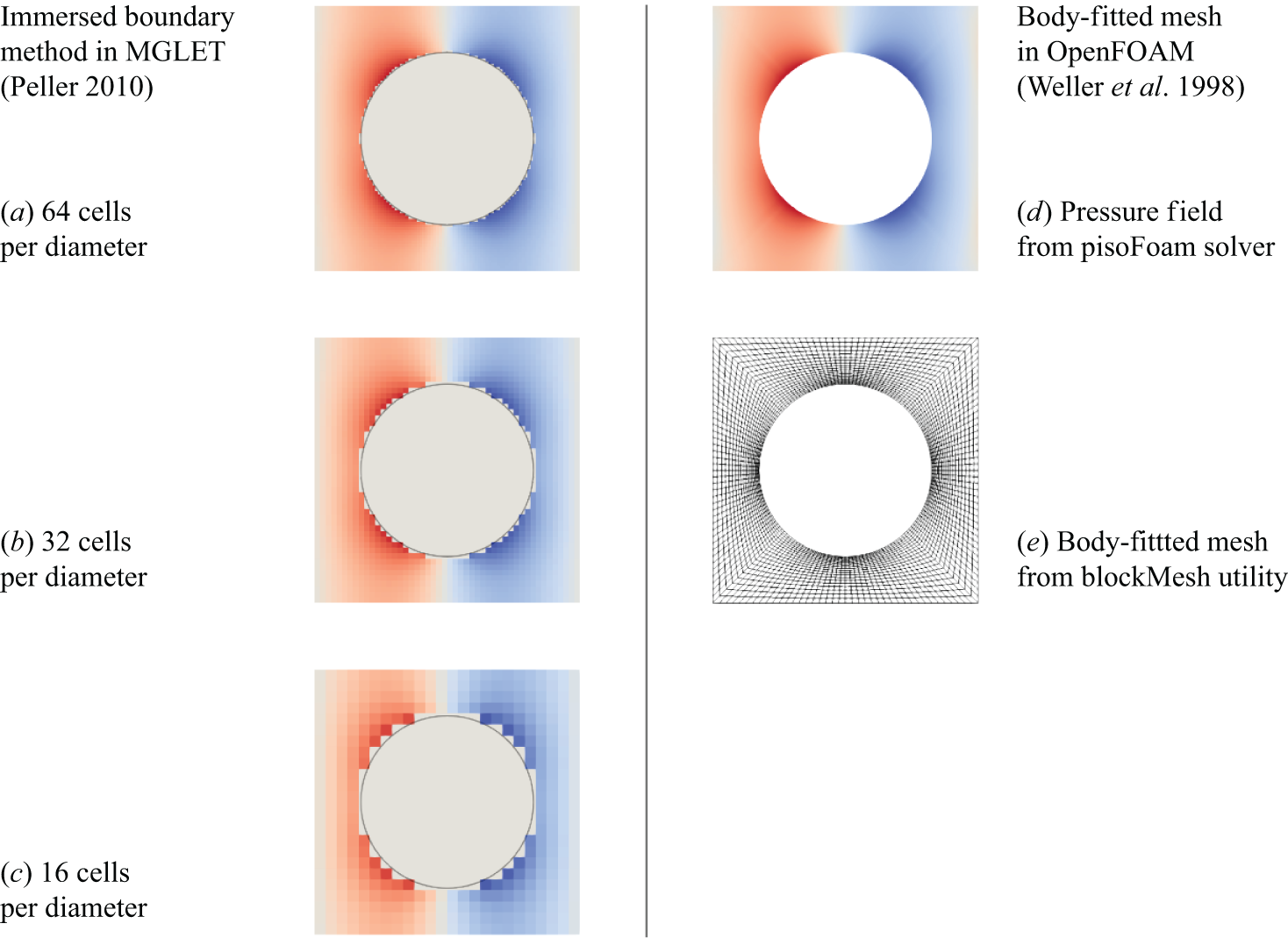
Figure 22. Pressure fields for laminar flow around cylinder in a two-dimensional $x$
-
$x$
- $y$
-periodic domain. Results from immersed boundary method at different resolutions are compared with computation on a body-fitted mesh.
$y$
-periodic domain. Results from immersed boundary method at different resolutions are compared with computation on a body-fitted mesh.
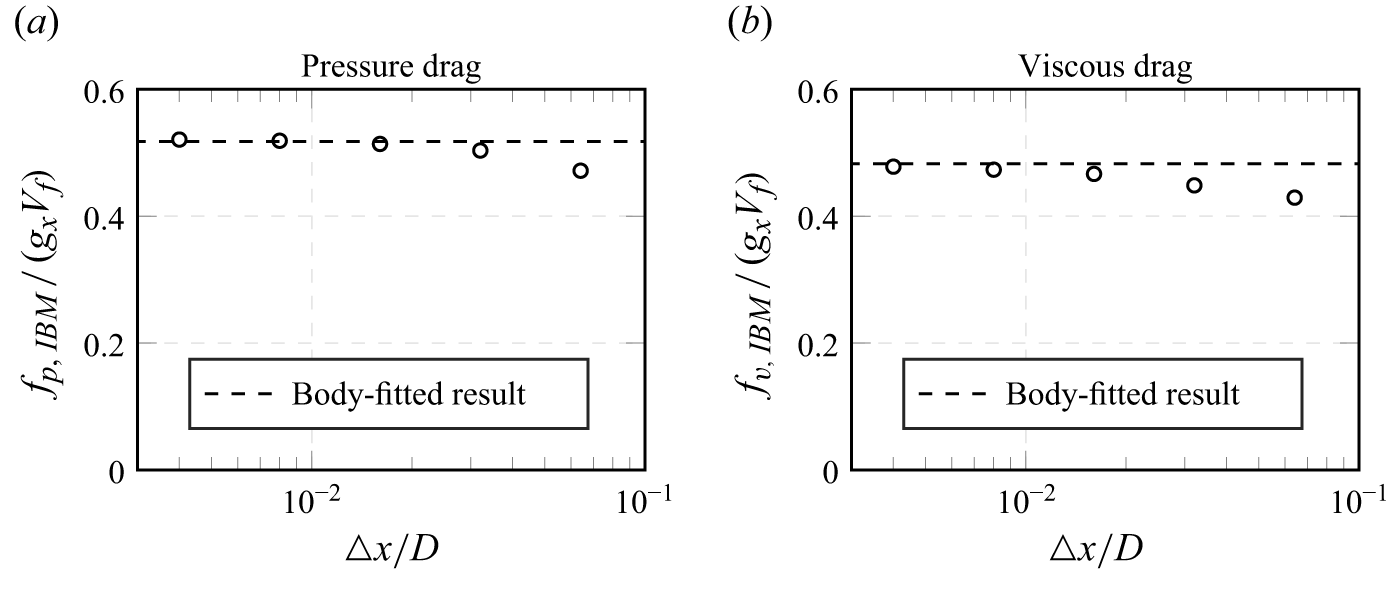
Figure 23. Convergence study of pressure and viscous drag determined by the immersed boundary method. The result from a simulation with a body-fitted mesh is given for comparison. The side length $\Delta x$
of the cubic cells is normalised by the cylinder diameter
$\Delta x$
of the cubic cells is normalised by the cylinder diameter $D$
. The drag is normalised by
$D$
. The drag is normalised by $(g_x V_{{f}})$
, where
$(g_x V_{{f}})$
, where $g_x$
is the driving volume force and
$g_x$
is the driving volume force and $V_{{f}}$
is the fluid volume. Accordingly, both normalised drags sum to unity.
$V_{{f}}$
is the fluid volume. Accordingly, both normalised drags sum to unity.
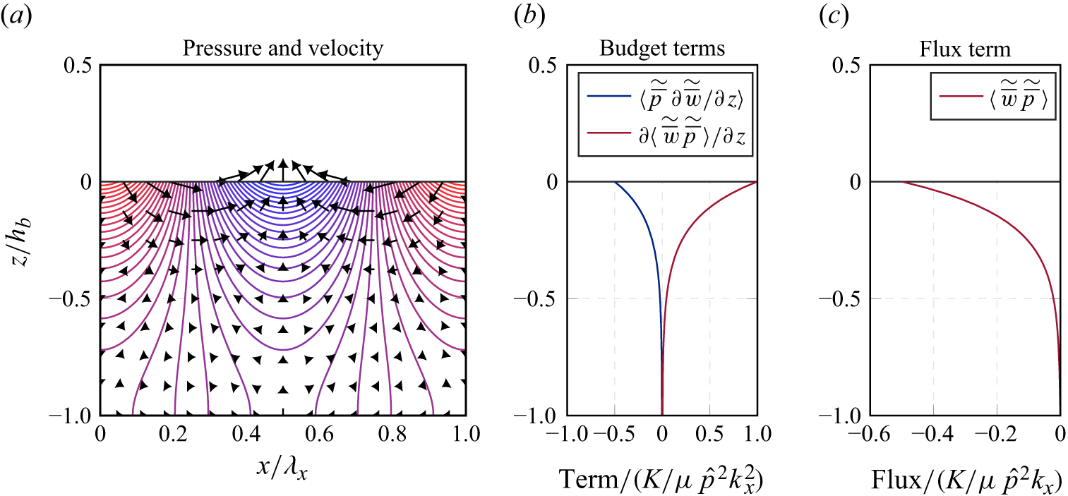
Figure 24. Qualitative visualisation of the analytical solution and normalised profiles of different terms. The analytical solution in panel (a) shows contour lines of the pressure field. The black arrows represent the flow from high pressure (red) to low pressure (blue). The budget terms in panel (b) represent the pressure redistribution term and the pressure transport term in the budget for $\partial / \partial t \langle \widetilde {\overline {w}} \, \widetilde {\overline {w}} \rangle / 2$
. The flux term in panel (c) represents the pressure-driven downward flux of
$\partial / \partial t \langle \widetilde {\overline {w}} \, \widetilde {\overline {w}} \rangle / 2$
. The flux term in panel (c) represents the pressure-driven downward flux of $\langle \widetilde {\overline {w}} \, \widetilde {\overline {w}} \rangle / 2$
. The permeability
$\langle \widetilde {\overline {w}} \, \widetilde {\overline {w}} \rangle / 2$
. The permeability $K$
, the dynamic viscosity
$K$
, the dynamic viscosity $\mu$
, the amplitude
$\mu$
, the amplitude $\hat {p}$
and the wavenumber
$\hat {p}$
and the wavenumber $k_x$
of the interfacial pressure variation are used for normalisation.
$k_x$
of the interfacial pressure variation are used for normalisation.
Appendix C. Pressure pumping scenario
We consider the following two-dimensional scenario, which resembles the case discussed by Elliott & Brooks (Reference Elliott and Brooks1997). The surface of a sediment bed with a permeability $K$
and a depth
$K$
and a depth $h_b$
lies at
$h_b$
lies at $z=0$
. On the sediment bed surface, a pressure field is prescribed as
$z=0$
. On the sediment bed surface, a pressure field is prescribed as
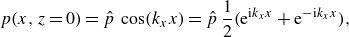 \begin{equation} p(x, z=0) = \hat {p} \, \cos (k_x x) = \hat {p} \, \frac {1}{2} \big(\mathrm{e}^{\mathrm{i} k_x x} + \mathrm{e}^{-\mathrm{i} k_x x} \big), \end{equation}
where $\hat {p} \gt 0$
is the amplitude of the regular cosine-shaped pressure variation and
$\hat {p} \gt 0$
is the amplitude of the regular cosine-shaped pressure variation and $k_x = 2 \pi / \lambda _x$
is the angular wavenumber of the regular spatial pressure variation with wavelength
$k_x = 2 \pi / \lambda _x$
is the angular wavenumber of the regular spatial pressure variation with wavelength $\lambda _x$
. For the interfacial boundary condition of (C1), an analytical solution for the pressure and flow field within the porous medium can be found, which fulfils Laplace’s equation for the pressure, while also
$\lambda _x$
. For the interfacial boundary condition of (C1), an analytical solution for the pressure and flow field within the porous medium can be found, which fulfils Laplace’s equation for the pressure, while also $w_D(z=-h_b) = 0$
is maintained, which corresponds to the bottom boundary of our simulation cases. Using solutions known in the context of Airy’s wave theory in combination with Darcy’s law, we obtain
$w_D(z=-h_b) = 0$
is maintained, which corresponds to the bottom boundary of our simulation cases. Using solutions known in the context of Airy’s wave theory in combination with Darcy’s law, we obtain
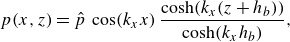 \begin{align} p(x, z) & = \hat {p} \, \cos (k_x x) \, \frac { \cosh ( k_x (z + h_b) ) }{ \cosh ( k_x h_b )} , \end{align}
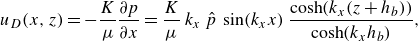 \begin{align} u_D(x, z) = -\frac {K}{\mu } \frac {\partial p}{\partial x} = \frac {K}{\mu } \, k_x \, \hat {p} \, \sin (k_x x) \, \frac { \cosh ( k_x (z + h_b) ) }{ \cosh ( k_x h_b )} , \end{align}
 \begin{align} w_D(x, z) = -\frac {K}{\mu } \frac {\partial p}{\partial z} = - \frac {K}{\mu } \, k_x \, \hat {p} \, \cos (k_x x) \, \frac { \sinh ( k_x (z + h_b) ) }{ \cosh ( k_x h_b )}. \end{align}
In (C2), (C3) and (C4), $\cosh (x) = ( e^x + e^{-x} ) / 2$
and
$\cosh (x) = ( e^x + e^{-x} ) / 2$
and $\sinh (x) = ( e^x - e^{-x} ) / 2$
represent the hyperbolic cosine and hyperbolic sine function, respectively. The subscript in
$\sinh (x) = ( e^x - e^{-x} ) / 2$
represent the hyperbolic cosine and hyperbolic sine function, respectively. The subscript in $u_D$
and
$u_D$
and $w_D$
identifies the velocity as Darcy velocities, which describe a divergence-free pressure-driven potential flow within the porous medium.
$w_D$
identifies the velocity as Darcy velocities, which describe a divergence-free pressure-driven potential flow within the porous medium.
The obtained analytical solution is represented in figure 24(a). We use the analytical solution to compute values of terms, which occur in the budget for $\langle \widetilde {\overline {w}} \, \widetilde {\overline {w}} \rangle$
. While no boundary terms occur in the idealised scenario, we obtain profiles for the redistribution term (see (2.11)) and the pressure transport term (see (2.12)). Also, the value of the pressure-induced WKE flux
$\langle \widetilde {\overline {w}} \, \widetilde {\overline {w}} \rangle$
. While no boundary terms occur in the idealised scenario, we obtain profiles for the redistribution term (see (2.11)) and the pressure transport term (see (2.12)). Also, the value of the pressure-induced WKE flux $J_{{pres}}^s = \langle \widetilde {\overline {w}} \, \widetilde {\overline {p}} \rangle$
can be obtained, such that
$J_{{pres}}^s = \langle \widetilde {\overline {w}} \, \widetilde {\overline {p}} \rangle$
can be obtained, such that
 \begin{align} \left \langle \widetilde {\overline {p}} \: \frac {\partial \widetilde {\overline {w}} }{\partial z} \right \rangle & = - \left ( \frac {K}{\mu } \hat {p}^2 k_x^2 \right ) \left ( \frac { \cosh ( k_x (z + h_b) ) }{ \cosh ( k_x h_b )} \right )^2 \frac {1}{\lambda _x} \int _0^{\lambda _x} \left ( \cos (k_x x) \right )^2 {\rm d}x \\[-5pt]\nonumber\end{align}
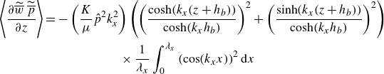 \begin{align} \left \langle \frac {\partial \widetilde {\overline {w}} \, \widetilde {\overline {p}} }{\partial z} \right \rangle & = - \left ( \frac {K}{\mu } \hat {p}^2 k_x^2 \right ) \left ( \left ( \frac { \cosh ( k_x (z + h_b) ) }{ \cosh ( k_x h_b )} \right )^2 + \left ( \frac { \sinh ( k_x (z + h_b) ) }{ \cosh ( k_x h_b )} \right )^2 \right )\nonumber\\&\qquad\qquad\qquad\times \frac {1}{\lambda _x} \int _0^{\lambda _x} \left ( \cos (k_x x) \right )^2 {\rm d}x\\[-5pt]\nonumber \end{align}
 \begin{align} \left \langle \widetilde {\overline {w}} \, \widetilde {\overline {p}} \right \rangle & = - \left ( \frac {K}{\mu } \hat {p}^2 k_x \right ) \frac { \cosh ( k_x (z + h_b) ) }{ \cosh ( k_x h_b )} \frac { \sinh ( k_x (z + h_b) ) }{ \cosh ( k_x h_b )} \frac {1}{\lambda _x} \int _0^{\lambda _x} \left ( \cos (k_x x) \right )^2 {\rm d}x \; . \end{align}
The expressions in (C5), (C6), (C7) assume that the domain length is a multiple of the wavelength $\lambda _x$
. Also, the equations show that the flux is expected to scale with
$\lambda _x$
. Also, the equations show that the flux is expected to scale with $K \hat {p}^2 k_x / \mu$
, while the budget terms are expected to scale with
$K \hat {p}^2 k_x / \mu$
, while the budget terms are expected to scale with $K \hat {p}^2 k_x^2 / \mu$
, if the sediment bed depth
$K \hat {p}^2 k_x^2 / \mu$
, if the sediment bed depth $h_b$
does not have a major influence. As shown in figure 24, the normalised quantities approach a zero value with increasing depth. The appearance of
$h_b$
does not have a major influence. As shown in figure 24, the normalised quantities approach a zero value with increasing depth. The appearance of $k_x$
in the
$k_x$
in the $z$
-dependent terms implies that this decay to zero happens closer to the sediment surface if the interfacial pressure variation has a higher wavenumber.
$z$
-dependent terms implies that this decay to zero happens closer to the sediment surface if the interfacial pressure variation has a higher wavenumber.


 Open access