


1. Introduction
Steady incoming flow past a smooth circular cylinder has been a classical problem in fluid mechanics owing to its fundamental significance and extensive practical applications (Zdravkovich Reference Zdravkovich1997). Although this canonical scenario is governed by a single dimensionless parameter, i.e. the Reynolds number Re (= UD/ $\nu$
, where U is the velocity of the incoming flow, D is the diameter of the cylinder and v is the kinematic viscosity of the fluid), several flow transitions and flow regimes have been observed (e.g. Williamson Reference Williamson1996; Zdravkovich Reference Zdravkovich1997). These include
$\nu$
, where U is the velocity of the incoming flow, D is the diameter of the cylinder and v is the kinematic viscosity of the fluid), several flow transitions and flow regimes have been observed (e.g. Williamson Reference Williamson1996; Zdravkovich Reference Zdravkovich1997). These include
-
(i) onset of two-dimensional (2-D) vortex shedding at Re ∼ 47, where the wake starts to display the classical primary (Kármán) vortex street;
-
(ii) onset of three-dimensionality at Re ∼ 190, where a relatively large-scale three-dimensional (3-D) wake structure (called mode A, with a spanwise period of ∼4D) develops between adjacent primary vortices;
-
(iii) a gradual transition from mode A to a finer-scale 3-D structure (called mode B, with a spanwise period less than 1D) over Re ∼ 230–260;
-
(iv) successive transitions to turbulence in the wake, the separating shear layer and the boundary layer at Re ∼ 270, 1200 and 2 × 10⁵, respectively.
The flow regimes/transitions and the associated flow characteristics and hydrodynamic/aerodynamic behaviours of the body may be altered via various flow control techniques (Choi, Jeon & Kim Reference Carmo, Sherwin, Bearman and Willden2008). Examples of passive control include attaching splitter plates to the cylinder (Roshko Reference Roshko1954, Reference Roshko1961; Apelt, West & Szewczyk Reference Apelt, West and Szewczyk1973; Kwon & Choi Reference Williamson1996), adding small control cylinders (Strykowski & Sreenivasan Reference Strykowski and Sreenivasan1990; Wang, Zhang & Wu Reference Wang, Zhang and Wu2006; Marquet, Sipp & Jacquin Reference Carmo, Sherwin, Bearman and Willden2008) or other small bodies (Prasad & Williamson Reference Zdravkovich1997) near the main cylinder, changing the surface roughness on the cylinder (Shih et al. Reference Shih, Wang, Coles and Roshko1993), etc. Examples of active control include applying various blowing/suction patterns on the cylinder surface (Dong, Triantafyllou & Karniadakis Reference Carmo, Sherwin, Bearman and Willden2008; Poncet et al. Reference Carmo, Sherwin, Bearman and Willden2008; Feng & Wang Reference Feng and Wang2010), oscillating the cylinder in line with the incident flow (Xu, Zhou & Wang Reference Wang, Zhang and Wu2006), transverse to the incident flow (Williamson & Roshko Reference Williamson and Roshko1988; Carberry, Sheridan & Rockwell Reference Blackburn, Marques and Lopez2005) or about its axis (Tokumaru & Dimotakis Reference Tokumaru and Dimotakis1991), among many others. Although the flow control techniques may differ between one another, common purposes include (i) suppression of vortex shedding, (ii) suppression/mitigation of the fluctuating lift force and the associated vortex-induced vibration (VIV) (e.g. Cui, Feng & Hu Reference Cui, Feng and Hu2022; Sun et al. Reference Cui, Feng and Hu2022) and acoustic noise (e.g. You et al. Reference You, Choi, Choi and Kang1998; Duan & Wang Reference Duan and Wang2021) and (iii) drag force reduction.
One of the simplest yet effective flow control techniques in achieving the above-mentioned three purposes is to attach a splitter plate to the rear end of the cylinder. This arrangement delays the interaction between the two shear layers separated from the two sides of the cylinder and affects the vortex formation pattern (Roshko Reference Roshko1955). The basic scenario of a rear-attached splitter plate has also been extended upon by using e.g. a detached plate in the wake (Roshko Reference Roshko1954; Ozono Reference Ozono1999; Hwang, Yang & Sun Reference Hwang, Yang and Sun2003; Serson et al. Reference Serson, Meneghini, Carmo, Volpe and Gioria2014), dual rear-attached plates (Wang et al. Reference Wang, Bao, Zhou, Zhu, Ping, Han, Serson and Xu2019), a rear-attached wavy (Zhu & Liu Reference Zhu and Liu2020) or flexible plate (Duan & Wang Reference Duan and Wang2021), a front-attached plate (Qiu et al. Reference Serson, Meneghini, Carmo, Volpe and Gioria2014; Chutkey, Suriyanarayanan & Venkatakrishnan Reference Chutkey, Suriyanarayanan and Venkatakrishnan2018; Gao et al. Reference Wang, Bao, Zhou, Zhu, Ping, Han, Serson and Xu2019), both front- and rear-attached plates (Qiu et al. Reference Serson, Meneghini, Carmo, Volpe and Gioria2014; Gao et al. Reference Wang, Bao, Zhou, Zhu, Ping, Han, Serson and Xu2019) and by using a rear-attached splitter plate for bluff bodies other than a circular cylinder, e.g. a square cylinder (Ali, Doolan & Wheatley Reference Ali, Doolan and Wheatley2011; Chauhan et al. Reference Chutkey, Suriyanarayanan and Venkatakrishnan2018), an elliptic cylinder (Soumya & Prakash Reference Soumya and Prakash2017) or a half-ellipse with a blunt trailing edge (Bearman 1965). Most of the above-mentioned scenarios produced various levels of reductions in the mean drag and/or fluctuating lift, as well as alterations in the vortex shedding frequency.
The present study focuses on the most canonical scenario of a circular cylinder with a rear-attached splitter plate. Early studies by Roshko (Reference Roshko1954, Reference Roshko1961) examined both subcritical and transcritical Re values, and showed that a splitter plate was effective in reducing the mean drag and base pressure on the cylinder. For example, at a subcritical Re of 1.45 × 10⁴, the use of a splitter plate with a non-dimensional length L/D = 5 resulted in a marked reduction in the mean drag coefficient from 1.15 to 0.72 (Roshko Reference Roshko1954,Reference Roshko1961). Similar drag reduction behaviours were also observed by most of the experimental studies summarised in table 1. In addition, Gao et al. (Reference Wang, Bao, Zhou, Zhu, Ping, Han, Serson and Xu2019) also reported a significant reduction in the fluctuating lift on the cylinder with L/D up to 2.
Table 1. Experimental studies for flow past a circular cylinder with a rear-attached splitter plate.
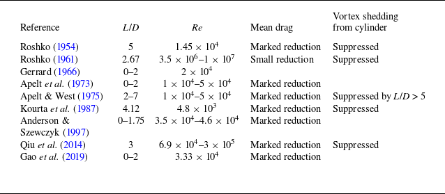
As for the influence on the vortex shedding, Apelt & West (Reference Apelt and West1975) examined a range of L/D = 2–7 and found that, for L/D> 5, vortex shedding from the cylinder was suppressed by the plate, and instead vortex shedding developed from the trailing edge of the plate. This phenomenon was also reported by Roshko (Reference Roshko1961), Kourta et al. (Reference Kourta, Boisson, Chassaing and Ha Minh1987) and Qiu et al. (Reference Serson, Meneghini, Carmo, Volpe and Gioria2014), where relatively long plates (L/D ≥ 2.67) were tested. In contrast, Gerrard (Reference Gerrard1966), Apelt et al. (Reference Apelt, West and Szewczyk1973), Anderson & Szewczyk (Reference Zdravkovich1997) and Gao et al. (Reference Wang, Bao, Zhou, Zhu, Ping, Han, Serson and Xu2019) examined cases with L/D ≤ 2 and did not report suppression of vortex shedding from the cylinder. Instead, Gerrard (Reference Gerrard1966), Apelt et al. (Reference Apelt, West and Szewczyk1973) and Anderson & Szewczyk (Reference Zdravkovich1997) focused on the influence of L/D on the vortex shedding frequency, and found that the shedding frequency was altered in a non-monotonic fashion with the increase in L/D.
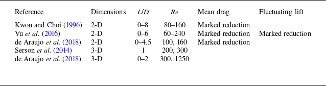
While the experimental studies summarised in table 1 generally focused on the range of Re ≳ O(104), previous numerical studies, summarised in table 2, focused on Re ∼ O(102–103) instead. Specifically, Kwon & Choi (Reference Williamson1996), Vu, Ahn & Hwang (Reference Jiang, Cheng, Draper, An and Tong2016) and de Araujo, Schettini & Silvestrini (Reference Chutkey, Suriyanarayanan and Venkatakrishnan2018) conducted 2-D numerical simulations and quantified the influence of Re and L/D on the vortex shedding frequency and the marked reductions in the mean drag and fluctuating lift coefficients. In addition, Serson et al. (Reference Serson, Meneghini, Carmo, Volpe and Gioria2014) and de Araujo et al. (Reference Chutkey, Suriyanarayanan and Venkatakrishnan2018) extended the numerical simulations to a few 3-D cases, and examined the influence of Re and L/D on the vortex shedding frequency (but not on the drag or lift coefficient). Although the 3-D results were limited to only a few cases on the vortex shedding frequency, they suggested that the flow three-dimensionality played a significant role in altering the hydrodynamic characteristics.
Table 2. Two- and three-dimensional numerical studies for flow past a circular cylinder with a rear-attached splitter plate.
In addition, the Floquet analyses of Serson et al. (Reference Serson, Meneghini, Carmo, Volpe and Gioria2014) and Wang et al. (Reference Wang, Bao, Zhou, Zhu, Ping, Han, Serson and Xu2019), for the cases of a detached splitter plate (with L/D = 1 and a gap between the cylinder and the plate being G/D = 0.5–3) and dual-attached splitter plates, respectively, showed that different types of placement of plates in the cylinder wake may significantly alter the critical Re for the 3-D wake transition and the 3-D wake instability modes.
However, for the more canonical scenario of an attached splitter plate, there has been no investigation in the literature on the onset of 3-D wake transition, (linear) 3-D wake instability modes, (nonlinear) 3-D wake structures and the significant influence of the three-dimensionality on the hydrodynamic characteristics (other than merely a few cases on the vortex shedding frequency).
To address these knowledge gaps, the present study carries out a systematic investigation on the influence of an attached splitter plate on the 2-D and 3-D wake transitions, 3-D wake instability modes, 3-D wake structures and the influence of the three-dimensionality on the hydrodynamic characteristics (e.g. the mean drag and fluctuating lift on the cylinder and the splitter plate). A relatively large parameter space of Re = 10–480 and L/D = 0–6 is examined, covering both the 2-D and 3-D wake transition regimes.
2. Numerical model
2.1. Numerical method
In the present study, the flow was solved by the direct numerical simulation (DNS) framework embedded in the open-source code Nektar $\texttt{++}$
(Cantwell et al. Reference Cantwell2015). The governing equations for the flow were the continuity and incompressible Navier–Stokes equations
$\texttt{++}$
(Cantwell et al. Reference Cantwell2015). The governing equations for the flow were the continuity and incompressible Navier–Stokes equations
 \begin{align} \mathbf{\nabla }\cdot \boldsymbol{u}=0 , \\[-26pt] \nonumber \end{align}
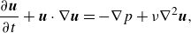 \begin{align} \frac{\partial \boldsymbol{u}}{\partial t}+\boldsymbol{u}\cdot \mathbf{\nabla }\boldsymbol{u}=-\mathbf{\nabla }p+\nu \nabla ^{2}\boldsymbol{u} , \\[6pt] \nonumber \end{align}
where
u
(
x
, t) = (u
x
, u
y
, u
z
)(x, y, z, t) is the velocity field, u
x
, u
y
and u
y
denote the velocity components in the streamwise (x), transverse (y) and spanwise (z) directions, respectively, p(
x
, t) is the kinematic pressure (pressure divided by fluid density), t is time and ν is kinematic viscosity of the fluid. Equations (2.1) and (2.2) were solved by the unsteady Navier–Stokes solver embedded in Nektar $\texttt{++}$
, together with the use of a velocity correction scheme (Karniadakis, Israeli & Orszag Reference Tokumaru and Dimotakis1991), a second-order implicit–explicit time-integration scheme and a continuous Galerkin projection. A high-order spectral element method (Karniadakis & Sherwin Reference Blackburn, Marques and Lopez2005) was used for the x–y plane. For the 3-D DNS, a Fourier expansion was used in the geometrically homogeneous spanwise direction (Karniadakis Reference Strykowski and Sreenivasan1990).
$\texttt{++}$
, together with the use of a velocity correction scheme (Karniadakis, Israeli & Orszag Reference Tokumaru and Dimotakis1991), a second-order implicit–explicit time-integration scheme and a continuous Galerkin projection. A high-order spectral element method (Karniadakis & Sherwin Reference Blackburn, Marques and Lopez2005) was used for the x–y plane. For the 3-D DNS, a Fourier expansion was used in the geometrically homogeneous spanwise direction (Karniadakis Reference Strykowski and Sreenivasan1990).
2.2. Computational domain and mesh
A hexahedral computational domain, as sketched in figure 1(a), was used for the 3-D DNS, while the corresponding domain in the x–y plane was used for the 2-D DNS. A circular cylinder was placed at (x, y) = (0, 0), while a splitter plate of zero thickness, as highlighted in blue, was attached to the rear end of the cylinder. The boundary conditions for the computational domain included a uniform velocity (u x , u y , u z ) = (U, 0, 0) at the inlet and transverse sides, a zero normal velocity gradient at the outlet and a no-slip condition at the cylinder and plate surfaces. The boundary conditions for the pressure included a reference value of zero at the outlet, and a high-order Neumann condition (Karniadakis et al. Reference Tokumaru and Dimotakis1991) at all other boundaries. For the 3-D DNS, periodic boundary conditions were employed at the two boundaries perpendicular to the cylinder span. The internal flow followed an impulsive start.
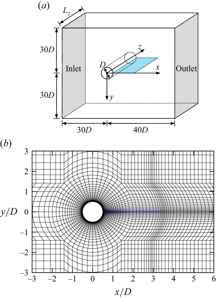
Figure 1. Computational domain and mesh for the case of flow past a circular cylinder with a splitter plate attached: (a) schematic model of the computational domain (not to scale), and (b) close-up view of the macro-element mesh near the cylinder–plate system for the case L/D = 3. The splitter plate is highlighted in blue.
The computational mesh in the x–y plane consisted of approximately 10 000 macro-elements. Figure 1(b) shows a close-up view of the macro-element mesh near the cylinder–plate system for the case L/D = 3. Local mesh refinements were made around the cylinder and plate. The cylinder surface was discretised with 64 macro-elements, while the height of the first layer of elements next to the cylinder was 0.00553D. At the trailing edge of the splitter plate, the element size was locally refined to 0.0667D × 0.0320D. To capture detailed wake evolution along the streamwise direction, a relatively high resolution was used in the wake region by specifying the streamwise size of the elements at the wake centreline (y = 0) increasing linearly from 0.167D at x/D = (L/D + 1) to 0.5D at x/D = 30.5. The macro-elements were then subdivided using high-order Lagrange polynomials on the Gauss–Lobatto–Legendre points for the quadrilateral expansions. Fifth-order polynomials (N
p
= 5) were used for the 2-D DNS and Floquet analysis, while fourth-order polynomials (N
p
= 4) were used for the 3-D DNS. The non-dimensional time-step size $\Delta$
tU/D was 0.0025 for N
p
= 5 and 0.004 for N
p
= 4, which corresponded to a Courant–Friedrichs–Lewy limit of no more than 0.6.
$\Delta$
tU/D was 0.0025 for N
p
= 5 and 0.004 for N
p
= 4, which corresponded to a Courant–Friedrichs–Lewy limit of no more than 0.6.
Table 3. Results of the 2-D mesh dependence study for the case L/D = 4 and Re = 480.
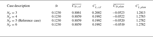
2.3. Mesh convergence
A mesh dependence study was performed based on the case L/D = 4 and Re = 480 (the largest Re considered in the present study). Firstly, 2-D DNSs were used to examine the adequacy of the mesh resolution in the x–y plane. In additional to the reference case with N p = 5, three variation cases with N p = 3, 4 and 6 were computed. Table 3 lists the numerical results predicted by different mesh resolutions. The Strouhal number (St) for the cylinder–plate system and the drag and lift coefficients (C D and C L ) on the cylinder/plate are calculated as
 \begin{align} St=\frac{f_{L}D}{U} , \\[-26pt] \nonumber \end{align}
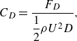 \begin{align} C_{D}=\frac{F_{D}}{\dfrac{1}{2}\rho U^{2}D} , \\[-26pt] \nonumber \end{align}
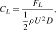 \begin{align} C_{L}=\frac{F_{L}}{\dfrac{1}{2}\rho U^{2}D} , \\[-9pt] \nonumber \end{align}
where f
L
is the peak frequency obtained from the fast Fourier transform of the time history of C
L
, while F
D
and F
L
are the drag and lift forces on the cylinder/plate (per unit span length). The time-averaged drag and lift coefficients are denoted $\overline{C_{D}}$
and
$\overline{C_{D}}$
and $\overline{C_{L}}$
, respectively. The root-mean-square lift coefficient (
$\overline{C_{L}}$
, respectively. The root-mean-square lift coefficient ( $C'_{L}$
) is calculated as
$C'_{L}$
) is calculated as
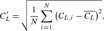 \begin{align} C'_{L}=\sqrt{\frac{1}{N}\sum _{i=1}^{N}\left(C_{L,i}-\overline{C_{L}}\right)^{2}} , \end{align}
where N is the data length in the time history of C L . The forces on the cylinder and plate are distinguished by the subscripts ‘cyl’ and ‘plate’, respectively. As shown in table 3, the hydrodynamic forces predicted with N p ≥ 4 are practically unchanged, which suggested that the mesh resolution in the x–y plane was adequate.
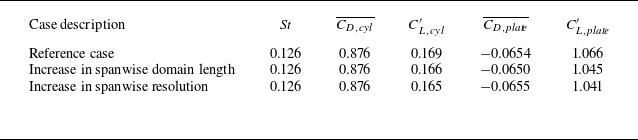
The 3-D mesh dependence study focused on the adequacy of the spanwise domain length (L z /D = 16) and spanwise resolution (128 Fourier planes) used for the reference case. Two variation cases were considered.
-
(i) Variation case 1: the spanwise domain length was increased by 1.5 times to L z /D = 24, while the spanwise resolution was unchanged (i.e. 192 Fourier planes for L z /D = 24); and.
-
(ii) variation case 2: the spanwise resolution was increased by 1.5 times through using 192 Fourier planes over L z /D = 16.
For each 3-D case, at least 400 non-dimensional time units (defined as $t^{*}$
= tU/D) were used to wash out the initial transients. After that, at least another 500 time units were used for the statistics. Table 4 lists the hydrodynamic coefficients calculated with the three cases. The close agreement in the coefficients suggested that the spanwise domain length and resolution used by the reference case were adequate.
$t^{*}$
= tU/D) were used to wash out the initial transients. After that, at least another 500 time units were used for the statistics. Table 4 lists the hydrodynamic coefficients calculated with the three cases. The close agreement in the coefficients suggested that the spanwise domain length and resolution used by the reference case were adequate.
Table 4. Results of the 3-D mesh dependence study for the case L/D = 4 and Re = 480.
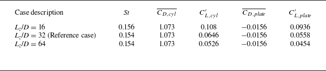
For L/D ≤ 0.5 and L/D ≥ 4, the most unstable spanwise wavelengths of the 3-D wake instability modes predicted by the Floquet analysis (to be presented in § 4) were no more than 4.11D, such that the use of L z /D = 16 for the 3-D DNS accommodated at least three spanwise periods of the unstable mode, which was deemed adequate (Jiang, Cheng & An Reference Soumya and Prakash2017). For L/D = 1–3, however, the most unstable wavelengths for the 3-D wake instability modes were more than 10D, such that an increased L z /D of 32 was used (together with the use of 256 Fourier planes so as to keep the spanwise resolution unchanged). The adequacy of L z /D = 32 was examined based on the case L/D = 1 and Re = 180 (the smallest Re for the 3-D DNS of L/D = 1, where the unstable wavelength was the largest). Table 5 lists the hydrodynamic coefficients obtained with L z /D = 16, 32 and 64, which suggested that the use of L z /D = 32 was adequate.
Table 5. Results of the L z dependence study for the case L/D = 1 and Re = 180.
3. Onset of vortex shedding
For an isolated circular cylinder, the 2-D vortex shedding emerges as a result of a Hopf bifurcation at a critical Re (Re cr2D) of approximately 47 (e.g. Henderson Reference Zdravkovich1997). Similarly, figure 2 quantifies the Re cr2D values for a circular cylinder with a no-slip splitter plate of L/D = 0–6. The Re cr2D for each L/D is determined by the method introduced in Appendix A. As shown in figure 2, with the increase in L/D, the Re cr2D value increases monotonically (but not linearly). Since the Re cr2D–L/D relationship is not reported in the literature, the present Re cr2D–L/D relationship is compared with the Re cr2D–L/D relationship for a slightly different scenario by Sahu, Furquan & Mittal (Reference Wang, Bao, Zhou, Zhu, Ping, Han, Serson and Xu2019), whose rear-attached splitter plate had a finite thickness of 0.2D (in contrast to a zero thickness plate for the present study). Although the results do not match quantitatively due to the use of different plate thicknesses, the Re cr2D–L/D relationship by Sahu et al. (Reference Wang, Bao, Zhou, Zhu, Ping, Han, Serson and Xu2019) also showed a monotonic but nonlinear increase in Re cr2D, which is qualitatively similar to the variation trend of the present Re cr2D–L/D relationship.
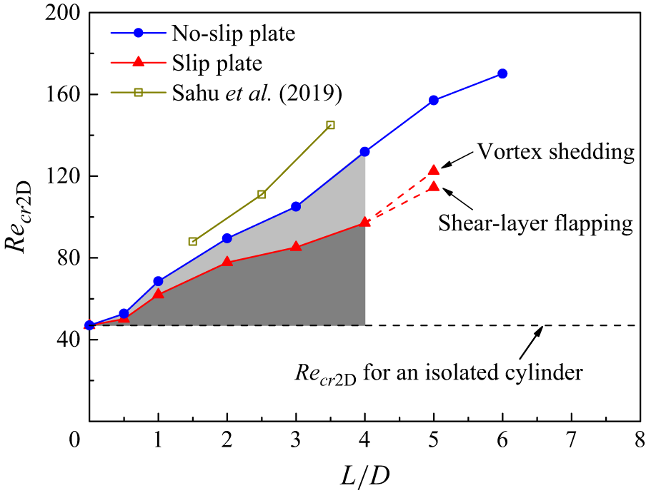
Figure 2. Critical Re for the onset of vortex shedding for a circular cylinder with a rear-attached splitter plate of either no-slip or slip boundary condition.
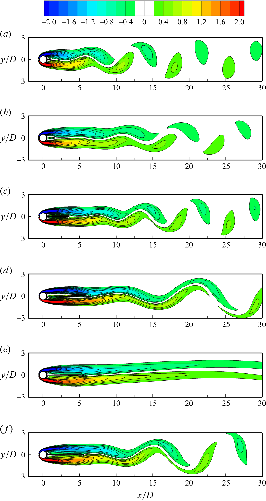
Figure 3. Instantaneous spanwise vorticity fields at Re slightly above Re cr2D: (a) (L/D, Re) = (0.5, 60), (b) (L/D, Re) = (1, 70), (c) (L/D, Re) = (3, 110), (d) (L/D, Re) = (6, 180), (e) (L/D, Re) = (5, 120) with a slip splitter plate and (f) (L/D, Re) = (5, 130) with a slip splitter plate.
For the present scenario with different L/D values, figure 3(a–d) illustrates instantaneous spanwise vorticity ( $\omega_z$
) fields at Re slightly above Re
cr2D, where
$\omega_z$
) fields at Re slightly above Re
cr2D, where $\omega_z$
is defined in a non-dimensional form as
$\omega_z$
is defined in a non-dimensional form as
 \begin{align} \omega _{z}=\left(\frac{\partial u_{y}}{\partial x}-\frac{\partial u_{x}}{\partial y}\right)\frac{D}{U} . \end{align}
With the increase in L/D, the streamwise location of vortex shedding is pushed further downstream. Physically, the splitter plate is a boundary with a no-penetration condition (u y = 0) and a no-slip condition (u x = 0). The two conditions induce an increase in Re cr2D with increase in L/D through two effects.
-
(i) Effect of the no-penetration condition. The shear layers separated from the two sides of the cylinder are gradually weakened with distance downstream (e.g. the vorticity in the shear layer gradually reduces with distance downstream). When the instability of the separating shear layers and the formation and shedding of the vortices are restricted by the no-penetration condition of the plate and are forced to develop further downstream with increasing L/D, the separating shear layers at the location of vortex shedding are further weakened. Therefore, an increased Re cr2D is required for the shear layers to gain more strength to roll up into vortices.
-
(ii) Effect of the no-slip condition. The shear layers developed on the two sides of the no-slip plate are of opposite sign of vorticity to the shear layers separated from the cylinder (figure 3 a–d) and further weaken the latter, which induces a further increased Re cr2D for the generation of vortices.
To quantitatively reveal individual contribution of the no-penetration condition and no-slip condition, we introduce a specifically designed case with a splitter plate using a slip boundary condition (∂u x /∂y = 0, u y = 0 and a high-order Neumann condition for the pressure). By replacing the no-slip plate with the slip plate, the no-slip condition is removed whereas the no-penetration condition is preserved. The Re cr2D values for the cases with no-slip and slip plates are both shown in figure 2. For the slip plate cases, the focus is placed on L/D ≤ 4, because for L/D = 5 an additional flow regime is observed in between of the steady regime (Re ≲ 110) and the vortex shedding regime (Re ≳ 125; figure 3 f), over which the separating shear layers display a low-frequency (∼1/6 times the vortex shedding frequency) periodic flapping behaviour, without generation of vortices (figure 3 e). As shown in figure 2, the cases with the slip plate (the red curve) divide the increase in Re cr2D (the shaded area) into two parts. The darker area represents the increase in Re cr2D induced by the no-penetration condition, while the lighter area represents the further increase in Re cr2D induced by the no-slip condition. The contribution by the no-penetration condition is more significant (which accounts for ∼60 %–70 % of the increase in Re cr2D), while the no-slip condition also plays an important role.
It is worth noting that, in the present context, the onset/suppression of vortex shedding quantified in figure 2 is with respect to the entire cylinder–plate system, which is different from the ‘suppression’ of vortex shedding from the cylinder and a transfer of vortex shedding to the trailing edge of the plate reported by Roshko (Reference Roshko1961), Apelt & West (Reference Apelt and West1975), Kourta et al. (Reference Kourta, Boisson, Chassaing and Ha Minh1987) and Qiu et al. (Reference Serson, Meneghini, Carmo, Volpe and Gioria2014) with Re ≳ O(104) and relatively long plate lengths (L/D ≥ 2.67). When the vortex shedding is directed away from the cylinder by the plate, the effect of vortex shedding on the cylinder is weakened but not fully eliminated. This feature is reflected by a reduction (but not suppression) in the fluctuating lift on the cylinder shown later on in figure 17(b). The ‘suppression’ of vortex shedding from the cylinder reported by the experimental studies of Roshko (Reference Roshko1961), Apelt & West (Reference Apelt and West1975), Kourta et al. (Reference Kourta, Boisson, Chassaing and Ha Minh1987) and Qiu et al. (Reference Serson, Meneghini, Carmo, Volpe and Gioria2014) may be better interpreted as a mitigation of the effect of vortex shedding on the cylinder.
4. Three-dimensional wake transition
Beyond a specific critical Re for the onset of three-dimensionality (denoted Re cr3D), 3-D flow structures develop in the wake and may alter the hydrodynamic forces on the cylinder and the plate. In this section, the 3-D wake transitions for L/D = 0–6 are examined through both Floquet stability analysis and 3-D DNS. The Floquet analysis, which follows that reported by Barkley & Henderson (Reference Williamson1996), is used to determine the Re cr3D value for the onset of three-dimensionality and to identify the 3-D wake instability modes. Figure 4 summarises the critical Re and spanwise wavelength (λ) for the 3-D wake instability modes determined by the Floquet analysis. With the increase in L/D, the first 3-D wake instability mode observed at Re cr3D changes in the sequence of (i) mode A for L/D = 0–0.5, (ii) mode AL for L/D = 1, (iii) mode BL for L/D = 2–3 and (iv) mode QP3 for L/D = 4–6. For modes AL and BL, the first letter represents a spatio-temporal symmetry pattern similar to that for mode A or B for an isolated cylinder, i.e.
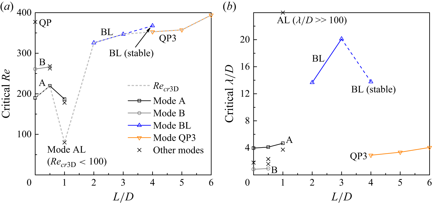
Figure 4. Floquet analysis results for various L/D conditions: (a) critical Re for the 3-D wake instability modes, and (b) critical λ/D for these modes.
Symmetry pattern of the mode A type
 \begin{align} \omega _{x}\left(x,y,z,t\right)=-\omega _{x}\left(x,-y,z,t+T/2\right) .\end{align}
Symmetry pattern of the mode B type
 \begin{align} \omega _{x}\left(x,y,z,t\right)=\omega _{x}\left(x,-y,z,t+T/2\right) , \end{align}
where $\omega_x$
is the streamwise vorticity defined in a non-dimensional form as
$\omega_x$
is the streamwise vorticity defined in a non-dimensional form as
 \begin{align} \omega _{x}=\left(\frac{\partial u_{z}}{\partial y}-\frac{\partial u_{y}}{\partial z}\right)\frac{D}{U} , \end{align}
and T is the vortex shedding period. The second letter, L, indicates a long spanwise wavelength (of more than ten times larger than that for the conventional mode A or B for an isolated cylinder, see figure 4 b). In addition, three quasi-periodic (QP) modes are observed for the cases with a splitter plate, which are named QP1, QP2 (for L/D = 0.5) and QP3 (for L/D = 4–6). It is worth noting that the Re cr3D values and 3-D wake instability modes summarised in figure 4 for the present scenario with an attached splitter plate are significantly different from those reported by Serson et al. (Reference Serson, Meneghini, Carmo, Volpe and Gioria2014) and Wang et al. (Reference Wang, Bao, Zhou, Zhu, Ping, Han, Serson and Xu2019) for the scenarios with other types of placement of plates in the cylinder wake (a detached splitter plate and dual-attached splitter plates, respectively), which demonstrates the necessity of the present investigation.
In addition to the Floquet analysis, 3-D DNSs are used to reveal the unstable modes and overall wake structures for the real 3-D flows, and to obtain statistically stationary hydrodynamic forces over the 3-D wake transition regimes. For each 3-D case, the statistical time period spans at least 400 non-dimensional time units, after discarding an initial transient period of at least another 400 time units.
Owing to the significant variations in the 3-D wake instability modes and the critical Re and λ/D values with L/D (figure 4), the Floquet analysis and 3-D DNS results for L/D = 0–0.5, 1, 2–3 and 4–6 are presented separately in §§ 4.1–4.4, respectively.
4.1. Three-dimensional results for L/D = 0–0.5
The 3-D results for L/D = 0.5 are relatively similar to those for an isolated cylinder, and are therefore reported first. Figure 5(a) shows the dependence of the dominant Floquet multiplier $ \mu $
on the spanwise wavenumber
$ \mu $
on the spanwise wavenumber $ \beta $
(= 2π/λ) for several Re values, where four wake instability modes are detected. Based on the
$ \beta $
(= 2π/λ) for several Re values, where four wake instability modes are detected. Based on the $| \mu |$
–
$| \mu |$
– $ \beta $
relationships predicted at a number of Re values, the neutral instability curves for the four modes are mapped out in figure 5(b).
$ \beta $
relationships predicted at a number of Re values, the neutral instability curves for the four modes are mapped out in figure 5(b).
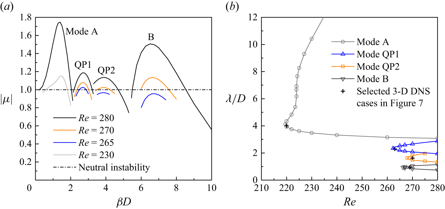
Figure 5. Floquet analysis results for L/D = 0.5: (a) the $| \mu |$
–
$| \mu |$
– $ \beta $
relationships for several Re values, and (b) the neutral instability curves for the 3-D wake instability modes.
$ \beta $
relationships for several Re values, and (b) the neutral instability curves for the 3-D wake instability modes.
Figure 6 shows the streamwise perturbation vorticity fields for the four modes. The perturbation patterns shown in figure 6(a,d), which display opposite signs and same sign for the two sides of the wake centreline, respectively, agree with the patterns of modes A and B for an isolated cylinder (see e.g. Carmo, Meneghini & Sherwin Reference Feng and Wang2010). In addition, the critical spanwise wavelengths for modes A and B, which are determined at the left tip of the corresponding neutral curve (figure 5b ) as 4.11D and 0.94D, respectively, remain similar to those of modes A and B for an isolated cylinder (e.g. 3.97D and 0.83D by Posdziech & Grundmann (Reference Posdziech and Grundmann2001)). As for the critical Re values for modes A and B, the present results of 219.6 and 266.2 are slightly larger than those for an isolated cylinder (e.g. 190.2 and 261.0 by Posdziech & Grundmann (Reference Posdziech and Grundmann2001)), which suggests that a short splitter plate is able to delay the onset of three-dimensionality slightly.
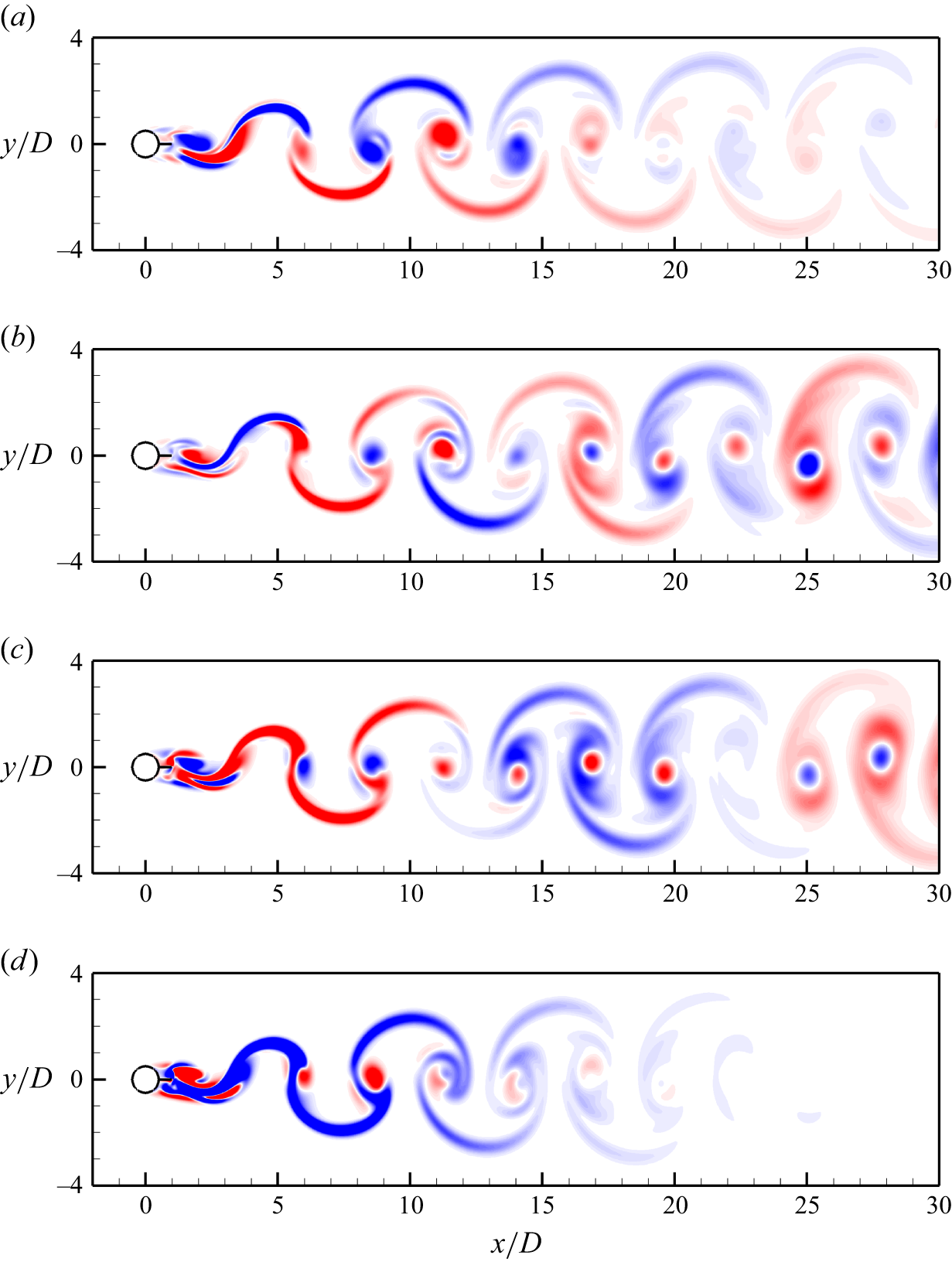
Figure 6. Streamwise perturbation vorticity fields for the case (L/D, Re) = (0.5, 280): (a) mode A predicted at $ \beta $
D = 1.4, (b) mode QP1 predicted at
$ \beta $
D = 1.4, (b) mode QP1 predicted at $ \beta $
D = 2.7, (c) mode QP2 predicted at
$ \beta $
D = 2.7, (c) mode QP2 predicted at $ \beta $
D = 3.9 and (d) mode B predicted at
$ \beta $
D = 3.9 and (d) mode B predicted at $ \beta $
D = 6.5. Red and blue denote positive and negative vorticity values, respectively.
$ \beta $
D = 6.5. Red and blue denote positive and negative vorticity values, respectively.
In addition to the synchronous modes A and B, two QP modes are observed for L/D = 0.5 (figure 5). The streamwise perturbation vorticity fields for the two QP modes display irregular arrangement of both signs at each side of the wake centreline (figure 6 b,c). The critical Re values for the two QP modes (262.3 and 267.9) are much smaller than that for the QP mode of an isolated cylinder (e.g. 377 by Blackburn, Marques & Lopez (Reference Blackburn, Marques and Lopez2005)).
To further confirm the existence of the four unstable modes shown in figures 5 and 6, 3-D DNSs are used to reveal their 3-D structures. The 3-D DNSs are performed with Re and L z (= λ) close to the left tip of each neutral instability curve (marked by + in figure 5 b), such that the wake is only unstable to one mode, and the 3-D structure is relatively regular. Figure 7 shows the streamwise and spanwise vorticity structures corresponding to the four modes. The modes A and B structures shown in figure 7(a,d) display out-of-phase and in-phase sequences between the neighbouring streamwise vortices along the streamwise direction, respectively, which are consistent with those for the modes A and B structures for an isolated cylinder (see e.g. Williamson Reference Williamson1996). In contrast, the two QP structures display travelling waves moving in the spanwise direction, which are similar to the QP structure for an isolated cylinder reported by Blackburn et al. (Reference Blackburn, Marques and Lopez2005). The travelling waves for the QP modes explain the irregular patterns of the streamwise perturbation vorticity fields shown in figure 6(b,c).
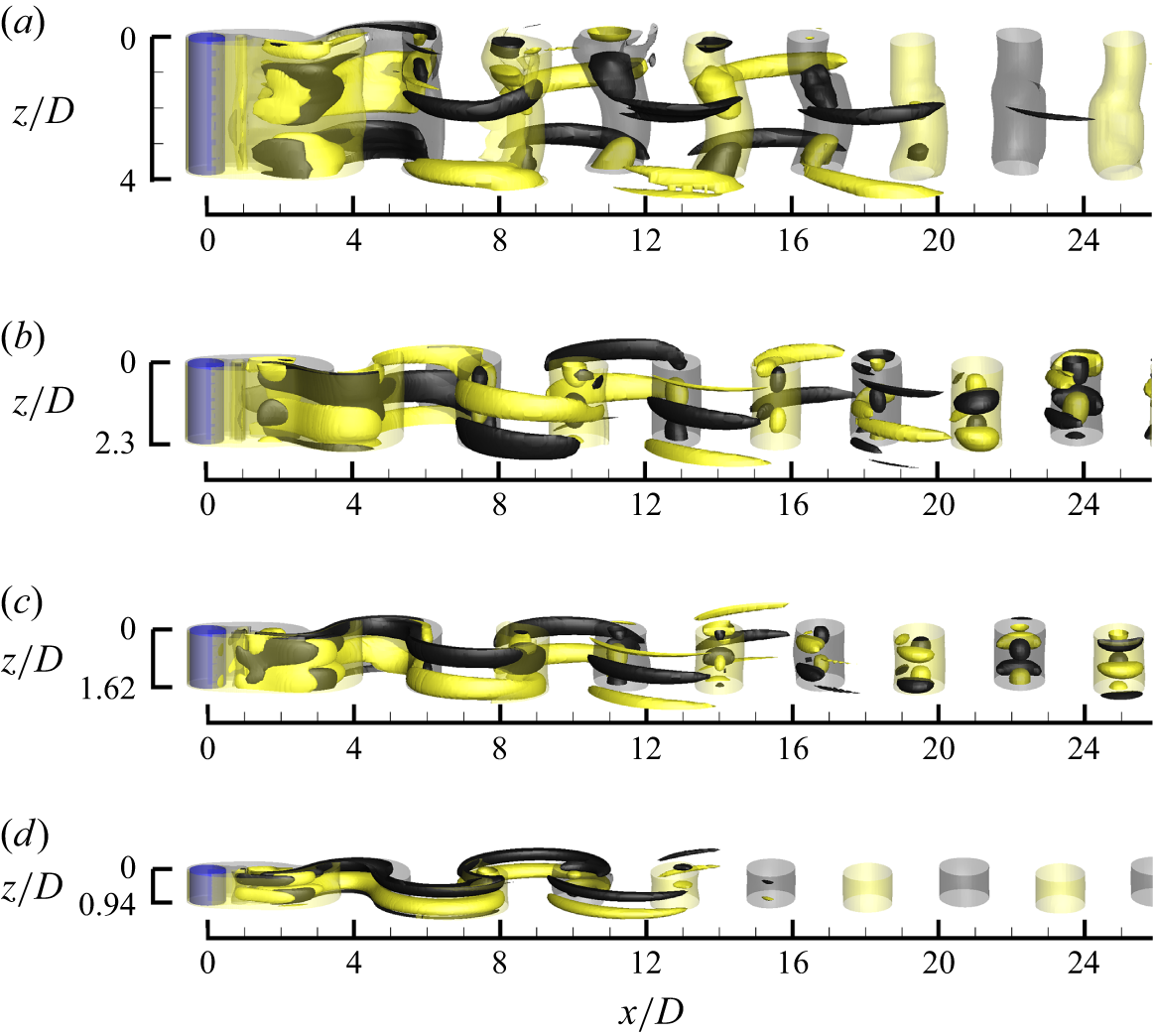
Figure 7. Instantaneous vorticity fields for the 3-D wake instability modes observed for L/D = 0.5: (a) mode A structure at (Re, L
z
/D) = (220, 4.0), (b) mode QP1 structure at (Re, L
z
/D) = (263, 2.3), (c) mode QP2 structure at (Re, L
z
/D) = (270, 1.62) and (d) mode B structure at (Re, L
z
/D) = (269, 0.94). The translucent iso-surfaces represent spanwise vortices with | $\omega_z$
| = 0.5, while the opaque iso-surfaces represent streamwise vortices with |
$\omega_z$
| = 0.5, while the opaque iso-surfaces represent streamwise vortices with | $\omega_x$
| = 0.5, 0.1, 0.1 and 0.2 for panels (a–d), respectively. Dark grey and light yellow denote positive and negative vorticity values, respectively. The flow is from left to right past the cylinder on the left.
$\omega_x$
| = 0.5, 0.1, 0.1 and 0.2 for panels (a–d), respectively. Dark grey and light yellow denote positive and negative vorticity values, respectively. The flow is from left to right past the cylinder on the left.
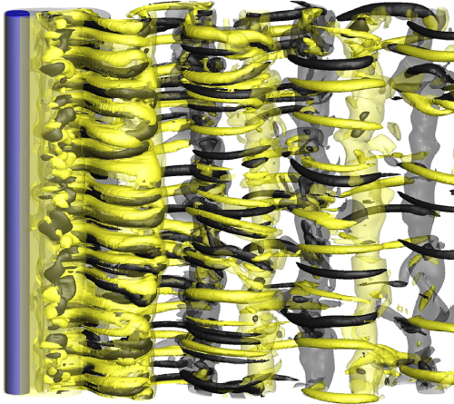
To allow for complex interactions among the wake instability modes, 3-D DNSs are also performed with a sufficiently long spanwise domain length of L z /D = 16, which may accommodate four spanwise periods of the longest wavelength mode. As Re exceeds Re cr3D of 219.6, the first flow regime observed at Re = 220 and 230 is represented by the development of four spanwise periods of ordered mode A structure (figure 8 a), followed by the development of vortex dislocations and disordered mode A structure in the fully developed flow (figure 8 b). With the increase in Re to 240 and 260, a mode swapping (over time) between the relatively large-scale mode A structure and the finer-scale structures (figure 8 c) is observed. Owing to the influence of the mode A streamwise vortices and their influence back onto the spanwise vortices (i.e. the base flow), the finer-scale structures appear in the real 3-D flow earlier than their critical Re values predicted by the Floquet analysis (at Re ≥ 262.3). As Re increases from 240 to 260, the dominant wake pattern changes from the mode A structure to the finer-scale structures. A difference to the mode swapping between modes A and B for the case of an isolated cylinder (Williamson Reference Williamson1996) is that, for the case of L/D = 0.5, it is difficult to determine the types of modes for the finer-scale structures, since mode B and the two QP modes become unstable to the base flow at very similar Re values (figure 5 b). Beyond the mode swapping regime, the present DNSs show that the wakes of Re = 280–400 are always represented by the small-scale structures (e.g. figure 8 d). Regardless of the types of modes for the small-scale structures, over this flow regime the wake becomes increasingly chaotic and turbulent.
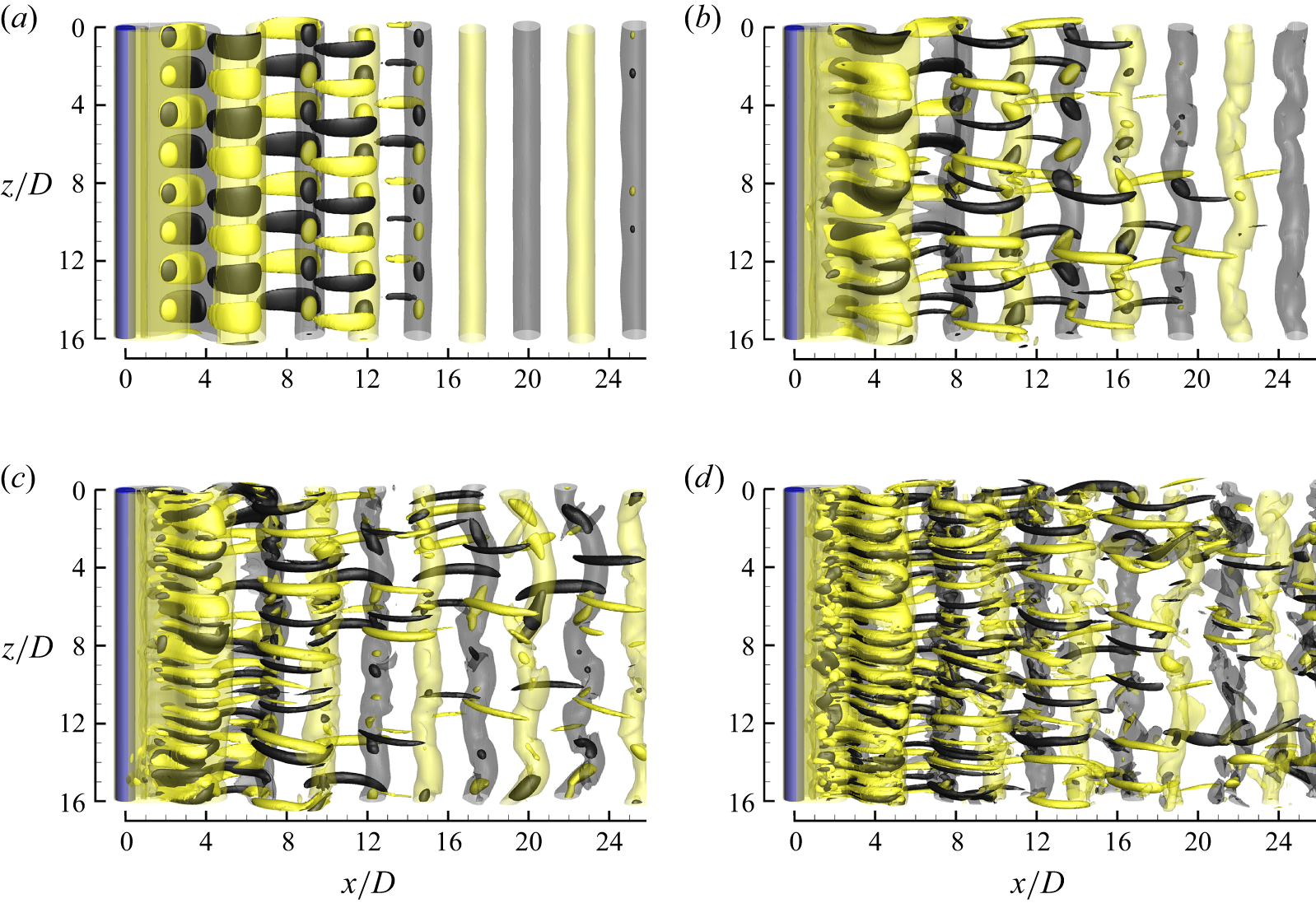
Figure 8. Instantaneous vorticity fields for L/D = 0.5: (a) Re = 220 (ordered mode A structure before evolution to dislocations), (b) Re = 220 (disordered mode A structure in the fully developed flow), (c) Re = 260 (disordered finer-scale structure) and (d) Re = 400 (increasingly disordered finer-scale structure). The translucent iso-surfaces represent spanwise vortices with | $\omega_z$
| = 0.5, while the opaque iso-surfaces represent streamwise vortices with |
$\omega_z$
| = 0.5, while the opaque iso-surfaces represent streamwise vortices with | $\omega_x$
| = 0.07, 0.7, 0.7 and 1.0 for panels (a–d), respectively. Dark grey and light yellow denote positive and negative vorticity values, respectively. The flow is from left to right past the cylinder on the left.
$\omega_x$
| = 0.07, 0.7, 0.7 and 1.0 for panels (a–d), respectively. Dark grey and light yellow denote positive and negative vorticity values, respectively. The flow is from left to right past the cylinder on the left.
4.2. Three-dimensional results for L/D = 1
The 3-D results for L/D = 1 are completely different from those for L/D = 0 and 0.5. Figure 9(a) shows the first three unstable modes for L/D = 1 predicted by the Floquet analysis, while figure 10 shows the streamwise perturbation vorticity fields for the three modes. For L/D = 1, the first unstable mode is a long wavelength mode AL with a spatio-temporal symmetry pattern of the mode A type (figure 10
a). Figure 9(b) shows the neutral instability curve for mode AL. Unlike conventional 3-D wake instability modes which are unstable over a finite range of spanwise wavelengths (cf. e.g. figure 5), mode AL is marginally unstable towards $ \beta $
D → 0 (figure 9
a), i.e. λ/D → ∞ (figure 9
b). The critical Re for the onset of mode AL is well below 100, while the unstable wavelength λ/D is of the order of 102. The emergence of the unconventional mode AL for L/D = 1 coincides with the strong influence of a splitter plate of L/D = 1 in altering the base flow by directing the vortex formation downstream of the plate.
$ \beta $
D → 0 (figure 9
a), i.e. λ/D → ∞ (figure 9
b). The critical Re for the onset of mode AL is well below 100, while the unstable wavelength λ/D is of the order of 102. The emergence of the unconventional mode AL for L/D = 1 coincides with the strong influence of a splitter plate of L/D = 1 in altering the base flow by directing the vortex formation downstream of the plate.
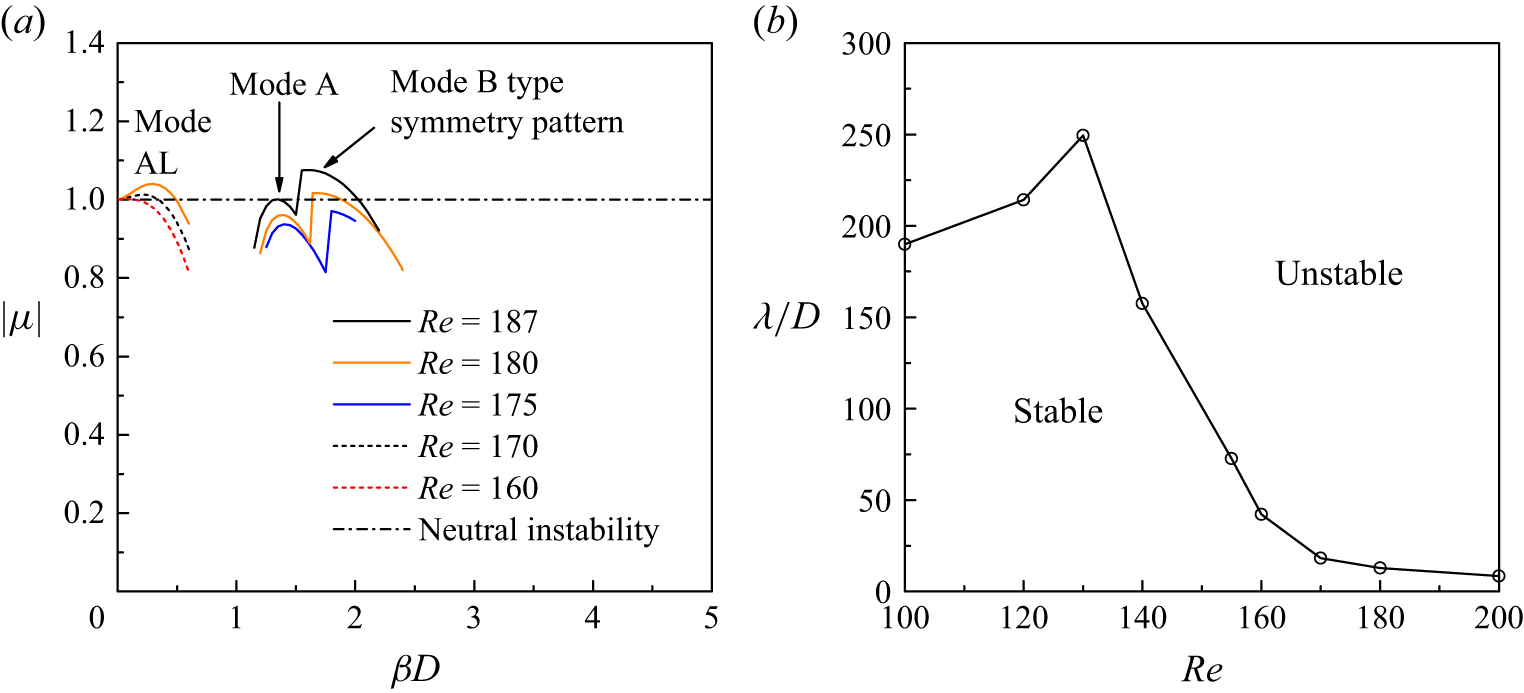
Figure 9. Floquet analysis results for L/D = 1: (a) the $| \mu |$
–
$| \mu |$
– $ \beta $
relationships for several Re values, and (b) the neutral instability curve for mode AL.
$ \beta $
relationships for several Re values, and (b) the neutral instability curve for mode AL.
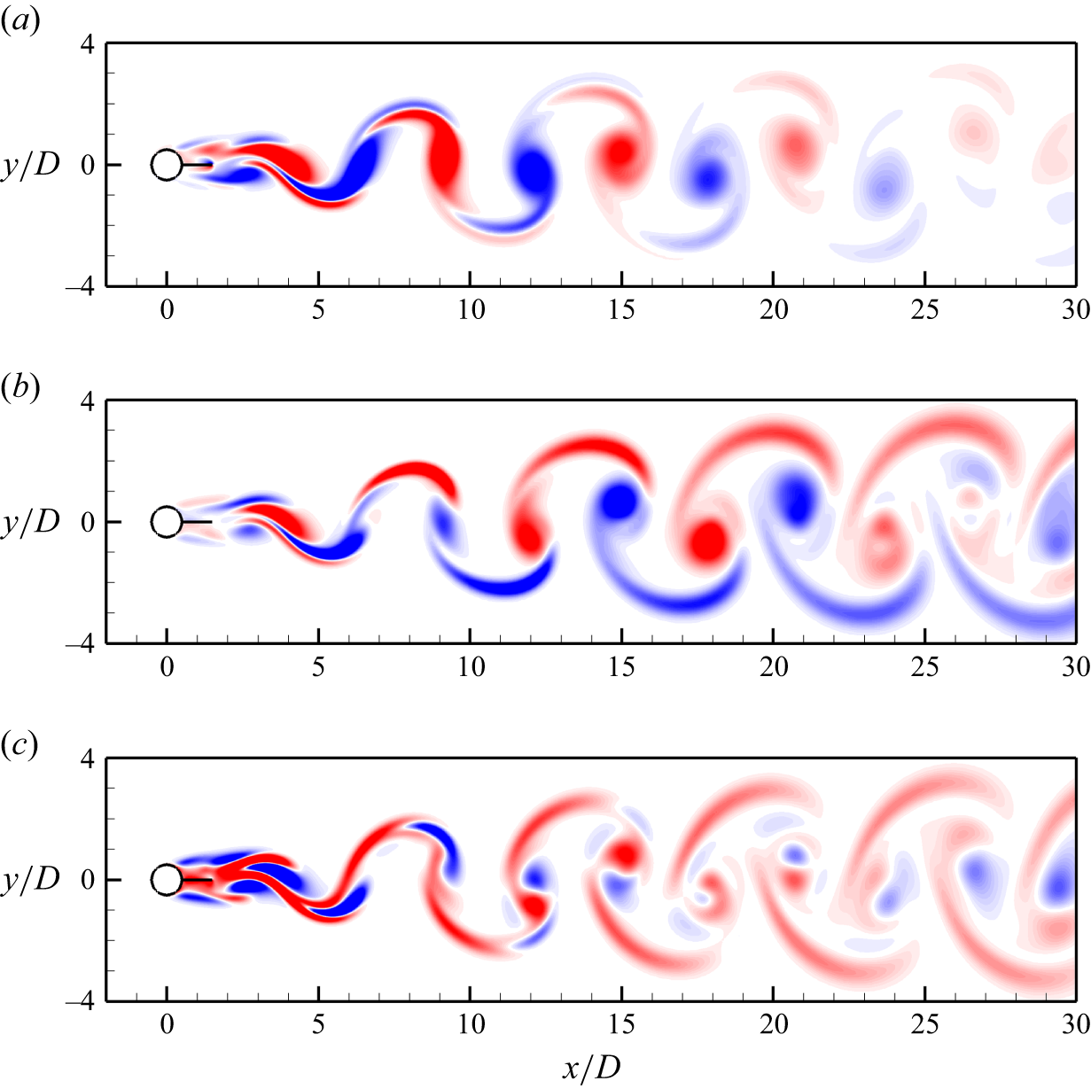
Figure 10. Streamwise perturbation vorticity fields for the case (L/D, Re) = (1, 180): (a) mode AL predicted at $ \beta $
D = 0.3, (b) mode A predicted at
$ \beta $
D = 0.3, (b) mode A predicted at $ \beta $
D = 1.44 and (c) a synchronous mode of mode B type symmetry pattern predicted at
$ \beta $
D = 1.44 and (c) a synchronous mode of mode B type symmetry pattern predicted at $ \beta $
D = 1.68. Red and blue denote positive and negative vorticity values, respectively.
$ \beta $
D = 1.68. Red and blue denote positive and negative vorticity values, respectively.
In addition to mode AL, two additional synchronous modes are observed in figure 9(a), and their spatio-temporal symmetry patterns are of the mode A and B types, respectively (figure 10 b,c). Nevertheless, the perturbation pattern shown in figure 10(c) is somewhat different from that of the conventional mode B shown in figure 6(d). Although the three synchronous modes observed in figure 9 may not represent a complete set of the unstable modes over the wake transition regimes, Floquet analyses are limited to Re ≤ 200, because (i) above this the real 3-D flow is expected to be governed by complex interactions of multiple modes rather than a single mode, and (ii) the 2-D base flow becomes aperiodic at Re > 240, which prohibits a strict Floquet analysis.
To reveal complex mode interactions in the real 3-D flows, 3-D DNSs are performed with L z /D = 32. Although the onset of three-dimensionality is well below Re = 100, the 3-D DNSs are performed for Re ≥ 180, because
-
(i) In addition to mode AL, other modes identified by the Floquet analysis become unstable at Re ≳ 180 (figure 9 a). Therefore, in the real 3-D flow, mode interactions may be expected at Re ≳ 180.
-
(ii) With the increase in Re, the critical λ/D for the mode AL instability decreases significantly (figure 9 b), such that a reduced L z may be used for the DNS. At Re = 180, the critical λ/D for the mode AL instability (= 12.8) is well below L z /D = 32 used for the DNS. The adequacy of L z /D = 32 for the present DNS is validated in table 5 by an L z dependence study at Re = 180.
Figure 11 illustrates the wake structures predicted by the 3-D DNS with L z /D = 32. At Re = 180, the wake is represented by one spanwise period of mode AL (figure 11 a). The periodicity of the mode AL structure is confirmed by an additional 3-D DNS with L z /D = 64, where two spanwise periods of mode AL are observed (not shown). With the increase in Re to 190, a mixture of mode AL and the smaller-scale mode A (e.g. over z/D ∼ 16–21 in figure 11 b) is observed. The emergence of mode A in the real 3-D flow is consistent with the mode A instability predicted by the Floquet analysis at the critical Re of 186.8. With the further increase in Re to 200 and beyond, mode AL is no longer observed. The wake is dominated by disordered smaller-scale (λ/D ∼ 5) mode A type structures at Re = 200 (figure 11 c) and even finer-scale structures (λ/D ∼ 1) over Re = 240–400 (figure 11 d).
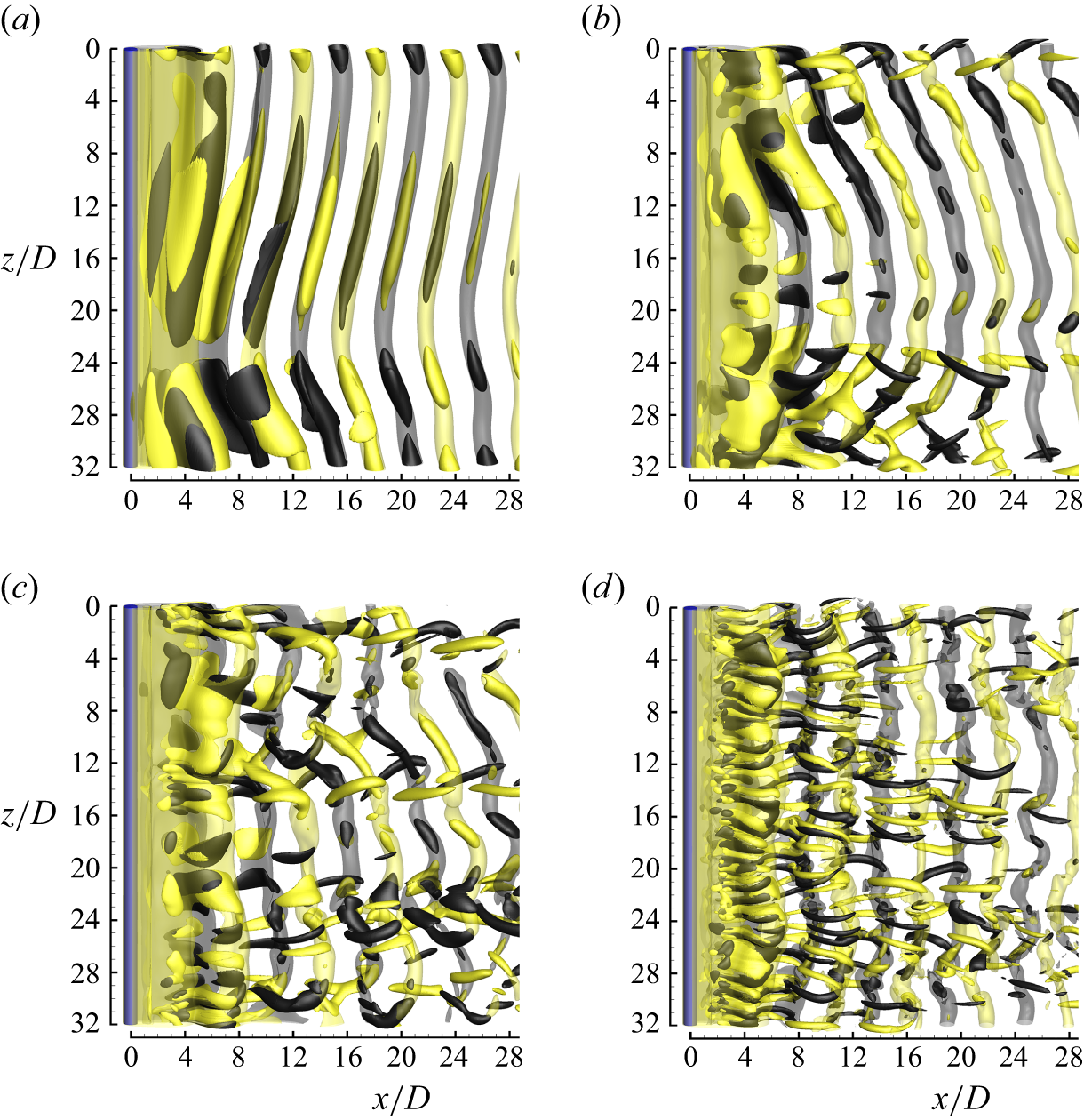
Figure 11. Instantaneous vorticity fields for L/D = 1: (a) Re = 180 (one spanwise period of mode AL), (b) Re = 190 (a mixture of modes AL and A), (c) Re = 200 (disappearance of mode AL) and (d) Re = 280 (chaotic fine-scale structures). The translucent iso-surfaces represent spanwise vortices with | $\omega_z$
| = 0.5, while the opaque iso-surfaces represent streamwise vortices with |
$\omega_z$
| = 0.5, while the opaque iso-surfaces represent streamwise vortices with | $\omega_x$
| = 0.15, 0.35, 0.4 and 0.7 for panels (a–d), respectively.
$\omega_x$
| = 0.15, 0.35, 0.4 and 0.7 for panels (a–d), respectively.
4.3. Three-dimensional results for L/D = 2–3
As L/D increases from 1 to 2, the onset of three-dimensionality is significantly delayed to Re
cr3D > 320 (figure 4
a). For L/D = 2 and 3, mode BL is the only unstable mode up to at least Re = 400, and its neutral instability curve is presented in figure 12(b). Figure 12(a) also reveals a marginally stable mode for L/D = 2 (not observed for L/D = 3). Based on a curve fitting of the peak $| \mu |$
values for Re = 300–360, the largest
$| \mu |$
values for Re = 300–360, the largest $| \mu |$
value for this mode, i.e.
$| \mu |$
value for this mode, i.e. $| \mu |$
= 0.998 at Re = 331, is confirmed to be less than 1.0.
$| \mu |$
= 0.998 at Re = 331, is confirmed to be less than 1.0.
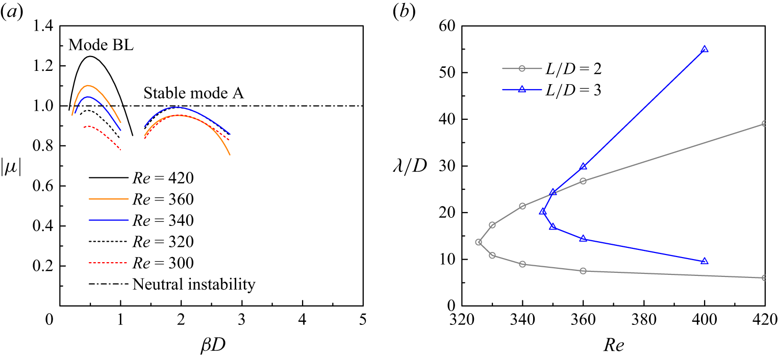
Figure 12. Floquet analysis results for L/D = 2 and 3: (a) the $| \mu |$
–
$| \mu |$
– $ \beta $
relationships for L/D = 2, and (b) the neutral instability curves for the 3-D wake instability mode, i.e. mode BL.
$ \beta $
relationships for L/D = 2, and (b) the neutral instability curves for the 3-D wake instability mode, i.e. mode BL.
Figure 13 shows the streamwise perturbation vorticity fields for mode BL and the stable mode. The symmetry pattern for mode BL (figure 13 a) is similar to that of the conventional mode B observed for L/D = 0–0.5 (e.g. figure 6 d). However, mode BL differs from mode B in that (i) its spanwise wavelength is more than ten times larger than that for mode B (figure 4 b), and (ii) the neighbouring streamwise vortices along the streamwise direction are disconnected (figure 13 a). As for the stable mode shown in figure 13(b), its pattern resembles that of the conventional mode A (figure 6 a), such that it is termed stable mode A in figure 12(a). It is also noticed in figure 13 that the 3-D modes are mainly developed based on the interactions of the neighbouring primary vortices that occur downstream of the splitter plate, rather than based on the primary vortices initially generated on the two sides of the plate. This phenomenon may contribute to the delayed 3-D wake transition for L/D ≥ 2, as the strength of the primary vortices decays with distance downstream.
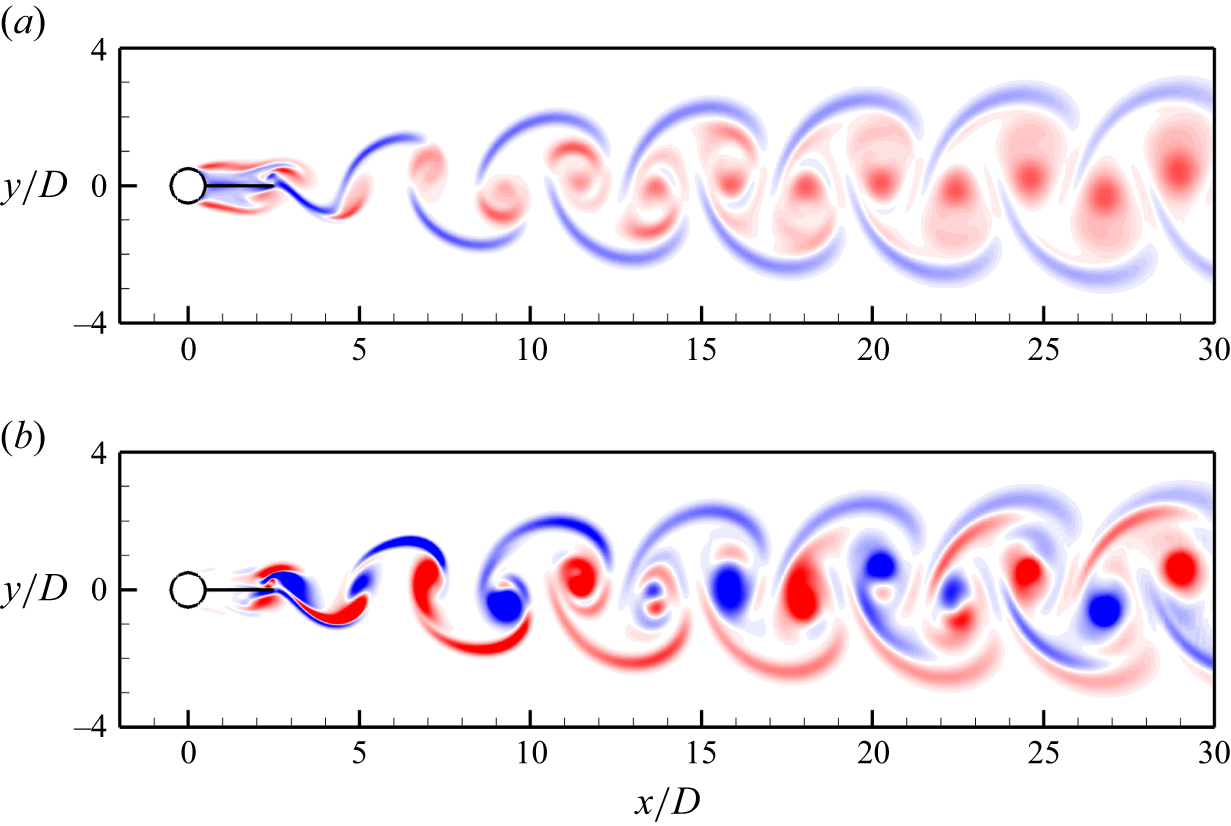
Figure 13. Streamwise perturbation vorticity fields for the case (L/D, Re) = (2, 330): (a) mode BL predicted at $ \beta $
D = 0.4, and (b) mode A predicted at
$ \beta $
D = 0.4, and (b) mode A predicted at $ \beta $
D = 2.0. Red and blue denote positive and negative vorticity values, respectively.
$ \beta $
D = 2.0. Red and blue denote positive and negative vorticity values, respectively.
Figure 14 illustrates the overall wake structures for L/D = 2 predicted by the 3-D DNS with L z /D = 32. For Re slightly above the Re cr3D of 325.5, e.g. at Re = 330, nine spanwise periods of the stable mode A structure are observed at the initial stage of the simulation (figure 14 a). The spanwise wavelength of the stable mode A structure is approximately 3.6D, which is close to the most unstable wavelength predicted by the Floquet analysis (i.e. 3.3D at Re = 330). With the evolution in time, the stable mode A structure decays gradually. The gradual decay of the stable mode A structure over the initial stage is also observed for Re = 320 (<Re cr3D), which indicates that the stable mode A structure is triggered by the initial disturbance prescribed in the domain for the generation of flow three-dimensionality. Since the stable mode A is marginally stable (figure 12 a), it may be triggered by the initial disturbance but cannot persist indefinitely. As shown in figure 14(b), the fully developed wake for Re = 330 is represented by two spanwise periods of ordered mode BL structure, because mode BL is the only unstable mode (figure 12 a). As Re increases to 360, 400 and 440, the mode BL structure becomes increasingly disordered (e.g. figure 14 c), yet the symmetry pattern of mode BL is still visible. With the further increase in Re to 480, the mode BL structure is no longer visible, and the wake is represented by chaotic finer-scale structures (figure 14 d).
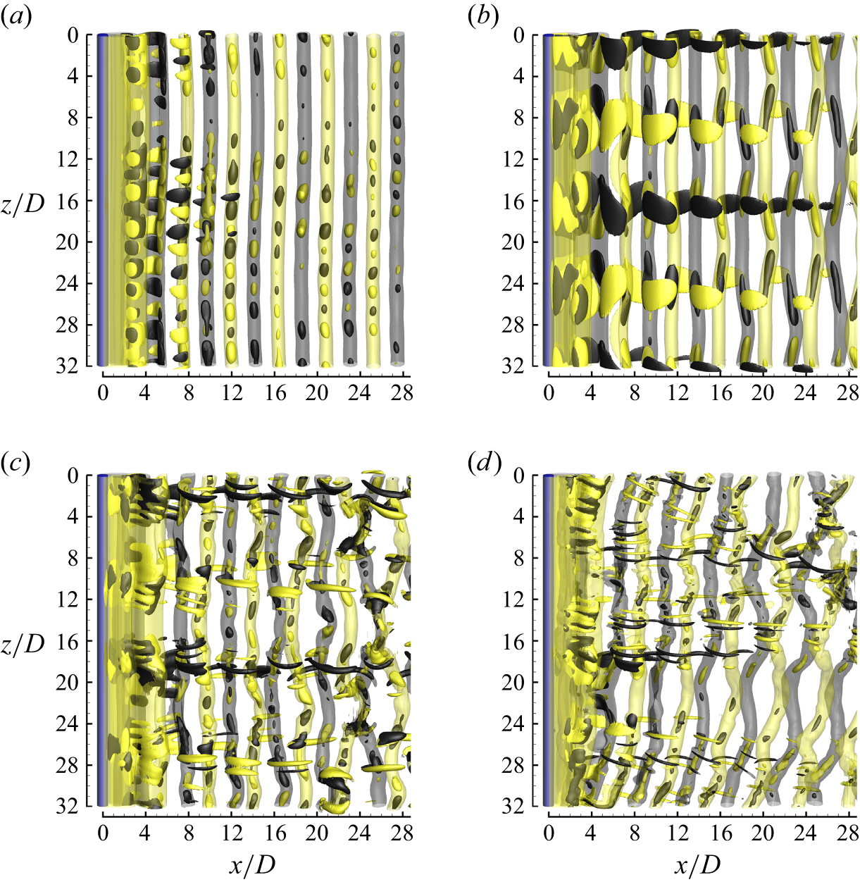
Figure 14. Instantaneous vorticity fields for L/D = 2: (a) Re = 330 (stable mode A structure before evolution to mode BL), (b) Re = 330 (ordered mode BL structure in the fully developed flow), (c) Re = 400 (disordered mode BL structure) and (d) Re = 480 (chaotic fine-scale structures). The translucent iso-surfaces represent spanwise vortices with | $\omega_z$
| = 0.5, while the opaque iso-surfaces represent streamwise vortices with |
$\omega_z$
| = 0.5, while the opaque iso-surfaces represent streamwise vortices with | $\omega_x$
| = 0.08, 0.2, 0.5 and 1.0 for panels (a–d), respectively.
$\omega_x$
| = 0.08, 0.2, 0.5 and 1.0 for panels (a–d), respectively.
4.4. Three-dimensional results for L/D = 4–6
While mode BL dominates the 3-D wake patterns for L/D = 2–3, it becomes a marginally stable mode for L/D = 4 (figure 15
a), and is no longer detected for L/D = 5 and 6 (omitted for brevity). For the mode BL peak observed in figure 15(a), a curve fitting of the peak $| \mu |$
values for Re = 340–400 indicates that the most unstable condition occurs at Re = 368, with the largest
$| \mu |$
values for Re = 340–400 indicates that the most unstable condition occurs at Re = 368, with the largest $| \mu |$
value of 0.97, which confirms that mode BL is now stable. For L/D = 4–6, the only unstable mode up to at least Re = 440 is a QP mode called QP3, and its neutral instability curve is presented in figure 15(b).
$| \mu |$
value of 0.97, which confirms that mode BL is now stable. For L/D = 4–6, the only unstable mode up to at least Re = 440 is a QP mode called QP3, and its neutral instability curve is presented in figure 15(b).
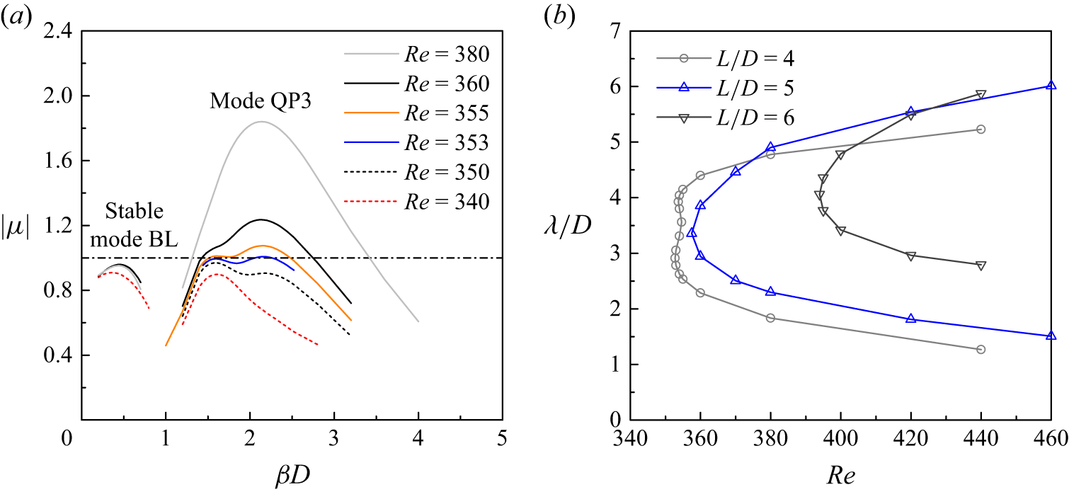
Figure 15. Floquet analysis results for L/D = 4–6: (a) the $| \mu |$
–
$| \mu |$
– $ \beta $
relationships for L/D = 4, and (b) the neutral instability curves for the 3-D wake instability mode, i.e. mode QP3.
$ \beta $
relationships for L/D = 4, and (b) the neutral instability curves for the 3-D wake instability mode, i.e. mode QP3.
Figure 16 shows the 3-D DNS results for L/D = 4, where the 3-D wake pattern is now dominated by mode QP3. For Re slightly above the Re cr3D of 352.8, e.g. at Re = 360, six relatively ordered spanwise periods of the mode QP3 structure are observed in the fully developed flow (figure 16 a). The spanwise wavelength of the mode QP3 structure is approximately 2.7D, which is close to the most unstable wavelength predicted by the Floquet analysis (i.e. 2.9D at Re = 360). With the further increase in Re over 360–480, the mode QP3 structure becomes increasingly disordered (figure 16).
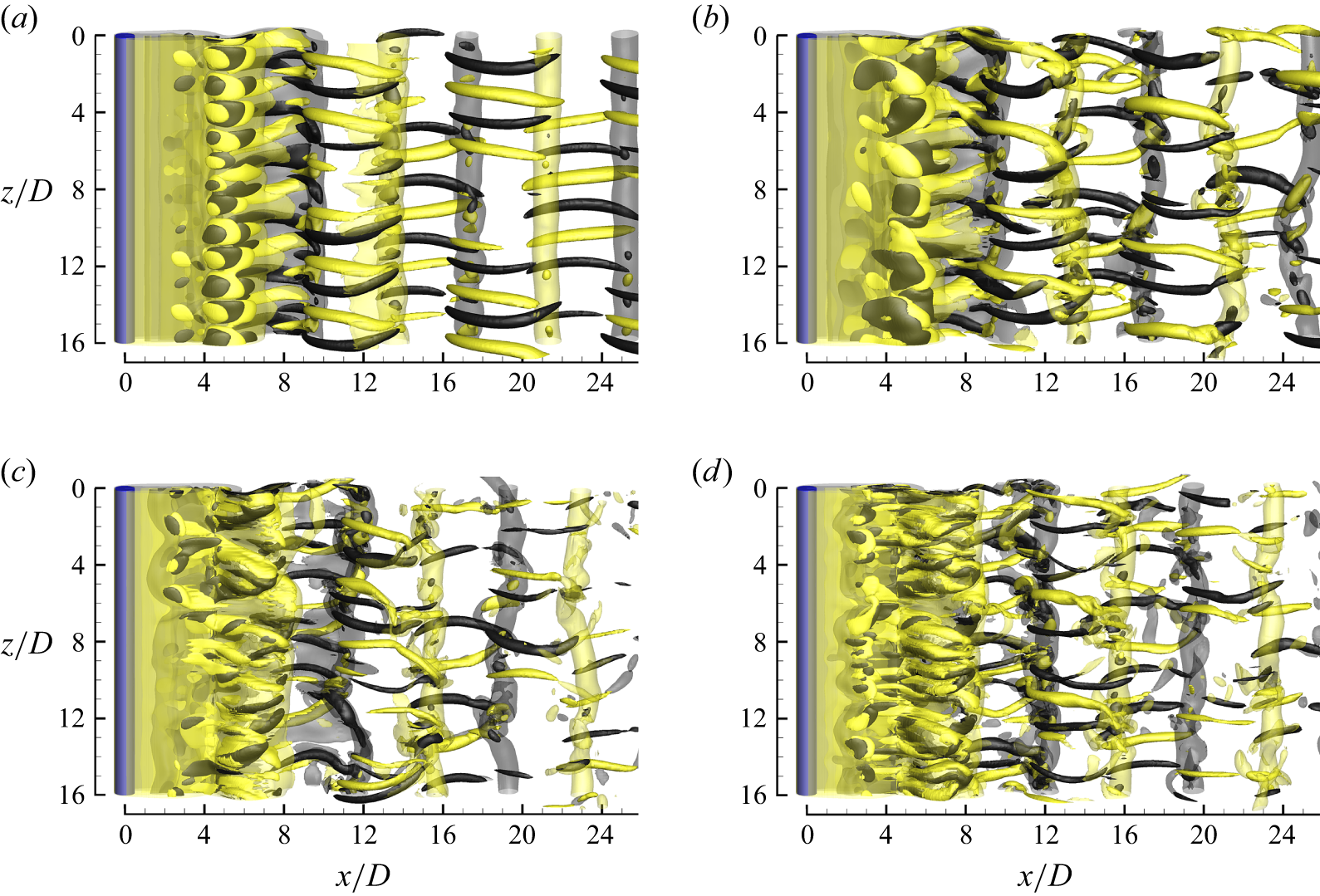
Figure 16. Instantaneous vorticity fields for L/D = 4: (a) Re = 360, (b) Re = 380, (c) Re = 420 and (d) Re = 480. The translucent iso-surfaces represent spanwise vortices with | $\omega_z$
| = 0.5, while the opaque iso-surfaces represent streamwise vortices with |
$\omega_z$
| = 0.5, while the opaque iso-surfaces represent streamwise vortices with | $\omega_x$
| = 0.3, 0.6, 1.0 and 1.0 for panels (a–d), respectively.
$\omega_x$
| = 0.3, 0.6, 1.0 and 1.0 for panels (a–d), respectively.
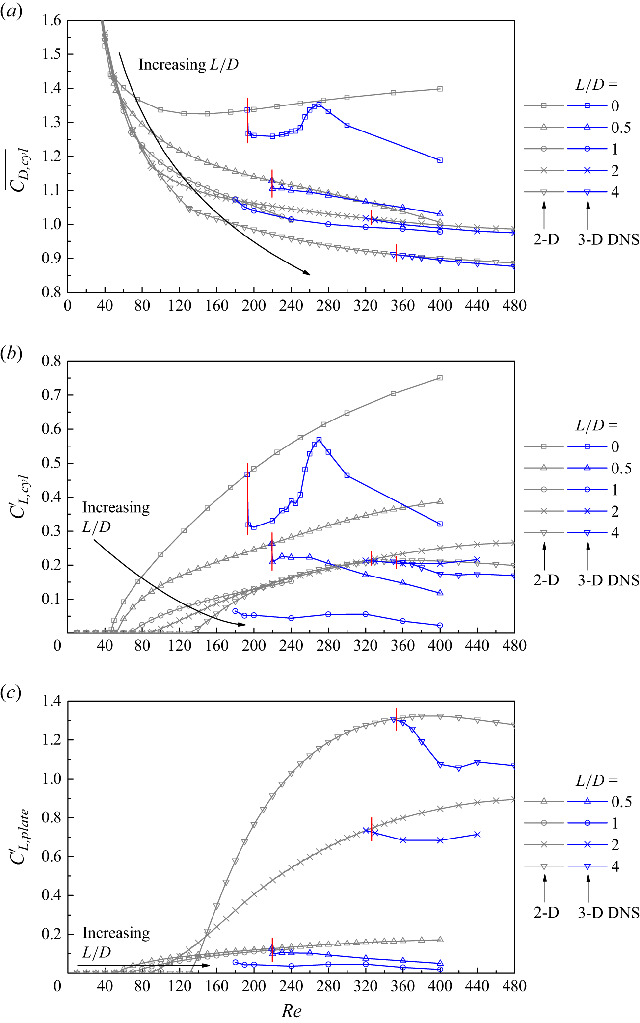
Figure 17. Hydrodynamic coefficients computed by the 2-D and 3-D DNSs, including the (a) $\overline{C_{D,cyl}}-Re$
, (b)
$\overline{C_{D,cyl}}-Re$
, (b) $C'_{L,cyl}-Re$
and (c)
$C'_{L,cyl}-Re$
and (c) $C'_{L,\textit{plate}}-Re$
relationships. For each L/D condition (apart from L/D = 1), the Re
cr3D value is indicated by a red vertical bar.
$C'_{L,\textit{plate}}-Re$
relationships. For each L/D condition (apart from L/D = 1), the Re
cr3D value is indicated by a red vertical bar.
4.5. Summary of the 3-D wake transition process
The Floquet analysis and 3-D DNS results presented in §§ 4.1 to 4.4 reveal significantly different 3-D unstable modes and wake structures for different L/D conditions. Nevertheless, the 3-D wake transition processes for different L/D conditions share some general similarities. Specifically, over a certain range of Re above the Re cr3D value, the real 3-D flow is dominated by the first unstable mode predicted by the Floquet analysis, which is reasonable. With the increase in Re, the spanwise wavelength of the wake structure gradually decreases, and the wake structure becomes increasingly chaotic. This process is realised through either emergence of additional finer-scale unstable modes in the 3-D flow (e.g. L/D = 0.5 and 1), or progressive irregularity and breakdown of the modal structure itself (e.g. L/D ≥ 2). In any case, the wake is dominated by chaotic small-scale structures (with λ/D ≲ 1) at the largest Re simulated in this study, and the wake is expected to become increasingly chaotic and turbulent with further increase in Re.
Over the wake transition process from two to three dimensions and eventually to chaos and turbulence, the monotonic decrease in the spanwise wavelength of the 3-D wake structures with increasing Re appears to be a common phenomenon in various bluff-body flows. Other than the present scenarios, this phenomenon is also observed for the flow around a circular cylinder (Jiang et al. Reference Jiang, Cheng, Draper, An and Tong2016), a square cylinder with various incidence angles (Yoon, Yang & Choi Reference Yoon, Yang and Choi2012; Jiang, Cheng & An Reference Chutkey, Suriyanarayanan and Venkatakrishnan2018; Jiang Reference Duan and Wang2021), a rectangular cylinder with various cross-sectional aspect ratios (Ju & Jiang Reference Ju and Jiang2024), etc. This phenomenon suggests that, with the increase in Re, new unstable Floquet modes with decreasing (rather than increasing) spanwise wavelengths are much more likely to be actually manifested in the real 3-D flow. Eventually, the small-scale 3-D wake structures become increasingly chaotic with increasing Re, which facilitates evolution of turbulence in the wake.
4.6. Variations in the hydrodynamic forces
The effects of flow three-dimensionality on the hydrodynamic forces are reflected by a comparison of the forces computed by the 2-D and 3-D DNSs. Figure 17(a,b) shows the mean drag and fluctuating lift on the cylinder for various L/D conditions. For the cases with a splitter plate (i.e. L/D ≥ 0.5), the mean drag is hardly affected by the flow three-dimensionality, while the fluctuating lift is affected to a greater extent. This is because the fluctuating lift is completely induced by the alternate formation of the low pressure regions in the near wake, such that it is more sensitive to the influence of the flow three-dimensionality on the low pressure regions.
The effects of flow three-dimensionality on the fluctuating lift on the cylinder are examined in detail. As shown in figure 17(b), for L/D = 0.5 and 1, the flow three-dimensionality has a strong effect in reducing the fluctuating lift. In general, this effect increases with increasing Re, because the increasingly finer-scale and chaotic 3-D wake structures result in an increased degree of flow three-dimensionality. For L/D ≥ 2, however, the effect of flow three-dimensionality on the lift reduction becomes rather weak (the lift reduction induced by the flow three-dimensionality is less than 10 % of that induced by the alteration of the 2-D flow by the splitter plate). With the increase in L/D from 1 to 2, the streamwise location for the formation of the primary vortices moves from downstream of the splitter plate to the two sides of the plate. Nevertheless, the 3-D wake structures are destabilised downstream of the plate based on the interaction of the primary vortices of opposite signs (figure 13). Therefore, the low pressure regions, which govern the fluctuating lift on the cylinder, are mainly shaped by the formation of the primary vortices on the two sides of the plate, and are relatively less affected by the flow three-dimensionality developed further downstream (in contrast to L/D ≤ 1 where the primary vortices and the 3-D wake structures are both developed downstream of the plate).
For L/D ≤ 1, in addition to the relatively strong contribution of the 3-D wake structures on the lift reduction, the relatively small Re cr3D values also contribute to an early start (in terms of Re) for the influence of flow three-dimensionality on the lift reduction, such that, when compared at the same Re value, relatively large lift reductions are observed for L/D ≤ 1. For example, after taking into account the 3-D effects, L/D = 0.5 may even outperform L/D = 4 in the lift reduction (and the associated suppression/mitigation of the VIV and acoustic noise).
Figure 17(c) examines the fluctuating lift on the plate. For each 3-D case, the flow three-dimensionality results in almost identical percentage reductions in the fluctuating lift on the cylinder and the plate. A combination of figure 17(b,c) suggests that the use of a plate of L/D = 1 may suppress the fluctuating lift on the cylinder–plate system almost completely.
To reveal this optimal suppression more clearly, figure 18 shows the mean drag and fluctuating lift coefficients computed by the 3-D DNS at a fixed Re of 400. The minimum fluctuating lift is indeed observed at L/D = 1 (figure 18 b). For L/D ∼ 0.5–1.3, the fluctuating lift remains at a relatively small level, and the mean drag also displays a local trough, which suggests good performance of the splitter plate over this range of L/D.
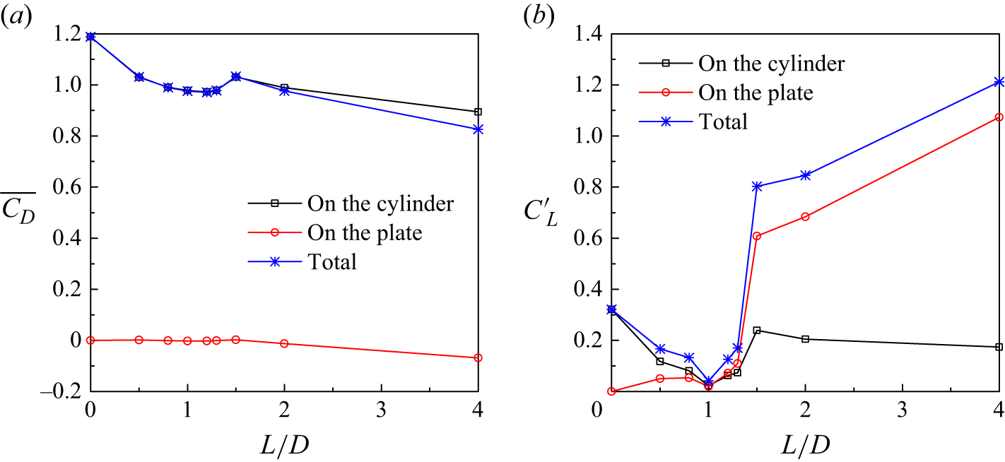
Figure 18. Hydrodynamic coefficients computed by the 3-D DNS at Re = 400: (a) the mean drag coefficient, and (b) the root-mean-square lift coefficient.
4.7. Hysteresis effect at the onset of three-dimensionality
The existence or absence of a hysteresis effect at the onset of three-dimensionality may be identified by several methods, as summarised in table 6. With the availability of the 3-D hydrodynamic forces shown in figure 17, the simplest method (method 1 in table 6) is to identify the sudden or gradual variation in the 3-D forces at Re cr3D. A sudden variation in the forces arises from a sudden increase in the degree of three-dimensionality at Re cr3D due to a specific 3-D wake instability mode, which corresponds to a subcritical instability (hysteretic condition) of the flow (Jiang et al. Reference Chutkey, Suriyanarayanan and Venkatakrishnan2018). In contrast, a gradual variation in the forces at Re cr3D corresponds to a supercritical instability (non-hysteretic condition) of the flow (Jiang et al. Reference Chutkey, Suriyanarayanan and Venkatakrishnan2018). As shown in figure 17, sudden variations in the forces at Re cr3D are observed for L/D = 0 and 0.5, which indicates that the corresponding mode A instability is subcritical (hysteretic). In contrast, gradual variations in the forces at Re cr3D are observed for L/D = 2 and 4, which indicates that the corresponding modes BL and QP3 instabilities, respectively, are both supercritical (non-hysteretic).
Table 6. Hysteresis effect at the onset of three-dimensionality identified by different methods.
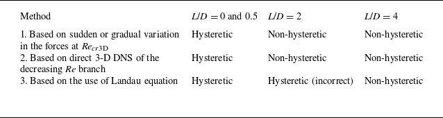
The hysteresis effect can also be confirmed by additional 3-D DNS of the decreasing Re branch (method 2 in table 6), where a fully developed flow field with Re slightly above Re cr3D is employed as the initial condition, and additional DNSs with a stepwise decrease in Re can reveal the critical Re below which the wake transitions back to two-dimensional. To minimise the computational cost for this set of DNSs, the spanwise domain length L z may be set to the most unstable spanwise wavelength of the first 3-D wake instability mode, such that only one spanwise period of the 3-D mode is resolved. For L/D = 0.5, the initial condition for the additional 3-D DNS is a spanwise period of the mode A structure obtained at Re = 220 (> Re cr3D = 219.6), and a stepwise decrease in Re at an interval of 1 reveals the critical Re of 214 for the 3-D-to-2-D transition, which confirms that the mode A instability is hysteretic. In contrast, the initial conditions of a spanwise period of mode BL structure for L/D = 2 at Re = 326 (> Re cr3D = 325.5) and a spanwise period of mode QP3 structure for L/D = 4 at Re = 353.5 (> Re cr3D = 352.8) both decay to two dimensions after a decrease in Re by 1, which confirms that the modes BL and QP3 instabilities are non-hysteretic.
The Landau equation (Landau & Lifshitz Reference Landau and Lifshitz1976) (method 3 in table 6) is also commonly used in the literature for the identification of the hysteresis effect (e.g. Dušek, Le Gal & Fraunié Reference Dušek, Le Gal and Fraunié1994; Henderson & Barkley Reference Williamson1996; Thompson, Leweke & Provansal Reference Posdziech and Grundmann2001; Sheard, Thompson & Hourigan Reference Sheard, Thompson and Hourigan2004; Carmo et al. Reference Carmo, Sherwin, Bearman and Willden2008). For the amplitude A(t) of a 3-D perturbation mode, the Landau equation can be written up to third order as
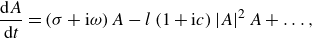 \begin{align} \frac{\mathrm{d}A}{\mathrm{d}t}=\left(\sigma +\mathrm{i}\omega \right)A-l\left(1+\mathrm{i}c\right)\left| A\right| ^{2}A+\ldots , \end{align}
where σ is the linear growth rate of the perturbation, $\omega$
is the angular oscillation frequency during the linear growth phase and c is the Landau constant. The l-coefficient is determined by plotting d(log|A|)/dt against |A|2, where the slope of the curve near |A|2 = 0 gives –l. The hysteresis of the wake instability mode is determined based on the sign of the l-coefficient, where a positive l corresponds to a non-hysteretic flow, while a negative l corresponds to a hysteretic flow. More details on this method can be found in Dušek et al. (Reference Dušek, Le Gal and Fraunié1994), Sheard et al. (Reference Sheard, Thompson and Hourigan2004) and Carmo et al. (Reference Carmo, Sherwin, Bearman and Willden2008).
$\omega$
is the angular oscillation frequency during the linear growth phase and c is the Landau constant. The l-coefficient is determined by plotting d(log|A|)/dt against |A|2, where the slope of the curve near |A|2 = 0 gives –l. The hysteresis of the wake instability mode is determined based on the sign of the l-coefficient, where a positive l corresponds to a non-hysteretic flow, while a negative l corresponds to a hysteretic flow. More details on this method can be found in Dušek et al. (Reference Dušek, Le Gal and Fraunié1994), Sheard et al. (Reference Sheard, Thompson and Hourigan2004) and Carmo et al. (Reference Carmo, Sherwin, Bearman and Willden2008).
In the present study, the Landau equation is applied to the cases with Re slightly above Re cr3D and L z close to the most unstable spanwise wavelength of the first 3-D wake instability mode, i.e. (L/D, Re, L z ) = (0.5, 220, 4) for mode A, (2, 327, 13.67) for mode BL and (4, 355, 2.91) for mode QP3. Figure 19(a–c) shows the time evolution of the mode amplitude |A|, which is measured from the envelope of the fluctuation of the spanwise velocity sampled at (x/D, y/D) = (5, 1) and a z/D within the 3-D mode structure. Based on the corresponding l-coefficient determined from figure 19(d–f), the cases with L/D = 0.5, 2 and 4 are deemed hysteretic, hysteretic and non-hysteretic, respectively.
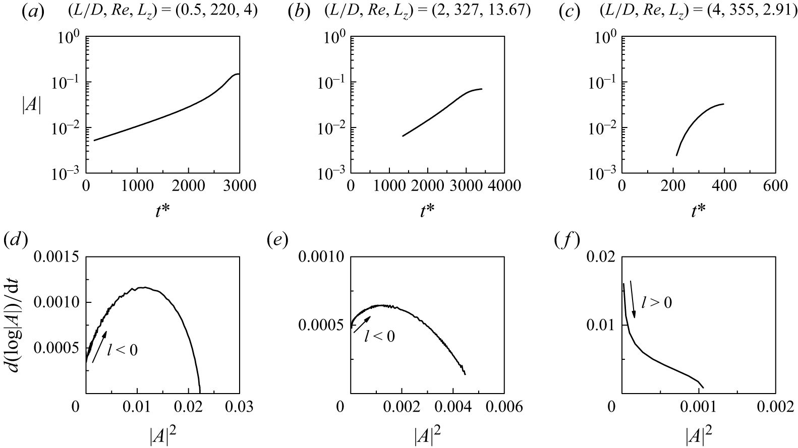
Figure 19. Identification of the hysteresis effect using the Landau equation: (a) time evolution of the mode amplitude |A| for the case (L/D, Re, L z ) = (0.5, 220, 4), (b) time evolution of |A| for the case (L/D, Re, L z ) = (2, 327, 13.67), (c) time evolution of |A| for the case (L/D, Re, L z ) = (4, 355, 2.91) and (d–f) the [d(log|A|)/dt] –|A|2 relationships for the corresponding cases shown in panels (a–c), respectively.
As summarised in table 6, the three methods lead to consistent conclusions for the cases with L/D = 0, 0.5 and 4, but discrepancies for the case with L/D = 2. We believe that the error lies in the use of the Landau equation for the case with (L/D, Re, L z ) = (2, 327, 13.67). For this case, the flow is initialised with several spanwise periods of the marginally stable mode A (figure 12 a) structure, followed by the dominance of a spanwise period of the unstable mode BL (figure 12 a) structure at t * ≳ 1000 (similar to the flow evolution shown in figure 14 a,b). Although the Landau equation is applied to the time range of t * ≳ 1350 (figure 19 b), which corresponds to the dominance of the unstable mode BL only, the time evolution of |A| may still be contaminated by the initial development of the stable mode A and lead to a false conclusion on the existence of hysteresis. In comparison, methods 1 and 2 are based on the fully developed flow only, and are thus unaffected by the initial transients.
5. Conclusions
This paper investigates the 2-D and 3-D wake transitions, 3-D wake instability modes, 3-D wake structures and 2-D and 3-D hydrodynamic characteristics for a circular cylinder with a rear-attached splitter plate, over a parameter space of Re = 10–480 and L/D = 0–6.
With the increase in L/D, the Re cr2D value increases monotonically. This is because when the vortex shedding is forced to occur further downstream by the increase in L/D, the separating shear layers at the location of vortex shedding are further weakened by (i) the elongation of the separating shear layers, and (ii) the shear layers developed on the two sides of the no-slip plate. Therefore, an increased Re is required for the separating shear layers to gain more strength to roll up into vortices.
The Re cr3D value and the 3-D unstable modes and structures are also significantly altered by the splitter plate. Compared with Re cr3D = 189.8 for an isolated cylinder, the onset of three-dimensionality is brought forward to Re cr3D < 100 for L/D = 1 and significantly delayed to Re cr3D > 320 for L/D = 2–6. With the increase in L/D, the first 3-D unstable mode/structure changes in the sequence of (i) mode A for L/D = 0–0.5, (ii) mode AL for L/D = 1, (iii) mode BL for L/D = 2–3 and (iv) mode QP3 for L/D = 4–6. For each L/D category, the 3-D wake transition process and mode interactions are revealed by the DNSs. A general similarity is that the spanwise wavelength of the 3-D wake structures decreases monotonically with increasing Re, which is realised through either emergence of additional finer-scale unstable modes in the 3-D flow (e.g. L/D = 0.5 and 1), or progressive irregularity and breakdown of the modal structure itself (e.g. L/D ≥ 2). Eventually, the small-scale 3-D wake structures become increasingly chaotic with increasing Re, which facilitates evolution of turbulence in the wake.
The strong influence of the splitter plate on the formation of the primary vortices and 3-D wake structures alter the hydrodynamic characteristics strongly. In particular, optimal lift reduction is achieved at L/D ∼ 1 (rather than at very large L/D), and its physical reason is explained based on the spanwise and streamwise wake structures and the Re cr3D values examined in this study.
At the onset of three-dimensionality, a hysteresis effect is identified for the mode A instability for L/D = 0 and 0.5, but not for the modes BL and QP3 instabilities for L/D = 2 and 4, respectively. In addition, we discussed strength and limitation of the three methods for the identification of the hysteresis effect (based on (i) sudden or gradual variation in the forces at Re cr3D, (ii) direct 3-D DNS of the decreasing Re branch and (iii) the use of Landau equation). The first two methods draw conclusion from the fully developed flow only, whereas the third method may be contaminated by initial transients induced by stable Floquet modes and may thus lead to a false conclusion on the existence/absence of hysteresis.
Funding
H.J. would like to acknowledge support from National Natural Science Foundation of China (Grant No. 52301341).
Declaration of interests
The author reports no conflict of interest.
Appendix A. Method for the determination of Re cr2D
For each L/D condition, the Re cr2D is determined by the following three steps: (i) computing the cases near the Re cr2D at an interval of ΔRe = 1, (ii) calculating the exponential growth/decay rate of the amplitude of C L for the two cases immediately before and after the instability and (iii) determining the Re cr2D at neutral instability (i.e. zero growth/decay rate) through linear interpolation of the growth/decay rates.
For example, figure 20 shows time histories of C L for L/D = 0.5 and Re = 52 and 53, where the amplitude of C L displays exponential decay and exponential growth, respectively. This feature suggests that Re cr2D is within Re = 52–53. To determine the precise value of Re cr2D, the growth/decay rate of the amplitude of C L is quantified. Specifically, the upper and lower envelopes of the time history of C L are each fitted with an exponential function
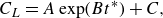 \begin{align} C_{L}=A\exp (Bt^{*})+C ,\end{align}
where A, B and C are curve fitting coefficients. After discarding the initial transients of $t^{*}$
< 100, the coefficient of determination (denoted R2) for the fitted curves is 1.0000, which suggests perfect exponential fitting. Based on the growth/decay rates B obtained at Re = 52 and 53, figure 21 shows a linear fit of the B–Re relationship. The precise value of Re
cr2D (= 52.67) can be determined at the zero growth/decay rate (B = 0).
$t^{*}$
< 100, the coefficient of determination (denoted R2) for the fitted curves is 1.0000, which suggests perfect exponential fitting. Based on the growth/decay rates B obtained at Re = 52 and 53, figure 21 shows a linear fit of the B–Re relationship. The precise value of Re
cr2D (= 52.67) can be determined at the zero growth/decay rate (B = 0).
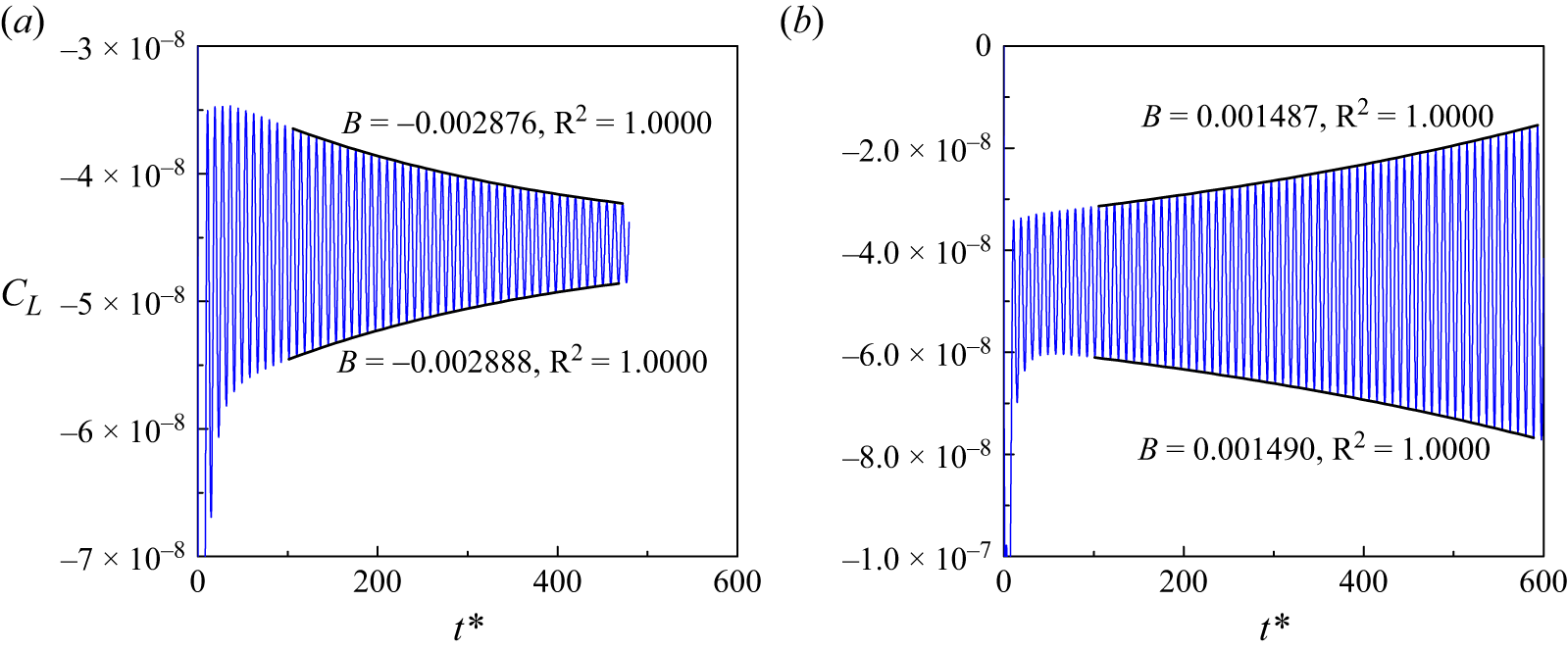
Figure 20. Time history of C L for L/D = 0.5 and (a) Re = 52, and (b) Re = 53. The black curves show exponential fitting of the upper and lower envelopes.
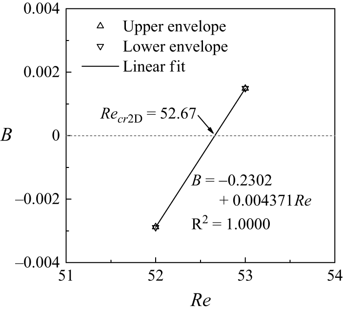
Figure 21. Relationship between the growth/decay rate and the Reynolds number.
It is worth noting that at Re close to Re
cr2D, the fully developed flow with vortex shedding may be established after time evolution of a long period (with $t^{*}$
> 104), which requires a significant computational cost. The merit of the present method is that it does not require vortex shedding to be visualised. The precise Re
cr2D value can be determined at t
* well within 103.
$t^{*}$
> 104), which requires a significant computational cost. The merit of the present method is that it does not require vortex shedding to be visualised. The precise Re
cr2D value can be determined at t
* well within 103.


 Open access