


1. Introduction
Pilot-wave hydrodynamics (Bush Reference Bush2015) was initiated by the discovery of Yves Couder and Emmanuel Fort that millimetric droplets may self-propel or ‘walk’ across the surface of a vibrating liquid bath, propelled by their own wave field (Couder et al. Reference Couder, Protière, Fort and Boudaoud2005). This walking-droplet system has provided the basis for the nascent field of hydrodynamic quantum analogues, which is devoted to exploring the ability of this system to capture features typically associated with the quantum realm (Bush & Oza Reference Bush and Oza2020). The key feature responsible for the emergent quantum-like behaviour is the non-Markovian nature of the droplet dynamics: the bath serves as the memory of the droplet, the extent of which depends on the longevity of the Faraday pilot-wave field as is prescribed by the vibrational acceleration’s proximity to the Faraday threshold (Eddi et al. Reference Eddi, Sultan, Moukhtar, Fort, Rossi and Couder2011). When the walkers are confined by applied forces, the droplets may execute circular orbits (see figure 1), arising through the balance of the inward confining force and the outward inertial force. At high memory, the circular orbits become quantised owing to the dynamical constraint imposed on the droplet by its pilot wave, which serves as an effective self-potential (Fort et al. Reference Fort, Eddi, Moukhtar, Boudaoud and Couder2010; Oza et al. Reference Oza, Harris, Rosales and Bush2014a ). We here present the results of a theoretical investigation in which we compare the onset of orbital instability and quantisation for pilot-wave hydrodynamics in the presence of a radial force field and in a rotating frame. Doing so allows us to assess the relative importance of the imposed potential and the memory-induced self-potential on the orbital stability.
Fort et al. (Reference Fort, Eddi, Moukhtar, Boudaoud and Couder2010) examined droplets walking in a rotating frame, so subjected to a Coriolis force. At low memory, the droplet executes anticyclonic inertial orbits at its free-walking speed, in which the outward inertial force is balanced by the confining Coriolis force. The orbital radius reflects this balance and differs from that of classical inertial orbits only through the wave-induced added mass of the droplet (Bush, Oza & Moláček Reference Bush, Oza and Moláček2014; Oza et al. Reference Oza, Harris, Rosales and Bush2014a ). At higher memory, the droplet encounters its own wake, which comprises a circular corrugation on the free surface, centred on the orbital centre (see figure 1 b). As a consequence, the droplet is restricted to one of a set of circular orbits with quantised radii corresponding approximately to integer multiples of half the Faraday wavelength (Fort et al. Reference Fort, Eddi, Moukhtar, Boudaoud and Couder2010; Blitstein, Rosales & Sáenz Reference Blitstein, Rosales and Sáenz2024). This radial quantisation may be rationalised in terms of the successive destabilisation of orbits of other radii as the path memory is increased (Fort et al. Reference Fort, Eddi, Moukhtar, Boudaoud and Couder2010; Harris & Bush Reference Harris and Bush2014; Oza et al. Reference Oza, Harris, Rosales and Bush2014a ). As the orbital radius is increased progressively, the instabilities are marked by either monotonically growing perturbations or resonant wobbles with a wobbling frequency twice the orbital frequency (Oza et al. Reference Oza, Harris, Rosales and Bush2014a ; Liu, Durey & Bush Reference Liu, Durey and Bush2023), as depicted in figure 2(a,b). At the highest memory considered, Harris & Bush (Reference Harris and Bush2014) demonstrated that these quantised orbits destabilise into chaotic trajectories marked by intermittent switching between quantised orbits, a feature captured in accompanying theoretical (Oza et al. Reference Oza, Harris, Rosales and Bush2014a ) and numerical (Oza et al. Reference Oza, Wind-Willassen, Harris, Rosales and Bush2014b ) investigations.
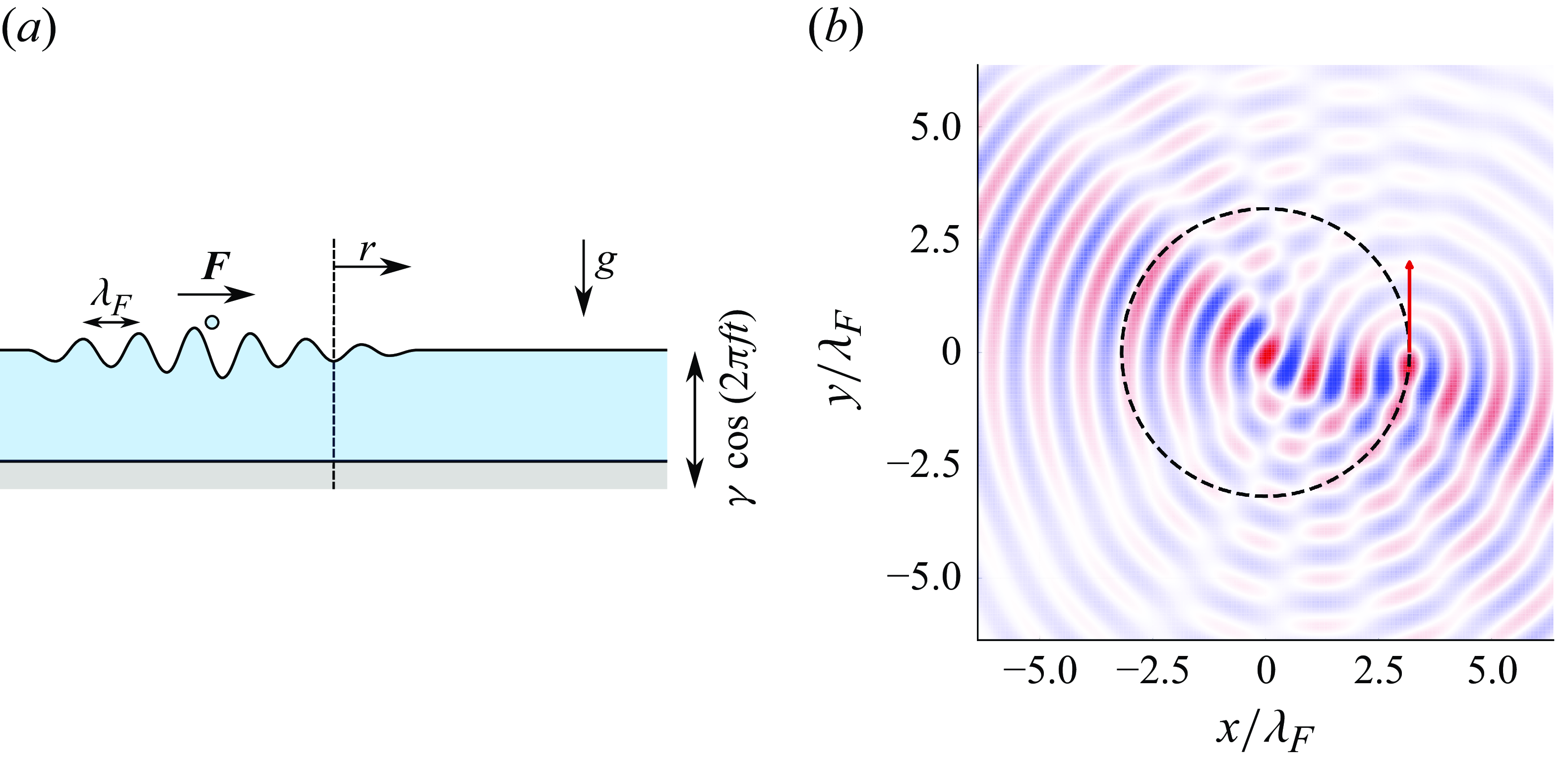
Figure 1. Orbital pilot-wave dynamics in a confining force field. (a) Schematic diagram of the physical system, in which a droplet walks along a liquid bath driven vertically with acceleration $\gamma \cos (2\pi ft)$
. Two distinct force fields are considered. In the first, the system rotates at an angular velocity
$\gamma \cos (2\pi ft)$
. Two distinct force fields are considered. In the first, the system rotates at an angular velocity $\boldsymbol{\Omega } = \Omega \boldsymbol{\hat {z}}$
, so the droplet is subjected to a Coriolis force and is thus prone to anticyclonic circular orbits. In the second, the droplet is constrained by a central force
$\boldsymbol{\Omega } = \Omega \boldsymbol{\hat {z}}$
, so the droplet is subjected to a Coriolis force and is thus prone to anticyclonic circular orbits. In the second, the droplet is constrained by a central force $\boldsymbol{F} = -\boldsymbol \nabla V\!(r)$
. The vertical axis represents either the centre of force for a central force, or the rotation axis,
$\boldsymbol{F} = -\boldsymbol \nabla V\!(r)$
. The vertical axis represents either the centre of force for a central force, or the rotation axis, $\boldsymbol{\hat {z}}$
, in the rotating system. (b) Simulated wave field generated by a droplet walking in a circular orbit (black dashed circle) at high memory. Red and blue designate regions of elevation and depression, and white indicates no surface displacement. The Faraday wavelength is
$\boldsymbol{\hat {z}}$
, in the rotating system. (b) Simulated wave field generated by a droplet walking in a circular orbit (black dashed circle) at high memory. Red and blue designate regions of elevation and depression, and white indicates no surface displacement. The Faraday wavelength is $\lambda _F = 4.75\,\textrm{mm}$
for the experimental parameters detailed in § 3.
$\lambda _F = 4.75\,\textrm{mm}$
for the experimental parameters detailed in § 3.
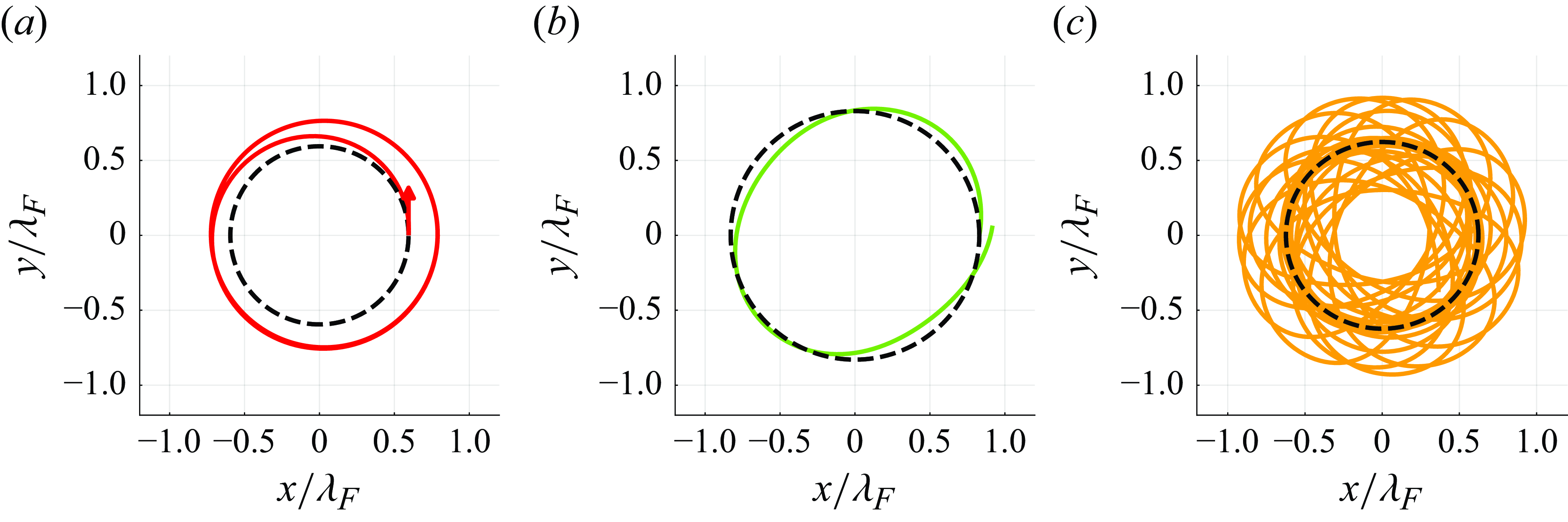
Figure 2. Three forms of orbital instability. Evolution of the droplet trajectory when perturbed from an unstable circular orbit (dashed curve), with (a) a monotonic instability, (b) a $2\omega$
instability and (c) a
$2\omega$
instability and (c) a $\sqrt {2}\omega$
instability, where
$\sqrt {2}\omega$
instability, where $\omega$
is the orbital frequency. Monotonic instabilities lead to a jump up/down to a nearby stable circular orbit,
$\omega$
is the orbital frequency. Monotonic instabilities lead to a jump up/down to a nearby stable circular orbit, $2\omega$
-instabilities lead to a stable 2-wobble orbit and
$2\omega$
-instabilities lead to a stable 2-wobble orbit and $\sqrt {2}\omega$
-instabilities lead to quasi-periodic wobbling, for which the wobbling frequency is incommensurate with the orbital frequency. Monotonic and
$\sqrt {2}\omega$
-instabilities lead to quasi-periodic wobbling, for which the wobbling frequency is incommensurate with the orbital frequency. Monotonic and $2\omega$
-instabilities are prevalent for orbital motion in a rotating frame, whereas
$2\omega$
-instabilities are prevalent for orbital motion in a rotating frame, whereas $2\omega$
- and
$2\omega$
- and $\sqrt {2}\omega$
-wobbles mark the onset of instability in the presence of a linear spring force.
$\sqrt {2}\omega$
-wobbles mark the onset of instability in the presence of a linear spring force.
Quantised orbital motion may also be induced when the droplet is confined by a central force. This configuration was first explored experimentally by Perrard et al. (Reference Perrard, Labousse, Fort and Couder2014a
,Reference Perrard, Labousse, Miskin, Fort and Couder
b
), who applied a vertical magnetic field with a radial gradient to a droplet filled with ferrofluid, thereby imparting a linear spring force to the droplet. The authors discovered that the droplet has a propensity for orbits that are quantised in both mean radial position and mean angular momentum, which include circles, lemniscates and trefoils (Labousse et al. Reference Labousse, Perrard, Couder and Fort2014). While the radii of the circular orbits were found to be quantised in a fashion similar to those arising in a rotating frame (Labousse et al. Reference Labousse, Oza, Perrard and Bush2016; Durey & Milewski Reference Durey and Milewski2017), different instabilities set in as the memory was increased. Specifically, all instabilities were found to be wobbles (Tambasco et al. Reference Tambasco, Harris, Oza, Rosales and Bush2016), with the wobbling frequency being either close to $2\omega$
(see figure 2
b), and thus resonant with the orbital frequency,
$2\omega$
(see figure 2
b), and thus resonant with the orbital frequency, $\omega$
, or close to
$\omega$
, or close to $\sqrt {2}\omega$
(see figure 2
c), and thus non-resonant (Labousse & Perrard Reference Labousse and Perrard2014). As arose in the rotating frame, at higher memory, the periodic orbital states destabilise, leading to an intermittent switching between unstable periodic orbits (Perrard et al. Reference Perrard, Labousse, Fort and Couder2014a
,Reference Perrard, Labousse, Miskin, Fort and Couder
b
).
$\sqrt {2}\omega$
(see figure 2
c), and thus non-resonant (Labousse & Perrard Reference Labousse and Perrard2014). As arose in the rotating frame, at higher memory, the periodic orbital states destabilise, leading to an intermittent switching between unstable periodic orbits (Perrard et al. Reference Perrard, Labousse, Fort and Couder2014a
,Reference Perrard, Labousse, Miskin, Fort and Couder
b
).
A similar progression from periodic orbits to chaotic trajectories was reported by Cristea-Platon, Sáenz & Bush (Reference Cristea-Platon, Sáenz and Bush2018) in their study of walkers confined to circular corrals. Specifically, as the memory was increased progressively, periodic orbital states, such as circles, lemniscates and trefoils, gave way to chaotic motion marked by intermittent switching between these orbits, a progression also captured in the simulations of Durey, Milewski & Wang (Reference Durey, Milewski and Wang2020a
). The effective radial force imparted to the droplet by the submerged topography has been likened to that of a potential that is flat within the corral and increases steeply over the submerged step (Hélias & Labousse Reference Hélias and Labousse2023), as might be modelled by a power-law radial potential (Cristea-Platon et al. Reference Cristea-Platon, Sáenz and Bush2018). Circular orbits have also been observed for walkers over inverted conical topography, for which an effective radial confining potential of the form $V\!(r) \propto r$
was inferred for circular orbits (Turton Reference Turton2020). Orbiting in response to other confining potentials, including a logarithmic (two-dimensional Coulomb) potential (Tambasco et al. Reference Tambasco, Harris, Oza, Rosales and Bush2016) and an oscillatory potential of Bessel form (Tambasco & Bush Reference Tambasco and Bush2018), have been explored numerically. Thus, while walker motion in response to Coriolis and linear central forces will be the focus of our study, we will extend our analysis to consider more general radial forces of interest in pilot-wave hydrodynamics.
$V\!(r) \propto r$
was inferred for circular orbits (Turton Reference Turton2020). Orbiting in response to other confining potentials, including a logarithmic (two-dimensional Coulomb) potential (Tambasco et al. Reference Tambasco, Harris, Oza, Rosales and Bush2016) and an oscillatory potential of Bessel form (Tambasco & Bush Reference Tambasco and Bush2018), have been explored numerically. Thus, while walker motion in response to Coriolis and linear central forces will be the focus of our study, we will extend our analysis to consider more general radial forces of interest in pilot-wave hydrodynamics.
Owing to the complexity of orbital pilot-wave dynamics and the associated linear stability analysis, several heuristic arguments have been proposed in an attempt to predict the critical radii of instability. For a linear central force, Labousse et al. (Reference Labousse, Oza, Perrard and Bush2016) noted that the critical radii correspond approximately to zeros of Bessel functions, which was rationalised in terms of the resonance between the perturbation and the system’s wave modes. Durey (Reference Durey2018) noted that the orbits with the largest wave energy destabilise at the lowest memory and do so with monotonically growing perturbations. The efficacy of both these heuristic arguments was tested by Liu et al. (Reference Liu, Durey and Bush2023) for orbiting in response to a Coriolis force: although a favourable agreement in the critical radii was obtained, neither heuristic argument accounted for the dependence of the critical radii on droplet inertia. For orbiting in a rotating frame, Liu et al. (Reference Liu, Durey and Bush2023) suggested that one can predict the form of orbital instability of a circular orbit of a given radius according to the form of the local mean pilot wave, which acts as a self-potential at high memory. Specifically, monotonic instabilities were found to arise for orbits where the local mean wave force increases with orbital radius, with wobbling instabilities appearing otherwise. We note, however, that all three heuristic arguments are based solely on the structure of the wave field and so cannot predict either the critical memory or the frequency of instability as they do not take into account the form of the external force field.
We here present a theoretical study of the stability of circular orbits for walkers confined by a radial or Coriolis force, the two systems that have been considered experimentally. When the orbits are unstable, three possibilities exist: monotonically growing perturbations, or wobbling at a frequency that is either resonant or non-resonant with the orbital frequency, as detailed in figure 2. We demonstrate that the frequency of instability depends on the relative influence of the wave-induced self-potential and the applied potential. Wave-driven wobbling, which is peculiar to pilot-wave systems, is always resonant. Potential-driven wobbling, which we show to be a generic feature of classical particle motion at constant speed, may be resonant or non-resonant, depending on the precise form of the confining potential.
In § 2, as a point of comparison for the hydrodynamic pilot-wave system, we consider classical orbital mechanics (specifically, constrained particle motion in the absence of a pilot wave) at constant speed. Doing so reveals the frequency of potential-driven wobbling, but does not yield insight into the influence of memory, specifically the geometric constraint imposed by the pilot-wave field, on orbital stability. This dependence is investigated in § 3 by applying linear stability analysis to the stroboscopic pilot-wave model (Oza, Rosales & Bush Reference Oza, Rosales and Bush2013) and so constructing numerically the system’s orbital stability diagram. We highlight the differences between orbital stability in the Coriolis and linear central force systems as the orbital radius and memory are varied, and classify the emergence of wave- and potential-driven instabilities. In § 4, we use asymptotic analysis to deduce the dependence of the critical memory and frequency of instability on the orbital radius for both wave-driven and potential-driven instabilities. We then generalise our analysis to consider the stability of orbits in a variety of confining potentials considered in prior studies of pilot-wave hydrodynamics. Particular attention is given to power-law radial force fields, as may play a role analogous to topographic confinement in, for example, the corral experiments (Harris et al. Reference Harris, Moukhtar, Fort, Couder and Bush2013; Cristea-Platon et al. Reference Cristea-Platon, Sáenz and Bush2018). In § 5, we discuss the emerging physical picture for orbital stability in pilot-wave hydrodynamics along with potential directions for future research.
2. Physical picture
We first consider the behaviour of particles executing circular orbits in the plane in the presence of an axisymmetric potential. Celestial mechanics, wherein satellites or planets may execute circular orbits under the influence of the gravitational force, provides a valuable point of comparison for our study. In such classical orbital dynamics (in which there is no pilot wave), the form of the applied external potential affects the stability of circular orbits. Specifically, it is well established that stable circular orbits in the plane can only be supported for confining potentials of the form $V\!(r) \propto r^q$
provided
$V\!(r) \propto r^q$
provided $q \gt -2$
(Goldstein, Poole & Safko Reference Goldstein, Poole and Safko2002). We begin by re-deriving this result in § 2.1, and then compare it to the analogous stability condition relevant to the hydrodynamic pilot-wave system in § 2.2.
$q \gt -2$
(Goldstein, Poole & Safko Reference Goldstein, Poole and Safko2002). We begin by re-deriving this result in § 2.1, and then compare it to the analogous stability condition relevant to the hydrodynamic pilot-wave system in § 2.2.
2.1. Classical orbital mechanics
We consider the dynamics of a particle of mass $m$
moving in response to an axisymmetric potential,
$m$
moving in response to an axisymmetric potential, $V\!(r)$
, in two dimensions. By denoting the particle position in polar coordinates as
$V\!(r)$
, in two dimensions. By denoting the particle position in polar coordinates as $\boldsymbol{x\!}_p(t) = r(t)(\cos \theta (t),\sin \theta (t))$
, one may express the radial force balance as
$\boldsymbol{x\!}_p(t) = r(t)(\cos \theta (t),\sin \theta (t))$
, one may express the radial force balance as
 \begin{equation} m(\ddot {r} - r\dot {\theta }^2) = -V'(r). \end{equation}
Conservation of angular momentum implies that $l = mr^2\dot {\theta }$
is constant for all time. By substituting
$l = mr^2\dot {\theta }$
is constant for all time. By substituting $\dot {\theta } = l/mr^2$
into (2.1), we deduce that the radial motion of the particle satisfies
$\dot {\theta } = l/mr^2$
into (2.1), we deduce that the radial motion of the particle satisfies
 \begin{gather} m\ddot {r} = -V_{{\textit{eff}}}'(r), \quad \mbox{where}\quad V_{{\textit{eff}}}(r) = V\!(r) + \frac {l^2}{2mr^2} \end{gather}
is the effective potential. Notably, the effective potential is the sum of the applied potential and the so-called centrifugal barrier, which is a potential barrier arising due to the conservation of angular momentum that prevents the particle from approaching the origin.
For steady orbital motion with radius $r_0$
, the radial force balance implies that
$r_0$
, the radial force balance implies that $l^2 = m r_0^3 V'(r_0)$
, which can be satisfied only when
$l^2 = m r_0^3 V'(r_0)$
, which can be satisfied only when $V'(r_0) \gt 0$
. If
$V'(r_0) \gt 0$
. If $r(t) = r_0 + \epsilon r_1(t)$
, the radial perturbation will necessarily evolve according the linearised equation
$r(t) = r_0 + \epsilon r_1(t)$
, the radial perturbation will necessarily evolve according the linearised equation $\ddot {r}_1 + \omega _c^2 r_1 = 0$
, where
$\ddot {r}_1 + \omega _c^2 r_1 = 0$
, where
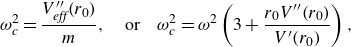 \begin{gather} \omega _c^2 = \frac {V_{{\textit{eff}}}''(r_0)}{m}, \quad \mbox{or}\quad \omega _c^2 = \omega ^2\left (3 + \frac {r_0 V''(r_0)}{V'(r_0)}\right ), \end{gather}
and $\omega = l/mr_0^2$
is the orbital frequency. For a power-law potential of the form
$\omega = l/mr_0^2$
is the orbital frequency. For a power-law potential of the form $V\!(r) \propto r^q$
, we deduce from (2.3) the relationship
$V\!(r) \propto r^q$
, we deduce from (2.3) the relationship $\omega _c^2 = (q+2)\omega ^2$
, which may be used to assess the linear stability of circular orbits. If
$\omega _c^2 = (q+2)\omega ^2$
, which may be used to assess the linear stability of circular orbits. If $q \leqslant -2$
, perturbations grow in time, with circular orbits thus being unstable. Circular orbits thus destabilise if the confining force decays too quickly. Conversely, circular orbits are stable for
$q \leqslant -2$
, perturbations grow in time, with circular orbits thus being unstable. Circular orbits thus destabilise if the confining force decays too quickly. Conversely, circular orbits are stable for $q \gt -2$
, with radial perturbations undergoing closed orbits in phase space. Notably, the perturbation frequency,
$q \gt -2$
, with radial perturbations undergoing closed orbits in phase space. Notably, the perturbation frequency, $\omega _c$
, is generally incommensurate with the orbital frequency,
$\omega _c$
, is generally incommensurate with the orbital frequency, $\omega$
, except when
$\omega$
, except when $q + 2$
is a perfect square.
$q + 2$
is a perfect square.
2.2. Orbital mechanics at a constant speed
A key feature of orbital pilot-wave dynamics in a rotating frame is that the walker speed remains close to the free-walking speed, $u_0$
. While substantial speed variations arise for walker motion in a central force (Perrard et al. Reference Perrard, Labousse, Miskin, Fort and Couder2014b
; Kurianski, Oza & Bush Reference Kurianski, Oza and Bush2017), one expects such variations to be small for nearly circular orbits. To gain insight into the influence of a fixed speed on the stability of circular orbits, we consider the planar motion of a particle of mass
$u_0$
. While substantial speed variations arise for walker motion in a central force (Perrard et al. Reference Perrard, Labousse, Miskin, Fort and Couder2014b
; Kurianski, Oza & Bush Reference Kurianski, Oza and Bush2017), one expects such variations to be small for nearly circular orbits. To gain insight into the influence of a fixed speed on the stability of circular orbits, we consider the planar motion of a particle of mass $m$
moving in response to a potential,
$m$
moving in response to a potential, $V$
, with the particle speed fixed at
$V$
, with the particle speed fixed at $u_0$
for all time. The radial motion of the particle is thus governed by (2.1), whereas the constancy of the particle speed gives rise to the condition
$u_0$
for all time. The radial motion of the particle is thus governed by (2.1), whereas the constancy of the particle speed gives rise to the condition $u_0^2 = \dot r^2 + r^2\dot \theta ^2$
. By eliminating
$u_0^2 = \dot r^2 + r^2\dot \theta ^2$
. By eliminating $\dot \theta ^2$
from (2.1), we deduce that the radial motion of the constant-speed particle is governed by
$\dot \theta ^2$
from (2.1), we deduce that the radial motion of the constant-speed particle is governed by
 \begin{equation} m\!\left (\ddot r + \frac {\dot r^2}{r}\right ) = -V_{{\textit{eff}}}'(r), \quad \mbox{where} \quad V_{{\textit{eff}}}(r) = V\!(r) - mu_0^2 \ln \!\left(\frac{r}{r_0}\right) \end{equation}
is an effective potential, analogous to (2.2) for particle motion in the plane. Notably, the centrifugal barrier for constant-speed dynamics is now logarithmic, which alters the stability of circular orbits relative to those considered in § 2.1.
In a manner similar to § 2.1, we deduce that the steady orbital radius satisfies $m u_0^2 = r_0 V'(r_0)$
for
$m u_0^2 = r_0 V'(r_0)$
for $V'(r_0) \gt 0$
. Furthermore, perturbations of the form
$V'(r_0) \gt 0$
. Furthermore, perturbations of the form $r(t) = r_0 + \epsilon r_1(t)$
evolve according to the linearised equation
$r(t) = r_0 + \epsilon r_1(t)$
evolve according to the linearised equation $\ddot r_1 + \omega _p^2 r_1 = 0$
, where
$\ddot r_1 + \omega _p^2 r_1 = 0$
, where
 \begin{equation} \omega _p^2 = \frac {V_{{\textit{eff}}}''(r_0)}{m}, \quad \mbox{or} \quad \omega _p^2 = \omega ^2\left (1 + \frac {r_0 V''(r_0)}{V'(r_0)}\right ), \end{equation}
and $\omega = u_0/r_0$
is the orbital frequency. Notably,
$\omega = u_0/r_0$
is the orbital frequency. Notably, $\omega _p$
has a form similar to that of
$\omega _p$
has a form similar to that of $\omega _c$
for classical orbital mechanics (see 2.3). Furthermore, the circular orbit is unstable when
$\omega _c$
for classical orbital mechanics (see 2.3). Furthermore, the circular orbit is unstable when $V'(r_0) + r_0 V''(r_0) \leqslant 0$
, with perturbations growing monotonically in time, but is stable otherwise. We refer to
$V'(r_0) + r_0 V''(r_0) \leqslant 0$
, with perturbations growing monotonically in time, but is stable otherwise. We refer to $\omega _p$
as the potential-driven frequency as it reflects the influence of the applied potential on the particle dynamics and is independent of the pilot wave.
$\omega _p$
as the potential-driven frequency as it reflects the influence of the applied potential on the particle dynamics and is independent of the pilot wave.
We proceed by evaluating the potential-driven frequency, $\omega _p$
, for different forms of the confining potential relevant to pilot-wave hydrodynamics. For the power-law potential
$\omega _p$
, for different forms of the confining potential relevant to pilot-wave hydrodynamics. For the power-law potential $V\!(r) \propto r^q$
, it follows directly from (2.5) that
$V\!(r) \propto r^q$
, it follows directly from (2.5) that $\omega _p = \omega \sqrt {q}$
. Consequently, the perturbation frequency is scaled by a factor
$\omega _p = \omega \sqrt {q}$
. Consequently, the perturbation frequency is scaled by a factor $\sqrt {q}$
relative to the orbital frequency when
$\sqrt {q}$
relative to the orbital frequency when $q \gt 0$
, with perturbations instead growing in time when
$q \gt 0$
, with perturbations instead growing in time when $q \leqslant 0$
. For the special case of a linear central force, for which
$q \leqslant 0$
. For the special case of a linear central force, for which $V\!(r) \propto r^2$
, (2.5) indicates that
$V\!(r) \propto r^2$
, (2.5) indicates that $\omega _p = \sqrt {2}\omega$
, which is precisely equal to the instability frequency reported by Labousse & Perrard (Reference Labousse and Perrard2014) for a droplet executing circular orbits in a harmonic potential (see figure 2
c). We note that Labousse & Perrard (Reference Labousse and Perrard2014) performed their stability analysis of the Rayleigh oscillator in a frame translating, but not rotating, with the orbiting particle, and so their wobbling frequencies of
$\omega _p = \sqrt {2}\omega$
, which is precisely equal to the instability frequency reported by Labousse & Perrard (Reference Labousse and Perrard2014) for a droplet executing circular orbits in a harmonic potential (see figure 2
c). We note that Labousse & Perrard (Reference Labousse and Perrard2014) performed their stability analysis of the Rayleigh oscillator in a frame translating, but not rotating, with the orbiting particle, and so their wobbling frequencies of $(1 \pm \sqrt {2})\omega$
are equivalent to
$(1 \pm \sqrt {2})\omega$
are equivalent to $\pm \sqrt {2}\omega$
in our framework. Finally, (2.5) yields
$\pm \sqrt {2}\omega$
in our framework. Finally, (2.5) yields $\omega _p = 0$
for the logarithmic potential
$\omega _p = 0$
for the logarithmic potential $V\!(r) \propto \ln (r)$
, corresponding to a two-dimensional Coulomb force, consistent with the prevalent monotonic instabilities identified by Tambasco et al. (Reference Tambasco, Harris, Oza, Rosales and Bush2016).
$V\!(r) \propto \ln (r)$
, corresponding to a two-dimensional Coulomb force, consistent with the prevalent monotonic instabilities identified by Tambasco et al. (Reference Tambasco, Harris, Oza, Rosales and Bush2016).
A very different physical picture emerges for a constant-speed particle moving in response to a Coriolis force, $\boldsymbol{F} = -2m \boldsymbol{\Omega } \times \,\dot {\!\boldsymbol{x}\!}_p$
, where
$\boldsymbol{F} = -2m \boldsymbol{\Omega } \times \,\dot {\!\boldsymbol{x}\!}_p$
, where $\boldsymbol{\Omega } = \Omega \boldsymbol{\hat {z}}$
is the rotation vector, aligned orthogonal to the plane of particle motion (see figure 1
a). In this case, radial perturbations evolve according to the linearised equation
$\boldsymbol{\Omega } = \Omega \boldsymbol{\hat {z}}$
is the rotation vector, aligned orthogonal to the plane of particle motion (see figure 1
a). In this case, radial perturbations evolve according to the linearised equation $\ddot r_1 + \omega ^2 r_1 = 0$
, where
$\ddot r_1 + \omega ^2 r_1 = 0$
, where $\omega = -2\Omega$
is the orbital frequency. The perturbation is neutrally stable, representing a periodic oscillation in the radial distance to the centre of the original orbit at precisely the orbital frequency,
$\omega = -2\Omega$
is the orbital frequency. The perturbation is neutrally stable, representing a periodic oscillation in the radial distance to the centre of the original orbit at precisely the orbital frequency, $\omega$
. This oscillation corresponds to a shift in the orbital centre upon perturbation, which reflects the fact that the Coriolis force does not depend on the particle position,
$\omega$
. This oscillation corresponds to a shift in the orbital centre upon perturbation, which reflects the fact that the Coriolis force does not depend on the particle position, $\boldsymbol{x\!}_p$
, and is thus invariant to translations. There are thus no potential-driven oscillations for particle motion in a rotating frame.
$\boldsymbol{x\!}_p$
, and is thus invariant to translations. There are thus no potential-driven oscillations for particle motion in a rotating frame.
Our physical picture of walkers as particles moving at a constant speed highlights several features that appear throughout our study. First, the radial perturbation frequency, $\omega _p = \sqrt {q}\omega$
, for orbital pilot-wave dynamics differs from that of celestial mechanics,
$\omega _p = \sqrt {q}\omega$
, for orbital pilot-wave dynamics differs from that of celestial mechanics, $\omega _c = \sqrt {q+2}\omega$
, giving rise to instability in power-law potentials for
$\omega _c = \sqrt {q+2}\omega$
, giving rise to instability in power-law potentials for $q \leqslant 0$
instead of the classical result of
$q \leqslant 0$
instead of the classical result of $q \leqslant -2$
(Goldstein et al. Reference Goldstein, Poole and Safko2002). Second, the potential-driven frequency,
$q \leqslant -2$
(Goldstein et al. Reference Goldstein, Poole and Safko2002). Second, the potential-driven frequency, $\omega _p$
, is exclusive to particle motion confined by a central force, absent for inertial orbits in the rotating frame. Third, the perturbation frequency
$\omega _p$
, is exclusive to particle motion confined by a central force, absent for inertial orbits in the rotating frame. Third, the perturbation frequency $\omega _p = \sqrt {q}\omega$
is incommensurate with the orbital frequency,
$\omega _p = \sqrt {q}\omega$
is incommensurate with the orbital frequency, $\omega$
, when
$\omega$
, when $\sqrt {q}$
is irrational, but can resonate with the orbital frequency when the potential is such that
$\sqrt {q}$
is irrational, but can resonate with the orbital frequency when the potential is such that $q$
is a perfect square. Notably, this simplified physical picture does not account for the influence of memory on orbital pilot-wave dynamics, as expressed through the geometric constraint imposed on the droplet by the quasi-monochromatic pilot-wave field. We thus seek to rationalise the influence of the self-generated wave field on orbital stability for the hydrodynamic pilot-wave system, paying particular attention to evaluating the relative importance of wave-driven and potential-driven instabilities in various settings.
$q$
is a perfect square. Notably, this simplified physical picture does not account for the influence of memory on orbital pilot-wave dynamics, as expressed through the geometric constraint imposed on the droplet by the quasi-monochromatic pilot-wave field. We thus seek to rationalise the influence of the self-generated wave field on orbital stability for the hydrodynamic pilot-wave system, paying particular attention to evaluating the relative importance of wave-driven and potential-driven instabilities in various settings.
3. Pilot-wave hydrodynamics
We consider the dynamics of a millimetric droplet of mass $m$
, self-propelling across the surface of a liquid bath vibrating vertically with frequency
$m$
, self-propelling across the surface of a liquid bath vibrating vertically with frequency $f$
and acceleration
$f$
and acceleration $\gamma \cos (2\pi ft)$
; see figure 1(a). When the vibrational acceleration exceeds the Faraday threshold,
$\gamma \cos (2\pi ft)$
; see figure 1(a). When the vibrational acceleration exceeds the Faraday threshold, $\gamma \gt \gamma _{F}$
, the fluid surface is unstable to standing, subharmonic Faraday waves with period
$\gamma \gt \gamma _{F}$
, the fluid surface is unstable to standing, subharmonic Faraday waves with period $T_F = 2/f$
and wavelength
$T_F = 2/f$
and wavelength $\lambda _F = 2\pi /k_F$
, where
$\lambda _F = 2\pi /k_F$
, where $k_F$
is prescribed by the water-wave dispersion relation,
$k_F$
is prescribed by the water-wave dispersion relation, $(\pi f)^2 = (g k_F + \sigma k_F^3/\rho )\tanh (k_F \mathcal{H})$
(Benjamin & Ursell Reference Benjamin and Ursell1954). The parameter range of interest is
$(\pi f)^2 = (g k_F + \sigma k_F^3/\rho )\tanh (k_F \mathcal{H})$
(Benjamin & Ursell Reference Benjamin and Ursell1954). The parameter range of interest is $\gamma \lt \gamma _F$
, corresponding to an undisturbed bath in the absence of the droplet. We focus on the hydrodynamic parameter regime considered by Harris & Bush (Reference Harris and Bush2014), who used a silicone oil of density
$\gamma \lt \gamma _F$
, corresponding to an undisturbed bath in the absence of the droplet. We focus on the hydrodynamic parameter regime considered by Harris & Bush (Reference Harris and Bush2014), who used a silicone oil of density $\rho = 949$
kg m
$\rho = 949$
kg m ${}^{-3}$
, kinematic viscosity
${}^{-3}$
, kinematic viscosity $\nu = 20$
cSt and surface tension
$\nu = 20$
cSt and surface tension $\sigma = 0.0206$
N m
$\sigma = 0.0206$
N m ${}^{-1}$
. The bath was
${}^{-1}$
. The bath was $\mathcal{H} = 4\,\textrm{mm}$
deep and subjected to a vibrational frequency of
$\mathcal{H} = 4\,\textrm{mm}$
deep and subjected to a vibrational frequency of $f = 80\,\textrm{Hz}$
. The droplet had radius
$f = 80\,\textrm{Hz}$
. The droplet had radius $R = 0.4$
mm and a free-walking speed of approximately
$R = 0.4$
mm and a free-walking speed of approximately $u_0 = 11$
mm s
$u_0 = 11$
mm s ${}^{-1}$
, with an impact phase of
${}^{-1}$
, with an impact phase of $\sin \Phi = 0.2$
(Oza et al. Reference Oza, Wind-Willassen, Harris, Rosales and Bush2014b
). Further parameters are given in table 1.
$\sin \Phi = 0.2$
(Oza et al. Reference Oza, Wind-Willassen, Harris, Rosales and Bush2014b
). Further parameters are given in table 1.
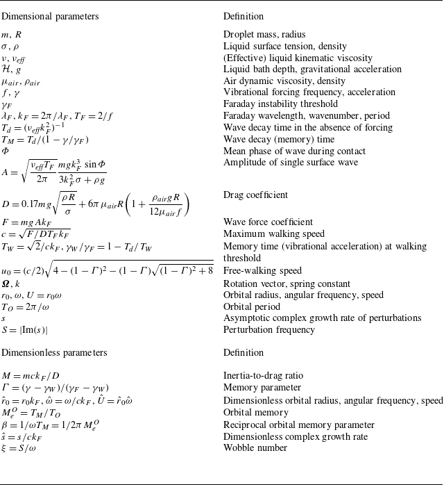
Table 1. Parameters appearing in the pilot-wave system (3.2) and subsequent analysis.
3.1. Integro-differential trajectory equation
The droplet’s horizontal motion is modelled using the stroboscopic trajectory equation developed by Oza et al. (Reference Oza, Rosales and Bush2013, Reference Oza, Harris, Rosales and Bush2014a
), as is deduced by time-averaging the dynamics over a bouncing period, $T_F$
(Moláček & Bush Reference Moláček and Bush2013). The droplet’s horizontal position,
$T_F$
(Moláček & Bush Reference Moláček and Bush2013). The droplet’s horizontal position, $\boldsymbol{x\!}_p(t)$
, thus evolves according to
$\boldsymbol{x\!}_p(t)$
, thus evolves according to
 \begin{equation} m\,\ddot {\!\boldsymbol{x}\!}_p + D\,\dot {\!\boldsymbol{x}\!}_p = -{mg\boldsymbol \nabla h(\boldsymbol{x\!}_p(t),t)} + \boldsymbol{F}, \end{equation}
where upper dots denote differentiation with respect to time, $t$
. The drop is propelled by the wave force,
$t$
. The drop is propelled by the wave force, $-mg \boldsymbol \nabla h({\boldsymbol{x}\!}_p, t)$
, and resisted by the linear drag force,
$-mg \boldsymbol \nabla h({\boldsymbol{x}\!}_p, t)$
, and resisted by the linear drag force, $-D\,\dot {\!\boldsymbol{x}\!}_p$
. We consider two different forms of the external force,
$-D\,\dot {\!\boldsymbol{x}\!}_p$
. We consider two different forms of the external force, $\boldsymbol{F}$
(see figure 1). For a droplet in a rotating frame, the droplet is subjected to a Coriolis force,
$\boldsymbol{F}$
(see figure 1). For a droplet in a rotating frame, the droplet is subjected to a Coriolis force, $\boldsymbol{F} = -2m\boldsymbol{\Omega }\times \,\dot {\!\boldsymbol{x}\!}_p$
, where
$\boldsymbol{F} = -2m\boldsymbol{\Omega }\times \,\dot {\!\boldsymbol{x}\!}_p$
, where $\boldsymbol{\Omega } = \Omega \boldsymbol{\hat {z}}$
is the vertical rotation vector. When the droplet is confined by an axisymmetric potential,
$\boldsymbol{\Omega } = \Omega \boldsymbol{\hat {z}}$
is the vertical rotation vector. When the droplet is confined by an axisymmetric potential, $V\!(|\boldsymbol{x}|)$
, the applied force is
$V\!(|\boldsymbol{x}|)$
, the applied force is $\boldsymbol{F} = -\boldsymbol \nabla V\!(|\boldsymbol{x\!}_p|)$
.
$\boldsymbol{F} = -\boldsymbol \nabla V\!(|\boldsymbol{x\!}_p|)$
.
The stroboscopic pilot wave,
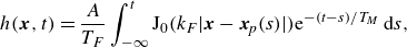 \begin{equation} h(\boldsymbol{x},t) = \frac {A}{T_F}\int _{-\infty }^t \textrm{J}_0(k_F|\boldsymbol{x} - \boldsymbol{x\!}_p(s)|)\textrm{e}^{-(t-s)/T_M}{\,\textrm{d}s}, \end{equation}
is modelled as a continuous superposition of axisymmetric waves of amplitude $A$
centred along the droplet’s path, decaying exponentially in time over the memory time scale,
$A$
centred along the droplet’s path, decaying exponentially in time over the memory time scale, $T_M = T_d/(1 - \gamma /\gamma _F)$
, where
$T_M = T_d/(1 - \gamma /\gamma _F)$
, where $T_d$
is the viscous decay time of the waves in the absence of vibrational forcing (Oza et al. Reference Oza, Rosales and Bush2013). The slower the waves decay, the greater the influence of the waves generated along the droplet’s path and so the longer the droplet’s path memory. Projecting the pilot wave onto the droplet’s path makes clear the influence of path memory on the droplet motion, as is encapsulated within the integro-differential trajectory equation (Oza et al. Reference Oza, Rosales and Bush2013, Reference Oza, Harris, Rosales and Bush2014a
)
$T_d$
is the viscous decay time of the waves in the absence of vibrational forcing (Oza et al. Reference Oza, Rosales and Bush2013). The slower the waves decay, the greater the influence of the waves generated along the droplet’s path and so the longer the droplet’s path memory. Projecting the pilot wave onto the droplet’s path makes clear the influence of path memory on the droplet motion, as is encapsulated within the integro-differential trajectory equation (Oza et al. Reference Oza, Rosales and Bush2013, Reference Oza, Harris, Rosales and Bush2014a
)
 \begin{align} \!\!\!\!\!m\,\ddot {\!\boldsymbol{x}\!}_p + \textit{D}\,\dot {\!\boldsymbol{x}\!}_p = \frac {F}{T_F}\int _{-\infty }^t \frac {\textrm{J}_1(k_F|\boldsymbol{x\!}_p(t) - {\boldsymbol{x}\!}_p(s)|)}{|\boldsymbol{x\!}_p(t) - \boldsymbol{x\!}_p(s)|}(\boldsymbol{x\!}_p(t) - \boldsymbol{x\!}_p(s))\textrm{e}^{-(t-s)/T_M}{\,\textrm{d}s} + \boldsymbol{F}, \end{align}
where $F = mgAk_F$
denotes the magnitude of the wave force. The quasi-monochromatic form of the pilot-wave field imposes a geometric constraint on the droplet’s motion whose effects are most pronounced at high memory, where the Faraday waves are most persistent.
$F = mgAk_F$
denotes the magnitude of the wave force. The quasi-monochromatic form of the pilot-wave field imposes a geometric constraint on the droplet’s motion whose effects are most pronounced at high memory, where the Faraday waves are most persistent.
Although the stroboscopic model (3.1) has adequately captured the majority of walker behaviours, it is based on the assumption that the droplet bounces in perfect resonance with the oscillation of the Faraday wave field. Recent work has demonstrated that significant non-resonant effects arise when droplets navigate a substantial wave field (Primkulov et al. Reference Primkulov, Evans, Been and Bush2025a ,Reference Primkulov, Evans, Frumkin, Sáenz and Bush b ); their role in orbital stability will be considered elsewhere. We also neglect the exponential far-field decay of the wave field (Tadrist et al. Reference Tadrist, Shim, Gilet and Schlagheck2018; Turton, Couchman & Bush Reference Turton, Couchman and Bush2018), which one expects to influence the stability of large circular orbits. Finally, we focus on small-amplitude perturbations from circular orbits; thus, our linear theory cannot lend insight into nonlinear effects as are responsible for the emergence of trefoil and lemniscate trajectories in a central force (Perrard et al. Reference Perrard, Labousse, Fort and Couder2014a ,Reference Perrard, Labousse, Miskin, Fort and Couder b ).
3.2. Memory and orbital memory
In the absence of an applied force, the droplet self-propels at a constant speed, $u_0(\gamma )$
, when the vibrational acceleration,
$u_0(\gamma )$
, when the vibrational acceleration, $\gamma$
, exceeds the walking threshold,
$\gamma$
, exceeds the walking threshold, $\gamma _W$
. As the vibrational forcing remains below the Faraday threshold in experiments,
$\gamma _W$
. As the vibrational forcing remains below the Faraday threshold in experiments, $\gamma \lt \gamma _F$
, it is convenient to characterise the pilot-wave dynamics in terms of the dimensionless memory parameter
$\gamma \lt \gamma _F$
, it is convenient to characterise the pilot-wave dynamics in terms of the dimensionless memory parameter $\Gamma = (\gamma - \gamma _W)/(\gamma _F - \gamma _W)$
(Bush Reference Bush2015; Oza, Rosales & Bush Reference Oza, Rosales and Bush2018). Notably,
$\Gamma = (\gamma - \gamma _W)/(\gamma _F - \gamma _W)$
(Bush Reference Bush2015; Oza, Rosales & Bush Reference Oza, Rosales and Bush2018). Notably, $\Gamma = 0$
corresponds to the walking threshold in the absence of an applied force (
$\Gamma = 0$
corresponds to the walking threshold in the absence of an applied force ( $\gamma = \gamma _W$
), while
$\gamma = \gamma _W$
), while $\Gamma = 1$
corresponds to the Faraday threshold (
$\Gamma = 1$
corresponds to the Faraday threshold ( $\gamma = \gamma _F$
), and thus infinite path memory. In addition,
$\gamma = \gamma _F$
), and thus infinite path memory. In addition, $\Gamma$
is related to the wave decay time,
$\Gamma$
is related to the wave decay time, $T_M$
, via
$T_M$
, via $\Gamma = 1 - T_W/T_M$
, where
$\Gamma = 1 - T_W/T_M$
, where $T_W$
is the memory time at the walking threshold,
$T_W$
is the memory time at the walking threshold, $\gamma _W$
(Durey et al. Reference Durey, Turton and Bush2020b
).
$\gamma _W$
(Durey et al. Reference Durey, Turton and Bush2020b
).
For orbital pilot-wave dynamics, a key concept is that of ‘orbital memory’ (Oza et al. Reference Oza, Harris, Rosales and Bush2014a
), which determines the extent to which an orbiting droplet interacts with its own wake, specifically the waves generated on its prior orbit. The longer the orbital memory, the more pronounced the self-potential. For a droplet moving in a circular orbit at angular frequency $\omega$
, the waves generated along the droplet path decay by a factor
$\omega$
, the waves generated along the droplet path decay by a factor $\textrm{e}^{-T_O/ T_M}$
over the orbital period,
$\textrm{e}^{-T_O/ T_M}$
over the orbital period, $T_O = 2\pi /\omega$
. We thus define
$T_O = 2\pi /\omega$
. We thus define $M_e^O = T_M/T_O$
as the orbital memory. When the droplet orbits close to its free-walking speed,
$M_e^O = T_M/T_O$
as the orbital memory. When the droplet orbits close to its free-walking speed, $u_0 \approx r_0 \omega$
, the orbital memory,
$u_0 \approx r_0 \omega$
, the orbital memory, $M_e^O \approx T_M u_0 /(2\pi r_0)$
, increases with vibrational forcing and decreases for larger orbits. For
$M_e^O \approx T_M u_0 /(2\pi r_0)$
, increases with vibrational forcing and decreases for larger orbits. For $M_e^O \ll 1$
, the wave decays quickly relative to the orbital period, so the droplet is largely unperturbed by its wake (see Appendix A). Conversely, if
$M_e^O \ll 1$
, the wave decays quickly relative to the orbital period, so the droplet is largely unperturbed by its wake (see Appendix A). Conversely, if $M_e^O \gg 1$
, the droplet is strongly influenced by its past history, with the quasi-monochromatic form of the Faraday wave field imposing a geometric constraint on the droplet motion. The onset of orbital instability arises at an intermediate regime,
$M_e^O \gg 1$
, the droplet is strongly influenced by its past history, with the quasi-monochromatic form of the Faraday wave field imposing a geometric constraint on the droplet motion. The onset of orbital instability arises at an intermediate regime, $M_e^O\approx 1$
(Oza et al. Reference Oza, Harris, Rosales and Bush2014a
). The precise dependence of this critical orbital memory on the orbital radius will be established in § 4.
$M_e^O\approx 1$
(Oza et al. Reference Oza, Harris, Rosales and Bush2014a
). The precise dependence of this critical orbital memory on the orbital radius will be established in § 4.
3.3. Orbital stability diagram
We begin by comparing the dynamics of circular orbits for the cases of a droplet propelling subject to a Coriolis force or confined by a linear spring force, $\boldsymbol{F} = -k \boldsymbol{x\!}_p$
. By substituting
$\boldsymbol{F} = -k \boldsymbol{x\!}_p$
. By substituting $\boldsymbol{x\!}_p(t) = r_0(\cos \omega t,\sin \omega t)$
into (3.2), we deduce the radial and tangential force balances
$\boldsymbol{x\!}_p(t) = r_0(\cos \omega t,\sin \omega t)$
into (3.2), we deduce the radial and tangential force balances
 \begin{align} -m r_0 \omega ^2 &= \frac {F}{T_F}\int _0^\infty \textrm{J}_1\left (2k_F r_0 \sin \left (\frac {\omega s}{2}\right )\right )\sin \left (\frac {\omega s}{2}\right )\textrm{e}^{-s/T_M}{\,\textrm{d}s} + \boldsymbol{F}\,{\boldsymbol\cdot}\, \boldsymbol{n}, \end{align}
 \begin{align} D r_0 \omega &= \frac {F}{T_F}\int _0^\infty \textrm{J}_1\left (2k_F r_0 \sin \left (\frac {\omega s}{2}\right )\right )\cos \left (\frac {\omega s}{2}\right )\textrm{e}^{-s/T_M}{\,\textrm{d}s} + \boldsymbol{F}\,{\boldsymbol\cdot}\, \boldsymbol{t}. \end{align}
Notably, the applied tangential force vanishes for droplet motion under the influence of either a Coriolis or a spring force, namely $\boldsymbol{F}\cdot \boldsymbol{t} = 0$
. Furthermore,
$\boldsymbol{F}\cdot \boldsymbol{t} = 0$
. Furthermore, $\boldsymbol{F}\cdot \boldsymbol{n} = 2m \Omega r_0 \omega$
for a Coriolis force and
$\boldsymbol{F}\cdot \boldsymbol{n} = 2m \Omega r_0 \omega$
for a Coriolis force and $\boldsymbol{F}\cdot \boldsymbol{n} = -kr_0$
for the linear spring force. We consider counter-clockwise orbital motion with
$\boldsymbol{F}\cdot \boldsymbol{n} = -kr_0$
for the linear spring force. We consider counter-clockwise orbital motion with $\omega \gt 0$
, so that
$\omega \gt 0$
, so that $U = r_0 \omega$
is the orbital speed. Owing to the droplet’s tendency to move along circular orbits at speeds close to the free-walking speed,
$U = r_0 \omega$
is the orbital speed. Owing to the droplet’s tendency to move along circular orbits at speeds close to the free-walking speed, $u_0$
(Bush et al. Reference Bush, Oza and Moláček2014), the orbital speed satisfies
$u_0$
(Bush et al. Reference Bush, Oza and Moláček2014), the orbital speed satisfies $U \approx u_0$
and is bounded above by the maximum steady walking speed, specifically that arising at the Faraday threshold,
$U \approx u_0$
and is bounded above by the maximum steady walking speed, specifically that arising at the Faraday threshold, $c = u_0(\gamma _F)$
(Liu et al. Reference Liu, Durey and Bush2023).
$c = u_0(\gamma _F)$
(Liu et al. Reference Liu, Durey and Bush2023).
In figure 3, we present the stability of circular orbits for a droplet moving in response to a Coriolis force or a linear spring force (the details of which are outlined in Appendices B and C). The orbital dynamics is parametrised by the memory parameter, $\Gamma$
, and the orbital radius,
$\Gamma$
, and the orbital radius, $r_0$
, which together determine the form of the Faraday wave field, or self-potential (Oza et al. Reference Oza, Harris, Rosales and Bush2014a
, Reference Oza, Rosales and Bush2018). The path memory endows the system with infinitely many eigenvalues. The stability of each orbit is thus characterised by the eigenvalue with largest real part (Oza et al. Reference Oza, Harris, Rosales and Bush2014a
), denoted
$r_0$
, which together determine the form of the Faraday wave field, or self-potential (Oza et al. Reference Oza, Harris, Rosales and Bush2014a
, Reference Oza, Rosales and Bush2018). The path memory endows the system with infinitely many eigenvalues. The stability of each orbit is thus characterised by the eigenvalue with largest real part (Oza et al. Reference Oza, Harris, Rosales and Bush2014a
), denoted $s_*$
, with the perturbation growing when
$s_*$
, with the perturbation growing when $\textrm{Re}(s_*) \gt 0$
and oscillating when
$\textrm{Re}(s_*) \gt 0$
and oscillating when $\textrm{Im}(s_*) \neq 0$
. At low memory, all orbits are found to be stable, as detailed in Appendix A (Oza Reference Oza2014). As the memory parameter is increased, stable circular orbits (blue) destabilise progressively via either monotonically growing (red) or wobbling (green or orange) instability mechanisms. Stable circular orbits are thus quantised in radius at high memory, corresponding to the blue plateaus in figure 3(a,b). We summarise the orbital stability for all values of
$\textrm{Im}(s_*) \neq 0$
. At low memory, all orbits are found to be stable, as detailed in Appendix A (Oza Reference Oza2014). As the memory parameter is increased, stable circular orbits (blue) destabilise progressively via either monotonically growing (red) or wobbling (green or orange) instability mechanisms. Stable circular orbits are thus quantised in radius at high memory, corresponding to the blue plateaus in figure 3(a,b). We summarise the orbital stability for all values of $\Gamma$
in the stability diagram (figure 3
c,d), where instabilities appear as ‘tongues’ separating intervals of quantised stable radii.
$\Gamma$
in the stability diagram (figure 3
c,d), where instabilities appear as ‘tongues’ separating intervals of quantised stable radii.
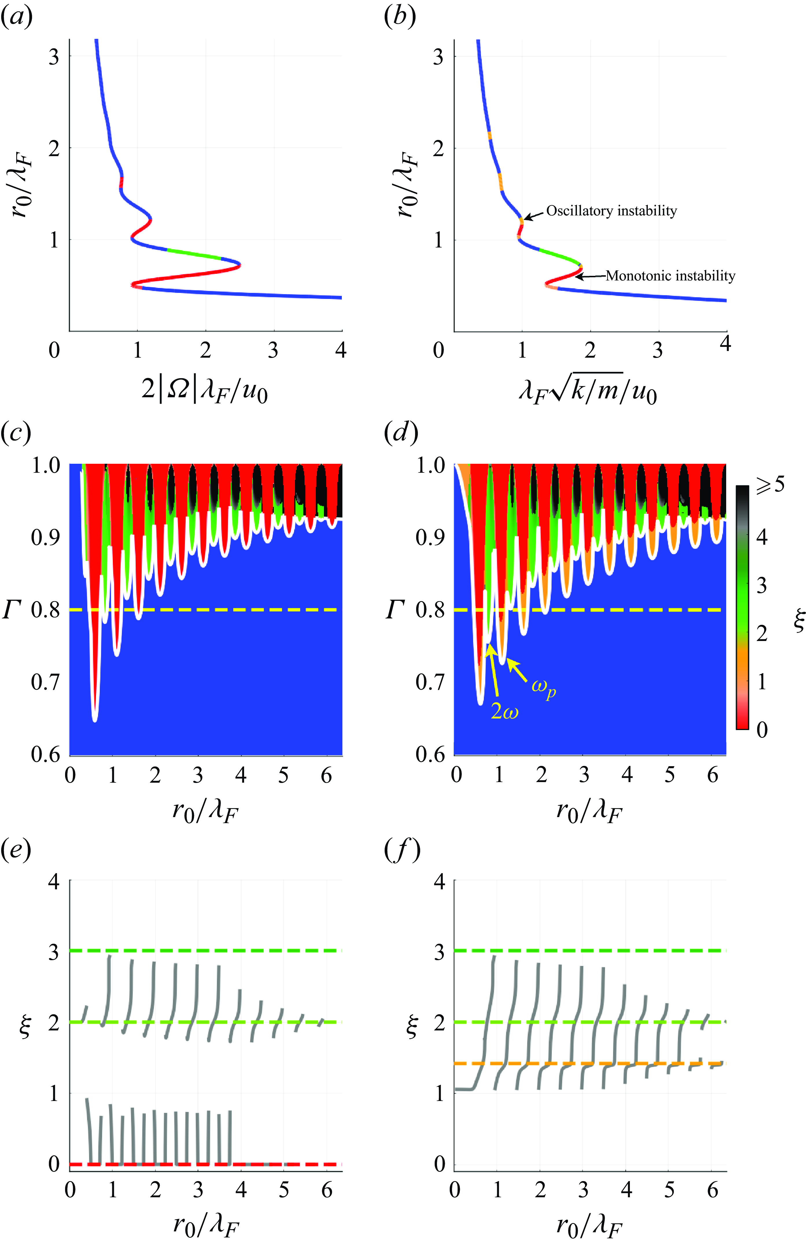
Figure 3. Stability of circular orbits for (a,c,e) a Coriolis force and (b,d,f) a linear spring force. (a,b) Relationship between the orbital radius, $r_0$
, and (a) the rotation rate,
$r_0$
, and (a) the rotation rate, $\Omega$
, or (b) the spring constant,
$\Omega$
, or (b) the spring constant, $k$
, for circular orbits with memory parameter
$k$
, for circular orbits with memory parameter $\Gamma = 0.8$
. Blue portions of the curve denote stable circular orbits, with red, green and orange indicating unstable orbits, colour-coded by the corresponding wobble number,
$\Gamma = 0.8$
. Blue portions of the curve denote stable circular orbits, with red, green and orange indicating unstable orbits, colour-coded by the corresponding wobble number, $\xi = S/\omega$
. (c,d) Orbital stability diagram for a range of
$\xi = S/\omega$
. (c,d) Orbital stability diagram for a range of $\Gamma$
, with the yellow dashed line corresponding to the orbital curve in panels (a,b). The white curve denotes the stability boundary, above which all circular orbits are unstable. Quantised orbits emerge between the instability tongues. We note the additional orange regions in panel (d), corresponding to
$\Gamma$
, with the yellow dashed line corresponding to the orbital curve in panels (a,b). The white curve denotes the stability boundary, above which all circular orbits are unstable. Quantised orbits emerge between the instability tongues. We note the additional orange regions in panel (d), corresponding to $\omega _p = \sqrt {2}\omega$
instabilities. (e,f) Dependence of the wobble number,
$\omega _p = \sqrt {2}\omega$
instabilities. (e,f) Dependence of the wobble number, $\xi$
(grey curve), along the stability boundary (white curve in panels c,d). Discontinuities in
$\xi$
(grey curve), along the stability boundary (white curve in panels c,d). Discontinuities in $\xi$
correspond to changes in the instability mechanism. The dashed lines correspond to
$\xi$
correspond to changes in the instability mechanism. The dashed lines correspond to $\xi = 0$
,
$\xi = 0$
, $\xi = \sqrt {2}$
,
$\xi = \sqrt {2}$
, $\xi = 2$
and
$\xi = 2$
and $\xi = 3$
. Monotonic instabilities are subdominant to potential-driven instabilities for a linear spring force and so are not evident in panel (f).
$\xi = 3$
. Monotonic instabilities are subdominant to potential-driven instabilities for a linear spring force and so are not evident in panel (f).
We characterise the dependence of the instability mechanism on the orbital radius in terms of the wobble number, $\xi = S/\omega$
, defined as the ratio of the instability frequency,
$\xi = S/\omega$
, defined as the ratio of the instability frequency, $S = |\textrm{Im}(s_*)|$
, to the orbital frequency,
$S = |\textrm{Im}(s_*)|$
, to the orbital frequency, $\omega$
. The wobble number on the stability boundary (denoted by the white curve in figure 3
c,d) varies significantly with the orbital radius, as is evident from the grey curves in figure 3(e,f). Discontinuities in
$\omega$
. The wobble number on the stability boundary (denoted by the white curve in figure 3
c,d) varies significantly with the orbital radius, as is evident from the grey curves in figure 3(e,f). Discontinuities in $\xi$
correspond to changes in the instability mechanism. Specifically,
$\xi$
correspond to changes in the instability mechanism. Specifically, $\xi$
switches between intervals of monotonic instabilities (
$\xi$
switches between intervals of monotonic instabilities ( $\xi = 0$
) and wobbling instabilities (
$\xi = 0$
) and wobbling instabilities ( $\xi \gt 0$
) as
$\xi \gt 0$
) as $r_0$
increases over a length scale comparable to half the Faraday wavelength. As is summarised in table 2, the instability mechanism alternates between monotonic instabilities and 2-wobbles for a Coriolis force (Oza et al. Reference Oza, Harris, Rosales and Bush2014a
,Reference Oza, Wind-Willassen, Harris, Rosales and Bush
b
). For a linear spring force, monotonic instabilities are subdominant to wobbling instabilities at frequencies
$r_0$
increases over a length scale comparable to half the Faraday wavelength. As is summarised in table 2, the instability mechanism alternates between monotonic instabilities and 2-wobbles for a Coriolis force (Oza et al. Reference Oza, Harris, Rosales and Bush2014a
,Reference Oza, Wind-Willassen, Harris, Rosales and Bush
b
). For a linear spring force, monotonic instabilities are subdominant to wobbling instabilities at frequencies $2\omega$
(green) and
$2\omega$
(green) and $\omega _p = \sqrt {2}\omega$
(orange; see § 2.2), corresponding to resonant wave-driven 2-wobbles (Harris & Bush Reference Harris and Bush2014) and non-resonant potential-driven wobbling, respectively.
$\omega _p = \sqrt {2}\omega$
(orange; see § 2.2), corresponding to resonant wave-driven 2-wobbles (Harris & Bush Reference Harris and Bush2014) and non-resonant potential-driven wobbling, respectively.
Despite the complexity of the orbital stability problem, monotonic instabilities have a particularly simple form. Specifically, circular orbits have an unstable real eigenvalue (corresponding to monotonic growth) in the upward-sloping portions of the orbital solution curves in figure 3(a,b); see Theorem 1 of Oza et al. (Reference Oza, Harris, Rosales and Bush2014a ) for a proof in the case of a Coriolis force and Theorem1 (Appendix B) for a generalised proof applicable to both Coriolis and central forces. For a Coriolis force, these monotonic instabilities are responsible for the onset of orbital quantisation. For a linear spring force, however, monotonic instabilities are subdominant to potential-driven wobbling, which instead drive the onset of orbital quantisation.
Two further instabilities, common to both the Coriolis force and the linear spring force, are evident in figure 3. First, we note that the wobble number, $\xi$
, approaches 3 when
$\xi$
, approaches 3 when $r_0/\lambda _F$
is just below a half-integer multiple of the Faraday wavelength for small orbits (see figure 3
e,f). This instability corresponds to the 3-wobbles identified in the numerical simulations of Oza et al. (Reference Oza, Wind-Willassen, Harris, Rosales and Bush2014b
) within small portions of parameter space, but they have proven to be elusive in the laboratory (Harris & Bush Reference Harris and Bush2014). Second, we note that large values of the wobble number (
$r_0/\lambda _F$
is just below a half-integer multiple of the Faraday wavelength for small orbits (see figure 3
e,f). This instability corresponds to the 3-wobbles identified in the numerical simulations of Oza et al. (Reference Oza, Wind-Willassen, Harris, Rosales and Bush2014b
) within small portions of parameter space, but they have proven to be elusive in the laboratory (Harris & Bush Reference Harris and Bush2014). Second, we note that large values of the wobble number ( $\xi \geqslant 5$
) are evident in the black portions of figure 3(c,d), appearing only at high memory. This instability corresponds to speed oscillations over a length scale comparable to the Faraday wavelength (Bacot et al. Reference Bacot, Perrard, Labousse, Couder and Fort2019; Hubert et al. Reference Hubert, Labousse, Perrard, Labousse, Vandewalle and Couder2019; Durey et al. Reference Durey, Turton and Bush2020b
), for which
$\xi \geqslant 5$
) are evident in the black portions of figure 3(c,d), appearing only at high memory. This instability corresponds to speed oscillations over a length scale comparable to the Faraday wavelength (Bacot et al. Reference Bacot, Perrard, Labousse, Couder and Fort2019; Hubert et al. Reference Hubert, Labousse, Perrard, Labousse, Vandewalle and Couder2019; Durey et al. Reference Durey, Turton and Bush2020b
), for which $\xi \approx r_0 k_F$
(Liu et al. Reference Liu, Durey and Bush2023). For orbits larger than those presented in figure 3 (i.e. for
$\xi \approx r_0 k_F$
(Liu et al. Reference Liu, Durey and Bush2023). For orbits larger than those presented in figure 3 (i.e. for $r_0/\lambda _F \gt 6$
), these speed oscillations form the dominant instability mechanism, in accordance with the instability of rectilinear walkers (Durey et al. Reference Durey, Turton and Bush2020b
). Owing to the relative scarcity of both 3-wobbles and speed oscillations in the laboratory, we henceforth focus our investigation on monotonically growing perturbations and wave- and potential-driven wobbling.
$r_0/\lambda _F \gt 6$
), these speed oscillations form the dominant instability mechanism, in accordance with the instability of rectilinear walkers (Durey et al. Reference Durey, Turton and Bush2020b
). Owing to the relative scarcity of both 3-wobbles and speed oscillations in the laboratory, we henceforth focus our investigation on monotonically growing perturbations and wave- and potential-driven wobbling.
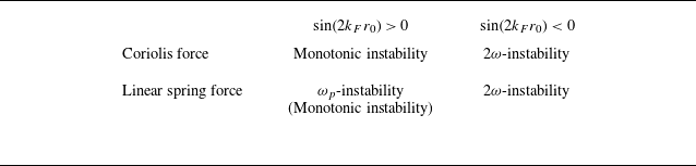
Table 2. Correspondence between the sign of $\sin (2 k_F r_0)$
and the existence of monotonic or wobbling instabilities (at frequency
$\sin (2 k_F r_0)$
and the existence of monotonic or wobbling instabilities (at frequency $2\omega$
or
$2\omega$
or $\omega _p = \sqrt {2}\omega$
) for orbital motion with radius
$\omega _p = \sqrt {2}\omega$
) for orbital motion with radius $r_0$
and frequency
$r_0$
and frequency $\omega$
subjected to a Coriolis force or a linear spring force. Subdominant instabilities are denoted in parentheses. These results are deduced from the asymptotic analysis in § 4.
$\omega$
subjected to a Coriolis force or a linear spring force. Subdominant instabilities are denoted in parentheses. These results are deduced from the asymptotic analysis in § 4.
4. Onset of instability
We proceed to develop asymptotic formulae for the critical memory and frequency of instability for large circular orbits, which we use to explain the structural differences in the stability diagram for different external forces. Motivated by the effective radial force fields inferred for droplet–topography interactions and by the differences in the orbital stability diagram enumerated in § 3.3, we broaden our analysis to encompass the cases of a Coriolis force, $\boldsymbol{F} = -2m \boldsymbol{\Omega } \times \,\dot {\!\boldsymbol{x}\!}_p$
, and a power-law central force of the form
$\boldsymbol{F} = -2m \boldsymbol{\Omega } \times \,\dot {\!\boldsymbol{x}\!}_p$
, and a power-law central force of the form $\boldsymbol{F} = -k|\boldsymbol{x\!}_p|^{n-1}\boldsymbol{x\!}_p$
, where
$\boldsymbol{F} = -k|\boldsymbol{x\!}_p|^{n-1}\boldsymbol{x\!}_p$
, where $k$
is the spring constant. Notably, the central force may be derived from a power-law potential of the form
$k$
is the spring constant. Notably, the central force may be derived from a power-law potential of the form $V\!(r) \propto r^{n+1}$
when
$V\!(r) \propto r^{n+1}$
when $n \gt -1$
, and from a logarithmic potential,
$n \gt -1$
, and from a logarithmic potential, $V\!(r) \propto \ln (r)$
, when
$V\!(r) \propto \ln (r)$
, when $n = -1$
. We pay particular attention to the case of
$n = -1$
. We pay particular attention to the case of $n+1$
being a perfect square, for which potential-driven wobbling with frequency
$n+1$
being a perfect square, for which potential-driven wobbling with frequency $\omega _p = \omega \sqrt {n+1}$
resonates with the orbital frequency, leading to a stability diagram of more complex structure. As most circular orbits are found to be unstable with monotonically growing perturbations for
$\omega _p = \omega \sqrt {n+1}$
resonates with the orbital frequency, leading to a stability diagram of more complex structure. As most circular orbits are found to be unstable with monotonically growing perturbations for $n \lt -1$
(in accordance with
$n \lt -1$
(in accordance with $\omega _p$
being imaginary), we consider
$\omega _p$
being imaginary), we consider $n \geqslant -1$
henceforth. We also restrict our attention to
$n \geqslant -1$
henceforth. We also restrict our attention to $n\leqslant 4$
for the sake of brevity.
$n\leqslant 4$
for the sake of brevity.
To investigate the onset of orbital instability, we leverage linear stability analysis to determine the response of the droplet trajectory when perturbed from a circular orbit following an impulsive force. The linear stability framework is outlined in Appendices B and C, and is derived by taking Laplace transforms of the linearised droplet trajectory equation. The poles of the resultant transfer function correspond to the long-time asymptotic growth rates, $s$
(Oza et al. Reference Oza, Harris, Rosales and Bush2014a
). A key feature of our framework is that the radial force balance (3.3a
) is used to eliminate the applied force as a parameter in the stability problem. Instead, orbits are parametrised by their radius (Oza Reference Oza2014; Oza et al. Reference Oza, Harris, Rosales and Bush2014a
; Liu et al. Reference Liu, Durey and Bush2023), with the corresponding orbital frequency deduced from the tangential force balance (3.3b
).
$s$
(Oza et al. Reference Oza, Harris, Rosales and Bush2014a
). A key feature of our framework is that the radial force balance (3.3a
) is used to eliminate the applied force as a parameter in the stability problem. Instead, orbits are parametrised by their radius (Oza Reference Oza2014; Oza et al. Reference Oza, Harris, Rosales and Bush2014a
; Liu et al. Reference Liu, Durey and Bush2023), with the corresponding orbital frequency deduced from the tangential force balance (3.3b
).
4.1. Asymptotic framework
We here develop an asymptotic framework for analysing the stability of large circular orbits, for which $r_0 k_F \gg 1$
, building upon the analysis of Liu et al. (Reference Liu, Durey and Bush2023) for orbiting in a rotating frame. In so doing, we determine asymptotic formulae for the critical vibrational acceleration along the stability boundary and the corresponding instability frequency,
$r_0 k_F \gg 1$
, building upon the analysis of Liu et al. (Reference Liu, Durey and Bush2023) for orbiting in a rotating frame. In so doing, we determine asymptotic formulae for the critical vibrational acceleration along the stability boundary and the corresponding instability frequency, $S$
. These formulae may then be used to compare the relative vibrational forcing at which instabilities occur, as well as the corresponding orbital radii at the tip of each instability tongue. One key inference made from our analysis is the peculiar switching in the structure of the stability boundaries as the force power,
$S$
. These formulae may then be used to compare the relative vibrational forcing at which instabilities occur, as well as the corresponding orbital radii at the tip of each instability tongue. One key inference made from our analysis is the peculiar switching in the structure of the stability boundaries as the force power, $n$
, is varied. This switching demonstrates limitations in prior heuristic arguments for predicting the critical radii of instability tongues solely in terms of zeros of Bessel functions (Labousse et al. Reference Labousse, Oza, Perrard and Bush2016), the wave energy (Durey Reference Durey2018) or the structure of the mean wave field (Liu et al. Reference Liu, Durey and Bush2023).
$n$
, is varied. This switching demonstrates limitations in prior heuristic arguments for predicting the critical radii of instability tongues solely in terms of zeros of Bessel functions (Labousse et al. Reference Labousse, Oza, Perrard and Bush2016), the wave energy (Durey Reference Durey2018) or the structure of the mean wave field (Liu et al. Reference Liu, Durey and Bush2023).
Central to our analysis is determining suitable scaling relationships between the dimensionless radius, $\hat {r}_0 = k_F r_0 \gg 1$
, the dimensionless orbital speed,
$\hat {r}_0 = k_F r_0 \gg 1$
, the dimensionless orbital speed, $\hat {U} = U/c$
, the wobble number,
$\hat {U} = U/c$
, the wobble number, $\xi = S/\omega$
, and the reciprocal orbital memory parameter,
$\xi = S/\omega$
, and the reciprocal orbital memory parameter, $\beta = 1/(\omega T_M)$
, which may be equivalently defined as
$\beta = 1/(\omega T_M)$
, which may be equivalently defined as $\beta = 1/(2\pi M_e^O)$
. We recall that
$\beta = 1/(2\pi M_e^O)$
. We recall that $U \lt c$
for all orbits, with
$U \lt c$
for all orbits, with $U$
generally quite close to
$U$
generally quite close to $c$
at high memory, and so assume that
$c$
at high memory, and so assume that $\hat {U} = O(1)$
. Furthermore, as we are investigating monotonic and wobbling instabilities, we assume that
$\hat {U} = O(1)$
. Furthermore, as we are investigating monotonic and wobbling instabilities, we assume that $\xi = O(1)$
, with the leading-order contribution (and thus wobble number) arising naturally from our analysis. Furthermore, we observe from figure 4 that the wave damping factor over half an orbital period,
$\xi = O(1)$
, with the leading-order contribution (and thus wobble number) arising naturally from our analysis. Furthermore, we observe from figure 4 that the wave damping factor over half an orbital period, $\textrm{e}^{-\pi \beta } = \textrm{e}^{-T_O/2T_M}$
, scales algebraically with radius along the stability boundary for a linear spring force. Specifically,
$\textrm{e}^{-\pi \beta } = \textrm{e}^{-T_O/2T_M}$
, scales algebraically with radius along the stability boundary for a linear spring force. Specifically, $2\omega$
-instabilities (green line) satisfy the scaling
$2\omega$
-instabilities (green line) satisfy the scaling $\textrm{e}^{-\pi \beta } = O(\hat {r}_0^{-2})$
and
$\textrm{e}^{-\pi \beta } = O(\hat {r}_0^{-2})$
and $\omega _p$
-instabilities (orange line) satisfy
$\omega _p$
-instabilities (orange line) satisfy $\textrm{e}^{-\pi \beta } = O(\hat {r}_0^{-3})$
. The scaling relationship
$\textrm{e}^{-\pi \beta } = O(\hat {r}_0^{-3})$
. The scaling relationship $\textrm{e}^{-\pi \beta } = O(\hat {r}_0^{-2})$
also arises for monotonic and
$\textrm{e}^{-\pi \beta } = O(\hat {r}_0^{-2})$
also arises for monotonic and $2\omega$
-instabilities in a Coriolis force (Liu et al. Reference Liu, Durey and Bush2023), and we find that similar scaling relationships emerge for nonlinear springs. To account for all of these cases, we assume that the dominant balance
$2\omega$
-instabilities in a Coriolis force (Liu et al. Reference Liu, Durey and Bush2023), and we find that similar scaling relationships emerge for nonlinear springs. To account for all of these cases, we assume that the dominant balance $\beta = O(\ln \hat {r}_0)$
holds for
$\beta = O(\ln \hat {r}_0)$
holds for $\hat {r}_0 \gg 1$
, with the particular scaling power
$\hat {r}_0 \gg 1$
, with the particular scaling power $\textrm{e}^{-\pi \beta } = O(\hat {r}_0^{-l})$
being deduced as part of the solution process detailed in Appendix D. We summarise the results of this analysis as follows.
$\textrm{e}^{-\pi \beta } = O(\hat {r}_0^{-l})$
being deduced as part of the solution process detailed in Appendix D. We summarise the results of this analysis as follows.
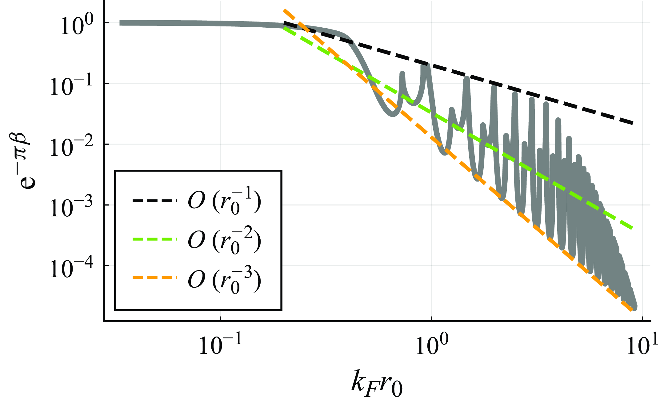
Figure 4. Dependence of the wave damping factor over half an orbital period, denoted $\textrm{e}^{-\pi \beta } = \textrm{e}^{-T_O/(2T_M)}$
, at the onset of instability on the orbital radius,
$\textrm{e}^{-\pi \beta } = \textrm{e}^{-T_O/(2T_M)}$
, at the onset of instability on the orbital radius, $r_0$
, for a linear central force,
$r_0$
, for a linear central force, $\boldsymbol{F} = -k\boldsymbol{x\!}_p$
(
$\boldsymbol{F} = -k\boldsymbol{x\!}_p$
( $n = 1$
). The grey curve is a rescaling of the stability boundary (white curve) presented in figure 3(d). Notably, the envelopes of the instability tongues satisfy the scaling
$n = 1$
). The grey curve is a rescaling of the stability boundary (white curve) presented in figure 3(d). Notably, the envelopes of the instability tongues satisfy the scaling $\textrm{e}^{-\pi \beta } = O(\hat {r}_0^{-l})$
for
$\textrm{e}^{-\pi \beta } = O(\hat {r}_0^{-l})$
for $l = 2$
and
$l = 2$
and $l = 3$
, which are used in the asymptotic analysis presented in § 4.1. The scaling
$l = 3$
, which are used in the asymptotic analysis presented in § 4.1. The scaling $\textrm{e}^{-\pi \beta } = O(\hat {r}_0^{-1})$
emerges between pairs of instability tongues, including for 3-wobbles, but is outside the scope of this investigation.
$\textrm{e}^{-\pi \beta } = O(\hat {r}_0^{-1})$
emerges between pairs of instability tongues, including for 3-wobbles, but is outside the scope of this investigation.
4.2. Walking in a rotating frame
Liu et al. (Reference Liu, Durey and Bush2023) demonstrated that orbiting in a Coriolis force gives rise to monotonic and $2\omega$
-instabilities as the vibrational forcing is increased. In terms of the dimensionless mass,
$2\omega$
-instabilities as the vibrational forcing is increased. In terms of the dimensionless mass, $M = mck_F/D$
, and reciprocal orbital memory parameter,
$M = mck_F/D$
, and reciprocal orbital memory parameter, $\beta$
, the leading-order approximation for the stability boundary corresponding to monotonic instabilities is
$\beta$
, the leading-order approximation for the stability boundary corresponding to monotonic instabilities is
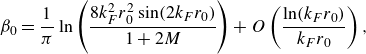 \begin{equation} \beta _{0} = \frac {1}{\pi }\ln \left (\frac {8 k_F^2 r_0^2\sin (2 k_F r_0)}{1 + 2M}\right ) + O\left (\frac {\ln ( k_F r_0)}{k_F r_0}\right ), \end{equation}
which is valid when $\sin (2k_F r_0) \approx 1$
. Notably, maxima in
$\sin (2k_F r_0) \approx 1$
. Notably, maxima in $\beta$
correspond to minima in
$\beta$
correspond to minima in $\Gamma$
(where
$\Gamma$
(where $\Gamma = 1- \sqrt {2}\omega \beta / c k_F$
along stability boundaries), which represent the tips of the instability tongues in figure 3(c). Similarly, the stability boundary corresponding to
$\Gamma = 1- \sqrt {2}\omega \beta / c k_F$
along stability boundaries), which represent the tips of the instability tongues in figure 3(c). Similarly, the stability boundary corresponding to $2\omega$
-instabilities is
$2\omega$
-instabilities is
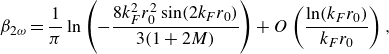 \begin{equation} \beta _{2\omega } = \frac {1}{\pi }\ln \left (-\frac {8 k_F^2 r_0^2\sin (2 k_F r_0)}{3(1 + 2M)}\right ) + O\left (\frac {\ln (k_F r_0)}{k_F r_0}\right ), \end{equation}
valid when $\sin (2k_Fr_0) \approx -1$
, where the corresponding wobble number along the stability boundary is
$\sin (2k_Fr_0) \approx -1$
, where the corresponding wobble number along the stability boundary is
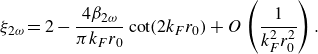 \begin{equation} \xi _{2\omega } = 2 - \frac {4\beta _{2\omega }}{\pi k_F r_0}\cot (2k_F r_0) + O\left (\frac {1}{k_F^2 r_0^2}\right ). \end{equation}
The monotonic and 2-wobble instabilities are thus interlaced, with the corresponding instability tongues in figure 3(c) alternating over half the Faraday wavelength as the orbital radius is increased. As the critical radii, which lie at the tip of each instability tongue, approximately satisfy $\cos (2k_Fr_0) = 0$
for large orbits, the
$\cos (2k_Fr_0) = 0$
for large orbits, the $O(1/k_Fr_0)$
correction to
$O(1/k_Fr_0)$
correction to $\xi _{2\omega }$
vanishes at the tip of each instability tongue, giving rise to
$\xi _{2\omega }$
vanishes at the tip of each instability tongue, giving rise to $\xi = 2 + O (1/k_F^2 r_0^2 )$
. We note also that increasing the dimensionless mass,
$\xi = 2 + O (1/k_F^2 r_0^2 )$
. We note also that increasing the dimensionless mass, $M$
, increases the critical memory of instability, corresponding to shortening of the instability tongues in the stability diagram.
$M$
, increases the critical memory of instability, corresponding to shortening of the instability tongues in the stability diagram.
4.3. Walking in a power-law central force
For orbital motion in a power-law central force, $\boldsymbol{F} = -k|\boldsymbol{x\!}_p|^{n-1}\boldsymbol{x\!}_p$
, corresponding to
$\boldsymbol{F} = -k|\boldsymbol{x\!}_p|^{n-1}\boldsymbol{x\!}_p$
, corresponding to $V\!(r) \propto r^{n+1}$
for
$V\!(r) \propto r^{n+1}$
for $n \gt -1$
, the onset of instability is more intricate, with a subtle dependence of the instability mechanism on the force power,
$n \gt -1$
, the onset of instability is more intricate, with a subtle dependence of the instability mechanism on the force power, $n$
(see Appendix D). We detail the onset of wave- and potential-driven instabilities as follows.
$n$
(see Appendix D). We detail the onset of wave- and potential-driven instabilities as follows.
4.3.1. Wave-driven instabilities
For wave-driven resonant instabilities, the wobble number is $\xi \approx 2N$
for any integer
$\xi \approx 2N$
for any integer $N \geqslant 0$
, with
$N \geqslant 0$
, with $N = 0$
for monotonic instabilities and
$N = 0$
for monotonic instabilities and $N = 1$
for 2-wobbles. The reciprocal orbital memory parameter along the stability boundary (corresponding to
$N = 1$
for 2-wobbles. The reciprocal orbital memory parameter along the stability boundary (corresponding to $\Gamma = 1- \sqrt {2}\omega \beta / c k_F$
) is
$\Gamma = 1- \sqrt {2}\omega \beta / c k_F$
) is
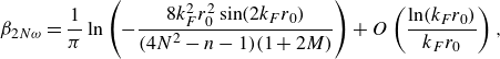 \begin{equation} \beta _{2N\omega } = \frac {1}{\pi }\ln \left (-\frac {8k_F^2 r_0^2\sin (2 k_F r_0)}{(4N^2-n-1)(1 + 2M)}\right ) + O\left (\frac {\ln (k_F r_0)}{k_F r_0}\right ), \end{equation}
which is valid provided that $|\sin (2k_F r_0)| = O(1)$
and the argument of the logarithm is positive. The corresponding wobble number along the stability boundary is
$|\sin (2k_F r_0)| = O(1)$
and the argument of the logarithm is positive. The corresponding wobble number along the stability boundary is
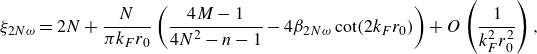 \begin{equation} \xi _{2N\omega } = 2N + \frac {N}{\pi k_F r_0}\left (\frac {4M-1}{4N^2-n-1} - 4\beta _{2N\omega }\cot (2 k_F r_0)\right ) + O\left (\frac {1}{k_F^2 r_0^2}\right ), \end{equation}
where $\xi _0 = 0$
for monotonic instabilities.
$\xi _0 = 0$
for monotonic instabilities.
There are two notable similarities in the onset of wave-driven instabilities for the Coriolis and power-law central forces. First, both systems satisfy the asymptotic scaling $\textrm{e}^{-\pi \beta } = O(\hat {r}_0^{-2})$
. Second, wobbling instabilities with
$\textrm{e}^{-\pi \beta } = O(\hat {r}_0^{-2})$
. Second, wobbling instabilities with $N \gt 1$
are subdominant to monotonic (
$N \gt 1$
are subdominant to monotonic ( $N = 0$
) and
$N = 0$
) and $2\omega$
(
$2\omega$
( $N = 1$
) instabilities in both systems for all
$N = 1$
) instabilities in both systems for all $M \gt 0$
, as was shown by Liu et al. (Reference Liu, Durey and Bush2023) for a Coriolis force. For a central force, this result may be verified by using (4.2a
) to deduce that the leading-order stability envelope is defined as
$M \gt 0$
, as was shown by Liu et al. (Reference Liu, Durey and Bush2023) for a Coriolis force. For a central force, this result may be verified by using (4.2a
) to deduce that the leading-order stability envelope is defined as
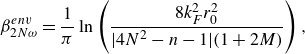 \begin{equation} \beta _{2N\omega }^{{env}} = \frac {1}{\pi }\ln \left (\frac {8 k_F^2 r_0^2}{|4N^2 - n - 1|(1 + 2M)}\right ), \end{equation}
which is found by substituting $|\sin (2k_F r_0)| = 1$
into (4.2a
). The critical memory of instability is thus lower for smaller values of
$|\sin (2k_F r_0)| = 1$
into (4.2a
). The critical memory of instability is thus lower for smaller values of $|4N^2 - n - 1|$
, with the two smallest values achieved for
$|4N^2 - n - 1|$
, with the two smallest values achieved for $N = 0$
and
$N = 0$
and $N = 1$
for the range of force powers (
$N = 1$
for the range of force powers ( $-1 \lt n \leqslant 4$
) considered here.
$-1 \lt n \leqslant 4$
) considered here.
Two important differences in the onset of wave-driven instabilities between the two systems are also apparent. First, the factor of $4N^2 - n - 1$
in (4.2a
) changes sign for larger
$4N^2 - n - 1$
in (4.2a
) changes sign for larger $n$
, causing
$n$
, causing $2\omega$
-instabilities to overlap with monotonic instabilities in the stability diagram for a central force with
$2\omega$
-instabilities to overlap with monotonic instabilities in the stability diagram for a central force with $n \gt 3$
(see table 3 and § 4.3.4). Second, the additional
$n \gt 3$
(see table 3 and § 4.3.4). Second, the additional $O(1/k_Fr_0)$
frequency detuning term in (4.2b
) leads to an appreciable departure from an exact 2-wobble at the onset of instability relative to a Coriolis force (see 4.1c
), as was evident in the simulations of Tambasco et al. (Reference Tambasco, Harris, Oza, Rosales and Bush2016, figure 7a) close the stability boundary.
$O(1/k_Fr_0)$
frequency detuning term in (4.2b
) leads to an appreciable departure from an exact 2-wobble at the onset of instability relative to a Coriolis force (see 4.1c
), as was evident in the simulations of Tambasco et al. (Reference Tambasco, Harris, Oza, Rosales and Bush2016, figure 7a) close the stability boundary.
Table 3. Correspondence between the sign of $\sin (2 k_F r_0)$
and the existence of monotonic and wobbling instabilities (at frequency
$\sin (2 k_F r_0)$
and the existence of monotonic and wobbling instabilities (at frequency $2\omega$
or
$2\omega$
or $\omega _p = \omega \sqrt {n+1}$
) for a droplet walking in a power-law central force,
$\omega _p = \omega \sqrt {n+1}$
) for a droplet walking in a power-law central force, $\boldsymbol{F} = -k|\boldsymbol{x\!}_p|^{n-1}\boldsymbol{x\!}_p$
. These results may be deduced by requiring the argument of the corresponding logarithm in (4.2a
) or (4.4a
) to be positive. Subdominant instabilities are indicated in parentheses. We restrict our attention to
$\boldsymbol{F} = -k|\boldsymbol{x\!}_p|^{n-1}\boldsymbol{x\!}_p$
. These results may be deduced by requiring the argument of the corresponding logarithm in (4.2a
) or (4.4a
) to be positive. Subdominant instabilities are indicated in parentheses. We restrict our attention to $-1 \lt n \leqslant 4$
and to the parameters accessible in experiments (for which the dimensionless mass satisfies
$-1 \lt n \leqslant 4$
and to the parameters accessible in experiments (for which the dimensionless mass satisfies $4M \gt 1$
).
$4M \gt 1$
).
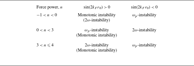
4.3.2. Potential-driven instabilities
The stability boundary corresponding to potential-driven wobbling involves the distinct scaling of $\textrm{e}^{-\pi \beta } = O(\hat {r}_0^{-3})$
(see Appendix D), with
$\textrm{e}^{-\pi \beta } = O(\hat {r}_0^{-3})$
(see Appendix D), with
 \begin{equation} \beta _{\omega _p} = \frac {1}{\pi }\log \left (-\frac {16 k_F^3 r_0^3\sin (2 k_F r_0)\sin (\pi \xi _{\omega _p})}{\xi _{\omega _p}(4M - 1)(2M + 1)}\right ) \end{equation}
along the stability boundary to leading order. As our analysis is focused on the parameter regime accessible in the laboratory (Harris & Bush Reference Harris and Bush2014), for which $M \approx 2.27$
, we henceforth restrict our attention to the case
$M \approx 2.27$
, we henceforth restrict our attention to the case $4M \gt 1$
. Consequently, (4.4a
) is valid provided that (i)
$4M \gt 1$
. Consequently, (4.4a
) is valid provided that (i) $|\sin (2k_Fr_0)|\approx 1$
and (ii)
$|\sin (2k_Fr_0)|\approx 1$
and (ii) $\sin (2k_Fr_0)$
and
$\sin (2k_Fr_0)$
and $\sin (\pi \xi _{\omega _p})$
are of opposite signs. Finally,
$\sin (\pi \xi _{\omega _p})$
are of opposite signs. Finally,
 \begin{equation} \xi _{\omega _p} = \sqrt {n+1} + o(1) \end{equation}
is the leading-order instability frequency, which corresponds precisely to the perturbation frequency $\omega _p = \omega \sqrt {n+1}$
deduced in § 2. As we require
$\omega _p = \omega \sqrt {n+1}$
deduced in § 2. As we require $\sin (\pi \xi _{\omega _p}) \neq 0$
in (4.4a
), our analysis is valid only when
$\sin (\pi \xi _{\omega _p}) \neq 0$
in (4.4a
), our analysis is valid only when $\xi _{\omega _p}$
is not an integer (and so
$\xi _{\omega _p}$
is not an integer (and so $n+1$
cannot be a perfect square), corresponding to non-resonant potential-driven instabilities.
$n+1$
cannot be a perfect square), corresponding to non-resonant potential-driven instabilities.
For both wave- and potential-driven instabilities, the critical radii (which maximise $\beta$
, or minimise
$\beta$
, or minimise $\Gamma$
, along the stability boundary) satisfy
$\Gamma$
, along the stability boundary) satisfy $\sin (2k_F r_0)\approx \pm 1$
, with the sign chosen so that the argument of the corresponding logarithm in (4.2a
) or (4.4a
) is positive. We summarise the necessary signs of
$\sin (2k_F r_0)\approx \pm 1$
, with the sign chosen so that the argument of the corresponding logarithm in (4.2a
) or (4.4a
) is positive. We summarise the necessary signs of $\sin (2k_F r_0)$
in table 3 as the central force power,
$\sin (2k_F r_0)$
in table 3 as the central force power, $n \gt -1$
, is varied, from which one may rationalise the interlacing and overlapping of the different instability tongues in the stability diagram. Of particular note are (i) the switching in the critical radii of instability between
$n \gt -1$
, is varied, from which one may rationalise the interlacing and overlapping of the different instability tongues in the stability diagram. Of particular note are (i) the switching in the critical radii of instability between $2\omega$
- and
$2\omega$
- and $\omega _p$
-instabilities as
$\omega _p$
-instabilities as $n$
exceeds 3 and (ii) the subdominance of monotonic instabilities to wobbling for
$n$
exceeds 3 and (ii) the subdominance of monotonic instabilities to wobbling for $n \gt 0$
.
$n \gt 0$
.
We proceed by outlining the dependence of the stability diagram on the force power, $n$
. We first use our asymptotic results to explain the differences identified in § 3.3 between the stability diagrams for a linear spring force and a Coriolis force (§ 4.3.3). Generalising to consider any convex power-law potential makes clear that one cannot predict the onset of
$n$
. We first use our asymptotic results to explain the differences identified in § 3.3 between the stability diagrams for a linear spring force and a Coriolis force (§ 4.3.3). Generalising to consider any convex power-law potential makes clear that one cannot predict the onset of $\omega _p$
- and
$\omega _p$
- and $2\omega$
-instabilities using heuristic arguments based only on the form of the wave field (§ 4.3.4). In § 4.3.5, we detail a new correspondence between the orbital stability diagrams for a conical potential and a Coriolis force. Finally, we characterise the preponderance of monotonic instabilities for concave potentials in § 4.3.6, paying particular attention to the emergence of anomalous instabilities in a logarithmic potential (Tambasco et al. Reference Tambasco, Harris, Oza, Rosales and Bush2016).
$2\omega$
-instabilities using heuristic arguments based only on the form of the wave field (§ 4.3.4). In § 4.3.5, we detail a new correspondence between the orbital stability diagrams for a conical potential and a Coriolis force. Finally, we characterise the preponderance of monotonic instabilities for concave potentials in § 4.3.6, paying particular attention to the emergence of anomalous instabilities in a logarithmic potential (Tambasco et al. Reference Tambasco, Harris, Oza, Rosales and Bush2016).
4.3.3. Linear central force
The most notable difference between the stability diagrams for the linear central force ( $n = 1$
) and the Coriolis force (see figure 3) is the presence of the potential-driven instabilities at frequency
$n = 1$
) and the Coriolis force (see figure 3) is the presence of the potential-driven instabilities at frequency $\omega _p = \sqrt {2}\omega$
in the former setting. As predicted by our asymptotic analysis, the
$\omega _p = \sqrt {2}\omega$
in the former setting. As predicted by our asymptotic analysis, the $\omega _p$
-wobbles form the initial instability mechanism when
$\omega _p$
-wobbles form the initial instability mechanism when $\sin (2k_F r_0) \gt 0$
(see table 3), yet are surpassed by monotonic instabilities as memory is progressively increased (see figure 3
d). A second difference in the two stability diagrams appears in the envelopes of the monotonic and
$\sin (2k_F r_0) \gt 0$
(see table 3), yet are surpassed by monotonic instabilities as memory is progressively increased (see figure 3
d). A second difference in the two stability diagrams appears in the envelopes of the monotonic and $2\omega$
-instability tongues: monotonic instabilities emerge at a lower memory than
$2\omega$
-instability tongues: monotonic instabilities emerge at a lower memory than $2\omega$
instabilities in a Coriolis force (Liu et al. Reference Liu, Durey and Bush2023), whereas the two asymptotic envelopes are identical for a linear spring force (see (4.3) for
$2\omega$
instabilities in a Coriolis force (Liu et al. Reference Liu, Durey and Bush2023), whereas the two asymptotic envelopes are identical for a linear spring force (see (4.3) for $n = 1$
). This coincidence of monotonic and
$n = 1$
). This coincidence of monotonic and $2\omega$
stability envelopes for a linear spring force is evident in figure 3 and the stability diagram of Tambasco et al. (Reference Tambasco, Harris, Oza, Rosales and Bush2016, figure 5), but is not the case for that of Labousse et al. (Reference Labousse, Oza, Perrard and Bush2016, figure 3).
$2\omega$
stability envelopes for a linear spring force is evident in figure 3 and the stability diagram of Tambasco et al. (Reference Tambasco, Harris, Oza, Rosales and Bush2016, figure 5), but is not the case for that of Labousse et al. (Reference Labousse, Oza, Perrard and Bush2016, figure 3).
4.3.4. Convex potentials
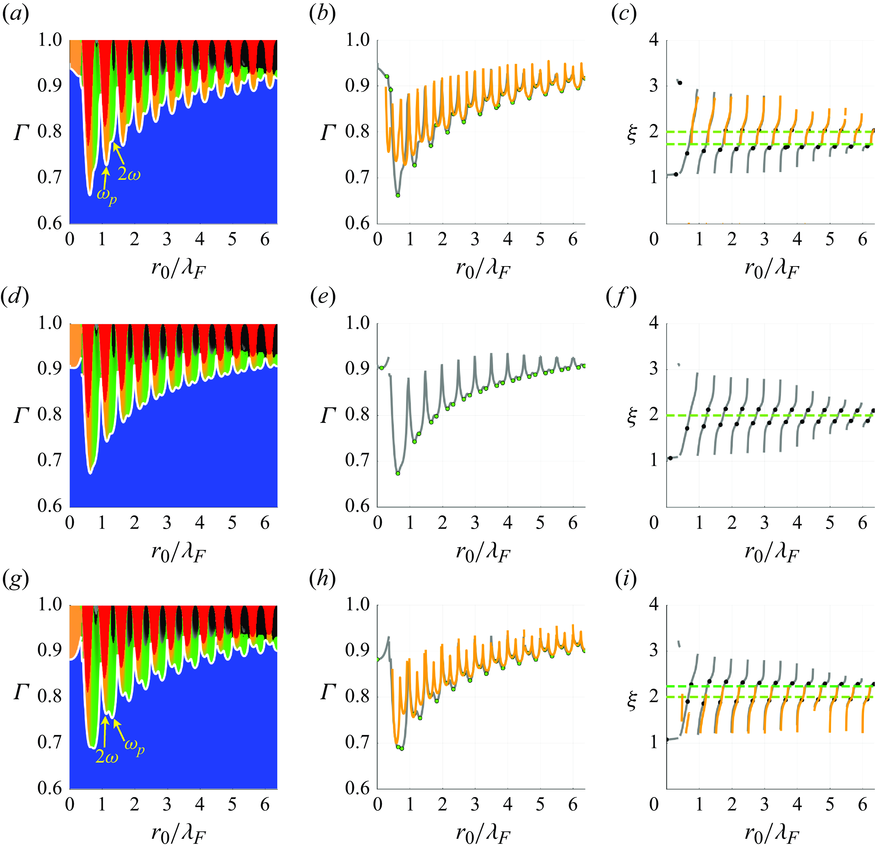
Figure 5. Orbital stability for walkers in convex potentials $(n \gt 0)$
for the experimental parameters specified in § 3. The force power,
$(n \gt 0)$
for the experimental parameters specified in § 3. The force power, $n$
, increases with successive rows, assuming values (a)–(c)
$n$
, increases with successive rows, assuming values (a)–(c) $n = 2$
, (d)–(f)
$n = 2$
, (d)–(f) $n = 3$
, and (g)–(i)
$n = 3$
, and (g)–(i) $n=4$
. (a,d,g) Orbital stability diagrams, with the stability of circular orbits indicated using the same colour scheme as in figure 3. (b,e,h) Critical memory of instability. Numerically computed stability boundaries (grey curves) may be compared with the asymptotic solutions (orange curves) defined in (4.2a
) and (4.4a
). Green dots represent the critical radii of instability, for which instabilities arise at lowest memory. (c,f,i) Dependence of the wobble number,
$n=4$
. (a,d,g) Orbital stability diagrams, with the stability of circular orbits indicated using the same colour scheme as in figure 3. (b,e,h) Critical memory of instability. Numerically computed stability boundaries (grey curves) may be compared with the asymptotic solutions (orange curves) defined in (4.2a
) and (4.4a
). Green dots represent the critical radii of instability, for which instabilities arise at lowest memory. (c,f,i) Dependence of the wobble number, $\xi = S/\omega$
, on the orbital radius along the stability boundary, as predicted by numerics (grey curves) and asymptotics (orange curves; see (4.2b
) and (4.4b
)). The black dots, which correspond to the critical radii of instability (green dots in panels b,e,h), lie close to the wobbling frequencies
$\xi = S/\omega$
, on the orbital radius along the stability boundary, as predicted by numerics (grey curves) and asymptotics (orange curves; see (4.2b
) and (4.4b
)). The black dots, which correspond to the critical radii of instability (green dots in panels b,e,h), lie close to the wobbling frequencies $2\omega$
and
$2\omega$
and $\omega _p = \sqrt {n+1}\omega$
(dashed horizontal lines). The wobble number (grey curves), increases monotonically with the orbital radius,
$\omega _p = \sqrt {n+1}\omega$
(dashed horizontal lines). The wobble number (grey curves), increases monotonically with the orbital radius, $r_0$
, then jumps downwards discontinuously at half-integer multiples of the Faraday wavelength.
$r_0$
, then jumps downwards discontinuously at half-integer multiples of the Faraday wavelength.
For convex power-law potentials of the form $V\!(r) \propto r^{n + 1}$
with
$V\!(r) \propto r^{n + 1}$
with $n \gt 0$
, of which the linear spring force (
$n \gt 0$
, of which the linear spring force ( $n = 1$
) is a special case,
$n = 1$
) is a special case, $2\omega$
- and
$2\omega$
- and $\omega _p$
-wobbling instabilities are prevalent, as is evident in figure 5 and table 3. The structural reconfiguration in the orbital stability diagram as
$\omega _p$
-wobbling instabilities are prevalent, as is evident in figure 5 and table 3. The structural reconfiguration in the orbital stability diagram as $n$
exceeds 3 reflects an interchange in the critical radii of instability for
$n$
exceeds 3 reflects an interchange in the critical radii of instability for $2\omega$
- and
$2\omega$
- and $\omega _p$
-wobbles. This interchange cannot be predicted by heuristic arguments based solely on consideration of the wave field, specifically the wave energy, zeros of Bessel functions (Labousse et al. Reference Labousse, Oza, Perrard and Bush2016) or the mean wave field (Liu et al. Reference Liu, Durey and Bush2023). Although the switch in instability mechanism at
$\omega _p$
-wobbles. This interchange cannot be predicted by heuristic arguments based solely on consideration of the wave field, specifically the wave energy, zeros of Bessel functions (Labousse et al. Reference Labousse, Oza, Perrard and Bush2016) or the mean wave field (Liu et al. Reference Liu, Durey and Bush2023). Although the switch in instability mechanism at $n = 3$
is predicted to be discrete in our asymptotic analysis (see table 3), the transition is continuous in the numerical results. Specifically, the instability tongues merge into a pair at
$n = 3$
is predicted to be discrete in our asymptotic analysis (see table 3), the transition is continuous in the numerical results. Specifically, the instability tongues merge into a pair at $n = 3$
(for which
$n = 3$
(for which $\omega _p = 2\omega$
) with the wobble number,
$\omega _p = 2\omega$
) with the wobble number, $\xi$
, being close to 2 along the stability boundary (see figure 5
d–f). Finally, we note that our asymptotic theory is not valid for
$\xi$
, being close to 2 along the stability boundary (see figure 5
d–f). Finally, we note that our asymptotic theory is not valid for $n = 3$
as the condition
$n = 3$
as the condition $\sin (\pi \sqrt {n+1}) \neq 0$
is violated, and thus a special asymptotic treatment would be required in this case.
$\sin (\pi \sqrt {n+1}) \neq 0$
is violated, and thus a special asymptotic treatment would be required in this case.
4.3.5. Conical potential
For a conical potential of the form $V\!(r) \propto r$
(corresponding to
$V\!(r) \propto r$
(corresponding to $n = 0$
), the attractive radial force is independent of radial position, namely
$n = 0$
), the attractive radial force is independent of radial position, namely $\boldsymbol{F}\cdot \boldsymbol{n} = -k$
. This situation is thus similar to that of a Coriolis force, for which
$\boldsymbol{F}\cdot \boldsymbol{n} = -k$
. This situation is thus similar to that of a Coriolis force, for which $\boldsymbol{F}\cdot \boldsymbol{n} = 2m\Omega r_0\omega \approx -2m |\Omega | u_0$
for inertial orbits. Indeed, the stability boundary for the conical potential is indistinguishable from that of the Coriolis force for
$\boldsymbol{F}\cdot \boldsymbol{n} = 2m\Omega r_0\omega \approx -2m |\Omega | u_0$
for inertial orbits. Indeed, the stability boundary for the conical potential is indistinguishable from that of the Coriolis force for $r_0/\lambda _F \gtrsim 0.5$
(see figure 6), with equivalent asymptotic stability boundaries (as may be seen by comparing (4.1a
) and (4.1b
) respectively to (4.2a
) with
$r_0/\lambda _F \gtrsim 0.5$
(see figure 6), with equivalent asymptotic stability boundaries (as may be seen by comparing (4.1a
) and (4.1b
) respectively to (4.2a
) with $N = 0$
and
$N = 0$
and $N = 1$
). Nevertheless, there are two main differences. First, small-radius orbits (
$N = 1$
). Nevertheless, there are two main differences. First, small-radius orbits ( $r_0/\lambda _F \lesssim 0.25$
) are unstable for a conical potential (see Appendix E), yet are stable for a Coriolis force (Oza Reference Oza2014). Second, the
$r_0/\lambda _F \lesssim 0.25$
) are unstable for a conical potential (see Appendix E), yet are stable for a Coriolis force (Oza Reference Oza2014). Second, the $O(1/k_F r_0)$
detuning from resonant 2-wobbles persists for a conical potential (see 4.2b
), but not for the Coriolis force (see 4.1c
). Finally, we note that potential-driven wobbling with frequency
$O(1/k_F r_0)$
detuning from resonant 2-wobbles persists for a conical potential (see 4.2b
), but not for the Coriolis force (see 4.1c
). Finally, we note that potential-driven wobbling with frequency $\omega _p = \omega$
is suppressed in the conical potential.
$\omega _p = \omega$
is suppressed in the conical potential.
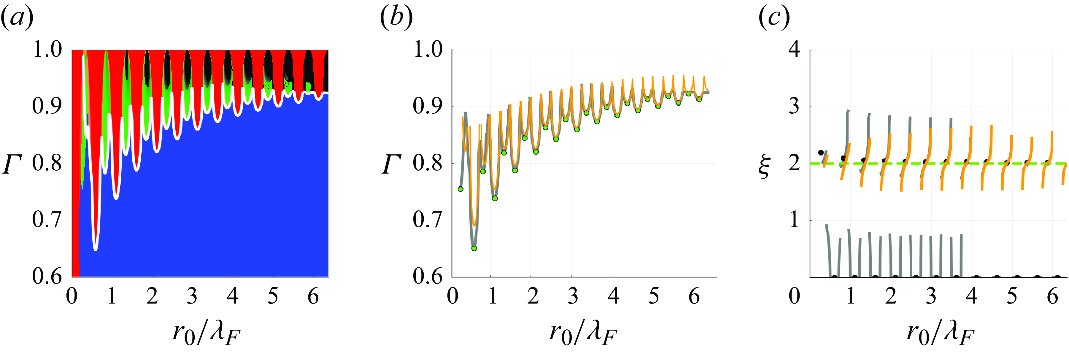
Figure 6. Orbital stability for walkers in a conical potential, equivalently a radially uniform central force, $\boldsymbol{F} = -k\boldsymbol{x\!}_p/|\boldsymbol{x\!}_p|$
, for the experimental parameters specified in § 3. (a) Stability diagram, with the same colour scheme as in figure 3. The white curve denotes the stability boundary for the Coriolis system (see figure 3
c). The strong agreement between the instability boundaries in the two systems is a consequence of the constancy of the Coriolis force for constant-speed motion. (b) Comparison between the numerically computed stability boundary (grey curve) and the asymptotic solutions (orange curves) defined using (4.2a
). (c) Numerically computed (grey) and analytic solutions (orange, see 4.2b
) for the wobble number,
$\boldsymbol{F} = -k\boldsymbol{x\!}_p/|\boldsymbol{x\!}_p|$
, for the experimental parameters specified in § 3. (a) Stability diagram, with the same colour scheme as in figure 3. The white curve denotes the stability boundary for the Coriolis system (see figure 3
c). The strong agreement between the instability boundaries in the two systems is a consequence of the constancy of the Coriolis force for constant-speed motion. (b) Comparison between the numerically computed stability boundary (grey curve) and the asymptotic solutions (orange curves) defined using (4.2a
). (c) Numerically computed (grey) and analytic solutions (orange, see 4.2b
) for the wobble number, $\xi = S/\omega$
, along the stability boundary, for
$\xi = S/\omega$
, along the stability boundary, for $\xi \lt 4$
. The black dots denote the critical memory of instability, corresponding to the green dots in (b).
$\xi \lt 4$
. The black dots denote the critical memory of instability, corresponding to the green dots in (b).
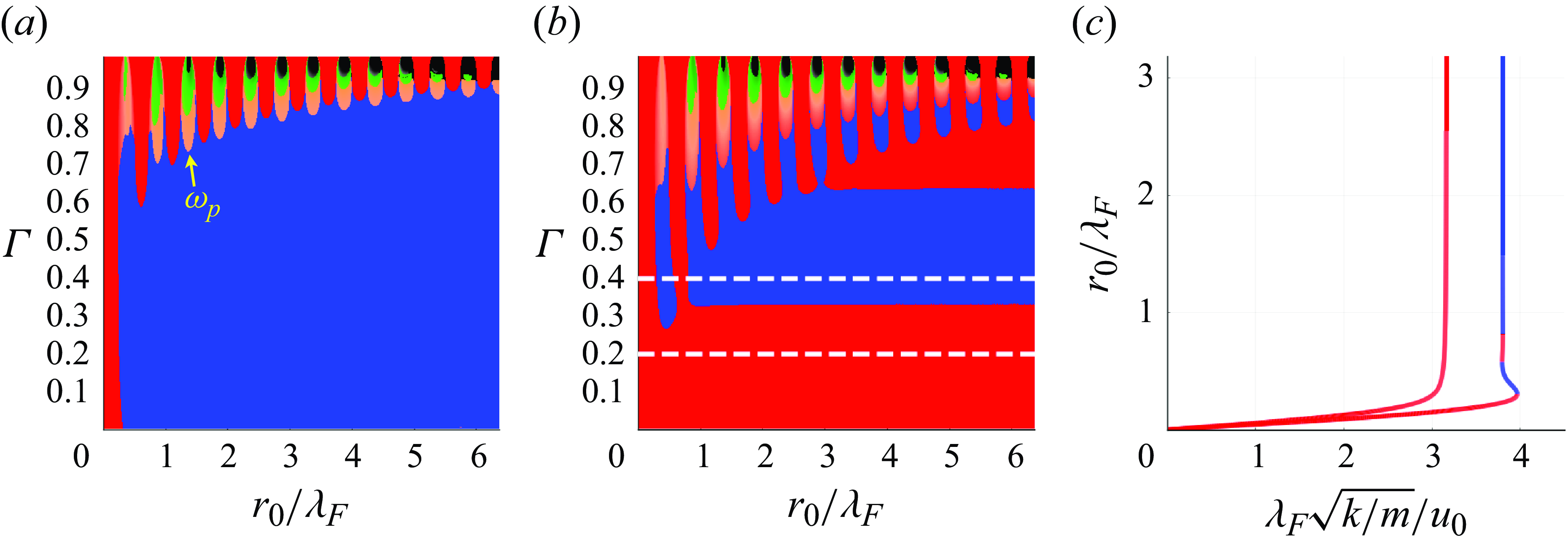
Figure 7. Orbital stability for walkers in concave potentials ( $V\!(r) \propto r^{n+1}$
for
$V\!(r) \propto r^{n+1}$
for $-1 \lt n \lt 0$
or
$-1 \lt n \lt 0$
or $V\!(r) \propto \ln r$
for
$V\!(r) \propto \ln r$
for $n = -1$
) for the experimental parameters specified in § 3, with the same colour scheme as in figure 3. (a) Stability diagram for
$n = -1$
) for the experimental parameters specified in § 3, with the same colour scheme as in figure 3. (a) Stability diagram for $n = -0.5$
. The potential-driven instability (light red) arises at a lower memory than the
$n = -0.5$
. The potential-driven instability (light red) arises at a lower memory than the $2\omega$
-wobbles (green); see table 3. (b) Stability diagram for a logarithmic potential. Monotonic instabilities represent the dominant instability mechanism, as the potential-driven instability occurs at a frequency
$2\omega$
-wobbles (green); see table 3. (b) Stability diagram for a logarithmic potential. Monotonic instabilities represent the dominant instability mechanism, as the potential-driven instability occurs at a frequency $\omega _p = \sqrt {n+1}\omega = 0$
for
$\omega _p = \sqrt {n+1}\omega = 0$
for $n = -1$
. (c) Dependence of the orbital radius on the central force constant,
$n = -1$
. (c) Dependence of the orbital radius on the central force constant, $k$
, for
$k$
, for $n = -1$
, with
$n = -1$
, with $\Gamma = 0.2$
and
$\Gamma = 0.2$
and $\Gamma = 0.4$
corresponding to the dashed lines in panel (b). We note that portions of the orbital solution curve with positive slope are unstable with monotonically growing perturbations, in accordance with Theorem1.
$\Gamma = 0.4$
corresponding to the dashed lines in panel (b). We note that portions of the orbital solution curve with positive slope are unstable with monotonically growing perturbations, in accordance with Theorem1.
4.3.6. Concave potentials
For concave potentials with power-law form $V\!(r)\propto r^{n+1}$
for
$V\!(r)\propto r^{n+1}$
for $-1 \lt n \lt 0$
, perturbations either grow monotonically or are
$-1 \lt n \lt 0$
, perturbations either grow monotonically or are $\omega _p$
-wobbles (see figure 7
a), in agreement with our asymptotic predictions (see table 3). However, for the logarithmic potential,
$\omega _p$
-wobbles (see figure 7
a), in agreement with our asymptotic predictions (see table 3). However, for the logarithmic potential, $V\!(r) \propto \ln (r)$
(corresponding to
$V\!(r) \propto \ln (r)$
(corresponding to $n = -1$
), there is a qualitative change in the structure of the stability diagram in figure 7(b). Specifically, monotonic instabilities dominate (in accordance with
$n = -1$
), there is a qualitative change in the structure of the stability diagram in figure 7(b). Specifically, monotonic instabilities dominate (in accordance with $\omega _p = 0$
), plateaus in the stability boundary emerge at
$\omega _p = 0$
), plateaus in the stability boundary emerge at $\Gamma \approx 0.35$
and
$\Gamma \approx 0.35$
and $\Gamma \approx 0.65$
(associated with changes in slope of the orbital solution curve; see figure 7
c), and the monotonic instability tongues resemble tear drops, which widen and merge at larger radius, resulting in islands of stability at high memory. As memory is further increased, these stability islands are terminated by an oscillatory instability, whose frequency is neither commensurate with the orbital frequency nor equal to the potential-driven instability frequency,
$\Gamma \approx 0.65$
(associated with changes in slope of the orbital solution curve; see figure 7
c), and the monotonic instability tongues resemble tear drops, which widen and merge at larger radius, resulting in islands of stability at high memory. As memory is further increased, these stability islands are terminated by an oscillatory instability, whose frequency is neither commensurate with the orbital frequency nor equal to the potential-driven instability frequency, $\omega _p = 0$
(Tambasco et al. Reference Tambasco, Harris, Oza, Rosales and Bush2016). As these anomalous features violate the scaling of
$\omega _p = 0$
(Tambasco et al. Reference Tambasco, Harris, Oza, Rosales and Bush2016). As these anomalous features violate the scaling of $\beta = O(\ln \hat {r}_0)$
leveraged in Appendix D, a new asymptotic framework to capture them will be left for future work. In particular, the tear-drop-shaped instability boundaries cannot be uniquely defined in terms of the orbital radius, thus precluding the development of explicit formulae for the critical memory.
$\beta = O(\ln \hat {r}_0)$
leveraged in Appendix D, a new asymptotic framework to capture them will be left for future work. In particular, the tear-drop-shaped instability boundaries cannot be uniquely defined in terms of the orbital radius, thus precluding the development of explicit formulae for the critical memory.
5. Discussion
Orbital pilot-wave dynamics has provided one of the central paradigms for the emergence of quantisation and quantum-like statistics from classical pilot-wave dynamics (Bush & Oza Reference Bush and Oza2020). The particle is able to access only a discrete number of orbitals owing to the dynamic constraint imposed on it by its quasi-monochromatic pilot-wave field (Fort et al. Reference Fort, Eddi, Moukhtar, Boudaoud and Couder2010). At high memory, the droplet switches intermittently between unstable periodic orbits (Harris & Bush Reference Harris and Bush2014; Perrard et al. Reference Perrard, Labousse, Fort and Couder2014a ,Reference Perrard, Labousse, Miskin, Fort and Couder b ; Oza et al. Reference Oza, Wind-Willassen, Harris, Rosales and Bush2014b ). This physical picture suggests that the superposition of statistical states in quantum systems may be rooted in an underlying, but currently unresolved, chaotic pilot-wave dynamics, a perspective forwarded by Gutzwiller in his periodic orbit theory (Müller et al. Reference Müller, Heusler, Braun, Haake and Altland2005). Our analysis of orbital stability provides a step towards assessing the relative propensity of different orbital states in chaotic pilot-wave dynamics.
For droplets executing inertial orbits in a rotating frame, the onset of instability arises from a resonance between the orbital frequency, $\omega$
, and the destabilisation frequency,
$\omega$
, and the destabilisation frequency, $S$
, and is characterised by either monotonically growing perturbations (
$S$
, and is characterised by either monotonically growing perturbations ( $S = 0$
) or 2-wobbles (
$S = 0$
) or 2-wobbles ( $S = 2\omega$
). For droplets executing circular orbits under the influence of an axisymmetric potential, we have demonstrated that the natural frequency of radial oscillation is
$S = 2\omega$
). For droplets executing circular orbits under the influence of an axisymmetric potential, we have demonstrated that the natural frequency of radial oscillation is $\omega _p$
(see (2.5)), resulting in potential-driven instabilities at frequency
$\omega _p$
(see (2.5)), resulting in potential-driven instabilities at frequency $S = \omega _p$
, in addition to monotonic and
$S = \omega _p$
, in addition to monotonic and $2\omega$
-instabilities. The difference between
$2\omega$
-instabilities. The difference between $\omega _p$
and its analogue in classical orbital mechanics (
$\omega _p$
and its analogue in classical orbital mechanics ( $\omega _c$
, see (2.3)) arises because the system acts to conserve orbital speed rather than angular momentum. Equation (2.5) indicates that in radial potentials,
$\omega _c$
, see (2.3)) arises because the system acts to conserve orbital speed rather than angular momentum. Equation (2.5) indicates that in radial potentials, $V\!(r) \propto r^q$
, for which
$V\!(r) \propto r^q$
, for which $\omega _p = \sqrt {q}\omega$
, stable circular orbits can arise in our system only if
$\omega _p = \sqrt {q}\omega$
, stable circular orbits can arise in our system only if $q \gt 0$
. In this case, the near-critical oscillatory modes of frequency
$q \gt 0$
. In this case, the near-critical oscillatory modes of frequency $\omega _p$
are resonant if and only if
$\omega _p$
are resonant if and only if $q$
is a perfect square.
$q$
is a perfect square.
To characterise the emergence of wave-driven and potential-driven instabilities in different settings, we generalised our analysis to consider the confinement of a walking droplet by a power-law central force of the form $\boldsymbol{F} = -k |\boldsymbol{x\!}_p|^{n-1}\boldsymbol{x\!}_p$
with
$\boldsymbol{F} = -k |\boldsymbol{x\!}_p|^{n-1}\boldsymbol{x\!}_p$
with $n \geqslant -1$
, for which
$n \geqslant -1$
, for which $\omega _p = \omega \sqrt {n+1}$
. When the central force increases with radial distance (
$\omega _p = \omega \sqrt {n+1}$
. When the central force increases with radial distance ( $n \gt 0$
), as is the case for a harmonic potential (
$n \gt 0$
), as is the case for a harmonic potential ( $n = 1$
), wave-driven and potential-driven wobbling instabilities are prevalent. The instability tongues in the stability diagram alternate between
$n = 1$
), wave-driven and potential-driven wobbling instabilities are prevalent. The instability tongues in the stability diagram alternate between $2\omega$
-wobbles and
$2\omega$
-wobbles and $\omega _p$
-wobbles every half wavelength with increasing orbital radius. Of particular interest is the case
$\omega _p$
-wobbles every half wavelength with increasing orbital radius. Of particular interest is the case $n = 3$
, for which the potential-driven instabilities are resonant with
$n = 3$
, for which the potential-driven instabilities are resonant with $\omega _p = 2\omega$
, leading to merging pairs of
$\omega _p = 2\omega$
, leading to merging pairs of $2\omega$
and
$2\omega$
and $\omega _p$
instability tongues. In this case, numerical simulations reveal that 2-wobbles are prevalent in the weakly unstable regime. When the spring force is radially uniform (
$\omega _p$
instability tongues. In this case, numerical simulations reveal that 2-wobbles are prevalent in the weakly unstable regime. When the spring force is radially uniform ( $n = 0$
), the stability diagram is similar in structure to that of the Coriolis force, consisting of alternating monotonic and
$n = 0$
), the stability diagram is similar in structure to that of the Coriolis force, consisting of alternating monotonic and $2\omega$
-wobble instability tongues. Indeed, the asymptotic stability boundaries are precisely equal for the two systems. Finally, when the spring force decreases with radial distance (
$2\omega$
-wobble instability tongues. Indeed, the asymptotic stability boundaries are precisely equal for the two systems. Finally, when the spring force decreases with radial distance ( $-1 \leqslant n \lt 0$
), monotonic instabilities are prevalent, particularly in the case of a logarithmic potential (
$-1 \leqslant n \lt 0$
), monotonic instabilities are prevalent, particularly in the case of a logarithmic potential ( $n = -1$
), for which
$n = -1$
), for which $\omega _p = 0$
.
$\omega _p = 0$
.
Our study also highlights the limitations of rationalising the onset of instability in terms of simple heuristic arguments (Labousse et al. Reference Labousse, Oza, Perrard and Bush2016; Liu et al. Reference Liu, Durey and Bush2023). Specifically, our asymptotic and numerical investigations in § 4 demonstrated that the critical radii of the $2\omega$
and
$2\omega$
and $\omega _p$
instability tongues can alternate between being close to
$\omega _p$
instability tongues can alternate between being close to $\sin (2k_F r_0) = 1$
or
$\sin (2k_F r_0) = 1$
or $\sin (2k_F r_0) = -1$
, depending on the power-law force,
$\sin (2k_F r_0) = -1$
, depending on the power-law force, $n$
(see table 3). As such, one cannot simply rationalise the critical radii at the onset of 2-wobbles in terms of the zeros of Bessel functions (Labousse et al. Reference Labousse, Oza, Perrard and Bush2016), the minima of the wave energy (Liu et al. Reference Liu, Durey and Bush2023), or the curvature of the mean wave field (Liu et al. Reference Liu, Durey and Bush2023), all of which are independent of the confining force. Likewise, these heuristic arguments can neither distinguish between
$n$
(see table 3). As such, one cannot simply rationalise the critical radii at the onset of 2-wobbles in terms of the zeros of Bessel functions (Labousse et al. Reference Labousse, Oza, Perrard and Bush2016), the minima of the wave energy (Liu et al. Reference Liu, Durey and Bush2023), or the curvature of the mean wave field (Liu et al. Reference Liu, Durey and Bush2023), all of which are independent of the confining force. Likewise, these heuristic arguments can neither distinguish between $2\omega$
and
$2\omega$
and $\omega _p$
wobbling instabilities, nor assess their relative likelihood as a function of memory. Instead, we find that the relative ordering of the
$\omega _p$
wobbling instabilities, nor assess their relative likelihood as a function of memory. Instead, we find that the relative ordering of the $2\omega$
and
$2\omega$
and $\omega _p$
instability tongues is related to the observation that the wobble number,
$\omega _p$
instability tongues is related to the observation that the wobble number, $\xi = S/\omega$
, increases monotonically across pairs of wobbling instability tongues, with downward jumps arising when the orbital radius is close to a half-integer multiple of the Faraday wavelength (see figure 5). Rationalising this observation remains the subject of ongoing investigation.
$\xi = S/\omega$
, increases monotonically across pairs of wobbling instability tongues, with downward jumps arising when the orbital radius is close to a half-integer multiple of the Faraday wavelength (see figure 5). Rationalising this observation remains the subject of ongoing investigation.
As part of our analysis, we have developed Theorem1 (see Appendix B), which provides a simple diagnostic for the onset of monotonic instabilities in a central or Coriolis force in terms of the slope of the orbital solution curve (see figure 3 a,b and figure 7 c). Specifically, if the confining potential decays too rapidly in space to rein in outward perturbations, then the perturbations grow monotonically in time and the circular orbit destabilises. Consequently, monotonic instabilities are more prevalent in concave potentials than convex potentials (see § 4). We have also used this result to justify the instability of small circular orbits for sub-linear central forces (see Appendix E). We note that this result is an extension of Theorem 1 of Oza et al. (Reference Oza, Harris, Rosales and Bush2014a ) for orbital pilot-wave dynamics in a Coriolis force. However, our proof does not rely explicitly on the particular properties of the stroboscopic pilot-wave system, and so may be applied more generally, to any classical particle orbiting in an axisymmetric potential or a Coriolis force field.
It is also worth considering the stability of walkers in an oscillatory potential of the form $V\!(r) \propto \textrm{J}_0(k_F r)$
, as was explored experimentally and numerically by Tambasco & Bush (Reference Tambasco and Bush2018). By using Bessel’s equation to evaluate
$V\!(r) \propto \textrm{J}_0(k_F r)$
, as was explored experimentally and numerically by Tambasco & Bush (Reference Tambasco and Bush2018). By using Bessel’s equation to evaluate $V''(r_0)$
in (2.5), we compute
$V''(r_0)$
in (2.5), we compute $\omega _p = \omega \sqrt {r_0 k_F \textrm{J}_0(k_F r_0)/\textrm{J}_1(k_F r_0)}$
, which corresponds to potential-driven wobbling when the argument of the square root is positive, and monotonic growth otherwise. When the orbital radius is such that
$\omega _p = \omega \sqrt {r_0 k_F \textrm{J}_0(k_F r_0)/\textrm{J}_1(k_F r_0)}$
, which corresponds to potential-driven wobbling when the argument of the square root is positive, and monotonic growth otherwise. When the orbital radius is such that $\textrm{J}_0(k_F r_0)$
and
$\textrm{J}_0(k_F r_0)$
and $\textrm{J}_1(k_F r_0)$
are of the same sign, radial perturbations oscillate in time, with the oscillation frequency increasing with proximity to the zeros of
$\textrm{J}_1(k_F r_0)$
are of the same sign, radial perturbations oscillate in time, with the oscillation frequency increasing with proximity to the zeros of $\textrm{J}_1(k_F r_0)$
. However, when the signs of
$\textrm{J}_1(k_F r_0)$
. However, when the signs of $\textrm{J}_0(k_F r_0)$
and
$\textrm{J}_0(k_F r_0)$
and $\textrm{J}_1(k_F r_0)$
differ, radial perturbations grow exponentially in time, giving rise to instability. Our theoretical treatment of walkers as constant-speed particles (see § 2.2) thus predicts that circular orbits are stable only within narrow radial intervals separated approximately by half the Faraday wavelength, in accordance with the experimental observations of Tambasco & Bush (Reference Tambasco and Bush2018). Such a case is particularly interesting given that the mean pilot wave of a droplet executing a circular orbit takes a comparable form in the high-memory limit (Tambasco & Bush Reference Tambasco and Bush2018), so one can then consider the stability of an orbiting droplet in its self-potential.
$\textrm{J}_1(k_F r_0)$
differ, radial perturbations grow exponentially in time, giving rise to instability. Our theoretical treatment of walkers as constant-speed particles (see § 2.2) thus predicts that circular orbits are stable only within narrow radial intervals separated approximately by half the Faraday wavelength, in accordance with the experimental observations of Tambasco & Bush (Reference Tambasco and Bush2018). Such a case is particularly interesting given that the mean pilot wave of a droplet executing a circular orbit takes a comparable form in the high-memory limit (Tambasco & Bush Reference Tambasco and Bush2018), so one can then consider the stability of an orbiting droplet in its self-potential.
Finally, our analysis has considered a single point in parameter space in the generalised pilot-wave framework (Durey & Bush Reference Durey and Bush2021), corresponding to the experimental parameters used by Harris & Bush (Reference Harris and Bush2014). For example, in § 4.3, we have assumed that the dimensionless mass number satisfies $4M \gt 1$
, as is the case in the laboratory. Our theoretical formalism allows for a broader exploration of orbital pilot-wave dynamics at a much wider range of parameter values, which will be the subject of future work. Of particular interest will be the small
$4M \gt 1$
, as is the case in the laboratory. Our theoretical formalism allows for a broader exploration of orbital pilot-wave dynamics at a much wider range of parameter values, which will be the subject of future work. Of particular interest will be the small $M$
, long-memory limit, where quantum effects are known to be most prevalent (Oza et al. Reference Oza, Rosales and Bush2018). In this long-memory limit, the instantaneous pilot-wave form converges to the mean (Durey, Milewski & Bush Reference Durey, Milewski and Bush2018), so one expects the self-potential associated with the mean pilot-wave form to play a role equivalent to the applied potential in the orbital stability. This physical picture, which evokes the role of the quantum potential in Bohmian mechanics (Holland Reference Holland1995), will be explored in an upcoming manuscript.
$M$
, long-memory limit, where quantum effects are known to be most prevalent (Oza et al. Reference Oza, Rosales and Bush2018). In this long-memory limit, the instantaneous pilot-wave form converges to the mean (Durey, Milewski & Bush Reference Durey, Milewski and Bush2018), so one expects the self-potential associated with the mean pilot-wave form to play a role equivalent to the applied potential in the orbital stability. This physical picture, which evokes the role of the quantum potential in Bohmian mechanics (Holland Reference Holland1995), will be explored in an upcoming manuscript.
Funding
J.B. gratefully acknowledges the generous financial support of the NSF through grant CMMI-2154151 and the Office of Naval Research through grant N000014-24-1-2232.
Declaration of interests
The authors report no conflict of interest.
Author contributions
J.B. and M.D. conceived the project. N.L. was responsible for the mathematical and numerical developments, which were overseen by M.D. All authors contributed to the writing.
Data availability statement
The data that support the findings of this study are available from the corresponding authors, M.D. and J.B., upon reasonable request.
Appendix A. Orbital stability at low orbital memory
The regime of low orbital memory, $M_e^O \ll 1$
, in which the droplet’s horizontal velocity evolves slowly relative to the memory time,
$M_e^O \ll 1$
, in which the droplet’s horizontal velocity evolves slowly relative to the memory time, $T_M$
, emerges for relatively large orbits or weak vibrational forcing. In this weak-acceleration limit, one may substitute the approximation
$T_M$
, emerges for relatively large orbits or weak vibrational forcing. In this weak-acceleration limit, one may substitute the approximation $\boldsymbol{x\!}_p(t) - \boldsymbol{x\!}_p(s) \approx (t-s)\,\dot {\!\boldsymbol{x}\!}_p(t) - ({1}/{2})(t-s)^2\,\ddot {\!\boldsymbol{x}\!}_p(t)$
into the wave force integral term in (3.2) and evaluate the resulting integrals (Bush et al. Reference Bush, Oza and Moláček2014). The droplet’s trajectory equation may thus be approximated by the local form
$\boldsymbol{x\!}_p(t) - \boldsymbol{x\!}_p(s) \approx (t-s)\,\dot {\!\boldsymbol{x}\!}_p(t) - ({1}/{2})(t-s)^2\,\ddot {\!\boldsymbol{x}\!}_p(t)$
into the wave force integral term in (3.2) and evaluate the resulting integrals (Bush et al. Reference Bush, Oza and Moláček2014). The droplet’s trajectory equation may thus be approximated by the local form
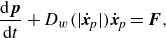 \begin{equation} \frac {\textrm{d} {\boldsymbol{p}}}{\textrm{d}{t}} + D_w(|\,\dot {\!\boldsymbol{x}\!}_p|)\,\dot {\!\boldsymbol{x}\!}_p = \boldsymbol{F}, \end{equation}
where $\boldsymbol{p} = m\gamma _B(|\,\dot {\!\boldsymbol{x}\!}_p|)\,\dot {\!\boldsymbol{x}\!}_p$
is the droplet’s effective momentum, expressed in terms of the wave-induced added mass, or ‘hydrodynamic boost factor’,
$\boldsymbol{p} = m\gamma _B(|\,\dot {\!\boldsymbol{x}\!}_p|)\,\dot {\!\boldsymbol{x}\!}_p$
is the droplet’s effective momentum, expressed in terms of the wave-induced added mass, or ‘hydrodynamic boost factor’,
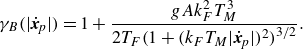 \begin{equation} \gamma _B(|\,\dot {\!\boldsymbol{x}\!}_p|) = 1 + \frac {gAk_F^2 T_M^3}{2T_F\big (1 + (k_F T_M|\,\dot {\!\boldsymbol{x}\!}_p|)^2\big )^{3/2}}. \end{equation}
The wave force also gives rise to a speed-dependent drag coefficient,
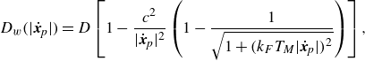 \begin{equation} D_w(|\,\dot {\!\boldsymbol{x}\!}_p|) = D\left [1 - \frac {c^2}{|\,\dot {\!\boldsymbol{x}\!}_p|^2}\left (1 - \frac {1}{\sqrt {1 + (k_F T_M|\,\dot {\!\boldsymbol{x}\!}_p|)^2}}\right )\right ], \end{equation}
that drives the droplet towards the steady walking speed, $u_0$
(Bush et al. Reference Bush, Oza and Moláček2014). Specifically, the walking speed satisfies
$u_0$
(Bush et al. Reference Bush, Oza and Moláček2014). Specifically, the walking speed satisfies $D_w(u_0) = 0$
, with
$D_w(u_0) = 0$
, with $D_w \gt 0$
if
$D_w \gt 0$
if $|\,\dot {\!\boldsymbol{x}\!}_p| \gt u_0$
and
$|\,\dot {\!\boldsymbol{x}\!}_p| \gt u_0$
and $D_w \lt 0$
otherwise.
$D_w \lt 0$
otherwise.
Following the analysis of Bush et al. (Reference Bush, Oza and Moláček2014) for steady circular orbits with radius $r_0$
and frequency
$r_0$
and frequency $\omega \gt 0$
, the orbital speed,
$\omega \gt 0$
, the orbital speed, $U = r_0\omega$
, is equal to the free-walking speed,
$U = r_0\omega$
, is equal to the free-walking speed, $u_0$
. The orbital radius satisfies
$u_0$
. The orbital radius satisfies $r_0 V'(r_0) = p(u_0) u_0$
for orbiting in a potential with force
$r_0 V'(r_0) = p(u_0) u_0$
for orbiting in a potential with force $\boldsymbol{F} = -\boldsymbol \nabla V(|\boldsymbol{x\!}_p|)$
, and is defined as
$\boldsymbol{F} = -\boldsymbol \nabla V(|\boldsymbol{x\!}_p|)$
, and is defined as $r_0 = p(u_0)/(2m |\Omega |)$
for orbiting in response to a Coriolis force,
$r_0 = p(u_0)/(2m |\Omega |)$
for orbiting in response to a Coriolis force, $\boldsymbol{F} = -2m \boldsymbol{\Omega }\times \,\dot {\!\boldsymbol{x}\!}_p$
, where
$\boldsymbol{F} = -2m \boldsymbol{\Omega }\times \,\dot {\!\boldsymbol{x}\!}_p$
, where $p(u) = m\gamma _B(u)u$
. The orbital stability may be determined by defining the droplet’s position and velocity as
$p(u) = m\gamma _B(u)u$
. The orbital stability may be determined by defining the droplet’s position and velocity as
 \begin{align} \boldsymbol{x\!}_p(t) = r(t)(\cos \theta (t),\sin \theta (t)) \quad \mbox{and}\quad \,\dot {\!\boldsymbol{x}\!}_p(t) = u(t)(-\sin \phi (t),\cos \phi (t)), \end{align}
respectively. For small perturbations, we express the radius and speed as $r(t) = r_0 + \epsilon r_1(t)$
and
$r(t) = r_0 + \epsilon r_1(t)$
and $u(t) = u_0 + \epsilon u_1(t)$
, where
$u(t) = u_0 + \epsilon u_1(t)$
, where $0 \lt \epsilon \ll 1$
, and likewise perturb the polar angles
$0 \lt \epsilon \ll 1$
, and likewise perturb the polar angles $\theta$
and
$\theta$
and $\phi$
. We then substitute this perturbation ansatz into (A1a
) and use Taylor expansions to derive linear equations for the perturbed variables. Eliminating the perturbed polar angles yields a pair of coupled evolution equations for the perturbed radius and speed, as summarised as follows.
$\phi$
. We then substitute this perturbation ansatz into (A1a
) and use Taylor expansions to derive linear equations for the perturbed variables. Eliminating the perturbed polar angles yields a pair of coupled evolution equations for the perturbed radius and speed, as summarised as follows.
A.1. Walking in a rotating frame
When the droplet motion is subjected to a Coriolis force, the radial and speed perturbations evolve according to
 \begin{equation} \ddot r_1 + \omega ^2 r_1 = \omega \left (\frac {u_0 p'(u_0)}{p(u_0)}\right ) u_1 \quad \mbox{and}\quad p'(u_0) \dot u_1 + u_0 D_w'(u_0)u_1 = 0. \end{equation}
The eigenvalues $s_\pm = \pm \textrm{i} \omega$
reflect the translational invariance of the orbit and
$s_\pm = \pm \textrm{i} \omega$
reflect the translational invariance of the orbit and $s_0 = -u_0 D_w'(u_0)/p'(u_0)$
corresponds to decaying speed perturbations when
$s_0 = -u_0 D_w'(u_0)/p'(u_0)$
corresponds to decaying speed perturbations when $p'(u_0) \gt 0$
. Circular orbits in a rotating frame are thus stable at low orbital memory.
$p'(u_0) \gt 0$
. Circular orbits in a rotating frame are thus stable at low orbital memory.
A.2. Walking in a central force
For a droplet confined to an axisymmetric potential, perturbations evolve according to
 \begin{equation} \ddot r_1 + \omega _p^2 r_1 = \omega \left (1 + \frac {u_0 p'(u_0)}{p(u_0)}\right ) u_1 \quad \mbox{and}\quad p'(u_0) \dot u_1 + u_0 D_w'(u_0)u_1 = - \frac {p(u_0)}{r_0}\dot {r}_1, \end{equation}
where the natural frequency of radial perturbation, $\omega _p = \omega \sqrt {1 + r_0 V''(r_0)/V'(r_0)}$
, is identical to the potential-driven wobbling frequency derived in § 2.2 for constant-speed particles. In the large-radius limit, the eigenvalues of (A4) are
$\omega _p = \omega \sqrt {1 + r_0 V''(r_0)/V'(r_0)}$
, is identical to the potential-driven wobbling frequency derived in § 2.2 for constant-speed particles. In the large-radius limit, the eigenvalues of (A4) are $s_0 = -u_0 D_w'(u_0)/p'(u_0) + O (r_0^{-2} )$
and
$s_0 = -u_0 D_w'(u_0)/p'(u_0) + O (r_0^{-2} )$
and
 \begin{align} s_{\pm } = \pm \textrm{i}\omega _p - \frac {u_0\big (p(u_0) + u_0p'(u_0)\big )}{2r_0^2\Big(u_0^2 D_w'(u_0)^2 + \omega _p^2 p'(u_0)^2\Big)}\left (u_0 D_w'(u_0) \pm \textrm{i} \omega _p p'(u_0)\right ) + O\Big(r_0^{-4}\Big), \end{align}
where $s_0$
is related to the decay of speed perturbations (as in the case of a Coriolis force) and
$s_0$
is related to the decay of speed perturbations (as in the case of a Coriolis force) and $s_\pm$
reflect the natural frequency of radial oscillations. As
$s_\pm$
reflect the natural frequency of radial oscillations. As $p(u_0) + u_0p'(u_0) \gt 0$
in the regime that walking droplets may be observed in the laboratory (Turton Reference Turton2020), we conclude that the real part of
$p(u_0) + u_0p'(u_0) \gt 0$
in the regime that walking droplets may be observed in the laboratory (Turton Reference Turton2020), we conclude that the real part of $s_\pm$
is negative, albeit close to zero. Consequently, we deduce that
$s_\pm$
is negative, albeit close to zero. Consequently, we deduce that $s_\pm$
form a pair of near-critical stable eigenvalues in the weak-acceleration limit. Finally, we note that as
$s_\pm$
form a pair of near-critical stable eigenvalues in the weak-acceleration limit. Finally, we note that as $\omega _p$
does not depend explicitly on the wave-induced added mass,
$\omega _p$
does not depend explicitly on the wave-induced added mass, $\gamma _B$
, for a fixed orbital radius, our analysis incorporates the Rayleigh oscillator model (Labousse & Perrard Reference Labousse and Perrard2014) as a special case, for which
$\gamma _B$
, for a fixed orbital radius, our analysis incorporates the Rayleigh oscillator model (Labousse & Perrard Reference Labousse and Perrard2014) as a special case, for which $\gamma _B = 1$
and
$\gamma _B = 1$
and $D_w(u) = D_0(u^2/u_0^2 - 1)$
.
$D_w(u) = D_0(u^2/u_0^2 - 1)$
.
Appendix B. Orbital stability framework
To investigate the stability of circular orbits in the hydrodynamic pilot-wave system, we recast the trajectory equation (3.2) into polar coordinates, namely
 \begin{gather} \boldsymbol{x\!}_p(t) = r(t)(\cos \theta (t),\sin \theta (t)), \end{gather}
and perturb the droplet motion from a circular orbit at time $t = 0$
(Oza et al. Reference Oza, Harris, Rosales and Bush2014a
). The radial (
$t = 0$
(Oza et al. Reference Oza, Harris, Rosales and Bush2014a
). The radial ( $l = r$
) and tangential (
$l = r$
) and tangential ( $l = \theta$
) force balances thus take the form
$l = \theta$
) force balances thus take the form
 \begin{gather} f_l(r,\dot {r},\ddot {r},\dot {\theta },\ddot {\theta }) + \zeta f_{{ext},l}(r,\dot {r},\dot {\theta }) + \int _{-\infty }^t w_l(r(t),r(s),\theta (t)-\theta (s),t-s){\,\textrm{d}s} = \epsilon C_l\delta (t), \end{gather}
where
 \begin{equation} f_r(r,\dot {r},\ddot {r},\dot {\theta },\ddot {\theta }) = m(\ddot r - r\dot \theta ^2) + D\dot r \quad \mbox{and} \quad f_\theta (r,\dot {r},\ddot {r},\dot {\theta },\ddot {\theta }) = m(2\dot {r}\dot {\theta } + r\ddot {\theta }) + Dr\dot {\theta } \end{equation}
represent the sum of the inertial and drag forces. Furthermore,
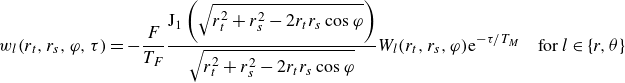 \begin{align} w_l(r_t, r_s, \varphi , \tau ) = -\frac {F}{T_F} \frac {\textrm{J}_1\left (\sqrt {r_t^2 + r_s^2 - 2r_tr_s\cos \varphi }\right )}{\sqrt {r_t^2 + r_s^2 - 2r_tr_s\cos \varphi }}W_l(r_t,r_s,\varphi )\textrm{e}^{-\tau /T_M} \quad \mbox{for } l \in \{r, \theta \} \end{align}
are the radial and tangential components of the memory kernel, defined in terms of the current, $r_t = r(t)$
, and prior,
$r_t = r(t)$
, and prior, $r_s = r(s)$
, radial position, the change in polar angle,
$r_s = r(s)$
, radial position, the change in polar angle, $\varphi = \theta (t) - \theta (s)$
, and the change in time,
$\varphi = \theta (t) - \theta (s)$
, and the change in time, $\tau = t-s$
, where
$\tau = t-s$
, where $W_r = r_t - r_s\cos \varphi$
and
$W_r = r_t - r_s\cos \varphi$
and $W_\theta = r_s\sin \varphi$
. Finally, the magnitude of the perturbation is governed by the small parameter
$W_\theta = r_s\sin \varphi$
. Finally, the magnitude of the perturbation is governed by the small parameter $0 \lt \epsilon \ll 1$
, with
$0 \lt \epsilon \ll 1$
, with $C_r = c_r$
and
$C_r = c_r$
and $C_\theta = r_0 c_\theta$
appearing in (B2) being arbitrary constants.
$C_\theta = r_0 c_\theta$
appearing in (B2) being arbitrary constants.
The droplet also evolves in response to the radial and tangential components on the external force field. For a Coriolis force, $\boldsymbol{F} = -2m\boldsymbol{\Omega }\times \,\dot {\!\boldsymbol{x}\!}_p$
, the external force parameter,
$\boldsymbol{F} = -2m\boldsymbol{\Omega }\times \,\dot {\!\boldsymbol{x}\!}_p$
, the external force parameter, $\zeta$
, in (B2) is equal to the rotation rate,
$\zeta$
, in (B2) is equal to the rotation rate, $\Omega$
, and the radial and tangential force components are
$\Omega$
, and the radial and tangential force components are
 \begin{equation} f_{{ext},r}(r,\dot {r},\dot {\theta }) = -2mr\dot \theta \quad \mbox{and}\quad f_{{ext},\theta }(r,\dot {r},\dot {\theta }) = 2m \dot r. \end{equation}
For an attractive central force of the form $\boldsymbol{F} = -kF(|\boldsymbol{x\!}_p|)\boldsymbol{x\!}_p$
with
$\boldsymbol{F} = -kF(|\boldsymbol{x\!}_p|)\boldsymbol{x\!}_p$
with $F(r) \gt 0$
, we set
$F(r) \gt 0$
, we set $\zeta$
equal to the spring constant,
$\zeta$
equal to the spring constant, $k$
. The radial and tangential force components are thus
$k$
. The radial and tangential force components are thus
 \begin{equation} f_{{ext},r}(r,\dot {r},\dot {\theta }) = F(r)r \quad \mbox{and}\quad f_{{ext},\theta }(r,\dot {r},\dot {\theta }) = 0. \end{equation}
Notably, the tangential component of the external force, $f_{{ext},\theta }$
, vanishes for steady orbital motion in the presence of either a Coriolis force or a central force, which we leverage in our analysis below. Recasting the radial and tangential force balances in the form (B2) allows us to streamline algebra and highlight the key features of the stability framework. Our analysis encompasses the results of Oza et al. (Reference Oza, Harris, Rosales and Bush2014a
) and Labousse et al. (Reference Labousse, Oza, Perrard and Bush2016) for a droplet orbiting in response to a Coriolis or central force, respectively.
$f_{{ext},\theta }$
, vanishes for steady orbital motion in the presence of either a Coriolis force or a central force, which we leverage in our analysis below. Recasting the radial and tangential force balances in the form (B2) allows us to streamline algebra and highlight the key features of the stability framework. Our analysis encompasses the results of Oza et al. (Reference Oza, Harris, Rosales and Bush2014a
) and Labousse et al. (Reference Labousse, Oza, Perrard and Bush2016) for a droplet orbiting in response to a Coriolis or central force, respectively.
B.1. Linear stability analysis
To analyse the linear stability of circular orbits, we assume that the droplet executes a circular orbit of radius $r_0$
and angular frequency
$r_0$
and angular frequency $\omega$
for all
$\omega$
for all $t \lt 0$
. Following Oza (Reference Oza2014) and Liu et al. (Reference Liu, Durey and Bush2023), we parametrise steady circular orbits in terms of their orbital radius. We express the corresponding angular frequency as
$t \lt 0$
. Following Oza (Reference Oza2014) and Liu et al. (Reference Liu, Durey and Bush2023), we parametrise steady circular orbits in terms of their orbital radius. We express the corresponding angular frequency as $\omega = \omega _0(r_0)$
, and the force coefficient required to sustain the circular orbit as
$\omega = \omega _0(r_0)$
, and the force coefficient required to sustain the circular orbit as $\zeta = \zeta _0(r_0)$
. It follows that
$\zeta = \zeta _0(r_0)$
. It follows that $\omega _0(r_0)$
and
$\omega _0(r_0)$
and $\zeta _0(r_0)$
satisfy the force balance equations
$\zeta _0(r_0)$
satisfy the force balance equations $F_r(r_0,\omega _0(r_0),\zeta _0(r_0)) = 0$
and
$F_r(r_0,\omega _0(r_0),\zeta _0(r_0)) = 0$
and $F_\theta (r_0,\omega _0(r_0)) = 0$
(see 3.3), where
$F_\theta (r_0,\omega _0(r_0)) = 0$
(see 3.3), where
 \begin{align}& F_r(r_0,\omega ,\zeta ) = f_r(r_0,0,0,\omega ,0) + \zeta f_{{ext},r}(r_0,0,\omega ) + \int _0^\infty w_r(r_0,r_0,\omega t,t)\,\textrm{d}t, \end{align}
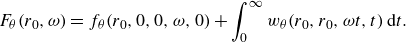 \begin{align}&\qquad\qquad\quad F_\theta (r_0,\omega ) = f_\theta (r_0,0,0,\omega ,0) + \int _0^\infty w_\theta (r_0,r_0,\omega t,t)\,\textrm{d}t. \end{align}
We note that the independence of $F_\theta$
on the force parameter,
$F_\theta$
on the force parameter, $\zeta$
, is a direct consequence of a vanishing tangential force,
$\zeta$
, is a direct consequence of a vanishing tangential force, $f_{{ext},\theta }(r_0, 0, \omega ) = 0$
, for steady orbital motion in the presence of a Coriolis or central force. In addition, the first two arguments of
$f_{{ext},\theta }(r_0, 0, \omega ) = 0$
, for steady orbital motion in the presence of a Coriolis or central force. In addition, the first two arguments of $w_r$
and
$w_r$
and $w_\theta$
are both evaluated at
$w_\theta$
are both evaluated at $r_0$
to reflect the fact that the past trajectory is the circular orbit.
$r_0$
to reflect the fact that the past trajectory is the circular orbit.
To account for the influence of the infinitesimal forcing at $t = 0$
on the droplet motion for
$t = 0$
on the droplet motion for $t \gt 0$
, we substitute the ansatz
$t \gt 0$
, we substitute the ansatz $r(t) = r_0 + \epsilon H(t) r_1(t)$
and
$r(t) = r_0 + \epsilon H(t) r_1(t)$
and $\theta (t) = \omega t + \epsilon H(t) \theta _1(t)$
into (B2), where
$\theta (t) = \omega t + \epsilon H(t) \theta _1(t)$
into (B2), where $r_1$
and
$r_1$
and $\theta _1$
are the perturbed radius and polar angle, and
$\theta _1$
are the perturbed radius and polar angle, and $H(t)$
denotes the Heaviside function. As the droplet position is continuous for all time, we conclude that
$H(t)$
denotes the Heaviside function. As the droplet position is continuous for all time, we conclude that $r_1(0) = \theta _1(0) = 0$
; however, the acceleration impulse gives rise to a jump in droplet velocity, yielding
$r_1(0) = \theta _1(0) = 0$
; however, the acceleration impulse gives rise to a jump in droplet velocity, yielding $({\partial {f_r}}/{\partial {\ddot {r}}})\dot {r}_1(0^+) = c_r$
and
$({\partial {f_r}}/{\partial {\ddot {r}}})\dot {r}_1(0^+) = c_r$
and $({\partial {f_\theta }}/{\partial {\ddot {\theta }}})\dot {\theta }_1(0^+) = r_0 c_\theta$
(Oza et al. Reference Oza, Harris, Rosales and Bush2014a
; Liu et al. Reference Liu, Durey and Bush2023), where
$({\partial {f_\theta }}/{\partial {\ddot {\theta }}})\dot {\theta }_1(0^+) = r_0 c_\theta$
(Oza et al. Reference Oza, Harris, Rosales and Bush2014a
; Liu et al. Reference Liu, Durey and Bush2023), where
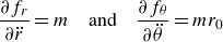 \begin{equation} \frac {\partial {f_r}}{\partial {\ddot {r}}} = m \quad \mbox{and}\quad \frac {\partial {f_\theta }}{\partial {\ddot {\theta }}} = mr_0 \end{equation}
for steady orbital motion with radius $r_0$
.
$r_0$
.
By denoting the Laplace transforms of $r_1(t)$
and
$r_1(t)$
and $\theta _1(t)$
as
$\theta _1(t)$
as $R(s) = \mathscr{L}[r_1](s)$
and
$R(s) = \mathscr{L}[r_1](s)$
and $\Theta (s) = \mathscr{L}[\theta _1](s)$
, respectively, the Laplace transforms of the linearised evolution equations yield
$\Theta (s) = \mathscr{L}[\theta _1](s)$
, respectively, the Laplace transforms of the linearised evolution equations yield
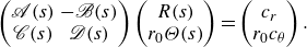 \begin{gather} \begin{pmatrix}\mathscr{A}(s) & -\mathscr{B}(s) \\ \mathscr{C}(s) & \mathscr{D}(s) \end{pmatrix}\begin{pmatrix} R(s) \\ r_0\Theta (s)\end{pmatrix} = \begin{pmatrix} c_r \\ r_0 c_\theta \end{pmatrix}. \end{gather}
The functions in (B9) are defined in terms of $\textrm{f}_r = f_r + \zeta f_{{ext},r}$
and
$\textrm{f}_r = f_r + \zeta f_{{ext},r}$
and $\textrm{f}_\theta = f_\theta + \zeta f_{{ext},\theta }$
by
$\textrm{f}_\theta = f_\theta + \zeta f_{{ext},\theta }$
by
 \begin{align}& \mathscr{A}(s) = \left [\frac {\partial {\textrm{f}_r}}{\partial {r}} + s\frac {\partial {\textrm{f}_r}}{\partial {\dot {r}}} + s^2\frac {\partial {\textrm{f}_r}}{\partial {\ddot {r}}}\right ]_O + \int _0^\infty \!\frac {\partial {w_r}}{\partial {r_t}}(r_0,r_0,\omega t,t)\,\textrm{d}t + \mathscr{L}\left [\frac {\partial {w_r}}{\partial {r_s}}(r_0,r_0,\omega t,t)\right ]\!, \end{align}
 \begin{align}& -r_0\mathscr{B}(s) = \left [s\frac {\partial {\textrm{f}_r}}{\partial {\dot {\theta }}} + s^2\frac {\partial {\textrm{f}_r}}{\partial {\ddot {\theta }}}\right ]_O + \int _0^\infty \!\frac {\partial {w_r}}{\partial {\varphi }}(r_0,r_0,\omega t,t)\,\textrm{d}t - \mathscr{L}\left [\frac {\partial {w_r}}{\partial {\varphi }}(r_0,r_0,\omega t,t)\right ], \end{align}
where $\mathscr{C}$
and
$\mathscr{C}$
and $\mathscr{D}$
are defined the same as
$\mathscr{D}$
are defined the same as $\mathscr{A}$
and
$\mathscr{A}$
and $-\mathscr{B}$
, respectively, but with
$-\mathscr{B}$
, respectively, but with $\textrm{f}_r$
replaced by
$\textrm{f}_r$
replaced by $\textrm{f}_\theta$
and
$\textrm{f}_\theta$
and $w_r$
replaced by
$w_r$
replaced by $w_\theta$
. In (B10), the notation
$w_\theta$
. In (B10), the notation $[F]_O$
means that the function
$[F]_O$
means that the function $F$
is evaluated for a steady circular orbit, so
$F$
is evaluated for a steady circular orbit, so $[f_r]_O = f_r(r_0, 0, 0, \omega , 0)$
, for example. The stability coefficients in (B11) are equivalent to those detailed in (C1). Finally, the asymptotic growth rates,
$[f_r]_O = f_r(r_0, 0, 0, \omega , 0)$
, for example. The stability coefficients in (B11) are equivalent to those detailed in (C1). Finally, the asymptotic growth rates, $s$
, governing the perturbation evolution are the poles of (B9) and thus satisfy
$s$
, governing the perturbation evolution are the poles of (B9) and thus satisfy $\mathscr{F}(s) = 0$
, where
$\mathscr{F}(s) = 0$
, where
 \begin{equation} \mathscr{F}(s) = \mathscr{A}(s) \mathscr{D}(s) + \mathscr{B}(s) \mathscr{C}(s). \end{equation}
B.2. Properties of the stability function
We proceed to establish the behaviour of $\mathscr{F}(s)$
for small
$\mathscr{F}(s)$
for small $s$
, which we will use to prove Theorem1. In particular, rotational invariance of the pilot-wave system renders
$s$
, which we will use to prove Theorem1. In particular, rotational invariance of the pilot-wave system renders $\mathscr{B}(0) = \mathscr{D}(0) = 0$
and, hence,
$\mathscr{B}(0) = \mathscr{D}(0) = 0$
and, hence, $\mathscr{F}(0) = 0$
. We thus conclude that
$\mathscr{F}(0) = 0$
. We thus conclude that
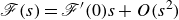 \begin{equation} \mathscr{F}(s) = \mathscr{F}'(0) s + O(s^2) \end{equation}
for sufficiently small $s$
, where
$s$
, where $ \mathscr{F}'(0) = \mathscr{A}(0)\mathscr{D}'(0) + \mathscr{B}'(0)\mathscr{C}(0).$
In fact, the stability coefficients in this case are very closely related to the equilibrium force balances (B7), with
$ \mathscr{F}'(0) = \mathscr{A}(0)\mathscr{D}'(0) + \mathscr{B}'(0)\mathscr{C}(0).$
In fact, the stability coefficients in this case are very closely related to the equilibrium force balances (B7), with
 \begin{align} \mathscr{A}(0) &= \left [\frac {\partial {\textrm{f}_r}}{\partial {r}}\right ]_O + \int _0^\infty \left [\frac {\partial {w_r}}{\partial {r_t}}(r_0,r_0,\omega t,t) + \frac {\partial {w_r}}{\partial {r_s}}(r_0,r_0,\omega t,t)\right ]\,\textrm{d}t = \frac {\partial {F_r}}{\partial {r_0}}, \end{align}
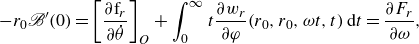 \begin{align} -r_0\mathscr{B}'(0) &= \left [\frac {\partial {\textrm{f}_r}}{\partial {\dot {\theta }}}\right ]_O + \int _0^\infty t\frac {\partial {w_r}}{\partial {\varphi }}(r_0,r_0,\omega t,t)\,\textrm{d}t = \frac {\partial {F_r}}{\partial {\omega }}, \end{align}
and likewise
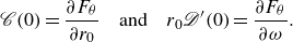 \begin{equation} \mathscr{C}(0) = \frac {\partial {F_\theta }}{\partial {r_0}} \quad \mbox{and} \quad r_0\mathscr{D}'(0) = \frac {\partial {F_\theta }}{\partial {\omega }}. \end{equation}
We may thus equivalently write
 \begin{equation} r_0\mathscr{F}'(0) = \frac {\partial {F_r}}{\partial {r_0}}\frac {\partial {F_\theta }}{\partial {\omega }} - \frac {\partial {F_r}}{\partial {\omega }}\frac {\partial {F_\theta }}{\partial {r_0}}, \end{equation}
where all derivatives are understood to be evaluated for $(r_0, \omega , \zeta )$
.
$(r_0, \omega , \zeta )$
.
The relationship (B13) can be simplified further so as to deduce a more explicit expression for $\mathscr{F}'(0)$
. To do so, we differentiate the force balance equations
$\mathscr{F}'(0)$
. To do so, we differentiate the force balance equations $F_r(r_0, \omega _0(r_0), \zeta _0(r_0)) = 0$
and
$F_r(r_0, \omega _0(r_0), \zeta _0(r_0)) = 0$
and $F_\theta (r_0, \omega _0(r_0)) = 0$
(see B7) with respect to
$F_\theta (r_0, \omega _0(r_0)) = 0$
(see B7) with respect to $r_0$
, giving (Oza et al. Reference Oza, Harris, Rosales and Bush2014a
)
$r_0$
, giving (Oza et al. Reference Oza, Harris, Rosales and Bush2014a
)
 \begin{gather} \frac {\partial {F_r}}{\partial {r_0}} + \frac {\partial {F_r}}{\partial {\omega }}\frac {\textrm{d} {\omega _0}}{\textrm{d}{r_0}} + f_{{ext},r}\frac {\textrm{d} {\zeta _0}}{\textrm{d}{r_0}} = 0,\quad \frac {\partial {F_\theta }}{\partial {r_0}} + \frac {\partial {F_\theta }}{\partial {\omega }}\frac {\textrm{d} {\omega _0}}{\textrm{d}{r_0}} = 0. \end{gather}
By eliminating $\textrm{d}\omega _0/\textrm{d}r_0$
from (B15), we find that
$\textrm{d}\omega _0/\textrm{d}r_0$
from (B15), we find that
 \begin{align} \left \{\frac {\partial {F_r}}{\partial {r_0}}\frac {\partial {F_\theta }}{\partial {\omega }} - \frac {\partial {F_r}}{\partial {\omega }}\frac {\partial {F_\theta }}{\partial {r_0}}\right \} + f_{{ext},r}\frac {\textrm{d} {\zeta _0}}{\textrm{d}{r_0}}\frac {\partial {F_\theta }}{\partial {\omega }} = 0, \end{align}
where upon applying (B14) to the term in curly brackets immediately yields the relationship
 \begin{align} r_0\mathscr{F}'(0) + f_{{ext},r}\frac {\textrm{d} {\zeta _0}}{\textrm{d}{r_0}} \frac {\partial {F_\theta }}{\partial {\omega }} = 0. \end{align}
Finally, we simplify the triple product by noting that the third term may be replaced by $r_0\mathscr{D}'(0)$
using (B13c
), giving
$r_0\mathscr{D}'(0)$
using (B13c
), giving
 \begin{gather} \mathscr{F}'(0) = - f_{{ext},r}(r_0, 0, \omega )\frac {\textrm{d} {\zeta _0}}{\textrm{d}{r_0}}\mathscr{D}'(0). \end{gather}
This algebraic form generalises a similar result obtained by Oza et al. (Reference Oza, Harris, Rosales and Bush2014a ), and will be leveraged in the proof of Theorem1.
Theorem 1.
Consider orbital solutions satisfying $F_r(r_0, \omega _0(r_0), \zeta _0(r_0)) = 0$
and
$F_r(r_0, \omega _0(r_0), \zeta _0(r_0)) = 0$
and $F_\theta (r_0, \omega _0(r_0)) = 0$
(as defined in B7), where the angular frequency,
$F_\theta (r_0, \omega _0(r_0)) = 0$
(as defined in B7), where the angular frequency, $\omega = \omega _0(r_0)$
, and force coefficient,
$\omega = \omega _0(r_0)$
, and force coefficient, $\zeta = \zeta _0(r_0)$
, are parametrised by the orbital radius,
$\zeta = \zeta _0(r_0)$
, are parametrised by the orbital radius, $r_0$
. The orbital solution is unstable with a real and positive root of
$r_0$
. The orbital solution is unstable with a real and positive root of $\mathscr{F}(s)$
(as defined in B11) in each of the following cases: (i)
$\mathscr{F}(s)$
(as defined in B11) in each of the following cases: (i) $\omega \, \textrm{d}\Omega _0/\textrm{d}r_0 \lt 0$
for a Coriolis force,
$\omega \, \textrm{d}\Omega _0/\textrm{d}r_0 \lt 0$
for a Coriolis force, $\boldsymbol{F} = -2m\boldsymbol{\Omega }\times \,\dot {\!\boldsymbol{x}\!}_p$
, where the force coefficient is the bath rotation rate,
$\boldsymbol{F} = -2m\boldsymbol{\Omega }\times \,\dot {\!\boldsymbol{x}\!}_p$
, where the force coefficient is the bath rotation rate, $\zeta = \Omega$
; (ii)
$\zeta = \Omega$
; (ii) $\textrm{d}k_0/\textrm{d}r_0 \gt 0$
for an attractive central force,
$\textrm{d}k_0/\textrm{d}r_0 \gt 0$
for an attractive central force, $\boldsymbol{F} = -kF(|\boldsymbol{x\!}_p|)\boldsymbol{x\!}_p$
with
$\boldsymbol{F} = -kF(|\boldsymbol{x\!}_p|)\boldsymbol{x\!}_p$
with $F(r) \gt 0$
, where the force coefficient is the spring stiffness,
$F(r) \gt 0$
, where the force coefficient is the spring stiffness, $\zeta = k$
.
$\zeta = k$
.
Proof.
The proof uses the intermediate value theorem to establish a sufficient condition for there to exist a real and positive root of the stability function $\mathscr{F}(s)$
, which we then apply for the cases of Coriolis or central forces. As all Laplace transforms in (B10) decay to zero as
$\mathscr{F}(s)$
, which we then apply for the cases of Coriolis or central forces. As all Laplace transforms in (B10) decay to zero as $s\rightarrow \infty$
, we first note that
$s\rightarrow \infty$
, we first note that
 \begin{align} \mathscr{F}(s) \sim c_\infty s^4 \quad \mbox{as } s\rightarrow \infty , \quad \mbox{where } c_\infty = \frac {1}{r_0}\left [\frac {\partial {f_r}}{\partial {\ddot {r}}}\frac {\partial {f_\theta }}{\partial {\ddot {\theta }}} - \frac {\partial {f_r}}{\partial {\ddot {\theta }}}\frac {\partial {f_\theta }}{\partial {\ddot {r}}}\right ]_O = m^2 \gt 0, \end{align}
as may be evaluated using (B8) and ${\partial {f_r}}/{\partial {\ddot {\theta }}} = {\partial {f_\theta }}/{\partial {\ddot {r}}} = 0$
(see B3). There thus exists a real and positive root of
${\partial {f_r}}/{\partial {\ddot {\theta }}} = {\partial {f_\theta }}/{\partial {\ddot {r}}} = 0$
(see B3). There thus exists a real and positive root of $\mathscr{F}(s)$
if
$\mathscr{F}(s)$
if $\mathscr{F}'(0) \lt 0$
(see B12). From (B18), this condition is equivalent to
$\mathscr{F}'(0) \lt 0$
(see B12). From (B18), this condition is equivalent to
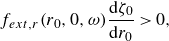 \begin{equation} f_{{ext},r}(r_0, 0, \omega )\frac {\textrm{d} {\zeta _0}}{\textrm{d}{r_0}} \gt 0, \end{equation}
where we have used that $\mathscr{D}'(0) \gt 0$
for the stroboscopic model (see the proof in Appendix F). We proceed by evaluating
$\mathscr{D}'(0) \gt 0$
for the stroboscopic model (see the proof in Appendix F). We proceed by evaluating $f_{{ext},r}(r_0, 0, \omega )$
for Coriolis and central forces to establish sufficient conditions on the sign of
$f_{{ext},r}(r_0, 0, \omega )$
for Coriolis and central forces to establish sufficient conditions on the sign of $\textrm{d}\zeta _0/\textrm{d}r_0$
, as follows.
$\textrm{d}\zeta _0/\textrm{d}r_0$
, as follows.
For a Coriolis force, we recall that $\zeta _0 = \Omega _0$
and that
$\zeta _0 = \Omega _0$
and that $f_{{ext},r}(r_0, 0, \omega ) = -2m r_0 \omega$
(see B5), the sign of which depends on
$f_{{ext},r}(r_0, 0, \omega ) = -2m r_0 \omega$
(see B5), the sign of which depends on $\omega$
. We thus deduce from (B20) that there exists a real and positive root of
$\omega$
. We thus deduce from (B20) that there exists a real and positive root of $\mathscr{F}(s)$
when
$\mathscr{F}(s)$
when $\omega \, \textrm{d}\Omega _0/\textrm{d}r_0 \lt 0$
, which proves case (i).
$\omega \, \textrm{d}\Omega _0/\textrm{d}r_0 \lt 0$
, which proves case (i).
For a central force, we recall that $\zeta _0 = k_0$
and that
$\zeta _0 = k_0$
and that $f_{{ext},r}(r_0, 0, \omega ) = r_0 F(r_0) \gt 0$
(see B6). We thus deduce from (B20) that there exists a real and positive root of
$f_{{ext},r}(r_0, 0, \omega ) = r_0 F(r_0) \gt 0$
(see B6). We thus deduce from (B20) that there exists a real and positive root of $\mathscr{F}(s)$
when
$\mathscr{F}(s)$
when $\textrm{d}k_0/\textrm{d}r_0 \gt 0$
, which proves case (ii).
$\textrm{d}k_0/\textrm{d}r_0 \gt 0$
, which proves case (ii).
Theorem1 determines the onset of monotonically growing orbital instabilities without needing to consider the fully stability problem (B11). For a Coriolis force, the theorem statement is identical to Theorem 1 of Oza et al. (Reference Oza, Harris, Rosales and Bush2014a
), except we prove explicitly the bound $\mathscr{D}'(0) \gt 0$
in Appendix F, a result that had previously been only verified numerically (Oza Reference Oza2014). Furthermore, Theorem1 extends the work of Oza et al. (Reference Oza, Harris, Rosales and Bush2014a
) to orbiting in attractive central forces, sidestepping the details of the pilot-wave system. This relative generality suggests that Theorem1 is a fundamental property of orbital stability across a wide class of Coriolis and central force systems. Our proof also applies to non-Bessel wave kernels (with the proviso that
$\mathscr{D}'(0) \gt 0$
in Appendix F, a result that had previously been only verified numerically (Oza Reference Oza2014). Furthermore, Theorem1 extends the work of Oza et al. (Reference Oza, Harris, Rosales and Bush2014a
) to orbiting in attractive central forces, sidestepping the details of the pilot-wave system. This relative generality suggests that Theorem1 is a fundamental property of orbital stability across a wide class of Coriolis and central force systems. Our proof also applies to non-Bessel wave kernels (with the proviso that $\mathscr{D}'(0) \gt 0$
), as are needed to model the exponential far-field decay of the bouncer wave field (Damiano et al. Reference Damiano, Brun, Harris, Galeano-Rios and Bush2016; Tadrist et al. Reference Tadrist, Shim, Gilet and Schlagheck2018; Turton et al. Reference Turton, Couchman and Bush2018).
$\mathscr{D}'(0) \gt 0$
), as are needed to model the exponential far-field decay of the bouncer wave field (Damiano et al. Reference Damiano, Brun, Harris, Galeano-Rios and Bush2016; Tadrist et al. Reference Tadrist, Shim, Gilet and Schlagheck2018; Turton et al. Reference Turton, Couchman and Bush2018).
The physical interpretation of Theorem1 for a central force is as follows, with the interpretation for inertial orbits in a Coriolis force being similar. Specifically, we rationalise the onset of monotonic instabilities through consideration of a perturbation from a circular orbit of radius $r_0$
with fixed spring constant
$r_0$
with fixed spring constant $k_* = k_0(r_0)$
. The perturbation is assumed to grow slowly, with the perturbed trajectory remaining nearly circular for all time; thus, the force balance equations (3.3) may be used to characterise the perturbed orbit. In the following argument, we denote the droplet’s instantaneous radial position by
$k_* = k_0(r_0)$
. The perturbation is assumed to grow slowly, with the perturbed trajectory remaining nearly circular for all time; thus, the force balance equations (3.3) may be used to characterise the perturbed orbit. In the following argument, we denote the droplet’s instantaneous radial position by $r(t)$
and assume that
$r(t)$
and assume that $\textrm{d}k_0/\textrm{d}r_0 \gt 0$
. For outward perturbations, the spring constant
$\textrm{d}k_0/\textrm{d}r_0 \gt 0$
. For outward perturbations, the spring constant $k_*$
will be less than that needed for steady orbital motion at radius
$k_*$
will be less than that needed for steady orbital motion at radius $r(t)$
, as
$r(t)$
, as $k_* \lt k_0(r)$
when
$k_* \lt k_0(r)$
when $r(t) \gt r_0$
. Likewise, the spring constant,
$r(t) \gt r_0$
. Likewise, the spring constant, $k_*$
, will exceed that needed for steady orbital motion at radius
$k_*$
, will exceed that needed for steady orbital motion at radius $r(t)$
for inward perturbations, since
$r(t)$
for inward perturbations, since $k_* \gt k_0(r)$
when
$k_* \gt k_0(r)$
when $r(t) \lt r_0$
. Consequently, outward perturbations lead to a net outward radial force and inward perturbations result in a net inward force, causing the droplet’s radial position to increase or decrease monotonically in time upon perturbation.
$r(t) \lt r_0$
. Consequently, outward perturbations lead to a net outward radial force and inward perturbations result in a net inward force, causing the droplet’s radial position to increase or decrease monotonically in time upon perturbation.
Appendix C. Orbital stability for pilot-wave hydrodynamics
As outlined in Appendix B, the asymptotic growth rates, $s$
, associated with a perturbation from a circular orbit of radius
$s$
, associated with a perturbation from a circular orbit of radius $r_0$
and angular frequency
$r_0$
and angular frequency $\omega$
are precisely the roots of the stability function
$\omega$
are precisely the roots of the stability function $\mathscr{F}(s) = \mathscr{A}(s)\mathscr{D}(s) + \mathscr{B}(s)\mathscr{C}(s)$
, which is defined in terms of the coefficients
$\mathscr{F}(s) = \mathscr{A}(s)\mathscr{D}(s) + \mathscr{B}(s)\mathscr{C}(s)$
, which is defined in terms of the coefficients
 \begin{align} \mathscr{A}(s) &= m(s^2 + (n-1)\omega ^2) + D\left (s + \frac {1}{T_M}\right )\nonumber\\&\quad + F k_F\left [ \mathcal{C}_0(s) + \mathcal{I}_1(s) -\frac {n+1}{k_F^2 r_0}\frac {\partial {\mathcal{I}_0(0)}}{\partial {r_0}} - 2\mathcal{I}_0(0)\right ], \end{align}
 \begin{align} \mathscr{B}(s) &= (2-\varDelta )m\omega s + F k_F\left [ \left (s\Delta - \frac {1}{T_M}\right )\frac {1}{k_F^2 r_0\omega }\frac {\partial {\mathcal{I}_0(0)}}{\partial {r_0}} - \mathcal{S}_0(s)\right ], \end{align}
 \begin{align} \mathscr{C}(s) &= (2-\varDelta )m\omega s + 2D\omega + F k_F\left [ \left (s\Delta + \frac {1}{T_M}\right )\frac {1}{k_F^2 r_0\omega }\frac {\partial {\mathcal{I}_0(0)}}{\partial {r_0}} - \mathcal{S}_0(s)\right ], \end{align}
 \begin{align} \mathscr{D}(s) &= m s^2 + D\left (s - \frac {1}{T_M}\right ) + F k_F\left [\mathcal{C}_0(s) - \mathcal{I}_1(s)\right ]. \end{align}
The indicator $\varDelta \in \{0, 1\}$
determines the type of applied force, with
$\varDelta \in \{0, 1\}$
determines the type of applied force, with $\varDelta = 0$
for a power-law central force of the form
$\varDelta = 0$
for a power-law central force of the form $\boldsymbol{F} = -k|\boldsymbol{x\!}_p|^{n-1}\boldsymbol{x\!}_p$
and
$\boldsymbol{F} = -k|\boldsymbol{x\!}_p|^{n-1}\boldsymbol{x\!}_p$
and $\varDelta = 1$
for a Coriolis force,
$\varDelta = 1$
for a Coriolis force, $\boldsymbol{F} = -2m \boldsymbol{\Omega }\times \,\dot {\!\boldsymbol{x}\!}_p$
. For a Coriolis force, we additionally set
$\boldsymbol{F} = -2m \boldsymbol{\Omega }\times \,\dot {\!\boldsymbol{x}\!}_p$
. For a Coriolis force, we additionally set $n = 1$
in (C1). The stability coefficients are defined in terms of the following integrals (for all integers
$n = 1$
in (C1). The stability coefficients are defined in terms of the following integrals (for all integers $m \geqslant 0$
and
$m \geqslant 0$
and $T_M\textrm{Re}(s) \gt -1$
):
$T_M\textrm{Re}(s) \gt -1$
):
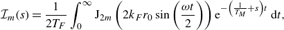 \begin{align} \mathcal{I}_m(s) &= \frac {1}{2T_F}\int _0^\infty \textrm{J}_{2m}\left (2k_F r_0\sin \left (\frac {\omega t}{2}\right )\right )\textrm{e}^{-\left (\frac {1}{T_M}+s\right )t}\,\textrm{d}t, \end{align}
 \begin{align} \mathcal{C}_m(s) &= \frac {1}{2T_F}\int _0^\infty \textrm{J}_{2m}\left (2k_F r_0\sin \left (\frac {\omega t}{2}\right )\right )\cos (\omega t)\textrm{e}^{-\left (\frac {1}{T_M}+s\right )t}\,\textrm{d}t \end{align}
 \begin{align} \textrm{and}\quad \mathcal{S}_m(s) &= \frac {1}{2T_F}\int _0^\infty \textrm{J}_{2m}\left (2k_F r_0\sin \left (\frac {\omega t}{2}\right )\right )\sin (\omega t)\textrm{e}^{-\left (\frac {1}{T_M}+s\right )t}\,\textrm{d}t. \end{align}
These integrals encode the effects of path memory on the response of the walking droplet to perturbations from a circular orbit. Finally, we use integration by parts to recast the tangential force balance (3.3b
) (with $\boldsymbol{F}\cdot \boldsymbol{t} = 0$
) in terms of the stability integral
$\boldsymbol{F}\cdot \boldsymbol{t} = 0$
) in terms of the stability integral $\mathcal{I}_0$
, giving
$\mathcal{I}_0$
, giving
 \begin{gather} \frac {2T_F}{T_M}\mathcal{I}_0(0) = 1 - \frac {r_0^2\omega ^2}{c^2}, \end{gather}
where $c = \sqrt {F/DT_F k_F}$
is the maximum steady orbital speed (Liu et al. Reference Liu, Durey and Bush2023).
$c = \sqrt {F/DT_F k_F}$
is the maximum steady orbital speed (Liu et al. Reference Liu, Durey and Bush2023).
In summary, the orbital stability problem requires solving $\mathscr{F}(s) = 0$
and (C3) for
$\mathscr{F}(s) = 0$
and (C3) for $s$
and
$s$
and $\omega$
, respectively, for a given orbital radius,
$\omega$
, respectively, for a given orbital radius, $r_0$
(Oza Reference Oza2014; Oza et al. Reference Oza, Harris, Rosales and Bush2014a
), and is defined in terms of the stability coefficients (C1) and integrals (C2). The stability coefficients depend explicitly on the form of the applied force, as indicated by
$r_0$
(Oza Reference Oza2014; Oza et al. Reference Oza, Harris, Rosales and Bush2014a
), and is defined in terms of the stability coefficients (C1) and integrals (C2). The stability coefficients depend explicitly on the form of the applied force, as indicated by $\varDelta \in \{0,1\}$
in (C1). The stability integrals (C2) may be evaluated analytically (Liu et al. Reference Liu, Durey and Bush2023, Appendix B), either in terms of Bessel functions of complex order,
$\varDelta \in \{0,1\}$
in (C1). The stability integrals (C2) may be evaluated analytically (Liu et al. Reference Liu, Durey and Bush2023, Appendix B), either in terms of Bessel functions of complex order,
 \begin{gather} \mathcal{I}_m(s) = \frac {\pi }{2\omega T_F}\textrm{J}_{m+\textrm{i}\eta }(k_F r_0)\textrm{J}_{m-\textrm{i}\eta }(k_F r_0){\textrm {csch}}(\pi \eta ), \end{gather}
or in terms of infinite sums,
 \begin{gather} \mathcal{I}_m(s) = \frac {\eta }{2\omega T_F}\sum _{n=-\infty }^\infty \frac {(-1)^n\textrm{J}_{m+n}(k_F r_0)\textrm{J}_{m-n}(k_F r_0)}{\eta ^2 + n^2}, \end{gather}
with
 \begin{equation} \mathcal{C}_m(s) = \frac {1}{2}\left (\mathcal{I}_m(s+\textrm{i}\omega ) + \mathcal{I}_m(s-\textrm{i}\omega )\right ), \quad \mathcal{S}_m(s) = \frac {1}{2\textrm{i}}\left (\mathcal{I}_m(s-\textrm{i} \omega ) - \mathcal{I}_m(s+\textrm{i}\omega )\right ) \end{equation}
and $\eta = (s + T_M^{-1} )/\omega$
. Finally, we note that the various combinations of stability integrals appearing in (C1) may be reduced to a more concise form (Liu et al. Reference Liu, Durey and Bush2023, Appendix B).
$\eta = (s + T_M^{-1} )/\omega$
. Finally, we note that the various combinations of stability integrals appearing in (C1) may be reduced to a more concise form (Liu et al. Reference Liu, Durey and Bush2023, Appendix B).
The orbital solution is unstable if there are any roots, $s$
, of
$s$
, of $\mathscr{F}$
satisfying
$\mathscr{F}$
satisfying $\text{Re}(s) \gt 0$
. By denoting
$\text{Re}(s) \gt 0$
. By denoting $s_*$
as the unstable root with largest real part, the instability is monotonic if
$s_*$
as the unstable root with largest real part, the instability is monotonic if $\text{Im}(s_*) = 0$
and oscillatory otherwise. The stability function,
$\text{Im}(s_*) = 0$
and oscillatory otherwise. The stability function, $\mathscr{F}$
, has a trivial eigenvalue at
$\mathscr{F}$
, has a trivial eigenvalue at $0$
, corresponding to rotational invariance of the orbital motion. In the case of the Coriolis force,
$0$
, corresponding to rotational invariance of the orbital motion. In the case of the Coriolis force, $\mathscr{F}$
has additional trivial eigenvalues at
$\mathscr{F}$
has additional trivial eigenvalues at $\pm \textrm{i}\omega$
due to translational invariance (Oza et al. Reference Oza, Harris, Rosales and Bush2014a
). It follows that the non-trivial roots of the stability problem satisfy
$\pm \textrm{i}\omega$
due to translational invariance (Oza et al. Reference Oza, Harris, Rosales and Bush2014a
). It follows that the non-trivial roots of the stability problem satisfy $\mathscr{G}(s) = 0$
, where
$\mathscr{G}(s) = 0$
, where
 \begin{align} \mathscr{G}_{{Cor.}}(s) = \frac {\mathscr{A}(s)\mathscr{D}(s) + \mathscr{B}(s)\mathscr{C}(s)}{s(s^2+\omega ^2)} \quad \mbox{and}\quad \mathscr{G}_{{spr.}}(s) = \frac {\mathscr{A}(s)\mathscr{D}(s) + \mathscr{B}(s)\mathscr{C}(s)}{s}. \end{align}
We apply the method of Delves & Lyness (Reference Delves and Lyness1967) to find the roots of $\mathscr{G}$
in the domain over which
$\mathscr{G}$
in the domain over which $\mathscr{G}$
is analytic, i.e.
$\mathscr{G}$
is analytic, i.e. $\text{Re}(s)T_M \gt -1$
. To ascertain whether a particular orbital state is stable or unstable, we typically use a rectangular integration contour spanning the domain
$\text{Re}(s)T_M \gt -1$
. To ascertain whether a particular orbital state is stable or unstable, we typically use a rectangular integration contour spanning the domain $\text{Re}(s) \in [0,20]$
and
$\text{Re}(s) \in [0,20]$
and $\text{Im}(s) \in [0,5]$
, which we find to be sufficient for identifying all roots with a positive real part across the parameter regime outlined in § 3, and
$\text{Im}(s) \in [0,5]$
, which we find to be sufficient for identifying all roots with a positive real part across the parameter regime outlined in § 3, and $0\leqslant \Gamma \leqslant 0.999$
.
$0\leqslant \Gamma \leqslant 0.999$
.
Appendix D. The onset of orbital instability
To analyse the instability tongues, we recast the stability functions by evaluating all integrals analytically (Liu et al. Reference Liu, Durey and Bush2023) and converting to dimensionless variables. Specifically, we take $T = 1/(ck_F)$
to be the unit of time, where
$T = 1/(ck_F)$
to be the unit of time, where $c = \sqrt {F/DT_F k_F}$
is the maximum steady orbital speed. Then, by defining
$c = \sqrt {F/DT_F k_F}$
is the maximum steady orbital speed. Then, by defining $\hat {\mathscr{A}}(\hat {s}) = \mathscr{A}(s)T/D$
(and likewise
$\hat {\mathscr{A}}(\hat {s}) = \mathscr{A}(s)T/D$
(and likewise $\hat {\mathscr{B}}$
,
$\hat {\mathscr{B}}$
, $\hat {\mathscr{C}}$
and
$\hat {\mathscr{C}}$
and $\hat {\mathscr{D}}$
) and introducing the dimensionless parameters
$\hat {\mathscr{D}}$
) and introducing the dimensionless parameters $M = m/DT$
and
$M = m/DT$
and $\zeta = T/T_M$
, we obtain the tangential force balance
$\zeta = T/T_M$
, we obtain the tangential force balance
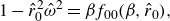 \begin{equation} 1 - \hat {r}_0^2\hat {\omega }^2 = \beta f_{00}(\beta , \hat {r}_0), \end{equation}
where $\hat {r}_0 = k_F r_0$
,
$\hat {r}_0 = k_F r_0$
, $\hat {\omega } = \omega T$
and
$\hat {\omega } = \omega T$
and
 \begin{align} f_{ab}(\eta ,\hat {r}_0) = \pi {\textrm {csch}}(\pi \eta )\frac{\textrm{d}^{a}}{\textrm{d}\hat{r}^{a}_{0}}(\textrm{J}_{-\textrm{i}\eta }(\hat {r}_0))\frac{\textrm{d}^{b}}{\textrm{d}\hat{r}^{b}_{0}}(\textrm{J}_{\textrm{i}\eta }(\hat {r}_0)) \quad \mbox{for } a,b\in \{0,1\}. \end{align}
Furthermore, we define the stability function $\hat {\mathscr{F}}(\hat {s}) = \hat {\mathscr{A}}(\hat {s})\hat {\mathscr{D}}(\hat {s}) + \hat {\mathscr{B}}(\hat {s})\hat {\mathscr{C}}(\hat {s})$
, where
$\hat {\mathscr{F}}(\hat {s}) = \hat {\mathscr{A}}(\hat {s})\hat {\mathscr{D}}(\hat {s}) + \hat {\mathscr{B}}(\hat {s})\hat {\mathscr{C}}(\hat {s})$
, where
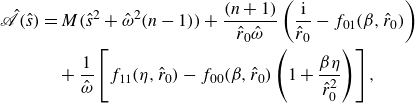 \begin{align} \hat {\mathscr{A}}(\hat {s}) &= M(\hat {s}^2 + \hat {\omega }^2(n-1)) + \frac {(n+1)}{\hat {r}_0\hat {\omega }}\left (\frac {\textrm{i}}{\hat {r}_0} - f_{01}(\beta ,\hat {r}_0)\right )\nonumber \\ &\quad + \frac {1}{\hat {\omega }}\left [f_{11}(\eta ,\hat {r}_0) -f_{00}(\beta ,\hat {r}_0)\left (1 + \frac {\beta \eta }{\hat {r}_0^2}\right )\right ], \end{align}
 \begin{align} \hat {\mathscr{B}}(\hat {s}) = (2-\varDelta )M\hat {\omega }\hat {s} - \frac {\textrm{i}\hat {s}(\varDelta +1)}{\hat {r}_0^2\hat {\omega }^2} + \frac {1}{\hat {r}_0\hat {\omega }}\left [\left (\frac {\hat {s}\Delta }{\hat {\omega }} - \beta \right )f_{01}(\beta ,\hat {r}_0) + \eta f_{01}(\eta ,\hat {r}_0)\right ], \end{align}
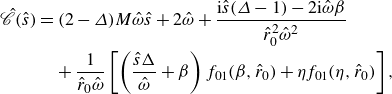 \begin{align} \hat {\mathscr{C}}(\hat {s}) &= (2-\varDelta )M\hat {\omega }\hat {s} + 2\hat {\omega } + \frac {\textrm{i}\hat {s}(\varDelta -1) - 2\textrm{i}\hat {\omega }\beta }{\hat {r}_0^2\hat {\omega }^2}\nonumber\\&\quad + \frac {1}{\hat {r}_0\hat {\omega }}\left [\left (\frac {\hat {s}\Delta }{\hat {\omega }} + \beta \right )f_{01}(\beta ,\hat {r}_0) + \eta f_{01}(\eta ,\hat {r}_0)\right ] , \end{align}
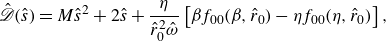 \begin{align} \hat {\mathscr{D}}(\hat {s}) = M\hat {s}^2 + 2\hat {s} + \frac {\eta }{\hat {r}_0^2\hat {\omega }}\left [\beta f_{00}(\beta ,\hat {r}_0) -\eta f_{00}(\eta ,\hat {r}_0)\right ], \end{align} $\hat {s} = sT$
represents the dimensionless complex growth rate,
$\hat {s} = sT$
represents the dimensionless complex growth rate, $\eta = \hat {s}/\hat {\omega } + \beta$
and
$\eta = \hat {s}/\hat {\omega } + \beta$
and $\beta = \zeta /\hat {\omega }$
. Notably,
$\beta = \zeta /\hat {\omega }$
. Notably, $\zeta$
has been eliminated from the stability coefficients by using the tangential force balance (D1a
). We aim to determine the critical value of the reciprocal orbital memory parameter,
$\zeta$
has been eliminated from the stability coefficients by using the tangential force balance (D1a
). We aim to determine the critical value of the reciprocal orbital memory parameter, $\beta$
, at which the growth rate,
$\beta$
, at which the growth rate, $\hat {s}$
, has vanishing real part, writing
$\hat {s}$
, has vanishing real part, writing $\hat {s} = \textrm{i} \xi \hat {\omega }$
for real
$\hat {s} = \textrm{i} \xi \hat {\omega }$
for real $\xi = O(1)$
. We recall that the Coriolis force corresponds to
$\xi = O(1)$
. We recall that the Coriolis force corresponds to $\varDelta = 1$
and
$\varDelta = 1$
and $n = 1$
; the central force corresponds to
$n = 1$
; the central force corresponds to $\varDelta = 0$
with
$\varDelta = 0$
with $n$
being the force power.
$n$
being the force power.
Our analysis hinges on applying asymptotic approximations to the functions $f_{ab}(\beta , \hat {r}_0)$
. The argument of the Bessel function is
$f_{ab}(\beta , \hat {r}_0)$
. The argument of the Bessel function is $\hat {r}_0$
and the complex order is either
$\hat {r}_0$
and the complex order is either $\pm \textrm{i} \eta$
, where
$\pm \textrm{i} \eta$
, where $\eta = \beta + \textrm{i} \xi$
along the stability boundary, or
$\eta = \beta + \textrm{i} \xi$
along the stability boundary, or $\pm \textrm{i} \beta$
. Based on the assumed dominant balances
$\pm \textrm{i} \beta$
. Based on the assumed dominant balances $\beta = O(\ln \hat {r}_0) \ll \sqrt {\hat {r}_0}$
and
$\beta = O(\ln \hat {r}_0) \ll \sqrt {\hat {r}_0}$
and $\xi = O(1)$
, we conclude that the order of the Bessel function is much less than the argument, and thus apply large-argument expansions of Bessel functions (Abramowitz & Stegun Reference Abramowitz and Stegun1948) to the stability problem (D1). The key difference to the Coriolis force problem (Liu et al. Reference Liu, Durey and Bush2023) is that
$\xi = O(1)$
, we conclude that the order of the Bessel function is much less than the argument, and thus apply large-argument expansions of Bessel functions (Abramowitz & Stegun Reference Abramowitz and Stegun1948) to the stability problem (D1). The key difference to the Coriolis force problem (Liu et al. Reference Liu, Durey and Bush2023) is that $\hat {\mathscr{D}}(\textrm{i} \xi \hat {\omega }) = \textrm{i}\xi \hat {\mathscr{C}}(\textrm{i} \xi \hat {\omega }) + \textrm{i}(\varDelta -1) M\hat {\omega }^2\xi + O(\hat {r}_0^{-3})$
, and so terms that vanish for a Coriolis force (
$\hat {\mathscr{D}}(\textrm{i} \xi \hat {\omega }) = \textrm{i}\xi \hat {\mathscr{C}}(\textrm{i} \xi \hat {\omega }) + \textrm{i}(\varDelta -1) M\hat {\omega }^2\xi + O(\hat {r}_0^{-3})$
, and so terms that vanish for a Coriolis force ( $\varDelta = 1$
) are significant for a central force (
$\varDelta = 1$
) are significant for a central force ( $\varDelta = 0$
). We thus require more terms in the expansion of the stability function for a central force. Upon using the tangential equation (D1a
) to eliminate
$\varDelta = 0$
). We thus require more terms in the expansion of the stability function for a central force. Upon using the tangential equation (D1a
) to eliminate $\hat {\omega }$
and approximating
$\hat {\omega }$
and approximating ${\textrm {csch}}(\pi \beta ) = 2\textrm{e}^{-\pi \beta } + O(\textrm{e}^{-2\pi \beta })$
for large
${\textrm {csch}}(\pi \beta ) = 2\textrm{e}^{-\pi \beta } + O(\textrm{e}^{-2\pi \beta })$
for large $\beta$
, we find that the stability function takes the asymptotic form
$\beta$
, we find that the stability function takes the asymptotic form
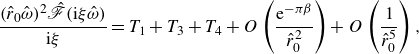 \begin{equation} \frac {(\hat {r}_0\hat {\omega })^2\hat {\mathscr{F}}(\textrm{i} \xi \hat {\omega })}{\textrm{i}\xi } = T_1 + T_3 + T_4 + O\left (\frac {\textrm{e}^{-\pi \beta }}{\hat {r}_0^2}\right ) + O\left (\frac {1}{\hat {r}_0^5}\right ), \end{equation}
where the successive terms, $T_j$
, in the series expansion are
$T_j$
, in the series expansion are
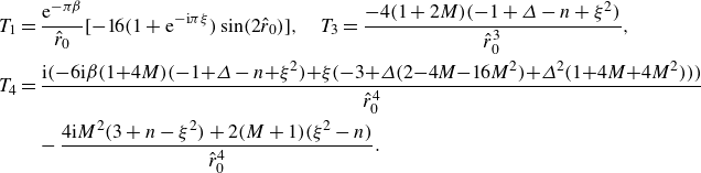 \begin{align} T_1 &= \frac {\textrm{e}^{-\pi \beta }}{\hat {r}_0}[-16(1 + \textrm{e}^{-\textrm{i}\pi \xi })\sin (2\hat {r}_0)], \quad T_3 = \frac {-4(1+2M)(-1+\varDelta -n+\xi ^2)}{\hat {r}_0^3},\nonumber \\ T_4 &= \frac {\textrm{i}(-6\textrm{i}\beta (1\!+\!4M)(-1\!+\!\varDelta -n\!+\!\xi ^2) \!+ \!\xi (-3\!+\!\varDelta (2\!-\!4M\!-\!16M^2) \!+ \!\varDelta ^2(1\!+\!4M\!+\!4M^2)))}{\hat {r}_0^4}\nonumber \\ &\quad- \frac {4\textrm{i} M^2(3+n-\xi ^2) + 2(M+1)(\xi ^2-n)}{\hat {r}_0^4}. \end{align}
Equation (D2) forms the foundation of our analysis of wave- and potential-driven instabilities, where it remains to find asymptotic solutions to $\beta$
and
$\beta$
and $\xi$
satisfying
$\xi$
satisfying $\hat {\mathscr{F}}(\textrm{i} \xi \hat {\omega }) = 0$
for
$\hat {\mathscr{F}}(\textrm{i} \xi \hat {\omega }) = 0$
for $\hat {r}_0 \gg 1$
.
$\hat {r}_0 \gg 1$
.
To proceed, we identify dominant balances between $\textrm{e}^{-\pi \beta }$
and powers of
$\textrm{e}^{-\pi \beta }$
and powers of $\hat {r}_0$
, for which there are two possibilities. If
$\hat {r}_0$
, for which there are two possibilities. If $-1+\varDelta -n+\xi ^2 \neq 0$
, then
$-1+\varDelta -n+\xi ^2 \neq 0$
, then $T_3\neq 0$
and the dominant balance is between terms
$T_3\neq 0$
and the dominant balance is between terms $T_1$
and
$T_1$
and $T_3$
. Otherwise,
$T_3$
. Otherwise, $T_3 = 0$
and so the dominant balance is between terms
$T_3 = 0$
and so the dominant balance is between terms $T_1$
and
$T_1$
and $T_4$
. In the presence of a Coriolis force, for which
$T_4$
. In the presence of a Coriolis force, for which $\varDelta = n = 1$
, we note that
$\varDelta = n = 1$
, we note that $T_3 = 0$
only if
$T_3 = 0$
only if $\xi ^2 = 1$
, which is a trivial eigenvalue corresponding to translational invariance. Thus, for non-trivial eigenvalues, the dominant balance for the Coriolis force system is only ever between terms
$\xi ^2 = 1$
, which is a trivial eigenvalue corresponding to translational invariance. Thus, for non-trivial eigenvalues, the dominant balance for the Coriolis force system is only ever between terms $T_1$
and
$T_1$
and $T_3$
, leading to resonant wave-driven instabilities (Liu et al. Reference Liu, Durey and Bush2023). In contrast, both forms of dominant balance are possible for a central force (
$T_3$
, leading to resonant wave-driven instabilities (Liu et al. Reference Liu, Durey and Bush2023). In contrast, both forms of dominant balance are possible for a central force ( $\varDelta = 0$
), leading to both wave-driven
$\varDelta = 0$
), leading to both wave-driven $(T_3 \neq 0$
) and potential-driven
$(T_3 \neq 0$
) and potential-driven $(T_3 = 0$
) instabilities.
$(T_3 = 0$
) instabilities.
When $T_3 \neq 0$
, the dominant balance between
$T_3 \neq 0$
, the dominant balance between $T_1$
and
$T_1$
and $T_3$
takes the form
$T_3$
takes the form
 \begin{align} -\frac {16\textrm{e}^{-\pi \beta }(1 + \textrm{e}^{-\textrm{i}\pi \xi })\sin (2\hat {r}_0)}{\hat {r}_0} - \frac {4(1+2M)(-1\!+\varDelta -n+\xi ^2)}{\hat {r}_0^3} = O\!\left (\frac {\textrm{e}^{-\pi \beta }}{\hat {r}_0^2}\right ) + \!O\!\left (\frac {1}{\hat {r}_0^4}\right )\!, \end{align}
which we solve for $\beta$
and
$\beta$
and $\xi$
to leading order. Balancing the imaginary parts requires
$\xi$
to leading order. Balancing the imaginary parts requires $\xi$
to be an integer (to leading order), corresponding to resonant wave-driven instabilities. Balancing the real parts requires that integer to be even. The resulting asymptotic solutions for
$\xi$
to be an integer (to leading order), corresponding to resonant wave-driven instabilities. Balancing the real parts requires that integer to be even. The resulting asymptotic solutions for $\beta$
and
$\beta$
and $\xi$
are detailed in (4.1) for a Coriolis force (
$\xi$
are detailed in (4.1) for a Coriolis force ( $\varDelta = n = 1$
) and (4.2) for a central force (
$\varDelta = n = 1$
) and (4.2) for a central force ( $\varDelta = 0$
).
$\varDelta = 0$
).
Potential-driven wobbling instabilities emerge in a central force ( $\varDelta = 0$
) when
$\varDelta = 0$
) when $T_3 = 0$
, corresponding to the leading-order condition
$T_3 = 0$
, corresponding to the leading-order condition $n = \xi ^2 - 1$
, or
$n = \xi ^2 - 1$
, or $\xi = \sqrt {n+1}$
. In this case, the dominant balance between terms
$\xi = \sqrt {n+1}$
. In this case, the dominant balance between terms $T_1$
and
$T_1$
and $T_4$
leads to
$T_4$
leads to
 \begin{align} \!\!\!-\frac {16\textrm{e}^{-\pi \beta }(1+\textrm{e}^{-\textrm{i}\pi \xi })\sin (2\hat {r}_0)}{\hat {r}_0} + \frac {\textrm{i}\xi (4M-1)(2M+1)}{\hat {r}_0^4} = O\left (\frac {\textrm{e}^{-\pi \beta }}{\hat {r}_0^2}\right ) + O\left (\frac {1}{\hat {r}_0^5}\right ). \end{align}
Provided that $\xi = \sqrt {n+1}$
is not an integer, we may use the dominant balance of the imaginary parts to solve for
$\xi = \sqrt {n+1}$
is not an integer, we may use the dominant balance of the imaginary parts to solve for $\beta$
to leading order, which gives rise to the potential-driven wobbling instability boundary detailed in (4.4). When
$\beta$
to leading order, which gives rise to the potential-driven wobbling instability boundary detailed in (4.4). When $\xi = \sqrt {n+1}$
is an integer, potential-driven instabilities are resonant and a more sophisticated asymptotic treatment is necessary.
$\xi = \sqrt {n+1}$
is an integer, potential-driven instabilities are resonant and a more sophisticated asymptotic treatment is necessary.
Appendix E. Instability of small orbits in a sub-linear central force
We proceed to show that $\textrm{d}k_0/\textrm{d}r_0 \gt 0$
for small-radius orbital solutions when
$\textrm{d}k_0/\textrm{d}r_0 \gt 0$
for small-radius orbital solutions when $n\lt 1$
. We then use Theorem1 to conclude that these orbits are unstable to monotonically growing perturbations. For
$n\lt 1$
. We then use Theorem1 to conclude that these orbits are unstable to monotonically growing perturbations. For $k_Fr_0 \ll 1$
, the radial and tangential force balances (3.3) simplify to
$k_Fr_0 \ll 1$
, the radial and tangential force balances (3.3) simplify to
 \begin{align} -mr_0\omega ^2 = \frac {Fk_F r_0\omega ^2 T_M}{2T_F(\omega ^2 + T_M^{-2})} - kr_0^n + O(r_0^3), \qquad D = \frac {Fk_F}{2T_F(\omega ^2 + T_M^{-2})} + O(r_0^2), \end{align}
respectively. Along the orbital solution curve, $\omega = \omega _0(r_0)$
and
$\omega = \omega _0(r_0)$
and $k = k_0(r_0)$
are thus
$k = k_0(r_0)$
are thus
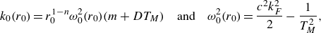 \begin{align} k_0(r_0) = r_0^{1-n}\omega _0^2(r_0)(m + DT_M) \quad \mbox{and}\quad \omega _0^2(r_0) = \frac {c^2 k_F^2}{2} - \frac {1}{T_M^2}, \end{align}
where $c = \sqrt {F/DT_F k_F}$
is the maximum orbital speed. Notably, the orbital frequency,
$c = \sqrt {F/DT_F k_F}$
is the maximum orbital speed. Notably, the orbital frequency, $\omega _0(r_0)$
, for small circular orbits is the same as for a rotating frame (Oza et al. Reference Oza, Harris, Rosales and Bush2014a
), and is valid provided that
$\omega _0(r_0)$
, for small circular orbits is the same as for a rotating frame (Oza et al. Reference Oza, Harris, Rosales and Bush2014a
), and is valid provided that $T_M \gt T_W$
, where
$T_M \gt T_W$
, where $T_W = \sqrt {2}/ck_F$
is the memory time at the walking threshold (Durey et al. Reference Durey, Turton and Bush2020b
). As
$T_W = \sqrt {2}/ck_F$
is the memory time at the walking threshold (Durey et al. Reference Durey, Turton and Bush2020b
). As $\omega _0(r_0)$
is independent of
$\omega _0(r_0)$
is independent of $r_0$
to leading order, we deduce that
$r_0$
to leading order, we deduce that
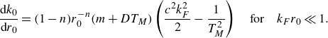 \begin{align} \frac {\textrm{d} {k_0}}{\textrm{d}{r_0}} = (1-n)r_0^{-n}(m+DT_M)\left (\frac {c^2k_F^2}{2} - \frac {1}{T_M^2}\right ) \quad \mbox{for}\quad k_F r_0 \ll 1. \end{align}
We thus conclude that $\textrm{d}k_0/\textrm{d}r_0 \gt 0$
for sufficiently small orbital radii when
$\textrm{d}k_0/\textrm{d}r_0 \gt 0$
for sufficiently small orbital radii when $n \lt 1$
(with
$n \lt 1$
(with $T_M \gt T_W$
), with orbits destabilising via monotonically growing perturbations.
$T_M \gt T_W$
), with orbits destabilising via monotonically growing perturbations.
Appendix F. Proof that $\pmb{\mathscr{D}}'(\textbf{0}) \boldsymbol{\gt} \textbf{0}$
for the stroboscopic model
$\pmb{\mathscr{D}}'(\textbf{0}) \boldsymbol{\gt} \textbf{0}$
for the stroboscopic model

To prove that $\mathscr{D}'(0) \gt 0$
for the stroboscopic pilot-wave model, with
$\mathscr{D}'(0) \gt 0$
for the stroboscopic pilot-wave model, with $\mathscr{D}(s)$
defined in (C1d
), we first convert to dimensionless variables. As outlined in Appendix D, we define
$\mathscr{D}(s)$
defined in (C1d
), we first convert to dimensionless variables. As outlined in Appendix D, we define $\hat {\mathscr{D}}(\hat {s}) = \mathscr{D}(s)T/D$
, where
$\hat {\mathscr{D}}(\hat {s}) = \mathscr{D}(s)T/D$
, where $\hat {s} = sT$
and
$\hat {s} = sT$
and $T = 1/(c k_F)$
is the unit of time. From (D1e
), it thus remains to prove that
$T = 1/(c k_F)$
is the unit of time. From (D1e
), it thus remains to prove that $\hat {\mathscr{D}}'(0) \gt 0$
, where
$\hat {\mathscr{D}}'(0) \gt 0$
, where
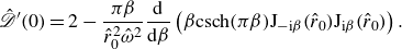 \begin{gather} \hat {\mathscr{D}}'(0) = 2 - \frac {\pi \beta }{\hat {r}_0^2\hat {\omega }^2}\frac {\textrm{d} {}}{\textrm{d}{\beta }}\left (\beta {\textrm {csch}}(\pi \beta )\textrm{J}_{-\textrm{i}\beta}(\hat {r}_0)\textrm{J}_{\textrm{i}\beta}(\hat {r}_0)\right). \end{gather}
To proceed, we express the product in parentheses in (F1) in terms of an infinite sum, which is achieved by combining (C4a
) and (C4b
) with $m = 0$
to give
$m = 0$
to give
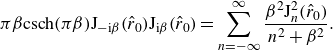 \begin{gather} \pi \beta {\textrm {csch}}(\pi \beta )\textrm{J}_{-\textrm{i}\beta }(\hat {r}_0)\textrm{J}_{\textrm{i}\beta }(\hat {r}_0) = \sum _{n=-\infty }^\infty \frac {\beta ^2\textrm{J}_n^2(\hat {r}_0)}{n^2+\beta ^2}. \end{gather}
Substituting (F2) into (F1) and differentiating the sum term by term yields
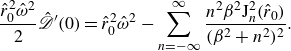 \begin{equation} \frac {\hat {r}_0^2\hat {\omega }^2}{2}\hat {\mathscr{D}}'(0) = \hat {r}_0^2\hat {\omega }^2 - \sum _{n=-\infty }^\infty \frac {n^2\beta ^2 \textrm{J}_n^2(\hat {r}_0)}{(\beta ^2 + n^2)^2}. \end{equation}
We now recognise that the left-hand side of (F2) is the same as the right-hand side of the tangential force balance (D1a
). We may thus express the tangential force balance in terms of the infinite sum in (F2) and then eliminate $\hat {r}_0^2\hat {\omega }^2$
from the right-hand side of (F3). A short calculation gives rise to the expression
$\hat {r}_0^2\hat {\omega }^2$
from the right-hand side of (F3). A short calculation gives rise to the expression
 \begin{gather} \frac {\hat {r}_0^2\hat {\omega }^2}{2}\hat {\mathscr{D}}'(0) = 1 - \sum _{n=-\infty }^\infty \frac {\textrm{J}_n^2(\hat {r}_0)\beta ^2}{(\beta ^2+n^2)}\left (1 + \frac {n^2}{\beta ^2+n^2}\right ) = \sum _{n=-\infty }^\infty \frac {n^4 \textrm{J}_n^2(\hat {r}_0)}{(\beta ^2 + n^2)^2}, \end{gather}
where the right-hand side has been simplified using the identity $\sum _{n=-\infty }^\infty \textrm{J}_n^2(\hat {r}_0) = 1$
. As all terms in the final sum in (F4) are either zero or positive, we conclude that
$\sum _{n=-\infty }^\infty \textrm{J}_n^2(\hat {r}_0) = 1$
. As all terms in the final sum in (F4) are either zero or positive, we conclude that $\hat {\mathscr{D}}'(0) \gt 0$
, and thus
$\hat {\mathscr{D}}'(0) \gt 0$
, and thus $\mathscr{D}'(0) \gt 0$
for the stroboscopic pilot-wave model.
$\mathscr{D}'(0) \gt 0$
for the stroboscopic pilot-wave model.


 Open access