Axisymmetric dynamos sustained by a modified Ohm’s law in a toroidal volume

Abstract

This work tackles a significant challenge in dynamo theory: the possibility of long-term amplification and maintenance of an axisymmetric magnetic field. We introduce a novel model that allows for non-trivial axially symmetric steady-state solutions for the magnetic field, particularly when the dynamo operates primarily within a ‘nearly spherical’ toroidal volume inside a fluid shell surrounding a solid core. In this model, Ohm’s law is generalised to include the dissipative force, arising from electron collisions, that tends to align the velocity of the shell with the rotational speed of the inner core and outer mantle. Our findings reveal that, in this context, Cowling’s theorem and the neutral point argument are modified, leading to magnetic energy growth for a suitable choice of toroidal flow. The global equilibrium magnetic field that emerges from our model exhibits a dipolar character. The central insight of the model developed here is that if an additional force is incorporated into Ohm’s law, symmetric dynamos become possible.

1. Introduction

Dynamo theory posits that planetary and stellar magnetic fields are generated by converting kinetic energy into magnetic energy via Faraday’s law of induction in a magnetohydrodynamic (MHD) fluid (e.g. Moffatt 1978; Desjardins et al. 2007; Tobias 2021). The mechanism behind the long-term amplification and maintenance of these fields, particularly axisymmetric magnetic fields, remains a longstanding theoretical problem. This inquiry dates back to Larmor (1919), who hypothesised that a flow of ionised gas (as in the Sun) occurring in a magnetic field aligned with an axis would induce a toroidal electric current circulating about the axis, thereby sequentially enhancing the magnetic field. However, Cowling’s neutral point argument (Cowling 1933) established the well-known antidynamo theorem, stating that an axisymmetric magnetic field cannot be sustained by dynamo action. This finding laid the groundwork for mean-field theory (e.g. Krause & Rädler 1980) and nearly axisymmetric dynamos (Braginsky 1976), while kinematic approaches explored magnetic field enhancement through predefined velocity fields (e.g. Backus 1958; Ponomarenko 1973). Meanwhile, theoretical efforts aimed to generalise Cowling’s theorem by removing the restrictions noted in his original proof and possibly finding ways to circumvent it (see detailed discussions in Ivers & James (1984), Núñez (1996) and Kaiser & Tilgner (2014)). Allowing anisotropy in conductivity emerged as a potential solution to support symmetric field configurations (Lortz 1989; Plunian & Alboussière 2020). Interestingly, modelling compressibility and/or variable conductivity in gaseous planets, spherical MHD dynamo simulations exhibited quasi-equilibrium fields that were almost-axisymmetric and dipole-dominated (Nishikawa & Kusano 2008; Yadav, Cao & Bloxham 2022).

In this study, we revisit the fundamental question of whether axisymmetric dynamos can be theoretically realised within the framework of kinematic dynamo theory. Here, an axisymmetric dynamo refers to the spontaneous generation of a magnetic field that exhibits axial symmetry. Our hypothesis is that the dissipative force arising from electron–electron collisions – commonly neglected in standard MHD – may play a role in geophysical and astrophysical dynamos. We highlight that this MHD regime serves as a simplified model for certain planetary or stellar interiors, as such systems – whether consisting of fully ionised plasma or liquid metal – can be effectively modelled as a two-fluid system of ions and electrons interacting through electromagnetic forces. The dissipative force due to electron–electron collisions becomes particularly significant when the turbulence scale of the fluid flow in planetary/stellar interiors is sufficiently small, thereby requiring a modification to Ohm’s law. Indeed, the constitutive relation connecting the electric field to the magnetic field and velocity field depends on the forces acting on the electron fluid (Freidberg 2014). To explore this idea, we propose two simplified models for the dissipative force: a restoring friction force model and a viscous dissipation model. Importantly, the emphasis of this work lies in the underlying physical principle: if an additional force is incorporated into Ohm’s law, symmetric dynamos become possible.

In fusion plasma physics, stable equilibrium magnetic fields are crucial for developing magnetic confinement fusion reactors (Wesson 2004; Helander 2014). A key property of fusion reactors is that they must be toroidal rather than spherical, due to the impossibility of accommodating a non-vanishing magnetic field on a spherical surface (hairy ball theorem; Eisenberg & Guy 1979). This work builds on these principles by modelling a planetary/stellar dynamo-active region, situated between an inner core and an outer mantle, as a ‘nearly spherical’ thick toroidal volume enclosed within a spherical fluid shell. This volume resembles the shape formed when attempting to fit a torus into a hollow sphere (see § 2 and figure 1). Applying the modified Ohm’s law that accounts for the dissipative force caused by electron collisions, we show that the resulting dynamo model successfully generates an axially symmetric dipolar magnetic field driven by an ion flow aligned with the steady electric current density. We also uncover that, at equilibrium, the ideal convective (Lorentz) forces and the dissipative (Ohmic resistance and friction/viscosity) forces balance independently. This regime aligns with the kinetic theory of plasmas (e.g. Sato & Morrison 2024), from which MHD originates.

The present model may thus serve as an illustrative example for understanding the dynamo mechanism responsible for generating the dominant dipole component of planetary and stellar magnetic fields, including the highly symmetric configurations observed in Saturn and Mercury (e.g. Anderson et al. 2012; Cao et al. 2023). The nearly axisymmetric fields of the gas giant and the rocky planet have been attributed to the influence of a stably stratified layer above the dynamo region (Stevenson 1980; Christensen 2006). Our model suggests that this can naturally result from dynamo action confined within a toroidal volume inside the spherical dynamo region, influenced by the balance of resistive and friction/viscosity forces.

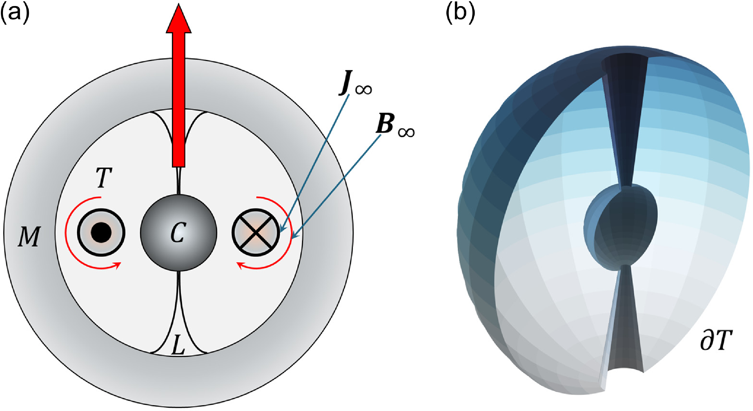
Figure 1. (a) Schematic representation of a dynamo region in a planet. Note that the current density $\boldsymbol{J}_{\infty }$ responsible for the dipole magnetic field $\boldsymbol{B}_{\infty }$ flows within a toroidal volume $T$ entirely contained within the fluid shell $L$ . (b) Half-cut toroidal surface $\partial T$ bounding the toroidal dynamo region $T$ . Note that the current density $ \boldsymbol{J}_{\infty }$ vanishes in the dark region surrounding the vertical axis, which corresponds to the toroidal hole.

2. Modelling an internal dynamo region

In this section, we introduce a simplified model of the interior regions beneath the surface of a planet with volume $ S \subset \mathbb{R}^3$ . Specifically, we model the dynamo-active region $ T$ – the region where the electric current density responsible for dynamo action is non-vanishing – as a toroidal volume $ T \subset S$ .

The choice of a toroidal volume is motivated by the nature of axially symmetric dipole magnetic fields generated by spontaneous dynamo action. In such cases, the corresponding electric current density is toroidal and can be expressed as $ \boldsymbol{J} = \alpha (r,z)\nabla \varphi$ , where $ (r,\varphi ,z)$ are cylindrical coordinates, and $ \alpha (r,z)$ is a function of $ r$ and $ z$ . Due to the singularity of $ |\nabla \varphi | = 1/r$ at $ r=0$ , and the fact that the direction of $\nabla \varphi$ is not uniquely defined at $r=0$ , the current density $ \boldsymbol{J}$ must vanish along the planetary axis ( $ r=0$ ). Consequently, a dynamo-active region sustaining such an an axially symmetric magnetic field cannot have a spherical topology. Instead, it can be appropriately modelled as a toroidal volume $ T \subset S$ embedded within the planetary volume $ S \subset \mathbb{R}^3$ .

This observation is closely related to the Poincaré–Hopf and hairy ball theorems (Eisenberg & Guy 1979), which state that a non-vanishing continuous vector field cannot exist tangent to a spherical surface. For a sphere to accommodate a toroidal current, there must be regions where the current vanishes. Practically, this implies the absence of significant macroscopic currents near the planet’s poles, supporting the choice of a topologically toroidal dynamo-active region.

We further assume that the magnetic axis aligns approximately with the planet’s rotational axis and that $ T$ exhibits rotational symmetry around the vertical axis connecting the poles. The planetary structure is modelled with a solid core $ C$ , surrounded by a fluid shell $ L$ , which lies beneath the mantle $ M$ . Here, $ C$ is a spherical volume, while $ L$ and $ M$ are hollow spherical shells. Both the solid core and fluid shell may be electrically conducting; however, the solid nature of the core suggests that convective currents sustaining the planet’s magnetic field are confined to the fluid shell. Hence, $ T \subset L$ .

Additionally, we assume that the toroidal volume $ T$ nearly fills the fluid shell $ L$ , resulting in a ‘nearly spherical’ yet topologically toroidal region (see figure 1). For the purposes of this study, we focus on $ T$ and the exterior region $ O = \mathbb{R}^3 \setminus \bar {T}$ , where $ \bar {T}$ denotes the closure of $ T$ .

A schematic representation of this model is shown in figure 1. In this figure, $ \boldsymbol{J}_{\infty }(\boldsymbol{x}) = \mu _0^{-1} \unicode{x1D6FB} \times \boldsymbol{B}_{\infty }(\boldsymbol{x})$ and $ \boldsymbol{B}_{\infty }(\boldsymbol{x})$ denote the long-term current density and magnetic field, respectively, representing the final equilibrium fields resulting from dynamo action. Here, $ \mu _0$ is the vacuum permeability.

3. Modified Ohm’s law incorporating electron collisions

In the following, we adopt a simplified model of the electrically conducting fluid responsible for dynamo action, described as an ion–electron two-fluid system. This simplified approach is not intended for making quantitative predictions about the magnetic properties of specific planets or stars. Instead, it provides a conceptual framework that highlights the core physical principle: if an additional force is incorporated into Ohm’s law, symmetric dynamos become possible.

Ohm’s law relates the electric field $\boldsymbol{E}({\boldsymbol{x},t})$ to the velocity field $\boldsymbol{u}({\boldsymbol{x},t})$ , the magnetic field $\boldsymbol{B}({\boldsymbol{x},t})$ and the current density $\boldsymbol{J}({\boldsymbol{x},t})$ through the resistivity $\eta \gt 0$ , modelled as a constant, according to

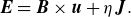(3.1) \begin{equation} \begin{split} \boldsymbol{E}=\boldsymbol{B}\times \boldsymbol{u}+\eta \boldsymbol{J}. \end{split} \end{equation}

Equation (3.1) originates from the electron fluid momentum equation

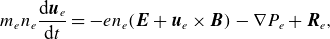(3.2) \begin{equation} \begin{split} m_en_e\frac {{\rm d}\boldsymbol{u}_e}{{\rm d}t}=-en_e({\boldsymbol{E}+\boldsymbol{u}_e\times \boldsymbol{B}})-\nabla P_e+\boldsymbol{R}_e, \end{split} \end{equation}

where $m_e$ , $-e$ , $n_e({\boldsymbol{x},t})$ , $\boldsymbol{u}_e({\boldsymbol{x},t})$ , $P_e({\boldsymbol{x},t})$ and $\boldsymbol{R}_e({\boldsymbol{x},t})$ denote the electron mass, charge, number density, fluid velocity, pressure and resistive force resulting from ion–electron collisions, respectively (Freidberg 2014). Recalling that the electron fluid velocity $\boldsymbol{u}_e$ is related to the current density $\boldsymbol{J}$ , the ion fluid velocity $\boldsymbol{u}_i({\boldsymbol{x},t})$ , the ion number density $n_i({\boldsymbol{x},t})$ and the ion charge $Ze$ according to $ \boldsymbol{J}=e({Zn_i\boldsymbol{u}_i-n_e\boldsymbol{u}_e})$ , (3.2) can be solved for $\boldsymbol{E}$ . Due to the smallness of the electron to ion mass ratio $\delta =m_e/m_i$ , the velocity of the centre of mass of the ion–electron two-fluid system effectively corresponds to the ion fluid velocity, i.e. $\boldsymbol{u}= ({\boldsymbol{u}_i+\delta \boldsymbol{u}_e})/({1+\delta })\approx \boldsymbol{u}_i$ . Furthermore, assuming quasi-neutrality, we have $n({\boldsymbol{x},t}) =n_i\approx n_e/Z$ , leading to

(3.3) \begin{equation} \begin{split} \boldsymbol{E}=\boldsymbol{B}\times \boldsymbol{u}+\frac {1}{Ze n}\boldsymbol{J}\times \boldsymbol{B}-\frac {1}{Zen}\nabla P_e+\frac {\boldsymbol{R}_e}{Zen}-\frac {m_e}{e}\frac {{\rm d}\boldsymbol{u}_e}{{\rm d}t}. \end{split} \end{equation}

The second term on the right-hand side is the Hall effect. In the regime of MHD, both the Hall and electron pressure terms (3.3) scale with the ion-gyroradius, and are therefore neglected on the larger spatial scale of the system. The last term on the right-hand side of (3.3) is similarly neglected under the standard MHD assumption (Freidberg 2014) that the small electron mass makes it smaller than all the other terms, including the resistive term $\boldsymbol{R}_e/Zen$ . If we further assume a linearity relationship between $\boldsymbol{R}_e$ and the current density $\boldsymbol{J}$ , i.e.

(3.4) \begin{equation} \begin{split} \frac {\boldsymbol{R}_{e}}{Zen}=\eta \boldsymbol{J}, \end{split} \end{equation}

we arrive at Ohm’s law (3.1). For completeness, it is important to note that the derivation of Ohm’s law presented previously aligns well with the classical Drude model (Ashcroft & Mermin 1976), which describes electrons as following random trajectories due to collisions with stationary ions. The emergence of a steady-state characterised by a linear response to the applied electric field is intrinsically tied to the small mass of the electron. This small mass enables an exceptionally fast response time relative to the MHD time scale, thereby ensuring that the system quickly reaches equilibrium where the current density is proportional to the electric field.

The standard form of Ohm’s law (3.1) is valid only within the parameter regime of MHD. However, it is well established that Ohm’s law must be modified when the assumptions underlying this regime no longer hold. For a detailed discussion on the applicability of MHD, we refer to Freidberg (2014) and Fitzpatrick (2015). Generalised forms of Ohm’s law, such as those in Hall MHD (Acheritogaray et al. 2011) and extended MHD (Abdelhamid, Kawazura & Yoshida 2015), have been employed in applications to dynamo theory (Minnini, Gómez & Mahajan 2003; Lingam & Mahajan 2015). The central idea of this study is that the dissipative force arising from electron–electron collisions, which is typically neglected in standard MHD, may play a significant role in geophysical and astrophysical dynamos. This necessitates a corresponding modification of Ohm’s law (3.1). In the remainder of this section, we develop a model for this modified form of Ohm’s law.

Now suppose that we move to a rotating reference frame with speed $\boldsymbol{v}_{\!R}= ({1}/{2})\varOmega r^2\nabla \varphi$ , where $\varOmega \gt 0$ is a constant and $({r,\varphi ,z})$ is a cylindrical coordinate system. In the rotating frame, the ion and electron fluid velocities become $\boldsymbol{u}'=\boldsymbol{u}-\boldsymbol{v}_{\!R}$ and $\boldsymbol{u}_e'=\boldsymbol{u}_e-\boldsymbol{v}_{\!R}$ . It follows that

(3.5) \begin{equation} \begin{split} \boldsymbol{J}=Ze n\left ({\boldsymbol{u}-\boldsymbol{u}_e}\right )=Zen({\boldsymbol{u}'-\boldsymbol{u}_e'})=\boldsymbol{J}', \end{split} \end{equation}

where the prime means that the quantity is evaluated in the rotating frame. Equations (3.4) and (3.5) show that the resistive force $\boldsymbol{R}_e$ cannot take into account dissipative forces that cannot be expressed through the relative velocity $\boldsymbol{u}-\boldsymbol{u}_e$ . Indeed, the force $\boldsymbol{R}_e$ does not change in the presence of rotation $\boldsymbol{v}_{\!R}$ due to the invariance of $\boldsymbol{J}$ described by (3.5). However, the fluid shell surrounding the solid core cannot slide: it is subject to friction forces that tend to make uniform the speed of the fluid with the rotation speed $\boldsymbol{v}_{\!R}$ of the inner core and the overlying mantle. Now imagine sliding a condensed viscous fluid on a rough surface. It is then unlikely that these friction forces can be neglected in the modelling of the fluid shell. The simplest model for this type of friction is given by a restoring force $\boldsymbol{F}_{\!\gamma }$ acting on the electron fluid

(3.6) \begin{equation} \begin{split} \boldsymbol{F}_{\!\gamma }=-Ze\gamma n({\boldsymbol{u}_e-\boldsymbol{v}_{\!R}})=-Ze\gamma n({\boldsymbol{u}-\boldsymbol{v}_{\!R}})+\gamma \boldsymbol{J}, \end{split} \end{equation}

where $\gamma \gt 0$ is a physical constant. The result is a modified Ohm’s law,

(3.7) \begin{equation} \begin{split} \boldsymbol{E}= \boldsymbol{B}\times \boldsymbol{u}+\eta _{\gamma }\boldsymbol{J}-\gamma ({\boldsymbol{u}-\boldsymbol{v}_{\!R}}),\,\,\,\,\eta _\gamma =\eta + ({\gamma }/{Zen}). \end{split} \end{equation}

Note that we introduced an effective resistivity $\eta _{\gamma }$ . Remarkably, the restoring force contains a toroidal component $({\boldsymbol{u}-\boldsymbol{v}_{\!R}})\cdot \nabla \varphi$ that can potentially balance a toroidal current density $\boldsymbol{J}\cdot \nabla \varphi \neq 0$ . Indeed, the difference $\boldsymbol{u}-\boldsymbol{u}_e$ between ion fluid velocity and electron fluid velocity can have the same orientation as the difference $\boldsymbol{u}_e-\boldsymbol{v}_{\!R}$ between electron fluid velocity and rotation velocity, implying that the resistive force $\eta \boldsymbol{J}$ can be balanced by the restoring force $-\gamma ({\boldsymbol{u}_e-\boldsymbol{v}_{\!R}})$ . Physically, the fast moving ions attract the electron fluid in one direction, while rotation of the planet effectively drags them in the other.

It is worth noting that the resistive force, which is proportional to $\boldsymbol{u} - \boldsymbol{u}_e$ , and the frictional force, which is proportional to $\boldsymbol{u} - \boldsymbol{v}_{\!R}$ , share the same mathematical structure. In the case of the resistive force, this structure represents the linear response to electron–ion collisions. Conversely, the frictional force models the linear response to electron–electron collisions, which interact with the rotating inner core and outer mantle as they collide with the boundary of the toroidal domain, propagating this effect through subsequent collisions. We also remark that the friction force $\boldsymbol{F}_{\!\gamma }$ is consistent with Galilean invariance, as the velocity differences $\boldsymbol{u} - \boldsymbol{v}_{\!R}$ and $\boldsymbol{u} - \boldsymbol{u}_e$ remain invariant across inertial frames under Galilean relativity.

We emphasise that (3.6) represents a simplified description of the actual friction force at play in the fluid shell, and is chosen to simplify the later analysis. This friction force is ultimately rooted in the momentum transfer associated with electron collisions. An accurate derivation of the friction force should take into account the individual condition of the planet, e.g. the graduality of the transition from liquid to solid phase in Earth’s interior, and would require kinetic modelling of particle collisions in a rotating setting, leading to a corresponding electron fluid momentum equation subject to boundary conditions for the velocity field that take into account the planet’s rotation. If viscous resistive MHD equations are chosen to model the electron momentum equation in the rotating frame, the resulting modification of Ohm’s law in the non-rotating rest frame is

(3.8) \begin{equation} \begin{split} \boldsymbol{E}=\boldsymbol{B}\times \boldsymbol{u}+\eta \boldsymbol{J}+ (({m_e\nu _e})/{e})\Delta \boldsymbol{u}_e\approx \boldsymbol{B}\times \boldsymbol{u}+\eta \boldsymbol{J}+ (({m_e\nu _e})/{e})\Delta \boldsymbol{u}, \end{split} \end{equation}

where $\nu _e$ is the electron fluid kinematic viscosity, $\Delta$ the Laplacian operator, we used the fact that $\Delta \boldsymbol{v}_{\!R}=\boldsymbol{0}$ and neglected the term proportional to $\Delta ({\boldsymbol{J}/Zen})$ , which is expected to represent a higher order correction in the plasma regime under consideration. Note that, although $\boldsymbol{v}_{\!R}$ does not appear explicitly in $\Delta \boldsymbol{u}$ , the presence of the operator $\Delta$ implies that planetary rotation is felt throughout the toroidal domain via the no-slip boundary conditions on $\boldsymbol{u}$ .

It is important to note that since the difference $\boldsymbol{u} - \boldsymbol{u}_e$ can be small relative to $\boldsymbol{u}$ , the viscous term may be comparable to the resistive term. This implies that neglecting viscous effects in resistive MHD may not always be a valid approximation, as clear from the numerical examples given below. In particular, note that when approaching the boundary of the fluid shell, the current density progressively drops towards zero, leaving the friction/viscous forces the dominant toroidal component in Ohm’s law. In fact, the condition $\eta \boldsymbol{J}\sim m_e\nu _e\Delta \boldsymbol{u}/e$ can be used to estimate the characteristic spatial scale $L$ of the relative velocity $\boldsymbol{u}-\boldsymbol{v}_{\!R}$ in the fluid shell needed to sustain a given current density $\boldsymbol{J}$ . We have

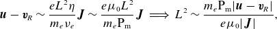(3.9) \begin{equation} \boldsymbol{u}-\boldsymbol{v}_{\!R}\sim \frac {eL^2\eta }{m_e\nu _e}\boldsymbol{J}\sim \frac {e\mu _0L^2}{m_e\mathrm{P_m}}\boldsymbol{J} \implies L^2\sim \frac {m_e\mathrm{P_m}\lvert {\boldsymbol{u}-\boldsymbol{v}_{\!R}}\rvert }{e\mu _0\lvert {\boldsymbol{J}}\rvert }, \end{equation}

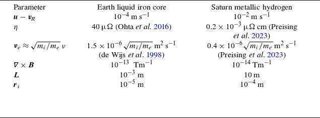
where $\mathrm{P_m}=\mu _0\nu _e/\eta$ is the (electron) magnetic Prandtl number. For given $\boldsymbol{u}-\boldsymbol{v}_{\!R}$ , we see that when $\mathrm{P_m}$ is smaller, the current density and the turbulence scale $L$ tend to be very small. Conversely, in areas where $\mathrm{P_m}$ is higher, substantial currents can flow and larger scales $L$ are allowed. As an example, consider Earth’s liquid iron core for a relative velocity of $\boldsymbol{u} - \boldsymbol{v}_{\!R} \approx 10^{-4} \, \text {m s}^{-1}$ . Using estimated values for resistivity, $\eta \approx 40 \, \unicode{x03BC} \varOmega \,\text{cm}$ (Ohta et al. 2016), and kinematic viscosity, $\nu \approx 1.5\times 10^{-6} \, \text{m}^2\,\rm s^{-1}$ (de Wijs et al. 1998), noting that $\nu _e\approx \sqrt {{m_i}/{m_e}}\nu$ (Freidberg 2014), one finds a turbulence scale of $L \approx 10^{-3}\,\text{m}$ for the geomagnetic field $\boldsymbol{B} \approx 10^{-6} \, \text{T}$ such that $\unicode{x1D6FB} \times \boldsymbol{B} \approx 10^{-13} \, \rm T\, m^{-1}$ . A similar estimate for Saturn’s metallic hydrogen, with $\nu \approx 0.4\times 10^{-6}\mathrm{m}^2\,\rm s^{-1}$ , $\eta \approx 0.2\times 10^{-3} \unicode{x03BC}\Omega \,\text{cm}$ (Preising et al. 2023) and $\unicode{x1D6FB} \times \boldsymbol{B}\approx 10^{-14}\,\rm T\, m^{-1}$ , gives $L\approx 10\,\text{m}$ when $\boldsymbol{u}-\boldsymbol{v}_{\!R}\approx 10^{-2}\,\text{ m s}^{-1}$ . In those plasma regimes, by contrast, the ion gyroradii $r_{i}$ are found to be approximately $ 10^{-5} \, \text{m}$ and $10^{-4}\,\text{m}$ for the Earth and Saturn, respectively. The MHD approximation with the modified Ohm’s law is hence valid here (see table 1). We also note that these estimates on $L$ likely represent lower bounds as $\nu _e\approx \sqrt {m_i/m_e}\nu$ only takes into account electron–electron collisions.

Finally, we remark that similar considerations apply to the ratio of the friction force $\boldsymbol{F}_{\!\gamma }$ and the resistive term $\eta \boldsymbol{J}$ , as $\boldsymbol{F}_{\!\gamma }$ and $\Delta \boldsymbol{u}$ model the same dissipative force.

Table 1. Comparison of parameters for Earth’s liquid iron core and Saturn’s metallic hydrogen. $L$ is the spatial turbulence scale at which the resistive term $\eta \boldsymbol{J}$ is comparable to the viscous term $m_e\nu _e\Delta \boldsymbol{u}/e$ .

4. Modified Cowling’s theorem

Let us examine how Cowling’s theorem changes under the modified Ohm’s law (3.7). It will be sufficient to consider an axially symmetric poloidal magnetic field

(4.1) \begin{equation} \begin{split} \boldsymbol{B}=\nabla \varPsi \times \nabla \varphi , \end{split} \end{equation}

where $\varPsi ({r,z,t})$ denotes the flux function, and an axially symmetric velocity field

(4.2) \begin{equation} \begin{split} \boldsymbol{u}=\nabla \varTheta \times \nabla \varphi +g\nabla \varphi , \end{split} \end{equation}

with $\varTheta ({r,z,t})$ and $g({r,z,t})$ single-valued functions. For simplicity, we hereafter assume $\eta _{\gamma }\gt 0$ to be constant. Using (3.7), the induction equation for the magnetic field $\boldsymbol{B}$ reads as

(4.3) \begin{equation} \begin{split} \frac {\partial \boldsymbol{B}}{\partial t}=\unicode{x1D6FB} \times \left ({\boldsymbol{u}\times \boldsymbol{B}-\eta _{\gamma }\boldsymbol{J}+\gamma \boldsymbol{u}}\right )-\gamma \varOmega \nabla z. \end{split} \end{equation}

Substituting (4.1), we have

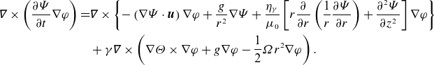(4.4) \begin{align} \unicode{x1D6FB} \times \left ({\frac {\partial \varPsi }{\partial t}\nabla \varphi }\right )=&\unicode{x1D6FB} \times \left \{{-\left ({\nabla \varPsi \cdot \boldsymbol{u}}\right )\nabla \varphi +\frac {g}{r^2}\nabla \varPsi +\frac {\eta _{\gamma }}{\mu _0}\left [{r\frac {\partial }{\partial r}\left ({\frac {1}{r}\frac {\partial \varPsi }{\partial r}}\right )+\frac {\partial ^2\varPsi }{\partial z^2}}\right ]\nabla \varphi }\right \}\nonumber\\ &+\gamma \unicode{x1D6FB} \times \left ({\nabla \varTheta \times \nabla \varphi +g\nabla \varphi -\frac {1}{2}\varOmega r^2\nabla \varphi }\right ). \end{align}

Considering a toroidal volume $T\subset \mathbb{R}^3$ as domain for the induction equation, we can remove the curl operator by introducing a potential $\varPhi ({r,z,t})$ such that

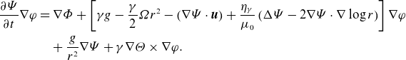(4.5) \begin{align} \frac {\partial \varPsi }{\partial t}\nabla \varphi & = \nabla \varPhi +\left [{\gamma g-\frac {\gamma }{2}\varOmega r^2-\left ({\nabla \varPsi \cdot \boldsymbol{u}}\right )+\frac {\eta _{\gamma }}{\mu _0}\left ({ \Delta \varPsi -2\nabla \varPsi \cdot \nabla \log r }\right )}\right ]\nabla \varphi \nonumber\\& \quad +\frac {g}{r^2}\nabla \varPsi +\gamma \nabla \varTheta \times \nabla \varphi . \end{align}

The toroidal component of this equation reads as

(4.6) \begin{equation} \begin{split} \frac {\partial \varPsi }{\partial t}= \gamma g-\frac {\gamma }{2}\varOmega r^2-{\nabla \varPsi \cdot \boldsymbol{u}}+\frac {\eta _{\gamma }}{\mu _0} \left ({\Delta \varPsi -2\nabla \varPsi \cdot \nabla \log r}\right ). \end{split} \end{equation}

A key observation is that this governing equation allows for a zero magnetic field solution whenever the toroidal velocity equals the planet’s rotational speed, specifically when $ g = {\varOmega r^2}/{2}$ . Hence, the system is not frictionally driven, allowing for spontaneous dynamo action.

Next, we evaluate the integral

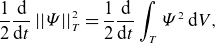(4.7) \begin{equation} \begin{split} \frac {1}{2}\frac {\rm d}{{\rm d}t}\left \lvert \left \lvert \varPsi \right \rvert \right \rvert _{T}^2=\frac {1}{2}\frac {\rm d}{{\rm d}t} \int _{T}\varPsi ^2\,{\rm d}V, \end{split} \end{equation}

where $\lvert \lvert \cdot \rvert \rvert _{T}$ denotes the standard $L^2({T})$ norm. We have

(4.8) \begin{equation} \begin{split} \frac {1}{2}&\frac {\rm d}{{\rm d}t}\left \lvert \left \lvert \varPsi \right \rvert \right \rvert _{T}^2=\int _{T}\varPsi \left [{\gamma g-\frac {\gamma }{2}\varOmega r^2-\nabla \varPsi \cdot \boldsymbol{u}+\frac {\eta _{\gamma }}{\mu _0}\left ({\Delta \varPsi -2\nabla \varPsi \cdot \nabla \log r}\right )}\right ]\,{\rm d}V. \end{split} \end{equation}

Noting that $\Delta \log r=0$ , and integrating by parts under the boundary conditions

(4.9a) \begin{align} \varPsi &=0\,\,\,\,\mathrm{on}\,\,\partial T, \end{align}

(4.9b) \begin{align} \boldsymbol{u}\cdot \boldsymbol{n}& =0\,\,\,\,\mathrm{on}\,\,\partial T, \end{align}

where $\partial T$ denotes the boundary of $T$ with unit outward normal $\boldsymbol{n}$ , it follows that

(4.10) \begin{equation} \begin{split} \frac {1}{2}\frac {\rm d}{{\rm d}t}\left \lvert \left \lvert \varPsi \right \rvert \right \rvert _{T}^2= \gamma \int _T\varPsi \left ({g-\frac {1}{2}\varOmega r^2}\right )\,{\rm d}V -\frac {\eta _{\gamma }}{\mu _0}\left \lvert \left \lvert \nabla \varPsi \right \rvert \right \rvert ^2_T. \end{split} \end{equation}

For a suitable choice of the toroidal flow $g$ , the integrand of the first term on the right-hand side becomes positive, indicating the possibility of dynamo action. For example, setting $C_0^t=\lvert \lvert \varPsi \rvert \rvert _T^2$ , $C_1^t=\lvert \lvert \nabla \varPsi \rvert \rvert _T^2$ and $g=K\varPsi + ({1}/{2})\varOmega r^2$ , at a given instant $t$ , we have $ ({1}/{2}) (\textrm{d}/{{\rm d}t})\lvert \lvert \varPsi \rvert \rvert _T^2=\gamma K C_0^t- (({\eta _\gamma })/({\mu _0}))C_1^t$ , which is positive for large enough $K\in \mathbb{R}_{\gt 0}$ . If the system achieves an equilibrium, defining $\varPsi _{\infty }=\lim _{t\rightarrow +\infty }\varPsi$ and $g_{\infty }=\lim _{t\rightarrow +\infty }g$ , we find that

(4.11) \begin{equation} \begin{split} \left \lvert \left \lvert \nabla \varPsi _{\infty } \right \rvert \right \rvert ^2_T=\frac {\gamma \mu _0}{\eta _{\gamma }}\int _T\varPsi _{\infty }\left ({g_{\infty }-\frac {1}{2}\varOmega r^2}\right )\,\mathrm{d}V. \end{split} \end{equation}

Evidently, for a suitable equilibrium toroidal flow $g_{\infty }$ in $T$ , the right-hand side becomes positive, and this equality admits non-trivial solutions $\nabla \varPsi _{\infty }\neq \boldsymbol{0}$ in $T$ (see the following for more details). Note that, however, the right-hand side of (4.11) vanishes as soon as the restoring force (3.6) is absent, i.e. $\gamma =0$ , recovering Cowling’s theorem.

In $\mathbb{R}^3$ , the rate of change in magnetic energy is

(4.12) \begin{equation} \begin{split} \frac {1}{2}\frac {\rm d}{{\rm d}t}\left \lvert \left \lvert \boldsymbol{B} \right \rvert \right \rvert _{\mathbb{R}^3}^2=-\mu _0\int _{T}{\boldsymbol{E}\cdot \boldsymbol{J}}\,{\rm d}V=\mu _0\int _{T}\left [{\boldsymbol{u}\times \boldsymbol{B}+\gamma ({\boldsymbol{u}-\boldsymbol{v}_{\!R}})}\right ]\cdot \boldsymbol{J}\,{\rm d}V-\mu _0\eta _{\gamma }\left \lvert \left \lvert \boldsymbol{J} \right \rvert \right \rvert ^2_{T}, \end{split} \end{equation}

where we used Maxwell’s equation $\partial \boldsymbol{B}/\partial t=-\unicode{x1D6FB} \times \boldsymbol{E}$ , the fact that $\boldsymbol{E}$ and $\boldsymbol{B}$ must vanish at infinity, the fact that the current density is confined to $T$ , and (3.7). Now suppose that the flow $\boldsymbol{u}=g\nabla \varphi$ is purely toroidal. Noting that $\mu _0\boldsymbol{J}=-({\Delta \varPsi -2\nabla \varPsi \cdot \nabla \log r})\nabla \varphi$ is purely toroidal, it follows that

(4.13) \begin{equation} \begin{split} \frac {1}{2}\frac {\rm d}{{\rm d}t}\left \lvert \left \lvert \boldsymbol{B} \right \rvert \right \rvert _{\mathbb{R}^3}^2= \mu _0\gamma \int _{T}\left ({{g}-\frac {1}{2}\varOmega r^2 }\right )\boldsymbol{J}\cdot \nabla \varphi \,{\rm d}V-\mu _0\eta _{\gamma }\left \lvert \left \lvert \boldsymbol{J} \right \rvert \right \rvert ^2_T. \end{split} \end{equation}

For example, if the current density has the same orientation as the planet’s rotation speed $\boldsymbol{v}_{\!R}$ , and the toroidal flow $g$ is large enough, the first term on the right-hand side may exceed the second one, leading to an increase in magnetic energy. The amplification of the magnetic field is not limited to the toroidal volume $T$ . Indeed, in $O$ , we have

(4.14) \begin{equation} \begin{split} \frac {1}{2}\frac {\rm d}{{\rm d}t}\left \lvert \left \lvert \boldsymbol{B} \right \rvert \right \rvert _O^2= -\int _{ O}\unicode{x1D6FB} \cdot \left ({\boldsymbol{E}\times \boldsymbol{B}}\right )\,{\rm d}V-\mu _0\int _O\boldsymbol{E}\cdot \boldsymbol{J}\,{\rm d}V=\int _{\partial T}\boldsymbol{E}\times \boldsymbol{B}\cdot \boldsymbol{n}\,{\rm d}S, \end{split} \end{equation}

where we used Maxwell’s equation $\partial \boldsymbol{B}/\partial t=-\unicode{x1D6FB} \times \boldsymbol{E}$ , the fact that $\boldsymbol{E}$ and $\boldsymbol{B}$ must vanish at infinity, and the fact that $\boldsymbol{J}=\boldsymbol{0}$ in $O$ (there is no current outside $T$ ). The tangential electric field $\boldsymbol{E}_t=\boldsymbol{n}\times ({\boldsymbol{E}\times \boldsymbol{n}})$ must be continuous across the toroidal boundary $\partial T$ . Furthermore, since the electric current $\boldsymbol{J}$ vanishes in $O$ , from (3.7), we conclude that

(4.15) \begin{equation} \begin{split} \boldsymbol{E}_t= -\gamma ({\boldsymbol{u}-\boldsymbol{v}_{\!R}})\,\,\,\,\mathrm{on}\,\,\partial T, \end{split} \end{equation}

where we used the fact that $\boldsymbol{u}\cdot \boldsymbol{n}=0$ on $\partial T$ (recall (4.9)). Now suppose that at the time $t=0$ , the initial seed electric current $\boldsymbol{J}_0=\boldsymbol{J}({\boldsymbol{x},0})\neq \boldsymbol{0}$ is positively oriented along the toroidal direction $\varphi$ . Then, there is some time interval in which $\nabla \varPsi$ points towards the centre of $T$ . More precisely, the unit outward normal on $\partial T$ is given by $\boldsymbol{n}=-\nabla \varPsi /\lvert {\nabla \varPsi }\rvert$ , leading to

(4.16) \begin{equation} \begin{split} \frac {1}{2}\frac {\rm d}{{\rm d}t}\left \lvert \left \lvert \boldsymbol{B} \right \rvert \right \rvert _O^2=\gamma \int _{\partial T}\left ({\frac {g}{r^2}-\frac {\varOmega }{2}}\right )\left \lvert {\nabla \varPsi }\right \rvert \,{\rm d}S. \end{split} \end{equation}

This quantity becomes positive for sufficiently large $g\gt 0$ and vanishes when $\gamma =0$ . From this equation, we also see that an equilibrium solution is given by $g_{\infty }=r^2\varOmega /2$ on $\partial T$ , i.e.

(4.17) \begin{equation} \begin{split} \left ({\boldsymbol{u}_{\infty }-\boldsymbol{v}_{\!R}}\right )\cdot \nabla \varphi =0\,\,\,\,\mathrm{on}\,\,\partial T, \end{split} \end{equation}

where $\boldsymbol{u}_{\infty }=\lim _{t\rightarrow +\infty }\boldsymbol{u}$ .

For completeness, it is useful to show how Cowling’s theorem is modified if the modified Ohm’s law (3.8) involving viscosity is used in place of (3.7). For simplicity, we consider a purely toroidal flow $\boldsymbol{u}=g\nabla \varphi$ . We have

(4.18) \begin{equation} \begin{split} \frac {1}{2}\frac {\rm d}{{\rm d}t}\left \lvert \left \lvert \boldsymbol{B} \right \rvert \right \rvert ^2_{\mathbb{R}^3}=\frac {\mu _0 m_e\nu _e}{e}\int _{T}\left ({2\nabla g\cdot \nabla \log r-\Delta g}\right )\boldsymbol{J}\cdot \nabla \varphi \,{\rm d}V-\mu _0\eta \left \lvert \left \lvert \boldsymbol{J} \right \rvert \right \rvert ^2_T. \end{split} \end{equation}

We thus see that the first term on the right-hand side can be positive for a suitable toroidal flow $g$ , indicating the possibility of dynamo action. For example, noting that $\boldsymbol{J}=-\mu _0^{-1}({\Delta \varPsi -2\nabla \varPsi \cdot \nabla \log r})\nabla \varphi$ and setting $g=K\varPsi /\mu _0$ , one obtains $({1}/{2})({\rm d}/{{\rm d}t})\lvert \lvert \boldsymbol{B} \rvert \rvert ^2_{\mathbb{R}^3}=\mu _0({K (({m_e\nu _e})/{e})-\eta })\lvert \lvert \boldsymbol{J} \rvert \rvert _T^2$ , which is positive for large enough $K\in \mathbb{R}_{\gt 0}$ . A similar calculation to (4.16) shows that magnetic field growth is not limited to $T$ ,

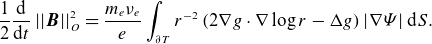(4.19) \begin{equation} \begin{split}{ \frac {1}{2}\frac {\rm d}{{\rm d}t}\left \lvert \left \lvert \boldsymbol{B} \right \rvert \right \rvert ^2_{O}=\frac {m_e\nu _e}{e}\int _{\partial T}r^{-2}\left ({2\nabla g\cdot \nabla \log r-\Delta g}\right ){\left \lvert {\nabla \varPsi }\right \rvert }\,{\rm d}S. }\end{split} \end{equation}

5. Modified neutral point argument

Cowling’s theorem is related to the so-called neutral point argument. Let us see how the neutral point argument changes in the present setting. Suppose that the equilibrium flux function $\varPsi _{\infty }$ is a well-behaved non-constant function in $\mathbb{R}^3$ . Then, by symmetry, it will attain local maximima or minimima somewhere in $\mathbb{R}^3$ . 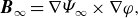At these neutral points, $\nabla\Psi_{\infty}$ and $\boldsymbol{B}_{\infty}=\nabla\Psi_{\infty} \times \nabla\varphi$ vanish. Let N denote a neutral point, and consider a circle C of radius $\epsilon\sim \lvert {\boldsymbol{B}_{\infty }({N+\epsilon \boldsymbol{\delta }})}\rvert$ , where $\boldsymbol{\delta }$ is some unit vector. Let $\Sigma _C$ denote a surface in the $({r,z})$ -plane, with normal $\boldsymbol{n}_C=r\nabla \varphi$ , enclosed by $C$ and such that $N\in \Sigma _C$ . Using Ohm’s law (3.1), Stokes’ theorem and noting that, at equilibrium, the electric field $\boldsymbol{E}_{\infty }=-\nabla \varPhi _{\infty }$ is given as the gradient of a single-valued potential $\varPhi _{\infty }({{r,z}})$ , we have

(5.1) \begin{equation} \begin{split}{ 0=\int _{\Sigma _C}\boldsymbol{E}_{\infty }\cdot \boldsymbol{n}_C\,{\rm d}S= \int _{\Sigma _C}\boldsymbol{B}_{\infty }\times \boldsymbol{u}_{\infty }\cdot \boldsymbol{n}_C \,{\rm d}S+\frac {\eta }{\mu _0}\int _C\boldsymbol{B}_{\infty }\cdot {\rm d}\boldsymbol{l}. }\end{split} \end{equation}

However, by construction, $\Sigma _C=\pi \epsilon ^2$ while $C=2\pi \epsilon$ . In proximity of $N$ , (5.1) can thus be satisfied only if $ ({\mu _0}/{\eta })\boldsymbol{u}_{\infty }\sim {\epsilon ^{-1}}$ , implying that $\boldsymbol{u}_{\infty }$ is singular at $N$ for non-vanishing and bounded coefficients $\eta$ and $\mu _0$ . If the same argument is applied to the modified Ohm’s law (3.7), one obtains

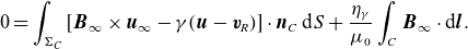(5.2) \begin{equation} \begin{split}{ 0=\int _{\Sigma _C}\left [{\boldsymbol{B}_{\infty }\times \boldsymbol{u}_{\infty }-\gamma ({\boldsymbol{u}-\boldsymbol{v}_{\!R}})}\right ]\cdot \boldsymbol{n}_C \,{\rm d}S+\frac {\eta _{\gamma }}{\mu _0}\int _C\boldsymbol{B}_{\infty }\cdot {\rm d}\boldsymbol{l}. }\end{split} \end{equation}

Now, the second and third terms on the right-hand side are both second-order terms in $\epsilon$ , and the neutral point argument does not apply.

We conclude this section by noting that modifying Ohm’s law only by retaining the Hall effect does not suffice to invalidate the neutral point argument. This is because $ \boldsymbol{J}_{\infty } \times \boldsymbol{B}_{\infty } \cdot \boldsymbol{n}_C = 0$ , given that $ \boldsymbol{J}_{\infty } \times \boldsymbol{n}_C = \boldsymbol{0}$ .

6. Axially symmetric poloidal equilibrium configurations

Let us construct axially symmetric poloidal equilibrium configurations, i.e. steady solutions of the induction equation such that

(6.1a) \begin{align} \boldsymbol{B}_{\infty }&=\nabla \varPsi _{\infty }\times \nabla \varphi ,\\[-10pt]\nonumber \end{align}

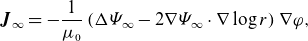(6.1b) \begin{align} \boldsymbol{J}_{\infty }&=-\frac {1}{\mu _0}\left ({\Delta \varPsi _{\infty }-2\nabla \varPsi _{\infty }\cdot \nabla \log r}\right )\nabla \varphi ,\\[-10pt]\nonumber \end{align}

(6.1c) \begin{align} \boldsymbol{E}_{\infty }&=-\nabla \varPhi _{\infty },\\[-10pt]\nonumber \end{align}

(6.1d) \begin{align} \boldsymbol{u}_{\infty }&=\nabla \varTheta _{\infty }\times \nabla \varphi +g_{\infty }\nabla \varphi . \end{align}

Recalling the modified Ohm’s law (3.7), the equilibrium equation is

(6.2) \begin{align} -\nabla \varPhi _{\infty } & =\left (\!{\nabla \varTheta _{\infty }\times \nabla \varphi \cdot \nabla \varPsi _{\infty }-\frac {\eta _{\gamma }}{\mu _0}\Delta \varPsi _{\infty }+2\frac {\eta _\gamma }{\mu _0}\nabla \varPsi _{\infty }\cdot \nabla \log r-\gamma g_{\infty }+\frac {1}{2}\gamma \varOmega r^2}\right )\!\nabla \varphi \nonumber\\& \quad -\frac {g_{\infty }}{r^2}\nabla \varPsi _{\infty }-\gamma \nabla \varTheta _{\infty }\times \nabla \varphi . \end{align}

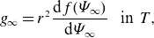
The poloidal component of $\boldsymbol{u}_{\infty }$ can be eliminated by setting $\varTheta _{\infty }=\mathrm{constant}$ . However, the electrostatic potential must be single-valued, leading to $g_{\infty }=r^2 {\rm d}f({\varPsi _{\infty }}){\rm d}\varPsi _{\infty }$ and $\varPhi _{\infty }=f({\varPsi _{\infty }})$ . The equilibium flux function $\varPsi _{\infty }$ is then determined by a Poisson equation. The full set of equilibrium equations is

(6.3a) \begin{align} \Delta \varPsi _{\infty }=2\nabla \varPsi _{\infty }\cdot \nabla \log r-\frac {\gamma \mu _0}{\eta _{\gamma }} r^2\left ({\frac {{\rm d}f({\varPsi _{\infty }})}{{\rm d}\varPsi _{\infty }}-\frac {\varOmega }{2}}\right )\,\,\,\,\mathrm{in}\,\,T, \end{align}

(6.3b) \begin{align} \varPhi _{\infty }=f({\varPsi _{\infty }})\,\,\,\,\mathrm{in}\,\,T,\end{align}

(6.3c) \begin{align} g_{\infty }=r^2\frac {{\rm d}f({\varPsi _{\infty }})}{{\rm d}\varPsi _{\infty }}\,\,\,\,\mathrm{in}\,\,T,\end{align}

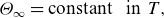(6.3d) \begin{align} \varTheta _{\infty }=\mathrm{constant}\,\,\,\,\mathrm{in}\,\,T, \end{align}

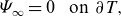(6.3e) \begin{align} \varPsi _{\infty }=0\,\,\,\,\mathrm{on}\,\,\partial T, \end{align}

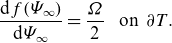(6.3f) \begin{align} \frac {{\rm d}f({\varPsi _{\infty }})}{{\rm d}\varPsi _{\infty }}=\frac {\varOmega }{2}\,\,\,\,\mathrm{on}\,\,\partial T. \end{align}

For given $f({\varPsi _{\infty }})$ , this system admits non-trivial regular solutions in $T$ thanks to the source term proportional to $\gamma$ in the first equation. The result reveals that the electric field $\boldsymbol{E}_{\infty }$ is balanced by the ideal convective term $\boldsymbol{B}_{\infty }\times \boldsymbol{u}_{\infty }$ (see 6.3b ), while the resistive term $\eta _{\gamma }\boldsymbol{J}_{\infty }$ is balanced by the friction term $-\gamma ({\boldsymbol{u}_{\infty }-\boldsymbol{v}_{\!R}})$ as shown in (6.3a ). This type of force balance is consistent with kinetic theory of plasmas, which informs us that equilibria of the Boltzmann equation usually belong to the kernel of the collision operator, i.e. in a steady-state, ideal terms and dissipative terms vanish independently (see e.g. Sato & Morrison (2024) and references therein). Indeed, MHD and related two-fluid theories are reduced models originating from kinetic theory. As previously noted, zero magnetic field solutions are permitted when $g_{\infty } = ({r^2 \varOmega })/{2}$ in $T$ . Additionally, it is important to observe that the toroidal component of the fluid velocity, $g_{\infty } \nabla \varphi$ , can deviate significantly from the planet’s rotation speed, $\boldsymbol{v}_{\!R} = ({1}/{2}) \varOmega r^2 \nabla \varphi$ , within $T$ when a non-zero magnetic field is present (see 6.3a ).

We also remark that $\boldsymbol{J}_{\infty }$ vanishes on $\partial T$ due to the boundary condition (6.3f ) coming from (4.17). Hence, for any $\boldsymbol{x}\in \mathbb{R}^3$ , the (continuous) magnetic field vanishing at infinity and corresponding to the current distribution resulting from system (6.3) can be obtained through the Biot–Savart integral,

(6.4) \begin{equation} \begin{split}{ \boldsymbol{B}_{\infty }({\boldsymbol{x}})=\frac {\mu _0}{4\pi }\int _{T}\frac {\boldsymbol{J}_{\infty }({\boldsymbol{x}'})\times \left ({\boldsymbol{x}-\boldsymbol{x}'}\right )}{\left \lvert {\boldsymbol{x}-\boldsymbol{x}'}\right \rvert ^3}\,{\rm d}V'. }\end{split} \end{equation}

The properties of the Biot–Savart integral (6.4), as well as a generalisation to bounded domains, can be found in Enciso, Garcia-Ferrero & Peralta-Salas (2018). We remark that since the current density $\boldsymbol{J}_{\infty }$ is an axially symmetric toroidal flow, it follows that in $O$ , the equilibrium magnetic field $\boldsymbol{B}_{\infty }$ is an axially symmetric dipole-type magnetic field.

7. Concluding remarks

We have proposed a novel dynamo model that incorporates a modified Ohm’s law within a toroidal volume. The geometry of this toroidal volume, inspired by analogies with fusion plasma physics, can be viewed as a nearly spherical dynamo-active region enclosed by a liquid shell surrounding a planetary core. It is important to note that, whether the system involves liquid iron in rocky planets or ionised hydrogen in gas giants, its electromagnetic behaviour is fundamentally governed by microscopic interactions between ions and electrons, thereby justifying the use of a two-fluid model. In this framework, Ohm’s law is modified to account for the dissipative force associated with electron collisions that tends to align macroscopic flows with the planet’s rotation speed. This force is modelled either as a frictional damping term or as a viscous force. Specifically, the two models examined are as follows. The first model introduces a frictional (damping) force that tends to align the fluid velocity with the planet’s rotation speed. The second model treats the dissipative force as viscous dissipation, under the assumption that the rotating fluid shell adheres to a Navier–Stokes reduction of the underlying kinetic equations. Our analysis shows that this dissipative force can be comparable to the conventional resistive force associated with electron–ion collisions in the standard formulation of Ohm’s law. Therefore, it should not be neglected.

The presented approach indeed enables the formation of axially symmetric steady-state magnetic fields, circumventing traditional spherical geometries and anti-dynamo theorems. The key components of our model include: (i) identifying the dissipative force acting on the fluid shell, in addition to collisional resistive forces, as a critical factor in the electron momentum equation; (ii) modelling the convecting region as a toroidal volume, which allows for non-trivial steady states of the induction equation; (iii) focusing on steady states where ideal and dissipative terms balance independently.

Note that the governing equation, e.g. (4.6), allows for a zero magnetic field solution when the toroidal velocity matches the planet’s rotational speed, indicating that the system is not frictionally driven. This implies that the current model can spontaneously generate a magnetic field purely through fluid motion. These findings adhere to anti-dynamo theorems: we demonstrate how Cowling’s theorem and the neutral point argument are modified by the dissipative force, enabling the existence of non-trivial, axially symmetric equilibrium magnetic fields.

Our model successfully captures the essence of a dynamo, producing a stable dipolar magnetic field and providing valuable insights into the long-term operation and stability of geophysical and astrophysical dynamos. The model’s foundation in partial differential equations ensures broad applicability, including potential generalisations to oscillating magnetic field amplification. To determine the precise range of parameters for which the theory is applicable, experimental and numerical validation are necessary.

We conclude by speculating on a scenario in which the flows considered in this work could be sustained beyond the kinematic dynamo framework. Specifically, one may consider a viscous MHD system governed by a modified Ohm’s law, where the initial kinetic energy of the plasma gradually decreases due to viscous dissipation, while magnetic energy increases through dynamo action. Boundary interactions lead to angular momentum exchange, with frictional effects tending to align the plasma flow with the background rotation. As the system evolves, it may approach a force-balanced configuration, resulting in a reduced kinetic energy state and a self-consistently sustained magnetic field. This scenario highlights the potential for self-consistent dynamo action compatible with the flows described here. An alternative scenario is also plausible, in which, however, the magnetic field is eventually lost. Initially, the magnetic field is amplified while there exists a mismatch between the angular velocity of the ions and that of the domain boundary. Once frictional forces realign the plasma flow with the background rotation, the dynamo action would cease. Subsequently, the magnetic energy would gradually dissipate due to the plasma resistivity. The detailed investigation of such coupled evolution is left for future work.