Tessellation-based analysis of impurity clustering in the edge plasma of tokamaks

Abstract

Confinement quality in fusion plasma is influenced significantly by the presence of heavy impurities, which can lead to radiative heat loss and reduced confinement. This study explores the clustering of heavy impurity, i.e. tungsten in edge plasma, using high-resolution direct numerical simulations of the Hasegawa–Wakatani equations. We use the Stokes number to quantify the inertia of impurity particles. It is found that particle inertia will cause spatial intermittency in particle distribution and the formation of large-scale structures, i.e. the clustering of particles. The degrees of clustering are influenced by the Stokes number. To quantify these observations, we apply a modified Voronoi tessellation, which assigns specific volumes to impurity particles. By determining time changes of these volumes, we can calculate the impurity velocity divergence, which allows the clustering dynamics to be assessed. To quantify the clustering statistically, several approaches are applied, such as probability density function (PDF) of impurity velocity divergence and joint PDF of volume and divergence.

1 Introduction

Fusion reactors aim to achieve fusion reactions by confining and heating a plasma mixture of ions and electrons at extremely high temperatures. Impurities in fusion plasmas can profoundly affect performance and stability. The impurities primarily originate from the interaction between the intense heat of the plasma and the tokamak's walls. Their presence can lead to significant radiation losses and make it challenging to maintain the requisite temperatures for fusion reactions (Wesson & Campbell 2011). These impurities can also dilute the primary fusion fuel, thereby reducing the overall fusion reaction rate. In addition, strong radiation on the plasma's edge can drastically reduce electrical conductivity, leading to disruptions in the current profile inside the $q=2$ surface (Stangeby 2000). Moreover, before reaching density limits, plasmas often develop multifaceted asymmetric radiation from the edge (MARFE) which produces localised radiation, usually at the inner wall or the X-point, caused by strong impurity radiation near the edge (Stangeby 2000).

The behaviour of plasma flow within reactors, specifically in the edge region of a tokamak, is influenced by drift-wave turbulence and zonal flows. Our high-resolution simulations to understand this flow are based on the Hasegawa–Wakatani (HW) model (Hasegawa & Wakatani 1983), which provides insights into cross-field transport caused by electrostatic drift waves. The electric field perpendicular to magnetic field lines is particularly significant because it strongly drives cross-field fluxes, and influences edge pressure profiles and overall stability (Zhang, Guo & Diamond 2020). The HW equations are particularly useful for studying plasma turbulence, which is a major cause of energy loss in tokamak devices. These equations capture the essential physics of drift-wave turbulence. Despite their simplicity, the HW equations have proven to be a powerful tool for understanding the complex dynamics of plasma behaviour in tokamak devices (Horton 2012).

For the particles, the Lagrangian perspective has been of interest in recent years (Bos et al. 2010; Kadoch, Bos & Schneider 2010; Kadoch et al. 2022; Gheorghiu, Militello & Rasmussen 2024). This perspective delves into transport properties by analysing the trajectories of multiple tracer particles. Through numerical simulations, we solve equations about these particle trajectories within particular plasma flow velocity fields, such as the $\boldsymbol {E} \times \boldsymbol {B}$ field. This method highlights the significant effect of coherent structures on transport. The interplay between eddy trapping and zonal shear flows results in non-diffusive transport (del Castillo-Negrete, Carreras & Lynch 2004; van Milligen, Sanchez & Carreras 2004; Krasheninnikov, D'Ippolito & Myra 2008; Krasheninnikov 2024; Krasheninnikov & Smirnov 2024). Both experimental and numerical findings confirm the presence of these coherent structures in edge turbulence (Krasheninnikov et al. 2008).

In fusion plasma research, existing studies have focused on passive flow tracers in edge plasma, using the HW model, without taking inertial effects into account (Futatani et al. 2008a,b; Futatani, Benkadda & del Castillo-Negrete 2009). In the work by Priego et al. (2005), the inertial effect is considered and a fluid model for impurities is used, wherein the impurity particle velocity is considered to be the sum of the $\boldsymbol {E} \times \boldsymbol {B}$ and polarisation drifts. The polarisation drift, accounting for impurity particle inertia, is a higher-order correction to the $\boldsymbol {E} \times \boldsymbol {B}$ drift velocity and introduces compressible effects. In contrast to a fluid model, we track each impurity particle individually. In addition, we assume that heavy impurity particles may ‘lag behind’ plasma flow velocity due to the significant inertia. Indeed, the role of inertia in particle advection by turbulent flows is well-documented in fluid dynamics and is known to result in clustering around vortical structures (Provenzale 1999). Our study aims to analyse possible clustering effects for impurities in magnetised plasma.

A key element in understanding these heavy impurities is their tendency for self-organisation. This self-organisation is seen in clusters of impurities and void regions (Monchaux, Bourgoin & Cartellier 2010; Lin et al. 2024). It can be mathematically quantified by deviation from Poissonian statistics (Oujia, Matsuda & Schneider 2020; Maurel-Oujia, Matsuda & Schneider 2023). The goal is to investigate the statistical signature of clustering and void regions. Recent results for hydrodynamics turbulence are promising (Matsuda, Schneider & Yoshimatsu 2021). Finite-time measures to quantify divergence and the rotation of the particle velocity by determining the volume change rate of the Voronoi cells and their rotation, respectively, were proposed by Oujia et al. (2020) and Maurel-Oujia et al. (2023) and applied in the context of hydrodynamic turbulence. Here we apply them to characterise the dynamics of the self-organisation of heavy impurities in plasma and assess their clustering and void formation.

The paper is structured as follows. In § 2 we outline the theoretical basis used for simulation, tessellation-based analysis method and numerical set-up. Section 3 details our numerical simulation results and tessellation-based analysis results. Finally, § 4 summarises our findings and suggests potential directions for future investigations.

2 Models for simulation and analysis method

2.1 HW model

The model for our numerical simulations is based on the HW equations for plasma edge turbulence driven by drift-wave instability (Hasegawa & Wakatani 1983). Our focus in this study is on the two-dimensional slab geometry of the HW model; see, e.g., Kadoch et al. (2022). The two-dimensional HW model is a representative paradigm for understanding the nonlinear dynamics of drift-wave turbulence. Figure 1 depicts a representation of the flow configuration.

Figure 1. Two-dimensional slab geometry. In the tokamak edge, the two-dimensional slab geometry flow configuration is depicted using the HW system. Here, the radial direction is represented by $x$, whereas $y$ is the poloidal direction. There is an imposed mean plasma density gradient $\boldsymbol {\nabla }{n_0}$ in the radial direction. The two-dimensional flow is computed within a square domain measuring 64 Larmor radii ($\rho _s$) on each side, as indicated by the green outline. On the right, a vorticity field is displayed.

The magnetic field lines are assumed to be straight and perpendicular to the slab. Ions are considered cold, ignoring temperature gradient effects. The key variables are normalised as detailed in the work done by Bos et al. (2010) and Futatani et al. (2011),

(2.1a)\begin{equation} x/\rho_{{s}} \rightarrow x,\quad \omega_{\mathrm{ci}} t \rightarrow t, \quad e \phi / T_{\rm e} \rightarrow \phi,\quad n_{1} / n_{0} \rightarrow n, \end{equation}

where $\rho _s$ is the ion Larmor radius at electron temperature $T_{\rm e}$. It is defined as ${\rho _s = {\sqrt {T_{\rm e}/m_{\rm i}}}/{\omega _{\rm ci}}}$, where $\omega _{\rm ci}$ is the ion cyclotron frequency. Here $n_{1}$ and $n_{0}$ represent plasma density fluctuation and equilibrium density, whereas $\phi$ indicates electrostatic potential fluctuation. The HW model consists of two equations that describe the evolution of plasma potential and fluctuating plasma density, respectively:

(2.2)\begin{gather} \left(\frac{\partial}{\partial t}- \mu_{\nu} \nabla^{2}\right) \nabla^{2} \phi=[\nabla^{2} \phi, \phi]+c(\phi-n), \end{gather}

(2.3)\begin{gather}\left(\frac{\partial}{\partial t}-\mu_{\rm D} \nabla^{2}\right) n=[n, \phi]-\kappa \frac{\partial \phi}{\partial y}+c(\phi-n), \end{gather}

where $\mu _{\rm D}$ is cross-field diffusion coefficient and $\mu _{\nu }$ is kinematic viscosity. The term $\kappa$, defined as $\kappa \equiv - \partial _{x} \ln (n_{0})$, is a measure of the plasma density gradient. Here $\kappa$ is assumed constant, implying $n_{0} \propto \exp (-\kappa x)$. The Poisson bracket is defined as $[A, B]=({\partial A}/{\partial x}) ({\partial B}/{\partial y})-({\partial A}/{\partial y})({\partial B}/{\partial x})$. In these equations, the electrostatic potential $\phi$ is the stream function for the $\boldsymbol {E} \times \boldsymbol {B}$ velocity, represented by $\boldsymbol {u}=\nabla ^{\perp } \phi$, where $\nabla ^{\perp }=(-{\partial }/{\partial y}, {\partial }/{\partial x})$. Thus, $u_x=-{\partial \phi }/{\partial y}$ and $u_y={\partial \phi }/{\partial x}$ with vorticity $\omega =\nabla ^2 \phi$.

In the equations, $c$ is the so-called adiabaticity parameter which measures the parallel electron response. It is defined as

(2.4)\begin{equation} c=\frac{T_{\rm e} k_{{\parallel}}^{2}}{\mathrm{e}^{2} n_{0} \eta \omega_{\rm ci}}. \end{equation}

With $\eta$ as electron resistivity and $k_{\parallel }$ as the effective parallel wavenumber, parameter $c$ determines the phase difference between electrostatic potential and plasma density fluctuations. The model described above is the classical Hasegawa–Wakatani (cHW) model. For $c\gg 1$ (adiabatic limit), the model reduces to the Hasegawa–Mima equation, where electrons follow a Boltzmann distribution. At $c \ll 1$ (hydrodynamic limit), the system reduces to a form that is analogous to the two-dimensional Navier–Stokes equation, where density fluctuations are passively influenced by the $\boldsymbol {E} \times \boldsymbol {B}$ drift. Notably, for $c \sim 1$ (quasi-adiabatic regime), a phase shift between the potentials and densities is observed, enabling particle transport and reflecting a complex interplay between them. To obtain zonal flow, a revised version of the model, known as the modified Hasegawa–Wakatani (mHW) model, can be considered. This modification was introduced in Pushkarev, Bos & Nazarenko (2013) which consists in setting the coupling term $c(\phi -n)$ to zero for modes $k_y= 0$. In this paper, we focus on the quasi-adiabatic regime, i.e. $c = 0.7$ (cHW model), which is relevant to the edge plasma of tokamaks (Bos et al. 2010). For readers interested in the results of other regimes, we refer to Appendix A.

2.2 Impurity particles model

Earlier research (Futatani et al. 2008a,b, 2009) assumed that impurity particles, due to no inertia, act as ‘passive tracers’ aligning closely with fluid flow. Yet, for heavier particles, this assumption might not always hold, particularly when the particles have significant mass, leading to notable inertial effects. To address this, the Stokes number ($St$) can be introduced (see, e.g., Oujia et al. 2020), a dimensionless parameter that quantifies particle inertia in fluid flow. The Stokes number is defined as

(2.5)\begin{equation} St = \frac{\tau_{\rm p}}{\tau_{\eta}}, \end{equation}

where $\tau _{\rm p}$ denotes the impurity particle's relaxation time, it measures the time the particle takes to adapt to fluid flow alterations. A smaller $\tau _{\rm p}$ means the particle adapts faster. On the other hand, $\tau _{\eta }$ is the characteristic timescale for turbulence, indicating how fast the fluid flow changes. A smaller $\tau _{\eta }$ suggests more rapid turbulence changes. A high Stokes number means that a particle's movement is primarily driven by inertia, causing it to keep its direction despite fluid changes. In previous studies (Futatani et al. 2008a,b, 2009), the impurity particles are treated as passive tracers of the flow, indicating $\tau _{\rm p} = 0$. However, here we consider heavy impurity particles with $\tau _{\rm p} > 0$, for instance tungsten.

The heavy impurity particles are modelled as charged point particles. They are considered as test particles, which means that there is no impurity–impurity interaction and impurities have no effect on the plasma dynamics, whereas the plasma flow velocity affects the motion of impurities (one-way coupling). Impurities in our model are assumed to be cold, just as with the treatment of ions in bulk plasma. Thus, thermal motion of impurities could be neglected for simplicity. The impurity particles experience not only the Lorentz force due to the electric and magnetic fields, but also drag force resulting from momentum transfer with plasma ions. Positive plasma ions transfer momentum to heavy charged impurity particles by interacting with electrostatic potential in the vicinity of the impurity particle. The transfer of momentum from electrons to impurities is negligible due to their small mass. Coulomb scattering theory provides, macroscopically, an approximation of a drag force $F_{\rm drag}$ dependent on the relative velocity between the macroscopic velocity of the plasma ion and the velocity of the impurity particle (Kilgore et al. 1993): $F_{\rm drag} = K_{\mathrm {mt}} n_{\rm i} m_{\rm i} v_{\rm r}$, where $v_{\rm r}$ is the relative velocity between the macroscopic velocity of the plasma ions and the impurity particles, $K_{\mathrm {mt}}$ is the momentum transfer coefficient, $n_{\rm i}$ is the plasma ion density and $m_{\rm i}$ is the ion mass of the plasma. This drag force tends to reduce the velocity difference, causing the impurity particles to relax to the plasma flow velocity. The relaxation time of the impurity particle $\tau _{\rm p}$ is the period during which impurity particles adjust to the plasma flow due to the drag force. In our model, we approximate this drag force as $m_{\rm p}(u_{\rm p}-v_{\rm p})/\tau _{\rm p}$, which is proportional to the relative velocity between the plasma flow and impurities. The relaxation time can be expressed as $\tau _{\rm p}={m_{\rm p}}/{K_{\mathrm {mt}} n_{\rm i} m_{\rm i}}$. This relation highlights that $\tau _{\rm p}$ is inversely proportional to the plasma ion density and momentum transfer coefficient, while directly proportional to the impurity mass. Given this relationship, as the ion density $n_{\rm i}$ increases, the relaxation time decreases, leading to faster coupling of the impurity particles to the plasma flow. Conversely, larger impurity masses result in longer relaxation times, reflecting the slower response of heavier particles to the plasma flow. According to Newton's second law:

(2.6)\begin{gather} m_{\rm p} \frac{{\rm d} \boldsymbol{v}_{{\rm p},j}}{{\rm d} t} = \frac{m_{\rm p}(\boldsymbol{u}_{{\rm p},j}- \boldsymbol{v}_{{\rm p},j}) }{\tau_{\rm p}} + Ze(\boldsymbol{E}(\boldsymbol{x}_{{\rm p},j}) + \boldsymbol{v}_{{\rm p},j} \times \boldsymbol{B}), \end{gather}

(2.7)\begin{gather}\boldsymbol{E}(\boldsymbol{x}_{{\rm p},j})={-}\boldsymbol{\nabla} \phi(\boldsymbol{x}_{{\rm p},j}). \end{gather}

Equation (2.6) describes the forces exerted on each heavy impurity particle, denoted by $j$ ($\,j=1, \ldots, N_{\rm p}$, with $N_{\rm p}$ being the total number of particles). Here $Z$ is charge state of the impurity particle and $e$ is the elementary charge. The variable $\boldsymbol {v}_{{\rm p},j}$ is the $j$th particle's velocity, whereas $\boldsymbol {u}_{{\rm p},j}$, $\boldsymbol {E}(\boldsymbol {x}_{{\rm p},j})$ and $\boldsymbol {\nabla } \phi (\boldsymbol {x}_{{\rm p},j})$ represent the fluid velocity, electric field and gradient of potential at the particle's location $\boldsymbol {x}_{{\rm p},j}$, respectively. Let us note that when ${\tau _{\rm p} = 0}$, we recover the situation studied in previous works (Futatani et al. 2008a,b, 2009). In this case, the impurity particles are considered as passive tracers of the flow, i.e. $\boldsymbol {v}_{{\rm p},j} \equiv \boldsymbol {u}_{{\rm p},j}$. Applying the same normalisation as used for the HW equation, we obtain

(2.8)\begin{equation} \frac{{\rm d} \boldsymbol{v}_{{\rm p},j}}{{\rm d} t}=\frac{(\boldsymbol{u}_{{\rm p},j}-\boldsymbol{v}_{{\rm p},j})}{\tau_{\rm p}}+ \alpha (-\boldsymbol{\nabla} \phi(\boldsymbol{x}_{{\rm p},j})+\boldsymbol{v}_{{\rm p},j} \times \boldsymbol{b}),\end{equation}

where $\alpha ={Zm_{\rm i}}/{m_{\rm p}}$, $m_{\rm i}$ is the ion mass of the plasma and $\boldsymbol {b}$ represents the unit vector along the direction of the magnetic field. Combining with the equation:

(2.9)\begin{equation} \frac{{\rm d}\kern0.07em\boldsymbol{x}_{{\rm p},j}}{{\rm d} t} = \boldsymbol{v}_{{\rm p},j},\end{equation}

it is thus possible to compute the trajectory of the impurity particles.

2.3 Modified Voronoi tessellation

Impurity particles satisfy the conservation equation:

(2.10)\begin{equation} D_t n_{\rm p}={-}n_{\rm p} \boldsymbol{\nabla} \boldsymbol{{\cdot}} {\boldsymbol{v}_p},\end{equation}

where $D_t$ is the Lagrangian derivative, $n_{\rm p}$ is the impurity particle number density and $\boldsymbol {v}_{\rm p}$ the particle velocity. From this equation, the divergence of particle velocity $\boldsymbol {\nabla } \boldsymbol {{\cdot }} {\boldsymbol {v}_{\rm p}} = -{D_t n}/{n}$ is crucial to understand. A positive divergence ($\boldsymbol {\nabla } \boldsymbol {{\cdot }} {\boldsymbol {v}_{\rm p}} > 0$) leads to density decrease, whereas a negative divergence, i.e. convergence ($\boldsymbol {\nabla } \boldsymbol {{\cdot }} {\boldsymbol {v}_{\rm p}} < 0$), causes an increase in density. To quantify the divergence, we employ the modified version of the classical Voronoi tessellation technique, which uses the centre of gravity, instead of the circumcentre of the Delaunay cell, to define Voronoi cell vertices. The purpose of this method is to assign a volume to each impurity particle, enabling the subsequent calculation of the divergence. More details about the classical and modified Voronoi tessellation and their difference can be found in Oujia et al. (2020) and Maurel-Oujia et al. (2023). The modified Voronoi tessellation divides a plane into regions according to the positions of impurity particles, which allows us to assign a cell, called a ‘modified Voronoi cell’, and thus a corresponding volume $V$ to each particle. Each cell can be considered as the region of influence of an impurity particle. In our two-dimensional scenario, the volume of the cell is determined by calculating its area. Figure 2 shows the modified Voronoi tessellation. In the figure, clustered particles are represented by small cells and void regions are represented by large cells.

Figure 2. (a) Electric potential $\phi$ (stream function) and $10^4$ superimposed impurity particles for $St = 1$ in the case $c = 0.7$ (cHW model). (b) A magnified view with modified Voronoi tessellation. Large cells correspond to void regions, small cells represent clusters.

To compute the divergence of impurity particle velocity ${\mathcal {D}}$ we analyse particle distributions at two time instants $t^k$ and $t^{k+1}=t^k+\Delta t$, where $\Delta t$ is the time step of the simulation and $k$ is the discrete time index. Each particle distribution snapshot is assessed using modified Voronoi tessellation. The inverse of volume, $1/V$, approximates the local particle number density $n_{\rm p}$ in the discrete setting. It is proved that (Oujia et al. 2020; Maurel-Oujia et al. 2023)

(2.11)\begin{equation} {\mathcal{D}} ({\boldsymbol{v}_{\rm p}}) ={-}\frac{1}{n_{\rm p}} D_t n_{\rm p} = \frac{2}{\Delta t} \frac{V^{k+1}-V^k}{V^{k+1}+V^k} + O\left(\frac{1}{N_{\rm p}}, \Delta t\right).\end{equation}

Thus, by measuring the volume change of each particle between $t^k$ and $t^{k+1}$, we can determine the discreet divergence of its velocity ${\mathcal {D}}({\boldsymbol {v}_{\rm p}}$). The velocity divergence of impurity particles measures the rate of volume change for a particle group over time, indicating how much the particle velocity field is spreading out or converging at a particular point in space.

2.4 Numerical set-up

The simulation was conducted within a domain that spans an area $A$ of $64 \times 64$ with periodic boundary condition. The domain was discretised to a resolution $R$ of $1024 \times 1024$ grid points. The time step $\Delta t$ was $5\times 10^{-4}$. The number of impurity particles $N_{\rm p}$ was $10^6$. The adiabaticity parameter $c$ is $0.7$. The values of specific physical parameters are listed in table 1. The characteristic time scale of turbulence, $\tau _{\eta }$, is defined as $1 / \sqrt {2 Z_{\rm ms}}$, with $Z_{\rm ms}$ denoting one half of the mean-square vorticity. In the simulation, $\tau _{\eta } = 0.35$ in the statistically steady flow. The simulations are based on the work of Kadoch et al. (2022) where the flow is initialised with Gaussian random fields. Here we start the simulations with a flow already being in the statistically steady state (i.e. after the long transition phase of drift-wave instabilities; see Kadoch et al. 2022) and one million uniformly distributed heavy impurity particles with random velocity are injected.

Table 1. Simulation parameters for the flow: $A$, domain area; $R$, grid resolution; $\Delta t$, time step; $N_{\rm p}$, number of impurity particles; $\mu _{\rm D}$, diffusion coefficient; $\mu _{\nu }$, kinematic viscosity; $\kappa \equiv - \partial _{x} \ln (n_{0})$, a measure of the plasma density gradient; $c$, adiabaticity parameter.

For the impurity particles, we focus on tungsten $_{74}^{184}\mathrm {W}^{20+}$, a heavy metal that can be made from the material that is exposed to the high heat flux in ASDEX-Upgrade (Krieger, Maier & Neu 1999) and EAST (Yao et al. 2016), expecting the same situation for ITER (Pitts et al. 2009). For $_{74}^{184}\mathrm {W}^{20+}$, $\alpha = Zm_{\rm i}/m_{\rm p} = 0.22$. As for Stokes number $St = \tau _{\rm p}/\tau _\eta$, $\tau _\eta = 0.35$ in the statistically steady state of flow for $c = 0.7$ (cHW model), but the exact value of $\tau _{\rm p}$ for $_{74}^{184}\mathrm {W}^{20+}$ is unknown. To resolve this, we explore a range of $\tau _{\rm p}$ values spanning several orders of magnitude, resulting in Stokes numbers $St = 0$, 0.05, 0.5, 1, 5, 10 and $50$. This parametric approach allows us to systematically explore the dynamics of tungsten impurity, from particles that are tightly coupled to the flow ($St \ll 1$) to those that are essentially independent of the flow ($St \gg 1$). The simulation parameters are listed in table 2.

Table 2. Stokes numbers used in the simulation.

The system of HW equations, specifically (2.2) and (2.3) are solved using a classical pseudospectral method (Canuto et al. 2007). The equations governing the motion of the impurity particles, namely (2.8) and (2.9), are solved using a second-order Runge–Kutta (RK2) scheme and linear interpolation is used for computing the fluid velocity at the particle position. The code of this study builds upon that used in the research done by Kadoch et al. (2022).

3 Results

3.1 Simulation results

The analysed data set consists of the electric potential $\phi$ (stream function), particle position and velocity data generated by direct numerical simulation (DNS). The contour curves of constant $\phi$ represent the streamlines of the flow field and provide a clear visualisation of fluid flow in two dimensions. Closed contour curves indicate the presence of vortices. Figure 3 illustrates the $\phi$ fields and the behaviour of impurity particles in statistically steady state within the quasi-adiabatic regime ($c = 0.7$, cHW model), where impurity particles are considered as passive tracers without considering inertial effect ($St = 0$). As shown by figure 3 impurity particles are distributed randomly. Figure 4 shows that with increasing Stokes numbers ($St = 0.05, 0.5, 1$), particle inertia begins to dominate, causing them to deviate from the fluid streamlines due to Coriolis force induced by the vortices. This deviation causes them to concentrate where the vorticity is minimal, typically at vortex peripheries. For even higher Stokes numbers ($St = 5, 10, 50$), the impurity particles tend to maintain their trajectories, moving more ballistically and exhibiting reduced clustering. From (2.8), when the coefficient of the flow effect term, $1/\tau _{\rm p} = 1/( \tau _\eta St)$, is much larger than the coefficient term of the Lorentz force $\alpha$, the particle dynamics are primarily governed by the flow, whereas the Lorentz force plays a relatively minor role. For $St = 0.05$, 0.5 and $1$, $1/\tau _{\rm p} = 1/(0.35 St ) \gg \alpha = 0.22$, the particles are more strongly influenced by the fluid flow than by the electromagnetic forces. However, as the Stokes number increases to values such as $St = 10$ and $50$, the particles are less coupled to the fluid flow and the electromagnetic forces start to play an important role. As shown in figure 4, for case $St = 10$ and $50$, the positively charged impurity particles are mostly located in negative potential regions (red region), as expected. The effects of different $\alpha$ values are further explored in Appendix B.

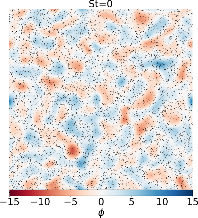
Figure 3. Electric potential field $\phi$ (stream function) superimposing $10^4$ impurity particles (out of $10^6$) for $St = 0$ in statistically steady state within the quasi-adiabatic regime ($c = 0.7$, cHW model).

Figure 4. Electric potential fields $\phi$ (stream function) superimposing $10^4$ impurity particles (out of $10^6$) for various Stokes numbers in statistically steady state within the quasi-adiabatic regime ($c = 0.7$, cHW model).

Let us note that in regions of impurity clustering, where the impurity density may locally increase, there is a risk that clustering could lead to deviations from the assumption of quasi-neutrality that is underlying the derivations of the HW model (Naulin et al. 2006). This strict condition, which requires that the impurity density remains smaller than the bulk current divergence on the characteristic drift-wave time scale, cannot always be guaranteed in regions of intense clustering. Nevertheless, as noted in Naulin et al. (2006), considering impurities as test particles is still valuable for understanding tendencies in impurity transport within a given flow field, and the clustering effects observed in our simulations provide insights into impurity dynamics. We further acknowledge that resolving this discrepancy would require a more sophisticated model that accounts for the back-reaction of impurity densities on the plasma fields and their contribution to quasi-neutrality. Such a model would need to self-consistently address the plasma profile problem in the presence of impurities, which is beyond the scope of the present work, but remains a valuable direction for future research.

3.2 Tessellation-based analysis results

We calculate the volume $V$ for each impurity particle, and then plot the probability density function (PDF) of $V/\bar {V}$, where $\bar {V}$ is the average volume, calculated as $\bar {V} = 64^2/N_{\rm p}$ ($64^2$ is the domain area, $N_{\rm p}$ is the total number of particles). Figure 5(a) shows the PDF of $V/\bar {V}$.

Figure 5. (a) PDF of volume normalised by the mean for different Stokes numbers against the gamma distribution. (b) PDF of the divergence of impurity particle velocity for different Stokes numbers for $_{74}^{184}\mathrm {W}^{20+}(\alpha = 0.22)$ in quasi-adiabatic regime ($c = 0.7$, cHW model).

A random variable $X$ that is gamma-distributed with shape $k$ and scale parameter $\theta$ is denoted $X \sim \varGamma (k, \theta )$. The corresponding PDF is $f(x)=\varGamma (k)^{-1} \theta ^{-k} x^{k-1} \exp (-x / \theta )$. For particles that are distributed randomly, the PDF of the volumes follows a gamma distribution (Ferenc & Néda 2007). For $St = 0$, using the maximum-likelihood PDF estimation for fitting, we find that the PDF of the volumes aligns well with the gamma distribution, specifically we have $\varGamma (1.72, 0.58)$. This suggests, as expected, that the impurity particles are distributed randomly when $St = 0$, indicating no clustering of particles. Let us note that the PDF of the volumes for $St = 0$ obtained using classical Voronoi tessellation follows a gamma distribution $\varGamma (7/2, 2/7)$ (Ferenc & Néda 2007). Since we use a different method, the modified Voronoi tessellation, the fitting gives different values, i.e. $\varGamma (1.72, 0.58)$. The PDF of the volume is typically used to classify ‘cluster cells’ and ‘void cells’ (Monchaux et al. 2010). A cell below a certain threshold is considered a cluster cell, whereas a cell above this threshold is categorised as a void cell. In our study, the threshold is $V/\bar {V} \sim 0.5$. As shown by figure 5(a), when $St$ increases, we observe an increase in the number of cluster cells (with $V/\bar {V} < 0.5$). However, once $St$ exceeds $St = 1$, the number of cluster cells begins to decrease. This is also highlighted by figure 4 which shows that the particles are densely packed for $St =1$.

The PDF of the divergence of impurity particle velocity is displayed in figure 5(b). As shown in figure 5(b), the divergence of the fluid velocity (represented by the divergence of the impurity particle velocity with $St = 0$) is small but not zero. However, as we know, in an incompressible continuous fluid, the divergence of the fluid velocity should be zero. The reason for this discrepancy lies in our computational method, which segments the fluid into separate pieces known as ‘modified Voronoi cells’ as mentioned before. The deformation of a modified Voronoi cell does not correspond to the deformation of a fluid volume in a continuous context. The figure implies that the divergence is attributable to discretisation errors. A negative divergence in a particle velocity field indicates that particles converge towards a point, thus increasing density locally. Conversely, positive divergence shows that particles spread out from a point, reducing the local density. As shown in figure 5(b), for increasing Stokes number, the PDF of divergence ${\mathcal {D}}$ widens, reflecting stronger particles convergence and divergence activities. The symmetry observed in figure 5(b) suggests that positive and negative divergence values are comparable. This balance is due to the conservation of impurity particles.

The joint PDFs of the divergence $\mathcal {D}$ and normalised volume $V/{V}$ show more insight into cluster formation (cf. Figure 6). There is a high probability along $\mathcal {D} = 0$, indicating groups of particles move as an incompressible flow. High negative/positive divergence probability in cluster cells ($V/{V}<0.5$) may be due to the fact that the probability of finding particles in clusters is higher than in void region as illustrated by figure 5(a). As the Stokes number increases, particles deviate more from the fluid flow, increasing their relative velocity. Therefore, high negative/positive divergence could also be from ‘caustics’ where the multi-valued particle velocities at a given position cause large velocity differences between neighbouring particles, leading to extreme divergence (Wilkinson & Mehlig 2005). Figure 7 visually supports this by colouring particles based on their divergence $\mathcal {D}$. From figure 7, we observe that particles with large negative/positive divergence values are densely packed in clusters, indicating simultaneous particles convergence and divergence.

Figure 6. Joint PDF of the volume in log scale and divergence in linear scale for (a) $St = 0.05$, (b) $St = 0.5$, (c) $St = 1$, (d) $St = 5$, (e) $St = 10$ and ( f) $St = 50$ in the quasi-adiabatic regime ($c = 0.7$, cHW model).

Figure 7. Spatial distribution of one million particles coloured with the divergence $\mathcal {D}$ for (a) $St = 0.05$, (b) $St = 0.5$, (c) $St = 1$, (d) $St = 5$, (e) $St = 10$ and ( f) $St = 50$ in the quasi-adiabatic regime ($c = 0.7$, cHW model).

4 Conclusions

In this work, we have studied the spatial distribution of impurity particles in the edge plasma of tokamaks. High-resolution simulations of the plasma flow were based on the paradigmatic model in edge plasma of tokamaks, namely the HW model, whereas the impurity particles were tracked using a Lagrangian method. Assuming that impurity particles have a non-zero relaxation time ($\tau _{\rm p} \neq 0$), which means that the particles do not immediately adapt to fluctuations in plasma flow, we observed the phenomenon of impurity clustering within the plasma. To gain deeper insights into the self-organisation of impurity particles, we employed a modified Voronoi tessellation technique to compute the divergence of impurity particle velocity $\mathcal {D}$. The main results are as follows.

1. (i) The effect of $St$

   • • As $St$ increases, impurities cluster in low-vorticity regions due to their inability to adapt to rapid changes in plasma flow. At high $St$, impurities move randomly with less clustering.

   • • With an increase in $St$, there is a higher probability of observing higher values of negative or positive divergence (for $\alpha = 0.22$). This implies that the impurity particle velocity field is converging or diverging faster. These large values of negative or positive divergence are more likely to be found in cluster cells where $(V/{V} < 0.5$).

2. (ii) The effect of $\alpha$

   • • The influence of $\alpha$ becomes significant only when $St$ is large, which tends to drive the impurity particles into negative electric potential regions.

For future work, it could be interesting to extend the analysis to multi-resolution techniques that would provide a better understanding of the clustering behaviour of impurity particles at different scales; see, e.g., Matsuda et al. (2022). This approach could reveal more details about the spatial distribution and dynamics of clusters that are not apparent at a single scale of observation. Another interesting direction is to explore the transport dynamics of heavy impurity particles for different Stokes number by tracking them for a long time. Finally, the limitation of this work is that we assumed that impurities do not affect plasma flow. Although this simplification allowed for a focused study on impurity particle dynamics, it may not capture the full complexity of the interaction between impurities and plasma flow. A possible extension in future studies is to explore the effect of impurity particles on the plasma flow based on the work of Benkadda et al. (1996).