


1. Introduction
Magnetic reconnection is a fundamental plasma process in the contexts of astrophysical, space and fusion plasmas (Zweibel & Yamada Reference Zweibel and Yamada2009). This process occurs when oppositely directed magnetic field lines interact in the regions of high current density to break and reconnect, altering the magnetic topology and allowing for the rapid conversion of magnetic energy into kinetic and thermal energy. Magnetic reconnection can drive explosive phenomena such as solar flares, coronal mass ejections and geomagnetic storms in the Earth’s magnetosphere (Shibata & Magara Reference Shibata and Magara2011; Burch & Phan Reference Burch and Phan2016; Ruan, Xia & Keppens Reference Ruan, Xia and Keppens2020). It has played a pivotal role in regulating the dynamics of high-energy astrophysical environments, from the solar corona and interstellar medium to distant pulsar magnetospheres and black hole accretion disks (Cerutti, Philippov & Spitkovsky Reference Cerutti, Philippov and Spitkovsky2016; Ripperda, Bacchini & Philippov Reference Ripperda, Bacchini and Philippov2020; Fielding, Ripperda & Philippov Reference Fielding, Ripperda and Philippov2023; Zhang, Pree & Bellan Reference Zhang, Pree and Bellan2023). In particular, reconnection is invoked to understand the particle acceleration and non-thermal emission in many systems (Cerutti, Uzdensky & Begelman Reference Cerutti, Uzdensky and Begelman2012; Sironi & Spitkovsky Reference Sironi and Spitkovsky2014; Guo et al. Reference Guo, Liu, Daughton and Li2015; Brunetti & Lazarian Reference Brunetti and Lazarian2016; Werner et al. Reference Werner, Uzdensky, Cerutti, Nalewajko and Begelman2016; Ghosh & Bhat, Reference Ghosh and Bhat2025). Uncovering the mechanisms of reconnection is essential for explaining these high-energy events and for improving our understanding of plasma behavior across the universe.
Reconnection has been largely studied in two dimensions. It is thought to manifest in different ways: (i) spontaneously as the tearing mode instability, (ii) in steady state known as the Sweet–Parker (SP) model and (iii) as turbulent reconnection. Tearing instability was first studied in the context of magnetic confinement in laboratory plasmas (Furth, Killeen & Rosenbluth Reference Furth, Killeen and Rosenbluth1963; Coppi et al. Reference Coppi, Galvao, Pellat, Rosenbluth and Rutherford1976). Since both tearing modes and the SP model lead to dimensionless reconnection rates that depend on a negative power of the Lundquist number ( $S$
), they could not explain observed time scales pertaining to solar flares. However, more recently, the discovery of the plasmoid instability has been considered to have solved the time scale problem (Loureiro, Schekochihin & Cowley Reference Loureiro, Schekochihin and Cowley2007; Bhattacharjee et al. Reference Bhattacharjee, Huang, Yang and Rogers2009; Cassak, Shay & Drake Reference Cassak, Shay and Drake2009; Uzdensky, Loureiro & Schekochihin Reference Uzdensky, Loureiro and Schekochihin2010; Pucci & Velli Reference Pucci and Velli2013; Comisso et al. Reference Comisso, Lingam, Huang and Bhattacharjee2016). The plasmoid instability is fundamentally a re-emergence of the tearing instability in high-
$S$
), they could not explain observed time scales pertaining to solar flares. However, more recently, the discovery of the plasmoid instability has been considered to have solved the time scale problem (Loureiro, Schekochihin & Cowley Reference Loureiro, Schekochihin and Cowley2007; Bhattacharjee et al. Reference Bhattacharjee, Huang, Yang and Rogers2009; Cassak, Shay & Drake Reference Cassak, Shay and Drake2009; Uzdensky, Loureiro & Schekochihin Reference Uzdensky, Loureiro and Schekochihin2010; Pucci & Velli Reference Pucci and Velli2013; Comisso et al. Reference Comisso, Lingam, Huang and Bhattacharjee2016). The plasmoid instability is fundamentally a re-emergence of the tearing instability in high- $S$
regimes and arises asymptotically beyond
$S$
regimes and arises asymptotically beyond $S\sim 10^4$
, leading to bursty reconnection and the formation of small secondary magnetic islands called plasmoids (Samtaney et al. Reference Samtaney, Loureiro, Uzdensky, Schekochihin and Cowley2009; Landi et al. Reference Landi, Zanna, Papini, Pucci and Velli2015). Importantly, in its nonlinear regime, the plasmoid instability yields reconnection rates that are effectively independent of
$S\sim 10^4$
, leading to bursty reconnection and the formation of small secondary magnetic islands called plasmoids (Samtaney et al. Reference Samtaney, Loureiro, Uzdensky, Schekochihin and Cowley2009; Landi et al. Reference Landi, Zanna, Papini, Pucci and Velli2015). Importantly, in its nonlinear regime, the plasmoid instability yields reconnection rates that are effectively independent of $S$
(Bhattacharjee et al. Reference Bhattacharjee, Huang, Yang and Rogers2009).
$S$
(Bhattacharjee et al. Reference Bhattacharjee, Huang, Yang and Rogers2009).
Complementary to this, the ideal tearing scenario proposed by Pucci & Velli (Reference Pucci and Velli2013) predicts that thin current sheets can become unstable on ideal (Alfvénic) time scales when their aspect ratio scales as $S^{-1/3}$
, leading to reconnection rates that are independent of resistivity. This prediction has been confirmed and extended through simulations and analyses in various geometries and conditions (Landi et al. Reference Landi, Zanna, Papini, Pucci and Velli2015; Del Zanna et al. Reference Del Zanna, Papini, Landi, Bugli and Bucciantini2016; Papini, Landi & Zanna Reference Papini, Landi and Zanna2019).
$S^{-1/3}$
, leading to reconnection rates that are independent of resistivity. This prediction has been confirmed and extended through simulations and analyses in various geometries and conditions (Landi et al. Reference Landi, Zanna, Papini, Pucci and Velli2015; Del Zanna et al. Reference Del Zanna, Papini, Landi, Bugli and Bucciantini2016; Papini, Landi & Zanna Reference Papini, Landi and Zanna2019).
Alternatively, there has been work that shows that three-dimensional (3-D) turbulence can also help in leading to fast reconnection (Lazarian et al. Reference Lazarian, Eyink, Jafari, Kowal, Li, Xu and Vishniac2020). This turbulent model intrinsically uses the SP model for understanding the local reconnections and thus it is unclear if it needs some modification given that the SP model is ruled out at values of $S$
higher than
$S$
higher than ${\sim}10^4$
.
${\sim}10^4$
.
In this work, rather than focusing on plasmoid instability or turbulent reconnection models, we aim to extend the study of the tearing mode instability into a fully 3-D context. This provides a complementary and necessary perspective for understanding reconnection in more realistic, inherently 3-D systems. This has been approached in several ways, with two of the simplest being : (i) extending a 2-D initial equilibrium into the third dimension and introducing 3-D perturbations, (ii) incorporating a uniform guide field along the third dimension.
Approach (i) has been explored to demonstrate the occurrence of the kink instability, where the equilibrium current sheet buckles in response to 3-D perturbations (Landi et al. Reference Landi, Londrillo, Velli and Bettarini2008; Oishi et al. Reference Oishi, Mac Low, Collins and Tamura2015). This buckling leads to nonlinear reconnection processes that can be faster than their 2-D counterparts. Reconnection set-ups are sensitive, even during the linear phase, to parameters such as whether the initial equilibrium is modeled using pressure balance or force-free fields, as well as the inclusion of a guide field (Landi et al. Reference Landi, Londrillo, Velli and Bettarini2008). In the study by Onofri et al. (Reference Onofri, Primavera, Malara and Veltri2004), which falls under category (ii), the presence of a guide field was found to stabilize the 3-D instabilities observed by Dahlburg, Antiochos & Zang (Reference Dahlburg, Antiochos and Zang1992), resulting in behavior that is closer to a quasi-2-D dynamics. They also observed that, in the nonlinear regime, island coalescence leads to faster reconnection compared with the linear regime. Faster reconnection in the nonlinear phase appears to be a recurring finding across 3-D tearing set-ups. For instance, Wang, Yokoyama & Isobe (Reference Wang, Yokoyama and Isobe2015) showed that introducing random perturbations, rather than specific mode perturbations, results in the formation of multiple tearing layers. These layers interact, leading to faster reconnection. Ultimately, many of these studies report that extending reconnection set-ups into three dimensions facilitates the generation of turbulence, which plays a crucial role in enhancing the reconnection dynamics.
Another approach, taken primarily by solar physicists, is to investigate 3-D field configurations that either have null points (where the magnetic field strength vanishes) or possess layers conducive to reconnection (Parnell et al. Reference Parnell, Maclean, Haynes and Galsgaard2010). Studies of magnetic null points have identified distinct topological features, such as spine lines and fan surfaces (Priest & Démoulin Reference Priest and Démoulin1995). These structures enable reconnection by directing magnetic flux along separatrix surfaces, which divide regions of differing magnetic connectivity (Wyper & Pontin Reference Wyper and Pontin2014).
However, many reconnection events, particularly in solar and astrophysical plasmas, occur in regions lacking null points (Démoulin et al. Reference Démoulin, Bagala, Mandrini, Henoux and Rovira1997) In these cases, quasi-separatrix layers (QSLs) are thought to play a crucial role. The QSLs are regions where magnetic field lines experience rapid connectivity changes, even without intersecting at null points. It is proposed that reconnection within QSLs can occur across a distributed region in the presence of intense current layers and, under certain conditions, exhibit bursty, explosive behavior similar to null-point reconnection (Aulanier et al. Reference Aulanier, Pariat, Démoulin and Devore2006; Baker et al. Reference Baker, Van Driel-Gesztelyi, Mandrini, Démoulin and Murray2009; Kumar et al. Reference Kumar, Nayak, Prasad and Bhattacharyya2021; Mondal et al. Reference Mondal2023).
In this work, we explore the reconnection between anti-parallel, flux-tube-like fields. This draws inspiration from the configuration used to examine vortex tube reconnection in Melander & Hussain (Reference Melander and Hussain1989), where the tubes, with cylindrical symmetry, are characterized by an axial component of the field with a radial dependence. We adopt a simplified version of this set-up, which can be considered a modulation of the classic Harris sheet in the third dimension, described by $B_z(x)=\tanh (x){\textrm {sech}}^2(x){\textrm {sech}}^2(y)$
. Flux tube reconnection has been studied commonly with an intent to mainly explore the effect of twists and writhes in the field on the ensuing reconnection (Dahlburg & Antiochos Reference Dahlburg and Antiochos1997; Linton, Dahlburg & Antiochos Reference Linton, Dahlburg and Antiochos2001; Wilmot-Smith & De Moortel Reference Wilmot-Smith and De Moortel2007). These configurations involving significant helicity are often referred to as flux ropes and exhibit a complex 3-D dynamics. In contrast, flux tubes without helicity are simpler, providing an idealized framework for examining fundamental aspects of magnetic reconnection. However, non-helical flux-tube reconnection has received less attention in the literature compared with flux ropes (Linton & Priest Reference Linton and Priest2003).
$B_z(x)=\tanh (x){\textrm {sech}}^2(x){\textrm {sech}}^2(y)$
. Flux tube reconnection has been studied commonly with an intent to mainly explore the effect of twists and writhes in the field on the ensuing reconnection (Dahlburg & Antiochos Reference Dahlburg and Antiochos1997; Linton, Dahlburg & Antiochos Reference Linton, Dahlburg and Antiochos2001; Wilmot-Smith & De Moortel Reference Wilmot-Smith and De Moortel2007). These configurations involving significant helicity are often referred to as flux ropes and exhibit a complex 3-D dynamics. In contrast, flux tubes without helicity are simpler, providing an idealized framework for examining fundamental aspects of magnetic reconnection. However, non-helical flux-tube reconnection has received less attention in the literature compared with flux ropes (Linton & Priest Reference Linton and Priest2003).
In both cases – whether with or without helicity – previous studies have primarily considered flux tube interactions with either finite inclination angles or perpendicular orientations relative to each other. These interactions typically involve flattening of the tubes and formation of topologically complex structures during reconnection. In contrast, our study focuses on the simpler and less explored case of zero inclination angle, providing new insights into this idealized configuration.
The further structure of the paper is as follows. In § 2, we describe the linear stability analysis using analytical and numerical approaches to understand the effects of modulation along the third dimension. Section 3 outlines the set-up of the direct numerical simulations used to test the theory and obtain the tearing mode growth rates, and § 4 presents the results from the simulations comparing them with 2-D cases and discussing the impact of 3-D effects. Finally, § 5 summarizes our findings and suggests areas for future research.
2. Linear stability analysis (LSA)
To investigate 3-D effects in the tearing instability, we consider a 3-D base state that consists of a modulation of the standard 2-D equilibria, given by a magnetic field configuration of the form $\mathbf{B}_0 = B_0 f\!(x)\hat {\mathbf{z}}$
, in the third direction. The 3-D initial configurations are obtained by modulating the corresponding 2-D configurations along the third direction by a function
$\mathbf{B}_0 = B_0 f\!(x)\hat {\mathbf{z}}$
, in the third direction. The 3-D initial configurations are obtained by modulating the corresponding 2-D configurations along the third direction by a function $g(y)$
, such that the 3-D base state is then given by
$g(y)$
, such that the 3-D base state is then given by $\mathbf{B}_0 = B_0 f\!(x)g(y)\hat {\mathbf{z}}$
. To have a configuration of reversing magnetic fields along
$\mathbf{B}_0 = B_0 f\!(x)g(y)\hat {\mathbf{z}}$
. To have a configuration of reversing magnetic fields along $x$
,
$x$
, $f\!(x)$
is chosen to be an odd function. Moreover, as we shall show in § 3, a smoothly varying
$f\!(x)$
is chosen to be an odd function. Moreover, as we shall show in § 3, a smoothly varying $g(y)$
with even parity such that
$g(y)$
with even parity such that $g(y)\rightarrow 0$
as
$g(y)\rightarrow 0$
as $\vert y \vert \rightarrow \infty$
produces a tube-like configuration of magnetic fields. We choose such a
$\vert y \vert \rightarrow \infty$
produces a tube-like configuration of magnetic fields. We choose such a $g(y)$
.
$g(y)$
.
Since the magnetic field in such a configuration varies only across (and not along) itself, the associated magnetic tension, $\mathbf{B}\cdot \nabla \mathbf{B} = 0$
. The initial gas pressure distribution can then be chosen to cancel the magnetic pressure, thus ensuring that this initial configuration is in equilibrium. Here, we have ignored the dissipation of the magnetic field, as is usually done in the tearing mode derivation under the assumption that the diffusive time scales are much larger than the tearing time scales.
$\mathbf{B}\cdot \nabla \mathbf{B} = 0$
. The initial gas pressure distribution can then be chosen to cancel the magnetic pressure, thus ensuring that this initial configuration is in equilibrium. Here, we have ignored the dissipation of the magnetic field, as is usually done in the tearing mode derivation under the assumption that the diffusive time scales are much larger than the tearing time scales.
We consider the full incompressible and inviscid magnetohydrodynamic (MHD) equations
 \begin{align} \nabla \cdot \mathbf{u}&=0 , \quad \nabla \cdot \mathbf{B} = 0 ,\\[-10pt]\nonumber \end{align}
 \begin{align} \dfrac {\partial }{\partial t} \nabla \times \mathbf{u} &= - \mathbf{u\cdot \nabla \left (\nabla \times \mathbf{u}\right )} + \nabla \times \left [\left (\nabla \times \mathbf{B} \right )\times \mathbf{B} \right ] ,\\[-10pt]\nonumber \end{align}
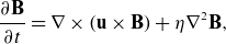 \begin{align} \dfrac {\partial \mathbf B}{\partial t} &= \nabla \times \left ( \mathbf{u} \times \mathbf{B} \right ) + \eta \nabla ^2\mathbf{B} ,\\[-10pt]\nonumber \end{align}
which comprise the solenoidality condition for the velocity, $\mathbf{u}$
and the magnetic field,
$\mathbf{u}$
and the magnetic field, $\mathbf{B}$
, and the evolution equations for the vorticity (from the momentum equation) and the magnetic field (the induction equation), respectively. Here,
$\mathbf{B}$
, and the evolution equations for the vorticity (from the momentum equation) and the magnetic field (the induction equation), respectively. Here, $\eta$
is the magnetic diffusivity, which quantifies the rate at which magnetic field lines diffuse through the plasma due to finite electrical conductivity. Notice here that we are working in Alfvén units, that is, units wherein the plasma density,
$\eta$
is the magnetic diffusivity, which quantifies the rate at which magnetic field lines diffuse through the plasma due to finite electrical conductivity. Notice here that we are working in Alfvén units, that is, units wherein the plasma density, $\rho$
, is such that
$\rho$
, is such that $4\pi \rho = 1$
.
$4\pi \rho = 1$
.
The full MHD equations (2.1–2.3) are linearized about the base states, $B_0 f\!(x)g(y)\hat {\mathbf{z}}$
in terms of the perturbed magnetic fields,
$B_0 f\!(x)g(y)\hat {\mathbf{z}}$
in terms of the perturbed magnetic fields, $ \mathbf{b}$
, and the perturbed velocity,
$ \mathbf{b}$
, and the perturbed velocity, $ \mathbf{u}$
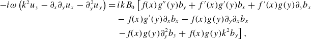
. We work with vorticity instead of the velocity field to eliminate the pressure term from the momentum equation, making the analysis simpler – one does not need to track perturbations in the pressure. The linearized vorticity equation, component-wise, yields
$ \mathbf{u}$
. We work with vorticity instead of the velocity field to eliminate the pressure term from the momentum equation, making the analysis simpler – one does not need to track perturbations in the pressure. The linearized vorticity equation, component-wise, yields
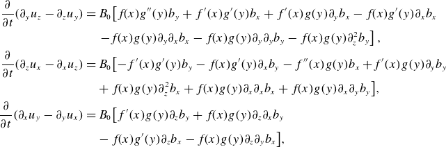 \begin{align} \dfrac {\partial }{\partial t}(\partial _y u_z - \partial _z u_y) & = B_0 \!\left[f\!(x)g^{\prime\prime}(y)b_y + f^{\prime}(x)g^{\prime}(y)b_x+ f^{\prime}(x)g(y)\partial _yb_x - f\!(x)g^{\prime}(y)\partial _xb_x \right.\nonumber\\ & \quad \left. -f\!(x)g(y)\partial _y\partial _xb_x-f\!(x)g(y)\partial _y\partial _yb_y-f\!(x)g(y) \partial _z^2b_y\right ], \nonumber \\ \dfrac {\partial }{\partial t}\!\left (\partial _z u_x - \partial _x u_z\right ) & = B_0 \big [{-}f^{\prime}(x)g^{\prime}(y)b_y - f\!(x)g^{\prime}(y)\partial _xb_y - f^{\prime\prime}(x)g(y)b_x +\! f^{\prime}(x)g(y)\partial _yb_y\nonumber\\ & \quad +f\!(x)g(y) \partial _z^2b_x +f\!(x)g(y)\partial _x\partial _xb_x +f\!(x)g(y)\partial _x\partial _yb_y\big ], \nonumber \\ \dfrac {\partial }{\partial t}(\partial _x u_y - \partial _y u_x) & = B_0 \big [ f^{\prime}(x)g(y) \partial _zb_y+ f\!(x)g(y) \partial _z\partial _xb_y \nonumber\\ & \quad - f\!(x)g^{\prime}(y)\partial _zb_x- f\!(x)g(y)\partial _z\partial _yb_x\big ], \end{align}
and the linearized induction equation, component-wise, is given by
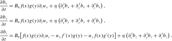 \begin{align} \dfrac {\partial b_x}{\partial t} & = B_0 f\!(x)g(y)\partial _z u_x + \eta \left ( \partial _x^2 b_x + \partial _y^2 b_x + \partial _z^2 b_x \right ),\nonumber \\[5pt] \dfrac {\partial b_y}{\partial t} & = B_0 f\!(x)g(y)\partial _z u_y + \eta \left ( \partial _x^2 b_y + \partial _y^2 b_y + \partial _z^2 b_y \right ),\nonumber \\[5pt] \dfrac {\partial b_z}{\partial t} &= B_0 \big [ f\!(x)g(y)\partial _z u_z-u_xf^{\prime}(x)g(y)-u_yf\!(x)g^{\prime}(y)\big ] + \eta \left ( \partial _x^2 b_z + \partial _y^2 b_z + \partial _z^2 b_z \right ). \end{align}
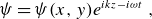
We assume that any perturbed quantity is of the form
 \begin{align} \psi = \psi (x,y) e^{ikz - i\omega t} \ , \end{align}
where $\psi$
is a placeholder for either the perturbed magnetic field or the perturbed velocity, and
$\psi$
is a placeholder for either the perturbed magnetic field or the perturbed velocity, and $\omega$
and
$\omega$
and $k$
are the frequency and the wavenumber of the perturbation along
$k$
are the frequency and the wavenumber of the perturbation along $z$
. Using this ansatz, and the solenoidality conditions for the magnetic field and the velocity, we obtain
$z$
. Using this ansatz, and the solenoidality conditions for the magnetic field and the velocity, we obtain
 \begin{align} {-i\omega }\left ( k^2 u_y-\partial _x\partial _y u_x - \partial _y^2 u_y\right ) & = ikB_0 \left[ f\!(x)g^{\prime\prime}(y)b_y + f^{\prime}(x)g^{\prime}(y)b_x + f^{\prime}(x)g(y)\partial _yb_x \right.\nonumber\\& \quad - f\!(x)g^{\prime}(y) \partial _xb_x -f\!(x)g(y)\partial _y\partial _xb_x \nonumber\\ & \quad \left. -f\!(x)g(y)\partial _y^2b_y+f\!(x)g(y) k^2b_y \right],\\[-10pt]\nonumber \end{align}
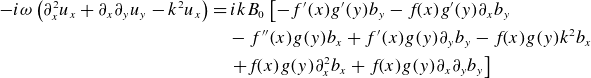 \begin{align} -i\omega \left (\partial _x^2 u_x +\partial _x\partial _y u_y-k^2 u_x \right )& = ikB_0 \left[{-}f^{\prime}(x)g^{\prime}(y)b_y - f\!(x)g^{\prime}(y)\partial _xb_y\right.\nonumber\\ & \quad - f^{\prime\prime}(x)g(y)b_x + f^{\prime}(x)g(y)\partial _yb_y -f\!(x)g(y) k^2b_x \nonumber\\ & \quad \left. +f\!(x)g(y)\partial _x^2b_x+ f\!(x)g(y)\partial _x\partial _yb_y\right]\\[-10pt]\nonumber \end{align}
 \begin{align} -i\omega b_x & = ikB_0f\!(x)g(y) u_x + \eta \left (\partial _x^2 b_x +\partial _y^2 b_x -k^2 b_x\right ) ,\\[-10pt]\nonumber \end{align}
 \begin{align} -i\omega b_y & = ikB_0f\!(x)g(y) u_y + \eta \left (\partial _x^2 b_y +\partial _y^2 b_y -k^2 b_y\right ),\\[-10pt]\nonumber \end{align}
where (2.7) and (2.8) are obtained from the linearized vorticity equations and (2.9) and (2.10) are obtained from the linearized induction equations respectively. Notice that $u_z$
and
$u_z$
and $b_z$
have been eliminated with the help of the solenoidality conditions.
$b_z$
have been eliminated with the help of the solenoidality conditions.
2.1. Analytical approach to LSA
We adopt the approach in Goldston & Rutherford (Reference Goldston and Rutherford1995) for further analysis. The main thing we focus on here is the derivation of the growth rate. The usual tearing mode analysis involves a boundary value problem. The current sheet is divided into three regions, the inner, the outer and the overlap regions. Resistive and inertial effects are negligible in the outer region and become important in the inner region where the resonant surface of $\mathbf{k}\cdot \mathbf{B}=0$
occurs and
$\mathbf{k}\cdot \mathbf{B}=0$
occurs and $f\!(x)\approx x$
. All of this follows for the 3-D case as well. The outer region equations can be used to completely characterize the instability parameter
$f\!(x)\approx x$
. All of this follows for the 3-D case as well. The outer region equations can be used to completely characterize the instability parameter
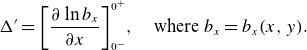 \begin{equation} \Delta^{\prime} = {\left[ \frac {\partial \ln {b_x}}{\partial x} \right]}^{0^+}_{0^-}, \quad \text{where }b_x=b_x(x,y) \text{.} \end{equation}
We will take the $\Delta ^{\prime}(y)$
as a given and proceed to examine the inner region equations which lead us to the growth rate of the 3-D instability. From (2.16), we can obtain an expression for
$\Delta ^{\prime}(y)$
as a given and proceed to examine the inner region equations which lead us to the growth rate of the 3-D instability. From (2.16), we can obtain an expression for $\partial _x^2 b_x$
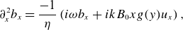 \begin{equation} \partial _x^2 b_x = \frac {-1}{\eta } \left ( i\omega b_x + ik B_0 x g(y)u_x\right ) , \end{equation}
where we have applied the standard considerations of $\partial _x^2 \gg k^2$
and
$\partial _x^2 \gg k^2$
and $f\!(x)\approx x$
in the inner region. Further, we have assumed
$f\!(x)\approx x$
in the inner region. Further, we have assumed $\partial _x^2 \gg \partial _y^2$
(see Appendix A.1 for details) and thus dropped the corresponding term as well. Next we substitute the above into (2.14) to obtain
$\partial _x^2 \gg \partial _y^2$
(see Appendix A.1 for details) and thus dropped the corresponding term as well. Next we substitute the above into (2.14) to obtain
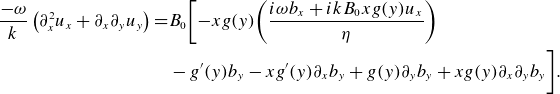 \begin{align} \frac {-\omega }{k} \left ( \partial _x^2 u_x + \partial _x\partial _y u_y \right ) =& B_0 \bigg[{-}x g(y) \bigg( \frac {i\omega b_x + ik B_0 x g(y)u_x}{\eta }\bigg) \notag \\ & - g^{\prime}(y)b_y - xg^{\prime}(y)\partial _xb_y + g(y)\partial _yb_y + xg(y)\partial _x\partial _yb_y \bigg]. \end{align}
We make an estimate of the characteristic length and velocity scales in the inner layer. First we balance first term on the left-hand side with the second one from the right-hand side of the equation above, as one would have done in the 2-D case as well. We can obtain the characteristic width of the inner resistive layer
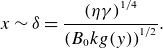 \begin{equation} x \sim \delta = \frac {\left (\eta \gamma \right )^{1/4}}{\left (B_0k g(y)\right )^{1/2}}. \end{equation}
Here, we have taken $\gamma \equiv -i\omega$
for growing modes.
$\gamma \equiv -i\omega$
for growing modes.
Next, we make the ansatz that $b_x \sim \mathrm{const.} = \tilde {b}_x$
in the inner region. This ansatz is justified easily in the 2-D case by showing that solutions of the kind
$b_x \sim \mathrm{const.} = \tilde {b}_x$
in the inner region. This ansatz is justified easily in the 2-D case by showing that solutions of the kind $b_x \propto x^n$
(where
$b_x \propto x^n$
(where $n \geqslant 1$
) are excluded (see § 20.3 in Goldston & Rutherford Reference Goldston and Rutherford1995); turns out it can be extended to the 3-D case as well. Balancing the first two terms on the right-hand side of (2.13), leads to the velocity scale
$n \geqslant 1$
) are excluded (see § 20.3 in Goldston & Rutherford Reference Goldston and Rutherford1995); turns out it can be extended to the 3-D case as well. Balancing the first two terms on the right-hand side of (2.13), leads to the velocity scale
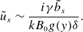 \begin{equation} \tilde {u}_x \sim \frac {i\gamma \tilde {b}_x}{kB_0 g(y) \delta } .\end{equation}
Now, we integrate (2.12) over the inner layer, so that we have
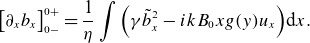 \begin{equation} \big[\partial _x b_x\big]_{0-}^{0+} = \frac {1}{\eta } \int \Big( \gamma \tilde {b}_x^2 - ik B_0 x g(y) u_x \Big) {\rm d}x. \end{equation}
With Equations (2.14) and (2.15), we can transform the variables, $X \equiv x/\delta$
,
$X \equiv x/\delta$
, $V \equiv u_x/\tilde {u}_x$
and substitute into (2.16) leading to
$V \equiv u_x/\tilde {u}_x$
and substitute into (2.16) leading to
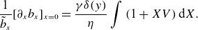 \begin{equation} \frac {1}{\tilde {b}_x}[\partial _x b_x]_{x=0} = \frac {\gamma \delta (y)}{\eta } \int \left ( 1+XV\right ) {\rm d}X. \end{equation}
The integral on the right-hand side reduces to a function that remains dependent on $y$
which we will denote as
$y$
which we will denote as $I(y)$
. And the left-hand side term is basically the instability parameter
$I(y)$
. And the left-hand side term is basically the instability parameter $\Delta ^{\prime}$
defined previously in (2.11), which for simplicity we assume to be nearly homogenous along
$\Delta ^{\prime}$
defined previously in (2.11), which for simplicity we assume to be nearly homogenous along $y$
.
$y$
.
We now substitute (2.14) into (2.17) to obtain
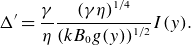 \begin{equation} \Delta ^{\prime} = \frac {\gamma }{\eta } \frac {(\gamma \eta )^{1/4}}{(kB_0 g(y))^{1/2}} I(y). \end{equation}
where $I(y)=\int (1+XV) {\rm d}X$
is still a function of
$I(y)=\int (1+XV) {\rm d}X$
is still a function of $y$
after the integration over
$y$
after the integration over $x$
. Next we re-arrange the expression and identify that
$x$
. Next we re-arrange the expression and identify that $\gamma$
needs to be independent of
$\gamma$
needs to be independent of $y$
and thus we integrate over
$y$
and thus we integrate over $y$
on both sides to obtain
$y$
on both sides to obtain
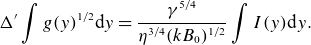 \begin{equation} \Delta ^{\prime} \int g(y)^{1/2} {\rm d}y = \frac {\gamma ^{5/4} }{\eta ^{3/4}(kB_0)^{1/2}} \int I(y) {\rm d}y. \end{equation}
Rearranging the equation, we can obtain the following dispersion relation:
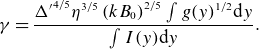 \begin{equation} \gamma = \frac {{\Delta ^{\prime}}^{4/5}\eta ^{3/5} \left ( k B_0\right )^{2/5} \int g(y)^{1/2}{\rm d}y}{\int I(y){\rm d}y}. \end{equation}
The above is quite similar to the 2-D dispersion relation obtained in the standard FKR regime (Furth et al. Reference Furth, Killeen and Rosenbluth1963) pertaining to $\Delta ^{\prime} \delta \ll 1$
, except for the integrals over
$\Delta ^{\prime} \delta \ll 1$
, except for the integrals over $y$
. We will see in a later section that, indeed, the 3-D dispersion curves inferred from direct numerical simulations do have the same behavior as in two dimensions. The main difference arises from the integrals over
$y$
. We will see in a later section that, indeed, the 3-D dispersion curves inferred from direct numerical simulations do have the same behavior as in two dimensions. The main difference arises from the integrals over $y$
and there is a reduction in the growth in this 3-D case as compared with the 2-D case by a factor of
$y$
and there is a reduction in the growth in this 3-D case as compared with the 2-D case by a factor of $\int g(y)^{1/2} {\rm d}y/\int {\rm d}y$
. Here, we have assumed that effect of modulation is negligible on the
$\int g(y)^{1/2} {\rm d}y/\int {\rm d}y$
. Here, we have assumed that effect of modulation is negligible on the $I$
integral (this would be the case if the eigen function
$I$
integral (this would be the case if the eigen function $b_x$
almost resembles its 2-D counterpart all along
$b_x$
almost resembles its 2-D counterpart all along $y$
; we show this in the next section).
$y$
; we show this in the next section).
Note that the above derivation hinges on the assumption that the modulation has a smooth or mild gradient along the third dimension. If this is not true then we cannot assume that $\Delta ^{\prime}$
is homogenous along
$\Delta ^{\prime}$
is homogenous along $y$
and effect of
$y$
and effect of $I$
integral is negligible.
$I$
integral is negligible.
In particular, it is interesting to note that the three-dimensionality of the initial equilibrium magnetic fields is such that the linear growth rate is modified from two dimensions to three dimensions by mainly a simple additional factor related to exactly the $y$
dependence (or the third direction dependence) in the initial field. This is attributed the simple nature (variable separable :
$y$
dependence (or the third direction dependence) in the initial field. This is attributed the simple nature (variable separable : $f\!(x)g(y)$
) of the extension to three dimensions. The resulting growth rate expression can be understood in the following manner.
$f\!(x)g(y)$
) of the extension to three dimensions. The resulting growth rate expression can be understood in the following manner.
If we were to extend the initial 2-D field into three dimensions with no modulation in the third direction ( $g(y)=1$
), the 2-D growth rates would be recovered. However, due to the introduction of a modulation, the strength of the magnetic field becomes non-uniform, which can affect the current sheet characteristics. In particular, we find that the characteristic length and time scales associated with the inner resistive layer are not uniform along
$g(y)=1$
), the 2-D growth rates would be recovered. However, due to the introduction of a modulation, the strength of the magnetic field becomes non-uniform, which can affect the current sheet characteristics. In particular, we find that the characteristic length and time scales associated with the inner resistive layer are not uniform along $y$
, whose effect precipitates a reduced growth rate. Again in a later section, we show that direct numerical simulations indeed confirm the growth rate reduction due to
$y$
, whose effect precipitates a reduced growth rate. Again in a later section, we show that direct numerical simulations indeed confirm the growth rate reduction due to $\int g(y)^{1/2}{\rm d}y$
.
$\int g(y)^{1/2}{\rm d}y$
.
2.2. Numerical approach to LSA
The set of equations (2.7)–(2.10) can be written as a generalized eigenvalue problem which has the form
 \begin{align} \gamma \mathcal{M} v = \mathcal{L} v, \end{align}
with $\mathcal{M}$
and
$\mathcal{M}$
and $\mathcal{L}$
are linear operators acting on the eigenfunction
$\mathcal{L}$
are linear operators acting on the eigenfunction $v$
, and
$v$
, and $\gamma$
is the corresponding eigenvalue. In our case,
$\gamma$
is the corresponding eigenvalue. In our case, $v$
comprises
$v$
comprises $u_x$
,
$u_x$
, $u_y$
,
$u_y$
, $b_x$
and
$b_x$
and $b_y$
, and we have substituted
$b_y$
, and we have substituted $\gamma = -i\omega$
in the expectation of an unstable mode with
$\gamma = -i\omega$
in the expectation of an unstable mode with $\gamma \gt 0$
.
$\gamma \gt 0$
.
We solve this generalized eigenvalue problem (EVP) numerically, using a spectral method with Fourier basis, to obtain the growth rate $\gamma$
as a function of the wavenumber
$\gamma$
as a function of the wavenumber $k$
, and the corresponding eigenfunction. The full details of the solver can be found in Appendix A.2.
$k$
, and the corresponding eigenfunction. The full details of the solver can be found in Appendix A.2.
We choose a modified Harris sheet, as the unmodulated base state, with $f\!(x) = 2.6 \tanh{\!(x)}{\textrm {sech}}^2{(x)}$
. The prefactor of
$f\!(x) = 2.6 \tanh{\!(x)}{\textrm {sech}}^2{(x)}$
. The prefactor of $2.6$
ensures that the maximum value of the magnetic field strength is
$2.6$
ensures that the maximum value of the magnetic field strength is $1$
, thus setting the Alfvénic velocity,
$1$
, thus setting the Alfvénic velocity, $v_A = 1$
, making further normalizations simpler. Notice that the base state cannot be decomposed into a finite number of Fourier modes. This can lead to truncation errors, and naively proceeding with the numerical procedure described above produces oscillatory eigenfunctions, leading to a lack of convergent solutions. To overcome this, we apply an appropriate low-pass filter (details in Appendix A.3) in Fourier space to the base state. This, by construction, gives us a base state suitable for Fourier decomposition.
$v_A = 1$
, making further normalizations simpler. Notice that the base state cannot be decomposed into a finite number of Fourier modes. This can lead to truncation errors, and naively proceeding with the numerical procedure described above produces oscillatory eigenfunctions, leading to a lack of convergent solutions. To overcome this, we apply an appropriate low-pass filter (details in Appendix A.3) in Fourier space to the base state. This, by construction, gives us a base state suitable for Fourier decomposition.
For sanity check, we first obtained the eigenfunctions for the classical tearing instability in two dimensions. In this case, we have a 1-D EVP with $v = [u_x,b_x]$
. We confirm that our method reproduces the analytically calculated eigenfunctions and the dispersion relation. This is shown in figure 1, which depicts the numerically derived eigenfunction along with the predictions of outer region theory.
$v = [u_x,b_x]$
. We confirm that our method reproduces the analytically calculated eigenfunctions and the dispersion relation. This is shown in figure 1, which depicts the numerically derived eigenfunction along with the predictions of outer region theory.
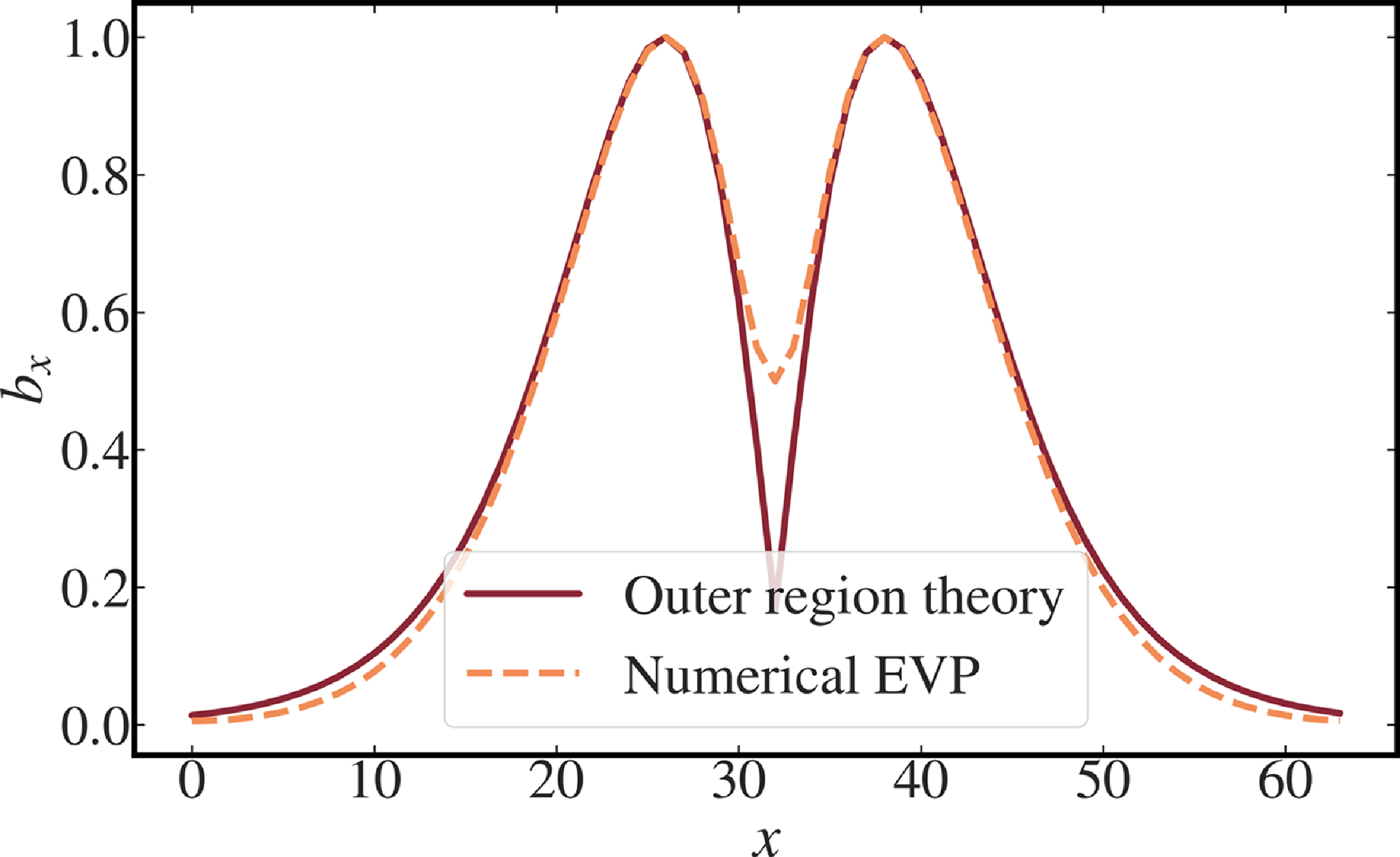
Figure 1. Match between the numerically obtained eigenfunction for the 2-D tearing instability using the EVP solver and the expectation from outer region theory.
Further, we have verified that the Fourier filtering of the equilibrium profile does not alter the dispersion relation. To establish this, we solved the EVP using a finite differencing algorithm with the unfiltered equilibrium. We did this only for the 2-D cases since a finite difference algorithm requires a greater spatial resolution owing to poor convergence and running the EVP solver using the finite differencing algorithm becomes prohibitively expensive in three dimensions.
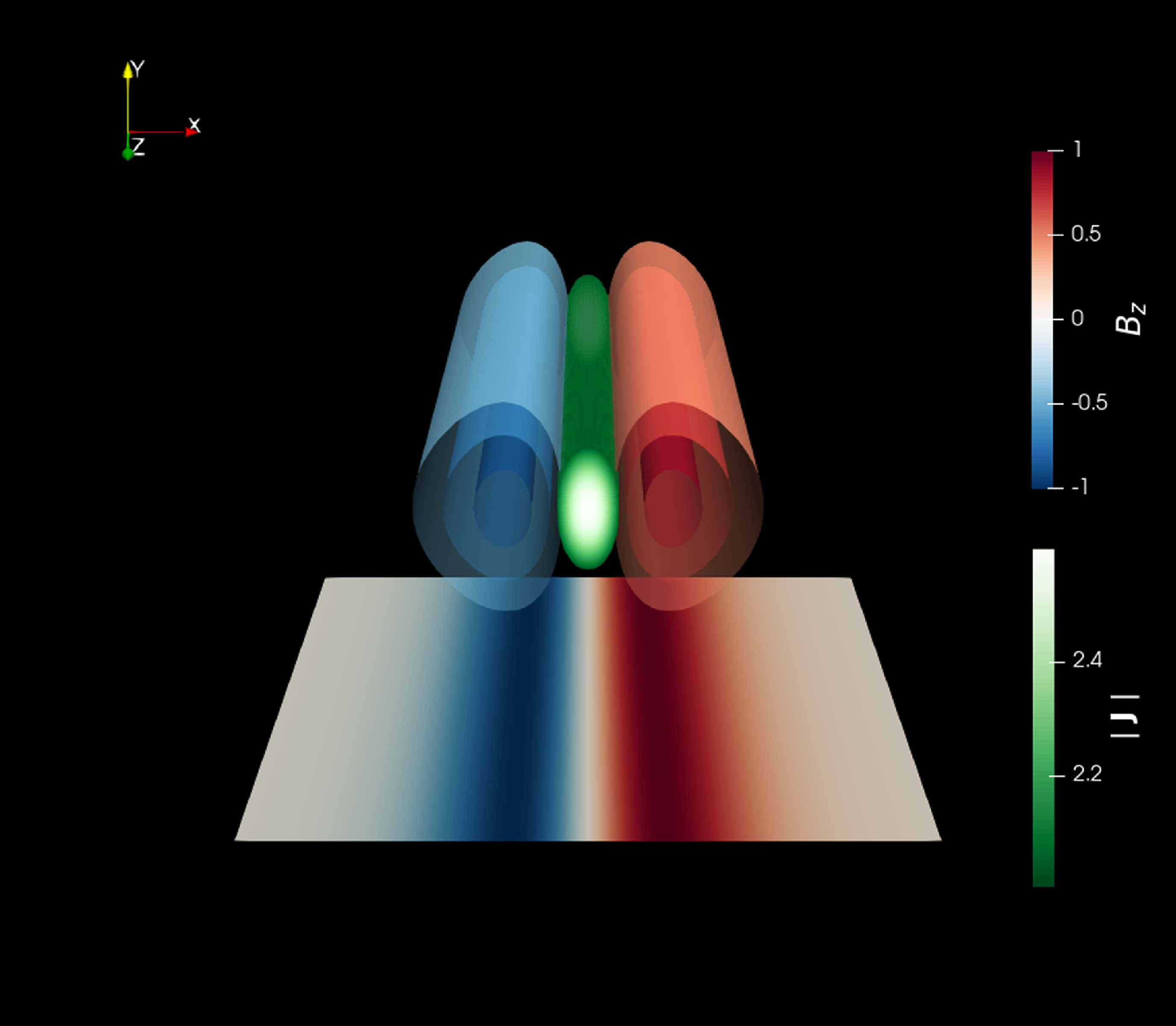
Figure 2. Equilibrium configuration of the magnetic field given by Equation (2.22) with $\lambda = 1$
. The red–blue colors show the
$\lambda = 1$
. The red–blue colors show the $z$
-component of the magnetic field and the region where the associated current density is greater than an arbitrary cutoff (
$z$
-component of the magnetic field and the region where the associated current density is greater than an arbitrary cutoff ( $\vert \mathbf{J}\vert \gt 2$
) is depicted in white–green colors. A slice of the unmodulated magnetic field is shown on the floor for comparison with the usual 2-D tearing case. Notice that the modulation provides a tubular nature to the otherwise slab-like 2-D configuration.
$\vert \mathbf{J}\vert \gt 2$
) is depicted in white–green colors. A slice of the unmodulated magnetic field is shown on the floor for comparison with the usual 2-D tearing case. Notice that the modulation provides a tubular nature to the otherwise slab-like 2-D configuration.
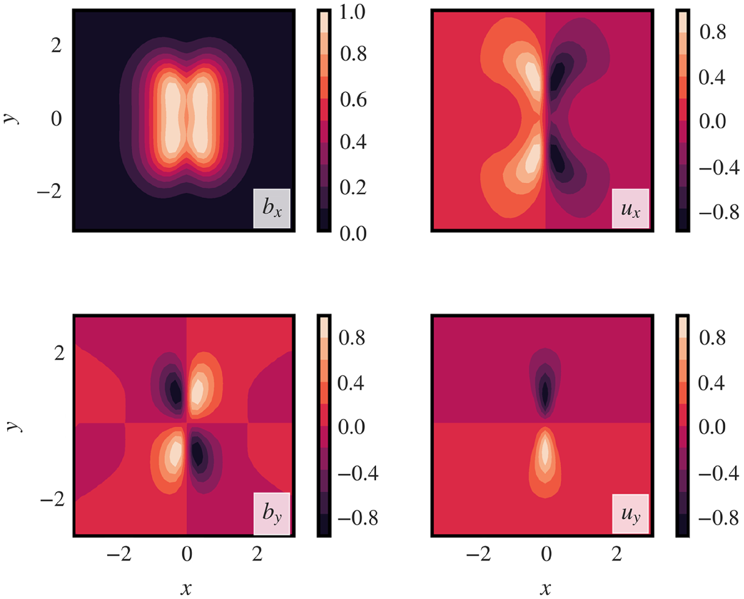
Figure 3. Eigenfunctions obtained from the numerical solution of the generalized EVP with $\eta = 0.01$
and
$\eta = 0.01$
and $k=0.7$
. Since the eigenfunctions can only be calculated up to a scale, these were rescaled to have a spatial maximum of
$k=0.7$
. Since the eigenfunctions can only be calculated up to a scale, these were rescaled to have a spatial maximum of $1$
.
$1$
.
We now present the results incorporating the modulation, $g(y)$
into the equilibrium configuration. We choose
$g(y)$
into the equilibrium configuration. We choose $g(y) = {\textrm {sech}}^2{(y/\lambda )}$
, thus modifying the equilibrium to
$g(y) = {\textrm {sech}}^2{(y/\lambda )}$
, thus modifying the equilibrium to
 \begin{equation} \mathbf{B} = f\!(x)g(y) = 2.6 \tanh {\!(x)}\, {\textrm{sech}}^2{(x)}\, {\textrm{sech}}^2{(y/\lambda )} \hat {\mathbf{z}} \text{.} \end{equation}
The magnetic field and the current configuration arising from such a profile are shown in figure 2. The parameter $\lambda$
controls the width of the modulation. An important length scale in the problem is the magnetic shear length
$\lambda$
controls the width of the modulation. An important length scale in the problem is the magnetic shear length $ a$
, over which the field reverses, typically defined as
$ a$
, over which the field reverses, typically defined as $ B_z = f(x/a)$
. Since we do not vary
$ B_z = f(x/a)$
. Since we do not vary $ a$
in this work, we set
$ a$
in this work, we set $ a = 1$
and use it to normalize all lengths throughout the analysis. As we demonstrate in the next section, this set-up closely mimics a system of reversing magnetic flux tubes with fields aligned along their axes.
$ a = 1$
and use it to normalize all lengths throughout the analysis. As we demonstrate in the next section, this set-up closely mimics a system of reversing magnetic flux tubes with fields aligned along their axes.
Figure 3 illustrates the eigenfunctions computed for a particular set of parameters, $\eta =0.01$
and
$\eta =0.01$
and $k=0.7$
. The spatial domain was taken as
$k=0.7$
. The spatial domain was taken as $(x, y) \in [-\pi , \pi ) \times [-\pi , \pi )$
and we chose
$(x, y) \in [-\pi , \pi ) \times [-\pi , \pi )$
and we chose $N_x=N_y=64$
. The velocity eigenfunctions reveal flow fields converging at the origin, coinciding with the maximum equilibrium current density. The
$N_x=N_y=64$
. The velocity eigenfunctions reveal flow fields converging at the origin, coinciding with the maximum equilibrium current density. The $x$
-component of the perturbed magnetic field exhibits a double-humped profile, reminiscent of the purely 2-D case, while the
$x$
-component of the perturbed magnetic field exhibits a double-humped profile, reminiscent of the purely 2-D case, while the $y$
-component of the magnetic field shows a quadrupolar structure.
$y$
-component of the magnetic field shows a quadrupolar structure.
The full dispersion relation, as calculated using the eigenvalue solver, is shown in figure 4. Interestingly, the dispersion relations for the 3-D cases (finite $\lambda$
) bear close resemblance to the 2-D dispersion curve, as expected from the theoretical considerations in § 2.1. One must note here that the instability parameter
$\lambda$
) bear close resemblance to the 2-D dispersion curve, as expected from the theoretical considerations in § 2.1. One must note here that the instability parameter $\Delta ^ \prime$
in the 3-D case is calculated using the same formula as in two dimensions. This is done in order to facilitate a comparison between the 2-D and 3-D cases. The measured growth rates in the 3-D cases, however, are smaller than their 2-D counterparts. Although the growth rate in three dimensions is smaller than that in two dimensions for any given wavenumber, the shape and the asymptotic scaling of the dispersion relation is similar in both cases.
$\Delta ^ \prime$
in the 3-D case is calculated using the same formula as in two dimensions. This is done in order to facilitate a comparison between the 2-D and 3-D cases. The measured growth rates in the 3-D cases, however, are smaller than their 2-D counterparts. Although the growth rate in three dimensions is smaller than that in two dimensions for any given wavenumber, the shape and the asymptotic scaling of the dispersion relation is similar in both cases.
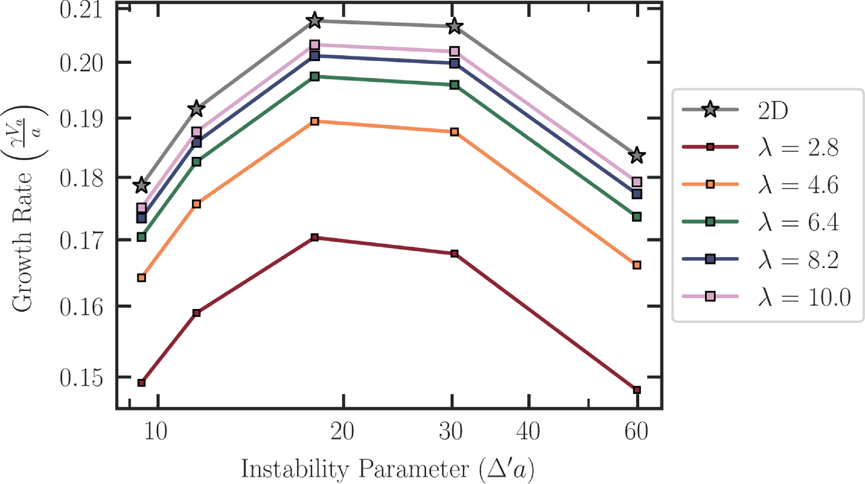
Figure 4. Dispersion curves with varying values of the modulation width $\lambda$
.
$\lambda$
.
We validate these findings by performing direct numerical simulations in § 3, and also highlight the impact of modulation on the reconnection dynamics, including the scaling of growth rates and changes in the reconnection morphology.
3. Direct numerical simulations (DNS)
We perform simulations in both two and three dimensions to obtain the corresponding dispersion relations. The 2-D simulations are necessary to validate the code by recovering the well-known tearing dispersion relation, and to have a benchmark for comparison with the 3-D results.
3.1. Numerical set-up
The initial magnetic field configuration is described by (2.22). Since this configuration is free of magnetic tension, we ensure equilibrium by choosing a suitable profile for the gas pressure, $p_{\mathrm{gas}}$
, obtained by setting
$p_{\mathrm{gas}}$
, obtained by setting $p_{\mathrm{gas}} + p_{\mathrm{mag}} = \text{const}$
, where
$p_{\mathrm{gas}} + p_{\mathrm{mag}} = \text{const}$
, where $p_{\mathrm{mag}} = B^2/2$
is the magnetic pressure. The fluid is perfectly stationary to begin with. The Lundquist number,
$p_{\mathrm{mag}} = B^2/2$
is the magnetic pressure. The fluid is perfectly stationary to begin with. The Lundquist number, $S$
can now be defined using a combination of the shear length,
$S$
can now be defined using a combination of the shear length, $a=1$
, the Alfvénic velocity,
$a=1$
, the Alfvénic velocity, $v_A = 1$
and the resistivity,
$v_A = 1$
and the resistivity, $\eta$
as
$\eta$
as $S=v_A a / \eta$
. And the Alfvénic time scale is
$S=v_A a / \eta$
. And the Alfvénic time scale is $\tau _A = a/v_A$
.
$\tau _A = a/v_A$
.
To initiate the instability, perturbations of the form $b_x = \sin (k^* z)$
are introduced in the
$b_x = \sin (k^* z)$
are introduced in the $x$
component of the magnetic field. For a given simulation, we introduce perturbations of only a single wavenumber,
$x$
component of the magnetic field. For a given simulation, we introduce perturbations of only a single wavenumber, $k^*$
, in the
$k^*$
, in the $z$
direction. This is done to estimate growth rates mode by mode, as is required to obtain the dispersion relation. Introducing perturbations with a multitude of wavenumbers would lead to the observation of only the fastest-growing mode, and one would not be able to get the dispersion relation.
$z$
direction. This is done to estimate growth rates mode by mode, as is required to obtain the dispersion relation. Introducing perturbations with a multitude of wavenumbers would lead to the observation of only the fastest-growing mode, and one would not be able to get the dispersion relation.
We use a pseudo-spectral code, written using the Dedalus framework (Burns et al. Reference Burns, Vasil, Oishi, Lecoanet and Brown2020), to solve the usual visco-resistive MHD equations. The spectral expansion is done in Fourier basis which translates to periodic boundary conditions in all directions for both the 2-D and the 3-D cases. We work with a resolution of $N_x = 128$
,
$N_x = 128$
, $N_y = 128$
and
$N_y = 128$
and $N_z = 64$
, and the box size is
$N_z = 64$
, and the box size is $L_x = 4\pi$
,
$L_x = 4\pi$
, $L_y = 4\pi$
and
$L_y = 4\pi$
and $L_z = 2\pi /k^*$
. This choice of
$L_z = 2\pi /k^*$
. This choice of $L_z$
ensures that the perturbation of wavenumber
$L_z$
ensures that the perturbation of wavenumber $k^*$
fits exactly in the box. As in § 2.2, a low-pass filter is applied on the initial condition to ensure periodicity. A 3/2 dealiasing scheme is implemented to avoid aliasing errors, and time stepping is done using a second-order Runge–Kutta scheme. Convergence tests were done to ensure that the results are not affected by the resolution.
$k^*$
fits exactly in the box. As in § 2.2, a low-pass filter is applied on the initial condition to ensure periodicity. A 3/2 dealiasing scheme is implemented to avoid aliasing errors, and time stepping is done using a second-order Runge–Kutta scheme. Convergence tests were done to ensure that the results are not affected by the resolution.
Because of finite, non-zero resistivity, the base state is not in equilibrium, rather, it diffuses out, as observed in Landi et al. (Reference Landi, Londrillo, Velli and Bettarini2008). This equilibrium diffusion ( $ \eta \nabla ^2 \mathbf{B}_0$
) is usually ignored in tearing mode analysis by assuming that the time scales of this diffusion are larger than the time scales of the tearing instability. This assumption holds well in the case of very small
$ \eta \nabla ^2 \mathbf{B}_0$
) is usually ignored in tearing mode analysis by assuming that the time scales of this diffusion are larger than the time scales of the tearing instability. This assumption holds well in the case of very small $ \eta$
as is typical of astrophysical systems. However, for our modest values of the Lundquist number, we find that the equilibrium diffusion time scale is comparable to the tearing instability time scale. This is especially true for the 3-D case, where the equilibrium diffusion time scale is even smaller. This equilibrium diffusion leads to a slow decay of the base state, and so the linear regime of growth is not sustained for long in our fully nonlinear simulations. To circumvent this, following Landi et al. (Reference Landi, Londrillo, Velli and Bettarini2008), we add a constant term to the induction equation,
$ \eta$
as is typical of astrophysical systems. However, for our modest values of the Lundquist number, we find that the equilibrium diffusion time scale is comparable to the tearing instability time scale. This is especially true for the 3-D case, where the equilibrium diffusion time scale is even smaller. This equilibrium diffusion leads to a slow decay of the base state, and so the linear regime of growth is not sustained for long in our fully nonlinear simulations. To circumvent this, following Landi et al. (Reference Landi, Londrillo, Velli and Bettarini2008), we add a constant term to the induction equation, $-\eta \nabla ^2 \mathbf{B}_0$
, that rules out the equilibrium diffusion. This ensures that the base state does not decay and the tearing instability can be studied in the linear regime.
$-\eta \nabla ^2 \mathbf{B}_0$
, that rules out the equilibrium diffusion. This ensures that the base state does not decay and the tearing instability can be studied in the linear regime.
4. Simulation results
The evolution of the magnetic field driven by the 3-D tearing instability is illustrated in figure 5. The initially flux-tube-like magnetic fields converge, break and reconnect to create new flux tubes. The behavior of these flux tubes closely resembles the dynamics of field lines observed in the 2-D tearing instability.
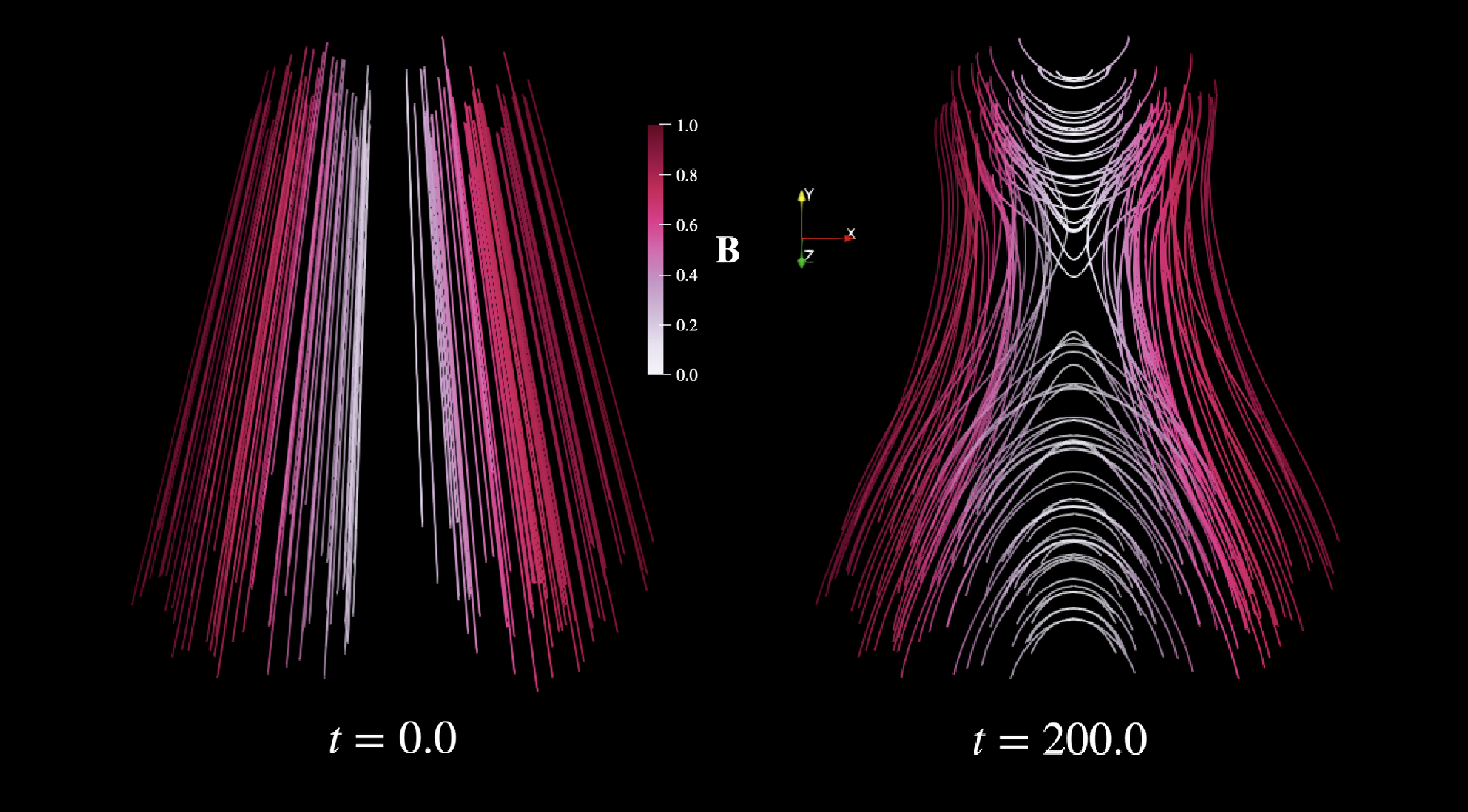
Figure 5. Streamlines of the magnetic field. The left figure shows the initial configuration and the flux-tube-like structure is clearly visible. The structure at a later time is shown on the right. The color represents the magnitude of the magnetic field.
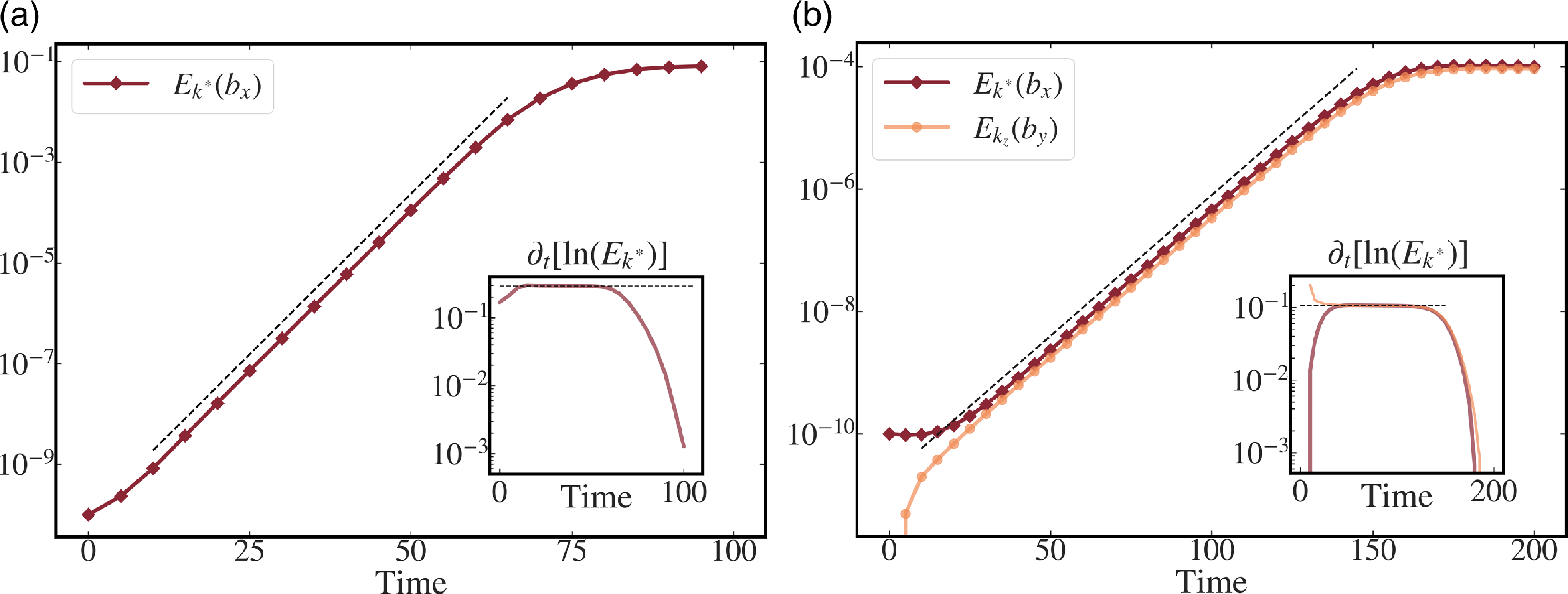
Figure 6. Growth of perturbations in the 2-D case (left) and the 3-D case (right). The plot shows the linear growth of the energy in the unstable mode, $E_{k^*}$
, vs time (given in code units). The inset shows the evolution of the local slope, depicting a clean linear growth phase where the slope is a constant in time. The dashed line shows the fitted growth rate in both the plots.
$E_{k^*}$
, vs time (given in code units). The inset shows the evolution of the local slope, depicting a clean linear growth phase where the slope is a constant in time. The dashed line shows the fitted growth rate in both the plots.
The growth rate of the instability is measured by tracking the spectral energy in the $x$
and the
$x$
and the $y$
components of the magnetic field for
$y$
components of the magnetic field for $k = k^*$
. This is given by
$k = k^*$
. This is given by
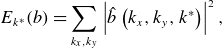 \begin{align} E_{k^*}(b)=\sum\limits_{k_{x},k_y}\left |\hat {b}\left (k_{x},k_y,k^*\right ) \right |^{2} , \end{align}
where $b$
represents the
$b$
represents the $x$
or
$x$
or $y$
component of the magnetic field,
$y$
component of the magnetic field, $\hat {b}$
is the corresponding Fourier transform and the summation is taken over all wavenumbers in the
$\hat {b}$
is the corresponding Fourier transform and the summation is taken over all wavenumbers in the $x$
and the
$x$
and the $y$
directions. The growth rate is then calculated by taking the local slope of
$y$
directions. The growth rate is then calculated by taking the local slope of $\ln \left ({E_{k^*}}\right )$
vs time. This shows a clean linear growth phase, as shown in figure 6, where the local slope (shown in the insets) is a constant, as is expected in the linear regime of the tearing instability.
$\ln \left ({E_{k^*}}\right )$
vs time. This shows a clean linear growth phase, as shown in figure 6, where the local slope (shown in the insets) is a constant, as is expected in the linear regime of the tearing instability.
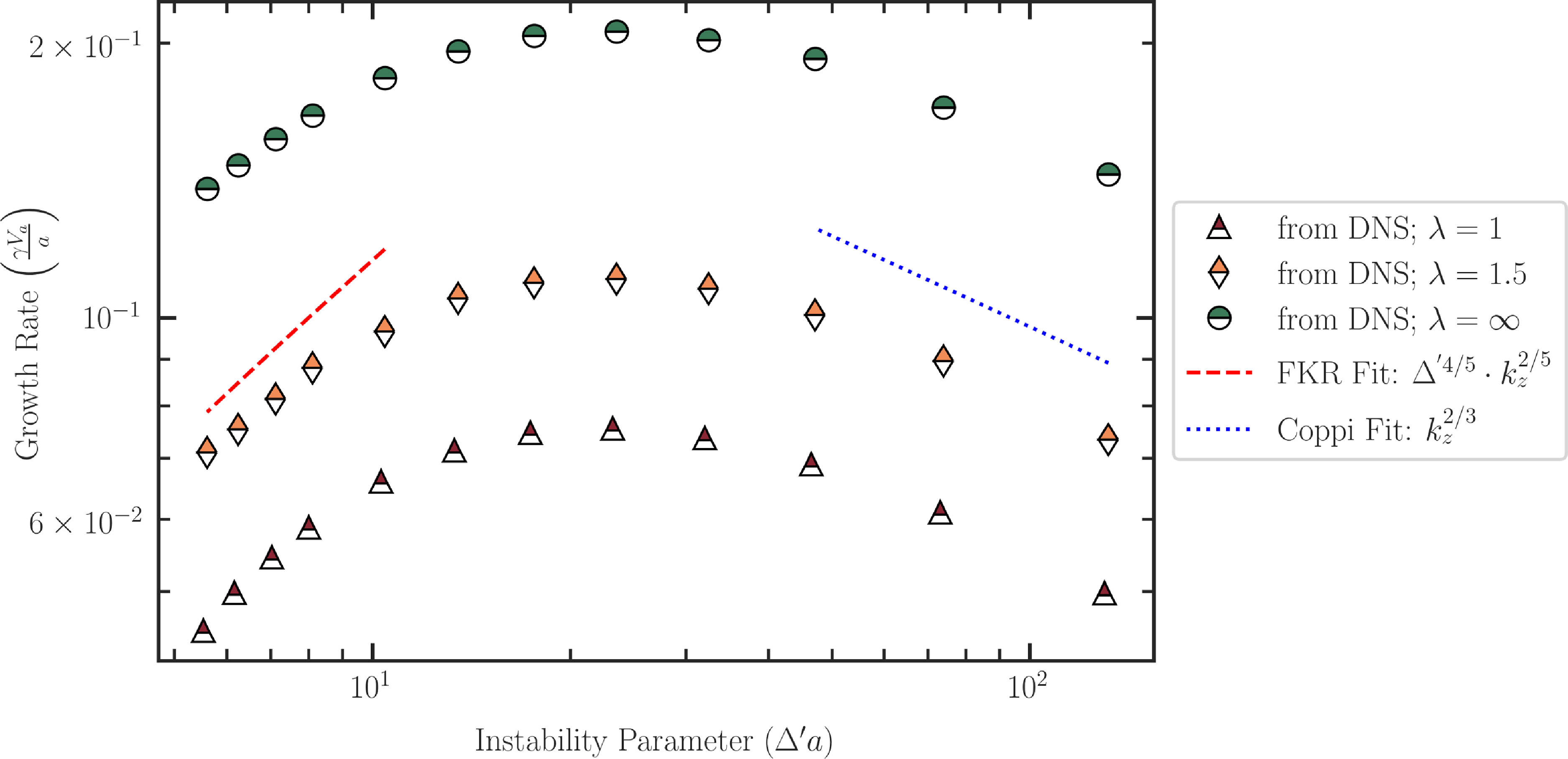
Figure 7. Dispersion relation in the 3-D case with variation in the width of the modulation, $\lambda$
. The dashed lines show the asymptotic theoretical growth rates in the FKR and the Coppi regimes, and the points are the measured growth rates. The 2-D dispersion relation with
$\lambda$
. The dashed lines show the asymptotic theoretical growth rates in the FKR and the Coppi regimes, and the points are the measured growth rates. The 2-D dispersion relation with $\lambda \rightarrow \infty$
is shown for reference.
$\lambda \rightarrow \infty$
is shown for reference.
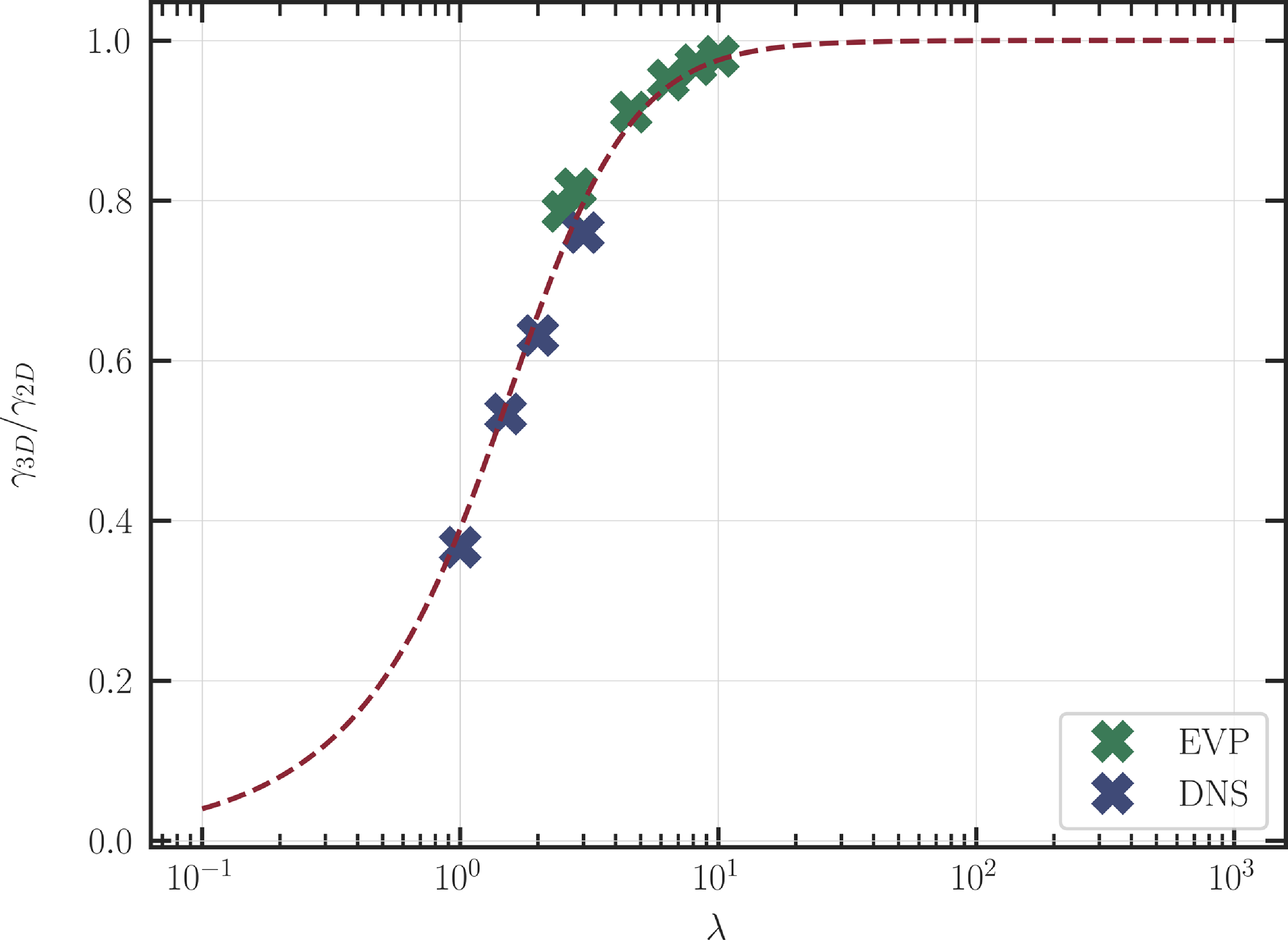
Figure 8. Effect of the modulation width $\lambda$
on the growth rate. The plot shows the ratio of the growth rate in three dimensions to that in two dimensions (or
$\lambda$
on the growth rate. The plot shows the ratio of the growth rate in three dimensions to that in two dimensions (or $\lambda =\infty$
),
$\lambda =\infty$
), $\gamma _{3D}/\gamma _{2D}$
vs. the modulation width
$\gamma _{3D}/\gamma _{2D}$
vs. the modulation width $\lambda$
, for a fixed wavenumber
$\lambda$
, for a fixed wavenumber $k^* = 0.7$
. The blue crosses are measurements from the simulations and the green ones are from the eigenvalue solver. The maroon line is the theoretical prediction using (2.20).
$k^* = 0.7$
. The blue crosses are measurements from the simulations and the green ones are from the eigenvalue solver. The maroon line is the theoretical prediction using (2.20).
The dispersion relation is obtained by measuring growth rates for different wavenumbers. These growth rates are plotted against the tearing instability parameter $\Delta ^ \prime a$
in figure 7. The theoretical growth rate scalings in the FKR (
$\Delta ^ \prime a$
in figure 7. The theoretical growth rate scalings in the FKR ( $\Delta ^ \prime \delta \ll 1$
) and the Coppi (
$\Delta ^ \prime \delta \ll 1$
) and the Coppi ( $\Delta ^ \prime \delta \sim 1$
) regimes are given in dot-dashed red and dotted blue lines, respectively. The measured dispersion curves agree well with theoretical scalings. Figure 7 reaffirms our findings in the previous sections – the growth rates in three dimensions are smaller but the shape of the dispersion curve and the fastest-growing mode are independent of the width of the modulation.
$\Delta ^ \prime \delta \sim 1$
) regimes are given in dot-dashed red and dotted blue lines, respectively. The measured dispersion curves agree well with theoretical scalings. Figure 7 reaffirms our findings in the previous sections – the growth rates in three dimensions are smaller but the shape of the dispersion curve and the fastest-growing mode are independent of the width of the modulation.
As discussed in § 2.1, the growth rates in the 3-D case are affected by the modulation, as given in (2.20). We now plot the effect of the modulation on the growth rate for a given wavenumber in figure 8. The maroon solid line shows the theoretical prediction of $\gamma$
for varying modulation width
$\gamma$
for varying modulation width $\lambda$
in
$\lambda$
in $g(y)$
using (2.20). The 3-D growth rates are reduced by a factor of
$g(y)$
using (2.20). The 3-D growth rates are reduced by a factor of $\int g(y)^{1/2}{\rm d}y/\int {\rm d}y$
from the 2-D case of
$\int g(y)^{1/2}{\rm d}y/\int {\rm d}y$
from the 2-D case of $\lambda =\infty ,\,g(y)=1$
. We find that there is indeed a good match between the growth rates obtained from the eigenvalue solver, the simulations and the theory. Further, in figure 9, we show that the dispersion curves for different
$\lambda =\infty ,\,g(y)=1$
. We find that there is indeed a good match between the growth rates obtained from the eigenvalue solver, the simulations and the theory. Further, in figure 9, we show that the dispersion curves for different $\lambda$
fall on top of each other – and the purely 2-D dispersion curve – when the measured growth rate is rescaled by the prefactor calculated in (2.20). This collapse confirms that the primary effect of the modulation is to uniformly scale the growth rate across wavenumbers, without altering the shape of the dispersion relation. It validates our theoretical prediction that the spatial variation in
$\lambda$
fall on top of each other – and the purely 2-D dispersion curve – when the measured growth rate is rescaled by the prefactor calculated in (2.20). This collapse confirms that the primary effect of the modulation is to uniformly scale the growth rate across wavenumbers, without altering the shape of the dispersion relation. It validates our theoretical prediction that the spatial variation in $g(y)$
simply attenuates the overall instability strength.
$g(y)$
simply attenuates the overall instability strength.
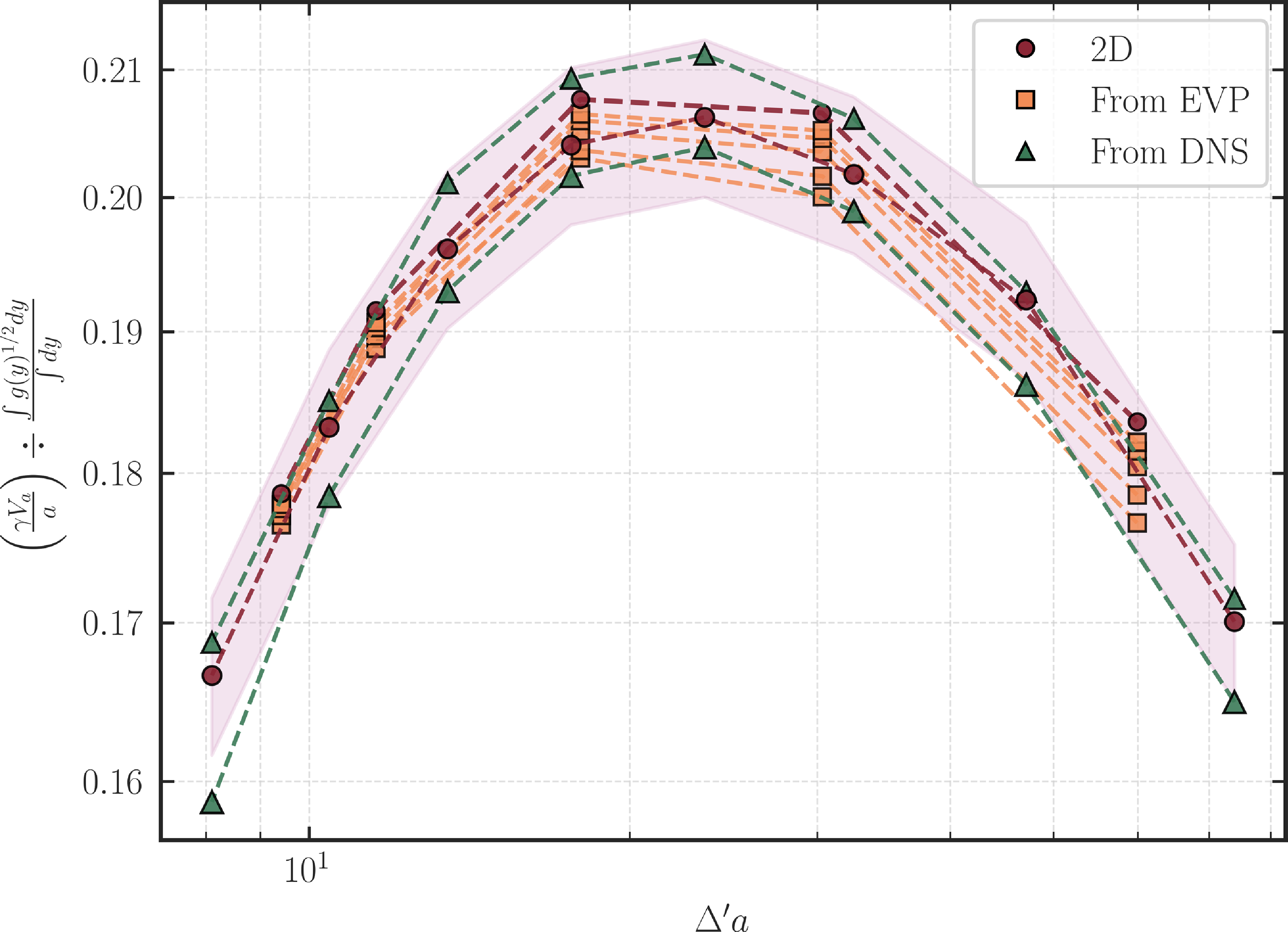
Figure 9. Collapse of the measured dispersion relation (from both the DNS and the EVP) on top of the 2-D dispersion curve when the corresponding growth rates are rescaled by the exact $\lambda$
dependent prefactor predicted in (2.20).
$\lambda$
dependent prefactor predicted in (2.20).
The magnetic field eigenfunctions can also be obtained from these fully nonlinear simulations by taking a constant $z$
slice from the simulation domain. Figure 10 shows the so obtained eigenfunctions and they are in good agreement with those obtained from the linear theory in § 2.2.
$z$
slice from the simulation domain. Figure 10 shows the so obtained eigenfunctions and they are in good agreement with those obtained from the linear theory in § 2.2.
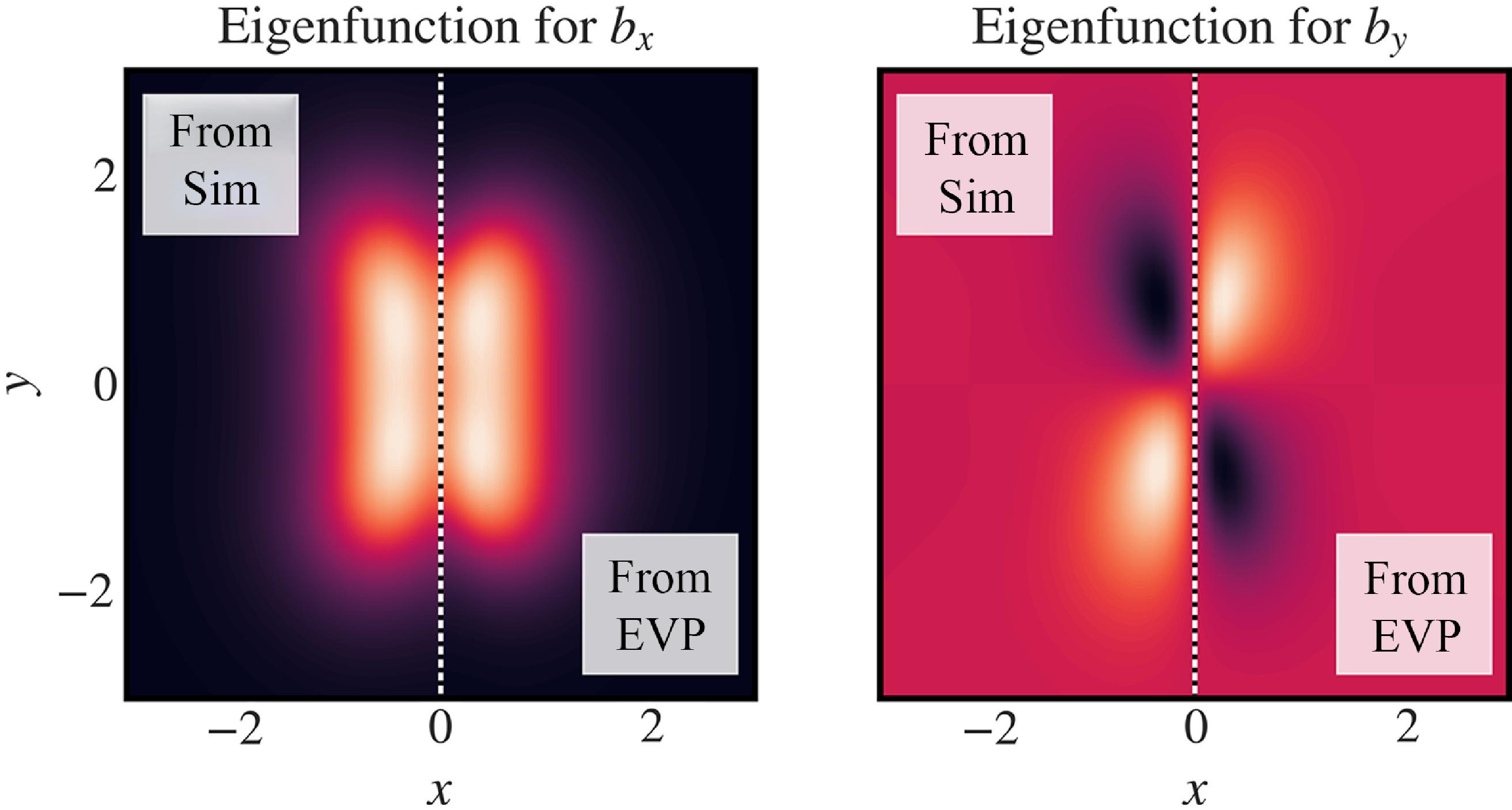
Figure 10. Comparison of the eigenfunctions obtained from the linear theory and the fully nonlinear simulations. The eigenfunctions are shown for the same parameters, $\eta = 0.01$
and
$\eta = 0.01$
and $k=0.7$
. The left plot shows the
$k=0.7$
. The left plot shows the $x$
-component of the perturbed magnetic field,
$x$
-component of the perturbed magnetic field, $b_x$
, and the plot on the right shows the
$b_x$
, and the plot on the right shows the $y$
-component of the perturbed magnetic field,
$y$
-component of the perturbed magnetic field, $b_y$
.
$b_y$
.
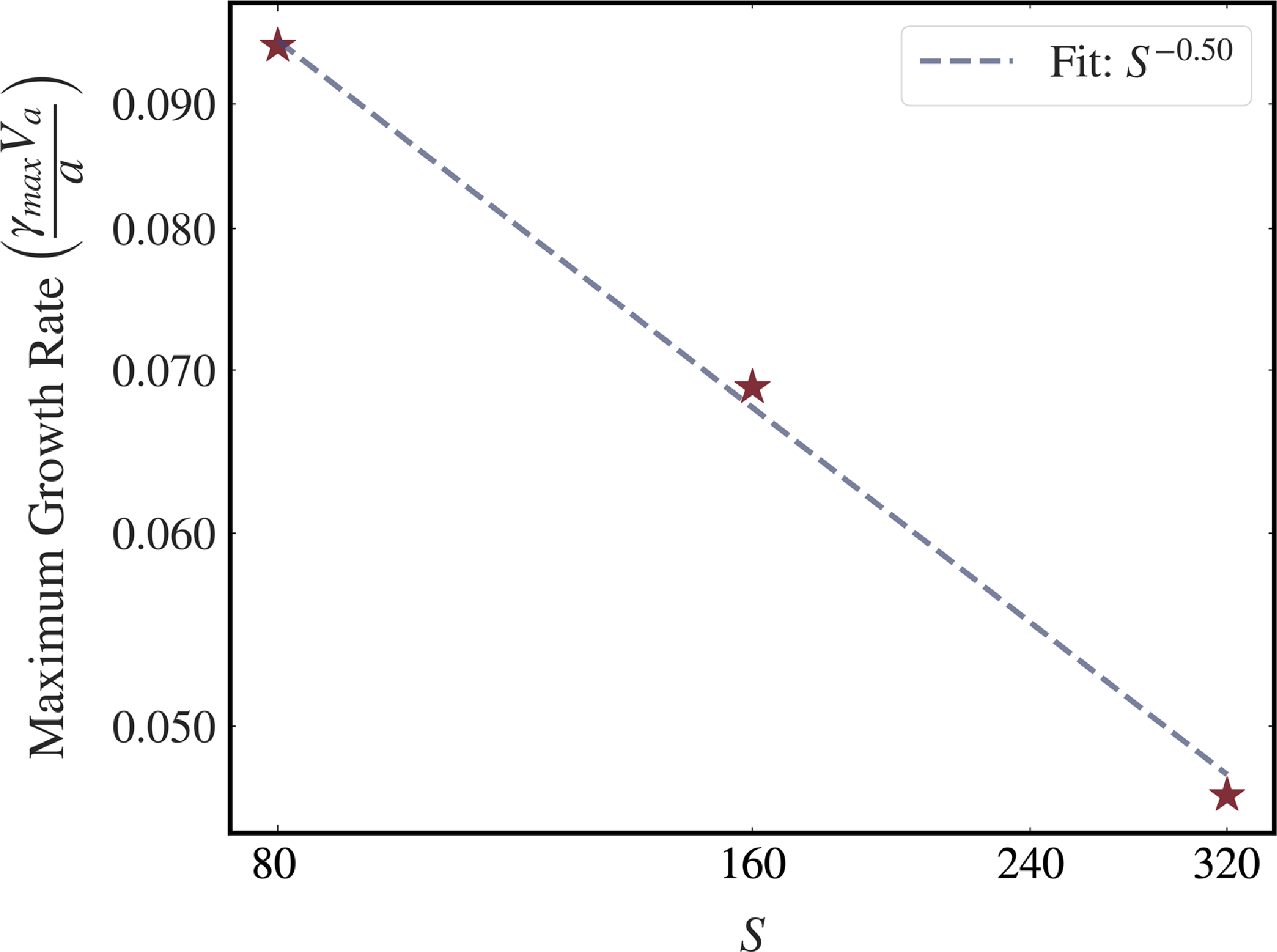
Figure 11. Scaling of the maximum growth rate with the Lundquist number $S$
. The maximum growth rate was obtained by interpolating the individual dispersion relations. The solid line, which shows the
$S$
. The maximum growth rate was obtained by interpolating the individual dispersion relations. The solid line, which shows the $S^{-1/2}$
scaling, is in good agreement with the data.
$S^{-1/2}$
scaling, is in good agreement with the data.
The Lundquist number scaling of the maximum growth rate in the 3-D case is also similar to the 2-D case. This was confirmed by performing 3 different suites of simulations with S = 80, 160 and 320, and obtaining the full dispersion relation in each case. The maximum growth rate was estimated by interpolating the obtained dispersion relation on a finer $\Delta ^{\prime}$
grid and then taking the maxima. The scaling of the maximum growth rate with the Lundquist number is shown in figure 11.
$\Delta ^{\prime}$
grid and then taking the maxima. The scaling of the maximum growth rate with the Lundquist number is shown in figure 11.
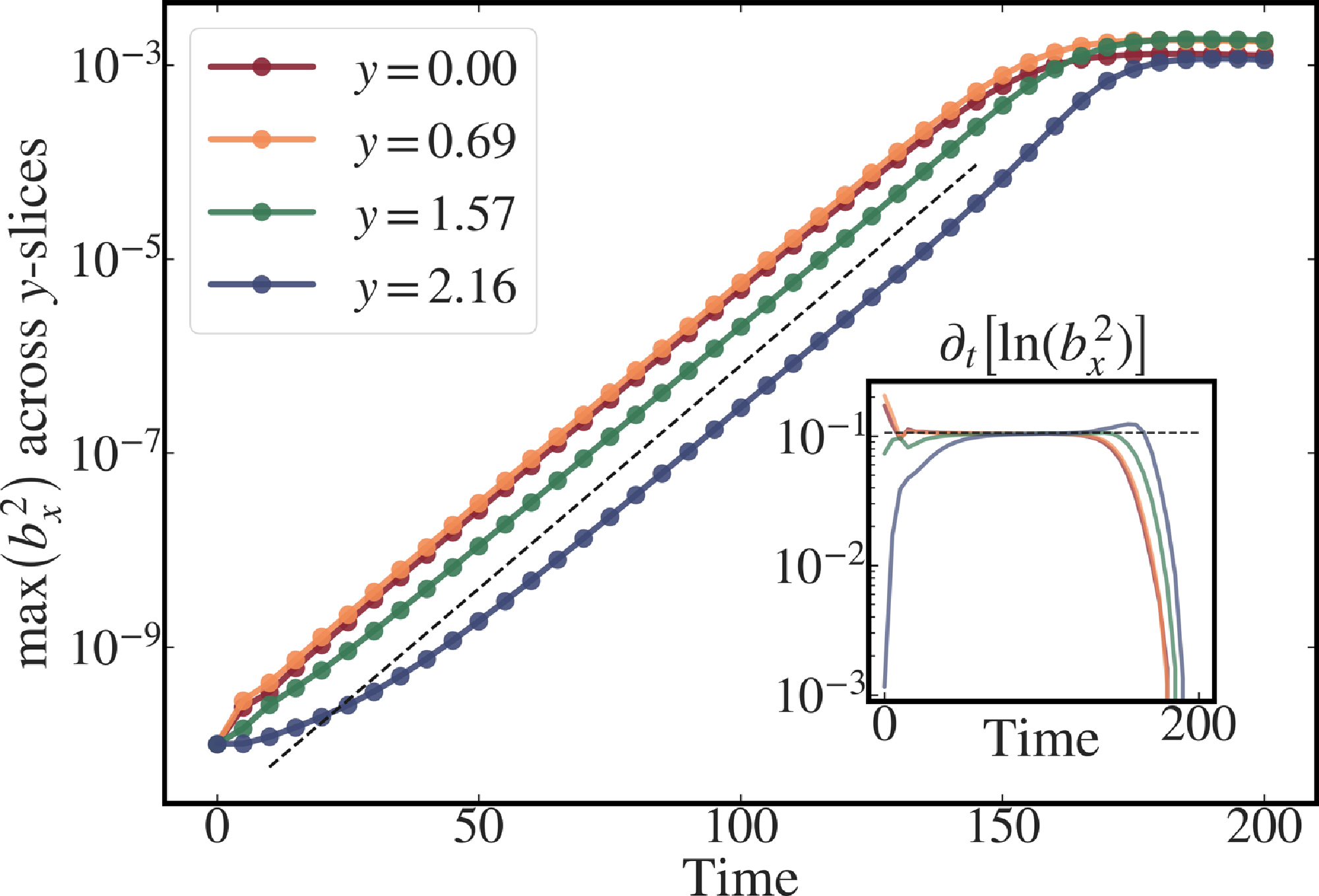
Figure 12. Growth of perturbations in different $y$
-slices. The plot shows the maximum
$y$
-slices. The plot shows the maximum $b_x^2$
across
$b_x^2$
across $y$
-slices vs time. The growth rate is the same as that obtained from the spectral energy, indicating cross-coupling between the slices.
$y$
-slices vs time. The growth rate is the same as that obtained from the spectral energy, indicating cross-coupling between the slices.
Given these similarities between the 2-D and the 3-D cases, one must question if there is any impact of the third direction, or is the 3-D case simply a stack of different 2-D tearing slices with different Alfvénic time scales, and hence different growth rates, which conspire to give a net smaller growth rate. To investigate this, we plot the growth of the perturbations in different $y$
-slices. The maximum
$y$
-slices. The maximum $b_x^2$
across
$b_x^2$
across $y$
-slices shows the same growth rate as shown in figure 12, and this growth rate is also the same as that obtained from the spectral energy. This clearly signifies that all the
$y$
-slices shows the same growth rate as shown in figure 12, and this growth rate is also the same as that obtained from the spectral energy. This clearly signifies that all the $y$
-slices have cross-coupling, and hence, the 3-D problem is not simply a stack of 2-D slices.
$y$
-slices have cross-coupling, and hence, the 3-D problem is not simply a stack of 2-D slices.
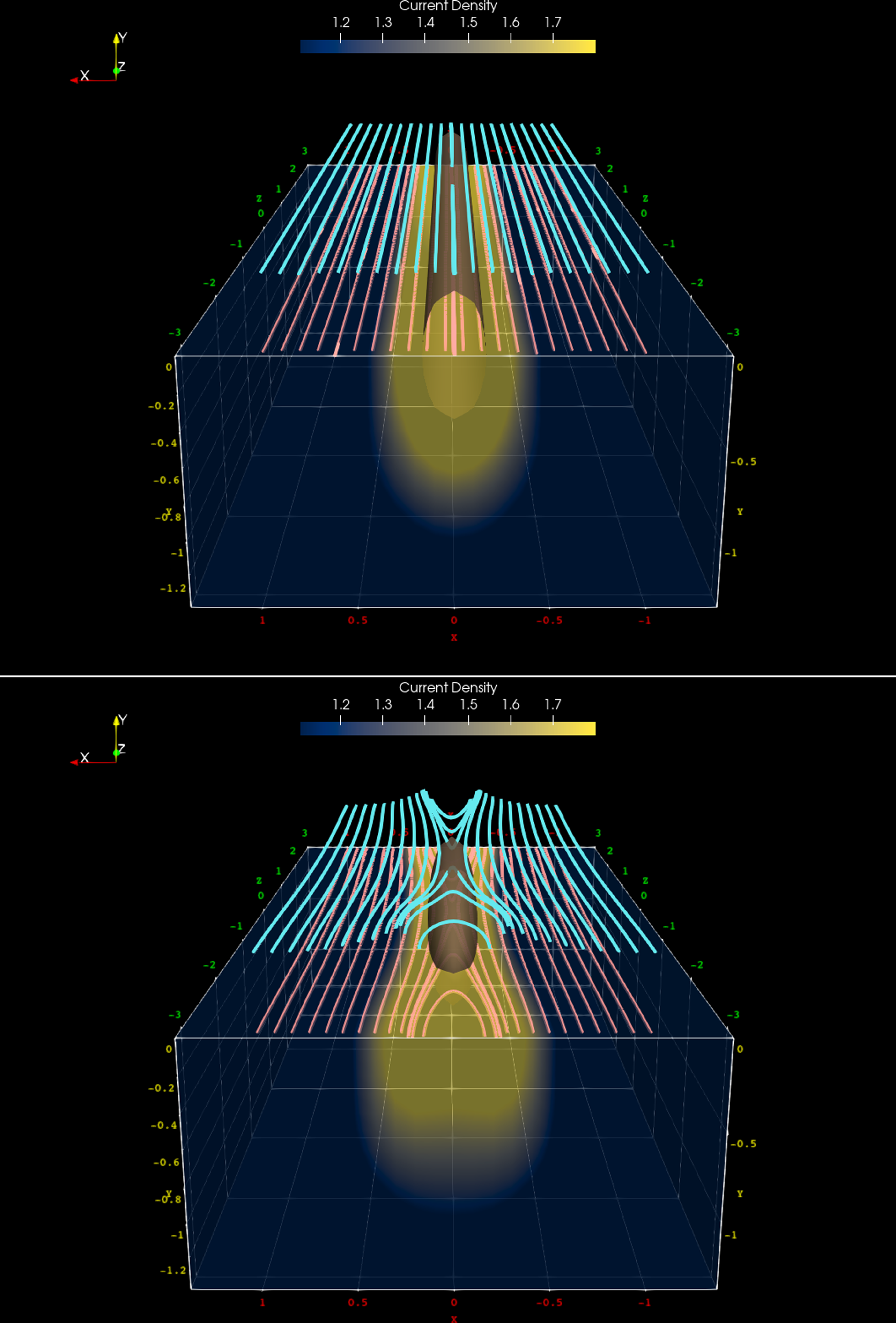
Figure 13. Magnetic field streamlines at two different times. Left: initial state. Right: state at a later time in the linear growth stage. The volume rendering shows the current density and magnetic field lines are shown in pink (in the $y=0$
plane) and in cyan (off center plane,
$y=0$
plane) and in cyan (off center plane, $y \neq 0$
). The magnetic islands away from the
$y \neq 0$
). The magnetic islands away from the $y=0$
plane appear bent in the
$y=0$
plane appear bent in the $y$
-direction.
$y$
-direction.
Next, we show in figure 13 various structures ensuing as a result of the 3-D tearing instability. The volume rendering in the figure shows the current density, $\mathbf{J}$
and an isocontour corresponding to a high value of
$\mathbf{J}$
and an isocontour corresponding to a high value of $\mathbf{J}$
is also shown in brown color. The magnetic field lines in the
$\mathbf{J}$
is also shown in brown color. The magnetic field lines in the $y=0$
plane are shown in pink, and bear close resemblance to the purely 2-D tearing instability. The cyan lines show the magnetic field in an off center plane. While these also have similarities with the 2-D case, there is a clear 3-D structure to these lines, with a finite non-zero
$y=0$
plane are shown in pink, and bear close resemblance to the purely 2-D tearing instability. The cyan lines show the magnetic field in an off center plane. While these also have similarities with the 2-D case, there is a clear 3-D structure to these lines, with a finite non-zero $y$
-component of the magnetic field leading to magnetic islands that are bent in the
$y$
-component of the magnetic field leading to magnetic islands that are bent in the $y$
-direction.
$y$
-direction.
In the purely 2-D scenario, a region of enhanced current density around an X-point with oval-shaped contours emerges along with the tearing mode and island formation. Analogously, in three dimensions, the current density contour reveals an oblong, ellipsoid-like structure as can be seen in the right-hand side plot in figure 13. Taking the analogy further, in 2-D tearing modes, the X-point draws magnetic field lines toward itself, facilitating reconnection at the X-point. This idea can also be extended to three dimensions. The pronounced current density (shown by the ellipsoid-like structure) is indicative of the magnetic null or the X-point close to the $y=0$
plane responsible for pulling of the plasma containing field lines toward itself, causing the magnetic islands to be bent in the
$y=0$
plane responsible for pulling of the plasma containing field lines toward itself, causing the magnetic islands to be bent in the $y$
-direction, and thereby giving rise to the observed 3-D structure. Please see Appendix A.4 for further details of island structures and their corresponding null points, along
$y$
-direction, and thereby giving rise to the observed 3-D structure. Please see Appendix A.4 for further details of island structures and their corresponding null points, along $y$
.
$y$
.
5. Conclusions and discussions
In this paper, we studied a 3-D extension of the tearing instability. A straightforward 3-D extension would consist of simply extending the standard 2-D equilibrium into the third dimension and allowing for 3-D perturbations. However, in such cases, the fastest-growing modes remain identical to their 2-D counterparts, as per Squire’s theorem (Squire Reference Squire1933). A more commonly explored 3-D extension includes a uniform magnetic field along the third dimension, often referred to as a guide field. If the guide field is strong, then we recover the 2-D behavior as seen in reduced MHD.
For our study, we considered a different 3-D extension involving incorporation of a simple dependence of the field on the third direction, which we refer to as a modulation i.e. the 2-D field, $B_z(x)$
was multiplied by a function,
$B_z(x)$
was multiplied by a function, $g(y)$
. In particular, we employed
$g(y)$
. In particular, we employed $B_z= \tanh (x)\,{\textrm{sech}}^2(x)\, {\textrm{sech}}^2(y/\lambda )$
, which would represent a system with reversing magnetic flux tubes.Footnote
1
This can be considered as a simplified version of the vortex tube configuration in Melander & Hussain (Reference Melander and Hussain1989).
$B_z= \tanh (x)\,{\textrm{sech}}^2(x)\, {\textrm{sech}}^2(y/\lambda )$
, which would represent a system with reversing magnetic flux tubes.Footnote
1
This can be considered as a simplified version of the vortex tube configuration in Melander & Hussain (Reference Melander and Hussain1989).
Remarkably, we have found that this 3-D equilibrium gives rise to tearing-like modes even without the presence of guide fields. Further, it turned out that this 3-D configuration is amenable to tractable linear theory analysis. We derived a testable prediction: the impact of the modulation on the growth rate. Specifically, the linear growth rate is reduced by a factor of $\int g(y)^{1/2}{\rm d}y/ \int {\rm d}y$
. This reduction is attributed to the effect of the modulation on the properties of the inner resistive layer which are not uniform along the third dimension. Essentially, the reconnection retains a topologically 2-D-like nature in such a system, but the three-dimensionality of the initial equilibrium – manifested through the modulation in the third direction – is reflected in the growth rate. It has been discussed in Pontin (Reference Pontin2011) that reconnections are fundamentally different in three dimensions as field lines are not confined to a plane. However, we find that configurations as in our work allow for reconnections plane by plane with cutting and rejoining of field lines while maintaining a unified 3-D character. In the ideal case, from the uncurled induction equation and Faraday’s law, the electric field
$\int g(y)^{1/2}{\rm d}y/ \int {\rm d}y$
. This reduction is attributed to the effect of the modulation on the properties of the inner resistive layer which are not uniform along the third dimension. Essentially, the reconnection retains a topologically 2-D-like nature in such a system, but the three-dimensionality of the initial equilibrium – manifested through the modulation in the third direction – is reflected in the growth rate. It has been discussed in Pontin (Reference Pontin2011) that reconnections are fundamentally different in three dimensions as field lines are not confined to a plane. However, we find that configurations as in our work allow for reconnections plane by plane with cutting and rejoining of field lines while maintaining a unified 3-D character. In the ideal case, from the uncurled induction equation and Faraday’s law, the electric field $\mathbf{E}$
satisfies
$\mathbf{E}$
satisfies $\mathbf{E} + \mathbf{v}\times \mathbf{B}=\mathbf{\nabla }\Phi$
. According to Pontin (Reference Pontin2011), it is possible to derive a smooth velocity field in two dimensions, as long as
$\mathbf{E} + \mathbf{v}\times \mathbf{B}=\mathbf{\nabla }\Phi$
. According to Pontin (Reference Pontin2011), it is possible to derive a smooth velocity field in two dimensions, as long as $\mathbf{E}\cdot \mathbf{B}=0$
and
$\mathbf{E}\cdot \mathbf{B}=0$
and $(\mathbf{\nabla }\Phi )\cdot \mathbf{B}=0$
, except at magnetic nulls. Thus, at X-points where the smoothness of the flow breaks down, we have reconnections. Further, they say that in three dimensions, it is not possible to have
$(\mathbf{\nabla }\Phi )\cdot \mathbf{B}=0$
, except at magnetic nulls. Thus, at X-points where the smoothness of the flow breaks down, we have reconnections. Further, they say that in three dimensions, it is not possible to have $\mathbf{E}\cdot \mathbf{B}=0$
(due to the complicated geometry of the magnetic fields) and thus the conditions for flux freezing and magnetic topology conservation are more sophisticated. However, we find that our simple 3-D reconnecting field configuration is such that
$\mathbf{E}\cdot \mathbf{B}=0$
(due to the complicated geometry of the magnetic fields) and thus the conditions for flux freezing and magnetic topology conservation are more sophisticated. However, we find that our simple 3-D reconnecting field configuration is such that $\mathbf{E}\cdot \mathbf{B}=0$
can still hold true ideally. Thus, we do observe a plane by plane X-point emergence allowing for 2-D-like reconnections to occur.
$\mathbf{E}\cdot \mathbf{B}=0$
can still hold true ideally. Thus, we do observe a plane by plane X-point emergence allowing for 2-D-like reconnections to occur.
In general, the evolution of a certain reversing magnetic field equilibrium depends sensitively on parameters such as whether it is in force-free or pressure based equilibrium and if there is a guide field or not (Landi et al. Reference Landi, Londrillo, Velli and Bettarini2008). In particular, in our work, we have used pressure-balance-based initial fields with no guide field. Importantly, we used mode-based perturbations (restricted to the $z$
-direction) and thus did not study the most general fastest-growing mode. While we have not carried out a systematic study of this equilibrium with 3-D random perturbations, we find that if the system is large enough along the third dimension, then the modulation does not inhibit the emergence of kink modes.
$z$
-direction) and thus did not study the most general fastest-growing mode. While we have not carried out a systematic study of this equilibrium with 3-D random perturbations, we find that if the system is large enough along the third dimension, then the modulation does not inhibit the emergence of kink modes.
We find that the scaling of the fastest-growing mode with Lundquist number is similar to the 2-D case of the tearing instability, $\gamma _{\mathrm{max}} \sim S^{-1/2}$
. This is noteworthy as the previous studies suggested that 2-D-like reconnection persists only in the presence of a strong guide field. However, our results show that this
$\gamma _{\mathrm{max}} \sim S^{-1/2}$
. This is noteworthy as the previous studies suggested that 2-D-like reconnection persists only in the presence of a strong guide field. However, our results show that this $S^{-1/2}$
scaling in three dimensions can occur even without a guide field.
$S^{-1/2}$
scaling in three dimensions can occur even without a guide field.
There are other questions that remain. How does the plasmoid instability manifest in such configurations? What happens if the 3-D fields are helical? How would the reconnecting sheets be affected by turbulence? How does QSL reconnection fit into the picture? We plan to pursue some of these in the future.
Acknowledgements
The simulations were performed on the Contra cluster at the International Centre for Theoretical Sciences. We thank the anonymous reviewers for a thorough reading of the paper and their invaluable comments which have improved the presentation of our work. V. K. thanks P. Kumar, S. Kapoor and V. Prasad for discussions with regards to the numerical eigenvalue solver. We also acknowledge illuminating discussions with the members of the ICTS AstroPlasma group.
Editor Nuno Loureiro thanks the referees for their advice in evaluating this article.
Funding
We acknowledge support of the Department of Atomic Energy, Government of India, under project no. RTI4001.
Declaration of interests
The authors report no conflict of interests.
Appendix A
A.1. Assumption of $\partial _x^2 \gg \partial _y^2$

In § 2, we had made a simplifying assumption that $\partial _x^2 \gg \partial _y^2$
in (2.8). We believe this is the case since we have considered an equilibrium that slowly varies in
$\partial _x^2 \gg \partial _y^2$
in (2.8). We believe this is the case since we have considered an equilibrium that slowly varies in $y$
. We posit that this behavior should translate to the eigenfunction as well. We show that this assumption indeed holds using the eigenfunctions obtained from solving the EVP. Figure 14 shows the ratio of the absolute values of the double derivatives
$y$
. We posit that this behavior should translate to the eigenfunction as well. We show that this assumption indeed holds using the eigenfunctions obtained from solving the EVP. Figure 14 shows the ratio of the absolute values of the double derivatives $( r = {\partial _x^2}/{\partial _y^2})$
of
$( r = {\partial _x^2}/{\partial _y^2})$
of $b_x$
and
$b_x$
and $b_y$
. As can be seen, the ratio is significantly greater than 1 in a large part of the domain, in particular, near the region of high magnetic shear, justifying our hypothesis.
$b_y$
. As can be seen, the ratio is significantly greater than 1 in a large part of the domain, in particular, near the region of high magnetic shear, justifying our hypothesis.
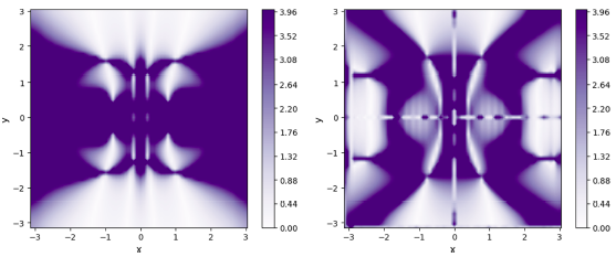
Figure 14. Ratio of the absolute values of the double derivatives $( r = (({\partial _x^2})/({\partial _y^2})))$
of
$( r = (({\partial _x^2})/({\partial _y^2})))$
of $b_x$
(left plot) and
$b_x$
(left plot) and $b_y$
(right plot), clipped at
$b_y$
(right plot), clipped at $r=4$
to avoid extreme dynamical range.
$r=4$
to avoid extreme dynamical range.
A.2. Details of the Eigenvalue Solver
The strategy is to express the linear operators, $\mathcal{M}$
and
$\mathcal{M}$
and $\mathcal{L}$
, as matrices acting on a state vector,
$\mathcal{L}$
, as matrices acting on a state vector, $v$
. Given these matrices, their eigenvalues, and the corresponding eigenvectors, can be found using publicly available schemes in many Python packages e.g. SciPy (Virtanen et al. Reference Virtanen2020), and PyTorch (Ansel et al. Reference Ansel2024).
$v$
. Given these matrices, their eigenvalues, and the corresponding eigenvectors, can be found using publicly available schemes in many Python packages e.g. SciPy (Virtanen et al. Reference Virtanen2020), and PyTorch (Ansel et al. Reference Ansel2024).
We choose a numerical grid with $N_x$
and
$N_x$
and $N_y$
collocation points in the
$N_y$
collocation points in the $x$
and the
$x$
and the $y$
directions, respectively. The eigenfunction now comprises
$y$
directions, respectively. The eigenfunction now comprises $N_x \times N_y$
values for each of
$N_x \times N_y$
values for each of $u_x$
,
$u_x$
, $u_y$
,
$u_y$
, $b_x$
and
$b_x$
and $b_y$
. We flatten this eigenfunction to get the state vector,
$b_y$
. We flatten this eigenfunction to get the state vector, $v$
, with
$v$
, with $4\times N_x \times N_y$
entries. The derivative operators are constructed by going to Fourier space, multiplying by appropriate powers of
$4\times N_x \times N_y$
entries. The derivative operators are constructed by going to Fourier space, multiplying by appropriate powers of $ik_x$
and
$ik_x$
and $ik_y$
, and taking the inverse Fourier transform.
$ik_y$
, and taking the inverse Fourier transform.
We then write a Python function with a dummy state vector as the argument which splits and reshapes it to give $u_x$
,
$u_x$
, $u_y$
,
$u_y$
, $b_x$
and
$b_x$
and $b_y$
over the 2-D grid, calculates the terms on the right-hand sides of equations (2.7)–(2.10), and give these as output after flattening it back to a
$b_y$
over the 2-D grid, calculates the terms on the right-hand sides of equations (2.7)–(2.10), and give these as output after flattening it back to a $4\times N_x \times N_y$
shape. The same is done for the left-hand sides of equations (2.7)–(2.10), without the
$4\times N_x \times N_y$
shape. The same is done for the left-hand sides of equations (2.7)–(2.10), without the $\gamma$
factor, which will be the eigenvalue obtained on solving the EVP. These functions take the state vector as the input and give as output a vector obtained by operating
$\gamma$
factor, which will be the eigenvalue obtained on solving the EVP. These functions take the state vector as the input and give as output a vector obtained by operating $\mathcal{M}$
and
$\mathcal{M}$
and $\mathcal{L}$
on the state vector. We now wish to obtain the matrix equivalent of these functions. This is done by first packaging the functions as scipy.sparse.linalg.LinearOperator objects, and then getting the matrix form of these objects by acting these on the identity matrix – thus giving us the matrix form of
$\mathcal{L}$
on the state vector. We now wish to obtain the matrix equivalent of these functions. This is done by first packaging the functions as scipy.sparse.linalg.LinearOperator objects, and then getting the matrix form of these objects by acting these on the identity matrix – thus giving us the matrix form of $\mathcal{M}$
and
$\mathcal{M}$
and $\mathcal{L}$
, each of size
$\mathcal{L}$
, each of size $4 N_x N_y \times 4 N_x N_y$
.
$4 N_x N_y \times 4 N_x N_y$
.
The eigenvalues and eigenvectors for these matrices can now be calculated using standard methods. In anticipation of large runtimes due to the large size of the matrices, we resort to using a GPU-based Python library – pytorch. We use the torch.linalg.eig package to get the eigenvalues and eigenvectors of the eigensystem comprising the $\mathcal{M}$
and
$\mathcal{M}$
and $\mathcal{L}$
matrices. The numerical implementation of this full procedure has been made public in a GitHub repository – SPEC-Tear.
$\mathcal{L}$
matrices. The numerical implementation of this full procedure has been made public in a GitHub repository – SPEC-Tear.
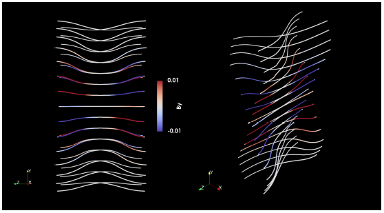
Figure 15. Magnetic field lines in the full 3-D case. The colors show the $y$
-component of the magnetic field.
$y$
-component of the magnetic field.
A.3. Low-pass filtering and periodicity of the equilibrium
We ensure periodicity of the equilibrium in the following way. The equilibrium is decomposed into its Fourier modes. Since the equilibrium is not strictly periodic, the Fourier coefficients for high wavenumbers are not zero, as would be the case for periodic functions. We now manually set the Fourier coefficients for wavenumbers above a chosen threshold to zero. The inverse Fourier transform of this gives us a perfectly periodic equilibrium. It is this process that we refer to as a low-pass filter – since it gets rid of high wavenumber (frequency) modes, ensuring periodicity of the equilibrium.
A.4. Magnetic island structure and null points
The structure of the magnetic islands and the array of magnetic null points for the full 3-D case is depicted by showing the magnetic field lines in figure 15. The colors indicate that $b_y$
is indeed non-zero, leading to a bent magnetic island structure. Note the symmetry of the structures across the
$b_y$
is indeed non-zero, leading to a bent magnetic island structure. Note the symmetry of the structures across the $y=0$
line. The most important aspect is that we recover 2-D-like X-point sites which allow the classic ‘cutting and rejoining’ type of reconnections to occur plane by plane. More sophisticated geometries of magnetic fields may not allow for such simple manifestation of magnetic nulls.
$y=0$
line. The most important aspect is that we recover 2-D-like X-point sites which allow the classic ‘cutting and rejoining’ type of reconnections to occur plane by plane. More sophisticated geometries of magnetic fields may not allow for such simple manifestation of magnetic nulls.


 Open access