


1 Introduction
Let K be a number field of degree n, and let $f \in \mathbb {Z}[t]$
be a polynomial. A central problem in arithmetic geometry is to determine under what conditions f can take values equal to a norm of an element of K. In order to address this question, we take an integral basis
$f \in \mathbb {Z}[t]$
be a polynomial. A central problem in arithmetic geometry is to determine under what conditions f can take values equal to a norm of an element of K. In order to address this question, we take an integral basis $\omega _1, \ldots , \omega _n$
for K, viewed as a vector space over
$\omega _1, \ldots , \omega _n$
for K, viewed as a vector space over $\mathbb {Q}$
, and define the norm form as
$\mathbb {Q}$
, and define the norm form as $\mathbf {N}(\mathbf {x}) = N_{K/\mathbb {Q}}(\omega _1x_1+ \cdots +\omega _nx_n)$
, where
$\mathbf {N}(\mathbf {x}) = N_{K/\mathbb {Q}}(\omega _1x_1+ \cdots +\omega _nx_n)$
, where $N_{K/\mathbb {Q}}(\cdot )$
is the field norm. We then seek to understand when the equation
$N_{K/\mathbb {Q}}(\cdot )$
is the field norm. We then seek to understand when the equation
 $$ \begin{align} f(t) = \mathbf{N}(\mathbf{x}) \neq 0 \end{align} $$
has a solution with $(t,x_1, \ldots , x_n) \in \mathbb {Q}^{n+1}$
. A necessary condition for solubility over
$(t,x_1, \ldots , x_n) \in \mathbb {Q}^{n+1}$
. A necessary condition for solubility over $\mathbb {Q}$
is that (1.1) must have solutions in
$\mathbb {Q}$
is that (1.1) must have solutions in $\mathbb {R}^{n+1}$
and in
$\mathbb {R}^{n+1}$
and in $\mathbb {Q}_p^{n+1}$
for every prime p. We say that the Hasse principle holds if this condition alone is sufficient to guarantee existence of a solution to (1.1) over
$\mathbb {Q}_p^{n+1}$
for every prime p. We say that the Hasse principle holds if this condition alone is sufficient to guarantee existence of a solution to (1.1) over $\mathbb {Q}$
.
$\mathbb {Q}$
.
Local to global questions for (1.1) have received much attention over the years. The first case to consider is when f is a nonzero constant polynomial. Here, the Hasse principle for (1.1) is known as the Hasse norm principle. More precisely, we say that the Hasse norm principle holds for the extension $K/\mathbb {Q}$
if
$K/\mathbb {Q}$
if $\mathbb {Q}^{\times }\cap N_{K/\mathbb {Q}}(I_K) = N_{K/\mathbb {Q}}(K^{\times })$
, where
$\mathbb {Q}^{\times }\cap N_{K/\mathbb {Q}}(I_K) = N_{K/\mathbb {Q}}(K^{\times })$
, where $I_K = \mathbb {A}_K^{\times }$
is the group of ideles of K. The Hasse norm principle has been extensively studied, beginning with the work of Hasse himself, who established that it holds for cyclic extensions
$I_K = \mathbb {A}_K^{\times }$
is the group of ideles of K. The Hasse norm principle has been extensively studied, beginning with the work of Hasse himself, who established that it holds for cyclic extensions $K/\mathbb {Q}$
(a result known as the Hasse norm theorem), but does not hold for certain biquadratic extensions, such as
$K/\mathbb {Q}$
(a result known as the Hasse norm theorem), but does not hold for certain biquadratic extensions, such as $K = \mathbb {Q}(\sqrt {13},\sqrt {-3})$
. The Hasse norm principle is also known to hold if the degree of K is prime (Bartels [Reference Bartels1]) or if the normal closure of K has Galois group
$K = \mathbb {Q}(\sqrt {13},\sqrt {-3})$
. The Hasse norm principle is also known to hold if the degree of K is prime (Bartels [Reference Bartels1]) or if the normal closure of K has Galois group $S_n$
(Kunyavskiı̆ and Voskresenskiı̆ [32]) or
$S_n$
(Kunyavskiı̆ and Voskresenskiı̆ [32]) or $A_n$
for
$A_n$
for $n \neq 4$
(Macedo [Reference Macedo35]).
$n \neq 4$
(Macedo [Reference Macedo35]).
When $[K:\mathbb {Q}]=2$
and f is irreducible of degree
$[K:\mathbb {Q}]=2$
and f is irreducible of degree $3$
or
$3$
or $4$
, (1.1) defines a Châtelet surface. There are now many known counterexamples to the Hasse principle for Châtelet surfaces, including one by Iskovskikh [Reference Iskovskikh28], which we discuss in more detail in Example 5.4. However, Colliot-Thélène, Sansuc and Swinnerton-Dyer [Reference Colliot-Thélène, Sansuc and Swinnerton-Dyer14] prove that the Brauer–Manin obstruction accounts for all failures of the Hasse principle. A similar result holds when f is an irreducible polynomial of degree at most
$4$
, (1.1) defines a Châtelet surface. There are now many known counterexamples to the Hasse principle for Châtelet surfaces, including one by Iskovskikh [Reference Iskovskikh28], which we discuss in more detail in Example 5.4. However, Colliot-Thélène, Sansuc and Swinnerton-Dyer [Reference Colliot-Thélène, Sansuc and Swinnerton-Dyer14] prove that the Brauer–Manin obstruction accounts for all failures of the Hasse principle. A similar result holds when f is an irreducible polynomial of degree at most $3$
and
$3$
and $[K:\mathbb {Q}]=3$
, as proved by Colliot-Thélène and Salberger [Reference Colliot-Thélène and Salberger8]. Both of these results make use of fibration and descent methods.
$[K:\mathbb {Q}]=3$
, as proved by Colliot-Thélène and Salberger [Reference Colliot-Thélène and Salberger8]. Both of these results make use of fibration and descent methods.
In the case when f is an irreducible quadratic and K is a quartic extension containing a root of f, the Hasse principle and weak approximation are known to hold for (1.1) thanks to the work of Browning and Heath-Brown [Reference Browning and Heath-Brown4]. This result was generalised by Derenthal, Smeets and Wei [Reference Derenthal, Smeets and Wei16, Theorem 2] to prove that the Brauer–Manin obstruction is the only obstruction to the Hasse principle and weak approximation for irreducible quadratics f and arbitrary number fields K. Moreover, in [Reference Derenthal, Smeets and Wei16, Theorem 4], they give an explicit description of the Brauer groups that can be obtained in this family.
Results when f is not irreducible have so far been limited to products of linear polynomials. Suppose that f takes the form
 $$ \begin{align} f(t) = c\prod_{i=1}^r (t-e_i)^{m_i}, \end{align} $$
for some $c\in \mathbb {Q}^*, e_1, \ldots , e_r \in \mathbb {Q}$
and
$c\in \mathbb {Q}^*, e_1, \ldots , e_r \in \mathbb {Q}$
and $m_1, \ldots , m_r \in \mathbb {N}$
. When
$m_1, \ldots , m_r \in \mathbb {N}$
. When $r=1$
, the Brauer–Manin obstruction is the only obstruction to the Hasse principle and weak approximation for any smooth projective model of (1.1). This is a special case of the work of Colliot-Thélène and Sansuc [Reference Colliot-Thélène and Sansuc9] on principal homogeneous spaces under algebraic tori. Heath-Brown and Skorobogatov [Reference Heath-Brown and Skorobogatov26] treat the case
$r=1$
, the Brauer–Manin obstruction is the only obstruction to the Hasse principle and weak approximation for any smooth projective model of (1.1). This is a special case of the work of Colliot-Thélène and Sansuc [Reference Colliot-Thélène and Sansuc9] on principal homogeneous spaces under algebraic tori. Heath-Brown and Skorobogatov [Reference Heath-Brown and Skorobogatov26] treat the case $r=2$
by combining descent methods with the Hardy–Littlewood circle method, under the assumption that
$r=2$
by combining descent methods with the Hardy–Littlewood circle method, under the assumption that $\gcd (m_1,m_2,\deg K)=1$
. This assumption was later removed by Colliot-Thélène, Harari and Skorobogatov [Reference Colliot-Thélène, Harari and Skorobogatov13]. Thanks to the work of Browning and Matthiesen [Reference Browning and Matthiesen5], it is now settled that for any number field K and polynomial f of the form (1.2) (for arbitrary
$\gcd (m_1,m_2,\deg K)=1$
. This assumption was later removed by Colliot-Thélène, Harari and Skorobogatov [Reference Colliot-Thélène, Harari and Skorobogatov13]. Thanks to the work of Browning and Matthiesen [Reference Browning and Matthiesen5], it is now settled that for any number field K and polynomial f of the form (1.2) (for arbitrary $r \geqslant 1$
), the Brauer–Manin obstruction is the only obstruction to the Hasse principle and weak approximation for any smooth projective model of (1.1). Their result is inspired by additive combinatorics results of Green, Tao and Ziegler [Reference Green and Tao20], [Reference Green, Tao and Ziegler21], combined with vertical torsors introduced by Schindler and Skorobogatov [Reference Schindler and Skorobogatov40].
$r \geqslant 1$
), the Brauer–Manin obstruction is the only obstruction to the Hasse principle and weak approximation for any smooth projective model of (1.1). Their result is inspired by additive combinatorics results of Green, Tao and Ziegler [Reference Green and Tao20], [Reference Green, Tao and Ziegler21], combined with vertical torsors introduced by Schindler and Skorobogatov [Reference Schindler and Skorobogatov40].
In general, it has been conjectured by Colliot-Thélène [Reference Colliot-Thélène7] that all failures of the Hasse principle for any smooth projective model of (1.1) are explained by the Brauer–Manin obstruction. Assuming Schinzel’s hypothesis, this holds true for f an arbitrary polynomial and $K/\mathbb {Q}$
a cyclic extension, as demonstrated by work of Colliot-Thélène and Swinnerton-Dyer on pencils of Severi–Brauer varieties [Reference Colliot-Thélène and Swinnerton-Dyer12]. Recently, Skorobogatov and Sofos also establish unconditionally that when
$K/\mathbb {Q}$
a cyclic extension, as demonstrated by work of Colliot-Thélène and Swinnerton-Dyer on pencils of Severi–Brauer varieties [Reference Colliot-Thélène and Swinnerton-Dyer12]. Recently, Skorobogatov and Sofos also establish unconditionally that when $K/\mathbb {Q}$
is cyclic, (1.1) satisfies the Hasse principle for a positive proportion of polynomials f of degree d, when their coefficients are ordered by height [Reference Skorobogatov and Sofos42, Theorem 1.3].
$K/\mathbb {Q}$
is cyclic, (1.1) satisfies the Hasse principle for a positive proportion of polynomials f of degree d, when their coefficients are ordered by height [Reference Skorobogatov and Sofos42, Theorem 1.3].
In [Reference Irving27], Irving introduces an entirely new approach to studying the Hasse principle for (1.1), which rests on sieve methods. Irving’s main result [Reference Irving27, Theorem 1.1] states that if $f\in \mathbb {Z}[t]$
is an irreducible cubic, then the Hasse principle holds for (1.1) under the following assumptions:
$f\in \mathbb {Z}[t]$
is an irreducible cubic, then the Hasse principle holds for (1.1) under the following assumptions:
-
(1) K satisfies the Hasse norm principle.
-
(2) There exists a prime $q\geqslant 7$
and a finite set of primes S, such that for all
$p\notin S$
, either
$p\equiv 1 \ (\mathrm {mod}\ q)$
or the inertia degrees of p in
$K/\mathbb {Q}$
are coprime.
$q\geqslant 7$
and a finite set of primes S, such that for all
$p\notin S$
, either
$p\equiv 1 \ (\mathrm {mod}\ q)$
or the inertia degrees of p in
$K/\mathbb {Q}$
are coprime. -
(3) The number field generated by f is not contained in the cyclotomic field
$\mathbb {Q}(\zeta _q)$
.


An example provided by Irving in [Reference Irving27] is the number field $\mathbb {Q}(\alpha )$
, where
$\mathbb {Q}(\alpha )$
, where $\alpha $
is a root of
$\alpha $
is a root of $x^q-2$
and
$x^q-2$
and $q \geqslant 7$
is prime. We shall comment on this further in Example 5.9.
$q \geqslant 7$
is prime. We shall comment on this further in Example 5.9.
In this paper, we generalize Irving’s arguments to establish the Hasse principle for a wide new family of polynomials and number fields. Our results cover for the first time polynomials of arbitrarily large degree which are not a product of linear factors. In fact, under suitable assumptions on K, we can deal with polynomials that are products of arbitrarily many linear, quadratic and cubic factors.
Throughout this paper, we let $\widehat {K}$
denote the Galois closure of K, and we let
$\widehat {K}$
denote the Galois closure of K, and we let $G = \mathrm {Gal}(\widehat {K}/\mathbb {Q})$
, viewed as a permutation group on n letters. We define
$G = \mathrm {Gal}(\widehat {K}/\mathbb {Q})$
, viewed as a permutation group on n letters. We define
 $$ \begin{align} T(G) = \frac{1}{\#G}\#\{\sigma \in G: \textrm{ the cycle lengths of }\sigma\textrm{ are not coprime}\}. \end{align} $$
We now state our main results.
Theorem 1.1. Let K be a number field satisfying the Hasse norm principle. Let $f\in \mathbb {Z}[t]$
be a polynomial, all of whose irreducible factors have degree at most 2. Let k denote the number of distinct irreducible factors of f, and let j denote the number of distinct irreducible quadratic factors of f which generate a quadratic field contained in
$f\in \mathbb {Z}[t]$
be a polynomial, all of whose irreducible factors have degree at most 2. Let k denote the number of distinct irreducible factors of f, and let j denote the number of distinct irreducible quadratic factors of f which generate a quadratic field contained in $\widehat {K}$
. Suppose that
$\widehat {K}$
. Suppose that $T(G) \leqslant \frac {0.39}{k+j+1}$
. Then the Hasse principle holds for (1.1).
$T(G) \leqslant \frac {0.39}{k+j+1}$
. Then the Hasse principle holds for (1.1).
In practice, the constant $0.39$
can be improved slightly, particularly when the majority of the factors of f are linear, although it will always be less than
$0.39$
can be improved slightly, particularly when the majority of the factors of f are linear, although it will always be less than $1/2$
. The precise optimal constant is obtained by finding the maximal value of
$1/2$
. The precise optimal constant is obtained by finding the maximal value of $\kappa $
such that (4.55) holds.
$\kappa $
such that (4.55) holds.
When $G=S_n$
, we shall see in Lemma 5.10 that
$G=S_n$
, we shall see in Lemma 5.10 that $T(S_n) \rightarrow 0$
as
$T(S_n) \rightarrow 0$
as $n \rightarrow \infty $
, so in the setting of Theorem 1.1, we can establish the Hasse principle provided n is sufficiently large in terms of the degree of f. We illustrate this by treating the case when f is a product of two irreducible quadratics.
$n \rightarrow \infty $
, so in the setting of Theorem 1.1, we can establish the Hasse principle provided n is sufficiently large in terms of the degree of f. We illustrate this by treating the case when f is a product of two irreducible quadratics.
Corollary 1.2. Let $f \in \mathbb {Z}[t]$
be a product of two quadratic polynomials such that the number field L generated by f is a biquadratic extension of
$f \in \mathbb {Z}[t]$
be a product of two quadratic polynomials such that the number field L generated by f is a biquadratic extension of $\mathbb {Q}$
. Let K be a number field of degree n with
$\mathbb {Q}$
. Let K be a number field of degree n with $G=S_n$
. Suppose that
$G=S_n$
. Suppose that $L\cap \widehat {K} = \mathbb {Q}$
. Then the Hasse principle holds for (1.1), provided that
$L\cap \widehat {K} = \mathbb {Q}$
. Then the Hasse principle holds for (1.1), provided that
 $$ \begin{align*}n\not\in\{2,3,\ldots, 10, 12,14,15,16,18,20,22,24,26,28,30,36,42,48\}.\end{align*} $$
We remark that without the assumption $L\cap \widehat {K} = \mathbb {Q}$
, a similar result to Corollary 1.2 still holds, although a larger list of degrees n would need to be excluded. For example, if
$L\cap \widehat {K} = \mathbb {Q}$
, a similar result to Corollary 1.2 still holds, although a larger list of degrees n would need to be excluded. For example, if $L\cap \widehat {K}$
is quadratic, then the Hasse principle holds for (1.1) for all primes
$L\cap \widehat {K}$
is quadratic, then the Hasse principle holds for (1.1) for all primes $n\geqslant 11$
and all integers
$n\geqslant 11$
and all integers $n>90$
, whilst if
$n>90$
, whilst if $L\cap \widehat {K} = L$
, then the Hasse prinicple holds for all primes
$L\cap \widehat {K} = L$
, then the Hasse prinicple holds for all primes $n\geqslant 13$
and all integers
$n\geqslant 13$
and all integers $n>150$
.
$n>150$
.
We cannot hope to deal with all small values of n in Corollary 1.2. For example, the work of Iskovskikh [Reference Iskovskikh28] shows that the Hasse principle can fail when $n=2$
(see Example 5.4). However, as we shall discuss in Appendix A, in the case
$n=2$
(see Example 5.4). However, as we shall discuss in Appendix A, in the case $n\geqslant 3$
, there is no Brauer–Manin obstruction to the Hasse principle, and so according to the conjecture of Colliot-Thélène mentioned above, we should expect the Hasse principle to hold.
$n\geqslant 3$
, there is no Brauer–Manin obstruction to the Hasse principle, and so according to the conjecture of Colliot-Thélène mentioned above, we should expect the Hasse principle to hold.
Our second main result allows f to contain irreducible cubic factors but requires more restrictive assumptions on the number field K, more similar to Irving’s setup in [Reference Irving27].
Theorem 1.3. Let $f\in \mathbb {Z}[t]$
be a polynomial, all of whose irreducible factors have degree at most
$f\in \mathbb {Z}[t]$
be a polynomial, all of whose irreducible factors have degree at most $3$
. Then the Hasse principle holds for (1.1) under the following assumptions for K.
$3$
. Then the Hasse principle holds for (1.1) under the following assumptions for K.
-
(1) K satisfies the Hasse norm principle.
-
(2) The set
$\mathcal {P}$
of primes p for which the inertia degrees of p in
$K/\mathbb {Q}$
are not coprime satisfies Assumption 2.2.


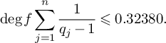
As an example, Assumption 2.2 is satisfied if there exists a prime q such that $\frac {\deg f +1}{q-1}\leqslant 0.32380$
, and such that for all but finitely many primes
$\frac {\deg f +1}{q-1}\leqslant 0.32380$
, and such that for all but finitely many primes $p\not \equiv 1 \ (\mathrm {mod}\ q)$
, the inertia degrees of p in
$p\not \equiv 1 \ (\mathrm {mod}\ q)$
, the inertia degrees of p in $K/\mathbb {Q}$
are coprime. The constant
$K/\mathbb {Q}$
are coprime. The constant $0.32380$
appearing in Assumption 2.2 could likely be improved with more work, and in specific examples, the required bounds could be computed more precisely using (4.59). We remark that we have also dropped the assumption made in [Reference Irving27] that the number field generated by f is not contained in
$0.32380$
appearing in Assumption 2.2 could likely be improved with more work, and in specific examples, the required bounds could be computed more precisely using (4.59). We remark that we have also dropped the assumption made in [Reference Irving27] that the number field generated by f is not contained in $\mathbb {Q}(\zeta _q)$
. This assumption is not essential to Irving’s argument, but allows for the treatment of smaller values of q. Reinserting this assumption and optimising (4.59), we could recover Irving’s result from our work.
$\mathbb {Q}(\zeta _q)$
. This assumption is not essential to Irving’s argument, but allows for the treatment of smaller values of q. Reinserting this assumption and optimising (4.59), we could recover Irving’s result from our work.
We prove Theorems 1.1 and 1.3 by applying the beta sieve of Rosser and Iwaniec [Reference Friedlander and Iwaniec18, Theorem 11.13]. The main sieve results we obtain are stated in Theorems 2.1 and 2.3. These results in fact prove the existence of a solution to (1.1) with t arbitrarily close to a given adelic solution. Consequently, the above results could be extended to prove weak approximation for (1.1), provided that weak approximation holds for the norm one torus $\mathbf {N}(\mathbf {x})=1$
. For example, the work of Kunyavskiı̆ and Voskresenskiı̆ [32] and Macedo [Reference Macedo35] demonstrates that weak approximation for the norm one torus holds when
$\mathbf {N}(\mathbf {x})=1$
. For example, the work of Kunyavskiı̆ and Voskresenskiı̆ [32] and Macedo [Reference Macedo35] demonstrates that weak approximation for the norm one torus holds when $G=S_n$
or
$G=S_n$
or $G=A_n$
and
$G=A_n$
and $n \neq 4$
, and so weak approximation holds in the setting of Corollary 1.2.
$n \neq 4$
, and so weak approximation holds in the setting of Corollary 1.2.
In Section 6, we find a second application of Theorem 2.1 to a conjecture of Harpaz and Wittenberg [Reference Harpaz and Wittenberg23, Conjecture 9.1], which we restate in Conjecture 6.1 and henceforth refer to as the Harpaz–Wittenberg conjecture. The conjecture concerns a collection of number field extensions $L_i/k_i/k$
,
$L_i/k_i/k$
, $i\in \{1, \ldots , n\}$
, where
$i\in \{1, \ldots , n\}$
, where $k_i \cong k[t]/(P_i(t))$
for monic irreducible polynomials
$k_i \cong k[t]/(P_i(t))$
for monic irreducible polynomials $P_i \in k[t]$
. Roughly speaking, the conjecture predicts, under certain hypotheses, the existence of an element
$P_i \in k[t]$
. Roughly speaking, the conjecture predicts, under certain hypotheses, the existence of an element $t_0\in k$
such that
$t_0\in k$
such that $P_1(t_0), \ldots ,P_n(t_0)$
are locally split (i.e., each place in
$P_1(t_0), \ldots ,P_n(t_0)$
are locally split (i.e., each place in $k_i$
dividing
$k_i$
dividing $P_i(t_0)$
has a degree
$P_i(t_0)$
has a degree $1$
place of
$1$
place of $L_i$
above it).
$L_i$
above it).
A major motivation for the conjecture is the development of the theory of rational points in fibrations. Given a fibration $\pi :X\rightarrow \mathbb {P}^1_{k}$
, a natural question is to what extent we can deduce arithmetic information about X from arithmetic information about the fibres of
$\pi :X\rightarrow \mathbb {P}^1_{k}$
, a natural question is to what extent we can deduce arithmetic information about X from arithmetic information about the fibres of $\pi $
. A famous conjecture of Colliot-Thélène [Reference Colliot-Thélène7, p.174] predicts that for any smooth, proper, geometrically irreducible, rationally connected variety X over a number field k, the rational points
$\pi $
. A famous conjecture of Colliot-Thélène [Reference Colliot-Thélène7, p.174] predicts that for any smooth, proper, geometrically irreducible, rationally connected variety X over a number field k, the rational points $X(k)$
are dense in the Brauer–Manin set
$X(k)$
are dense in the Brauer–Manin set $X(\mathbb {A}_k)^{\operatorname {Br}}$
. (In other words, the Brauer–Manin obstruction is the only obstruction to weak approximation.) Applied to this conjecture, the above question becomes whether density of
$X(\mathbb {A}_k)^{\operatorname {Br}}$
. (In other words, the Brauer–Manin obstruction is the only obstruction to weak approximation.) Applied to this conjecture, the above question becomes whether density of $X(k)$
in
$X(k)$
in $X(\mathbb {A}_k)^{\operatorname {Br}}$
follows from density of
$X(\mathbb {A}_k)^{\operatorname {Br}}$
follows from density of $X_c(k)$
in
$X_c(k)$
in $X_c(\mathbb {A}_k)^{\operatorname {Br}}$
for a general fibre
$X_c(\mathbb {A}_k)^{\operatorname {Br}}$
for a general fibre ![]() of
of $\pi $
(see [Reference Harpaz, Wei and Wittenberg24, Question 1.2]). Applications of the Harpaz–Wittenberg conjecture to this question are studied in [Reference Harpaz and Wittenberg23] and [Reference Harpaz, Wei and Wittenberg24].
$\pi $
(see [Reference Harpaz, Wei and Wittenberg24, Question 1.2]). Applications of the Harpaz–Wittenberg conjecture to this question are studied in [Reference Harpaz and Wittenberg23] and [Reference Harpaz, Wei and Wittenberg24].
Harpaz and Wittenberg [Reference Harpaz and Wittenberg23, Section 9.2] demonstrate that their conjecture follows from the homogeneous version of Schinzel’s hypothesis (commonly reffered to as $(\textrm {HH}_1)$
) in the case of abelian extensions
$(\textrm {HH}_1)$
) in the case of abelian extensions $L_i/k_i$
, or more generally, almost abelian extensions (see [Reference Harpaz and Wittenberg23, Definition 9.4]). Examples of almost abelian extensions include cubic extensions, and extensions of the form
$L_i/k_i$
, or more generally, almost abelian extensions (see [Reference Harpaz and Wittenberg23, Definition 9.4]). Examples of almost abelian extensions include cubic extensions, and extensions of the form $k(c^{1/p})/k$
for
$k(c^{1/p})/k$
for $c\in k$
and p prime. The work of Heath-Brown and Moroz [Reference Heath-Brown and Moroz25] establishes
$c\in k$
and p prime. The work of Heath-Brown and Moroz [Reference Heath-Brown and Moroz25] establishes $(\textrm {HH}_1)$
for primes represented by binary cubic forms, from which the Harpaz–Wittenberg conjecture can be deduced in the case
$(\textrm {HH}_1)$
for primes represented by binary cubic forms, from which the Harpaz–Wittenberg conjecture can be deduced in the case $k=\mathbb {Q}, n=1$
and
$k=\mathbb {Q}, n=1$
and $\deg P_1 = 3$
. Using a geometric reformulation of [Reference Harpaz and Wittenberg23, Conjecture 9.1], the authors establish their conjecture in low-degree cases – namely, when
$\deg P_1 = 3$
. Using a geometric reformulation of [Reference Harpaz and Wittenberg23, Conjecture 9.1], the authors establish their conjecture in low-degree cases – namely, when $\sum _{i=1}^n [k_i:k] \leqslant 2$
or
$\sum _{i=1}^n [k_i:k] \leqslant 2$
or $\sum _{i=1}^n [k_i:k]=3$
and
$\sum _{i=1}^n [k_i:k]=3$
and $[L_i:k_i]=2$
for all i.
$[L_i:k_i]=2$
for all i.
The Harpaz–Wittenberg conjecture is related to the study of polynomials represented by norm forms. As a consequence of the work of Matthiesen [Reference Matthiesen36] on norms as products of linear polynomials, the Harpaz–Wittenberg conjecture holds in the case $k_1=\cdots = k_n = k =\mathbb {Q}$
[Reference Harpaz and Wittenberg23, Theorem 9.14]. Similarly, we can deduce from [Reference Irving27, Theorem 1.1] that the Harpaz–Wittenberg conjecture holds in the case
$k_1=\cdots = k_n = k =\mathbb {Q}$
[Reference Harpaz and Wittenberg23, Theorem 9.14]. Similarly, we can deduce from [Reference Irving27, Theorem 1.1] that the Harpaz–Wittenberg conjecture holds in the case $n=2, k=\mathbb {Q}, k_1=K,k_2=\mathbb {Q}, L_1 = K(2^{1/q})$
and
$n=2, k=\mathbb {Q}, k_1=K,k_2=\mathbb {Q}, L_1 = K(2^{1/q})$
and $L_2 = \mathbb {Q}(2^{1/q})$
, where
$L_2 = \mathbb {Q}(2^{1/q})$
, where $q\geqslant 7$
is a prime such that
$q\geqslant 7$
is a prime such that $K\not \subseteq \mathbb {Q}(\zeta _q)$
[Reference Harpaz and Wittenberg23, Theorem 9.15].
$K\not \subseteq \mathbb {Q}(\zeta _q)$
[Reference Harpaz and Wittenberg23, Theorem 9.15].
Besides the work of Matthiesen [Reference Matthiesen36] for $k_1 = \cdots = k_n = k = \mathbb {Q}$
, the aforementioned results apply only to the case
$k_1 = \cdots = k_n = k = \mathbb {Q}$
, the aforementioned results apply only to the case $n\leqslant 2$
. In Section 6, we prove the following theorem, which establishes the Harpaz–Wittenberg conjecture in a new family of extensions
$n\leqslant 2$
. In Section 6, we prove the following theorem, which establishes the Harpaz–Wittenberg conjecture in a new family of extensions $k_1/\mathbb {Q}, \ldots , k_n/\mathbb {Q}$
, where n may be arbitrarily large, and each extension
$k_1/\mathbb {Q}, \ldots , k_n/\mathbb {Q}$
, where n may be arbitrarily large, and each extension $k_i/\mathbb {Q}$
may have degree up to
$k_i/\mathbb {Q}$
may have degree up to $3$
.
$3$
.
Theorem 1.4. Let $n\geqslant 1$
. Let
$n\geqslant 1$
. Let $k=\mathbb {Q}$
, and for
$k=\mathbb {Q}$
, and for $i\in \{1, \ldots , n\}$
, let
$i\in \{1, \ldots , n\}$
, let $k_i, M_i$
be linearly disjoint number fields over
$k_i, M_i$
be linearly disjoint number fields over $\mathbb {Q}$
. Let
$\mathbb {Q}$
. Let $L_i = M_ik_i$
be the compositum of
$L_i = M_ik_i$
be the compositum of $k_i$
and
$k_i$
and $M_i$
. Define
$M_i$
. Define
 $$ \begin{align}T_i = \frac{1}{\#\mathrm{Gal}(\widehat{M_i}/\mathbb{Q})}\#\{\sigma \in \mathrm{Gal}(\widehat{M}_i/\mathbb{Q}): \sigma \textrm{ has no fixed point}\}. \end{align} $$
Let $d = \sum _{i=1}^n [k_i:\mathbb {Q}]$
. Then the Harpaz–Wittenberg conjecture holds in the following cases.
$d = \sum _{i=1}^n [k_i:\mathbb {Q}]$
. Then the Harpaz–Wittenberg conjecture holds in the following cases.
-
(1)
$[k_i:\mathbb {Q}]\leqslant 2$
for all
$i\in \{1, \ldots , n\}$
and
$\sum _{i=1}^n T_i \leqslant 0.39/d$
. -
(2)
$[k_i:\mathbb {Q}]\leqslant 3$
for all
$i\in \{1, \ldots , n\}$
, and there exist primes
$q_i$
satisfying
$\sum _{i=1}^n 1/(q_i-1)\leqslant 0.32380/d$
, and integers
$t_i$
coprime to
$q_i$
, such that for all but finitely many primes
$p \not \equiv t_i\ (\mathrm {mod}\ q_i)$
, there is a place of degree
$1$
in
$M_i$
above p.


Corollary 1.5. Let $q_1, \ldots , q_n$
be distinct primes, and let
$q_1, \ldots , q_n$
be distinct primes, and let $r_1, \ldots , r_n \in \mathbb {N}$
be such that
$r_1, \ldots , r_n \in \mathbb {N}$
be such that $g_i(x) = x^{q_i}-r_i$
is irreducible for all i. Let
$g_i(x) = x^{q_i}-r_i$
is irreducible for all i. Let $M_i = \mathbb {Q}[x]/(g_i)$
and let
$M_i = \mathbb {Q}[x]/(g_i)$
and let $k_i,L_i$
and d be as in Theorem 1.4. Suppose that one of the following holds:
$k_i,L_i$
and d be as in Theorem 1.4. Suppose that one of the following holds:
-
(1)
$[k_i:\mathbb {Q}] \leqslant 2$
for all
$i\in \{1, \ldots , n\}$
and
$\sum _{i=1}^n 1/q_i \leqslant 0.39/d$
, -
(2)
$[k_i:\mathbb {Q}] \leqslant 3$
for all
$i \in \{1,\ldots ,n\}$
and
$\sum _{i=1}^n 1/(q_i-1) \leqslant 0.32380/d$
.


Then the Harpaz–Wittenberg conjecture holds for $k=\mathbb {Q}$
and for such choices of
$k=\mathbb {Q}$
and for such choices of $k_i$
and
$k_i$
and $L_i$
.
$L_i$
.
We remark that when applied to the setting of [Reference Harpaz and Wittenberg23, Theorem 9.15], the above result requires a stronger bound on q. However, with a more careful optimisation of (4.58), it should be possible to recover [Reference Harpaz and Wittenberg23, Theorem 9.15] from our approach.
By combining Theorem 1.4 with [Reference Harpaz and Wittenberg23, Theorem 9.17] (with the choice $B=0, M" = \emptyset $
and
$B=0, M" = \emptyset $
and $M' = \mathbb {P}^1_k\backslash U$
), we obtain the following result about rational points in fibrations.
$M' = \mathbb {P}^1_k\backslash U$
), we obtain the following result about rational points in fibrations.
Theorem 1.6. Let X be a smooth, proper, geometrically irreducible variety over $\mathbb {Q}$
. Let
$\mathbb {Q}$
. Let $\pi :X \rightarrow \mathbb {P}^1_{\mathbb {Q}}$
be a dominant morphism whose general fibre is rationally connected. Let
$\pi :X \rightarrow \mathbb {P}^1_{\mathbb {Q}}$
be a dominant morphism whose general fibre is rationally connected. Let $k_1, \ldots , k_n$
denote the residue fields of the closed points of
$k_1, \ldots , k_n$
denote the residue fields of the closed points of $\mathbb {P}^1_{\mathbb {Q}}$
above which
$\mathbb {P}^1_{\mathbb {Q}}$
above which $\pi $
has nonsplit fibres, and let
$\pi $
has nonsplit fibres, and let $L_i/k_i$
be finite extensions which split these nonsplit fibres. Assume that
$L_i/k_i$
be finite extensions which split these nonsplit fibres. Assume that
-
(1) The smooth fibres of
$\pi $
satisfy the Hasse principle and weak approximation. -
(2) The hypotheses of Theorem 1.4 hold.

Then $X(\mathbb {Q})$
is dense in
$X(\mathbb {Q})$
is dense in $X(\mathbb {A}_{\mathbb {Q}})^{\operatorname {\mathrm {Br}}(X)}$
.
$X(\mathbb {A}_{\mathbb {Q}})^{\operatorname {\mathrm {Br}}(X)}$
.
It would be interesting to investigate whether Condition $(1)$
in Theorem 1.6 could be relaxed to the assumption that the smooth fibres
$(1)$
in Theorem 1.6 could be relaxed to the assumption that the smooth fibres $X_c(\mathbb {Q})$
are dense in
$X_c(\mathbb {Q})$
are dense in $X_c(\mathbb {A}_{\mathbb {Q}})^{\operatorname {\mathrm {Br}}(X_c)}$
, as in the setting of [Reference Harpaz, Wei and Wittenberg24, Question 1.2] discussed above. This would require an extension of Theorem 1.4 to cover a stronger version of the Harpaz–Wittenberg conjecture, involving strong approximation of an auxiliary variety W off a finite set of places [Reference Harpaz, Wei and Wittenberg24, Proposition 6.1]. Strong approximation of W was studied by Browning and Schindler [Reference Browning and Schindler6], for example, who established [Reference Harpaz, Wei and Wittenberg24, Question 1.2] in the case when the rank of
$X_c(\mathbb {A}_{\mathbb {Q}})^{\operatorname {\mathrm {Br}}(X_c)}$
, as in the setting of [Reference Harpaz, Wei and Wittenberg24, Question 1.2] discussed above. This would require an extension of Theorem 1.4 to cover a stronger version of the Harpaz–Wittenberg conjecture, involving strong approximation of an auxiliary variety W off a finite set of places [Reference Harpaz, Wei and Wittenberg24, Proposition 6.1]. Strong approximation of W was studied by Browning and Schindler [Reference Browning and Schindler6], for example, who established [Reference Harpaz, Wei and Wittenberg24, Question 1.2] in the case when the rank of $\pi $
is at most
$\pi $
is at most $3$
, and at least one of its nonsplit fibres lies above a rational of
$3$
, and at least one of its nonsplit fibres lies above a rational of $\mathbb {P}^1_{\mathbb {Q}}$
.
$\mathbb {P}^1_{\mathbb {Q}}$
.
2 Main sieve results for binary forms
Let $f \in \mathbb {Z}[x,y]$
be a non-constant binary form with nonzero discriminant. We write
$f \in \mathbb {Z}[x,y]$
be a non-constant binary form with nonzero discriminant. We write $f(x,y)$
as a product of distinct irreducible factors
$f(x,y)$
as a product of distinct irreducible factors
 $$ \begin{align} f(x,y) = \prod_{i=0}^m f_i(x,y)\prod_{i=m+1}^k f_i(x,y), \end{align} $$
where $f_i(x,y)$
are linear forms for
$f_i(x,y)$
are linear forms for $1\leqslant i\leqslant m$
, and forms of degree
$1\leqslant i\leqslant m$
, and forms of degree $k_i\geqslant 2$
for
$k_i\geqslant 2$
for $m+1\leqslant i \leqslant k$
. If
$m+1\leqslant i \leqslant k$
. If $y\mid f(x,y)$
, then we define
$y\mid f(x,y)$
, then we define $f_0(x,y)=y$
, and otherwise, we let
$f_0(x,y)=y$
, and otherwise, we let $f_0(x,y)=1$
. Hence, we have
$f_0(x,y)=1$
. Hence, we have $y\nmid f_i(x,y)$
for all
$y\nmid f_i(x,y)$
for all $i\geqslant 1$
.
$i\geqslant 1$
.
For $i\in \{0,\ldots , k\}$
, we define
$i\in \{0,\ldots , k\}$
, we define
 $$ \begin{align} \nu_i(p) &= \#\{[x:y]\in \mathbb{P}^1(\mathbb{F}_p): f_i(x,y) \equiv 0 \ (\mathrm{mod}\ p)\}, \end{align} $$
 $$ \begin{align} \nu(p) &=\#\{[x:y]\in \mathbb{P}^1(\mathbb{F}_p): f(x,y) \equiv 0 \ (\mathrm{mod}\ p)\}. \end{align} $$
Let $\mathcal {P}$
be a set of primes, and let
$\mathcal {P}$
be a set of primes, and let $\mathcal {P}_{\leqslant x} = \{p\in \mathcal {P}:p\leqslant x\}$
. We denote by
$\mathcal {P}_{\leqslant x} = \{p\in \mathcal {P}:p\leqslant x\}$
. We denote by $\pi (x)$
the number of primes less than x. For all
$\pi (x)$
the number of primes less than x. For all $i\in \{0,\ldots , k\}$
, we need to assume
$i\in \{0,\ldots , k\}$
, we need to assume $\mathcal {P}$
has the following properties, for some
$\mathcal {P}$
has the following properties, for some $\alpha , \theta _i>0$
and any
$\alpha , \theta _i>0$
and any $A\geqslant 1$
:
$A\geqslant 1$
:
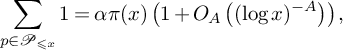 $$ \begin{align} \sum_{p \in \mathcal{P}_{\leqslant x}} 1 &= \alpha \pi(x)\left(1+O_A\left((\log x)^{-A}\right)\right), \end{align} $$
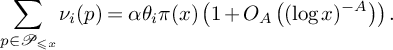 $$ \begin{align} \sum_{p \in \mathcal{P}_{\leqslant x}} \nu_i(p) &= \alpha\theta_i \pi(x)\left(1+O_A\left((\log x)^{-A}\right)\right). \end{align} $$
The reason we require explicit error terms in (2.4) and (2.5) is so that the sieve dimensions, introduced in Section 4.2, exist. We note that for $i=0$
, we have
$i=0$
, we have $\theta _0=1$
if
$\theta _0=1$
if $f_0(x,y) = y$
, and
$f_0(x,y) = y$
, and $\theta _0=0$
if
$\theta _0=0$
if $f_0(x,y)=1$
. Additionally, from (2.5), it follows that
$f_0(x,y)=1$
. Additionally, from (2.5), it follows that
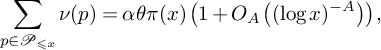 $$ \begin{align} \sum_{p \in \mathcal{P}_{\leqslant x}} \nu(p) = \alpha\theta \pi(x)\left(1+O_A\left((\log x)^{-A}\right)\right), \end{align} $$
where $\theta = \theta _0+ \cdots + \theta _k$
.
$\theta = \theta _0+ \cdots + \theta _k$
.
Let $\mathcal {B}\subseteq [-1,1]^2$
denote a bounded region whose boundary is a piecewise continuous simple closed curve of finite length. The perimeter of
$\mathcal {B}\subseteq [-1,1]^2$
denote a bounded region whose boundary is a piecewise continuous simple closed curve of finite length. The perimeter of $\mathcal {B}$
will always be assumed to be bounded by some absolute constant C. In the applications in Sections 5 and 6, we shall make the choice
$\mathcal {B}$
will always be assumed to be bounded by some absolute constant C. In the applications in Sections 5 and 6, we shall make the choice
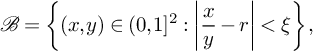 $$ \begin{align}\mathcal{B} = \left\{(x,y) \in (0,1]^2: \left|\frac{x}{y}-r\right|<\xi\right\},\end{align} $$
for a fixed real number $r>0$
and a small parameter
$r>0$
and a small parameter $\xi>0$
, and so we may choose
$\xi>0$
, and so we may choose $C=4$
, for example. We also define
$C=4$
, for example. We also define $\mathcal {B}N=\{(Nx,Ny): (x,y) \in \mathcal {B}\}.$
Let $\Delta $
be an integer and let
$\Delta $
be an integer and let $a_0,b_0 \in \mathbb {Z}/\Delta \mathbb {Z}$
. We now state the main sieve results which will be used in the proof of Theorem 1.1 and Theorem 1.3. They concern the sifting function
$a_0,b_0 \in \mathbb {Z}/\Delta \mathbb {Z}$
. We now state the main sieve results which will be used in the proof of Theorem 1.1 and Theorem 1.3. They concern the sifting function
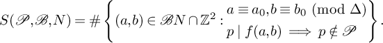 $$ \begin{align} S(\mathcal{P}, \mathcal{B},N) = \#\left\{(a,b)\in \mathcal{B}N\cap \mathbb{Z}^2: \begin{aligned} &a\equiv a_0, b\equiv b_0 \ (\mathrm{mod}\ \Delta)\\ &p\mid f(a,b) \implies p\notin \mathcal{P} \end{aligned} \right\}. \end{align} $$
Theorem 2.1. Let $f(x,y)$
be a binary form consisting of distinct irreducible factors, all of degree at most
$f(x,y)$
be a binary form consisting of distinct irreducible factors, all of degree at most $2$
. Then there exists a finite set of primes
$2$
. Then there exists a finite set of primes $S_0$
, depending on f, such that the following holds:
$S_0$
, depending on f, such that the following holds:
Let S be a finite set of primes containing $S_0$
. Let
$S_0$
. Let $\Delta $
be an integer with only prime factors in S, and let
$\Delta $
be an integer with only prime factors in S, and let $a_0, b_0 \in \mathbb {Z}/\Delta \mathbb {Z}$
. Let
$a_0, b_0 \in \mathbb {Z}/\Delta \mathbb {Z}$
. Let $\mathcal {P}$
be a set of primes disjoint from S and satisfying (2.4) and (2.5) for some
$\mathcal {P}$
be a set of primes disjoint from S and satisfying (2.4) and (2.5) for some $\alpha , \theta _i>0$
. Assume that
$\alpha , \theta _i>0$
. Assume that $\alpha \theta \leqslant 0.39$
. Then
$\alpha \theta \leqslant 0.39$
. Then $S(\mathcal {P},\mathcal {B},N)>0$
for N sufficiently large.
$S(\mathcal {P},\mathcal {B},N)>0$
for N sufficiently large.
We also have a similar sieve result when f may contain irreducible factors of degree up to $3$
, but with a less general sifting set
$3$
, but with a less general sifting set $\mathcal {P}$
, satisfying the following assumption.
$\mathcal {P}$
, satisfying the following assumption.
Assumption 2.2. There exists a positive integer n, a finite set of primes $S_0$
, primes
$S_0$
, primes $q_1, \ldots , q_n$
, and integers
$q_1, \ldots , q_n$
, and integers $t_1, \ldots , t_n$
with
$t_1, \ldots , t_n$
with $q_j \nmid t_j$
for all
$q_j \nmid t_j$
for all $j \in \{1, \ldots , n\}$
, such that
$j \in \{1, \ldots , n\}$
, such that
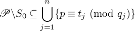 $$ \begin{align} \mathcal{P}\backslash S_0 \subseteq \bigcup_{j=1}^n \{p \equiv t_j \ (\mathrm{mod}\ q_j)\} \end{align} $$
and
 $$\begin{align*}\deg f \sum_{j=1}^n \frac{1}{q_j-1} \leqslant 0.32380. \end{align*}$$
Theorem 2.3. Let $f(x,y)$
be a binary form consisting of distinct irreducible factors, all of degree at most
$f(x,y)$
be a binary form consisting of distinct irreducible factors, all of degree at most $3$
. Then there exists a finite set of primes
$3$
. Then there exists a finite set of primes $S_0$
, depending on f, such that the following holds:
$S_0$
, depending on f, such that the following holds:
Let $\mathcal {P}$
be a set of primes satisfying Assumption 2.2 with the above choice of
$\mathcal {P}$
be a set of primes satisfying Assumption 2.2 with the above choice of $S_0$
. Let S be a finite set of primes containing
$S_0$
. Let S be a finite set of primes containing $S_0$
. Let
$S_0$
. Let $\Delta $
be an integer with only prime factors in S, and let
$\Delta $
be an integer with only prime factors in S, and let $a_0, b_0 \in \mathbb {Z}/\Delta \mathbb {Z}$
. Then
$a_0, b_0 \in \mathbb {Z}/\Delta \mathbb {Z}$
. Then $S(\mathcal {P}, \mathcal {B},N)>0$
for N sufficiently large.
$S(\mathcal {P}, \mathcal {B},N)>0$
for N sufficiently large.
For brevity, in the remainder of the paper, we shall denote the condition $a\equiv a_0 \ (\mathrm {mod}\ \Delta ), b\equiv b_0 \ (\mathrm {mod}\ \Delta )$
by
$a\equiv a_0 \ (\mathrm {mod}\ \Delta ), b\equiv b_0 \ (\mathrm {mod}\ \Delta )$
by $C(a,b)$
.
$C(a,b)$
.
3 Levels of distribution
Crucial to the success of the beta sieve in proving Theorems 2.1 and 2.3 is a good level of distribution result, which provides an approximation of the quantities
 $$ \begin{align*}\#\{(a,b) \in \mathcal{B}N\cap \mathbb{Z}^2: p\mid f_i(a,b), d \mid f(a,b)\}\end{align*} $$
by multiplicative functions, at least on average over p and d. (Here, and throughout this section, we keep the notation from Section 2.) In this section, we provide such an estimate, following similar arguments developed by Daniel [Reference Daniel15, Lemma 3.3]. We slightly generalise the setup as follows:
Let $g_1,g_2$
be binary forms with nonzero discriminants. Throughout this section, we fix
$g_1,g_2$
be binary forms with nonzero discriminants. Throughout this section, we fix $S, \Delta $
, and
$S, \Delta $
, and $C(a,b)$
, and assume that S contains all primes dividing the discriminants of
$C(a,b)$
, and assume that S contains all primes dividing the discriminants of $g_1$
and
$g_1$
and $g_2$
. We allow all implied constants to depend only the degrees of
$g_2$
. We allow all implied constants to depend only the degrees of $g_1$
and
$g_1$
and $g_2$
and a small positive constant
$g_2$
and a small positive constant $\epsilon $
, which for convenience, we allow to take different values at different points in the argument.
$\epsilon $
, which for convenience, we allow to take different values at different points in the argument.
Let $\mathcal {R}$
be a bounded region of
$\mathcal {R}$
be a bounded region of $\mathbb {R}^2$
whose boundary is a piecewise continuous simple closed curve of finite length. We denote by
$\mathbb {R}^2$
whose boundary is a piecewise continuous simple closed curve of finite length. We denote by $\operatorname {Vol}(\mathcal {R})$
and
$\operatorname {Vol}(\mathcal {R})$
and $P(\mathcal {R})$
the volume and perimeter of
$P(\mathcal {R})$
the volume and perimeter of $\mathcal {R}$
, respectively. Let
$\mathcal {R}$
, respectively. Let
 $$ \begin{align} A(d_1,d_2) &= \#\{(a,b)\in \mathcal{R}\cap \mathbb{Z}^2:C(a,b), d_1\mid g_1(a,b), d_2\mid g_2(a,b)\}, \end{align} $$
 $$ \begin{align} \varrho (d_1,d_2)&=\#\{(a,b) \ (\mathrm{mod}\ d_1d_2): d_1\mid g_1(a,b), d_2\mid g_2(a,b)\}. \quad\end{align} $$
We define
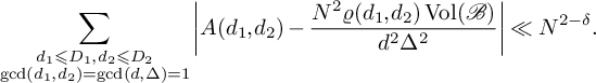
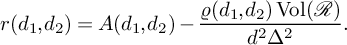 $$ \begin{align} r(d_1,d_2) = A(d_1,d_2)-\frac{\varrho (d_1,d_2)\operatorname{Vol}(\mathcal{R})}{d^2\Delta^2}. \end{align} $$
In what follows, we let $d=d_1d_2$
, and we assume that
$d=d_1d_2$
, and we assume that $\gcd (d_1,d_2)=\gcd (d,\Delta )=1$
. The main aim of this section is to prove the following proposition.
$\gcd (d_1,d_2)=\gcd (d,\Delta )=1$
. The main aim of this section is to prove the following proposition.
Proposition 3.1. Suppose that $g_1$
does not contain any linear factors. Then for any
$g_1$
does not contain any linear factors. Then for any $D_1,D_2>0$
and any
$D_1,D_2>0$
and any $\epsilon>0$
, we have
$\epsilon>0$
, we have
 $$ \begin{align*} \sum_{\substack{d_1\leqslant D_1, d_2\leqslant D_2\\ \gcd(d_1,d_2)=\gcd(d,\Delta)=1}}\sup_{P(\mathcal{R})\leqslant N}\left|r(d_1, d_2)\right|\ll (D_1D_2)^{\epsilon}(D_1D_2+N(D_1D_2)^{1/2}+ND_2). \end{align*} $$
As a corollary, we obtain the following level of distribution result.
Corollary 3.2. Suppose that $g_1$
does not contain any linear factors. Let
$g_1$
does not contain any linear factors. Let $\mathcal {B} \subseteq [-1,1]^2$
be as in Section 2, and let
$\mathcal {B} \subseteq [-1,1]^2$
be as in Section 2, and let $\mathcal {R} = \mathcal {B}N$
. Then for any
$\mathcal {R} = \mathcal {B}N$
. Then for any $\epsilon>0$
, there exists
$\epsilon>0$
, there exists $\delta>0$
such that for any
$\delta>0$
such that for any $D_1,D_2>0$
with
$D_1,D_2>0$
with $D_2 \ll N^{1-\epsilon }$
and
$D_2 \ll N^{1-\epsilon }$
and $D_1D_2 \ll N^{2-\epsilon }$
, we have
$D_1D_2 \ll N^{2-\epsilon }$
, we have
 $$ \begin{align} \sum_{\substack{d_1\leqslant D_1, d_2\leqslant D_2\\ \gcd(d_1,d_2)=\gcd(d,\Delta)=1}}\left|A(d_1,d_2)-\frac{N^2\varrho (d_1,d_2)\operatorname{Vol}(\mathcal{B})}{d^2\Delta^2}\right| \ll N^{2-\delta}. \end{align} $$
Proposition 3.1 and Corollary 3.2 are generalisations of Irving’s results from [Reference Irving27, Section 3], which can be recovered by taking $g_1(x,y) = f(x,y)$
to be the cubic form Irving considered, and
$g_1(x,y) = f(x,y)$
to be the cubic form Irving considered, and $g_2(x,y)=yf(x,y)$
. The method of proof is inspired by the pioneering work of Daniel on the divisor-sum problem for binary forms, which requires a similar level of distribution result (see [Reference Daniel15, Lemma 3.3]). Daniel’s argument is more delicate, keeping track of powers of
$g_2(x,y)=yf(x,y)$
. The method of proof is inspired by the pioneering work of Daniel on the divisor-sum problem for binary forms, which requires a similar level of distribution result (see [Reference Daniel15, Lemma 3.3]). Daniel’s argument is more delicate, keeping track of powers of $\log N$
in place of factors of
$\log N$
in place of factors of $N^{\epsilon }$
, and Corollary 3.2 could be similarly refined, but this yields no advantage for our applications.
$N^{\epsilon }$
, and Corollary 3.2 could be similarly refined, but this yields no advantage for our applications.
Before proceeding with the proof of Proposition 3.1, we recall the following standard lattice point counting result.
Lemma 3.3. Let $\Lambda \subseteq \mathbb {R}^2$
be a full-rank lattice, and let
$\Lambda \subseteq \mathbb {R}^2$
be a full-rank lattice, and let $\mathcal {R}\subseteq \mathbb {R}^2$
be as defined before Proposition 3.1. Then
$\mathcal {R}\subseteq \mathbb {R}^2$
be as defined before Proposition 3.1. Then
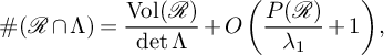 $$\begin{align*}\#(\mathcal{R}\cap \Lambda) = \frac{\operatorname{Vol}(\mathcal{R})}{\det \Lambda} + O\left(\frac{P(\mathcal{R})}{\lambda_1} + 1\right), \end{align*}$$
where $\lambda _1$
is the length of a shortest nonzero vector in
$\lambda _1$
is the length of a shortest nonzero vector in $\Lambda $
.
$\Lambda $
.
Proof. Let $\mathcal {F}$
be a fundamental domain of
$\mathcal {F}$
be a fundamental domain of $\Lambda $
. The translates
$\Lambda $
. The translates $v + \mathcal {F}$
for
$v + \mathcal {F}$
for $v \in \Lambda $
tile
$v \in \Lambda $
tile $\mathbb {R}^2$
. Define sets
$\mathbb {R}^2$
. Define sets
 $$\begin{align*}S^- = \{v \in \Lambda: (v + \mathcal{F}) \subseteq \mathcal{R}\}, \qquad S^+ = \{v \in \Lambda: (v + \mathcal{F})\cap \mathcal{R} \neq \emptyset\}. \end{align*}$$
Then
 $$\begin{align*}\frac{\operatorname{Vol}(S^-+ \Lambda)}{\det(\Lambda)} = \#S^- \leqslant \#(\mathcal{R}\cap \Lambda) \leqslant \#S^+ = \frac{\operatorname{Vol}(S^++ \Lambda)}{\det(\Lambda)}. \end{align*}$$
Moreover, $S^- + \Lambda \subseteq \mathcal {R} \subseteq S^+ + \Lambda $
, so
$S^- + \Lambda \subseteq \mathcal {R} \subseteq S^+ + \Lambda $
, so $\operatorname {Vol}(S^- + \Lambda ) \leqslant \operatorname {Vol}(\mathcal {R}) \leqslant \operatorname {Vol}( S^+ + \Lambda )$
. Therefore,
$\operatorname {Vol}(S^- + \Lambda ) \leqslant \operatorname {Vol}(\mathcal {R}) \leqslant \operatorname {Vol}( S^+ + \Lambda )$
. Therefore,
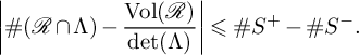 $$\begin{align*}\left|\#(\mathcal{R}\cap \Lambda) - \frac{\operatorname{Vol}(\mathcal{R})}{\det(\Lambda)}\right| \leqslant \#S^+ - \#S^-. \end{align*}$$
However, $S^+ - S^- = \{v \in \Lambda : (v + \mathcal {F}) \cap \partial \mathcal {R} \neq \emptyset \},$
where
$S^+ - S^- = \{v \in \Lambda : (v + \mathcal {F}) \cap \partial \mathcal {R} \neq \emptyset \},$
where $\partial \mathcal {R}$
denotes the boundary of
$\partial \mathcal {R}$
denotes the boundary of $\mathcal {R}$
. Each segment of
$\mathcal {R}$
. Each segment of $\partial \mathcal {R}$
of length
$\partial \mathcal {R}$
of length $\lambda _1$
can intersect at most four translates of
$\lambda _1$
can intersect at most four translates of $\mathcal {F}$
. Therefore,
$\mathcal {F}$
. Therefore, $S^+ - S^- \ll P(\mathcal {R})/\lambda _1 + 1$
, as required.
$S^+ - S^- \ll P(\mathcal {R})/\lambda _1 + 1$
, as required.
We now commence with the proof of Proposition 3.1. We introduce the quantities $R^*(d_1,d_2), \varrho ^*(d_1,d_2)$
and
$R^*(d_1,d_2), \varrho ^*(d_1,d_2)$
and $r^*(d_1,d_2)$
which are defined similarly to
$r^*(d_1,d_2)$
which are defined similarly to $A(d_1,d_2), \varrho (d_1,d_2)$
and
$A(d_1,d_2), \varrho (d_1,d_2)$
and $r(d_1,d_2)$
but with the added condition
$r(d_1,d_2)$
but with the added condition $\gcd (a,b,d)=1$
. We write
$\gcd (a,b,d)=1$
. We write $(a_1,b_1) \sim (a_2,b_2)$
if there exists an integer
$(a_1,b_1) \sim (a_2,b_2)$
if there exists an integer $\lambda $
such that
$\lambda $
such that $(a_1,b_1)\equiv \lambda (a_2,b_2)\ (\mathrm {mod}\ d)$
. This forms an equivalence relation on points
$(a_1,b_1)\equiv \lambda (a_2,b_2)\ (\mathrm {mod}\ d)$
. This forms an equivalence relation on points $(a,b)\in \mathbb {Z}^2$
with
$(a,b)\in \mathbb {Z}^2$
with $\gcd (a,b,d)=1$
. Moreover, the properties
$\gcd (a,b,d)=1$
. Moreover, the properties $g_1(a,b) \equiv 0 \ (\mathrm {mod}\ d_1)$
and
$g_1(a,b) \equiv 0 \ (\mathrm {mod}\ d_1)$
and $g_2(a,b)\equiv 0 \ (\mathrm {mod}\ d_2)$
are preserved under this equivalence. We may therefore define
$g_2(a,b)\equiv 0 \ (\mathrm {mod}\ d_2)$
are preserved under this equivalence. We may therefore define
 $$ \begin{align*}\mathcal{U}(d_1,d_2) = \left.\left\{a,b \ (\mathrm{mod}\ d): \begin{array}{l l} &\displaystyle \gcd(a,b,d)=1\\ &\displaystyle d_1\mid g_1(a,b), d_2\mid g_2(a,b) \end{array}\right\}\middle/\sim.\right.\end{align*} $$
For $\mathcal {C}\in \mathcal {U}(d_1,d_2)$
, we define
$\mathcal {C}\in \mathcal {U}(d_1,d_2)$
, we define
 $$ \begin{align*}\Lambda(\mathcal{C}) = \{y \in \mathbb{Z}^2: y \equiv \lambda(a,b) \ (\mathrm{mod}\ d)\textrm{ for some }(a,b)\in \mathcal{C} \textrm{ and some } \lambda \in \mathbb{Z}\}.\end{align*} $$
It is easy to check that $\Lambda (\mathcal {C})$
is a lattice in
$\Lambda (\mathcal {C})$
is a lattice in $\mathbb {Z}^2$
, and its set of primitive points is
$\mathbb {Z}^2$
, and its set of primitive points is $\mathcal {C}$
. For
$\mathcal {C}$
. For $e \in \mathbb {Z}$
, we define
$e \in \mathbb {Z}$
, we define
 $$ \begin{align*}\Lambda(\mathcal{C},e) = \{(a,b) \in \Lambda(\mathcal{C}): e\mid \gcd(a,b)\}.\end{align*} $$
By Möbius inversion, we have
 $$ \begin{align*}R^*(d_1,d_2) = \sum_{\mathcal{C} \in \mathcal{U}(d_1,d_2)}\sum_{e\mid d}\mu(e)\#\{(a,b) \in \mathcal{R}\cap \Lambda(\mathcal{C},e): C(a,b)\}.\end{align*} $$
Since $\gcd (d,\Delta )=1$
, the set
$\gcd (d,\Delta )=1$
, the set $\{(a,b) \in \Lambda (\mathcal {C},e):C(a,b)\}$
is a coset of the lattice
$\{(a,b) \in \Lambda (\mathcal {C},e):C(a,b)\}$
is a coset of the lattice $\Lambda (\mathcal {C},e\Delta )$
, which has determinant
$\Lambda (\mathcal {C},e\Delta )$
, which has determinant $de\Delta ^2$
. Therefore, by Lemma 3.3,
$de\Delta ^2$
. Therefore, by Lemma 3.3,
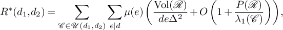 $$ \begin{align} R^*(d_1,d_2) = \sum_{\mathcal{C} \in \mathcal{U}(d_1,d_2)}\sum_{e\mid d}\mu(e) \left(\frac{\operatorname{Vol}(\mathcal{R})}{de\Delta^2}+O\left(1+\frac{P(\mathcal{R})}{\lambda_1(\mathcal{C})}\right)\right), \end{align} $$
where $\lambda _1(\mathcal {C})$
denotes the length of the shortest nonzero vector in
$\lambda _1(\mathcal {C})$
denotes the length of the shortest nonzero vector in $\Lambda (\mathcal {C})$
.
$\Lambda (\mathcal {C})$
.
Each equivalence class $\mathcal {C} \in \mathcal {U}(d_1,d_2)$
consists of
$\mathcal {C} \in \mathcal {U}(d_1,d_2)$
consists of $\varphi (d)$
elements, and so
$\varphi (d)$
elements, and so
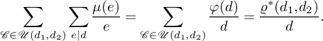 $$ \begin{align*}\sum_{\mathcal{C} \in \mathcal{U}(d_1,d_2)}\sum_{e\mid d}\frac{\mu(e)}{e} = \sum_{\mathcal{C} \in \mathcal{U}(d_1,d_2)}\frac{\varphi(d)}{d} = \frac{\varrho ^*(d_1,d_2)}{d}.\end{align*} $$
Moreover, we have $\#\mathcal {U}(d_1,d_2)\ll d^{\epsilon }$
, as we now explain. We observe that
$\#\mathcal {U}(d_1,d_2)\ll d^{\epsilon }$
, as we now explain. We observe that $\#\mathcal {U}(d_1,d_2) =\varrho ^*(d_1,d_2)/\varphi (d)$
, and
$\#\mathcal {U}(d_1,d_2) =\varrho ^*(d_1,d_2)/\varphi (d)$
, and $\varrho ^*$
is multiplicative by the Chinese remainder theorem. For primes
$\varrho ^*$
is multiplicative by the Chinese remainder theorem. For primes $p\notin S$
, we may apply Hensel’s lemma to show that
$p\notin S$
, we may apply Hensel’s lemma to show that $\varrho ^*(p^e,1),\varrho ^*(1,p^e) = O(p^e)$
for any integer
$\varrho ^*(p^e,1),\varrho ^*(1,p^e) = O(p^e)$
for any integer $e \geqslant 1$
. Therefore, by the trivial bound for the divisor function [Reference Hardy and Wright22, Section 18.1], we conclude that
$e \geqslant 1$
. Therefore, by the trivial bound for the divisor function [Reference Hardy and Wright22, Section 18.1], we conclude that
 $$ \begin{align} \#\mathcal{U}(d_1,d_2) = \frac{\varrho ^*(d_1,d_2)}{\varphi(d)}\ll \frac{d^{1+\epsilon}}{\varphi(d)}\ll d^{\epsilon}. \end{align} $$
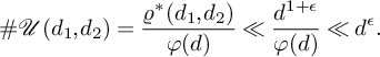
Applying (3.5), and (3.6), we obtain
 $$ \begin{align} \begin{aligned} &\sum_{\substack{d_1\leqslant D_1, d_2\leqslant D_2\\ \gcd(d_1,d_2)=\gcd(d,\Delta)=1}}\sup_{P(\mathcal{R})\leqslant N}\left|r^*(d_1,d_2)\right|\\ &\ll_{\epsilon}(D_1D_2)^{\epsilon}\left(D_1D_2+N\sum_{\substack{d_1\leqslant D_1, d_2\leqslant D_2\\ \gcd(d_1,d_2)= \gcd(d,\Delta)=1}}\sum_{\mathcal{C} \in \mathcal{U}(d_1,d_2)}\lambda_1(\mathcal{C})^{-1}\right). \end{aligned} \end{align} $$
Let $v_1(\mathcal {C})$
denote a shortest nonzero vector of
$v_1(\mathcal {C})$
denote a shortest nonzero vector of $\Lambda (\mathcal {C})$
, and let
$\Lambda (\mathcal {C})$
, and let $\|\cdot \|$
be the usual Euclidean norm. Then
$\|\cdot \|$
be the usual Euclidean norm. Then
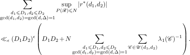
 $\|v_1(\mathcal {C})\|^2 \ll |\det \Lambda (\mathcal {C})|=d \leqslant D_1D_2$
. Therefore,
$\|v_1(\mathcal {C})\|^2 \ll |\det \Lambda (\mathcal {C})|=d \leqslant D_1D_2$
. Therefore,
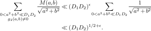
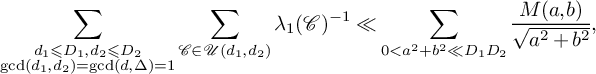 $$ \begin{align} \sum_{\substack{d_1\leqslant D_1, d_2\leqslant D_2\\ \gcd(d_1,d_2)=\gcd(d,\Delta)=1}}\sum_{\mathcal{C} \in \mathcal{U}(d_1,d_2)}\lambda_1(\mathcal{C})^{-1} \ll \sum_{0<a^2+b^2\ll D_1D_2}\frac{M(a,b)}{\sqrt{a^2+b^2}}, \end{align} $$
where

For any $d_1,d_2$
enumerated by
$d_1,d_2$
enumerated by $M(a,b)$
, we have
$M(a,b)$
, we have $d_1\mid g_1(a,b)$
and
$d_1\mid g_1(a,b)$
and $d_2\mid g_2(a,b)$
, so
$d_2\mid g_2(a,b)$
, so
 $$ \begin{align*}M(a,b) \leqslant \#\{d_1\leqslant D_1, d_2\leqslant D_2: d_1\mid g_1(a,b), d_2\mid g_2(a,b)\}.\end{align*} $$
Since $g_1$
contains no linear factors, we know that
$g_1$
contains no linear factors, we know that $g_1(a,b)\neq 0$
whenever
$g_1(a,b)\neq 0$
whenever $(a,b) \neq (0,0)$
. Suppose in addition that
$(a,b) \neq (0,0)$
. Suppose in addition that $g_2(a,b) \neq 0$
. Then by the trivial bound for the divisor function, we have
$g_2(a,b) \neq 0$
. Then by the trivial bound for the divisor function, we have $M(a,b) \ll (D_1D_2)^{\epsilon }$
. We deduce that
$M(a,b) \ll (D_1D_2)^{\epsilon }$
. We deduce that
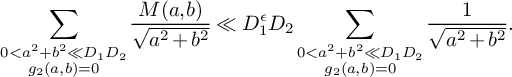
 $$ \begin{align*} \sum_{\substack{0<a^2+b^2\ll D_1D_2\\g_2(a,b)\neq 0}}\frac{M(a,b)}{\sqrt{a^2+b^2}}&\ll (D_1D_2)^{\epsilon}\sum_{0<a^2+b^2\ll D_1D_2}\frac{1}{\sqrt{a^2+b^2}}\\ &\ll (D_1D_2)^{1/2 + \epsilon}. \end{align*} $$
Now suppose that $g_2(a,b)=0$
. Then as above, we have
$g_2(a,b)=0$
. Then as above, we have $O(D_1^{\epsilon })$
choices for
$O(D_1^{\epsilon })$
choices for $d_1$
, but now
$d_1$
, but now $D_2$
choices for
$D_2$
choices for $d_2$
, so that
$d_2$
, so that $M(a,b) \ll D_1^{\epsilon }D_2$
. We obtain
$M(a,b) \ll D_1^{\epsilon }D_2$
. We obtain
 $$ \begin{align*} \sum_{\substack{0<a^2+b^2\ll D_1D_2\\g_2(a,b)= 0}}\frac{M(a,b)}{\sqrt{a^2+b^2}}&\ll D_1^{\epsilon}D_2\sum_{\substack{0<a^2+b^2\ll D_1D_2\\ g_2(a,b)=0}}\frac{1}{\sqrt{a^2+b^2}}. \end{align*} $$
For a fixed $b\neq 0$
,
$b\neq 0$
, $g_2(a,b)$
is a nonzero polynomial in a, and so has
$g_2(a,b)$
is a nonzero polynomial in a, and so has $O(1)$
roots. Therefore,
$O(1)$
roots. Therefore,
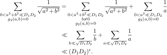 $$ \begin{align*} \sum_{\substack{0<a^2+b^2\ll D_1D_2\\ g_2(a,b)=0}}\frac{1}{\sqrt{a^2+b^2}}&= \sum_{ \substack{0<a^2+b^2\ll D_1D_2\\ b \neq 0\\g_2(a,b)= 0}}\frac{1}{\sqrt{a^2+b^2}}+\sum_{\substack{0<a^2 \ll D_1D_2\\ g_2(a,0)=0}}\frac{1}{a}\\ &\ll \sum_{b \ll \sqrt{D_1D_2}}\frac{1}{b}+\sum_{a \ll \sqrt{D_1D_2}}\frac{1}{a}\\ &\ll (D_1D_2)^{\epsilon}. \end{align*} $$
To summarize, we have established the following generalisation of [Reference Irving27, Lemma 3.2].
Lemma 3.4. Suppose that $g_1$
does not contain any linear factors. Then for any
$g_1$
does not contain any linear factors. Then for any $D_1,D_2>0$
and any
$D_1,D_2>0$
and any $\epsilon>0$
, we have
$\epsilon>0$
, we have
 $$ \begin{align*} \sum_{\substack{d_1\leqslant D_1, d_2\leqslant D_2\\ \gcd(d_1,d_2)= \gcd(d,\Delta)=1}}\sup_{P(\mathcal{R})\leqslant N}\left|r^*(d_1,d_2)\right|\ll (D_1D_2)^{\epsilon}(D_1D_2+N(D_1D_2)^{1/2}+ND_2). \end{align*} $$
Now we remove the restriction $\gcd (a,b,d)=1$
. Below, we write
$\gcd (a,b,d)=1$
. Below, we write $A(d_1,d_2)=A(\mathcal {R},d_1,d_2; C(a,b))$
in order to make the dependence on
$A(d_1,d_2)=A(\mathcal {R},d_1,d_2; C(a,b))$
in order to make the dependence on $\mathcal {R}$
and
$\mathcal {R}$
and $C(a,b)$
clear. Let
$C(a,b)$
clear. Let $k_1=\deg g_1$
and
$k_1=\deg g_1$
and $k_2=\deg g_2$
. We work with multiplicative functions
$k_2=\deg g_2$
. We work with multiplicative functions $\psi _k$
for
$\psi _k$
for $k=k_1$
and
$k=k_1$
and $k=k_2$
, which map prime powers
$k=k_2$
, which map prime powers $p^r$
to
$p^r$
to $p^{{\lceil r/k \rceil }}$
. We follow the same argument as Irving, but with
$p^{{\lceil r/k \rceil }}$
. We follow the same argument as Irving, but with $\psi _{k_1},\psi _{k_2}$
in place of
$\psi _{k_1},\psi _{k_2}$
in place of $\psi _3,\psi _4$
. The motivation for this definition of
$\psi _3,\psi _4$
. The motivation for this definition of $\psi _k$
comes from the fact that for any integers
$\psi _k$
comes from the fact that for any integers $d,e,k \geqslant 1$
with
$d,e,k \geqslant 1$
with $e\mid \psi _k(d)$
, and for any prime p, we have
$e\mid \psi _k(d)$
, and for any prime p, we have
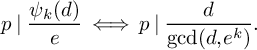 $$ \begin{align} p\mid \frac{\psi_k(d)}{e} \iff p \mid \frac{d}{\gcd(d,e^k)}. \end{align} $$
Since $\gcd (d_1,d_2)=1$
, we have
$\gcd (d_1,d_2)=1$
, we have
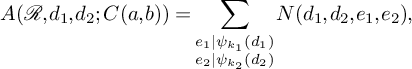 $$ \begin{align} A(\mathcal{R},d_1,d_2;C(a,b)) = \sum_{\substack{e_1\mid \psi_{k_1}(d_1)\\e_2\mid \psi_{k_2}(d_2)}}N(d_1,d_2,e_1,e_2), \end{align} $$
where
 $$ \begin{align} N(d_1,d_2,e_1,e_2) = \#\left\{(a,b) \in \mathcal{R}\cap \mathbb{Z}^2: \begin{array}{l l} &\displaystyle C(a,b), d_1\mid g_1(a,b), d_2\mid g_2(a,b),\\ &\displaystyle \gcd(a,b,\psi_{k_1}(d_1)\psi_{k_2}(d_2)) = e_1e_2 \end{array} \right\}. \end{align} $$
We make a change of variables $a' = a/e_1e_2, b' = b/e_1e_2$
in (3.11). Let
$a' = a/e_1e_2, b' = b/e_1e_2$
in (3.11). Let $\overline {e_1e_2}$
denote the multiplicative inverse of
$\overline {e_1e_2}$
denote the multiplicative inverse of $e_1e_2$
modulo
$e_1e_2$
modulo $\Delta $
, which exists due to the assumption
$\Delta $
, which exists due to the assumption $\gcd (d_1d_2, \Delta )=1$
. The congruence condition
$\gcd (d_1d_2, \Delta )=1$
. The congruence condition $C(a,b)$
is equivalent to the congruence condition
$C(a,b)$
is equivalent to the congruence condition $a' \equiv \overline {e_1e_2}a_0 \ (\mathrm {mod}\ \Delta )$
and
$a' \equiv \overline {e_1e_2}a_0 \ (\mathrm {mod}\ \Delta )$
and $b' \equiv \overline {e_1e_2}b_0\ (\mathrm {mod}\ \Delta )$
, which we denote by
$b' \equiv \overline {e_1e_2}b_0\ (\mathrm {mod}\ \Delta )$
, which we denote by $C'(a',b')$
. We have
$C'(a',b')$
. We have
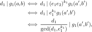 $$ \begin{align*} d_1\mid g_1(a,b) &\iff d_1 \mid (e_1e_2)^{k_1} g_1(a',b') \\ &\iff d_1 \mid e_1^{k_1}g_1(a',b') \\ &\iff \frac{d_1}{\gcd(d_1,e_1^{k_1})}\mid g_1(a',b'), \end{align*} $$
and similarly for $d_2 \mid g_2(a,b)$
. For convenience, we define
$d_2 \mid g_2(a,b)$
. For convenience, we define
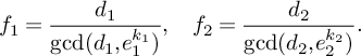 $$ \begin{align*}f_1 = \frac{d_1}{\gcd(d_1,e_1^{k_1})}, \quad f_2 =\frac{d_2}{\gcd(d_2,e_2^{k_2})}.\end{align*} $$
Changing notation from $a',b'$
back to
$a',b'$
back to $a,b$
, we deduce that
$a,b$
, we deduce that $N(d_1,d_2,e_1,e_2)$
can be rewritten as
$N(d_1,d_2,e_1,e_2)$
can be rewritten as
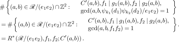 $$ \begin{align} &\#\left\{(a,b) \in \mathcal{R}/(e_1e_2)\cap \mathbb{Z}^2: \begin{array}{l l} &\displaystyle C'(a,b), f_1\mid g_1(a,b), f_2\mid g_2(a,b), \nonumber\\ &\displaystyle \gcd(a,b,\psi_{k_1}(d_1)\psi_{k_2}(d_2)/e_1e_2) = 1 \end{array} \right\}\\ &=\#\left\{(a,b) \in \mathcal{R}/(e_1e_2)\cap \mathbb{Z}^2: \begin{array}{l l} &\displaystyle C'(a,b), f_1\mid g_1(a,b), f_2\mid g_2(a,b),\\ &\displaystyle \gcd(a,b,f_1f_2)= 1 \end{array} \right\}.\nonumber\\ &=R^*\left(\mathcal{R}/(e_1e_2), f_1,f_2;C'(a,b)\right). \end{align} $$
The above arguments, but with the congruence conditions removed, and with the specific choice $\mathcal {R} = [0,d_1d_2]^2$
also demonstrate that
$\mathcal {R} = [0,d_1d_2]^2$
also demonstrate that
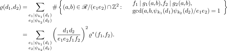 $$ \begin{align} \varrho (d_1,d_2) &=\sum_{\substack{e_1\mid \psi_{k_1}(d_1)\\e_2\mid \psi_{k_2}(d_2)}}\#\left\{(a,b) \in \mathcal{R}/(e_1e_2)\cap \mathbb{Z}^2:\begin{array}{l l} &\displaystyle f_1\mid g_1(a,b), f_2\mid g_2(a,b),\nonumber\\ &\displaystyle \gcd(a,b,\psi_{k_1}(d_1)\psi_{k_2}(d_2)/e_1e_2) = 1 \end{array} \right\}\\ &= \sum_{\substack{e_1\mid \psi_{k_1}(d_1)\\e_2\mid \psi_{k_2}(d_2)}}\left(\frac{d_1d_2}{e_1e_2f_1f_2}\right)^2\varrho ^*(f_1,f_2). \end{align} $$
We denote the quantity
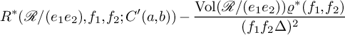 $$ \begin{align*}R^*(\mathcal{R}/(e_1e_2), f_1,f_2; C'(a,b)) - \frac{\operatorname{Vol}(\mathcal{R}/(e_1e_2))\varrho ^*(f_1,f_2)}{(f_1f_2\Delta)^2}\end{align*} $$
by $E(e_1,e_2,f_1,f_2)$
. Combining (3.10), (3.12) and (3.13), we have
$E(e_1,e_2,f_1,f_2)$
. Combining (3.10), (3.12) and (3.13), we have
 $$ \begin{align} &\sum_{\substack{d_1\leqslant D_1,d_2\leqslant D_2\\ (d_1,d_2)=(d_1d_2,\Delta)=1}}\sup_{P(\mathcal{R})\leqslant N}\left|r(d_1,d_2)\right|=\sum_{\substack{d_1\leqslant D_1,d_2\leqslant D_2\\ (d_1,d_2)=(d_1d_2,\Delta)=1}}\sup_{P(\mathcal{R})\leqslant N}\sum_{\substack{e_1\mid \psi_{k_1}(d_1)\\e_2\mid \psi_{k_2}(d_2)}}|E(e_1,e_2,f_1,f_2)| \end{align} $$
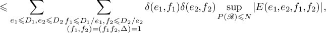 $$ \begin{align} &\leqslant \sum_{e_1\leqslant D_1,e_2\leqslant D_2}\sum_{\substack{f_1\leqslant D_1/e_1, f_2 \leqslant D_2/e_2\\ (f_1,f_2) = (f_1f_2,\Delta) =1}}\delta(e_1,f_1)\delta(e_2,f_2)\sup_{P(\mathcal{R})\leqslant N}\left|E(e_1,e_2,f_1,f_2)\right|, \end{align} $$
where for integers $e,f,k,D \geqslant 1$
, we have defined
$e,f,k,D \geqslant 1$
, we have defined
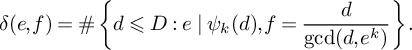 $$ \begin{align*}\delta(e,f) = \#\left\{d\leqslant D: e\mid \psi_{k}(d), f = \frac{d}{\gcd(d,e^{k})}\right\}.\end{align*} $$
We claim that $\delta (e,f) \ll e^{\epsilon }$
. To see this, suppose that p is a prime and let
$\delta (e,f) \ll e^{\epsilon }$
. To see this, suppose that p is a prime and let $r=\nu _p(d), s=\nu _p(e)$
and
$r=\nu _p(d), s=\nu _p(e)$
and $t = \nu _p(f)$
. There is a unique choice of r for a given
$t = \nu _p(f)$
. There is a unique choice of r for a given $k,s$
and t provided that
$k,s$
and t provided that $t>0$
– namely,
$t>0$
– namely, $r=ks+t$
. If
$r=ks+t$
. If $t=0$
, then we deduce from
$t=0$
, then we deduce from $f = d/\gcd (d,e^{k})$
that
$f = d/\gcd (d,e^{k})$
that $r\leqslant ks$
. Taking a product over primes, we conclude that each d enumerated by
$r\leqslant ks$
. Taking a product over primes, we conclude that each d enumerated by $\delta (e,f)$
is a divisor of
$\delta (e,f)$
is a divisor of $e^k$
multiplied by a quantity that is uniquely determined by e and f. The claim follows since the number of divisors of
$e^k$
multiplied by a quantity that is uniquely determined by e and f. The claim follows since the number of divisors of $e^k$
is
$e^k$
is $O(e^{\epsilon })$
. In our situation, where
$O(e^{\epsilon })$
. In our situation, where $e_1\leqslant D_1$
and
$e_1\leqslant D_1$
and $e_2 \leqslant D_2$
, we obtain
$e_2 \leqslant D_2$
, we obtain $\delta (e_1,f_1)\delta (e_2,f_2) \ll (D_1D_2)^{\epsilon }.$
Therefore, applying Lemma 3.4 for each choice of
$\delta (e_1,f_1)\delta (e_2,f_2) \ll (D_1D_2)^{\epsilon }.$
Therefore, applying Lemma 3.4 for each choice of $e_1,e_2$
in (3.15), we conclude that
$e_1,e_2$
in (3.15), we conclude that
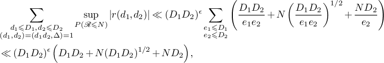 $$ \begin{align*} &\sum_{\substack{d_1\leqslant D_1,d_2\leqslant D_2\\ (d_1,d_2)=(d_1d_2,\Delta)=1}}\sup_{P(\mathcal{R}\leqslant N)}\left|r(d_1,d_2)\right|\ll (D_1D_2)^{\epsilon}\sum_{\substack{e_1\leqslant D_1\\e_2\leqslant D_2}}\left(\frac{D_1D_2}{e_1e_2}+N\left(\frac{D_1D_2}{e_1e_2}\right)^{1/2}+\frac{ND_2}{e_2}\right)\\ &\ll (D_1D_2)^{\epsilon}\left(D_1D_2 + N(D_1D_2)^{1/2}+ND_2\right), \end{align*} $$
which completes the proof of Proposition 3.1.
Remark 3.5. If $g_2(a,b)\neq 0$
for all
$g_2(a,b)\neq 0$
for all $(a,b) \neq (0,0)$
, then we do not need to consider the case
$(a,b) \neq (0,0)$
, then we do not need to consider the case $g_2(a,b)=0$
in the analysis of the sum in (3.8), and so in our final level of distribution result, we do not require the assumption
$g_2(a,b)=0$
in the analysis of the sum in (3.8), and so in our final level of distribution result, we do not require the assumption $D_2 \ll N^{1-\epsilon }$
.
$D_2 \ll N^{1-\epsilon }$
.
When $g_1(a,b)$
does contain linear factors, we can still obtain a basic level of distribution result from the above argument using the trivial estimate
$g_1(a,b)$
does contain linear factors, we can still obtain a basic level of distribution result from the above argument using the trivial estimate $\lambda _1(\mathcal {C})^{-1}\leqslant 1$
in (3.7). This establishes the following lemma.
$\lambda _1(\mathcal {C})^{-1}\leqslant 1$
in (3.7). This establishes the following lemma.
Lemma 3.6. Let $g_1,g_2$
be arbitrary binary forms with nonzero discriminant. Then for any
$g_1,g_2$
be arbitrary binary forms with nonzero discriminant. Then for any $\epsilon>0$
, there exists
$\epsilon>0$
, there exists $\delta>0$
such that for any
$\delta>0$
such that for any $D_1,D_2>0$
with
$D_1,D_2>0$
with $D_1D_2 \ll N^{1-\epsilon }$
, we have
$D_1D_2 \ll N^{1-\epsilon }$
, we have
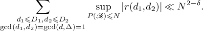 $$ \begin{align*}\sum_{\substack{d_1\leqslant D_1, d_2\leqslant D_2\\ \gcd(d_1,d_2)=\gcd(d,\Delta)=1}}\sup_{P(\mathcal{R})\leqslant N}\left|r(d_1,d_2)\right| \ll N^{2-\delta}.\end{align*} $$
4 Application of the beta sieve
In this section, we prove Theorem 2.1 and Theorem 2.3 by combining the level of distribution results from Section 3 with the beta sieve of Rosser and Iwaniec [Reference Friedlander and Iwaniec18, Theorem 11.12]. We state the precise version of this theorem we need in Theorem 4.1.
We recall some of the notation from Section 2. We fix a region $\mathcal {R}=\mathcal {B}N$
for some
$\mathcal {R}=\mathcal {B}N$
for some $\mathcal {B}\subseteq [-1,1]^2$
as in Section 2. Then
$\mathcal {B}\subseteq [-1,1]^2$
as in Section 2. Then $\mathcal {R}$
has volume
$\mathcal {R}$
has volume $\gg N^2$
and perimeter
$\gg N^2$
and perimeter $\ll N$
. Let d denote the largest degree among the irreducible factors of f. (We specialise to the cases
$\ll N$
. Let d denote the largest degree among the irreducible factors of f. (We specialise to the cases $d=2$
and
$d=2$
and $d=3$
later. The reason our methods are unable to deal with larger values of d is explained in Remark 4.5.) Then there exists
$d=3$
later. The reason our methods are unable to deal with larger values of d is explained in Remark 4.5.) Then there exists $x \ll N^d$
such that the largest prime factor of
$x \ll N^d$
such that the largest prime factor of $f(a,b)$
for
$f(a,b)$
for $(a,b)\in \mathcal {R}\cap \mathbb {Z}^2$
is strictly less than x. Let S be a finite set of primes, including all primes dividing the discriminant of
$(a,b)\in \mathcal {R}\cap \mathbb {Z}^2$
is strictly less than x. Let S be a finite set of primes, including all primes dividing the discriminant of $f(x,y)$
. In Section 4.6, we also append to S all primes bounded by some constant
$f(x,y)$
. In Section 4.6, we also append to S all primes bounded by some constant $P_1$
. Let
$P_1$
. Let $\Delta $
be an integer with only prime factors in S. Without loss of generality, we may assume every prime in S divides
$\Delta $
be an integer with only prime factors in S. Without loss of generality, we may assume every prime in S divides $\Delta $
because taking a multiple of
$\Delta $
because taking a multiple of $\Delta $
can only decrease the sifting function
$\Delta $
can only decrease the sifting function $S(\mathcal {P}, \mathcal {B}, N)$
from (4.2). Additionally, by taking an appropriate multiple of
$S(\mathcal {P}, \mathcal {B}, N)$
from (4.2). Additionally, by taking an appropriate multiple of $\Delta $
and appropriate lifts of
$\Delta $
and appropriate lifts of $a_0, b_0$
, we may assume that
$a_0, b_0$
, we may assume that $\nu _p(f(a_0, b_0)) < \nu _p(\Delta )$
for all
$\nu _p(f(a_0, b_0)) < \nu _p(\Delta )$
for all $p\in S$
.
$p\in S$
.
All implied constants in this section are allowed to depend on $\Delta $
. Let
$\Delta $
. Let $\mathcal {P}$
be a set of primes disjoint from S satisfying (2.4) and (2.5). We also define
$\mathcal {P}$
be a set of primes disjoint from S satisfying (2.4) and (2.5). We also define $\mathcal {P'}$
to be the set of primes not in
$\mathcal {P'}$
to be the set of primes not in $\mathcal {P}\cup S$
. Let
$\mathcal {P}\cup S$
. Let $P(x)$
denote the product of primes in
$P(x)$
denote the product of primes in $\mathcal {P}_{< x}$
, and similarly for
$\mathcal {P}_{< x}$
, and similarly for $P'(x)$
. We also define
$P'(x)$
. We also define $X = \operatorname {Vol}(\mathcal {R})/\Delta ^2$
.
$X = \operatorname {Vol}(\mathcal {R})/\Delta ^2$
.
For a sequence of non-negative real numbers $\mathcal {A} = (a_n)$
, and a parameter
$\mathcal {A} = (a_n)$
, and a parameter $z\geqslant 1$
, we define the sifting function
$z\geqslant 1$
, we define the sifting function
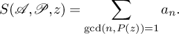 $$ \begin{align*}S(\mathcal{A}, \mathcal{P}, z) = \sum_{\gcd(n,P(z))=1}a_n.\end{align*} $$
We make the choice
 $$ \begin{align} a_n = \#\{(a,b) \in \mathcal{R}\cap \mathbb{Z}^2: C(a,b), f(a,b) = n\}, \end{align} $$
so that
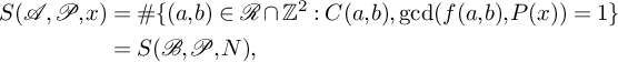 $$ \begin{align} \begin{aligned} S(\mathcal{A},\mathcal{P},x)&=\#\{(a,b)\in \mathcal{R}\cap \mathbb{Z}^2: C(a,b), \gcd(f(a,b), P(x))=1\}\\ &=S(\mathcal{B},\mathcal{P},N), \end{aligned} \end{align} $$
where $S(\mathcal {B},\mathcal {P},N)$
is as defined in (2.8). Our aim is to prove that
$S(\mathcal {B},\mathcal {P},N)$
is as defined in (2.8). Our aim is to prove that $S(\mathcal {A}, \mathcal {P}, x)>0$
for sufficiently large N (which may depend on
$S(\mathcal {A}, \mathcal {P}, x)>0$
for sufficiently large N (which may depend on $\Delta $
). For a prime
$\Delta $
). For a prime $p\in \mathcal {P}$
and for any
$p\in \mathcal {P}$
and for any $i\in \{0,\ldots , k\}$
, we also consider the sequences
$i\in \{0,\ldots , k\}$
, we also consider the sequences $\mathcal {A}_p, \mathcal {A}_p^{(i)}$
defined similarly to (4.1) but with the additional conditions
$\mathcal {A}_p, \mathcal {A}_p^{(i)}$
defined similarly to (4.1) but with the additional conditions $p\mid f(a,b), p\mid f_i(a,b)$
, respectively, so that
$p\mid f(a,b), p\mid f_i(a,b)$
, respectively, so that
 $$ \begin{align*} S(\mathcal{A}_p, \mathcal{P}, p) &=\#\{(a,b)\in \mathcal{R}\cap \mathbb{Z}^2: C(a,b), p\mid f(a,b), \gcd(f(a,b), P(p))=1\},\\ S(\mathcal{A}_p^{(i)}, \mathcal{P},p) &=\#\{(a,b)\in \mathcal{R}\cap \mathbb{Z}^2: C(a,b), p\mid f_i(a,b), \gcd(f(a,b), P(p))=1\}. \end{align*} $$
Using the Buchstab identity, we have
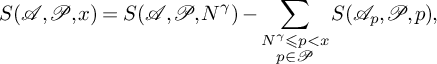 $$ \begin{align*}S(\mathcal{A},\mathcal{P},x) = S(\mathcal{A},\mathcal{P},N^{\gamma})-\sum_{\substack{N^{\gamma} \leqslant p < x\\p \in \mathcal{P}}}S(\mathcal{A}_p, \mathcal{P},p),\end{align*} $$
for a parameter $\gamma \in (0,1)$
to be chosen later. We denote
$\gamma \in (0,1)$
to be chosen later. We denote $S(\mathcal {A},\mathcal {P},N^{\gamma })$
by
$S(\mathcal {A},\mathcal {P},N^{\gamma })$
by $S_1$
. If
$S_1$
. If $p\mid f(a,b)$
, then
$p\mid f(a,b)$
, then $p\mid f_i(a,b)$
for some i. Therefore, we have the decomposition
$p\mid f_i(a,b)$
for some i. Therefore, we have the decomposition
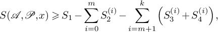 $$ \begin{align*}S(\mathcal{A},\mathcal{P},x) \geqslant S_1 -\sum_{i=0}^m S_2^{(i)}- \sum_{i=m+1}^k \left(S_3^{(i)}+S_4^{(i)}\right),\end{align*} $$
where
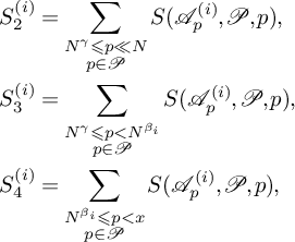 $$ \begin{align} \begin{aligned} S_2^{(i)} &=\sum_{\substack{N^{\gamma}\leqslant p \ll N\\p \in \mathcal{P}}}S(\mathcal{A}_p^{(i)},\mathcal{P},p),\\ S_3^{(i)}&=\sum_{\substack{N^{\gamma}\leqslant p < N^{\beta_i}\\p \in \mathcal{P}}}S(\mathcal{A}_p^{(i)}, \mathcal{P},p), \\ S_4^{(i)}&=\sum_{\substack{N^{\beta_i}\leqslant p< x\\p \in \mathcal{P}}}S(\mathcal{A}_p^{(i)}, \mathcal{P},p), \end{aligned} \end{align} $$
for parameters $\beta _i\geqslant \gamma $
to be chosen later.
$\beta _i\geqslant \gamma $
to be chosen later.
4.1 The beta sieve
Like most combinatorial sieves, the beta sieve provides a mechanism to estimate sifting functions of the form $S(\mathcal {A},\mathcal {P},z)$
given arithmetic information about the related quantities
$S(\mathcal {A},\mathcal {P},z)$
given arithmetic information about the related quantities $|\mathcal {A}_d| := \sum _{d\mid n}a_n$
for squarefree integers d. More specifically, we require an approximation
$|\mathcal {A}_d| := \sum _{d\mid n}a_n$
for squarefree integers d. More specifically, we require an approximation $|\mathcal {A}_d| = |\mathcal {A}_1|g(d) + r(d)$
, where
$|\mathcal {A}_d| = |\mathcal {A}_1|g(d) + r(d)$
, where $g(d)$
is a multiplicative function supported on squarefree integers and
$g(d)$
is a multiplicative function supported on squarefree integers and
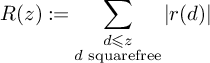 $$\begin{align*}R(z) := \sum_{\substack{d\leqslant z\\ d \textrm{ squarefree}}}|r(d)| \end{align*}$$
is small. Define
 $$ \begin{align*}V(z) = \sum_{d \mid P(z)}\mu(d)g(d) = \prod_{p \in \mathcal{P}_{\leqslant z}}(1-g(p)).\end{align*} $$
We shall assume that for some $\kappa , L \geqslant 0$
, we have
$\kappa , L \geqslant 0$
, we have
 $$ \begin{align} V(w) \leqslant \left(\frac{\log z}{\log w}\right)^{\kappa}\left(1+\frac{L}{\log w}\right)V(z) \end{align} $$
for all $2 \leqslant w \leqslant z$
.
$2 \leqslant w \leqslant z$
.
For some choice of sieve weights $\Lambda ^{\pm } =(\lambda _d^{\pm })_{d \geqslant 1}$
, define
$\Lambda ^{\pm } =(\lambda _d^{\pm })_{d \geqslant 1}$
, define
 $$\begin{align*}V^{\pm}(z) = \sum_{d\mid P(z)}\lambda_d^{\pm}g(d). \end{align*}$$
We recall that if $\Lambda ^{\pm }$
are upper and lower bound sieves of level z (i.e., if
$\Lambda ^{\pm }$
are upper and lower bound sieves of level z (i.e., if $\lambda ^{\pm }_d$
are supported on squarefree integers
$\lambda ^{\pm }_d$
are supported on squarefree integers $d<z$
and
$d<z$
and
 $$\begin{align*}\sum_{d\mid m}\lambda^-_d \leqslant \sum_{d\mid m}\mu(d) \leqslant \sum_{d\mid m}\lambda^+_d \end{align*}$$
for all integers m), then we have
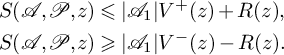 $$ \begin{align} \begin{aligned} S(\mathcal{A}, \mathcal{P}, z) &\leqslant |\mathcal{A}_1|V^+(z) + R(z),\\ S(\mathcal{A}, \mathcal{P}, z) &\geqslant |\mathcal{A}_1|V^-(z) - R(z). \end{aligned} \end{align} $$
The main theorem of the beta sieve we apply is given in [Reference Friedlander and Iwaniec18, Theorem 11.12]. We record this theorem here for convenience, in the special case $s=1$
.
$s=1$
.
Theorem 4.1. Suppose $\kappa , L$
are such that the assumption (4.4) holds. Then there is a choice of upper and lower bound sieve weights
$\kappa , L$
are such that the assumption (4.4) holds. Then there is a choice of upper and lower bound sieve weights $\Lambda ^{\pm }$
(taking values in
$\Lambda ^{\pm }$
(taking values in $\{-1,0,1\}$
), and explicit constants
$\{-1,0,1\}$
), and explicit constants $A(\kappa ), B(\kappa ) \geqslant 0$
such that, as
$A(\kappa ), B(\kappa ) \geqslant 0$
such that, as $z\rightarrow \infty $
, we have
$z\rightarrow \infty $
, we have
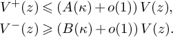 $$ \begin{align} \begin{aligned} V^+(z) &\leqslant \left(A(\kappa) + o(1)\right)V(z),\\ V^-(z) &\geqslant \left(B(\kappa) + o(1)\right)V(z). \end{aligned} \end{align} $$
Notation 4.2. Throughout the remainder of this chapter, for a sequence $\mathcal {A}$
, a set of primes
$\mathcal {A}$
, a set of primes $\mathcal {P}$
, a multiplicative function g, and a sifting level
$\mathcal {P}$
, a multiplicative function g, and a sifting level $z\geqslant 1$
, we define
$z\geqslant 1$
, we define $\Lambda ^{\pm }(\mathcal {A},\mathcal {P},g,z)$
to be the corresponding upper and lower bound beta sieves with these parameters. We sometimes apply (4.6) directly without reference to a sequence, in which case the parameter
$\Lambda ^{\pm }(\mathcal {A},\mathcal {P},g,z)$
to be the corresponding upper and lower bound beta sieves with these parameters. We sometimes apply (4.6) directly without reference to a sequence, in which case the parameter $\mathcal {A}$
is omitted from the notation.
$\mathcal {A}$
is omitted from the notation.
In our applications of the beta sieve, the required bounds on $R(z)$
are provided by Corollary 3.2 and Lemma 3.6. For
$R(z)$
are provided by Corollary 3.2 and Lemma 3.6. For $i\in \{0,\ldots , k\}$
, we define multiplicative functions
$i\in \{0,\ldots , k\}$
, we define multiplicative functions
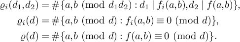 $$ \begin{align*} \varrho _i(d_1,d_2) &=\#\{a,b \ (\mathrm{mod}\ d_1d_2): d_1\mid f_i(a,b), d_2\mid f(a,b)\},\\ \varrho _i(d) &=\#\{a,b \ (\mathrm{mod}\ d): f_i(a,b) \equiv 0 \ (\mathrm{mod}\ d)\},\\ \varrho (d) &= \#\{a,b \ (\mathrm{mod}\ d): f(a,b) \equiv 0 \ (\mathrm{mod}\ d)\}. \end{align*} $$
We note that the function $\varrho _i(d_1,d_2)$
is the same as the function
$\varrho _i(d_1,d_2)$
is the same as the function $\varrho (d_1,d_2)$
from (3.2) with
$\varrho (d_1,d_2)$
from (3.2) with $g_1(x,y) = f_i(x,y)$
and
$g_1(x,y) = f_i(x,y)$
and $g_2(x,y) = f(x,y)$
, but in this section, we add a subscript to keep track of the dependence on i. When
$g_2(x,y) = f(x,y)$
, but in this section, we add a subscript to keep track of the dependence on i. When $\gcd (d_1,d_2) = 1$
, we have
$\gcd (d_1,d_2) = 1$
, we have $\varrho _i(d_1,d_2) = \varrho _i(d_1)\varrho (d_2)$
. Moreover, for any
$\varrho _i(d_1,d_2) = \varrho _i(d_1)\varrho (d_2)$
. Moreover, for any $i\in \{1,\ldots , k\}$
and any prime
$i\in \{1,\ldots , k\}$
and any prime $p\notin S$
, we have
$p\notin S$
, we have
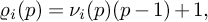 $$ \begin{align} \varrho _i(p) &= \nu_i(p)(p-1)+1, \end{align} $$
 $$ \begin{align} \varrho (p) &= \nu(p)(p-1)+1, \end{align} $$
where $\nu _i(p)$
and
$\nu _i(p)$
and $\nu (p)$
are as defined in (2.2) and (2.3). We define multiplicative functions
$\nu (p)$
are as defined in (2.2) and (2.3). We define multiplicative functions
 $$\begin{align*}g(p) := \frac{\varrho (p)}{p^2}, \qquad g_i(p) := \frac{\varrho _i(p)}{p^2} \end{align*}$$
and define
 $$ \begin{align} V(x)= \prod_{\substack{p\in \mathcal{P}_{\leqslant z}}}\left(1-g(p)\right), \qquad V_i(x)= \prod_{\substack{p\in \mathcal{P}^{\prime}_{\leqslant z}}}\left(1-g_i(p)\right) \end{align} $$
for $i\in \{1,\ldots , k\}$
.
$i\in \{1,\ldots , k\}$
.
4.2 Sieve dimensions
We prove in Lemma 4.3 that the functions $V,V_i$
defined above satisfy the hypothesis (4.4) with the sieve dimensions
$V,V_i$
defined above satisfy the hypothesis (4.4) with the sieve dimensions
where $\alpha , \theta _i$
and
$\alpha , \theta _i$
and $\theta $
are as defined in (2.4), (2.5) and (2.6).
$\theta $
are as defined in (2.4), (2.5) and (2.6).
In the notation of Theorem 4.1, we write $A=A(\kappa ), B=B(\kappa )$
and
$A=A(\kappa ), B=B(\kappa )$
and $A_i = A(\kappa _i)$
. We assume throughout this section that
$A_i = A(\kappa _i)$
. We assume throughout this section that $\kappa <1/2$
, and so
$\kappa <1/2$
, and so $\kappa _i>1/2$
. Then A and B are defined in [Reference Friedlander and Iwaniec18, Equations (11.62, 11.63)] (see also Section 4.9), and
$\kappa _i>1/2$
. Then A and B are defined in [Reference Friedlander and Iwaniec18, Equations (11.62, 11.63)] (see also Section 4.9), and $A_i$
is defined in [Reference Friedlander and Iwaniec18, Equations (11.42), (11.57)]. A table of numerical values of these constants can be found in [Reference Friedlander and Iwaniec18, Section 11.19].
$A_i$
is defined in [Reference Friedlander and Iwaniec18, Equations (11.42), (11.57)]. A table of numerical values of these constants can be found in [Reference Friedlander and Iwaniec18, Section 11.19].
Lemma 4.3. Let $x\geqslant 1$
. For
$x\geqslant 1$
. For $i\in \{1,\ldots ,k\}$
, and
$i\in \{1,\ldots ,k\}$
, and $V,V_i$
as in (4.9), there exist constants
$V,V_i$
as in (4.9), there exist constants $c,c_i>0$
such that
$c,c_i>0$
such that
 $$ \begin{align} V(x)&= \frac{c}{(\log x)^{\kappa}}\left(1+O((\log x)^{-1})\right), \end{align} $$
 $$ \begin{align} V_i(x)&= \frac{c_i}{(\log x)^{\kappa_i}}\left(1+O((\log x)^{-1})\right). \end{align} $$
The asymptotic in (4.11) also holds for $i=0$
when
$i=0$
when $f_0 \not \equiv 1$
.
$f_0 \not \equiv 1$
.
Proof. We follow a similar approach to [Reference Irving27, Lemma 4.2]. Below, we denote by C a constant which is allowed to vary from line to line. We have
 $$ \begin{align} \log V(x)&=-\sum_{p \in \mathcal{P}_{\leqslant x}}\left(\sum_{m=1}^{\infty}\frac{\varrho (p)^m}{mp^ {2m}}\right) \end{align} $$
 $$ \begin{align} &=-\sum_{p\in \mathcal{P}_{\leqslant x}}\frac{\nu(p)(p-1)+1}{p^2} + C + O((\log x)^{-1}). \end{align} $$
 $$ \begin{align} &=-\sum_{p\in \mathcal{P}_{\leqslant x}}\frac{\nu(p)}{p} + C + O((\log x)^{-1}), \end{align} $$
where in (4.14) we have used that $\nu (p) \leqslant \deg f$
for all but finitely many primes p. To estimate the sum in (4.14), we apply partial summation, together with our assumption (2.6). For
$\nu (p) \leqslant \deg f$
for all but finitely many primes p. To estimate the sum in (4.14), we apply partial summation, together with our assumption (2.6). For $t\geqslant 2$
, we define
$t\geqslant 2$
, we define
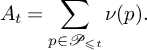 $$ \begin{align} A_t = \sum_{p \in \mathcal{P}_{\leqslant t}}\nu(p). \end{align} $$
Then
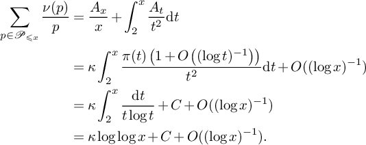 $$ \begin{align} \sum_{p \in \mathcal{P}_{\leqslant x}}\frac{\nu(p)}{p}&=\frac{A_x}{x} + \int_{2}^x \frac{A_t}{t^2}\textrm{d}t\nonumber\\ &=\kappa\int_{2}^x \frac{\pi(t)\left(1+O\left((\log t)^{-1}\right)\right)}{t^2} \textrm{d}t + O((\log x)^{-1})\nonumber\\ &=\kappa\int_{2}^x \frac{\textrm{d}t}{t\log t} + C+O((\log x)^{-1})\nonumber\\ &=\kappa\log\log x + C + O((\log x)^{-1}). \end{align} $$
We deduce (4.10) by taking the exponential of (4.16).
We can prove (4.11) in a similar way. When $i=0$
and
$i=0$
and $f_0 \not \equiv 1$
, we have
$f_0 \not \equiv 1$
, we have $\varrho _0(p) = p$
, and so the result is a consequence of Mertens’ theorem [Reference Iwaniec and Kowalski29, Equation (2.16)]. For any
$\varrho _0(p) = p$
, and so the result is a consequence of Mertens’ theorem [Reference Iwaniec and Kowalski29, Equation (2.16)]. For any $i\in \{1,\ldots , k\}$
, we have
$i\in \{1,\ldots , k\}$
, we have
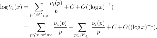 $$ \begin{align} \log V_i(x)&=\sum_{p\in \mathcal{P'}_{\leqslant x}}\frac{\nu_i(p)}{p} + C + O((\log x)^{-1})\nonumber\\ &=\sum_{p\leqslant x \textrm{ prime}}\frac{\nu_i(p)}{p} - \sum_{p\in \mathcal{P}_{\leqslant x}}\frac{\nu_i(p)}{p} + C + O((\log x)^{-1}). \end{align} $$
Similarly to above, using partial summation and (2.5), we have
 $$ \begin{align}\sum_{p\in \mathcal{P}_{\leqslant x}}\frac{\nu_i(p)}{p} = \alpha\theta_i \log\log x + C+ O((\log x)^{-1}).\end{align} $$
To treat the first sum in (4.17), we define $L_i$
to be the number field generated by
$L_i$
to be the number field generated by $f_i$
. For all but finitely many primes p, the quantity
$f_i$
. For all but finitely many primes p, the quantity $\nu _i(p)$
is equal to the number of degree one prime ideals
$\nu _i(p)$
is equal to the number of degree one prime ideals $\mathfrak {p}$
in
$\mathfrak {p}$
in $L_i$
above p. Let
$L_i$
above p. Let $\pi _{L_i}(x)$
denote the number of prime ideals
$\pi _{L_i}(x)$
denote the number of prime ideals $\mathfrak {p}$
in L of norm at most x. This count is dominated by degree one ideals. In fact, the number of prime ideals of degree at least
$\mathfrak {p}$
in L of norm at most x. This count is dominated by degree one ideals. In fact, the number of prime ideals of degree at least $2$
enumerated by
$2$
enumerated by $\pi _{L_i}(x)$
is
$\pi _{L_i}(x)$
is $O(x^{1/2})$
because such an ideal must lie over a rational prime
$O(x^{1/2})$
because such an ideal must lie over a rational prime $p \leqslant x^{1/2}$
and each rational prime p has at most
$p \leqslant x^{1/2}$
and each rational prime p has at most $[L_i:\mathbb {Q}]$
prime ideals in
$[L_i:\mathbb {Q}]$
prime ideals in $L_i$
lying above it. Therefore,
$L_i$
lying above it. Therefore,
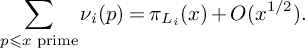 $$ \begin{align*}\sum_{p\leqslant x \textrm{ prime}}\nu_i(p) = \pi_{L_i}(x) + O(x^{1/2}).\end{align*} $$
Using partial summation, as above, together with the Prime ideal theorem [Reference Mitsui38], we deduce that
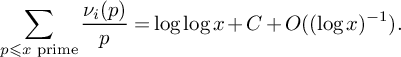 $$ \begin{align} \sum_{p\leqslant x \textrm{ prime}}\frac{\nu_i(p)}{p} = \log\log x + C + O((\log x)^{-1}). \end{align} $$
Combining this with (4.18) and taking exponentials, we deduce the asymptotic in (4.11).
In the following lemma, we record three more useful estimates following similar arguments to Lemma 4.3.
Lemma 4.4. There exists constants $C,C_i>0$
such that
$C,C_i>0$
such that
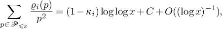 $$ \begin{align} \sum_{p \in \mathcal{P}_{\leqslant x}} \frac{\varrho _i(p)}{p^2} &=(1-\kappa_i)\log\log x + C + O((\log x)^{-1}), \end{align} $$
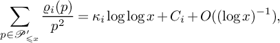 $$ \begin{align} \sum_{p \in \mathcal{P}^{\prime}_{\leqslant x}} \frac{\varrho _i(p)}{p^2} &=\kappa_i\log\log x + C_i + O((\log x)^{-1}), \qquad\end{align} $$
 $$ \begin{align} \sum_{p \in \mathcal{P}^{\prime}_{\leqslant x}} \frac{\varrho _i(p)}{p^2}\log p &=\kappa_i\log x +O(1). \qquad\qquad\qquad \qquad\qquad\end{align} $$
Proof. The estimates (4.20) and (4.21) are immediate consequences of (4.16), (4.18) and (4.19), together with fact that
 $$ \begin{align*}\frac{\varrho _i(p)}{p^2} =\frac{(p-1)\nu_i(p)+1}{p^2}= \frac{\nu_i(p)}{p} + O(p^{-2}).\end{align*} $$
To prove (4.22), we proceed via partial summation in a very similar manner to (4.16). We recall from the Prime number theorem that
 $$ \begin{align} \pi(t) = \frac{t}{\log t}+\frac{t}{(\log t)^2} + O\left(\frac{t}{(\log t)^3}\right). \end{align} $$
For $A_t$
as defined in (4.15), we have
$A_t$
as defined in (4.15), we have
 $$ \begin{align*} \sum_{p \in \mathcal{P}^{\prime}_{\leqslant x}}\frac{\varrho _i(p)}{p^2}\log p &= \sum_{p \in \mathcal{P}^{\prime}_{\leqslant x}}\frac{\nu_i(p)}{p}\log p + O(1)\\ &=\frac{A_x\log x}{x} - \int_{2}^x A_t\left(\frac{\log t}{t}\right)' \textrm{d}t + O(1)\\ &=\kappa_i\int_2^x \frac{(\log t -1)\pi(t)(1+O((\log t)^{-A})}{t^2} \textrm{d}t + O(1)\\ &=\kappa_i\int_{2}^x \frac{1}{t} + O\left(\frac{1}{t(\log t)^{2}}\right) \textrm{d}t + O(1) \quad (\textrm{from } (4.3))\\ &=\kappa_i\log x + O(1), \end{align*} $$
as required.
4.3 The sum
$S_1$

We apply the lower bound sieve $\Lambda ^{-}(\mathcal {A}, \mathcal {P}, g, N^{\gamma })$
and the level of distribution result from Corollary 3.2 with
$\Lambda ^{-}(\mathcal {A}, \mathcal {P}, g, N^{\gamma })$
and the level of distribution result from Corollary 3.2 with $g_1(x,y)=1, g_2(x,y)=f(x,y), D_1=1$
and
$g_1(x,y)=1, g_2(x,y)=f(x,y), D_1=1$
and $D_2= N^{\gamma }$
. The hypotheses of Corollary 3.2 require that
$D_2= N^{\gamma }$
. The hypotheses of Corollary 3.2 require that $\gamma <1$
. We obtain
$\gamma <1$
. We obtain
 $$ \begin{align} S_1 \geqslant (B+o(1))XV(N^{\gamma}). \end{align} $$
By Lemma 4.3, we have
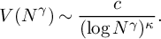 $$ \begin{align*}V(N^{\gamma})\sim \frac{c}{(\log N^{\gamma})^{\kappa}}.\end{align*} $$
For any $\epsilon>0$
, taking
$\epsilon>0$
, taking $\gamma $
sufficiently close to
$\gamma $
sufficiently close to $1$
, we obtain
$1$
, we obtain
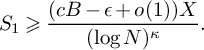 $$ \begin{align} S_1 \geqslant \frac{(cB-\epsilon+o(1))X}{(\log N)^{\kappa}}. \end{align} $$
4.4 The sums
$S_2^{(i)}$

We write $f_i(a,b) = pr$
, for
$f_i(a,b) = pr$
, for $p \in \mathcal {P}$
and
$p \in \mathcal {P}$
and $N^{\gamma }< p \ll N$
. We apply the switching principle, which transforms the sum over p defining
$N^{\gamma }< p \ll N$
. We apply the switching principle, which transforms the sum over p defining $S_2^{(i)}$
into a much shorter sum over the variable r.
$S_2^{(i)}$
into a much shorter sum over the variable r.
Let $R=N^{1-\gamma }$
. The sums
$R=N^{1-\gamma }$
. The sums $S_2^{(i)}$
only involve linear factors
$S_2^{(i)}$
only involve linear factors $f_i(x,y)$
since we assume
$f_i(x,y)$
since we assume $i\in \{0,\ldots , m\}$
. Therefore, for
$i\in \{0,\ldots , m\}$
. Therefore, for $(a,b) \in \mathcal {R}\cap \mathbb {Z}^2$
, we have
$(a,b) \in \mathcal {R}\cap \mathbb {Z}^2$
, we have $f_i(a,b) \ll N$
, and so
$f_i(a,b) \ll N$
, and so $|r|\ll R$
. Let
$|r|\ll R$
. Let $z = N^{1/3}$
. We shall take
$z = N^{1/3}$
. We shall take $\gamma $
arbitrarily close to 1; for now, we assume that
$\gamma $
arbitrarily close to 1; for now, we assume that $\gamma>2/3$
. Then by definition of
$\gamma>2/3$
. Then by definition of $S(\mathcal {A}_p^{(i)},\mathcal {P},p)$
, we know that
$S(\mathcal {A}_p^{(i)},\mathcal {P},p)$
, we know that $\gcd (r, P(R))=1$
and
$\gcd (r, P(R))=1$
and $\gcd (f(a,b),P(z))=1$
.
$\gcd (f(a,b),P(z))=1$
.
Let $r' = |r|/\gcd (r,\Delta )$
. We now explain why
$r' = |r|/\gcd (r,\Delta )$
. We now explain why $r'$
only has prime factors in
$r'$
only has prime factors in $\mathcal {P}'$
. Fix
$\mathcal {P}'$
. Fix $l \in S$
. Recall the assumption that
$l \in S$
. Recall the assumption that $\nu _l(f(a_0,b_0)) < \nu _l(\Delta )$
. Since
$\nu _l(f(a_0,b_0)) < \nu _l(\Delta )$
. Since $f_i(a_0,b_0) \mid f(a_0,b_0)$
and
$f_i(a_0,b_0) \mid f(a_0,b_0)$
and $f_i(a,b) \equiv f_i(a_0,b_0) \ (\mathrm {mod}\ \Delta )$
(by the condition
$f_i(a,b) \equiv f_i(a_0,b_0) \ (\mathrm {mod}\ \Delta )$
(by the condition $C(a,b)$
), we have
$C(a,b)$
), we have
 $$ \begin{align} \nu_l(r) = \nu_l(f_i(a, b)) \leqslant \nu_l(f(a,b)) = \nu_l(f(a_0,b_0)) < \nu_l(\Delta). \end{align} $$
Therefore, $\gcd (r',\Delta ) =1$
, and by the assumption that every prime in S divides
$\gcd (r',\Delta ) =1$
, and by the assumption that every prime in S divides $\Delta $
, this implies
$\Delta $
, this implies $r'$
has no prime factors in S. Moreover, p is the smallest prime in
$r'$
has no prime factors in S. Moreover, p is the smallest prime in $\mathcal {P}$
dividing
$\mathcal {P}$
dividing $f_i(a,b)$
. Since
$f_i(a,b)$
. Since $r<p$
, this means that
$r<p$
, this means that $r'$
has no prime factors in
$r'$
has no prime factors in $\mathcal {P}$
, and hence only has prime factors in
$\mathcal {P}$
, and hence only has prime factors in $\mathcal {P}'$
.
$\mathcal {P}'$
.
However, $f_i(a,b)/r'$
has no prime factors in
$f_i(a,b)/r'$
has no prime factors in $\mathcal {P}'$
. Therefore,
$\mathcal {P}'$
. Therefore,
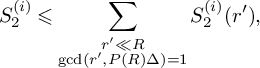 $$ \begin{align} S_2^{(i)} \leqslant \sum_{\substack{r'\ll R\\ \gcd(r',P(R)\Delta)=1}}S_2^{(i)}(r'), \end{align} $$
where
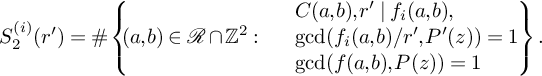 $$ \begin{align} S_2^{(i)}(r') = \#\left\{\!\!\!(a,b) \in \mathcal{R}\cap \mathbb{Z}^2: \begin{array}{l l l} &\displaystyle C(a,b), r'\mid f_i(a,b), \\ &\displaystyle \gcd(f_i(a,b)/r', P'(z))=1\\ &\displaystyle \gcd(f(a,b),P(z))=1 \end{array} \!\!\!\!\!\right\}. \end{align} $$
Below, for convenience, we change notation from $r'$
back to r.
$r'$
back to r.
Let $\Lambda _1^+, \Lambda _2^+$
be upper bound sieves of level z. Defining
$\Lambda _1^+, \Lambda _2^+$
be upper bound sieves of level z. Defining $A(dr,e), r(dr,e)$
as in Section 3 with
$A(dr,e), r(dr,e)$
as in Section 3 with $g_1(x,y) = f_i(x,y)$
and
$g_1(x,y) = f_i(x,y)$
and $g_2(x,y) = f(x,y)$
, and writing
$g_2(x,y) = f(x,y)$
, and writing
 $$\begin{align*}m_1 = \gcd\left(\frac{f_i(a,b)}{r}, P'(z)\right), \qquad m_2= \gcd(f(a,b), P(z)), \end{align*}$$
we obtain
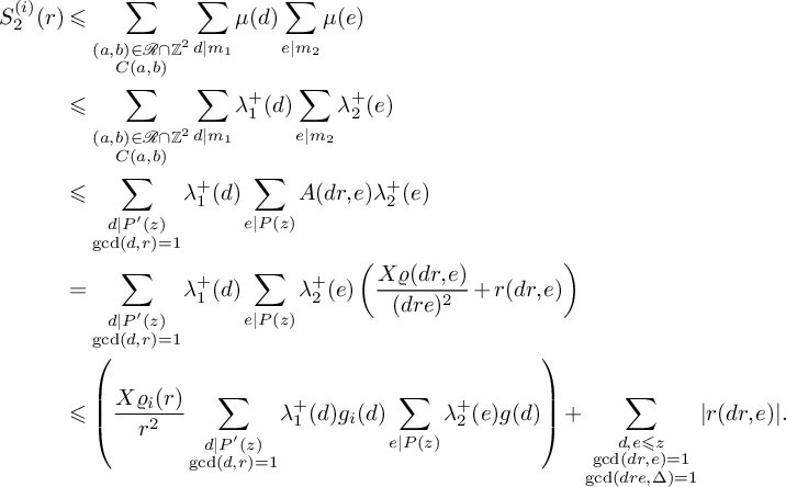 $$ \begin{align} S_2^{(i)}(r) &\leqslant \sum_{\substack{(a,b) \in \mathcal{R}\cap \mathbb{Z}^2\\ C(a,b)}}\sum_{d \mid m_1}\mu(d)\sum_{e\mid m_2}\mu(e)\nonumber\\ &\leqslant \sum_{\substack{(a,b) \in \mathcal{R}\cap \mathbb{Z}^2\\ C(a,b)}}\sum_{d \mid m_1}\lambda_1^+(d)\sum_{e\mid m_2}\lambda_2^+(e)\nonumber\\ &\leqslant \sum_{\substack{d \mid P'(z)\\ \gcd(d,r)=1}}\lambda_1^+(d)\sum_{e\mid P(z)}A(dr,e)\lambda_2^+(e)\nonumber\\ &=\sum_{\substack{d \mid P'(z)\\ \gcd(d,r)=1}}\lambda_1^+(d)\sum_{e\mid P(z)}\lambda_2^+(e)\left(\frac{X\varrho (dr,e)}{(dre)^2} + r(dr,e)\right)\nonumber\\ &\leqslant \left(\frac{X\varrho _i(r)}{r^2}\sum_{\substack{d \mid P'(z)\\ \gcd(d,r) = 1}}\lambda_1^+(d)g_i(d)\sum_{\substack{e \mid P(z)}}\lambda_2^+(e)g(d)\right) + \sum_{\substack{d,e \leqslant z\\ \gcd(dr,e) = 1\\ \gcd(dre, \Delta) = 1}}|r(dr,e)|. \end{align} $$
Choose $\lambda _1^+,\lambda _2^+$
to be the beta sieves
$\lambda _1^+,\lambda _2^+$
to be the beta sieves $\Lambda ^+(\mathcal {P}'\backslash \{p\mid r\}, g_i, N^{1/3}), \Lambda ^+(\mathcal {P}, g, N^{1/3})$
, respectively. Then the remainder term in (4.29) can be bounded by
$\Lambda ^+(\mathcal {P}'\backslash \{p\mid r\}, g_i, N^{1/3}), \Lambda ^+(\mathcal {P}, g, N^{1/3})$
, respectively. Then the remainder term in (4.29) can be bounded by
 $$ \begin{align*}\sum_{\substack{d,e \leqslant N^{1/3}\\ \gcd(dr,e) = 1\\ \gcd(dre, \Delta) = 1}}|r(dr,e)| \leqslant \sum_{\substack{d \ll N^{1/3}R\\e \ll N^{1/3}\\ \gcd(dr,e) = 1\\ \gcd(dre, \Delta) = 1}}|r(d,e)|,\end{align*} $$
which is negligible by Lemma 3.6 because $N^{2/3}R = N^{5/3-\gamma } \ll N^{1-\epsilon }$
.
$N^{2/3}R = N^{5/3-\gamma } \ll N^{1-\epsilon }$
.
Define a multiplicative function $h_i(r)$
supported on squarefree integers r, which is zero unless all prime factors of r are in
$h_i(r)$
supported on squarefree integers r, which is zero unless all prime factors of r are in $\mathcal {P}'$
and
$\mathcal {P}'$
and
 $$ \begin{align} h_i(r)=\frac{\varrho _i(r)}{r^2}\prod_{p\mid r}\left(1-\frac{\varrho _i(p)}{p^2}\right)^{-1} \end{align} $$
otherwise. Applying Theorem 4.1, we conclude that
 $$ \begin{align*}S_2^{(i)}(r) \leqslant Xh_i(r)V(N^{1/3})V_i(N^{1/3})(AA_i + o(1)).\end{align*} $$
From Lemma 4.3, we obtain
 $$\begin{align*}S_2^{(i)}\leqslant \frac{(cc_iAA_i+o(1))X}{(\log N^{1/3})^{\kappa + \kappa_i}}\sum_{\substack{r \ll R}}h_i(r). \end{align*}$$
To deal with the sum over $h_i(r)$
, we note that
$h_i(r)$
, we note that
 $$ \begin{align} \sum_{\substack{r \ll R}}h_i(r) \leqslant \prod_{\substack{p \in \mathcal{P}'\\p\ll R}}\left(1+\sum_{m=1}^{\infty} h_i(p^m)\right)= \prod_{\substack{p \in \mathcal{P}'\\p \ll R}}\left(1-g_i(p)\right)^{-1}(1+O(p^{-2})). \end{align} $$
Applying Lemma 4.3 to the product, we obtain
 $$ \begin{align*}\sum_{\substack{r \ll R}}h_i(r) \ll (\log R)^{\kappa_i}.\end{align*} $$
Since $R=N^{1-\gamma }$
, we deduce that
$R=N^{1-\gamma }$
, we deduce that
 $$ \begin{align*}S_2^{(i)} \ll \frac{cc_iAA_iX}{(\log N)^{\kappa}}\left(\frac{(1-\gamma)^{\kappa_i}}{(1/3)^{\kappa_i+\kappa}}\right).\end{align*} $$
Therefore, $S_2^{(i)}$
can be made negligible compared to
$S_2^{(i)}$
can be made negligible compared to $S_1$
by taking
$S_1$
by taking $\gamma $
arbitrarily close to 1.
$\gamma $
arbitrarily close to 1.
4.5 The sums
$S_3^{(i)}$

For a fixed prime p and an upper bound sieve $\lambda ^+$
of level z, we have
$\lambda ^+$
of level z, we have
 $$ \begin{align*}S(\mathcal{A}_p^{(i)},\mathcal{P}, z) \leqslant \sum_{d\mid P(z)}\lambda^+(d)A(p,d),\end{align*} $$
where $A(p,d)$
is as in Section 3 with
$A(p,d)$
is as in Section 3 with $g_1(x,y) = f_i(x,y)$
and
$g_1(x,y) = f_i(x,y)$
and $g_2(x,y) = f(x,y)$
.
$g_2(x,y) = f(x,y)$
.
We first deal with the primes p in the interval $I:=(N^{\gamma }, N^{2-\gamma -\epsilon }]$
. For any
$I:=(N^{\gamma }, N^{2-\gamma -\epsilon }]$
. For any $p\in I$
, let
$p\in I$
, let $\lambda ^+$
be the beta sieve
$\lambda ^+$
be the beta sieve $\Lambda ^+(\mathcal {A}_p^{(i)}, \mathcal {P}, g_i(p)g, N^{\gamma })$
. We obtain
$\Lambda ^+(\mathcal {A}_p^{(i)}, \mathcal {P}, g_i(p)g, N^{\gamma })$
. We obtain
 $$ \begin{align} S(\mathcal{A}_p^{(i)}, \mathcal{P},p) &\leqslant S(\mathcal{A}_p^{(i)}, \mathcal{P},N^{\gamma})\nonumber\\ &\leqslant (A+o(1))XV(N^{\gamma})g_i(p) + \sum_{\substack{d \leqslant N^{\gamma}\\ \gcd(d,p\Delta)=1}}|r(p,N^{\gamma})|. \end{align} $$
We apply Corollary 3.2 with $D_1 = N^{2-\gamma - \epsilon }$
and
$D_1 = N^{2-\gamma - \epsilon }$
and $D_2 = N^{\gamma }$
. These choices of
$D_2 = N^{\gamma }$
. These choices of $D_1,D_2$
satisfy the hypotheses of Corollary 3.2. Taking a sum over
$D_1,D_2$
satisfy the hypotheses of Corollary 3.2. Taking a sum over $p\in I$
, the contribution from the remainder term in (4.32) is negligible. We obtain
$p\in I$
, the contribution from the remainder term in (4.32) is negligible. We obtain
 $$ \begin{align} \sum_{\substack{p \in I\cap \mathcal{P}}}S(\mathcal{A}_p^{(i)}, \mathcal{P},p)\leqslant (A+o(1)) XV(N^{\gamma})\sum_{p \in I\cap \mathcal{P}}g_i(p). \end{align} $$
It follows from Lemma 4.4 that
 $$ \begin{align*} \sum_{\substack{N^{\gamma}<p\leqslant N^{2-\gamma-\epsilon}}}g_i(p) &= \log\log N^{2-\gamma-\epsilon} - \log\log N^{\gamma} + o(1)\\ &= \log(2-\gamma - \epsilon) - \log \gamma +o(1). \end{align*} $$
Therefore, the contribution to $S_3^{(i)}$
from this range is negligible if we take
$S_3^{(i)}$
from this range is negligible if we take $\gamma $
arbitrarily close to 1.
$\gamma $
arbitrarily close to 1.
In the remaining range $N^{2-\gamma -\epsilon }< p <N^{\beta _i}$
, we split into dyadic intervals
$N^{2-\gamma -\epsilon }< p <N^{\beta _i}$
, we split into dyadic intervals $(R,2R]$
. Note that for
$(R,2R]$
. Note that for $p\in (R,2R]$
, the assumption
$p\in (R,2R]$
, the assumption $\gamma <1$
implies that
$\gamma <1$
implies that $N^{2-\epsilon }/R <p$
, so
$N^{2-\epsilon }/R <p$
, so $S(\mathcal {A}_p^{(i)}, \mathcal {P}, p) \leqslant S(\mathcal {A}_p^{(i)}, \mathcal {P}, N^{2-\epsilon }/R)$
. For each dyadic interval, we apply the beta sieve
$S(\mathcal {A}_p^{(i)}, \mathcal {P}, p) \leqslant S(\mathcal {A}_p^{(i)}, \mathcal {P}, N^{2-\epsilon }/R)$
. For each dyadic interval, we apply the beta sieve $\Lambda ^+(\mathcal {A}_p^{(i)}, \mathcal {P}, g_i(p)g, N^{2-\epsilon }/R)$
and the level of distribution result from Corollary 3.2 with
$\Lambda ^+(\mathcal {A}_p^{(i)}, \mathcal {P}, g_i(p)g, N^{2-\epsilon }/R)$
and the level of distribution result from Corollary 3.2 with $D_1=2R$
and
$D_1=2R$
and $D_2 = N^{2-\epsilon }/R$
. At this point, we need to assume that
$D_2 = N^{2-\epsilon }/R$
. At this point, we need to assume that $\beta _i<2$
for all i, so that
$\beta _i<2$
for all i, so that $D_2\geqslant 1$
. We obtain
$D_2\geqslant 1$
. We obtain
 $$ \begin{align} &\sum_{\substack{N^{2-\gamma-\epsilon}<p< N^{\beta_i}\\ p \in \mathcal{P}}}S(\mathcal{A}_p^{(i)}, \mathcal{P},p) \end{align} $$
 $$ \begin{align} &\leqslant \sum_{\substack{R \textrm{ dyadic}\\N^{2-\gamma -\epsilon}<R < N^{\beta_i}}}\sum_{\substack{p \in (R,2R]\\ p \in \mathcal{P}}}S(\mathcal{A}_p^{(i)}, \mathcal{P},N^{2-\epsilon}/R)\nonumber\\ &\leqslant (A+o(1))X\sum_{\substack{R \textrm{ dyadic}\\ N^{2-\gamma -\epsilon}<R < N^{\beta_i}}}V(N^{2-\epsilon}/R)\sum_{\substack{p \in (R,2R]\\p \in \mathcal{P}}}g_i(p)\nonumber\\ &\leqslant \frac{(cA+o(1))X}{(\log N)^{\kappa}}\sum_{\substack{ N^{2-\gamma-\epsilon} \leqslant p< N^{\beta_i}\\p \in \mathcal{P}}}\frac{g_i(p)}{(2-\epsilon - \frac{\log p}{\log N})^{\kappa}}, \end{align} $$
where the last line follows from Lemma 4.3 and the fact that $V(N^{2-\epsilon }/R)<V(N^{2-\epsilon -\log p/\log N})$
for all
$V(N^{2-\epsilon }/R)<V(N^{2-\epsilon -\log p/\log N})$
for all $p\in (R,2R]$
.
$p\in (R,2R]$
.
We denote the sum in (4.35) by $T(\beta _i, \kappa )$
. Since
$T(\beta _i, \kappa )$
. Since $\gamma <1$
, we have
$\gamma <1$
, we have $2-\gamma -\epsilon>1$
for sufficiently small
$2-\gamma -\epsilon>1$
for sufficiently small $\epsilon $
, and so we may upper bound
$\epsilon $
, and so we may upper bound $T(\beta _i,\kappa )$
by enlarging its range of summation to
$T(\beta _i,\kappa )$
by enlarging its range of summation to $N<p< N^{\beta _i}$
. Define
$N<p< N^{\beta _i}$
. Define
 $$ \begin{align*}A(t) = \sum_{p \in \mathcal{P}_{\leqslant t}}g_i(p), \qquad h(t) = \left(2-\epsilon - \frac{\log t}{\log N}\right)^{-\kappa}.\end{align*} $$
From Lemma 4.4, we have $A(t)= (1-\kappa _i)\log \log t + C+o(1)$
for some constant C. In particular, for any
$A(t)= (1-\kappa _i)\log \log t + C+o(1)$
for some constant C. In particular, for any $r>0$
, we have
$r>0$
, we have $A(N^r)-A(N) = (1-\kappa _i)\log r + o(1)$
. Applying summation by parts, followed by the substitution
$A(N^r)-A(N) = (1-\kappa _i)\log r + o(1)$
. Applying summation by parts, followed by the substitution $t=N^s$
, we obtain
$t=N^s$
, we obtain
 $$ \begin{align} T(\beta_i,\kappa) &\leqslant (A(N^{\beta_i})-A(N))h(N^{\beta_i}) - \int_{N}^{N^{\beta_i}}(A(t)-A(N))h'(t) \textrm{d}t \nonumber \\ & =(A(N^{\beta_i})-A(N))h(N^{\beta_i}) - \int_{1}^{\beta_i}(A(N^s)-A(N))\frac{\partial h(N^s)}{\partial s}\textrm{d}s \nonumber \\ &=(1-\kappa_i)\log \beta_i h(N^{\beta_i}) -(1-\kappa_i)\int_{1}^{\beta_i}(\log s) \frac{\partial h(N^s)}{\partial s}\textrm{d}s + o(1) \nonumber \\ &=(1-\kappa_i)\int_{1}^{\beta_i}\frac{h(N^s)}{s}\textrm{d}s + o(1). \end{align} $$
Taking $\epsilon $
sufficiently small and redefining it appropriately, we may replace
$\epsilon $
sufficiently small and redefining it appropriately, we may replace $h(N^s)$
by
$h(N^s)$
by $(2-s)^{-\kappa }$
at the cost of adding
$(2-s)^{-\kappa }$
at the cost of adding $\epsilon $
in (4.36). Combining with (4.35), we conclude that for any
$\epsilon $
in (4.36). Combining with (4.35), we conclude that for any $\epsilon>0$
,
$\epsilon>0$
,
 $$ \begin{align} S_3^{(i)}\leqslant \frac{(cA+\epsilon+o(1))X}{(\log N)^{\kappa}}\cdot (1-\kappa_i) \int_{1}^{\beta_i}(2-s)^{-\kappa}\frac{\textrm{d}s}{s}. \end{align} $$
Due to the factor $1-\kappa _i = \alpha \theta _i$
appearing in the above estimate,
$1-\kappa _i = \alpha \theta _i$
appearing in the above estimate, $S_3^{(i)}$
becomes negligible compared to
$S_3^{(i)}$
becomes negligible compared to $S_1$
as
$S_1$
as $\alpha \rightarrow 0$
. We perform a more precise quantitative comparison in Section 4.7.
$\alpha \rightarrow 0$
. We perform a more precise quantitative comparison in Section 4.7.
4.6 The sums
$S_4^{(i)}$

We begin in a similar manner to the sums $S_2^{(i)}$
, by writing
$S_2^{(i)}$
, by writing $f_i(a,b) = pr$
, for
$f_i(a,b) = pr$
, for $p \in \mathcal {P}$
, where now
$p \in \mathcal {P}$
, where now $N^{\beta _i}\leqslant p < x$
and
$N^{\beta _i}\leqslant p < x$
and $R=x/N^{\beta _i}$
. Let
$R=x/N^{\beta _i}$
. Let $D_1 = N^{\eta _1}$
and
$D_1 = N^{\eta _1}$
and $D_2 = N^{\eta _2}$
for parameters
$D_2 = N^{\eta _2}$
for parameters $\eta _1, \eta _2>0$
(which may depend on r and i) to be chosen later. We assume
$\eta _1, \eta _2>0$
(which may depend on r and i) to be chosen later. We assume $\eta _2 < \beta _i$
so that the condition
$\eta _2 < \beta _i$
so that the condition $\gcd (f(a,b), P(p)) =1$
can be replaced by the weaker condition
$\gcd (f(a,b), P(p)) =1$
can be replaced by the weaker condition $\gcd (f(a,b), P(N^{\eta _2}))=1$
. Proceeding as in Section 4.4, we have
$\gcd (f(a,b), P(N^{\eta _2}))=1$
. Proceeding as in Section 4.4, we have
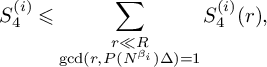 $$ \begin{align} S_4^{(i)} \leqslant \sum_{\substack{r\ll R\\ \gcd(r,P(N^{\beta_i})\Delta)=1}}S_4^{(i)}(r), \end{align} $$
where
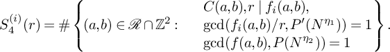 $$ \begin{align} S_4^{(i)}(r) = \#\left\{\!(a,b) \in \mathcal{R}\cap \mathbb{Z}^2: \begin{array}{l l l} &\displaystyle C(a,b), r\mid f_i(a,b), \\ &\displaystyle \gcd(f_i(a,b)/r, P'(N^{\eta_1}))=1\\ &\displaystyle \gcd(f(a,b),P(N^{\eta_2}))=1 \end{array} \!\!\!\!\right\}. \end{align} $$
Similarly to (4.29), for any upper bound sieves $\lambda _1^+, \lambda _2^+$
of levels
$\lambda _1^+, \lambda _2^+$
of levels $N^{\eta _1}, N^{\eta _2}$
, the quantity
$N^{\eta _1}, N^{\eta _2}$
, the quantity $S_4^{(i)}(r)$
is bounded above by
$S_4^{(i)}(r)$
is bounded above by
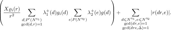 $$\begin{align*}\left(\frac{X\varrho _i(r)}{r^2}\sum_{\substack{d \mid P'(N^{\eta_1})\\ \gcd(d,r) = 1}}\lambda_1^+(d)g_i(d)\sum_{\substack{e \mid P(N^{\eta_2})}}\lambda_2^+(e)g(d)\right) + \sum_{\substack{d\leqslant N^{\eta_1}, e \leqslant N^{\eta_2}\\ \gcd(dr,e) = 1\\ \gcd(dre, \Delta) = 1}}|r(dr,e)|. \end{align*}$$
In order to ensure the error terms from applying the level of distribution result from Corollary 3.2 are negligible after summing over r, we need $\eta _1,\eta _2$
to satisfy
$\eta _1,\eta _2$
to satisfy
 $$ \begin{align} \eta_1, \eta_2>0, \quad \eta_2 \leqslant 1-\delta \qquad (\textrm{for all }r\leqslant R), \end{align} $$
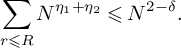 $$ \begin{align} \sum_{r\leqslant R}N^{\eta_1+\eta_2}\leqslant N^{2-\delta}. \end{align} $$
Remark 4.5. There are no $\eta _1,\eta _2$
satisfying (4.40) and (4.41) unless
$\eta _1,\eta _2$
satisfying (4.40) and (4.41) unless $R\leqslant N^{2-\delta }$
, i.e.,
$R\leqslant N^{2-\delta }$
, i.e., $x \leqslant N^{2-\delta + \beta _i}$
. Since we had to assume
$x \leqslant N^{2-\delta + \beta _i}$
. Since we had to assume $\beta _i<2$
in the treatment of the sums
$\beta _i<2$
in the treatment of the sums $S_3^{(i)}$
in Section 4.5, this means our approach cannot handle the case
$S_3^{(i)}$
in Section 4.5, this means our approach cannot handle the case $d \geqslant 4$
, in which
$d \geqslant 4$
, in which $f(x,y)$
has an irreducible factor of degree
$f(x,y)$
has an irreducible factor of degree $\geqslant 4$
. Therefore, we proceed with the additional assumption that
$\geqslant 4$
. Therefore, we proceed with the additional assumption that $d\leqslant 3$
.
$d\leqslant 3$
.
Choose $\lambda ^+_1, \lambda ^+_2$
to be the beta sieves
$\lambda ^+_1, \lambda ^+_2$
to be the beta sieves $\Lambda ^+(\mathcal {P}'\backslash \{p\mid r\}, g_i, N^{\eta _1}), \Lambda ^+(\mathcal {P}, g, N^{\eta _2})$
, respectively. Recalling the definition of
$\Lambda ^+(\mathcal {P}'\backslash \{p\mid r\}, g_i, N^{\eta _1}), \Lambda ^+(\mathcal {P}, g, N^{\eta _2})$
, respectively. Recalling the definition of $h_i(r)$
from (4.30), we obtain
$h_i(r)$
from (4.30), we obtain
 $$ \begin{align} S_4^{(i)}(r) \leqslant (AA_i+o(1))Xh_i(r)V_i(N^{\eta_1})V(N^{\eta_2}).\end{align} $$
Using Lemma 4.3 to estimate the products in (4.42), and taking a sum over r, we obtain
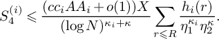 $$ \begin{align} S_4^{(i)}\leqslant \frac{(cc_iAA_i+o(1))X}{(\log N)^{\kappa_i+\kappa}}\sum_{r\leqslant R}\frac{h_i(r)}{\eta_1^{\kappa_i}\eta_2^{\kappa}}. \end{align} $$
We divide the sum over r into dyadic intervals $r \in (R_1,2R_1]$
, and take
$r \in (R_1,2R_1]$
, and take $\eta _1,\eta _2$
depending only on
$\eta _1,\eta _2$
depending only on $R_1$
and i. To obtain a good estimate for (4.43), we maximise
$R_1$
and i. To obtain a good estimate for (4.43), we maximise $\eta _1^{\kappa _i}\eta _2^{\kappa }$
subject to the constraints
$\eta _1^{\kappa _i}\eta _2^{\kappa }$
subject to the constraints
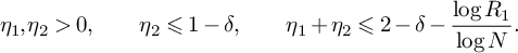 $$ \begin{align*}\eta_1,\eta_2>0, \qquad \eta_2\leqslant 1-\delta, \qquad \eta_1+\eta_2 \leqslant 2-\delta - \frac{\log R_1}{\log N}.\end{align*} $$
By a similar computation to [Reference Irving27, Section 6.5], the optimal solution is
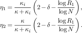 $$ \begin{align*} \eta_1 &= \frac{\kappa_i}{\kappa+\kappa_i}\left(2-\delta-\frac{\log R_1}{\log N}\right),\\ \eta_2 &= \frac{\kappa}{\kappa+\kappa_i}\left(2-\delta-\frac{\log R_1}{\log N}\right). \end{align*} $$
We note that for $\delta>0$
sufficiently small, this solution satisfies
$\delta>0$
sufficiently small, this solution satisfies $\eta _2 \leqslant 1-\delta $
due to the assumption
$\eta _2 \leqslant 1-\delta $
due to the assumption $\kappa <1/2$
. Substituting this choice of
$\kappa <1/2$
. Substituting this choice of $\eta _1,\eta _2$
into (4.43), we obtain
$\eta _1,\eta _2$
into (4.43), we obtain
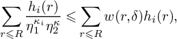 $$ \begin{align} \sum_{r\leqslant R}\frac{h_i(r)}{\eta_1^{\kappa_i}\eta_2^{\kappa}}\leqslant \sum_{r\leqslant R}w(r,\delta)h_i(r), \end{align} $$
where
 $$ \begin{align} w(r,\delta) = \left(\frac{\kappa}{\kappa+\kappa_i}\right)^{-\kappa}\left(\frac{\kappa_i}{\kappa+\kappa_i}\right)^{-\kappa_i}\left(2-\delta -\frac{\log r}{\log N}\right)^{-(\kappa+\kappa_i)}. \end{align} $$
We treat the sum in (4.44) using partial summation, for which we require estimates for $\sum _{r\leqslant t}h_i(r)$
. For the case
$\sum _{r\leqslant t}h_i(r)$
. For the case $d=2$
, the estimate already found in (4.31) is sufficient. Below, we find a more refined estimate which we use in the case
$d=2$
, the estimate already found in (4.31) is sufficient. Below, we find a more refined estimate which we use in the case $d=3$
.
$d=3$
.
We first consider the contribution to (4.44) from squarefree values of r. We would like to apply [Reference Friedlander and Iwaniec18, Theorem A.5], which states that under certain hypothesis on the function $h_i(r)$
, we have
$h_i(r)$
, we have
 $$ \begin{align} \sum_{\substack{m \leqslant x\\ \mu^2(m)=1}}h_i(m)= c_{h_i}(\log x)^{\kappa_i} + O((\log x)^{\kappa_i -1}), \end{align} $$
where
 $$ \begin{align*}c_{h_i} = \frac{1}{\Gamma(\kappa_i+1)}\prod_p \left(1-\frac{1}{p}\right)^{\kappa_i}(1+h_i(p)).\end{align*} $$
In the following lemma, we verify that the function $h_i(r)$
satisfies the required hypotheses for [Reference Friedlander and Iwaniec18, Theorem A.5].
$h_i(r)$
satisfies the required hypotheses for [Reference Friedlander and Iwaniec18, Theorem A.5].
Lemma 4.6. For any $x\geqslant 1$
and any
$x\geqslant 1$
and any $2\leqslant w< z$
, the function
$2\leqslant w< z$
, the function $h_i(r)$
satisfies the following estimates:
$h_i(r)$
satisfies the following estimates:
 $$ \begin{align} \prod_{w\leqslant p <z}(1+h_i(p)) &\ll \left(\frac{\log z}{\log w}\right)^{\kappa_i}, \end{align} $$
 $$ \begin{align} \sum_p h_i(p)^2\log p &< \infty, \end{align} $$
 $$ \begin{align} \sum_{p \leqslant x}h_i(p)\log p &= \kappa_i\log x + O(1). \end{align} $$
Proof. To prove (4.47), we note that $1+h_i(p) = \left (1-\frac {\varrho _i(p)}{p^2}\right )^{-1}$
for all
$1+h_i(p) = \left (1-\frac {\varrho _i(p)}{p^2}\right )^{-1}$
for all $p\in \mathcal {P}'$
. The result is then immediate from Lemma 4.3. To prove (4.45), we recall that
$p\in \mathcal {P}'$
. The result is then immediate from Lemma 4.3. To prove (4.45), we recall that $\varrho _i(p) \ll p$
, and so
$\varrho _i(p) \ll p$
, and so $h_i(p) \ll p^{-1}$
. Therefore,
$h_i(p) \ll p^{-1}$
. Therefore,
 $$ \begin{align*}\sum_{p}h_i(p)^2\log p \ll \sum_{p}\frac{\log p}{p^2}< \infty.\end{align*} $$
Finally, we note that
 $$ \begin{align*} \sum_{p\leqslant x}h_i(p)\log p =\sum_{p \in \mathcal{P}^{\prime}_{\leqslant x}}\frac{\varrho _i(p)}{p^2}\log p + O(1), \end{align*} $$
We can now evaluate the sum in (4.44) using partial summation. We obtain
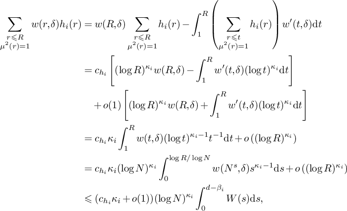 $$ \begin{align*} \sum_{\substack{r\leqslant R\\ \mu^2(r) = 1}}w(r,\delta)h_i(r)&= w(R,\delta)\sum_{\substack{r\leqslant R\\ \mu^2(r)=1}}h_i(r)-\int_{1}^R \left(\sum_{\substack{r\leqslant t\\ \mu^2(r)=1}}h_i(r)\right)w'(t,\delta) \textrm{d}t\\ &=c_{h_i}\left[(\log R)^{\kappa_i}w(R,\delta)-\int_{1}^R w'(t,\delta)(\log t)^{\kappa_i}\textrm{d}t\right]\\ &\quad +o(1)\left[(\log R)^{\kappa_i}w(R,\delta)+\int_{1}^R w'(t,\delta)(\log t)^{\kappa_i}\textrm{d}t\right]\\ &= c_{h_i}\kappa_i\int_{1}^R w(t,\delta)(\log t)^{\kappa_i-1}t^{-1}\textrm{d}t+o\left((\log R)^{\kappa_i}\right)\\ &=c_{h_i}\kappa_i(\log N)^{\kappa_i}\int_{0}^{\log R/\log N}w(N^s, \delta)s^{\kappa_i -1}\textrm{d}s + o\left((\log R)^{\kappa_i}\right)\\ &\leqslant (c_{h_i}\kappa_i +o(1))(\log N)^{\kappa_i}\int_{0}^{d-\beta_i}W(s)\textrm{d}s, \end{align*} $$
where $W(s) = w(N^s, 0)s^{\kappa _i-1}.$
We now consider the contribution to (4.30) from those r which are not squarefree. Let $d_i$
denote the degree of
$d_i$
denote the degree of $f_i$
. From [Reference Daniel15, Lemma 3.1], we have
$f_i$
. From [Reference Daniel15, Lemma 3.1], we have $\varrho _i(p^{\alpha }) \ll p^{2\alpha (1-1/d_i)}$
for all primes
$\varrho _i(p^{\alpha }) \ll p^{2\alpha (1-1/d_i)}$
for all primes $p \notin S$
and any positive integer
$p \notin S$
and any positive integer $\alpha $
. By the multiplicativity of
$\alpha $
. By the multiplicativity of $h_i(r)$
, it follows that
$h_i(r)$
, it follows that $h_i(r) \ll r^{-2/d_i +\epsilon }$
.
$h_i(r) \ll r^{-2/d_i +\epsilon }$
.
We recall that a positive integer n is squareful if for any prime $p\mid n$
, we also have
$p\mid n$
, we also have $p^2\mid n$
. Since
$p^2\mid n$
. Since $d_i\leqslant 3$
, we have
$d_i\leqslant 3$
, we have
 $$ \begin{align*}\sum_{r \textrm{ squareful}}h_i(r) \ll \sum_{r \textrm{ squareful}}r^{-2/d_i + \epsilon} \leqslant \sum_{r \textrm{ squareful}}r^{-2/3 + \epsilon}< \infty,\end{align*} $$
where the last inequality follows from partial summation together with the fact that there are $O(M^{1/2})$
squareful positive integers less than M. Since
$O(M^{1/2})$
squareful positive integers less than M. Since $h_i(r)$
is supported on integers with no prime factors in S, for any
$h_i(r)$
is supported on integers with no prime factors in S, for any $\epsilon>0$
, there exists a set of primes
$\epsilon>0$
, there exists a set of primes $S_0$
, depending only on
$S_0$
, depending only on $\epsilon $
and f, such that for any
$\epsilon $
and f, such that for any $S\supseteq S_0$
, we have
$S\supseteq S_0$
, we have
 $$ \begin{align*}\sum_{\substack{r \textrm{ squareful}\\ r>1}}h_i(r) <\epsilon.\end{align*} $$
For the remainder of this section, we assume that $S\supseteq S_0$
. Proceeding as in [Reference Irving27, Lemma 6.2], we use that
$S\supseteq S_0$
. Proceeding as in [Reference Irving27, Lemma 6.2], we use that $w(r,\delta ) \ll 1$
, and decompose each non-squarefree r into
$w(r,\delta ) \ll 1$
, and decompose each non-squarefree r into $r=r_1r_2$
, where
$r=r_1r_2$
, where $r_1$
is squarefree and
$r_1$
is squarefree and $r_2>1$
is squareful. We have
$r_2>1$
is squareful. We have
 $$ \begin{align*}\sum_{\substack{r \leqslant R\\ \mu^2(r)=0}}w(r,\delta)h_i(r) \ll \sum_{\substack{r_1 \leqslant R\\ \mu^2(r_1)=1}}h_i(r_1) \sum_{\substack{r_2 \textrm{ squareful}\\right_2>1}}h_i(r_2).\end{align*} $$
Combining with (4.46), we deduce that for any $\epsilon>0$
, we have
$\epsilon>0$
, we have
 $$ \begin{align*}\sum_{\substack{r \leqslant R\\ \mu^2(r)=0}}w(r,\delta)h_i(r) \leqslant (\epsilon + o(1))(\log N)^{\kappa_i}.\end{align*} $$
In conclusion, we have the upper bound
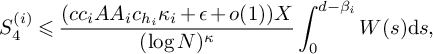 $$ \begin{align} S_4^{(i)} \leqslant \frac{(cc_iAA_ic_{h_i}\kappa_i + \epsilon + o(1))X}{(\log N)^{\kappa}}\int_{0}^{d-\beta_i}W(s)\textrm{d}s, \end{align} $$
where
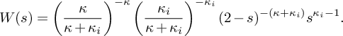 $$ \begin{align} W(s)= \left(\frac{\kappa}{\kappa+\kappa_i}\right)^{-\kappa}\left(\frac{\kappa_i}{\kappa+\kappa_i}\right)^{-\kappa_i}(2-s)^{-(\kappa+\kappa_i)}s^{\kappa_i-1}. \end{align} $$
Remark 4.7. Whilst $c,c_i, c_{h_i}$
all depend on S, the ratio
$c,c_i, c_{h_i}$
all depend on S, the ratio $\kappa _ic_ic_{h_i}AA_i/B$
of the constants in the bounds for
$\kappa _ic_ic_{h_i}AA_i/B$
of the constants in the bounds for $S_4^{(i)}$
and
$S_4^{(i)}$
and $S_1$
is independent of S, as seen below in (4.52). Therefore, we may indeed take
$S_1$
is independent of S, as seen below in (4.52). Therefore, we may indeed take $\epsilon $
to be arbitrarily small in (4.50) without sacrificing anything in our comparison of
$\epsilon $
to be arbitrarily small in (4.50) without sacrificing anything in our comparison of $S_1$
and
$S_1$
and $S_4^{(i)}$
. The
$S_4^{(i)}$
. The $o(1)$
terms in (4.50) and in the bounds for the other sums
$o(1)$
terms in (4.50) and in the bounds for the other sums $S_1$
,
$S_1$
, $S_2^{(i)}, S_3^{(i)}$
also depend on S (via the quantity L in (4.4)), but this does not matter because we may take N to be sufficiently large in terms of S.
$S_2^{(i)}, S_3^{(i)}$
also depend on S (via the quantity L in (4.4)), but this does not matter because we may take N to be sufficiently large in terms of S.
4.7 Proof of Theorem 2.1
We now suppose that $d=2$
(i.e.,
$d=2$
(i.e., $f(x,y)$
consists of irreducible factors of degree at most
$f(x,y)$
consists of irreducible factors of degree at most $2$
). We first obtain a qualitative result by considering the limit as
$2$
). We first obtain a qualitative result by considering the limit as $\alpha \rightarrow 0$
. As
$\alpha \rightarrow 0$
. As $\alpha \rightarrow 0$
, we have
$\alpha \rightarrow 0$
, we have $\kappa \rightarrow 0$
and
$\kappa \rightarrow 0$
and $\kappa _i \rightarrow 1$
. Therefore, we have
$\kappa _i \rightarrow 1$
. Therefore, we have $A_i \rightarrow A(1)$
, which is equal to
$A_i \rightarrow A(1)$
, which is equal to $2e^{\gamma }$
, where
$2e^{\gamma }$
, where $\gamma = 0.57721\ldots $
is the Euler–Mascheroni constant. Moreover, by [Reference Friedlander and Iwaniec18, Equation (11.62)], we have
$\gamma = 0.57721\ldots $
is the Euler–Mascheroni constant. Moreover, by [Reference Friedlander and Iwaniec18, Equation (11.62)], we have $A(\kappa ),B(\kappa ) \rightarrow 1$
as
$A(\kappa ),B(\kappa ) \rightarrow 1$
as $\kappa \rightarrow 0$
. By a very similar computation to [Reference Irving27, p. 248], we have
$\kappa \rightarrow 0$
. By a very similar computation to [Reference Irving27, p. 248], we have
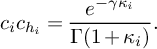 $$ \begin{align} c_ic_{h_i} = \frac{e^{-\gamma \kappa_i}}{\Gamma(1+\kappa_i)}. \end{align} $$
Therefore, the ratio of the constants in the bounds for $S_1$
and
$S_1$
and $S_4^{(i)}$
is
$S_4^{(i)}$
is $\kappa _ic_icc_{h_i}AA_i/cB$
, which is independent of S and tends to zero as
$\kappa _ic_icc_{h_i}AA_i/cB$
, which is independent of S and tends to zero as $\alpha \rightarrow 0$
. Also,
$\alpha \rightarrow 0$
. Also,
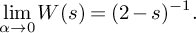 $$ \begin{align*}\lim_{\alpha \rightarrow 0}W(s) = (2-s)^{-1}.\end{align*} $$
Therefore,
 $$ \begin{align} \lim_{\alpha \rightarrow 0}S_4^{(i)} \ll \frac{(B+o(1))X}{(\log N)^{\kappa}}\left(\log 2-\log \beta_i\right). \end{align} $$
For all $\epsilon>0$
, by choosing
$\epsilon>0$
, by choosing $\beta _i$
sufficiently close to
$\beta _i$
sufficiently close to $2$
, we have the bound
$2$
, we have the bound
 $$ \begin{align} \lim_{\alpha \rightarrow 0}S_4^{(i)} \leqslant \frac{(\epsilon B+o(1)) X}{(\log N)^{\kappa}}\ll \epsilon S_1. \end{align} $$
We recall from Sections 4.4 and 4.5 that $S_2^{(i)}$
and
$S_2^{(i)}$
and $S_3^{(i)}$
are also negligible compared to
$S_3^{(i)}$
are also negligible compared to $S_1$
as
$S_1$
as $\alpha \rightarrow 0$
. Therefore, we see that
$\alpha \rightarrow 0$
. Therefore, we see that $S(\mathcal {A},\mathcal {P},x)>0$
for sufficiently small
$S(\mathcal {A},\mathcal {P},x)>0$
for sufficiently small $\alpha $
and sufficiently large N.
$\alpha $
and sufficiently large N.
To obtain the best quantitative bounds, the choices of $\beta _i \in (1,2)$
should be optimised so as to minimise
$\beta _i \in (1,2)$
should be optimised so as to minimise $S_3^{(i)}+S_4^{(i)}$
. However, in practice, numerical computations suggest that the optimal choices for
$S_3^{(i)}+S_4^{(i)}$
. However, in practice, numerical computations suggest that the optimal choices for $\beta _i$
are extremely close to
$\beta _i$
are extremely close to $2$
, and little is lost in taking them arbitrarily close to 2, as above. In this case, the contributions from the sums
$2$
, and little is lost in taking them arbitrarily close to 2, as above. In this case, the contributions from the sums $S_4^{(i)}$
are negligible. Taking a sum over i of the estimates from (4.37) and combining with (4.25), for any
$S_4^{(i)}$
are negligible. Taking a sum over i of the estimates from (4.37) and combining with (4.25), for any $\epsilon>0$
, we have
$\epsilon>0$
, we have
 $$ \begin{align*}S(\mathcal{A},\mathcal{P},x) \geqslant \left(\frac{(c-\epsilon+o(1))X}{(\log N)^{\kappa}}\right)\left(B-A\alpha \sum_{i=m+1}^k \theta_i \int_{1}^{2}(2-s)^{-\kappa}\frac{\textrm{d}s}{s}\right).\end{align*} $$
Let $r(\kappa ) = B/A$
. Then we have established that
$r(\kappa ) = B/A$
. Then we have established that $S(\mathcal {A}, \mathcal {P}, x)>0$
provided that
$S(\mathcal {A}, \mathcal {P}, x)>0$
provided that
 $$ \begin{align} r(\kappa) - \alpha\sum_{i=m+1}^k \theta_i\int_{1}^{2}(2-s)^{-\kappa}\frac{\textrm{d}s}{s}>0. \end{align} $$
We recall that $\theta = \theta _0 + \cdots +\theta _k$
and
$\theta = \theta _0 + \cdots +\theta _k$
and $\kappa = \alpha \theta $
. Therefore, we may replace
$\kappa = \alpha \theta $
. Therefore, we may replace $\alpha \sum _{i=m+1}^k\theta _i$
with the trivial upper bound
$\alpha \sum _{i=m+1}^k\theta _i$
with the trivial upper bound $\kappa $
, after which we find by numerical computations (see Section 4.9 for details) that the largest value of
$\kappa $
, after which we find by numerical computations (see Section 4.9 for details) that the largest value of $\kappa $
we can take in (4.55) is
$\kappa $
we can take in (4.55) is $\kappa = 0.39000\ldots $
. Thus the condition
$\kappa = 0.39000\ldots $
. Thus the condition $\alpha \theta \leqslant 0.39$
is enough to ensure that
$\alpha \theta \leqslant 0.39$
is enough to ensure that $S(\mathcal {A}, \mathcal {P},x)>0$
for sufficiently large N. This completes the proof of Theorem 2.1.
$S(\mathcal {A}, \mathcal {P},x)>0$
for sufficiently large N. This completes the proof of Theorem 2.1.
4.8 Proof of Theorem 2.3
We now discuss the case $d=3$
, where
$d=3$
, where $f(x,y)$
may contain irreducible factors of degree up to
$f(x,y)$
may contain irreducible factors of degree up to $3$
. We recall in the case
$3$
. We recall in the case $d=2$
, the sums
$d=2$
, the sums $S_4^{(i)}$
could be made negligible compared to
$S_4^{(i)}$
could be made negligible compared to $S_1$
by choosing
$S_1$
by choosing $\beta _i$
arbitrarily close to
$\beta _i$
arbitrarily close to $2$
, due to the factor
$2$
, due to the factor $\log 2- \log \beta _i$
appearing in (4.53). When
$\log 2- \log \beta _i$
appearing in (4.53). When $d=3$
, we obtain the same bound as in (4.53), but with
$d=3$
, we obtain the same bound as in (4.53), but with $\log 2-\log \beta _i$
replaced with
$\log 2-\log \beta _i$
replaced with $\log 2 - \log (\beta _i-1)$
. Consequently,
$\log 2 - \log (\beta _i-1)$
. Consequently, $S_4^{(i)}$
is no longer negligible, even when
$S_4^{(i)}$
is no longer negligible, even when $\alpha \rightarrow 0$
and
$\alpha \rightarrow 0$
and $\beta _i$
is arbitrarily close to
$\beta _i$
is arbitrarily close to $2$
. In fact, it can be checked that its limit as
$2$
. In fact, it can be checked that its limit as $\alpha \rightarrow 0$
and
$\alpha \rightarrow 0$
and $\beta _i \rightarrow 2$
is larger than
$\beta _i \rightarrow 2$
is larger than $S_1$
, and so the above methods break down in this case.
$S_1$
, and so the above methods break down in this case.
However, we recall the additional hypothesis in Theorem 2.3 that Assumption 2.2 holds. By enlarging $\mathcal {P}$
if necessary, we may assume that equality holds in (2.9) – namely,
$\mathcal {P}$
if necessary, we may assume that equality holds in (2.9) – namely,
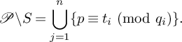 $$\begin{align*}\mathcal{P}\backslash S = \bigcup_{j=1}^n \{p \equiv t_i \ (\mathrm{mod}\ q_i)\}. \end{align*}$$
By Dirichlet’s theorem on primes in arithmetic progressions, (2.4) holds with $\alpha \leqslant \sum _{j=1}^n \frac {1}{q_j-1} \leqslant 0.32380$
. Moreover, it follows from Lemma 5.8 (a version of the Chebotarev density theorem) that (2.5) holds for some
$\alpha \leqslant \sum _{j=1}^n \frac {1}{q_j-1} \leqslant 0.32380$
. Moreover, it follows from Lemma 5.8 (a version of the Chebotarev density theorem) that (2.5) holds for some $\theta _i \leqslant 3$
. We now explain why this choice of
$\theta _i \leqslant 3$
. We now explain why this choice of $\mathcal {P}$
is easier to handle than arbitrary choices of
$\mathcal {P}$
is easier to handle than arbitrary choices of $\mathcal {P}$
of the same density
$\mathcal {P}$
of the same density $\alpha $
.
$\alpha $
.
When applying the switching principle for $S_4^{(i)}$
, we wrote
$S_4^{(i)}$
, we wrote $f_i(a,b) = pr$
for
$f_i(a,b) = pr$
for $p \in \mathcal {P}$
. Since we may assume
$p \in \mathcal {P}$
. Since we may assume $q_1, \ldots , q_n \in S_0$
, the congruence condition
$q_1, \ldots , q_n \in S_0$
, the congruence condition $C(a,b)$
forces
$C(a,b)$
forces $f_i(a,b)$
to lie in a particular congruence class modulo
$f_i(a,b)$
to lie in a particular congruence class modulo $q_1, \ldots , q_n$
. Combined with the fact that
$q_1, \ldots , q_n$
. Combined with the fact that $p \equiv t_j \ (\mathrm {mod}\ q_j)$
for some j, we see that r lies in a particular congruence class modulo
$p \equiv t_j \ (\mathrm {mod}\ q_j)$
for some j, we see that r lies in a particular congruence class modulo $q_j$
for some
$q_j$
for some $j\in \{1, \ldots , n\}$
, and this congruence class depends only on
$j\in \{1, \ldots , n\}$
, and this congruence class depends only on $t_j, C(a,b)$
and f. Moreover, by (4.26), we have that
$t_j, C(a,b)$
and f. Moreover, by (4.26), we have that $\gcd (r, \Delta ) = \gcd (f_i(a_0,b_0),\Delta )$
depends only on
$\gcd (r, \Delta ) = \gcd (f_i(a_0,b_0),\Delta )$
depends only on $C(a,b)$
and f. We deduce that there exist
$C(a,b)$
and f. We deduce that there exist $r_1,\ldots , r_n$
, depending only on
$r_1,\ldots , r_n$
, depending only on $t_1, \ldots , t_n, C(a,b)$
and f, such that
$t_1, \ldots , t_n, C(a,b)$
and f, such that $r':= |r|/\gcd (r,\Delta )$
lies in the set
$r':= |r|/\gcd (r,\Delta )$
lies in the set
 $$\begin{align*}\mathcal{T} := \{r' \in \mathbb{N}: r'\equiv r_j \ (\mathrm{mod}\ q_j) \textrm{ for some }j\in\{1, \ldots, n\}\}. \end{align*}$$
Adding this condition into (4.43) and (4.44) and changing notation from $r'$
back to r, we obtain
$r'$
back to r, we obtain
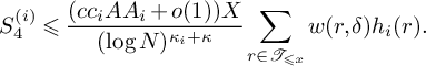 $$ \begin{align} S_4^{(i)}\leqslant \frac{(cc_iAA_i+o(1))X}{(\log N)^{\kappa_i+\kappa}}\sum_{r \in \mathcal{T}_{\leqslant x}}w(r,\delta)h_i(r). \end{align} $$
As demonstrated by Irving [Reference Irving27, Lemma 6.1], the argument based on [Reference Friedlander and Iwaniec18, Theorem A.5] we used to obtain (4.46) can be generalised to give
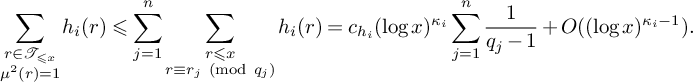 $$ \begin{align} \sum_{\substack{r \in \mathcal{T}_{\leqslant x}\\ \mu^2(r)=1}}h_i(r) \leqslant \sum_{j=1}^n \sum_{\substack{r \leqslant x\\ r\equiv r_j \ (\mathrm{mod}\ q_j)}}h_i(r) = c_{h_i}(\log x)^{\kappa_i}\sum_{j=1}^n \frac{1}{q_j-1} + O((\log x)^{\kappa_i-1}). \end{align} $$
Proceeding as before, we deduce the same estimate for $S_4^{(i)}$
as in (4.50), but with an additional factor
$S_4^{(i)}$
as in (4.50), but with an additional factor $\alpha _0 := \sum _{j=1}^n \frac {1}{q_j-1}$
. It is now clear qualitatively that for sufficiently large
$\alpha _0 := \sum _{j=1}^n \frac {1}{q_j-1}$
. It is now clear qualitatively that for sufficiently large $q_1, \ldots , q_n$
(i.e., as
$q_1, \ldots , q_n$
(i.e., as $\alpha _0 \rightarrow 0$
), the sums
$\alpha _0 \rightarrow 0$
), the sums $S_4^{(i)}$
are once again negligible compared to
$S_4^{(i)}$
are once again negligible compared to $S_1$
.
$S_1$
.
We now make the above discussion more quantitative in order to complete the proof of Theorem 2.3. Combining everything, we see that $S(\mathcal {A},\mathcal {P},x)>0$
for sufficiently large N provided that
$S(\mathcal {A},\mathcal {P},x)>0$
for sufficiently large N provided that
 $$ \begin{align}r(\kappa)-\sum_{i\,:\, \deg f_i =2}\alpha \theta_i \int_{1}^2(2-s)^{-\kappa}\frac{\textrm{d}s}{s}- \sum_{\substack{i \,:\, \deg f_i =3}}\alpha_0 A_i\kappa_ic_ic_{h_i}\int_{0}^1 W(s) \textrm{d}s>0. \end{align} $$
We denote the left-hand side of (4.58) by $F(\boldsymbol {\theta })$
. Recalling (4.51) and (4.52), we have
$F(\boldsymbol {\theta })$
. Recalling (4.51) and (4.52), we have
 $$ \begin{align} A_i\kappa_ic_ic_{h_i}\int_{0}^1 W(s) \textrm{d}s = \frac{A_i\kappa_ie^{-\gamma \kappa_i}\kappa^{-\kappa}\kappa_i^{-\kappa_i}(\kappa+\kappa_i)^{\kappa+\kappa_i}}{\Gamma(1+\kappa_i)}\int_0^1 (2-s)^{-(\kappa+\kappa_i)}s^{\kappa_i-1}\textrm{d}s. \end{align} $$
For a fixed choice of $\kappa <1/2$
, the integrand is a decreasing function of
$\kappa <1/2$
, the integrand is a decreasing function of $\kappa _i$
because
$\kappa _i$
because $0\leqslant \frac {s}{(2-s)}\leqslant 1$
for any
$0\leqslant \frac {s}{(2-s)}\leqslant 1$
for any $s\in [0,1]$
. The functions
$s\in [0,1]$
. The functions $\Gamma (1+\kappa _i)^{-1}$
,
$\Gamma (1+\kappa _i)^{-1}$
, $\kappa _i^{-\kappa _i}$
and
$\kappa _i^{-\kappa _i}$
and $e^{-\gamma \kappa _i}$
are also decreasing in
$e^{-\gamma \kappa _i}$
are also decreasing in $\kappa _i$
in the range
$\kappa _i$
in the range $\kappa _i\in (1/2,1)$
. Let
$\kappa _i\in (1/2,1)$
. Let $t = \alpha _0 \deg f$
. Since
$t = \alpha _0 \deg f$
. Since $\kappa _i \geqslant 1-\kappa \geqslant 1-t$
, we therefore obtain an upper bound by replacing
$\kappa _i \geqslant 1-\kappa \geqslant 1-t$
, we therefore obtain an upper bound by replacing $\kappa _i$
with
$\kappa _i$
with $1-t$
in all these terms. The remaining terms in (4.59) are all increasing in
$1-t$
in all these terms. The remaining terms in (4.59) are all increasing in $\kappa _i$
, and we apply the trivial bound
$\kappa _i$
, and we apply the trivial bound $\kappa _i \leqslant 1$
. Finally, we note that
$\kappa _i \leqslant 1$
. Finally, we note that $\kappa ^{-\kappa }(\kappa +\kappa _i)^{\kappa +\kappa _i}$
is an increasing function in
$\kappa ^{-\kappa }(\kappa +\kappa _i)^{\kappa +\kappa _i}$
is an increasing function in $\kappa $
for
$\kappa $
for $\kappa <1/2$
, and so we may replace
$\kappa <1/2$
, and so we may replace $\kappa $
by t in this expression. Therefore, (4.59) can be bounded by
$\kappa $
by t in this expression. Therefore, (4.59) can be bounded by
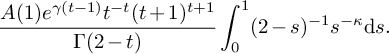 $$ \begin{align} \frac{A(1)e^{\gamma(t-1)}t^{-t}(t+1)^{t+1}}{\Gamma(2-t)}\int_{0}^1 (2-s)^{-1}s^{-\kappa}\textrm{d}s. \end{align} $$
We denote the factor outside the integral in (4.60) by $H(t)$
. The integral in (4.60) is equal to the first integral in (4.58), as can be seen by making the substitution
$H(t)$
. The integral in (4.60) is equal to the first integral in (4.58), as can be seen by making the substitution $u=2-s$
. Therefore,
$u=2-s$
. Therefore,
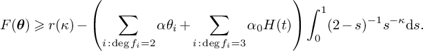 $$ \begin{align*} F(\boldsymbol{\theta})&\geqslant r(\kappa)-\left(\sum_{i\,:\,\deg f_i =2}\alpha\theta_i + \sum_{i\,:\, \deg f_i = 3} \alpha_0 H(t)\right) \int_0^1 (2-s)^{-1}s^{-\kappa}\textrm{d}s. \end{align*} $$
Recalling that $A(1)=2e^{\gamma }$
, it can be checked that
$A(1)=2e^{\gamma }$
, it can be checked that $H(t)>4$
for all
$H(t)>4$
for all $t>0.2$
, and so in particular,
$t>0.2$
, and so in particular, $H(t)>2\theta _i$
whenever
$H(t)>2\theta _i$
whenever $\deg f_i =2$
. Moreover, r is a decreasing function of
$\deg f_i =2$
. Moreover, r is a decreasing function of $\kappa $
, so
$\kappa $
, so $r(\kappa )\geqslant r(t)$
. We obtain
$r(\kappa )\geqslant r(t)$
. We obtain
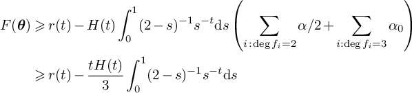 $$ \begin{align} F(\boldsymbol{\theta})&\geqslant r(t)-H(t)\int_{0}^1 (2-s)^{-1}s^{-t}\textrm{d}s\left(\sum_{i\,:\,\deg f_i=2}\alpha/2 +\sum_{\substack{i:\deg f_i =3}}\alpha_0\right)\nonumber\\ &\geqslant r(t)-\frac{tH(t)}{3}\int_{0}^1 (2-s)^{-1}s^{-t}\textrm{d}s \end{align} $$
for any $t>0.2$
. We find by numerical computations that the above expression is positive provided that
$t>0.2$
. We find by numerical computations that the above expression is positive provided that $t\leqslant 0.32380.$
. Since
$t\leqslant 0.32380.$
. Since $t= \alpha _0\deg f$
, this is implied by the condition (2.9) assumed in Theorem 2.3.
$t= \alpha _0\deg f$
, this is implied by the condition (2.9) assumed in Theorem 2.3.
4.9 Details of the numerical computations
We now explain how we obtained numerical values with guaranteed error bounds in the proofs of Theorem 2.1 and Theorem 2.3. From [Reference Friedlander and Iwaniec18, Equations (11.62), (11.63)], we have for $0< \kappa < 1/2$
that
$0< \kappa < 1/2$
that
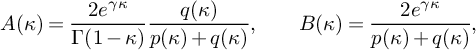 $$\begin{align*}A(\kappa) = \frac{2e^{\gamma\kappa}}{\Gamma(1-\kappa)}\frac{q(\kappa)}{p(\kappa)+ q(\kappa)}, \qquad B(\kappa) = \frac{2e^{\gamma \kappa}}{p(\kappa) + q(\kappa)}, \end{align*}$$
where
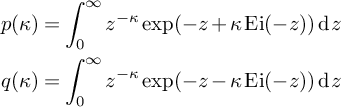 $$ \begin{align*} p(\kappa) &= \int_{0}^{\infty}z^{-\kappa}\exp(-z+\kappa\operatorname{Ei}(-z))\operatorname{d}z \\ q(\kappa) &=\int_{0}^{\infty}z^{-\kappa}\exp(-z-\kappa\operatorname{Ei}(-z))\operatorname{d}z \end{align*} $$
and where $\operatorname {Ei}(-z) = -\int _{z}^{\infty }\frac {e^{-u}}{u}\operatorname {d}u$
is the standard exponential integral. For any
$\operatorname {Ei}(-z) = -\int _{z}^{\infty }\frac {e^{-u}}{u}\operatorname {d}u$
is the standard exponential integral. For any $0<\kappa < 1/2$
, the integrand defining
$0<\kappa < 1/2$
, the integrand defining $p(\kappa )$
is monotonically decreasing, decays exponentially as
$p(\kappa )$
is monotonically decreasing, decays exponentially as $z \rightarrow \infty $
, and is bounded above by
$z \rightarrow \infty $
, and is bounded above by $2$
. Similarly, the integrand defining
$2$
. Similarly, the integrand defining $q(\kappa )$
is monotonically decreasing and decays exponentially as
$q(\kappa )$
is monotonically decreasing and decays exponentially as $z \rightarrow \infty $
, but diverges as
$z \rightarrow \infty $
, but diverges as $z \rightarrow 0$
. To analyse its behaviour near
$z \rightarrow 0$
. To analyse its behaviour near $0$
, we note that for
$0$
, we note that for $\delta \in (0,1)$
and
$\delta \in (0,1)$
and $\kappa < 0.4$
, we have
$\kappa < 0.4$
, we have
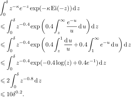 $$ \begin{align*} &\int_{0}^{\delta}z^{-\kappa}e^{-z}\exp(-\kappa\operatorname{Ei}(-z))\operatorname{d}z\\ &\leqslant \int_{0}^{\delta}z^{-0.4}\operatorname{exp}\left(0.4\int_{z}^{\infty}\frac{e^{-u}}{u}\operatorname{d}u\right)\operatorname{d}z\\ &\leqslant \int_{0}^{\delta}z^{-0.4} \operatorname{exp}\left(0.4\int_{z}^{1}\frac{\operatorname{d}u}{u} + 0.4\int_{1}^{\infty}e^{-u}\operatorname{d}u\right)\operatorname{d}z\\ &\leqslant \int_{0}^{\delta}z^{-0.4}\exp(-0.4\log(z) + 0.4e^{-1})\operatorname{d}z\\ &\leqslant 2 \int_{0}^{\delta}z^{-0.8}\operatorname{d}z\\ &\leqslant 10\delta^{0.2}. \end{align*} $$
Therefore, we can obtain estimates for $p(\kappa ), q(\kappa )$
(and hence also
$p(\kappa ), q(\kappa )$
(and hence also $A(\kappa ), B(\kappa )$
with provable error bounds using standard numerical integration methods such as the trapezoid rule. The functions from (4.55) and (4.61) are bounded, continuous, and monotonically decreasing in
$A(\kappa ), B(\kappa )$
with provable error bounds using standard numerical integration methods such as the trapezoid rule. The functions from (4.55) and (4.61) are bounded, continuous, and monotonically decreasing in $\kappa $
, and so it is straightforward to find their roots to the desired precision. This was implemented in Sage, which produced the values
$\kappa $
, and so it is straightforward to find their roots to the desired precision. This was implemented in Sage, which produced the values $0.39000, 0.32380$
correct to five decimal places in
$0.39000, 0.32380$
correct to five decimal places in $12.3$
seconds on a standard laptop with
$12.3$
seconds on a standard laptop with $2$
cores.
$2$
cores.
5 Application to the Hasse principle
In this section, we apply the main sieve results (Theorem 2.1 and Theorem 2.3) obtained in Section 4 in order to prove Theorem 1.1 and Theorem 1.3.
5.1 Algebraic reduction of the problem
Let K be a number field of degree n satisfying the Hasse norm principle. In [Reference Irving27, Lemma 2.6], Irving turns the problem of establishing the Hasse principle for
 $$ \begin{align} f(t) = \mathbf{N}(x_1, \ldots, x_n) \neq 0 \end{align} $$
into a sieve problem. Irving assumes that $f(t) \in \mathbb {Z}[t]$
is an irreducible cubic polynomial. However, in the following result, we demonstrate that Irving’s strategy can be applied to establish a similar result for an arbitrary polynomial
$f(t) \in \mathbb {Z}[t]$
is an irreducible cubic polynomial. However, in the following result, we demonstrate that Irving’s strategy can be applied to establish a similar result for an arbitrary polynomial $f\in \mathbb {Z}[t]$
. We recall that
$f\in \mathbb {Z}[t]$
. We recall that $f(x,y)$
denotes the homogenisation of f. Throughout this section, we make the choice
$f(x,y)$
denotes the homogenisation of f. Throughout this section, we make the choice
 $$ \begin{align} \mathcal{P} = \{p \notin S: \textrm{ the inertia degrees of }p\textrm{ in }K/\mathbb{Q}\textrm{ are not coprime}\} \end{align} $$
for a finite set of primes S containing all ramified primes in $K/\mathbb {Q}$
.
$K/\mathbb {Q}$
.
Proposition 5.1. Suppose that (5.1) has solutions over $\mathbb {Q}_p$
for every p and over
$\mathbb {Q}_p$
for every p and over $\mathbb {R}$
. Let
$\mathbb {R}$
. Let $\mathcal {P}$
and S be as in (5.2). Then there exists
$\mathcal {P}$
and S be as in (5.2). Then there exists $\Delta \in \mathbb {N}$
, divisible only by primes in S, integers
$\Delta \in \mathbb {N}$
, divisible only by primes in S, integers $a_0,b_0$
, and real numbers
$a_0,b_0$
, and real numbers $r,\xi>0$
such that the following implication holds:
$r,\xi>0$
such that the following implication holds:
Suppose that $a,b$
are integers for which
$a,b$
are integers for which
-
(1)
$a \equiv a_0 \ (\mathrm {mod}\ \Delta )$
and
$b \equiv b_0 \ (\mathrm {mod}\ \Delta )$
, -
(2)
$|a/b - r|<\xi $
, -
(3)
$bf(a,b)$
has no prime factors in
$\mathcal {P}$
.


Then (5.1) has a solution over $\mathbb {Q}$
.
$\mathbb {Q}$
.
By multiplicativity of norms, it suffices to find integers $a,b$
such that b and
$a,b$
such that b and $f(a,b)$
are in
$f(a,b)$
are in $N_{K/\mathbb {Q}}(K^*)$
. Since K satisfies the Hasse norm principle, we have
$N_{K/\mathbb {Q}}(K^*)$
. Since K satisfies the Hasse norm principle, we have $\mathbb {Q}^*\cap N_{K/\mathbb {Q}}(I_K) = N_{K/\mathbb {Q}}(K^*)$
, where
$\mathbb {Q}^*\cap N_{K/\mathbb {Q}}(I_K) = N_{K/\mathbb {Q}}(K^*)$
, where $I_K$
denotes the ideles of K. Consequently, to show that
$I_K$
denotes the ideles of K. Consequently, to show that $c\in \mathbb {Q}^*$
is a norm from K, it suffices to find elements
$c\in \mathbb {Q}^*$
is a norm from K, it suffices to find elements $x_v \in K_v^{*}$
for each place v of K, such that
$x_v \in K_v^{*}$
for each place v of K, such that
-
(1) For all but finitely many places v of K, we have
$x_v\in \mathcal {O}_v^*$
(this ensures that
$(x_v) \in I_K$
). -
(2) For all places w of
$\mathbb {Q}$
, we have (5.3)
$$ \begin{align} \prod_{v\mid w}N_{K_v/\mathbb{Q}_w}(x_v)=c. \end{align} $$


The arguments in [Reference Irving27, Lemma 2.2, Lemma 2.3, Lemma 2.4] go through without changes. We summarise them below.
Lemma 5.2. Suppose $c\neq 0$
is an integer. Then
$c\neq 0$
is an integer. Then
-
(1) If
$p\nmid c$
and
$K/\mathbb {Q}$
is unramified at p, then there exist
$x_v \in \mathcal {O}_v^*$
for each place v of K above p, such that
$\prod _{v\mid p}N_{K_v/\mathbb {Q}_p}(x_v)=c$
. -
(2) Suppose that
$K/\mathbb {Q}$
is unramified at p, and that the inertia degrees above p in K are coprime. Then there exist
$x_v \in K_v^*$
for each place v of K above p, such that
$\prod _{v\mid p}N_{K_v/\mathbb {Q}_p}(x_v)=c$
. -
(3) Let p be a place of
$\mathbb {Q}$
. Suppose that there exists
$x_1, \ldots , x_n \in \mathbb {Q}_p$
such that
$c =\mathbf {N}(x_1, \ldots ,x_n)$
. Then there exists
$x_v \in K_v^*$
for each place v of K above p, such that
$\prod _{v\mid p}N_{K_v/\mathbb {Q}_p}(x_v)=c$
.


We now give a slight generalisation of [Reference Irving27, Lemma 2.5] to the case of an arbitrary polynomial f.
Lemma 5.3. Let p be a prime for which $f(t) = \mathbf {N}(x_1, \ldots , x_n) \neq 0$
has a solution over
$f(t) = \mathbf {N}(x_1, \ldots , x_n) \neq 0$
has a solution over $\mathbb {Q}_p$
. Then there exists
$\mathbb {Q}_p$
. Then there exists $a_0,b_0 \in \mathbb {Z}$
and
$a_0,b_0 \in \mathbb {Z}$
and $l \in \mathbb {N}$
(all depending on p) such that for any
$l \in \mathbb {N}$
(all depending on p) such that for any $a,b \in \mathbb {Z}$
satisfying
$a,b \in \mathbb {Z}$
satisfying $a\equiv a_0 \ (\mathrm {mod}\ p^l), b\equiv b_0 \ (\mathrm {mod}\ p^l)$
, we have
$a\equiv a_0 \ (\mathrm {mod}\ p^l), b\equiv b_0 \ (\mathrm {mod}\ p^l)$
, we have $b,f(a,b) \in \mathbf {N}(\mathbb {Q}_p^n)\backslash \{0\}$
.
$b,f(a,b) \in \mathbf {N}(\mathbb {Q}_p^n)\backslash \{0\}$
.
Proof. We define $N = \mathbf {N}(\mathbb {Q}_p^n)\backslash \{0\}$
. Let
$N = \mathbf {N}(\mathbb {Q}_p^n)\backslash \{0\}$
. Let $t_1 \in \mathbb {Q}_p$
be such that
$t_1 \in \mathbb {Q}_p$
be such that $f(t_1) = \mathbf {N}(x_1, \ldots , x_n) \neq 0$
has a solution over
$f(t_1) = \mathbf {N}(x_1, \ldots , x_n) \neq 0$
has a solution over $\mathbb {Q}_p$
. Choose
$\mathbb {Q}_p$
. Choose $a_1, b_1 \in \mathbb {Z}_p$
such that
$a_1, b_1 \in \mathbb {Z}_p$
such that $\nu _p(b_1)$
is a multiple of n, and
$\nu _p(b_1)$
is a multiple of n, and $a_1/b_1 = t_1$
. Then
$a_1/b_1 = t_1$
. Then $b_1 \in N$
and
$b_1 \in N$
and $f(a_1,b_1) \in N$
.
$f(a_1,b_1) \in N$
.
The set $N \subseteq \mathbb {Q}_p$
is open, and so
$N \subseteq \mathbb {Q}_p$
is open, and so $N\times N \subseteq \mathbb {Q}_p^2$
is open. Moreover, the map
$N\times N \subseteq \mathbb {Q}_p^2$
is open. Moreover, the map $\varphi : \mathbb {Q}_p^2 \rightarrow \mathbb {Q}_p^2$
sending
$\varphi : \mathbb {Q}_p^2 \rightarrow \mathbb {Q}_p^2$
sending $(a,b)$
to
$(a,b)$
to $(f(a,b),b)$
is continuous in the p-adic topology. Therefore, the set
$(f(a,b),b)$
is continuous in the p-adic topology. Therefore, the set $\varphi ^{-1}(N\times N)$
is open, and contains the element
$\varphi ^{-1}(N\times N)$
is open, and contains the element $(a_1,b_1)$
. Hence, there is a small p-adic ball with centre
$(a_1,b_1)$
. Hence, there is a small p-adic ball with centre $(a_1,b_1)$
, all of whose elements
$(a_1,b_1)$
, all of whose elements $(a,b)$
satisfy
$(a,b)$
satisfy $b, f(a,b) \in N$
. This ball can be described by congruence conditions
$b, f(a,b) \in N$
. This ball can be described by congruence conditions $a\equiv a_0 \ (\mathrm {mod}\ p^l), b\equiv b_0 \ (\mathrm {mod}\ p^l)$
for a sufficiently large integer l, as claimed in the lemma.
$a\equiv a_0 \ (\mathrm {mod}\ p^l), b\equiv b_0 \ (\mathrm {mod}\ p^l)$
for a sufficiently large integer l, as claimed in the lemma.
Proof of Proposition 5.1
The proof closely follows the argument in [Reference Irving27, Lemma 2.6]. By the Hasse norm principle, to find solutions to (5.1), it suffices to find integers $a,b$
such that properties (1) and (2) stated before Lemma 5.2 hold with
$a,b$
such that properties (1) and (2) stated before Lemma 5.2 hold with $c=b$
and
$c=b$
and $c=f(a,b)$
. We divide the places of
$c=f(a,b)$
. We divide the places of $\mathbb {Q}$
into four sets:
$\mathbb {Q}$
into four sets:
-
(1)
$p\in S$
. Here, Lemma 5.3 gives congruence conditions
$a \equiv a_{0,p} \ (\mathrm {mod}\ p^l)$
,
$b \equiv b_{0,p} \ (\mathrm {mod}\ p^l)$
which ensure that
$b, f(a,b) \in N(\mathbb {Q}_p^n)\backslash \{0\}$
. By part (3) of Lemma 5.2, we deduce that property (2) stated before Lemma 5.2 holds with
$c=b$
and
$c=f(a,b)$
. The congruence conditions at each prime
$p \in S$
can be merged into one congruence condition
$a \equiv a_0 \ (\mathrm {mod}\ \Delta ), b \equiv b_0 \ (\mathrm {mod}\ \Delta )$
using the Chinese remainder theorem. -
(2)
$p\notin S$
and
$p\notin \mathcal {P}$
. If
$p \nmid b$
, we apply part (1) of Lemma 5.2 with
$c=b$
. If
$p\mid b$
, we apply part (2) of Lemma 5.2 with
$c=b$
. The same argument works for
$f(a,b)$
by choosing
$c=f(a,b)$
. -
(3)
$p \in \mathcal {P}$
. Since we are assuming that
$bf(a,b)$
has no prime factors in
$\mathcal {P}$
, for these primes, part (1) of Lemma 5.2 applies with
$c=b$
and
$c=f(a,b)$
. -
(4)
$p=\infty $
. We follow a similar argument to Lemma 5.3. We may assume that (5.1) is everywhere locally soluble, so in particular, there exists
$r \in \mathbb {R}$
such that
$f(r) \in \mathbf {N}(\mathbb {R}^n)\backslash \{0\}$
. Since f is continuous and
$\mathbf {N}(\mathbb {R}^n)\backslash \{0\}$
is open in the Euclidean topology, we can find
$\xi>0$
such that
$f(t) \in \mathbf {N}(\mathbb {R}^n)\backslash \{0\}$
whenever
$|t-r|<\xi $
. Clearly, solubility of
$f(t) = \mathbf {N}(\mathbf {x}) \neq 0$
and
$f(-t) = \mathbf {N}(\mathbf {x}) \neq 0$
over
$\mathbb {Q}$
are equivalent; consequently, we may assume
$r>0$
. Suppose in addition that
$t\in \mathbb {Q}$
, and write
$t=a/b$
for
$a,b \in \mathbb {N}$
. Since b is positive, it is automatically in
$\mathbf {N}(\mathbb {R}^n)\backslash \{0\}$
. By multiplicativity of norms, we conclude that
$b,f(a,b) \in \mathbf {N}(\mathbb {R}^n)\backslash \{0\}$
. The condition (5.3) now follows from part (3) of Lemma 5.2.


Example 5.4. Let $f(t) = (t^2-2)(-t^2+3)$
and
$f(t) = (t^2-2)(-t^2+3)$
and $K = \mathbb {Q}(i)$
, so that
$K = \mathbb {Q}(i)$
, so that
 $$ \begin{align*} f(x,y) &= (x^2-2y^2)(-x^2+3y^2)\\ N_{K/\mathbb{Q}}(u,v) &= u^2+v^2. \end{align*} $$
It is known that there is a Brauer–Manin obstruction to the Hasse principle for the equation $(t^2-2)(-t^2+3) = u^2+v^2 \neq 0$
by the work of Iskovskikh [Reference Iskovskikh28]. However, Proposition 5.1 still applies.
$(t^2-2)(-t^2+3) = u^2+v^2 \neq 0$
by the work of Iskovskikh [Reference Iskovskikh28]. However, Proposition 5.1 still applies.
When $p\equiv 1 \ (\mathrm {mod}\ 4)$
, the prime p splits in
$p\equiv 1 \ (\mathrm {mod}\ 4)$
, the prime p splits in $K/\mathbb {Q}$
, and so the inertia degrees of p in
$K/\mathbb {Q}$
, and so the inertia degrees of p in $K/\mathbb {Q}$
are coprime. However, when
$K/\mathbb {Q}$
are coprime. However, when $p \equiv 3 \ (\mathrm {mod}\ 4)$
, the prime p is inert in
$p \equiv 3 \ (\mathrm {mod}\ 4)$
, the prime p is inert in $K/\mathbb {Q}$
and has degree 2, so the inertia degrees are not coprime. Therefore, we have
$K/\mathbb {Q}$
and has degree 2, so the inertia degrees are not coprime. Therefore, we have $\mathcal {P} = \{p: p\equiv 3 \ (\mathrm {mod}\ 4)\}$
. We choose
$\mathcal {P} = \{p: p\equiv 3 \ (\mathrm {mod}\ 4)\}$
. We choose $S=\{2\}$
. In this example, it can be checked that the congruence conditions
$S=\{2\}$
. In this example, it can be checked that the congruence conditions $a \equiv 8 \ (\mathrm {mod}\ 16)$
and
$a \equiv 8 \ (\mathrm {mod}\ 16)$
and $b \equiv 1 \ (\mathrm {mod}\ 16)$
are sufficient. Finally, for the infinite place, we just have the condition
$b \equiv 1 \ (\mathrm {mod}\ 16)$
are sufficient. Finally, for the infinite place, we just have the condition $f(a,b)>0$
. The sieve problem we obtain is to find integers
$f(a,b)>0$
. The sieve problem we obtain is to find integers $a,b$
such that
$a,b$
such that
-
(1)
$a \equiv 8 \ (\mathrm {mod}\ 16), b \equiv 1 \ (\mathrm {mod}\ 16)$
, -
(2)
$f(a,b)>0$
, -
(3)
$f(a,b)$
has no prime factors
$p \equiv 3 \ (\mathrm {mod}\ 4)$
.


We remark that $f(a/b) = b^{-4}f(a,b)$
, and since
$f(a/b) = b^{-4}f(a,b)$
, and since $2=[K:\mathbb {Q}]$
divides
$2=[K:\mathbb {Q}]$
divides $4$
,
$4$
, $b^{-4}$
is automatically a norm from K. This explains why in (3) above, we can consider prime factors of
$b^{-4}$
is automatically a norm from K. This explains why in (3) above, we can consider prime factors of $f(a,b)$
rather than
$f(a,b)$
rather than $bf(a,b)$
.
$bf(a,b)$
.
An integer is the sum of two squares if and only if it is non-negative and all prime factors $p \equiv 3 \ (\mathrm {mod}\ 4)$
occur with an even exponent. The above conditions are stronger than this, so the algebraic reduction performed in Proposition 5.1 is consistent with what we already knew for this example.
$p \equiv 3 \ (\mathrm {mod}\ 4)$
occur with an even exponent. The above conditions are stronger than this, so the algebraic reduction performed in Proposition 5.1 is consistent with what we already knew for this example.
Since the Hasse principle fails for this example, we know that the above sieve problem cannot have a solution. This is indeed the case since condition (1) implies that $-a^2+3b^2 \equiv 3 \ (\mathrm {mod}\ 4)$
, and so
$-a^2+3b^2 \equiv 3 \ (\mathrm {mod}\ 4)$
, and so $f(a,b)$
must contain a prime factor
$f(a,b)$
must contain a prime factor $p \equiv 3 \ (\mathrm {mod}\ 4)$
.
$p \equiv 3 \ (\mathrm {mod}\ 4)$
.
The fact that the above sieve problem has no solutions also does not contradict Theorem 2.1. For a prime $p>3$
, we have that
$p>3$
, we have that $\nu _1(p)$
is 2 if
$\nu _1(p)$
is 2 if $p \equiv \pm 1 \ (\mathrm {mod}\ 8)$
and zero otherwise, and
$p \equiv \pm 1 \ (\mathrm {mod}\ 8)$
and zero otherwise, and $\nu _2(p)$
is 2 if
$\nu _2(p)$
is 2 if $p \equiv \pm 1\ (\mathrm {mod}\ 12)$
and zero otherwise. Consequently, by Dirichlet’s theorem on primes in arithmetic progressions, for
$p \equiv \pm 1\ (\mathrm {mod}\ 12)$
and zero otherwise. Consequently, by Dirichlet’s theorem on primes in arithmetic progressions, for $i\in \{1,2\}$
, asymptotically one half of the primes
$i\in \{1,2\}$
, asymptotically one half of the primes $p\in \mathcal {P}$
have
$p\in \mathcal {P}$
have $\nu _i(p) = 2$
and half have
$\nu _i(p) = 2$
and half have $\nu _i(p) = 0$
. We conclude that
$\nu _i(p) = 0$
. We conclude that $\theta _1 = \theta _2 = 1$
, so that
$\theta _1 = \theta _2 = 1$
, so that $\theta = 2$
. Theorem 2.1 therefore requires the density of
$\theta = 2$
. Theorem 2.1 therefore requires the density of $\mathcal {P}$
to be less than
$\mathcal {P}$
to be less than $0.39000\ldots /\theta =0.19503\ldots $
. However, the density of
$0.39000\ldots /\theta =0.19503\ldots $
. However, the density of $\mathcal {P}$
here is
$\mathcal {P}$
here is $1/2$
, and so Theorem 2.1 does not apply to this example.
$1/2$
, and so Theorem 2.1 does not apply to this example.
5.2 The Chebotarev density theorem
In order to apply the sieve results from Section 2 to prove Theorem 1.1 and Theorem 1.3, we need to compute the densities (2.4) and (2.5) for the choice of $\mathcal {P}$
given in (5.2). For more complicated number fields K, such as when
$\mathcal {P}$
given in (5.2). For more complicated number fields K, such as when $K/\mathbb {Q}$
is non-abelian, it is not possible to write down the set
$K/\mathbb {Q}$
is non-abelian, it is not possible to write down the set $\mathcal {P}$
explicitly in terms of congruence conditions. However, we can still compute the densities (2.4) and (2.5) by appealing to the Chebotarev density theorem, which can be viewed as a vast generalisation of Dirichlet’s theorem on primes in arithmetic progressions.
$\mathcal {P}$
explicitly in terms of congruence conditions. However, we can still compute the densities (2.4) and (2.5) by appealing to the Chebotarev density theorem, which can be viewed as a vast generalisation of Dirichlet’s theorem on primes in arithmetic progressions.
Let $K/\mathbb {Q}$
be a number field of degree n. Let p be a prime, unramified in
$K/\mathbb {Q}$
be a number field of degree n. Let p be a prime, unramified in $K/\mathbb {Q}$
. We can factorise the ideal
$K/\mathbb {Q}$
. We can factorise the ideal $(p)$
as
$(p)$
as $(p) = \mathfrak {p}_1\cdots \mathfrak {p}_r$
, where
$(p) = \mathfrak {p}_1\cdots \mathfrak {p}_r$
, where $\mathfrak {p}_1, \ldots , \mathfrak {p}_r$
are distinct prime ideals in
$\mathfrak {p}_1, \ldots , \mathfrak {p}_r$
are distinct prime ideals in $\mathcal {O}_K$
. The splitting type of p in
$\mathcal {O}_K$
. The splitting type of p in $K/\mathbb {Q}$
is the partition
$K/\mathbb {Q}$
is the partition $(a_1, \ldots ,a_r)$
of n, where
$(a_1, \ldots ,a_r)$
of n, where $a_i$
is the inertia degree of
$a_i$
is the inertia degree of $\mathfrak {p}_i$
(i.e.,
$\mathfrak {p}_i$
(i.e., $N(\mathfrak {p}_i) = p^{a_i}$
). Equivalently, the splitting type is the list of degrees of the irreducible factors of the minimum polynomial of
$N(\mathfrak {p}_i) = p^{a_i}$
). Equivalently, the splitting type is the list of degrees of the irreducible factors of the minimum polynomial of $K/\mathbb {Q}$
, when factorised modulo p.
$K/\mathbb {Q}$
, when factorised modulo p.
Suppose first that $K/\mathbb {Q}$
is Galois, with Galois group G. Then G acts transitively on
$K/\mathbb {Q}$
is Galois, with Galois group G. Then G acts transitively on $\{\mathfrak {p}_1, \ldots , \mathfrak {p}_r\}$
. Fix
$\{\mathfrak {p}_1, \ldots , \mathfrak {p}_r\}$
. Fix $i \in \{1, \ldots , r\}$
. The Decomposition group
$i \in \{1, \ldots , r\}$
. The Decomposition group $D_{\mathfrak {p}_i}$
is the stabilizer of
$D_{\mathfrak {p}_i}$
is the stabilizer of $\mathfrak {p}_i$
under this action. Note that
$\mathfrak {p}_i$
under this action. Note that $D_{\mathfrak {p}_i}$
is cyclic, and there is an isomorphism
$D_{\mathfrak {p}_i}$
is cyclic, and there is an isomorphism
 $$ \begin{align*}\psi_i : D_{\mathfrak{p}_i} \rightarrow \mathrm{Gal}((\mathcal{O}_K/\mathfrak{p}_i)/(\mathbb{Z}/(p))).\end{align*} $$
The group $\mathrm {Gal}((\mathcal {O}_K/\mathfrak {p}_i)/(\mathbb {Z}/(p)))$
is generated by the Frobenius element defined by
$\mathrm {Gal}((\mathcal {O}_K/\mathfrak {p}_i)/(\mathbb {Z}/(p)))$
is generated by the Frobenius element defined by $x\mapsto x^p$
, which has order
$x\mapsto x^p$
, which has order $a_i$
. Let
$a_i$
. Let $\sigma _i$
denote the preimage of the Frobenius element under
$\sigma _i$
denote the preimage of the Frobenius element under $\psi _i$
. We define the Artin symbol
$\psi _i$
. We define the Artin symbol
 $$ \begin{align*}\left[\frac{K/\mathbb{Q}}{p}\right] = \{\sigma_1, \ldots, \sigma_r\}.\end{align*} $$
The Artin symbol is a conjugacy class of G. Indeed, all the $\mathfrak {p}_i$
’s lie in the same orbit of G (there is only one orbit as G acts transitively). Stabilisers of points in the same orbit of an action are conjugate, and so all the
$\mathfrak {p}_i$
’s lie in the same orbit of G (there is only one orbit as G acts transitively). Stabilisers of points in the same orbit of an action are conjugate, and so all the $D_{\mathfrak {p}_i}$
are conjugate.
$D_{\mathfrak {p}_i}$
are conjugate.
We now come to the statement of the Chebotarev density theorem. For a conjugacy class C of G, we let $\pi _C(x)$
denote the number of primes
$\pi _C(x)$
denote the number of primes $p\leqslant x$
whose Artin symbol is equal to C. We define the (natural) density of a set of primes
$p\leqslant x$
whose Artin symbol is equal to C. We define the (natural) density of a set of primes $\mathcal {P}$
to be
$\mathcal {P}$
to be
 $$ \begin{align*}\lim_{x \rightarrow \infty}\left( \frac{\#\{p \in \mathcal{P}: p \leqslant x\}}{\pi(x)} \right),\end{align*} $$
if such a limit exists.
Theorem 5.5 (Chebotarev density theorem)
Let C be a conjugacy class of G. The density of primes p for which the Artin symbol is equal to C is $\#C/\#G$
.
$\#C/\#G$
.
In order to obtain the explicit error terms from (2.4) and (2.5), we need an effective version of the Chebotarev density theorem. The following lemma is a straightforward consequence of a more refined result due to Lagarias and Odlyzko [Reference Lagarias and Odlyzko33, Theorem 1].
Theorem 5.6 (Effective Chebotarev density theorem)
For any $A\geqslant 1$
, we have
$A\geqslant 1$
, we have
 $$ \begin{align*}\pi_C(x) =\pi(x)\left(\frac{\#C}{\#G} + O_A((\log x)^{-A})\right),\end{align*} $$
where the implied constant may depend on $K,C$
and A.
$K,C$
and A.
We now consider the non-Galois case. As above, let $(p) = \mathfrak {p}_1\cdots \mathfrak {p}_r$
be the factorisation of
$(p) = \mathfrak {p}_1\cdots \mathfrak {p}_r$
be the factorisation of $(p)$
in
$(p)$
in $\mathcal {O}_K$
. Let
$\mathcal {O}_K$
. Let $\widehat {K}$
denote the Galois closure of K, and let
$\widehat {K}$
denote the Galois closure of K, and let $G= \mathrm {Gal}(\widehat {K}/\mathbb {Q})$
. This time, there is no action of G on
$G= \mathrm {Gal}(\widehat {K}/\mathbb {Q})$
. This time, there is no action of G on $\{\mathfrak {p}_1, \ldots , \mathfrak {p}_r\}$
because the
$\{\mathfrak {p}_1, \ldots , \mathfrak {p}_r\}$
because the $\mathfrak {p}_i$
’s could split further in
$\mathfrak {p}_i$
’s could split further in $\widehat {K}$
, and elements of G could permute prime factors which are above different
$\widehat {K}$
, and elements of G could permute prime factors which are above different $\mathfrak {p}_i$
’s.
$\mathfrak {p}_i$
’s.
To get around this, we define $H=\mathrm {Gal}(\widehat {K}/K)$
, and instead consider the action of G on the set X of left cosets of H in G. For an element
$H=\mathrm {Gal}(\widehat {K}/K)$
, and instead consider the action of G on the set X of left cosets of H in G. For an element $\sigma \in G$
, the cyclic group
$\sigma \in G$
, the cyclic group $\langle \sigma \rangle $
generated by
$\langle \sigma \rangle $
generated by $\sigma $
acts by left multiplication on X. The sizes of the orbits of this action form a partition of
$\sigma $
acts by left multiplication on X. The sizes of the orbits of this action form a partition of $[G:H] =[K:\mathbb {Q}] = n$
. Moreover, it can be checked that conjugate elements of G give the same orbit sizes, so we can associate a single partition of n with each Artin symbol
$[G:H] =[K:\mathbb {Q}] = n$
. Moreover, it can be checked that conjugate elements of G give the same orbit sizes, so we can associate a single partition of n with each Artin symbol $\left ([\frac {\widehat {K}/\mathbb {Q}}{p}\right ]$
. The following fact relating this partition with the splitting type of p can be found in [Reference Janusz30, Ch. 3, Proposition 2.8].
$\left ([\frac {\widehat {K}/\mathbb {Q}}{p}\right ]$
. The following fact relating this partition with the splitting type of p can be found in [Reference Janusz30, Ch. 3, Proposition 2.8].
Lemma 5.7. Let $\sigma \in \left [\frac {\widehat {K}/\mathbb {Q}}{p}\right ]$
. Then p has splitting type
$\sigma \in \left [\frac {\widehat {K}/\mathbb {Q}}{p}\right ]$
. Then p has splitting type $(a_1,\ldots , a_r)$
in
$(a_1,\ldots , a_r)$
in $K/\mathbb {Q}$
if and only if the action of
$K/\mathbb {Q}$
if and only if the action of $\langle \sigma \rangle $
on X has orbit sizes
$\langle \sigma \rangle $
on X has orbit sizes $(a_1, \ldots , a_r)$
.
$(a_1, \ldots , a_r)$
.
Let $K=\mathbb {Q}(\alpha )$
, and let g be the minimum polynomial of
$K=\mathbb {Q}(\alpha )$
, and let g be the minimum polynomial of $\alpha $
. We can also view
$\alpha $
. We can also view $\langle \sigma \rangle $
as acting on the set of n roots of g in
$\langle \sigma \rangle $
as acting on the set of n roots of g in $\widehat {K}$
. By definition of H, we have that
$\widehat {K}$
. By definition of H, we have that $\sigma \alpha = \sigma '\alpha $
if and only if
$\sigma \alpha = \sigma '\alpha $
if and only if $\sigma H = \sigma ' H$
. It follows that the orbit sizes of
$\sigma H = \sigma ' H$
. It follows that the orbit sizes of $\langle \sigma \rangle $
acting on X are the same as the orbit sizes of
$\langle \sigma \rangle $
acting on X are the same as the orbit sizes of $\langle \sigma \rangle $
acting on the roots of g, which in turn are the cycle lengths of
$\langle \sigma \rangle $
acting on the roots of g, which in turn are the cycle lengths of $\sigma $
viewed as a permutation on the n roots of g in
$\sigma $
viewed as a permutation on the n roots of g in $\widehat {K}$
. The set of
$\widehat {K}$
. The set of $\sigma \in G$
with cycle lengths
$\sigma \in G$
with cycle lengths $(a_1, \ldots , a_r)$
is a union
$(a_1, \ldots , a_r)$
is a union $\bigcup _{i=1}^s C_i$
of conjugacy classes
$\bigcup _{i=1}^s C_i$
of conjugacy classes $C_i$
. We may now apply Theorem 5.6 to each of these conjugacy classes separately. Putting everything together, we have the following result on densities of splitting types in non-Galois extensions.
$C_i$
. We may now apply Theorem 5.6 to each of these conjugacy classes separately. Putting everything together, we have the following result on densities of splitting types in non-Galois extensions.
Lemma 5.8. Let K be a number field of degree n over $\mathbb {Q}$
, and let
$\mathbb {Q}$
, and let $\widehat {K}$
denote its Galois closure. Let
$\widehat {K}$
denote its Galois closure. Let $G= \mathrm {Gal}(\widehat {K}/\mathbb {Q})$
, viewed as a permutation group on the n roots of the minimum polynomial of K in
$G= \mathrm {Gal}(\widehat {K}/\mathbb {Q})$
, viewed as a permutation group on the n roots of the minimum polynomial of K in $\widehat {K}$
. For a partition
$\widehat {K}$
. For a partition $\mathbf {a} = (a_1, \ldots , a_r)$
of n, let
$\mathbf {a} = (a_1, \ldots , a_r)$
of n, let $\mathcal {P}(\mathbf {a})$
denote the set of primes with splitting type
$\mathcal {P}(\mathbf {a})$
denote the set of primes with splitting type $\mathbf {a}$
in
$\mathbf {a}$
in $K/\mathbb {Q}$
, and let
$K/\mathbb {Q}$
, and let $T(\mathbf {a})$
denote the proportion of elements of G with cycle shape
$T(\mathbf {a})$
denote the proportion of elements of G with cycle shape $\mathbf {a}$
. Then for any
$\mathbf {a}$
. Then for any $A\geqslant 1$
,
$A\geqslant 1$
,
 $$ \begin{align*}\#\{p \in \mathcal{P}(\mathbf{a}): p \leqslant x\}= \pi(x)\left(T(\mathbf{a}) + O_A((\log x)^{-A})\right).\end{align*} $$
5.3 Proof of Theorem 1.1 and Theorem 1.3
Proof of Theorem 1.1
Since K satisfies the Hasse norm principle, we may apply the algebraic reduction from Proposition 5.1. Therefore, it suffices to show that conditions (1)–(3) from Proposition 5.1 hold for $\mathcal {P}$
as defined in (5.2), and for some choice of S containing all the ramified primes in
$\mathcal {P}$
as defined in (5.2), and for some choice of S containing all the ramified primes in $K/\mathbb {Q}$
. Let
$K/\mathbb {Q}$
. Let $F(x,y)$
be the binary form obtained from
$F(x,y)$
be the binary form obtained from $yf(x,y)$
after removing any repeated factors. Clearly, to prove
$yf(x,y)$
after removing any repeated factors. Clearly, to prove $bf(a,b)$
is free from prime factors in
$bf(a,b)$
is free from prime factors in $\mathcal {P}$
, it suffices to prove
$\mathcal {P}$
, it suffices to prove $F(a,b)$
is, and so we may replace
$F(a,b)$
is, and so we may replace $bf(a,b)$
with
$bf(a,b)$
with $F(a,b)$
in Condition (3) of Proposition 5.1. We apply Theorem 2.1 to the binary form
$F(a,b)$
in Condition (3) of Proposition 5.1. We apply Theorem 2.1 to the binary form $F(x,y)$
, which has nonzero discriminant. We choose S to be the union of the ramified primes in
$F(x,y)$
, which has nonzero discriminant. We choose S to be the union of the ramified primes in $K/\mathbb {Q}$
and the set
$K/\mathbb {Q}$
and the set $S_0$
from Theorem 2.1, and we make the choice
$S_0$
from Theorem 2.1, and we make the choice $\mathcal {R}=\mathcal {B}N$
, where
$\mathcal {R}=\mathcal {B}N$
, where $\mathcal {B}$
takes the form (2.7) for the parameters
$\mathcal {B}$
takes the form (2.7) for the parameters $r,\xi>0$
coming from the application of Proposition 5.1.
$r,\xi>0$
coming from the application of Proposition 5.1.
It remains only to check that (2.4) and (2.5) hold with $\alpha \theta \leqslant 0.39$
. By Lemma 5.8, (2.4) holds with
$\alpha \theta \leqslant 0.39$
. By Lemma 5.8, (2.4) holds with $\alpha = T(G)$
. We now compute the quantity
$\alpha = T(G)$
. We now compute the quantity $\theta $
. We claim that
$\theta $
. We claim that $\theta \leqslant k+j+1$
. We recall that
$\theta \leqslant k+j+1$
. We recall that $\theta $
is a sum over the quantities
$\theta $
is a sum over the quantities $\theta _i$
associated to each irreducible factor of f, plus an additional term
$\theta _i$
associated to each irreducible factor of f, plus an additional term $\theta _0=1$
coming from the homogenising factor
$\theta _0=1$
coming from the homogenising factor $f_0(x,y) = y$
. We may therefore reduce to the case where f is itself irreducible of degree at most
$f_0(x,y) = y$
. We may therefore reduce to the case where f is itself irreducible of degree at most $2$
, with the goal of proving that
$2$
, with the goal of proving that
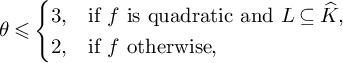 $$ \begin{align*}\theta \leqslant \begin{cases} 3, & \textrm {if }f\textrm{ is quadratic and }L\subseteq \widehat{K},\\ 2, & \textrm{if }f\textrm{ otherwise}, \end{cases} \end{align*} $$
where L denotes the number field generated by f.
If f is linear, then $\nu _f(p)=1$
for all
$\nu _f(p)=1$
for all $p\notin S$
, and so
$p\notin S$
, and so $\theta = \theta _0+ 1 = 2$
, as required. We now consider the case where f is an irreducible quadratic. Let
$\theta = \theta _0+ 1 = 2$
, as required. We now consider the case where f is an irreducible quadratic. Let
 $$ \begin{align*}\nu_f(p) = \#\{t \ (\mathrm{mod}\ p): f(t) \equiv 0 \ (\mathrm{mod}\ p)\}.\end{align*} $$
If $L\subseteq \widehat {K}$
, then Lemma 5.8 could be applied to compute
$L\subseteq \widehat {K}$
, then Lemma 5.8 could be applied to compute $\theta $
, with the desired error terms from (2.6). However, we apply the trivial bound
$\theta $
, with the desired error terms from (2.6). However, we apply the trivial bound $\nu _f(p)\leqslant 2$
for
$\nu _f(p)\leqslant 2$
for $p \notin S$
since it is not possible to improve on this in general. We therefore obtain
$p \notin S$
since it is not possible to improve on this in general. We therefore obtain $\theta \leqslant \theta _0+ 2 = 1+2 = 3$
, which is satisfactory.
$\theta \leqslant \theta _0+ 2 = 1+2 = 3$
, which is satisfactory.
We now assume that $L\not \subseteq \widehat {K}$
. We want to show that
$L\not \subseteq \widehat {K}$
. We want to show that $\theta =2$
, or equivalently that
$\theta =2$
, or equivalently that $\nu _f(p)=1$
on average over
$\nu _f(p)=1$
on average over $p \in \mathcal {P}$
. Let
$p \in \mathcal {P}$
. Let $M = \widehat {K}L$
be the compositum of
$M = \widehat {K}L$
be the compositum of $\widehat {K}$
and L. Since
$\widehat {K}$
and L. Since $\widehat {K}\cap L =\mathbb {Q}$
, we have by [Reference Lang34, Ch. VI, Theorem 1.14] that
$\widehat {K}\cap L =\mathbb {Q}$
, we have by [Reference Lang34, Ch. VI, Theorem 1.14] that $M/\mathbb {Q}$
is Galois, and
$M/\mathbb {Q}$
is Galois, and
 $$ \begin{align*}\mathrm{Gal}(M/\mathbb{Q}) \cong \mathrm{Gal}(L/\mathbb{Q}) \times \mathrm{Gal}(\widehat{K}/\mathbb{Q}) \cong \mathbb{Z}/2\mathbb{Z} \times \mathrm{Gal}(\widehat{K}/\mathbb{Q}).\end{align*} $$
We have $\nu _f(p) = 2$
if p is split in L, and
$\nu _f(p) = 2$
if p is split in L, and $\nu _f(p) = 0$
if p is inert in L, and so
$\nu _f(p) = 0$
if p is inert in L, and so
 $$ \begin{align} \theta = 1+ 2\lim_{x \rightarrow \infty}\left(\frac{\#\{p\leqslant x: p \in \mathcal{P}, \,p \textrm{ split in }L \}}{\#\{p\leqslant x: p \in \mathcal{P}\}}\right). \end{align} $$
Let $\sigma '=(\tau , \sigma )$
be an element of
$\sigma '=(\tau , \sigma )$
be an element of $\mathrm {Gal}(M/\mathbb {Q})$
, where
$\mathrm {Gal}(M/\mathbb {Q})$
, where $\tau \in \mathrm {Gal}(L/\mathbb {Q})$
and
$\tau \in \mathrm {Gal}(L/\mathbb {Q})$
and $\sigma \in \mathrm { Gal}(\widehat {K}/\mathbb {Q})$
. Applying Lemma 5.7, the primes
$\sigma \in \mathrm { Gal}(\widehat {K}/\mathbb {Q})$
. Applying Lemma 5.7, the primes $p\in \mathcal {P}$
correspond to the
$p\in \mathcal {P}$
correspond to the $\sigma '$
for which
$\sigma '$
for which $\sigma $
has non-coprime cycle lengths (so these primes have density
$\sigma $
has non-coprime cycle lengths (so these primes have density $T(G)$
as mentioned above). If in addition, the prime p is split in L, then we require that
$T(G)$
as mentioned above). If in addition, the prime p is split in L, then we require that $\tau = \textrm {id}$
. Therefore, by Lemma 5.8, asymptotically as
$\tau = \textrm {id}$
. Therefore, by Lemma 5.8, asymptotically as $x\rightarrow \infty $
, one half of the primes in
$x\rightarrow \infty $
, one half of the primes in $\mathcal {P}$
are also split in L. We conclude from (5.4) that (2.6) holds with
$\mathcal {P}$
are also split in L. We conclude from (5.4) that (2.6) holds with $\theta = 1+ 2(1/2) = 2$
.
$\theta = 1+ 2(1/2) = 2$
.
Proof of Theorem 1.3
We begin in the same manner as in the proof of Theorem 1.1, by appealing to Proposition 5.1 to reduce to a sieve problem. The binary form $F(x,y)$
has degree at most one higher than the degree of f. Therefore, we deduce from Theorem 2.3 that the Hasse principle holds for (1.1) provided that
$F(x,y)$
has degree at most one higher than the degree of f. Therefore, we deduce from Theorem 2.3 that the Hasse principle holds for (1.1) provided that $(\deg f +1)\sum _{j=1}^n \frac {1}{q_j-1}\leqslant 0.32380$
.
$(\deg f +1)\sum _{j=1}^n \frac {1}{q_j-1}\leqslant 0.32380$
.
Example 5.9. We consider the example $K=\mathbb {Q}(2^{1/q})$
discussed by Irving [Reference Irving27], where q is prime. Since K has prime degree, it satisfies the Hasse norm principle by work of Bartels [Reference Bartels1]. We now compute
$K=\mathbb {Q}(2^{1/q})$
discussed by Irving [Reference Irving27], where q is prime. Since K has prime degree, it satisfies the Hasse norm principle by work of Bartels [Reference Bartels1]. We now compute $G=\mathrm { Gal}(\widehat {K}/\mathbb {Q})$
. The minimum polynomial of
$G=\mathrm { Gal}(\widehat {K}/\mathbb {Q})$
. The minimum polynomial of $K/\mathbb {Q}$
is
$K/\mathbb {Q}$
is $x^q-2$
, which has roots
$x^q-2$
, which has roots $\{\beta , \beta \omega , \ldots , \beta \omega ^{q-1}\}$
, where
$\{\beta , \beta \omega , \ldots , \beta \omega ^{q-1}\}$
, where $\omega $
is a primitive qth root of unity and
$\omega $
is a primitive qth root of unity and $\beta $
is the real root of
$\beta $
is the real root of $x^q-2$
. We identify these roots with
$x^q-2$
. We identify these roots with $\{0,\ldots , q-1\}$
in the obvious way. An element
$\{0,\ldots , q-1\}$
in the obvious way. An element $\sigma \in G$
is determined by the image of
$\sigma \in G$
is determined by the image of $0$
and
$0$
and $1$
since
$1$
since $\beta , \beta \omega $
multiplicatively generate all the other roots. Therefore,
$\beta , \beta \omega $
multiplicatively generate all the other roots. Therefore, $\sigma $
takes the form
$\sigma $
takes the form $\sigma _{a,b}:x \mapsto ax+b$
for some
$\sigma _{a,b}:x \mapsto ax+b$
for some $a \in \mathbb {F}_q^{\times }, b \in \mathbb {F}_q$
. Conversely, the maps
$a \in \mathbb {F}_q^{\times }, b \in \mathbb {F}_q$
. Conversely, the maps $\sigma _{1,b}$
correspond to the q different embeddings K into
$\sigma _{1,b}$
correspond to the q different embeddings K into $\widehat {K}$
, and the maps
$\widehat {K}$
, and the maps $\sigma _{a,0}$
for
$\sigma _{a,0}$
for $a \in \mathbb {F}_q^{\times }$
are elements of
$a \in \mathbb {F}_q^{\times }$
are elements of $\mathrm {Gal}(\widehat {K}/K) \leqslant G$
. Combining these, we see that
$\mathrm {Gal}(\widehat {K}/K) \leqslant G$
. Combining these, we see that $\sigma _{a,b}\in G$
for any
$\sigma _{a,b}\in G$
for any $a \in \mathbb {F}_q^{\times }, b \in \mathbb {F}_q$
. We conclude that
$a \in \mathbb {F}_q^{\times }, b \in \mathbb {F}_q$
. We conclude that $G \cong \operatorname {AGL}(1,q)$
, the group of affine linear transformations on
$G \cong \operatorname {AGL}(1,q)$
, the group of affine linear transformations on $\mathbb {F}_q$
.
$\mathbb {F}_q$
.
When $a=1$
and
$a=1$
and $b\neq 0$
,
$b\neq 0$
, $\sigma _{a,b}$
is a q-cycle. For all other choices of
$\sigma _{a,b}$
is a q-cycle. For all other choices of $a,b$
, the equation
$a,b$
, the equation $ax+b=x$
has a solution
$ax+b=x$
has a solution $x \in \mathbb {F}_q$
, and so
$x \in \mathbb {F}_q$
, and so $\sigma _{a,b}$
has a fixed point. Therefore,
$\sigma _{a,b}$
has a fixed point. Therefore, $T(G) = (q-1)/\#G = 1/q$
. From this, we see that Irving’s choice of
$T(G) = (q-1)/\#G = 1/q$
. From this, we see that Irving’s choice of $\mathcal {P} = \{p \notin S: p \equiv 1 \ (\mathrm {mod}\ q)\}$
is not quite optimal,because it has density
$\mathcal {P} = \{p \notin S: p \equiv 1 \ (\mathrm {mod}\ q)\}$
is not quite optimal,because it has density $\alpha = 1/(q-1)$
, whereas the set of primes we actually need to sift out has density
$\alpha = 1/(q-1)$
, whereas the set of primes we actually need to sift out has density $T(G) = 1/q$
. In fact, we can see directly that even when
$T(G) = 1/q$
. In fact, we can see directly that even when $p\equiv 1 \ (\mathrm {mod}\ q)$
, there is sometimes a solution to
$p\equiv 1 \ (\mathrm {mod}\ q)$
, there is sometimes a solution to $x^q -2 \equiv 0 \ (\mathrm {mod}\ p)$
(e.g.,
$x^q -2 \equiv 0 \ (\mathrm {mod}\ p)$
(e.g., $q=3$
,
$q=3$
, $p = 31$
,
$p = 31$
, $x= 4$
). However, it can be checked that even with this smaller sieve dimension, we are still not able to handle the cases
$x= 4$
). However, it can be checked that even with this smaller sieve dimension, we are still not able to handle the cases $q=5$
or
$q=5$
or $q=3$
when f is an irreducible cubic.
$q=3$
when f is an irreducible cubic.
We remark that we can replace the number $2$
by any positive integer r such that
$2$
by any positive integer r such that $x^q-r$
is irreducible in the above example. (A necessary and sufficient condition for irreducibility of
$x^q-r$
is irreducible in the above example. (A necessary and sufficient condition for irreducibility of $x^q-r$
is given in [Reference Karpilovsky31, Theorem 8.16].) We can still take a sifting set
$x^q-r$
is given in [Reference Karpilovsky31, Theorem 8.16].) We can still take a sifting set $\mathcal {P}$
contained in
$\mathcal {P}$
contained in $\{p\notin S: p\equiv 1\ (\mathrm {mod}\ q)\}$
and with density
$\{p\notin S: p\equiv 1\ (\mathrm {mod}\ q)\}$
and with density $1/q$
, and the Galois group is still
$1/q$
, and the Galois group is still $\operatorname {AGL}(1,q)$
, and so generalising to
$\operatorname {AGL}(1,q)$
, and so generalising to $x^q-r$
does not affect the analysis.
$x^q-r$
does not affect the analysis.
5.4 Proof of Corollary 1.2
We now consider the case when $[K:\mathbb {Q}]=n$
and
$[K:\mathbb {Q}]=n$
and $G = S_n$
, with a view to proving Corollary 1.2. Such number fields automatically satisfy the Hasse principle by the work of Kunyavskiı̆ and Voskresenskiı̆ [32]. To ease notation, we shall write
$G = S_n$
, with a view to proving Corollary 1.2. Such number fields automatically satisfy the Hasse principle by the work of Kunyavskiı̆ and Voskresenskiı̆ [32]. To ease notation, we shall write $T(n)$
in place of
$T(n)$
in place of $T(S_n)$
. In the following lemma, we find an estimate for
$T(S_n)$
. In the following lemma, we find an estimate for $T(n)$
.
$T(n)$
.
Lemma 5.10. For all $n\geqslant 1$
, we have
$n\geqslant 1$
, we have
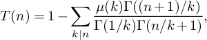 $$ \begin{align} T(n) &= 1-\sum_{k\mid n}\frac{\mu(k)\Gamma((n+1)/k)}{\Gamma(1/k)\Gamma(n/k+1)}, \end{align} $$
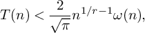 $$ \begin{align} T(n) &< \frac{2}{\sqrt{\pi}}n^{1/r-1}\omega(n), \end{align} $$
where r is the smallest prime factor of n and $\omega (n)$
is the number of prime factors of n.
$\omega (n)$
is the number of prime factors of n.
Proof. Define
 $$ \begin{align*}T_k(n) = \frac{1}{n!}\#\{\sigma \in S_n: \textrm{ the cycle lengths of }\sigma \textrm{ are all divisible by } k\}.\end{align*} $$
By Möbius inversion, we have $T(n) = 1-\sum _{k\mid n}\mu (k)T_k(n)$
. We now find an explicit formula for
$T(n) = 1-\sum _{k\mid n}\mu (k)T_k(n)$
. We now find an explicit formula for $T_k(n)$
. For
$T_k(n)$
. For $j\geqslant 1$
, let
$j\geqslant 1$
, let $a_{jk}$
denote the number of cycles of length
$a_{jk}$
denote the number of cycles of length $jk$
in
$jk$
in $\sigma $
. The cycle lengths of
$\sigma $
. The cycle lengths of $\sigma $
are all a multiple of k if and only if
$\sigma $
are all a multiple of k if and only if $\sum _{j=1}^{n/k} jka_{jk} = n$
. We apply the well-known formula for the number of permutations of
$\sum _{j=1}^{n/k} jka_{jk} = n$
. We apply the well-known formula for the number of permutations of $S_n$
with a given cycle shape to obtain
$S_n$
with a given cycle shape to obtain
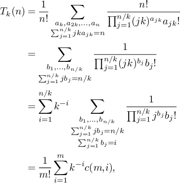 $$ \begin{align}T_k(n) &= \frac{1}{n!}\sum_{\substack{a_{k}, a_{2k}, \ldots, a_{n}\\ \sum_{j=1}^{n/k}jka_{jk}=n}}\frac{n!}{\prod_{j=1}^{n/k}(jk)^{a_{jk}}a_{jk}!}\nonumber\\ &=\sum_{\substack{b_1,\ldots, b_{n/k}\\ \sum_{j=1}^{n/k}jb_j=n/k}}\frac{1}{\prod_{j=1}^{n/k}(jk)^{b_j}b_j!}\nonumber\\ &=\sum_{i=1}^{n/k}k^{-i}\sum_{\substack{b_1, \ldots, b_{n/k}\\ \sum_{j=1}^{n/k}jb_j=n/k\\ \sum_{j=1}^{n/k}b_j = i}}\frac{1}{\prod_{j=1}^{n/k}j^{b_j}b_j!}\nonumber\\ &= \frac{1}{m!}\sum_{i = 1}^{m}k^{-i}c(m,i), \end{align} $$
where $m = n/k$
and
$m = n/k$
and $c(m,i)$
is the number of
$c(m,i)$
is the number of $\sigma ' \in S_m$
with exactly i cycles. The quantity
$\sigma ' \in S_m$
with exactly i cycles. The quantity $c(m,i)$
is called the Stirling number of the first kind. In order to evaluate (5.7), we follow the argument from [Reference Flajolet and Sedgewick17, Example II.12]. We define a bivariate generating function
$c(m,i)$
is called the Stirling number of the first kind. In order to evaluate (5.7), we follow the argument from [Reference Flajolet and Sedgewick17, Example II.12]. We define a bivariate generating function
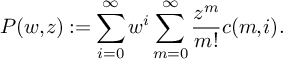
By [Reference Flajolet and Sedgewick17, Proposition II.4], we have
 $$ \begin{align*}\sum_{m=0}^{\infty}\frac{z^m}{m!}c(m,i) = \frac{1}{i!}\left(\log\left(\frac{1}{1-z}\right)\right)^i.\end{align*} $$
Therefore,
 $$ \begin{align*}P(w,z) = \sum_{i=0}^{\infty}\frac{w^i}{i!}\left(\log\left(\frac{1}{1-z}\right)\right)^i = \exp\left(w\log\left(\frac{1}{1-z}\right)\right)=(1-z)^{-w}.\end{align*} $$
Applying the Binomial theorem, we find that the $z^m$
coefficient of
$z^m$
coefficient of $P(w,z)$
is equal to
$P(w,z)$
is equal to $w(w+1)\cdots (w+m-1)/m!$
. However, if we substitute
$w(w+1)\cdots (w+m-1)/m!$
. However, if we substitute $w= 1/k$
, the
$w= 1/k$
, the $z^m$
coefficient of (5.8) is precisely (5.7). We conclude that
$z^m$
coefficient of (5.8) is precisely (5.7). We conclude that
 $$ \begin{align*} \frac{1}{m!}\sum_{i=1}^m k^{-i}c(m,i) &= (1/k)(1+1/k)\cdots (m-1+1/k)/m!\\ &=\frac{\Gamma(m+1/k)}{\Gamma(1/k)\Gamma(m+1)}, \end{align*} $$
which completes the proof of (5.5).
We now establish the upper bound in (5.6). A basic bound on the gamma function is that for any real $s\in (0,1)$
and any positive real number x, we have
$s\in (0,1)$
and any positive real number x, we have
 $$ \begin{align*}x^{1-s} < \frac{\Gamma(x+1)}{\Gamma(x+s)} < (1+x)^{1-s}.\end{align*} $$
Applying this with $x=m$
and
$x=m$
and $s=1/k$
, we have
$s=1/k$
, we have
 $$ \begin{align*}\frac{\Gamma(m + 1/k)}{\Gamma(m+1)}< m^{1/k - 1}.\end{align*} $$
Moreover, we have
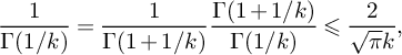 $$ \begin{align*}\frac{1}{\Gamma(1/k)} = \frac{1}{\Gamma(1+1/k)}\frac{\Gamma(1+1/k)}{\Gamma(1/k)}\leqslant \frac{2}{\sqrt{\pi}k},\end{align*} $$
since $\Gamma (1+1/k)$
for integers
$\Gamma (1+1/k)$
for integers $k\geqslant 2$
achieves its minimum at
$k\geqslant 2$
achieves its minimum at $k=2$
, where we have
$k=2$
, where we have $\Gamma (1+1/k)=\Gamma (3/2) = \sqrt {\pi }/2$
. We conclude that
$\Gamma (1+1/k)=\Gamma (3/2) = \sqrt {\pi }/2$
. We conclude that
 $$ \begin{align*}T_k(n)< \frac{2}{\sqrt{\pi}k}(n/k)^{1/k-1}= \frac{2}{\sqrt{\pi}}n^{1/k-1}k^{-1/k}<\frac{2}{\sqrt{\pi}}n^{1/k-1}.\end{align*} $$
Taking a sum over $k=p$
prime, we obtain
$k=p$
prime, we obtain
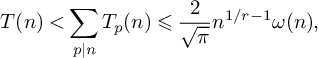 $$ \begin{align*}T(n) < \sum_{p\mid n}T_p(n) \leqslant \frac{2}{\sqrt{\pi}}n^{1/r-1}\omega(n),\end{align*} $$
as required.
Proof of Corollary 1.2
We recall the setting of Corollary 1.2. We assume that $G=S_n$
, and f is a product of two quadratics generating a biquadratic extension L of
$G=S_n$
, and f is a product of two quadratics generating a biquadratic extension L of $\mathbb {Q}$
. We apply Theorem 2.1 to the binary form
$\mathbb {Q}$
. We apply Theorem 2.1 to the binary form $\prod _{i=0}^2 f_i(x,y)$
, where
$\prod _{i=0}^2 f_i(x,y)$
, where $f_0(x,y) = y$
and
$f_0(x,y) = y$
and $f_1(x,y), f_2(x,y)$
are the homogenisations of the two quadratic factors of f. We also assume that
$f_1(x,y), f_2(x,y)$
are the homogenisations of the two quadratic factors of f. We also assume that $L\cap \widehat {K} = \mathbb {Q}$
, and so by the proof of Theorem 1.1, we have
$L\cap \widehat {K} = \mathbb {Q}$
, and so by the proof of Theorem 1.1, we have $\theta _0= \theta _1 = \theta _2 = 1$
, and
$\theta _0= \theta _1 = \theta _2 = 1$
, and $\theta = 3$
. By maximising the value of
$\theta = 3$
. By maximising the value of $\kappa $
in (4.55) directly, we find by numerical computations that the largest value of
$\kappa $
in (4.55) directly, we find by numerical computations that the largest value of $\kappa $
we can take here is
$\kappa $
we can take here is $0.42214\ldots $
. (The slight improvement over
$0.42214\ldots $
. (The slight improvement over $\kappa \leqslant 0.39$
for the general case comes from computing
$\kappa \leqslant 0.39$
for the general case comes from computing $\alpha \sum _{i=m+1}^k \theta _i = 2\alpha $
in our example, whilst in the proof of Theorem 1.1, we applied the trivial bound
$\alpha \sum _{i=m+1}^k \theta _i = 2\alpha $
in our example, whilst in the proof of Theorem 1.1, we applied the trivial bound $\alpha \sum _{i=m+1}^k \theta _i \leqslant \kappa = 3\alpha $
.) Hence, the Hasse principle holds for
$\alpha \sum _{i=m+1}^k \theta _i \leqslant \kappa = 3\alpha $
.) Hence, the Hasse principle holds for $f(t) = \mathbf {N}(\mathbf {x})\neq 0$
provided that
$f(t) = \mathbf {N}(\mathbf {x})\neq 0$
provided that $T(n) \leqslant 0.42214\ldots /3 = 0.14071\ldots $
.
$T(n) \leqslant 0.42214\ldots /3 = 0.14071\ldots $
.
We use the upper bound (5.6) from Lemma 5.10 to reduce the n for which $T(n)\geqslant 0.14071\ldots $
to finitely many cases, and then the exact formula (5.5) to find precisely which n satisfy
$T(n)\geqslant 0.14071\ldots $
to finitely many cases, and then the exact formula (5.5) to find precisely which n satisfy $T(n)\geqslant 0.14071\ldots $
. We find that
$T(n)\geqslant 0.14071\ldots $
. We find that $T(n)\leqslant 0.14071\ldots $
unless
$T(n)\leqslant 0.14071\ldots $
unless $n\in \{2,3,\ldots , 10, 12,14,15,16,18,20,22,24,26,28,30,36,42,48\}.$
6 Application to the Harpaz–Wittenberg conjecture
In this section, we apply the sieve result from Theorem 2.1 to prove Theorem 1.4. We recall the statement of [Reference Harpaz and Wittenberg23, Conjecture 9.1] (we shall only work with the ground field $\mathbb {Q}$
).
$\mathbb {Q}$
).
Conjecture 6.1 (Harpaz, Wittenberg)
Let $P_1, \ldots , P_n \in \mathbb {Q}[t]$
be pairwise distinct irreducible monic polynomials. Let
$P_1, \ldots , P_n \in \mathbb {Q}[t]$
be pairwise distinct irreducible monic polynomials. Let $k_i=\mathbb {Q}[t]/(P_i(t))$
be the corresponding number fields. Let
$k_i=\mathbb {Q}[t]/(P_i(t))$
be the corresponding number fields. Let $a_i\in k_i$
denote the class of t. For each
$a_i\in k_i$
denote the class of t. For each $i\in \{1,\ldots , n\}$
, let
$i\in \{1,\ldots , n\}$
, let $L_i/k_i$
be a finite extension, and let
$L_i/k_i$
be a finite extension, and let $b_i \in k_i^*$
. Let
$b_i \in k_i^*$
. Let $S_0$
be a finite set of places of
$S_0$
be a finite set of places of $\mathbb {Q}$
including the archimedean place, and all finite places above which, for some i, either
$\mathbb {Q}$
including the archimedean place, and all finite places above which, for some i, either $b_i$
is not a unit or
$b_i$
is not a unit or $L_i/k_i$
is ramified. For each
$L_i/k_i$
is ramified. For each $v\in S_0$
, fix an element
$v\in S_0$
, fix an element $t_v \in \mathbb {Q}_v$
. Suppose that for every
$t_v \in \mathbb {Q}_v$
. Suppose that for every $i\in \{1,\ldots , n\}$
and every
$i\in \{1,\ldots , n\}$
and every $v\in S_0$
, there exists
$v\in S_0$
, there exists $x_{i,v} \in (L_i \otimes _{\mathbb {Q}} \mathbb {Q}_v)^*$
such that
$x_{i,v} \in (L_i \otimes _{\mathbb {Q}} \mathbb {Q}_v)^*$
such that $b_i(t_v-a_i) = N_{L_i\otimes _{\mathbb {Q}} \mathbb {Q}_v/k_i \otimes _{\mathbb {Q}} \mathbb {Q}_v}(x_{i,v})$
in
$b_i(t_v-a_i) = N_{L_i\otimes _{\mathbb {Q}} \mathbb {Q}_v/k_i \otimes _{\mathbb {Q}} \mathbb {Q}_v}(x_{i,v})$
in $k_i \otimes _{\mathbb {Q}} \mathbb {Q}_v$
. Then there exists
$k_i \otimes _{\mathbb {Q}} \mathbb {Q}_v$
. Then there exists $t_0 \in \mathbb {Q}$
satisfying the following conditions.
$t_0 \in \mathbb {Q}$
satisfying the following conditions.
-
(1)
$t_0$
is arbitrarily close to
$t_v$
for all
$v \in S_0$
. -
(2) For every
$i\in \{1,\ldots , n\}$
and every place
$\mathfrak {p}$
of
$k_i$
with
$\operatorname {ord}_{\mathfrak {p}}(t_0-a_i)>0$
, either
$\mathfrak {p}$
lies above a place of
$S_0$
or the field
$L_i$
possesses a place of degree
$1$
over
$\mathfrak {p}$
.


We remark that below, the $b_i$
and
$b_i$
and $x_{i,v}$
appearing in Conjecture 6.1 do not play a role, and so in the cases that Theorem 1.4 applies, it establishes a stronger version of Conjecture 6.1, where the assumption on the existence of the elements
$x_{i,v}$
appearing in Conjecture 6.1 do not play a role, and so in the cases that Theorem 1.4 applies, it establishes a stronger version of Conjecture 6.1, where the assumption on the existence of the elements $x_{i,v}$
is removed. We discuss this further in Section 6.1.
$x_{i,v}$
is removed. We discuss this further in Section 6.1.
We can reduce Conjecture 6.1 to a sieve problem as follows. Let $f_i(x,y) = c_iN_{k_i/\mathbb {Q}}(x-a_iy)$
, where
$f_i(x,y) = c_iN_{k_i/\mathbb {Q}}(x-a_iy)$
, where $c_i \in \mathbb {Q}$
is chosen such that the coefficients of
$c_i \in \mathbb {Q}$
is chosen such that the coefficients of $f_i(x,y)$
are coprime integers. Then
$f_i(x,y)$
are coprime integers. Then $f_i(x,y)$
is an irreducible polynomial in
$f_i(x,y)$
is an irreducible polynomial in $\mathbb {Z}[x,y]$
.
$\mathbb {Z}[x,y]$
.
Below, we suppose that S is a finite set of primes containing all primes in $S_0$
and all primes dividing any of the denominators
$S_0$
and all primes dividing any of the denominators $c_1, \ldots , c_n$
. For
$c_1, \ldots , c_n$
. For $i\in \{1,\ldots , n\}$
, we define
$i\in \{1,\ldots , n\}$
, we define $\mathcal {P}_i$
to be the set of primes
$\mathcal {P}_i$
to be the set of primes $p \notin S$
, such that for some place
$p \notin S$
, such that for some place $\mathfrak {p}$
of
$\mathfrak {p}$
of $k_i$
above p,
$k_i$
above p, $L_i$
does not possess a place of degree
$L_i$
does not possess a place of degree $1$
above
$1$
above $\mathfrak {p}$
.
$\mathfrak {p}$
.
Lemma 6.2. Let $k_1, \ldots , k_n$
and
$k_1, \ldots , k_n$
and $L_1, \ldots , L_n$
and
$L_1, \ldots , L_n$
and $S_0$
be as in Conjecture 6.1, and let
$S_0$
be as in Conjecture 6.1, and let $\mathcal {P}_i$
and
$\mathcal {P}_i$
and $f_i(x,y)$
be as defined above. Suppose that there exists a finite set of primes
$f_i(x,y)$
be as defined above. Suppose that there exists a finite set of primes $S\supset S_0\backslash \{\infty \}$
such that for any congruence condition
$S\supset S_0\backslash \{\infty \}$
such that for any congruence condition $C(x,y)$
on
$C(x,y)$
on $x,y$
modulo an integer
$x,y$
modulo an integer $\Delta $
with only prime factors in S, and any real numbers
$\Delta $
with only prime factors in S, and any real numbers $r, \xi>0$
, there exists
$r, \xi>0$
, there exists $x_0,y_0 \in \mathbb {N}$
such that
$x_0,y_0 \in \mathbb {N}$
such that
-
(i)
$C(x_0,y_0)$
holds, -
(ii)
$|x_0/y_0 - r| < \xi $
, -
(iii)
$f_i(x_0,y_0)$
has no prime factors in
$\mathcal {P}_i$
for all
$i\in \{1, \ldots , n\}$
.


Then Conjecture 6.1 holds for this choice of $k_1,\ldots ,k_n,L_1, \ldots , L_n$
and
$k_1,\ldots ,k_n,L_1, \ldots , L_n$
and $S_0$
.
$S_0$
.
Proof. From [Reference Harpaz and Wittenberg23, Remark 9.3 (iii)], we are free to adjoin to $S_0$
a finite number of places, and so we may assume that
$S_0$
a finite number of places, and so we may assume that $S_0 = S\cup \{\infty \}$
. We may assume that the value
$S_0 = S\cup \{\infty \}$
. We may assume that the value $t_{\infty }$
prescribed in Conjecture 6.1 is non-negative, and let
$t_{\infty }$
prescribed in Conjecture 6.1 is non-negative, and let $t_0 = x_0/y_0$
. (If alternatively
$t_0 = x_0/y_0$
. (If alternatively $t_{\infty } < 0$
, then we instead choose
$t_{\infty } < 0$
, then we instead choose $t_0 = -x_0/y_0$
and proceed similarly.) Then property (1) of Conjecture 6.1 immediately follows from (i) and (ii) by appropriate choices of
$t_0 = -x_0/y_0$
and proceed similarly.) Then property (1) of Conjecture 6.1 immediately follows from (i) and (ii) by appropriate choices of $C(x,y), r$
and
$C(x,y), r$
and $\xi $
. Let
$\xi $
. Let $\mathfrak {p}$
be a place of
$\mathfrak {p}$
be a place of $k_i$
above a prime
$k_i$
above a prime $p \notin S$
, satisfying
$p \notin S$
, satisfying $\operatorname {ord}_{\mathfrak {p}}(t_0-a_i)>0$
. Then
$\operatorname {ord}_{\mathfrak {p}}(t_0-a_i)>0$
. Then
 $$ \begin{align*}f_i(x_0,y_0) = y_0^{\deg f_i} f_i(x_0/y_0,1) = y_0^{\deg f_i}c_i N_{k_i/\mathbb{Q}}(t_0-a_i).\end{align*} $$
Now $\operatorname {ord}_{\mathfrak {p}}(t_0-a_i)>0$
implies that
$\operatorname {ord}_{\mathfrak {p}}(t_0-a_i)>0$
implies that $\operatorname {ord}_p(N_{k_i/\mathbb {Q}}(t_0-a_i))>0$
. Since
$\operatorname {ord}_p(N_{k_i/\mathbb {Q}}(t_0-a_i))>0$
. Since $p \notin S$
, we have
$p \notin S$
, we have $\operatorname {ord}_p(y_0c_i) \geqslant 0$
, and so
$\operatorname {ord}_p(y_0c_i) \geqslant 0$
, and so $p\mid f_i(x_0,y_0)$
. By (iii), we have
$p\mid f_i(x_0,y_0)$
. By (iii), we have $p \notin \mathcal {P}_i$
, and so by construction of
$p \notin \mathcal {P}_i$
, and so by construction of $\mathcal {P}_i$
, we deduce that property (2) of Conjecture 6.1 holds.
$\mathcal {P}_i$
, we deduce that property (2) of Conjecture 6.1 holds.
In view of Lemma 6.2, we let
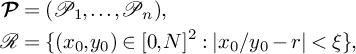
and we aim to show that the sifting function
is positive for sufficiently large N. We do not attempt here to generalise Theorem 2.1 to deal with different sifting sets $\mathcal {P}_i$
for each i, but instead define below in (6.14) a set
$\mathcal {P}_i$
for each i, but instead define below in (6.14) a set $\mathcal {P} \supseteq \bigcup _{i=1}^n \mathcal {P}_i$
and replace each of the conditions
$\mathcal {P} \supseteq \bigcup _{i=1}^n \mathcal {P}_i$
and replace each of the conditions $\gcd (f_i(x_0,y_0), P_i(x))=1$
with
$\gcd (f_i(x_0,y_0), P_i(x))=1$
with $\gcd (f_i(x_0,y_0), P(x))=1$
.
$\gcd (f_i(x_0,y_0), P(x))=1$
.
Proof of Theorem 1.4
We recall that $L_i$
is the compositum
$L_i$
is the compositum $k_iM_i$
, for a number field
$k_iM_i$
, for a number field $M_i$
which is linearly disjoint to
$M_i$
which is linearly disjoint to $k_i$
over
$k_i$
over $\mathbb {Q}$
. Consequently,
$\mathbb {Q}$
. Consequently, $[L_i:k_i] = [M_i:\mathbb {Q}]$
. Writing
$[L_i:k_i] = [M_i:\mathbb {Q}]$
. Writing $M_i = \mathbb {Q}(\beta _i)$
using the primitive element theorem, we therefore have that the minimum polynomial of
$M_i = \mathbb {Q}(\beta _i)$
using the primitive element theorem, we therefore have that the minimum polynomial of $\beta _i$
over
$\beta _i$
over $\mathbb {Q}$
and over
$\mathbb {Q}$
and over $k_i$
coincide. We denote this minimum polynomial by
$k_i$
coincide. We denote this minimum polynomial by $g_i$
.
$g_i$
.
Let $\mathfrak {p}$
denote a place of
$\mathfrak {p}$
denote a place of $k_i$
. For all but finitely many places, the inertia degrees of the places of
$k_i$
. For all but finitely many places, the inertia degrees of the places of $L_i$
above
$L_i$
above $\mathfrak {p}$
are the degrees of
$\mathfrak {p}$
are the degrees of $g_i$
when factored modulo
$g_i$
when factored modulo $\mathfrak {p}$
. If
$\mathfrak {p}$
. If $g_i$
has a root modulo p, then it has a root modulo every
$g_i$
has a root modulo p, then it has a root modulo every $\mathfrak {p}\mid p$
, and so
$\mathfrak {p}\mid p$
, and so $p \notin \mathcal {P}_i$
. Therefore, for suitably chosen S, we have
$p \notin \mathcal {P}_i$
. Therefore, for suitably chosen S, we have
Define $\mathcal {P} = \bigcup _{i=1}^n \widetilde {\mathcal {P}}_i$
. Clearly, to show that the sifting function
$\mathcal {P} = \bigcup _{i=1}^n \widetilde {\mathcal {P}}_i$
. Clearly, to show that the sifting function ![]() from (6.1) is positive, it suffices to show the sifting function
from (6.1) is positive, it suffices to show the sifting function $S(\mathcal {A}, \mathcal {P},x)$
(in the notation of (4.2)) is positive.
$S(\mathcal {A}, \mathcal {P},x)$
(in the notation of (4.2)) is positive.
By the Chebotarev density theorem (Lemma 5.8), the sets $\widetilde {\mathcal {P}_i}$
have density
$\widetilde {\mathcal {P}_i}$
have density $\alpha _i = T_i$
, where
$\alpha _i = T_i$
, where $T_i$
is defined in (1.4). The sets
$T_i$
is defined in (1.4). The sets $\widetilde {\mathcal {P}_i}$
are examples of Frobenian sets as defined by Serre [Reference Serre41, Section 3.3.1], which roughly means that away from S their membership is determined Artin symbols of some Galois extension (here
$\widetilde {\mathcal {P}_i}$
are examples of Frobenian sets as defined by Serre [Reference Serre41, Section 3.3.1], which roughly means that away from S their membership is determined Artin symbols of some Galois extension (here $\widehat {M_i}$
). It follows from [Reference Serre41, Proposition 3.7 b)] that the intersection of Frobenian sets is Frobenian. Since
$\widehat {M_i}$
). It follows from [Reference Serre41, Proposition 3.7 b)] that the intersection of Frobenian sets is Frobenian. Since $\mathcal {P}$
is a disjoint union of such intersections, we conclude from Theorem 5.5 that the set
$\mathcal {P}$
is a disjoint union of such intersections, we conclude from Theorem 5.5 that the set $\mathcal {P}$
does indeed have a density. We shall bound its density trivially by
$\mathcal {P}$
does indeed have a density. We shall bound its density trivially by $\sum _{i=1}^n \alpha _i$
.
$\sum _{i=1}^n \alpha _i$
.
We now bound the value of $\theta $
defined in (2.6). Here, we have already defined
$\theta $
defined in (2.6). Here, we have already defined $f_i$
to be a binary form, and so no additional term
$f_i$
to be a binary form, and so no additional term $\theta _0$
coming from homogenisation is required. We apply the trivial estimate
$\theta _0$
coming from homogenisation is required. We apply the trivial estimate $\nu _i(p) \leqslant \deg f_i = [k_i:\mathbb {Q}]$
for all
$\nu _i(p) \leqslant \deg f_i = [k_i:\mathbb {Q}]$
for all $p \notin S$
. We conclude that
$p \notin S$
. We conclude that $\theta \leqslant \sum _{i=1}^n[k_i:\mathbb {Q}]=d$
. Combining Lemma 6.2 and Theorem 2.1 completes the proof of part (1) of Theorem 1.4.
$\theta \leqslant \sum _{i=1}^n[k_i:\mathbb {Q}]=d$
. Combining Lemma 6.2 and Theorem 2.1 completes the proof of part (1) of Theorem 1.4.
We now turn to the cubic case. Assumption 2.2 holds for our choice $\mathcal {P}$
and f. As in Section 4.8, we conclude that
$\mathcal {P}$
and f. As in Section 4.8, we conclude that ![]() for sufficiently large N, provided that
for sufficiently large N, provided that $t\leqslant 0.32380$
, where
$t\leqslant 0.32380$
, where $t = \deg f \sum _{i=1}^n 1/(q_i-1)$
. Rearranging, and recalling
$t = \deg f \sum _{i=1}^n 1/(q_i-1)$
. Rearranging, and recalling $\deg f=d$
, we complete the proof of part (2) of Theorem 1.4.
$\deg f=d$
, we complete the proof of part (2) of Theorem 1.4.
Remark 6.3. In contrast to Section 5, now $\mathrm {Gal}(\widehat {M_i}/\mathbb {Q})=S_n$
is not a case we can handle because there the proportion of fixed point free elements is
$\mathrm {Gal}(\widehat {M_i}/\mathbb {Q})=S_n$
is not a case we can handle because there the proportion of fixed point free elements is $1-1/e$
as
$1-1/e$
as $n\rightarrow \infty $
(where
$n\rightarrow \infty $
(where $e=2.718\ldots $
is Euler’s constant), which is much too large.
$e=2.718\ldots $
is Euler’s constant), which is much too large.
For a permutation group G acting on $X=\{1, \ldots , k\}$
, we define
$X=\{1, \ldots , k\}$
, we define $h(G)$
to be the proportion of elements of G with no fixed point. The family of of groups G for which
$h(G)$
to be the proportion of elements of G with no fixed point. The family of of groups G for which $h(G)$
is smallest are the Frobenius groups. These are the groups where G has a nontrivial element fixing one point of X, but no nontrivial elements fixing more than one point of X. We state two known results about Frobenius groups.
$h(G)$
is smallest are the Frobenius groups. These are the groups where G has a nontrivial element fixing one point of X, but no nontrivial elements fixing more than one point of X. We state two known results about Frobenius groups.
Lemma 6.4 [Reference Sonn43, Theorem 1]
Any Frobenius group can be realised as a Galois group over $\mathbb {Q}$
.
$\mathbb {Q}$
.
Lemma 6.5 [Reference Boston, Dabrowski, Foguel, Gies, Jackson, Ose and Walker3, Theorem 3.1]
Let G be a transitive permutation group on k letters.
-
(1) We have
$h(G) \geqslant 1/k$
, with equality if and only if G is a Frobenius group of order
$k(k-1)$
and k is a prime power. -
(2) In all other cases,
$h(G) \geqslant 2/k$
.


Proof of Corollary 1.5
As computed in Example 5.9, we have that $G_i :=\mathrm {Gal}(\widehat {M_i}/\mathbb {Q})$
is isomorphic to the group
$G_i :=\mathrm {Gal}(\widehat {M_i}/\mathbb {Q})$
is isomorphic to the group $\operatorname {AGL}(1,q_i)$
of affine linear transformations on
$\operatorname {AGL}(1,q_i)$
of affine linear transformations on $\mathbb {F}_{q_i}$
. This is a Frobenius group of order
$\mathbb {F}_{q_i}$
. This is a Frobenius group of order $q_i(q_i-1)$
. By Lemma 6.5, we have
$q_i(q_i-1)$
. By Lemma 6.5, we have $T_i = h(G_i) = 1/q_i$
. (This also agrees with our computation in Example 5.9.) If
$T_i = h(G_i) = 1/q_i$
. (This also agrees with our computation in Example 5.9.) If $[k_i:\mathbb {Q}]\leqslant 2$
for all i, we can therefore apply part (1) of Theorem 1.4 provided that
$[k_i:\mathbb {Q}]\leqslant 2$
for all i, we can therefore apply part (1) of Theorem 1.4 provided that $\sum _{i=1}^n 1/q_i \leqslant 0.39/d$
. Moreover, for all
$\sum _{i=1}^n 1/q_i \leqslant 0.39/d$
. Moreover, for all $i\in \{1,\ldots , n\}$
, the sifting sets
$i\in \{1,\ldots , n\}$
, the sifting sets $\mathcal {P}_i$
are contained in
$\mathcal {P}_i$
are contained in $\{p\notin S: p \equiv 1 \ (\mathrm {mod}\ q_i)\}$
. Indeed, when
$\{p\notin S: p \equiv 1 \ (\mathrm {mod}\ q_i)\}$
. Indeed, when $p \not \equiv 1 \ (\mathrm {mod}\ q_i)$
, the qth power map on
$p \not \equiv 1 \ (\mathrm {mod}\ q_i)$
, the qth power map on $\mathbb {F}_p^{\times }$
is a bijection, and so
$\mathbb {F}_p^{\times }$
is a bijection, and so $x^{q_i}-r_i$
has a root modulo p.
$x^{q_i}-r_i$
has a root modulo p.
The minimum polynomial $x^{q_i}-r_i$
has a root modulo p for all but finitely many
$x^{q_i}-r_i$
has a root modulo p for all but finitely many $p \not \equiv 1 \ (\mathrm {mod}\ q_i)$
, and these finitely many exceptional primes can be included in
$p \not \equiv 1 \ (\mathrm {mod}\ q_i)$
, and these finitely many exceptional primes can be included in $S_0$
. Therefore, we can apply part (2) of Theorem 1.4 provided that
$S_0$
. Therefore, we can apply part (2) of Theorem 1.4 provided that $\sum _{i=1}^n 1/(q_i-1) \leqslant 0.32380/d$
.
$\sum _{i=1}^n 1/(q_i-1) \leqslant 0.32380/d$
.
6.1 The hypothesis on
$b_i$

Given that the quantities $b_i$
play no role in Theorem 1.4, it is natural to ask under what circumstances we should expect a stronger version of Conjecture 6.1 to hold, without the hypothesis on the
$b_i$
play no role in Theorem 1.4, it is natural to ask under what circumstances we should expect a stronger version of Conjecture 6.1 to hold, without the hypothesis on the $b_i$
. The following proposition demonstrates that the hypothesis remains unchanged after passing to maximal abelian subextensions of each
$b_i$
. The following proposition demonstrates that the hypothesis remains unchanged after passing to maximal abelian subextensions of each $L_i/k_i$
.
$L_i/k_i$
.
Proposition 6.6. Let $L/k$
be an extension of number fields. Let
$L/k$
be an extension of number fields. Let $L'/k$
be the maximal abelian subextension of
$L'/k$
be the maximal abelian subextension of $L/k$
. Let S be a sufficiently large set of places of k, including all archimedean places. For each
$L/k$
. Let S be a sufficiently large set of places of k, including all archimedean places. For each $v\in S$
, fix an element
$v\in S$
, fix an element $b_v \in k_v^{*}$
. Then the following are equivalent:
$b_v \in k_v^{*}$
. Then the following are equivalent:
-
(1) There exists an S-unit
$b \in k$
such that for all
$v\in S$
,
$b/b_v$
is in the image of the norm map
$(L\otimes _k k_v)^* \rightarrow k_v^*$
. -
(2) There exists an S-unit
$b \in k$
such that for all
$v\in S$
,
$b/b_v$
is in the image of the norm map
$(L'\otimes _k k_v)^* \rightarrow k_v^*$
.


We prove Proposition 6.6 at the end of this section. We now demonstrate how the lack of the hypothesis on $b_i$
in Theorem 1.4 is explained by Proposition 6.6. We shall choose S to consist of all places that lie above a finite set of places
$b_i$
in Theorem 1.4 is explained by Proposition 6.6. We shall choose S to consist of all places that lie above a finite set of places $S_0$
of k, which corresponds to the set
$S_0$
of k, which corresponds to the set $S_0$
from Conjecture 6.1. We recall that due to [Reference Harpaz and Wittenberg23, Remark 9.3 (iii)], we are free to make
$S_0$
from Conjecture 6.1. We recall that due to [Reference Harpaz and Wittenberg23, Remark 9.3 (iii)], we are free to make $S_0$
, and hence S, large enough that Proposition 6.6 applies. We apply Proposition 6.6 with
$S_0$
, and hence S, large enough that Proposition 6.6 applies. We apply Proposition 6.6 with $L=L_i$
and
$L=L_i$
and $k=k_i$
for each extension
$k=k_i$
for each extension $L_i/k_i$
from Conjecture 6.1, and with
$L_i/k_i$
from Conjecture 6.1, and with $b_v = 1/(t_v-a_i)$
. Clearly, if
$b_v = 1/(t_v-a_i)$
. Clearly, if $L/k$
contains no nontrivial abelian subextensions (so that
$L/k$
contains no nontrivial abelian subextensions (so that $L'=k$
), then Condition (2) above is trivially satisfied, and so Proposition 6.6 implies that the hypothesis on
$L'=k$
), then Condition (2) above is trivially satisfied, and so Proposition 6.6 implies that the hypothesis on $b_i$
in Conjecture 6.1 is vacuous. To complete the argument, it suffices to show that in the setting of Theorem 1.4, we have
$b_i$
in Conjecture 6.1 is vacuous. To complete the argument, it suffices to show that in the setting of Theorem 1.4, we have $L_i^{\prime } = k_i$
for all i. In fact, in the following lemma, we show that the hypotheses of Theorem 1.4 force the stronger property that the
$L_i^{\prime } = k_i$
for all i. In fact, in the following lemma, we show that the hypotheses of Theorem 1.4 force the stronger property that the $L_i/k_i$
contain no nontrivial Galois subextensions.
$L_i/k_i$
contain no nontrivial Galois subextensions.
Lemma 6.7. Suppose that $L/k$
is one of the extensions
$L/k$
is one of the extensions $L_i/k_i$
from Theorem 1.4, and let
$L_i/k_i$
from Theorem 1.4, and let $T=T_i$
be as in (1.4). Suppose that
$T=T_i$
be as in (1.4). Suppose that $T[k:\mathbb {Q}]< 1/2$
. Then
$T[k:\mathbb {Q}]< 1/2$
. Then $L/k$
has no nontrivial Galois subextensions.
$L/k$
has no nontrivial Galois subextensions.
Proof. We recall from the proof of Theorem 1.4 that $T\geqslant \alpha $
, where
$T\geqslant \alpha $
, where $\alpha $
is the natural density of the set
$\alpha $
is the natural density of the set $\mathcal {P}$
of primes
$\mathcal {P}$
of primes $p\notin S$
such that there is some place
$p\notin S$
such that there is some place $\mathfrak {p}$
of k above p for which L does not possess a place of degree 1 above
$\mathfrak {p}$
of k above p for which L does not possess a place of degree 1 above $\mathfrak {p}$
. For
$\mathfrak {p}$
. For $x\geqslant 1$
, we have the trivial bound
$x\geqslant 1$
, we have the trivial bound
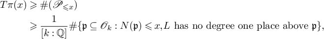 $$ \begin{align*}T\pi(x) &\geqslant \#(\mathcal{P}_{\leqslant x})\\ &\geqslant \frac{1}{[k:\mathbb{Q}]}\#\{\mathfrak{p} \subseteq \mathcal{O}_k: N(\mathfrak{p})\leqslant x, L \textrm{ has no degree one place above }\mathfrak{p}\}, \end{align*} $$
since there are at most $[k:\mathbb {Q}]$
prime ideals
$[k:\mathbb {Q}]$
prime ideals $\mathfrak {p}$
above each p, and
$\mathfrak {p}$
above each p, and $N(\mathfrak {p})\geqslant p$
.
$N(\mathfrak {p})\geqslant p$
.
Suppose that $N/k$
is a Galois subextension of
$N/k$
is a Galois subextension of $L/k$
. In order for L to possess a degree one place above
$L/k$
. In order for L to possess a degree one place above $\mathfrak {p}$
, so must N. However, since
$\mathfrak {p}$
, so must N. However, since $N/k$
is Galois, N possesses a place of degree one above
$N/k$
is Galois, N possesses a place of degree one above $\mathfrak {p}$
if and only in
$\mathfrak {p}$
if and only in $\mathfrak {p}$
splits completely in N, and by the Chebotarev density theorem, this occurs with density
$\mathfrak {p}$
splits completely in N, and by the Chebotarev density theorem, this occurs with density $1/[N:k]$
. We deduce that
$1/[N:k]$
. We deduce that
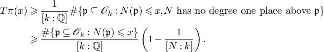 $$ \begin{align*}T\pi(x)&\geqslant \frac{1}{[k:\mathbb{Q}]}\#\{\mathfrak{p} \subseteq \mathcal{O}_k: N(\mathfrak{p})\leqslant x, N \textrm{ has no degree one place above }\mathfrak{p}\}\\ &\geqslant \frac{\#\{\mathfrak{p} \subseteq \mathcal{O}_k: N(\mathfrak{p}) \leqslant x\}}{[k:\mathbb{Q}]}\left(1-\frac{1}{[N:k]}\right). \end{align*} $$
Taking a limit at $x\rightarrow \infty $
and applying the prime ideal theorem, we conclude that
$x\rightarrow \infty $
and applying the prime ideal theorem, we conclude that
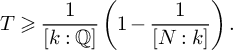 $$ \begin{align*}T\geqslant \frac{1}{[k:\mathbb{Q}]}\left(1-\frac{1}{[N:k]}\right).\end{align*} $$
The assumption $T[k:\mathbb {Q}]<1/2$
therefore implies that
$T[k:\mathbb {Q}]<1/2$
therefore implies that $N=k$
.
$N=k$
.
Let T denote the norm one torus associated to $L/k$
, which is the algebraic group over k defined by the the equation
$L/k$
, which is the algebraic group over k defined by the the equation $\mathbf {N}_{L/k}(\mathbf {x}) = 1$
. We have a short exact sequence
$\mathbf {N}_{L/k}(\mathbf {x}) = 1$
. We have a short exact sequence
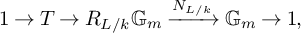 $$ \begin{align} 1 \rightarrow T \rightarrow R_{L/k}\mathbb{G}_m \xrightarrow{N_{L/k}} \mathbb{G}_m \rightarrow 1, \end{align} $$
where $R_{L/k}$
denotes the Weil restriction. Let
$R_{L/k}$
denotes the Weil restriction. Let $T_{\overline {k}} = T\times _k \overline {k}$
and
$T_{\overline {k}} = T\times _k \overline {k}$
and $\mathbb {G}_{m,\overline {k}}\cong \overline {k}^{\times }$
. We define the character group of T to be
$\mathbb {G}_{m,\overline {k}}\cong \overline {k}^{\times }$
. We define the character group of T to be $\widehat {T} = \operatorname {Hom}(T_{\overline {k}},\mathbb {G}_{m,\overline {k}})$
, viewed as a Galois module via the natural action of
$\widehat {T} = \operatorname {Hom}(T_{\overline {k}},\mathbb {G}_{m,\overline {k}})$
, viewed as a Galois module via the natural action of $\mathrm {Gal}(\overline {k}/k)$
.
$\mathrm {Gal}(\overline {k}/k)$
.
Let $\mathcal {O}_{S}$
denote the ring of S-integers of k, and
$\mathcal {O}_{S}$
denote the ring of S-integers of k, and $\mathcal {O}_{L, S_L}$
the ring of
$\mathcal {O}_{L, S_L}$
the ring of $S_L$
-integers of L, where
$S_L$
-integers of L, where $S_L$
consists of all places of L above a place in S. We include in S all places of k which ramify in L. Then
$S_L$
consists of all places of L above a place in S. We include in S all places of k which ramify in L. Then $\mathcal {O}_{L,S_L}/\mathcal {O}_{S}$
is étale, and so the equation
$\mathcal {O}_{L,S_L}/\mathcal {O}_{S}$
is étale, and so the equation $\mathbf {N}_{\mathcal {O}_{L,S_L}/\mathcal {O}_{S}}(\mathbf {z}) = 1$
defines a model
$\mathbf {N}_{\mathcal {O}_{L,S_L}/\mathcal {O}_{S}}(\mathbf {z}) = 1$
defines a model $\mathcal {T}$
of T over
$\mathcal {T}$
of T over $\mathcal {O}_S$
. Similarly to (6.3), we have a short exact sequence
$\mathcal {O}_S$
. Similarly to (6.3), we have a short exact sequence
 $$ \begin{align} 1 \rightarrow \mathcal{T} \rightarrow R_{\mathcal{O}_{L,S_L}/\mathcal{O}_S}\mathbb{G}_{m,\mathcal{O}_{L,S_L}} \xrightarrow{N_{L/k}} \mathbb{G}_{m,\mathcal{O}_S} \rightarrow 1. \end{align} $$
Let $k_S$
denote the maximal subextension of
$k_S$
denote the maximal subextension of $\overline {k}/k$
which is unramified at all places not contained in S. Below, we shall work with profinite group cohomology of
$\overline {k}/k$
which is unramified at all places not contained in S. Below, we shall work with profinite group cohomology of ![]() . We note that L is a subextension of
. We note that L is a subextension of $k_S$
since S is assumed to contain all ramified places of
$k_S$
since S is assumed to contain all ramified places of $L/k$
. We may therefore define
$L/k$
. We may therefore define $G_{L,S} = \mathrm {Gal}(k_S/L)$
. Let
$G_{L,S} = \mathrm {Gal}(k_S/L)$
. Let $A_S$
denote the integral closure of
$A_S$
denote the integral closure of $\mathcal {O}_S$
in
$\mathcal {O}_S$
in $k_S$
. The natural action of
$k_S$
. The natural action of $\mathrm {Gal}(\overline {k}/k)$
on
$\mathrm {Gal}(\overline {k}/k)$
on $\widehat {T}$
factors through
$\widehat {T}$
factors through $G_S$
, so
$G_S$
, so $\widehat {T}$
can be viewed as a
$\widehat {T}$
can be viewed as a $G_S$
-module. The character group
$G_S$
-module. The character group $\operatorname {Hom}(\mathcal {T}_{A_S}, \mathbb {G}_{m, A_S})$
is nothing more than
$\operatorname {Hom}(\mathcal {T}_{A_S}, \mathbb {G}_{m, A_S})$
is nothing more than $\widehat {T}$
as a
$\widehat {T}$
as a $G_S$
-module, so we shall henceforth denote it by
$G_S$
-module, so we shall henceforth denote it by $\widehat {T}$
.
$\widehat {T}$
.
Lemma 6.8. Let $\varphi :H^1(G_S, \mathbb {Q}/\mathbb {Z}) \rightarrow H^1(G_{L,S},\mathbb {Q}/\mathbb {Z})$
be the restriction map induced by the inclusion
$\varphi :H^1(G_S, \mathbb {Q}/\mathbb {Z}) \rightarrow H^1(G_{L,S},\mathbb {Q}/\mathbb {Z})$
be the restriction map induced by the inclusion $G_{L,S} \hookrightarrow G_S$
. Then there is an exact sequence
$G_{L,S} \hookrightarrow G_S$
. Then there is an exact sequence
 $$ \begin{align} 0 \rightarrow H^1(G_S,\widehat{T}) \rightarrow H^1(G_S,\mathbb{Q}/\mathbb{Z}) \xrightarrow{\varphi} H^1(G_{L,S},\mathbb{Q}/\mathbb{Z}). \end{align} $$
Proof. We begin by taking character groups of the short exact sequence (6.4), or in other words, applying the contravariant functor $\operatorname {Hom}(-, \mathbb {G}_{m,A_S})$
. we obtain a short exact sequence
$\operatorname {Hom}(-, \mathbb {G}_{m,A_S})$
. we obtain a short exact sequence
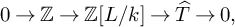 $$ \begin{align} 0 \rightarrow \mathbb{Z} \rightarrow \mathbb{Z}[L/k] \rightarrow \widehat{T} \rightarrow 0, \end{align} $$
where $\mathbb {Z}[L/k]\cong \mathbb {Z}[\mathcal {O}_{L,S_L}/\mathcal {O}_{S}]$
denotes the free abelian group generated by the k-linear embeddings
$\mathbb {Z}[L/k]\cong \mathbb {Z}[\mathcal {O}_{L,S_L}/\mathcal {O}_{S}]$
denotes the free abelian group generated by the k-linear embeddings $L\hookrightarrow \overline {k}$
. We now take group cohomology of (6.6) to obtain a long exact sequence
$L\hookrightarrow \overline {k}$
. We now take group cohomology of (6.6) to obtain a long exact sequence
 $$ \begin{align} \cdots \rightarrow H^1(G_S,\mathbb{Z}[L/k]) \rightarrow H^1(G_S,\widehat{T}) \rightarrow H^2(G_S,\mathbb{Z}) \rightarrow H^2(G_S,\mathbb{Z}[L/k]) \rightarrow \cdots. \end{align} $$
For any groups $H\leqslant G$
, any H-module N and any integer
$H\leqslant G$
, any H-module N and any integer $i\geqslant 0$
, Shapiro’s lemma [Reference Milne37, Proposition 1.11] states that
$i\geqslant 0$
, Shapiro’s lemma [Reference Milne37, Proposition 1.11] states that $H^i(H,N)\cong H^i(G,\operatorname {Coind}^G_H(N))$
, where
$H^i(H,N)\cong H^i(G,\operatorname {Coind}^G_H(N))$
, where $\operatorname {Coind}^G_H(N) = \operatorname {Hom}_{\mathbb {Z}[H]}(\mathbb {Z}[G],N)$
denotes the coinduced module. We apply Shapiro’s lemma to the first and last terms in the exact sequence (6.7) by choosing
$\operatorname {Coind}^G_H(N) = \operatorname {Hom}_{\mathbb {Z}[H]}(\mathbb {Z}[G],N)$
denotes the coinduced module. We apply Shapiro’s lemma to the first and last terms in the exact sequence (6.7) by choosing $G=G_S, H=G_{L,S}$
and
$G=G_S, H=G_{L,S}$
and $N=\mathbb {Z}$
. Then
$N=\mathbb {Z}$
. Then
 $$ \begin{align*}\operatorname{Coind}^G_H(N) = \operatorname{Hom}_{\mathbb{Z}[G_{L,S}]}(\mathbb{Z}[G_S],\mathbb{Z})\cong \mathbb{Z}[G_S/G_{L,S}] \cong \mathbb{Z}[L/k],\end{align*} $$
and so we conclude that $H^i(G_S,\mathbb {Z}[L/k]) \cong H^i(G_{L,S},\mathbb {Z})$
for all
$H^i(G_S,\mathbb {Z}[L/k]) \cong H^i(G_{L,S},\mathbb {Z})$
for all $i\geqslant 0$
. Moreover,
$i\geqslant 0$
. Moreover, $H^1(G_{L,S},\mathbb {Z})$
consists of all continuous group homomorphisms
$H^1(G_{L,S},\mathbb {Z})$
consists of all continuous group homomorphisms $G_{L,S} \rightarrow \mathbb {Z}$
. Since
$G_{L,S} \rightarrow \mathbb {Z}$
. Since $G_{L,S}$
is compact, and
$G_{L,S}$
is compact, and $\mathbb {Z}$
is discrete, we have
$\mathbb {Z}$
is discrete, we have $H^1(G_{L,S},\mathbb {Z}) = 0$
. Therefore, we obtain from (6.7) the exact sequence
$H^1(G_{L,S},\mathbb {Z}) = 0$
. Therefore, we obtain from (6.7) the exact sequence
 $$ \begin{align} 0 \rightarrow H^1(G_S,\widehat{T}) \rightarrow H^2(G_S,\mathbb{Z}) \rightarrow H^2(G_{L,S},\mathbb{Z}). \end{align} $$
Now, for any subextension E of $k_S/k$
, we have
$k_S/k$
, we have $H^2(G_{E,S},\mathbb {Z}) \cong H^1(G_{E,S}, \mathbb {Q}/\mathbb {Z})$
. To see this, we take group cohomology of the exact sequence
$H^2(G_{E,S},\mathbb {Z}) \cong H^1(G_{E,S}, \mathbb {Q}/\mathbb {Z})$
. To see this, we take group cohomology of the exact sequence $0 \rightarrow \mathbb {Z} \rightarrow \mathbb {Q} \rightarrow \mathbb {Q}/\mathbb {Z} \rightarrow 0$
to obtain a long exact sequence
$0 \rightarrow \mathbb {Z} \rightarrow \mathbb {Q} \rightarrow \mathbb {Q}/\mathbb {Z} \rightarrow 0$
to obtain a long exact sequence
 $$ \begin{align*} \cdots \rightarrow H^1(G_{E,S},\mathbb{Q}) \rightarrow H^1(G_{E,S}, \mathbb{Q}/\mathbb{Z}) \rightarrow H^2(G_{E,S},\mathbb{Z}) \rightarrow H^2(G_{E,S},\mathbb{Q}) \rightarrow \cdots, \end{align*} $$
and note that $H^1(G_{E,S},\mathbb {Q}) = H^2(G_{E,S},\mathbb {Q}) = 0$
since
$H^1(G_{E,S},\mathbb {Q}) = H^2(G_{E,S},\mathbb {Q}) = 0$
since $G_{E,S}$
is a profinite group [Reference Neukirch, Schmidt and Wingberg39, Proposition 1.6.2 (c)]. Therefore, applying this fact with
$G_{E,S}$
is a profinite group [Reference Neukirch, Schmidt and Wingberg39, Proposition 1.6.2 (c)]. Therefore, applying this fact with $E=k$
and
$E=k$
and $E=L$
, we have an exact sequence
$E=L$
, we have an exact sequence
 $$ \begin{align} 0 \rightarrow H^1(G_S,\widehat{T}) \rightarrow H^1(G_S,\mathbb{Q}/\mathbb{Z}) \xrightarrow{\psi} H^1(G_{L,S},\mathbb{Q}/\mathbb{Z}). \end{align} $$
To complete the proof, we need to show that the map $\psi $
we have obtained from the above argument is equal to the map
$\psi $
we have obtained from the above argument is equal to the map $\varphi $
defined in the lemma. We consider the diagram
$\varphi $
defined in the lemma. We consider the diagram
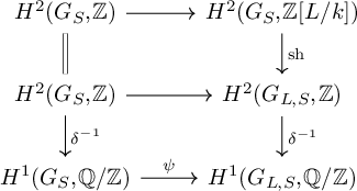
Here, $\delta ^{-1}$
denotes the inverse of the connecting homomorphism, and
$\delta ^{-1}$
denotes the inverse of the connecting homomorphism, and $\operatorname {sh}$
denotes the Shapiro map, (i.e., the isomorphism from the above application of Shapiro’s lemma). By definition,
$\operatorname {sh}$
denotes the Shapiro map, (i.e., the isomorphism from the above application of Shapiro’s lemma). By definition, $\psi $
comes from applying these isomorphisms to the map
$\psi $
comes from applying these isomorphisms to the map $H^2(G_S, \mathbb {Z}) \rightarrow H^2(G_S,\mathbb {Z}[L/k])$
from (6.7), which is the map
$H^2(G_S, \mathbb {Z}) \rightarrow H^2(G_S,\mathbb {Z}[L/k])$
from (6.7), which is the map $i_*$
in the notation of [Reference Neukirch, Schmidt and Wingberg39, Proposition 1.6.5]. Therefore, by [Reference Neukirch, Schmidt and Wingberg39, Proposition 1.6.5], the middle horizontal arrow is just the restriction map. Finally, restriction maps commute with connecting homomorphisms [Reference Neukirch, Schmidt and Wingberg39, Proposition 1.5.2], and so
$i_*$
in the notation of [Reference Neukirch, Schmidt and Wingberg39, Proposition 1.6.5]. Therefore, by [Reference Neukirch, Schmidt and Wingberg39, Proposition 1.6.5], the middle horizontal arrow is just the restriction map. Finally, restriction maps commute with connecting homomorphisms [Reference Neukirch, Schmidt and Wingberg39, Proposition 1.5.2], and so $\psi $
is the restriction homomorphism induced by the inclusion
$\psi $
is the restriction homomorphism induced by the inclusion $G_{L,S} \hookrightarrow G_S$
, as required.
$G_{L,S} \hookrightarrow G_S$
, as required.
In what follows, we denote by $\operatorname {Cl}_{S_L}(L)$
the
$\operatorname {Cl}_{S_L}(L)$
the $S_L$
-ideal class group (i.e., the quotient of the usual class group
$S_L$
-ideal class group (i.e., the quotient of the usual class group $\operatorname {Cl}(L)$
by the classes of all prime ideals in
$\operatorname {Cl}(L)$
by the classes of all prime ideals in $S_L$
). Since
$S_L$
). Since $\operatorname {Cl}(L)$
is finite, by adjoining finitely many primes to S, we may assume that
$\operatorname {Cl}(L)$
is finite, by adjoining finitely many primes to S, we may assume that $\operatorname {Cl}_{S_L}(L)=0$
.
$\operatorname {Cl}_{S_L}(L)=0$
.
Lemma 6.9. Let S be as above. If $a\in k^*$
lies in the image of the norm map
$a\in k^*$
lies in the image of the norm map $(k_v\otimes _k L)^* \rightarrow k_v^*$
for all
$(k_v\otimes _k L)^* \rightarrow k_v^*$
for all $v\notin S$
, then there exists
$v\notin S$
, then there exists $y\in N_{L/k}(L^*)$
such that
$y\in N_{L/k}(L^*)$
such that $ay \in \mathcal {O}_S^{\times }$
.
$ay \in \mathcal {O}_S^{\times }$
.
Proof. Fix a place $v\notin S$
at which a is not a unit. Let
$v\notin S$
at which a is not a unit. Let $w_1\cdots w_r$
be the factorisation of v into prime ideals in
$w_1\cdots w_r$
be the factorisation of v into prime ideals in $\mathcal {O}_L$
, and let
$\mathcal {O}_L$
, and let $c_i = [L_{w_i}: k_v]$
be the corresponding inertia degrees. (Since
$c_i = [L_{w_i}: k_v]$
be the corresponding inertia degrees. (Since $L/k$
is unramified outside S, the ideals
$L/k$
is unramified outside S, the ideals $w_1, \ldots , w_r$
are distinct.) We define
$w_1, \ldots , w_r$
are distinct.) We define $c=\gcd (c_1, \ldots , c_r)$
. The image of the norm map
$c=\gcd (c_1, \ldots , c_r)$
. The image of the norm map $(k_v\otimes _k L)^* \rightarrow k_v^*$
consists of the elements of
$(k_v\otimes _k L)^* \rightarrow k_v^*$
consists of the elements of $k_v^*$
whose valuation is divisible by c. In particular, we may write
$k_v^*$
whose valuation is divisible by c. In particular, we may write $v(a) = \sum _{i=1}^r n_ic_i$
for some integers
$v(a) = \sum _{i=1}^r n_ic_i$
for some integers $n_1, \ldots , n_r$
. Since
$n_1, \ldots , n_r$
. Since $\operatorname {Cl}_{S_L}(L)=0$
, we can find an element
$\operatorname {Cl}_{S_L}(L)=0$
, we can find an element $z_v\in L$
such that
$z_v\in L$
such that $w_i(z_v) = n_i$
for all
$w_i(z_v) = n_i$
for all $i\in \{1,\ldots , r\}$
, and such that
$i\in \{1,\ldots , r\}$
, and such that $z_v$
is a unit at all other places not in
$z_v$
is a unit at all other places not in $S_L$
. Let
$S_L$
. Let $y_v = N_{L/k}(z_v)$
. Then
$y_v = N_{L/k}(z_v)$
. Then $v(y_v) = \sum _{i=1}^r n_i c_i = v(a)$
, and
$v(y_v) = \sum _{i=1}^r n_i c_i = v(a)$
, and $y_v$
is a unit at all other places outside S. The result now follows by taking y to be the product of the elements
$y_v$
is a unit at all other places outside S. The result now follows by taking y to be the product of the elements $y_v^{-1}$
over the (finitely many) places
$y_v^{-1}$
over the (finitely many) places $v\notin S$
at which a is not a unit.
$v\notin S$
at which a is not a unit.
Proof of Proposition 6.6
The implication $(1)\implies (2)$
is trivial, so we only need to prove
$(1)\implies (2)$
is trivial, so we only need to prove $(2)\implies (1)$
. Taking Galois cohomology of (6.3), we obtain a long exact sequence
$(2)\implies (1)$
. Taking Galois cohomology of (6.3), we obtain a long exact sequence
 $$ \begin{align} 1 \rightarrow T(k) \rightarrow L^{\times} \xrightarrow{N_{L/k}} k^{\times} \xrightarrow{\delta_k} H^1(k,T)\rightarrow H^1(k,R_{L/k}\mathbb{G}_m)\rightarrow \cdots. \end{align} $$
Hilbert’s Theorem 90 [Reference Colliot-Thélène and Skorobogatov11, Theorem 1.3.2] implies that $H^1(k,R_{L/k}\mathbb {G}_m)$
is trivial, and so we can naturally identify
$H^1(k,R_{L/k}\mathbb {G}_m)$
is trivial, and so we can naturally identify $H^1(k,T)$
with
$H^1(k,T)$
with $\frac {k^{\times }}{N_{L/k}(L^{\times })}$
. In a similar way, we can identify
$\frac {k^{\times }}{N_{L/k}(L^{\times })}$
. In a similar way, we can identify $H^1(k_v, T)$
with the quotient of
$H^1(k_v, T)$
with the quotient of $k_v^*$
by the image of the norm map
$k_v^*$
by the image of the norm map $(L\otimes _k k_v)^* \rightarrow k_v^*$
. We can also take group cohomology of the short exact sequence (6.4) to obtain a long exact sequence
$(L\otimes _k k_v)^* \rightarrow k_v^*$
. We can also take group cohomology of the short exact sequence (6.4) to obtain a long exact sequence
 $$ \begin{align} 1 \rightarrow \mathcal{T}(\mathcal{O}_{S}) \rightarrow \mathcal{O}_{L,S_L}^{\times} \rightarrow \mathcal{O}_{S}^{\times} \xrightarrow{\delta_{\mathcal{O}_S}} H^1(G_S,\mathcal{T}_{A_S}) \rightarrow H^1(G_S, A_{S_L}^{\times}) \rightarrow \cdots, \end{align} $$
where $A_{S_L} = A_S \otimes _{\mathcal {O}_S} \mathcal {O}_{L, S_L}$
is the integral closure of
$A_{S_L} = A_S \otimes _{\mathcal {O}_S} \mathcal {O}_{L, S_L}$
is the integral closure of $\mathcal {O}_{L,S_L}$
in
$\mathcal {O}_{L,S_L}$
in $k_S$
. (We remark that the ring
$k_S$
. (We remark that the ring $A_S$
is denoted by
$A_S$
is denoted by $\mathcal {O}_S$
in [Reference Neukirch, Schmidt and Wingberg39].) By [Reference Neukirch, Schmidt and Wingberg39, Proposition 8.3.11 (ii)], we have
$\mathcal {O}_S$
in [Reference Neukirch, Schmidt and Wingberg39].) By [Reference Neukirch, Schmidt and Wingberg39, Proposition 8.3.11 (ii)], we have $H^1(G_S, A_{S_L}^{\times }) \cong \operatorname {Cl}_{S_L}(L)$
, which we recall is trivial due to our choice of S. Therefore, we may identify
$H^1(G_S, A_{S_L}^{\times }) \cong \operatorname {Cl}_{S_L}(L)$
, which we recall is trivial due to our choice of S. Therefore, we may identify $H^1(G_S, \mathcal {T}_{A_S})$
with
$H^1(G_S, \mathcal {T}_{A_S})$
with $\frac {\mathcal {O}_{S}^{\times }}{\mathcal {O}_{S}^{\times } \cap N_{L/k}(L^{\times })}$
.
$\frac {\mathcal {O}_{S}^{\times }}{\mathcal {O}_{S}^{\times } \cap N_{L/k}(L^{\times })}$
.
Let $v\in S$
, and let
$v\in S$
, and let $\overline {k}_v$
denote an algebraic closure of
$\overline {k}_v$
denote an algebraic closure of $k_v$
. Fixing an embedding
$k_v$
. Fixing an embedding $k_S \hookrightarrow \overline {k_v}$
determines a surjection
$k_S \hookrightarrow \overline {k_v}$
determines a surjection $\mathrm {Gal}(\overline {k_v}/k_v) \rightarrow G_S$
, which induces restriction maps
$\mathrm {Gal}(\overline {k_v}/k_v) \rightarrow G_S$
, which induces restriction maps $H^1(G_S, \mathcal {T}_{A_S}) \rightarrow H^1(k_v, T)$
and
$H^1(G_S, \mathcal {T}_{A_S}) \rightarrow H^1(k_v, T)$
and $H^1(k, T) \rightarrow H^1(k_v, T)$
called localisation maps. Below, we denote these maps by
$H^1(k, T) \rightarrow H^1(k_v, T)$
called localisation maps. Below, we denote these maps by $\operatorname {res}_v$
. Under the above identifications, we obtain a commutative diagram
$\operatorname {res}_v$
. Under the above identifications, we obtain a commutative diagram
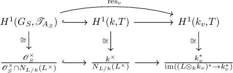
where $(L \otimes _k k_v)^* \rightarrow k_v^*$
denotes the norm map, and the bottom arrows are induced by the inclusions
$(L \otimes _k k_v)^* \rightarrow k_v^*$
denotes the norm map, and the bottom arrows are induced by the inclusions $\mathcal {O}_S^{\times } \hookrightarrow k \hookrightarrow k_v^*$
. Consequently, we can reformulate Condition (1) from Proposition 6.6 as
$\mathcal {O}_S^{\times } \hookrightarrow k \hookrightarrow k_v^*$
. Consequently, we can reformulate Condition (1) from Proposition 6.6 as
-
(3) The class of
$(b_v)_{v \in S}$
in
$\prod _{v \in S}H^1(k_v, T)$
belongs to the image of the map
$\prod _{v \in S}\operatorname {res}_v$
.


We assume that S is also large enough that $\operatorname {Cl}_{S_{L'}}(L')=0$
, so that the above argument gives a similar reformulation of (2), but with the torus
$\operatorname {Cl}_{S_{L'}}(L')=0$
, so that the above argument gives a similar reformulation of (2), but with the torus $T'$
associated to
$T'$
associated to $L'/k$
in place of T.
$L'/k$
in place of T.
Let $(-)^{\vee }=\operatorname {Hom}(-,\mathbb {Q}/\mathbb {Z})$
. Poitou–Tate duality [Reference Neukirch, Schmidt and Wingberg39, Theorem 4.20 b)] gives an exact sequence
$(-)^{\vee }=\operatorname {Hom}(-,\mathbb {Q}/\mathbb {Z})$
. Poitou–Tate duality [Reference Neukirch, Schmidt and Wingberg39, Theorem 4.20 b)] gives an exact sequence
 $$ \begin{align} H^1(k,T) \xrightarrow{\operatorname{res}} \sideset{}{'}\prod H^1(k_v, T) \xrightarrow{\xi} H^1(k, \widehat{T})^{\vee}. \end{align} $$
Here, the restricted product is over all places v of k, with the added assumption that the specified element of $H^1(k_v,T)$
comes from
$H^1(k_v,T)$
comes from $H^1(\mathcal {O}_v, T)$
for all but finitely many v, and the first map is induced by the residue maps
$H^1(\mathcal {O}_v, T)$
for all but finitely many v, and the first map is induced by the residue maps $\operatorname {res}_v$
for each place v of k.
$\operatorname {res}_v$
for each place v of k.
Let $\iota : \prod _{v\in S}H^1(k_v, T) \hookrightarrow \sideset {}{'}\prod H^1(k_v, T)$
be defined by adding trivial classes at the places
$\iota : \prod _{v\in S}H^1(k_v, T) \hookrightarrow \sideset {}{'}\prod H^1(k_v, T)$
be defined by adding trivial classes at the places $v\notin S$
, and let
$v\notin S$
, and let $\xi _S = \xi \circ \iota $
. We now explain how to deduce from (6.13) an exact sequence of the form
$\xi _S = \xi \circ \iota $
. We now explain how to deduce from (6.13) an exact sequence of the form
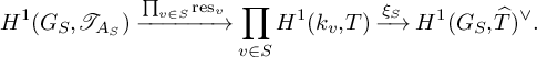 $$ \begin{align} H^1(G_S, \mathcal{T}_{A_S}) \xrightarrow{\prod_{v\in S}\operatorname{res}_v} \prod_{v \in S}H^1(k_v,T) \xrightarrow{\xi_S} H^1(G_S,\widehat{T})^{\vee}. \end{align} $$
Suppose that $b= (b_v)_{v\in S} \in \ker (\xi _S)$
. Then
$b= (b_v)_{v\in S} \in \ker (\xi _S)$
. Then $\iota (b) \in \ker \xi $
. By the exactness of (6.13), this implies
$\iota (b) \in \ker \xi $
. By the exactness of (6.13), this implies $\iota (b) =\operatorname {res}(a)$
for some
$\iota (b) =\operatorname {res}(a)$
for some $a\in H^1(k,T)$
. Moreover, we know that
$a\in H^1(k,T)$
. Moreover, we know that $\operatorname {res}_v(a)$
is trivial at all places
$\operatorname {res}_v(a)$
is trivial at all places $v\notin S$
. Recalling the identifications from (6.12), this means that a lies in the image of the norm map
$v\notin S$
. Recalling the identifications from (6.12), this means that a lies in the image of the norm map $(k_v \otimes _L k)^* \rightarrow k_v^*$
for all
$(k_v \otimes _L k)^* \rightarrow k_v^*$
for all $v\notin S$
. By Lemma 6.9, there is a representative of the class
$v\notin S$
. By Lemma 6.9, there is a representative of the class $a\in H^1(k,T)$
which is contained in
$a\in H^1(k,T)$
which is contained in $\mathcal {O}_S^{\times }$
. Therefore, a in fact lies in
$\mathcal {O}_S^{\times }$
. Therefore, a in fact lies in $H^1(G_S, \mathcal {T}_{A_S})$
. It follows that
$H^1(G_S, \mathcal {T}_{A_S})$
. It follows that $\prod _{v\in S}\operatorname {res}_v(a) = b$
, establishing the exactness of (6.14). Hence, condition (1) from the proposition is equivalent to the condition
$\prod _{v\in S}\operatorname {res}_v(a) = b$
, establishing the exactness of (6.14). Hence, condition (1) from the proposition is equivalent to the condition $(b_v)_{v\in S} \in \ker \xi _S$
.
$(b_v)_{v\in S} \in \ker \xi _S$
.
The map $\xi _S$
is induced by the localisation maps
$\xi _S$
is induced by the localisation maps $\prod _{v \in S}\operatorname {res}_v:H^1(G_S, \widehat {T}) \rightarrow \prod _{v\in S}H^1(k_v,\widehat {T})$
and the pairing
$\prod _{v \in S}\operatorname {res}_v:H^1(G_S, \widehat {T}) \rightarrow \prod _{v\in S}H^1(k_v,\widehat {T})$
and the pairing
 $$ \begin{align*}\prod_{v\in S}\left(H^1(k_v,T)\times H^1(k_v,\widehat{T})\right)\xrightarrow{\cup}\prod_{v\in S}H^2(k_v, \mathbb{G}_m)\xrightarrow{\sum_{v \in S}\operatorname{inv}_v} \mathbb{Q}/\mathbb{Z},\end{align*} $$
where $\cup $
denotes the cup product applied at each place
$\cup $
denotes the cup product applied at each place $v\in S$
and
$v\in S$
and $\operatorname {inv}_v$
denotes the local invariant map, as defined in [Reference Neukirch, Schmidt and Wingberg39, pp. 156].
$\operatorname {inv}_v$
denotes the local invariant map, as defined in [Reference Neukirch, Schmidt and Wingberg39, pp. 156].
Consider the diagram
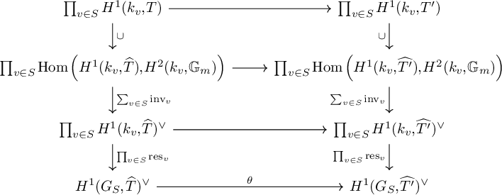
where all the horizontal arrows are induced by the map $T\xrightarrow {N_{L/L'}} T'$
. (The norm map
$T\xrightarrow {N_{L/L'}} T'$
. (The norm map $N_{L/L'}: R_{L/k}\mathbb {G}_m \rightarrow R_{L'/k}\mathbb {G}_m$
restricts to a map
$N_{L/L'}: R_{L/k}\mathbb {G}_m \rightarrow R_{L'/k}\mathbb {G}_m$
restricts to a map $T \rightarrow T'$
because
$T \rightarrow T'$
because $N_{L/k}(z) = N_{L/L'}(N_{L'/k}(z))$
for any
$N_{L/k}(z) = N_{L/L'}(N_{L'/k}(z))$
for any $z \in L$
.) This diagram commutes, thanks to the functorality properties of the localisation maps
$z \in L$
.) This diagram commutes, thanks to the functorality properties of the localisation maps $\operatorname {res}_v$
[Reference Neukirch, Schmidt and Wingberg39, Proposition 1.5.2], and the projection formula for the cup product [Reference Neukirch, Schmidt and Wingberg39, Proposition 1.4.2]. The composition of the vertical arrows are the map
$\operatorname {res}_v$
[Reference Neukirch, Schmidt and Wingberg39, Proposition 1.5.2], and the projection formula for the cup product [Reference Neukirch, Schmidt and Wingberg39, Proposition 1.4.2]. The composition of the vertical arrows are the map $\xi _S$
and the corresponding map
$\xi _S$
and the corresponding map $\xi ^{\prime }_{S}$
for
$\xi ^{\prime }_{S}$
for $T'$
. Therefore, we obtain a commutative diagram
$T'$
. Therefore, we obtain a commutative diagram
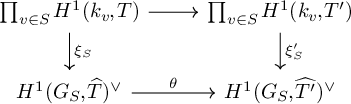
Applying Lemma 6.8, we have $H^1(G_S,\widehat {T}) \cong \ker \varphi $
, where
$H^1(G_S,\widehat {T}) \cong \ker \varphi $
, where $\varphi $
is as defined in the exact sequence (6.5). As discussed in the paragraphs preceding Lemma A.5,
$\varphi $
is as defined in the exact sequence (6.5). As discussed in the paragraphs preceding Lemma A.5, $\varphi $
sends cyclic subextensions
$\varphi $
sends cyclic subextensions $M/k$
of
$M/k$
of $k_S$
(with a given choice of generator for
$k_S$
(with a given choice of generator for $\mathrm {Gal}(M/k)$
) to their compositum
$\mathrm {Gal}(M/k)$
) to their compositum $LM/L$
, and so elements of
$LM/L$
, and so elements of $\ker \varphi $
correspond to cyclic subextensions of
$\ker \varphi $
correspond to cyclic subextensions of $L/k$
. However, since
$L/k$
. However, since $L'/k$
is the maximal abelian subextension of
$L'/k$
is the maximal abelian subextension of $L/k$
, it contains all cyclic subextensions of
$L/k$
, it contains all cyclic subextensions of $L/k$
, and so the map
$L/k$
, and so the map $H^1(G_S, \widehat {T'}) \rightarrow H^1(G_S, \widehat {T})$
is surjective. Since
$H^1(G_S, \widehat {T'}) \rightarrow H^1(G_S, \widehat {T})$
is surjective. Since $\mathbb {Q}/\mathbb {Z}$
is a divisible group, it is an injective object in the category of abelian groups, and so the contravariant functor
$\mathbb {Q}/\mathbb {Z}$
is a divisible group, it is an injective object in the category of abelian groups, and so the contravariant functor $\operatorname {Hom}(-,\mathbb {Q}/\mathbb {Z})$
is exact. We deduce that
$\operatorname {Hom}(-,\mathbb {Q}/\mathbb {Z})$
is exact. We deduce that $\theta $
is an injection. Therefore, if
$\theta $
is an injection. Therefore, if $\xi ^{\prime }_S((b_v)_{v\in S})=0$
, then
$\xi ^{\prime }_S((b_v)_{v\in S})=0$
, then $\xi _S((b_v)_{v\in S})=0$
, so
$\xi _S((b_v)_{v\in S})=0$
, so $(b_v)_{v\in S} \in \ker \xi ^{\prime }_S \implies (b_v)_{v \in S} \in \ker \xi _S$
. Recalling (6.14), this means that
$(b_v)_{v\in S} \in \ker \xi ^{\prime }_S \implies (b_v)_{v \in S} \in \ker \xi _S$
. Recalling (6.14), this means that $(2) \implies (1)$
.
$(2) \implies (1)$
.
A The Brauer group for the equation
$f(t) = \mathbf {N}(\mathbf {x}) \neq 0$

This appendix will be concerned with the Brauer group of a smooth projective model X of the equation $f(t) = \mathbf {N}(\mathbf {x}) \neq 0$
. In particular, we prove that in the setting of Corollary 1.2, we have
$f(t) = \mathbf {N}(\mathbf {x}) \neq 0$
. In particular, we prove that in the setting of Corollary 1.2, we have $\operatorname {\mathrm {Br}}(X) = \operatorname {\mathrm {Br}}(\mathbb {Q})$
whenever
$\operatorname {\mathrm {Br}}(X) = \operatorname {\mathrm {Br}}(\mathbb {Q})$
whenever $n\geqslant 3$
. We are grateful to Colliot-Thélène for providing the arguments presented in this appendix.
$n\geqslant 3$
. We are grateful to Colliot-Thélène for providing the arguments presented in this appendix.
A.1 Main results
Theorem A.1. Let k be a field of characteristic zero. Let $K/k$
be an extension of degree n, and let
$K/k$
be an extension of degree n, and let $L/k$
be the Galois closure. Suppose that
$L/k$
be the Galois closure. Suppose that $\mathrm {Gal}(L/k) = S_n$
. Let
$\mathrm {Gal}(L/k) = S_n$
. Let $f(t) \in k[t]$
be a squarefree polynomial. Let
$f(t) \in k[t]$
be a squarefree polynomial. Let $Y/k$
be the affine variety given by the equation
$Y/k$
be the affine variety given by the equation $f(t)= \mathbf {N}(x_1, \ldots , x_n) \neq 0$
, and
$f(t)= \mathbf {N}(x_1, \ldots , x_n) \neq 0$
, and $Y \rightarrow \mathbb {A}^1_k$
its projection onto t. Let
$Y \rightarrow \mathbb {A}^1_k$
its projection onto t. Let $\pi :X\rightarrow \mathbb {P}_k^1$
be a smooth projective birational model of
$\pi :X\rightarrow \mathbb {P}_k^1$
be a smooth projective birational model of $Y \rightarrow \mathbb {A}^1_k$
. Suppose that L and the number field generated by f are linearly disjoint over k. Then
$Y \rightarrow \mathbb {A}^1_k$
. Suppose that L and the number field generated by f are linearly disjoint over k. Then $\operatorname {\mathrm {Br}}(k) = \operatorname {\mathrm {Br}}(X)$
.
$\operatorname {\mathrm {Br}}(k) = \operatorname {\mathrm {Br}}(X)$
.
Theorem A.2. Let k be a field of characteristic zero. Let $K/k$
be a finite extension of degree
$K/k$
be a finite extension of degree $n\geqslant 3$
, such that the Galois closure
$n\geqslant 3$
, such that the Galois closure $L/k$
satisfies
$L/k$
satisfies $\mathrm { Gal}(L/k) = S_n$
. Let
$\mathrm { Gal}(L/k) = S_n$
. Let $c\in k^{\times }$
, and let Z be a smooth projective model of
$c\in k^{\times }$
, and let Z be a smooth projective model of $\mathbf {N}(x_1, \ldots , x_n) = c$
. Then
$\mathbf {N}(x_1, \ldots , x_n) = c$
. Then $\operatorname {\mathrm {Br}}(k) \rightarrow \operatorname {\mathrm {Br}}(Z)$
is surjective.
$\operatorname {\mathrm {Br}}(k) \rightarrow \operatorname {\mathrm {Br}}(Z)$
is surjective.
A.2 Proof of Theorem A.2
Proof. The key ideas of the proof are discussed in detail by Bayer-Fluckiger and Parimala [Reference Bayer-Fluckiger and Parimala2], and so here we just give a sketch. We would like to show that $\operatorname {\mathrm {Br}}(Z)/\operatorname {Im}(\operatorname {\mathrm {Br}}(k))=0$
. We begin by reducing to the case
$\operatorname {\mathrm {Br}}(Z)/\operatorname {Im}(\operatorname {\mathrm {Br}}(k))=0$
. We begin by reducing to the case $c=1$
. Suppose that T is the norm one torus given by
$c=1$
. Suppose that T is the norm one torus given by $\mathbf {N}(x_1, \ldots , x_n) = 1$
, and let
$\mathbf {N}(x_1, \ldots , x_n) = 1$
, and let $T^c$
denote a smooth compactification of T. Let
$T^c$
denote a smooth compactification of T. Let $k_s$
denote the separable closure of k, and let
$k_s$
denote the separable closure of k, and let $\overline {Z} = Z\times _{k}k_s$
, and
$\overline {Z} = Z\times _{k}k_s$
, and $\overline {T} = T \times _k k_s$
. By [Reference Colliot-Thélène, Harari and Skorobogatov13, Lemme 2.1], we have an isomorphism
$\overline {T} = T \times _k k_s$
. By [Reference Colliot-Thélène, Harari and Skorobogatov13, Lemme 2.1], we have an isomorphism $H^1(k,\operatorname {\mathrm {Pic}} \overline {Z}) \cong H^1(k, \operatorname {\mathrm {Pic}} \overline {T}^c)$
. Combining this with [Reference Bayer-Fluckiger and Parimala2, Theorem 2.4], we have
$H^1(k,\operatorname {\mathrm {Pic}} \overline {Z}) \cong H^1(k, \operatorname {\mathrm {Pic}} \overline {T}^c)$
. Combining this with [Reference Bayer-Fluckiger and Parimala2, Theorem 2.4], we have
 $$ \begin{align} \operatorname{\mathrm{Br}}(Z)/\operatorname{Im}(\operatorname{\mathrm{Br}}(k)) \hookrightarrow H^1(k, \operatorname{\mathrm{Pic}} \overline{Z}) \cong H^1(k, \operatorname{\mathrm{Pic}} \overline{T^c}) \cong \operatorname{\mathrm{Br}}(T^{c})/\operatorname{\mathrm{Br}}(k), \end{align} $$
and hence, it suffices to show that $\operatorname {\mathrm {Br}}(T^c)/ \operatorname {\mathrm {Br}}(k) = 0$
.
$\operatorname {\mathrm {Br}}(T^c)/ \operatorname {\mathrm {Br}}(k) = 0$
.
Let $G = \mathrm {Gal}(L/k)$
. The character group
$G = \mathrm {Gal}(L/k)$
. The character group $\widehat {T} = \operatorname {Hom}(T_{\overline {k}}, \mathbb {G}_{m, \overline {k}})$
can be viewed as a G-lattice. By [Reference Colliot-Thélène and Sansuc10, Proposition 9.5 (ii)], we have an isomorphism
$\widehat {T} = \operatorname {Hom}(T_{\overline {k}}, \mathbb {G}_{m, \overline {k}})$
can be viewed as a G-lattice. By [Reference Colliot-Thélène and Sansuc10, Proposition 9.5 (ii)], we have an isomorphism
where
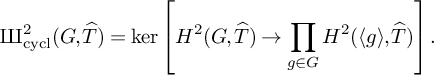
Let $M/k$
be a finite extension with M linearly disjoint from L, and let
$M/k$
be a finite extension with M linearly disjoint from L, and let $L'=LM, K'=KM, k'=kM$
. Then the extension
$L'=LM, K'=KM, k'=kM$
. Then the extension $K'/k'$
has degree n and Galois closure
$K'/k'$
has degree n and Galois closure $L'$
, with
$L'$
, with $\mathrm {Gal}(L'/k') = G$
. Moreover, by a construction of Frölich [Reference Fröhlich19], we may choose M in such a way that
$\mathrm {Gal}(L'/k') = G$
. Moreover, by a construction of Frölich [Reference Fröhlich19], we may choose M in such a way that $L'/k'$
is unramified.
$L'/k'$
is unramified.
Using [Reference Bayer-Fluckiger and Parimala2, Proposition 4.1], we have ![]() , where
, where $\widehat {T}$
is regarded as a
$\widehat {T}$
is regarded as a $\mathrm {Gal}(k^{\prime }_s/k')$
-module via the surjection
$\mathrm {Gal}(k^{\prime }_s/k')$
-module via the surjection $\mathrm {Gal}(k^{\prime }_s/k') \rightarrow G$
. In turn, this is isomorphic to
$\mathrm {Gal}(k^{\prime }_s/k') \rightarrow G$
. In turn, this is isomorphic to ![]() by Poitou–Tate duality [Reference Bayer-Fluckiger and Parimala2, Corollary 4.5]. To summarise, we have isomorphisms
by Poitou–Tate duality [Reference Bayer-Fluckiger and Parimala2, Corollary 4.5]. To summarise, we have isomorphisms
and so it suffices to show that ![]() . However,
. However, ![]() is isomorhpic to the knot group
is isomorhpic to the knot group $\kappa (K'/k') = \frac {k^{\prime \times }\cap N_{K'/k'}(\mathbb {A}_{K'}^{\times })}{N_{K'/k'}(k^{\prime \times })}$
. Due to the assumption
$\kappa (K'/k') = \frac {k^{\prime \times }\cap N_{K'/k'}(\mathbb {A}_{K'}^{\times })}{N_{K'/k'}(k^{\prime \times })}$
. Due to the assumption $\mathrm {Gal}(L'/k') = G = S_n$
, we may apply the result of Kunyavskiı̆ and Voskresenskiı̆ [32] to deduce that the Hasse norm principle holds for the extension
$\mathrm {Gal}(L'/k') = G = S_n$
, we may apply the result of Kunyavskiı̆ and Voskresenskiı̆ [32] to deduce that the Hasse norm principle holds for the extension $K'/k'$
, and hence
$K'/k'$
, and hence $\kappa (K'/k')=0$
.
$\kappa (K'/k')=0$
.
A.3 Proof of Theorem A.1
Before commencing with the proof, we require one more fact about the smooth projective model X from the statement of Theorem A.1.
Lemma A.3. In the notation of Theorem A.1, the base change $X_K = X \times _k K$
is a K-rational variety.
$X_K = X \times _k K$
is a K-rational variety.
Proof. Since X is a smooth projective model of Y, it suffices to show that $Y_K$
is K-rational. Let
$Y_K$
is K-rational. Let $K = k[x]/(p(x))$
, where
$K = k[x]/(p(x))$
, where $p(x)$
is an irreducible polynomial over k. Let a denote the class of x. Over K, the polynomial
$p(x)$
is an irreducible polynomial over k. Let a denote the class of x. Over K, the polynomial $p(x)$
factorises as
$p(x)$
factorises as $p(x) =\prod _{i=0}^r q_i(x)$
, where
$p(x) =\prod _{i=0}^r q_i(x)$
, where $q_0(x), \ldots , q_r(x) \in K[x]$
are distinct and irreducible, and
$q_0(x), \ldots , q_r(x) \in K[x]$
are distinct and irreducible, and $q_0(x) = x-a$
. Let
$q_0(x) = x-a$
. Let $K_i = K[x]/(q_i(x))$
. We shall construct a birational map of the form
$K_i = K[x]/(q_i(x))$
. We shall construct a birational map of the form
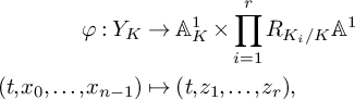 $$ \begin{align} \begin{aligned} \varphi: Y_K &\rightarrow \mathbb{A}^1_K \times \prod_{i=1}^r R_{K_i/K}\mathbb{A}^1\\ (t,x_0, \ldots, x_{n-1}) &\mapsto (t,z_1, \ldots, z_r), \end{aligned} \end{align} $$
where $R_{K_i/K}$
denotes the Weil restriction. Since
$R_{K_i/K}$
denotes the Weil restriction. Since $R_{K_i/K}\mathbb {A}^1 \cong \mathbb {A}^{\deg q_i}_K$
, the right-hand side of (A.3) is isomorphic to
$R_{K_i/K}\mathbb {A}^1 \cong \mathbb {A}^{\deg q_i}_K$
, the right-hand side of (A.3) is isomorphic to $\mathbb {A}^n_K$
, which is a Zariski open subset of
$\mathbb {A}^n_K$
, which is a Zariski open subset of $\mathbb {P}^n_K$
. Therefore,
$\mathbb {P}^n_K$
. Therefore, $\varphi $
induces a birational map
$\varphi $
induces a birational map $Y_K \dashrightarrow \mathbb {P}^n_K$
, as desired.
$Y_K \dashrightarrow \mathbb {P}^n_K$
, as desired.
Let $\overline {k}$
denote an algebraic closure of k. We denote by
$\overline {k}$
denote an algebraic closure of k. We denote by $\operatorname {Emb}_k(K, \overline {k})$
the embeddings
$\operatorname {Emb}_k(K, \overline {k})$
the embeddings $K\hookrightarrow \overline {k}$
fixing k, or in other words, the conjugates of
$K\hookrightarrow \overline {k}$
fixing k, or in other words, the conjugates of $K/k$
in
$K/k$
in $\overline {k}$
. Over
$\overline {k}$
. Over $\overline {k}$
, the polynomials
$\overline {k}$
, the polynomials $p(x), q_0(x), \ldots , q_r(x)$
split as
$p(x), q_0(x), \ldots , q_r(x)$
split as
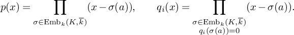 $$ \begin{align} p(x) = \prod_{\sigma \in \operatorname{Emb}_k(K,\overline{k})}(x-\sigma(a)), \qquad q_i(x) = \prod_{\substack{\sigma \in \operatorname{Emb}_k(K,\overline{k})\\ q_i(\sigma(a))=0}}(x-\sigma(a)). \end{align} $$
For each i, we fix an isomorphism $K_i \cong K(\sigma _i(a))$
for some
$K_i \cong K(\sigma _i(a))$
for some $\sigma _i \in \operatorname {Emb}_k(K,\overline {k})$
satisfying
$\sigma _i \in \operatorname {Emb}_k(K,\overline {k})$
satisfying $q_i(\sigma _i(a))=0$
, and view
$q_i(\sigma _i(a))=0$
, and view $\sigma _i(a)$
as the class of x in
$\sigma _i(a)$
as the class of x in $K_i/K$
. (The particular choice of representative
$K_i/K$
. (The particular choice of representative $\sigma _i$
does not matter.) Since
$\sigma _i$
does not matter.) Since $q_i(x)$
is the minimum polynomial of
$q_i(x)$
is the minimum polynomial of $\sigma _i(a)$
over K, it splits over
$\sigma _i(a)$
over K, it splits over $\overline {k}$
as the product of the conjugates of
$\overline {k}$
as the product of the conjugates of $\sigma _i(a)$
, and so
$\sigma _i(a)$
, and so
 $$ \begin{align*}q_i(x) = \prod_{\sigma' \in \operatorname{Emb}_K(K_i, \overline{k})}(x - \sigma'\sigma_i(a)).\end{align*} $$
For $i\in \{0,\ldots , r\}$
, we define
$i\in \{0,\ldots , r\}$
, we define $z_i \in R_{K_i/K}\mathbb {A}^1$
as
$z_i \in R_{K_i/K}\mathbb {A}^1$
as
 $$ \begin{align} z_i = x_0+\sigma_i(a)x_1 + \cdots + \sigma_i(a)^{n-1}x_{n-1}. \end{align} $$
The polynomial $\sum _{j=0}^{\deg q_i -1}z_i^{(j)}x^j$
representing
$\sum _{j=0}^{\deg q_i -1}z_i^{(j)}x^j$
representing $z_i$
is the reduction of
$z_i$
is the reduction of $x_0 + x_1x + \cdots + x_{n-1}x^{n-1}$
modulo
$x_0 + x_1x + \cdots + x_{n-1}x^{n-1}$
modulo $q_i$
. Consequently, by the Chinese remainder theorem,
$q_i$
. Consequently, by the Chinese remainder theorem, $z_0, \ldots , z_r \in \prod _{i=0}^r R_{K_i/K}\mathbb {A}^1$
uniquely determine
$z_0, \ldots , z_r \in \prod _{i=0}^r R_{K_i/K}\mathbb {A}^1$
uniquely determine $x_0, \ldots , x_{n-1} \in \mathbb {A}^1_K$
.
$x_0, \ldots , x_{n-1} \in \mathbb {A}^1_K$
.
For any number field extension $E/M$
, and any
$E/M$
, and any $y \in E$
, we have
$y \in E$
, we have
 $$ \begin{align*}N_{E/M}(y) = \prod_{\sigma \in \operatorname{Emb}_M(E,\overline{M})} \sigma (y).\end{align*} $$
Therefore,
 $$ \begin{align*} N_{K/k}(y) = \prod_{\sigma \in \operatorname{Emb}_k(K,\overline{k})}\sigma(y) = \prod_{i=0}^r \prod_{\sigma' \in \operatorname{Emb}_{K}(K_i, \overline{k})}\sigma'\sigma_i(y) = \prod_{i=0}^r N_{K_i/K}(\sigma_i(y)), \end{align*} $$
and so
 $$ \begin{align} \mathbf{N}(x_0, \ldots, x_{n-1}) = \prod_{i=0}^r N_{K_i/K}(z_i). \end{align} $$
We deduce that the equations (A.5) define an isomorphism from $Y_K$
to the variety
$Y_K$
to the variety $V\subseteq \mathbb {A}^1_K \times \prod _{i=0}^rR_{K_i/K}\mathbb {A}^1$
given by
$V\subseteq \mathbb {A}^1_K \times \prod _{i=0}^rR_{K_i/K}\mathbb {A}^1$
given by $z_0\prod _{i=1}^r N_{K_i/K}(z_i) = f(t)\neq 0$
. For
$z_0\prod _{i=1}^r N_{K_i/K}(z_i) = f(t)\neq 0$
. For $t,z_1, \ldots , z_r$
satisfying the Zariski open condition
$t,z_1, \ldots , z_r$
satisfying the Zariski open condition $\prod _{i=1}^r N_{K_i/K}(z_i) \neq 0$
, we have
$\prod _{i=1}^r N_{K_i/K}(z_i) \neq 0$
, we have $z_0 = f(t)/\prod _{i=1}^n N_{K_i/K}(z_i)$
. Therefore, the projection of V onto
$z_0 = f(t)/\prod _{i=1}^n N_{K_i/K}(z_i)$
. Therefore, the projection of V onto $\mathbb {A}^1_K \times \prod _{i=1}^r R_{K_i/K}\mathbb {A}^1$
is birational. We conclude that the map
$\mathbb {A}^1_K \times \prod _{i=1}^r R_{K_i/K}\mathbb {A}^1$
is birational. We conclude that the map $\varphi $
from (A.3) is birational.
$\varphi $
from (A.3) is birational.
We now commence with the proof of Theorem A.1. Let k be a field of characteristic zero. For a smooth irreducible variety $X/k$
with function field
$X/k$
with function field $\kappa (x)$
, we recall that
$\kappa (x)$
, we recall that $\operatorname {\mathrm {Br}}(X)$
consists of all elements of
$\operatorname {\mathrm {Br}}(X)$
consists of all elements of $\operatorname {\mathrm {Br}}(\kappa (X))$
which are unramified everywhere on X. Constant classes are unramified, and so we have
$\operatorname {\mathrm {Br}}(\kappa (X))$
which are unramified everywhere on X. Constant classes are unramified, and so we have $\operatorname {\mathrm {Br}}(k) \subseteq \operatorname {\mathrm {Br}}(X) \subseteq \operatorname {\mathrm {Br}}(\kappa (X))$
. By the purity theorem [Reference Colliot-Thélène and Skorobogatov11, Theorem 3.7.1], the ramification locus of
$\operatorname {\mathrm {Br}}(k) \subseteq \operatorname {\mathrm {Br}}(X) \subseteq \operatorname {\mathrm {Br}}(\kappa (X))$
. By the purity theorem [Reference Colliot-Thélène and Skorobogatov11, Theorem 3.7.1], the ramification locus of $\mathcal {A}\in \operatorname {\mathrm {Br}}(\kappa (X))$
is pure of codimension one. Consequently, to check
$\mathcal {A}\in \operatorname {\mathrm {Br}}(\kappa (X))$
is pure of codimension one. Consequently, to check $\mathcal {A} \in \operatorname {\mathrm {Br}}(X)$
, it suffices to check it is unramified at all codimension one points of X.
$\mathcal {A} \in \operatorname {\mathrm {Br}}(X)$
, it suffices to check it is unramified at all codimension one points of X.
Let C be a codimension one point. We recall from [Reference Colliot-Thélène and Skorobogatov11, Section 1.4.3] the residue map
 $$ \begin{align*}\partial_C: \operatorname{\mathrm{Br}}(\kappa (X)) \rightarrow H^1(\kappa(C), \mathbb{Q}/\mathbb{Z})\end{align*} $$
is such that $\mathcal {A}$
is unramified at C if and only if
$\mathcal {A}$
is unramified at C if and only if $\partial _C(\mathcal {A})$
is trivial.
$\partial _C(\mathcal {A})$
is trivial.
In our setting, codimension one points of X come in two types:
-
(1) Irreducible components of fibres
$X_c = \pi ^{-1}(c)$
above codimension one points c of
$\mathbb {P}_k^1$
, -
(2) Codimension one points on the generic fibre
$X_{\eta }$
of
$\pi :X\rightarrow \mathbb {P}_k^1$
.


We recall that $\kappa (X) = \kappa (X_\eta )$
. The codimension one points of
$\kappa (X) = \kappa (X_\eta )$
. The codimension one points of $X_{\eta }$
are a subset of the codimension one points of X, and so we have an inclusion
$X_{\eta }$
are a subset of the codimension one points of X, and so we have an inclusion $\operatorname {\mathrm {Br}}(X) \hookrightarrow \operatorname {\mathrm {Br}}(X_{\eta })$
. Since
$\operatorname {\mathrm {Br}}(X) \hookrightarrow \operatorname {\mathrm {Br}}(X_{\eta })$
. Since $X_{\eta }$
is a smooth projective model of
$X_{\eta }$
is a smooth projective model of $\mathbf {N}_{K(t)/k(t)}(x_1, \ldots , x_n) = f(t)$
over
$\mathbf {N}_{K(t)/k(t)}(x_1, \ldots , x_n) = f(t)$
over $k(t)$
, it follows from Theorem A.2, applied to the extension
$k(t)$
, it follows from Theorem A.2, applied to the extension $K(t)/k(t)$
and with
$K(t)/k(t)$
and with $Z=X_{\eta }$
, that
$Z=X_{\eta }$
, that $\operatorname {\mathrm {Br}}(k(t)) \rightarrow \operatorname {\mathrm {Br}}(X_{\eta })$
is surjective. Putting everything together, we obtain a commutative diagram
$\operatorname {\mathrm {Br}}(k(t)) \rightarrow \operatorname {\mathrm {Br}}(X_{\eta })$
is surjective. Putting everything together, we obtain a commutative diagram
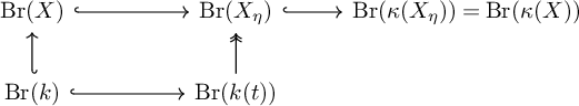
Let $\alpha \in \operatorname {\mathrm {Br}}(X)$
. By the above diagram, we can find
$\alpha \in \operatorname {\mathrm {Br}}(X)$
. By the above diagram, we can find $\beta \in \operatorname {\mathrm {Br}}(k(t))$
whose image in
$\beta \in \operatorname {\mathrm {Br}}(k(t))$
whose image in $\operatorname {\mathrm {Br}}(X_{\eta })$
is equal to the image of
$\operatorname {\mathrm {Br}}(X_{\eta })$
is equal to the image of $\alpha $
in
$\alpha $
in $\operatorname {\mathrm {Br}}(X_{\eta })$
. We want to show that
$\operatorname {\mathrm {Br}}(X_{\eta })$
. We want to show that $\beta $
is the image of an element of
$\beta $
is the image of an element of $\operatorname {\mathrm {Br}}(k)$
because then it follows from commutativity of the diagram that
$\operatorname {\mathrm {Br}}(k)$
because then it follows from commutativity of the diagram that $\alpha $
is the image of an element of
$\alpha $
is the image of an element of $\operatorname {\mathrm {Br}}(k)$
.
$\operatorname {\mathrm {Br}}(k)$
.
For any $n\geqslant 1$
and any field k, we have
$n\geqslant 1$
and any field k, we have $\operatorname {\mathrm {Br}}(\mathbb {P}_k^n) = \operatorname {\mathrm {Br}}(k)$
[Reference Colliot-Thélène and Skorobogatov11, Theorem 6.1.3]. In particular, we have
$\operatorname {\mathrm {Br}}(\mathbb {P}_k^n) = \operatorname {\mathrm {Br}}(k)$
[Reference Colliot-Thélène and Skorobogatov11, Theorem 6.1.3]. In particular, we have $\operatorname {\mathrm {Br}}(k) = \operatorname {\mathrm {Br}}(\mathbb {P}_k^1)$
. Also,
$\operatorname {\mathrm {Br}}(k) = \operatorname {\mathrm {Br}}(\mathbb {P}_k^1)$
. Also, $k(t) = \kappa (\mathbb {P}_k^1)$
, so
$k(t) = \kappa (\mathbb {P}_k^1)$
, so $\operatorname {\mathrm {Br}}(k(t)) = \operatorname {\mathrm {Br}}(\kappa (\mathbb {P}_k^1))$
. Therefore, as discussed above, to prove that
$\operatorname {\mathrm {Br}}(k(t)) = \operatorname {\mathrm {Br}}(\kappa (\mathbb {P}_k^1))$
. Therefore, as discussed above, to prove that $\beta $
is in the image of
$\beta $
is in the image of $\operatorname {\mathrm {Br}}(k)$
, it suffices to show
$\operatorname {\mathrm {Br}}(k)$
, it suffices to show $\beta $
is unramified at every codimension one point of
$\beta $
is unramified at every codimension one point of $\mathbb {P}^1_k$
. This is formalised by the Faddeev exact sequence [Reference Colliot-Thélène and Skorobogatov11, Theorem 1.5.2], which is the exact sequence
$\mathbb {P}^1_k$
. This is formalised by the Faddeev exact sequence [Reference Colliot-Thélène and Skorobogatov11, Theorem 1.5.2], which is the exact sequence
 $$ \begin{align} 0 \rightarrow \operatorname{\mathrm{Br}}(k) \hookrightarrow \operatorname{\mathrm{Br}}(k(t)) \rightarrow \bigoplus_{Q\in (\mathbb{P}^1_k)^{(1)}} H^1(k_Q , \mathbb{Q}/\mathbb{Z}) \twoheadrightarrow H^1(k, \mathbb{Q}/\mathbb{Z}) \rightarrow 0, \end{align} $$
where $(\mathbb {P}^1_k)^{(1)}$
denotes the codimension one points of
$(\mathbb {P}^1_k)^{(1)}$
denotes the codimension one points of $\mathbb {P}_k^1$
and the third map is the direct sum of the residue maps
$\mathbb {P}_k^1$
and the third map is the direct sum of the residue maps $\partial _Q$
. In other words, to show that
$\partial _Q$
. In other words, to show that $\beta \in \operatorname {\mathrm {Br}}(k(t))$
is actually in
$\beta \in \operatorname {\mathrm {Br}}(k(t))$
is actually in $\operatorname {\mathrm {Br}}(k)$
, it suffices to show that
$\operatorname {\mathrm {Br}}(k)$
, it suffices to show that $\partial _Q(\beta ) = 0$
for all
$\partial _Q(\beta ) = 0$
for all $Q \in (\mathbb {P}_k^1)^{(1)}$
. We have
$Q \in (\mathbb {P}_k^1)^{(1)}$
. We have $\partial _Q(\beta ) = 0$
unless Q is an irreducible factor of
$\partial _Q(\beta ) = 0$
unless Q is an irreducible factor of $f(t)$
by [Reference Colliot-Thélène and Skorobogatov11, Proposition 11.1.5], so we suppose from now on that Q is an irreducible factor of
$f(t)$
by [Reference Colliot-Thélène and Skorobogatov11, Proposition 11.1.5], so we suppose from now on that Q is an irreducible factor of $f(t)$
.
$f(t)$
.
By Lemma A.3, the base change $X_K = X \times _{k} K$
is birational to
$X_K = X \times _{k} K$
is birational to $\mathbb {P}_K^n$
. Since the Brauer group is a birational invariant on smooth projective varieties [Reference Colliot-Thélène and Skorobogatov11, Corollary 6.2.11], it follows that
$\mathbb {P}_K^n$
. Since the Brauer group is a birational invariant on smooth projective varieties [Reference Colliot-Thélène and Skorobogatov11, Corollary 6.2.11], it follows that $\operatorname {\mathrm {Br}}(X_K) = \operatorname {\mathrm {Br}}(\mathbb {P}^n_K) = \operatorname {\mathrm {Br}}(K)$
. Therefore, we obtain the following commutative diagram:
$\operatorname {\mathrm {Br}}(X_K) = \operatorname {\mathrm {Br}}(\mathbb {P}^n_K) = \operatorname {\mathrm {Br}}(K)$
. Therefore, we obtain the following commutative diagram:
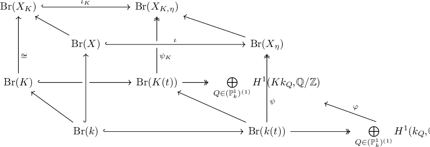
The map $\varphi $
is a direct sum over the restriction maps
$\varphi $
is a direct sum over the restriction maps $\varphi _Q:H^1(k_Q, \mathbb {Q}/\mathbb {Z})\rightarrow H^1(Kk_Q, \mathbb {Q}/\mathbb {Z})$
for each
$\varphi _Q:H^1(k_Q, \mathbb {Q}/\mathbb {Z})\rightarrow H^1(Kk_Q, \mathbb {Q}/\mathbb {Z})$
for each $Q \in (\mathbb {P}^1_k)^{(1)}$
.
$Q \in (\mathbb {P}^1_k)^{(1)}$
.
Lemma A.4. We have $\partial _Q(\beta ) \in \ker \varphi _Q$
, where
$\partial _Q(\beta ) \in \ker \varphi _Q$
, where $\varphi _Q$
is as defined above.
$\varphi _Q$
is as defined above.
Proof. Let $\beta _K$
denote the image of
$\beta _K$
denote the image of $\beta $
in
$\beta $
in $\operatorname {\mathrm {Br}}(K(t))$
, and
$\operatorname {\mathrm {Br}}(K(t))$
, and $\partial _{K,Q}$
the residue map at Q on
$\partial _{K,Q}$
the residue map at Q on $\operatorname {\mathrm {Br}}(K(t))$
. We want to show that
$\operatorname {\mathrm {Br}}(K(t))$
. We want to show that $\partial _{K,Q}(\beta _K) = 0$
. By exactness of the Faddeev exact sequence over K, for this it suffices to show
$\partial _{K,Q}(\beta _K) = 0$
. By exactness of the Faddeev exact sequence over K, for this it suffices to show $\beta _K$
is in the image
$\beta _K$
is in the image $\operatorname {\mathrm {Br}}(K) \rightarrow \operatorname {\mathrm {Br}}(K(t))$
. We know that
$\operatorname {\mathrm {Br}}(K) \rightarrow \operatorname {\mathrm {Br}}(K(t))$
. We know that $\psi (\beta ) = \iota (\alpha )$
. Applying a base change to K, we see that
$\psi (\beta ) = \iota (\alpha )$
. Applying a base change to K, we see that $\psi _K(\beta _K) = \iota _K(\alpha _K)$
, where
$\psi _K(\beta _K) = \iota _K(\alpha _K)$
, where $\alpha _K, \beta _K$
are the images of
$\alpha _K, \beta _K$
are the images of $\alpha , \beta $
under base change. Since
$\alpha , \beta $
under base change. Since $\operatorname {\mathrm {Br}}(K) \cong \operatorname {\mathrm {Br}}(X_K)$
, we have that
$\operatorname {\mathrm {Br}}(K) \cong \operatorname {\mathrm {Br}}(X_K)$
, we have that $\alpha _K$
is in the image of
$\alpha _K$
is in the image of $\operatorname {\mathrm {Br}}(K) \rightarrow \operatorname {\mathrm {Br}}(X_K)$
, and hence by commutativity of the diagram,
$\operatorname {\mathrm {Br}}(K) \rightarrow \operatorname {\mathrm {Br}}(X_K)$
, and hence by commutativity of the diagram, $\beta _K$
is in the image of
$\beta _K$
is in the image of $\operatorname {\mathrm {Br}}(K) \rightarrow \operatorname {\mathrm {Br}}(K(t))$
, as required.
$\operatorname {\mathrm {Br}}(K) \rightarrow \operatorname {\mathrm {Br}}(K(t))$
, as required.
Let M be a number field, and let $G_M = \mathrm {Gal}(\overline {M}/M)$
. For a finite Galois extension
$G_M = \mathrm {Gal}(\overline {M}/M)$
. For a finite Galois extension $M'/M$
, we consider
$M'/M$
, we consider $\mathrm {Gal}(M'/M)$
as a topological space with the discrete topology. We can then put the profinite topology on
$\mathrm {Gal}(M'/M)$
as a topological space with the discrete topology. We can then put the profinite topology on $G_M$
, which is defined as the inverse limit
$G_M$
, which is defined as the inverse limit
 $$ \begin{align*}G_M = \varprojlim_{M'/M \textrm{ Galois}} \mathrm{Gal}(M'/M).\end{align*} $$
We recall that $H^1(M,\mathbb {Q}/\mathbb {Z}) = \operatorname {Hom}_{\textrm {cont}}(G_M, \mathbb {Q}/\mathbb {Z})$
, the continuous group homomorphisms
$H^1(M,\mathbb {Q}/\mathbb {Z}) = \operatorname {Hom}_{\textrm {cont}}(G_M, \mathbb {Q}/\mathbb {Z})$
, the continuous group homomorphisms $G_M \rightarrow \mathbb {Q}/\mathbb {Z}$
[Reference Colliot-Thélène and Skorobogatov11, pp.16]. Suppose that
$G_M \rightarrow \mathbb {Q}/\mathbb {Z}$
[Reference Colliot-Thélène and Skorobogatov11, pp.16]. Suppose that $\theta \in \operatorname {Hom}_{\textrm {cont}}(G_M, \mathbb {Q}/\mathbb {Z})$
. Then
$\theta \in \operatorname {Hom}_{\textrm {cont}}(G_M, \mathbb {Q}/\mathbb {Z})$
. Then $\ker \theta $
is an open subgroup of
$\ker \theta $
is an open subgroup of $G_M$
. Since
$G_M$
. Since $G_M$
is a profinite group, this implies that
$G_M$
is a profinite group, this implies that $\ker \theta $
has finite index in
$\ker \theta $
has finite index in $G_M$
. By the fundamental theorem of Galois theory,
$G_M$
. By the fundamental theorem of Galois theory, $\operatorname {im}\theta \cong G_M/\ker \theta \cong \mathrm { Gal}(M'/M)$
, for some finite Galois extension
$\operatorname {im}\theta \cong G_M/\ker \theta \cong \mathrm { Gal}(M'/M)$
, for some finite Galois extension $M'/M$
. Moreover,
$M'/M$
. Moreover, $\operatorname {im}\theta $
is a finite subgroup of
$\operatorname {im}\theta $
is a finite subgroup of $\mathbb {Q}/\mathbb {Z}$
. All finite subgroups of
$\mathbb {Q}/\mathbb {Z}$
. All finite subgroups of $\mathbb {Q}/\mathbb {Z}$
are cyclic groups of the form
$\mathbb {Q}/\mathbb {Z}$
are cyclic groups of the form $\frac {1}{n}\mathbb {Z}/\mathbb {Z}$
for some positive integer n. Consequently,
$\frac {1}{n}\mathbb {Z}/\mathbb {Z}$
for some positive integer n. Consequently, $\ker \theta = \mathrm {Gal}(M'/M)$
for a cyclic extension
$\ker \theta = \mathrm {Gal}(M'/M)$
for a cyclic extension $M'/M$
. To summarise, we have the identification
$M'/M$
. To summarise, we have the identification
 $$ \begin{align*}H^1(M, \mathbb{Q}/\mathbb{Z}) = \{M'/M \textrm{ cyclic, with a given map }\gamma:\mathrm{Gal}(M'/M) \hookrightarrow \mathbb{Q}/\mathbb{Z}\}.\end{align*} $$
We now describe $\varphi _Q: H^1(k_Q, \mathbb {Q}/\mathbb {Z}) \rightarrow H^1(Kk_Q, \mathbb {Q}/\mathbb {Z})$
explicitly. Using the above identification, we view an element
$\varphi _Q: H^1(k_Q, \mathbb {Q}/\mathbb {Z}) \rightarrow H^1(Kk_Q, \mathbb {Q}/\mathbb {Z})$
explicitly. Using the above identification, we view an element $\theta \in H^1(k_Q, \mathbb {Q}/\mathbb {Z})$
as a pair
$\theta \in H^1(k_Q, \mathbb {Q}/\mathbb {Z})$
as a pair $(M'/k_Q, \gamma )$
. The map
$(M'/k_Q, \gamma )$
. The map $\varphi _Q$
is given by taking the compositum with K. More precisely, it sends the above pair to
$\varphi _Q$
is given by taking the compositum with K. More precisely, it sends the above pair to $(KM'/Kk_Q, \gamma )$
, where now
$(KM'/Kk_Q, \gamma )$
, where now $\gamma $
is viewed as a map
$\gamma $
is viewed as a map $\mathrm {Gal}(KM'/KK_Q) \hookrightarrow \mathbb {Q}/\mathbb {Z}$
via the natural identification of
$\mathrm {Gal}(KM'/KK_Q) \hookrightarrow \mathbb {Q}/\mathbb {Z}$
via the natural identification of $\mathrm {Gal}(KM'/Kk_Q)$
as a subgroup of
$\mathrm {Gal}(KM'/Kk_Q)$
as a subgroup of $\mathrm {Gal}(M'/k_Q)$
. Therefore,
$\mathrm {Gal}(M'/k_Q)$
. Therefore, $(M'/k_Q, \gamma ) \in \ker \varphi _Q$
if and only if
$(M'/k_Q, \gamma ) \in \ker \varphi _Q$
if and only if $M'/k_Q$
is a cyclic subextension of
$M'/k_Q$
is a cyclic subextension of $Kk_Q/k_Q$
.
$Kk_Q/k_Q$
.
Due to the assumption that $k_Q$
and L are linearly disjoint over k, we have
$k_Q$
and L are linearly disjoint over k, we have $\mathrm {Gal}(Kk_Q/k_Q) \cong \mathrm {Gal}(K/k) \cong S_n$
. We now complete the proof of Theorem A.1 with the following elementary group theory fact.
$\mathrm {Gal}(Kk_Q/k_Q) \cong \mathrm {Gal}(K/k) \cong S_n$
. We now complete the proof of Theorem A.1 with the following elementary group theory fact.
Lemma A.5. Suppose that $K/k$
is a finite extension of degree
$K/k$
is a finite extension of degree $n\geqslant 3$
, and the Galois group of the Galois closure
$n\geqslant 3$
, and the Galois group of the Galois closure $\mathrm {Gal}(L/k)$
is isomorphic to
$\mathrm {Gal}(L/k)$
is isomorphic to $S_n$
. Then there are no nontrivial cyclic extensions
$S_n$
. Then there are no nontrivial cyclic extensions $M/k$
with
$M/k$
with $M\subseteq K$
.
$M\subseteq K$
.
Proof. By the fundamental theorem of Galois theory, if $M/k$
is a subextension of
$M/k$
is a subextension of $K/k$
, then
$K/k$
, then $\mathrm {Gal}(L/K) \leqslant \mathrm {Gal}(L/M) \leqslant \mathrm { Gal}(L/k) = S_n$
. However,
$\mathrm {Gal}(L/K) \leqslant \mathrm {Gal}(L/M) \leqslant \mathrm { Gal}(L/k) = S_n$
. However, $\mathrm {Gal}(L/K) \cong S_{n-1}$
. (More explicitly, if
$\mathrm {Gal}(L/K) \cong S_{n-1}$
. (More explicitly, if $K=k(\alpha _1)$
and
$K=k(\alpha _1)$
and $\alpha _1, \ldots , \alpha _n$
are the roots of the minimum polynomial of
$\alpha _1, \ldots , \alpha _n$
are the roots of the minimum polynomial of $\alpha _1$
over k, then
$\alpha _1$
over k, then $\mathrm {Gal}(L/K)$
consists of all permutations of
$\mathrm {Gal}(L/K)$
consists of all permutations of $\{\alpha _1, \ldots , \alpha _n\}$
which fix
$\{\alpha _1, \ldots , \alpha _n\}$
which fix $\alpha _1$
.) However,
$\alpha _1$
.) However, $S_{n-1}$
is a maximal subgroup of
$S_{n-1}$
is a maximal subgroup of $S_n$
, and so
$S_n$
, and so $M=k$
or
$M=k$
or $M=K$
. Since
$M=K$
. Since $n\geqslant 3$
, the extension
$n\geqslant 3$
, the extension $K/k$
is not cyclic. Therefore,
$K/k$
is not cyclic. Therefore, $M=k$
.
$M=k$
.
In conclusion, the map $\varphi _Q$
is injective by Lemma A.5, and
$\varphi _Q$
is injective by Lemma A.5, and $\partial _Q(\beta ) \in \ker \varphi _Q$
by Lemma A.4, and hence
$\partial _Q(\beta ) \in \ker \varphi _Q$
by Lemma A.4, and hence $\partial _Q(\beta )=0$
. This means that all the residue maps of
$\partial _Q(\beta )=0$
. This means that all the residue maps of $\beta $
are trivial, so
$\beta $
are trivial, so $\beta $
is in the image of
$\beta $
is in the image of $\operatorname {\mathrm {Br}}(k) \rightarrow \operatorname {\mathrm {Br}}(k(t))$
. Hence,
$\operatorname {\mathrm {Br}}(k) \rightarrow \operatorname {\mathrm {Br}}(k(t))$
. Hence, $\alpha $
is in the image of
$\alpha $
is in the image of $\operatorname {\mathrm {Br}}(k) \rightarrow \operatorname {\mathrm {Br}}(X)$
, and so
$\operatorname {\mathrm {Br}}(k) \rightarrow \operatorname {\mathrm {Br}}(X)$
, and so $\operatorname {\mathrm {Br}}(X) = \operatorname {\mathrm {Br}}(k)$
. This completes the proof of Theorem A.1.
$\operatorname {\mathrm {Br}}(X) = \operatorname {\mathrm {Br}}(k)$
. This completes the proof of Theorem A.1.
Acknowledgements
The author is grateful to Jean-Louis Colliot-Thélène for providing the statements and proofs in Appendix A, and to Julian Lyczak and Alexei Skorobogatov for helpful discussions on Brauer groups. The author would like to thank Olivier Wittenberg for many useful comments on the Harpaz–Wittenberg conjecture, including suggesting the statement and proof of Proposition 6.6, and to Florian Wilsch for helpful discussions and feedback on an earlier version of Section 6.1. The author would like to thank Tim Browning for valuable feedback and guidance during the development of this work. Finally, the author is grateful to the anonymous referee for many useful comments on an earlier version of this paper. The author is supported by the University of Bristol and the Heilbronn Institute for Mathematical Research.
Competing interests
The authors have no competing interest to declare.
Data availability
No new data were created or analysed in this study. Data sharing is not applicable to this article.

 Open access