


1. Transportation on the sphere
Optimal transportation involves moving unit mass from one probability distribution to another, at minimal cost, where the cost is measured by Wasserstein's distance.
Definition Let $(M,\,d)$ be a compact metric space and let $\mu$
 and $\nu$
 be probability measures on $M$
 . Then for $1\leq p<\infty$
 , Wasserstein's distance from $\mu$
 to $\nu$
 is $W_p(\nu,\, \mu )$
 , where

where the probability measure $\pi$ has marginals $\nu$
 and $\mu$
 (see [Reference Dudley8, Reference Villani14]).
Transportation inequalities are results that bound the transportation cost $W_p(\nu,\, \mu )^p$ in terms of $\mu$
 , $\nu$
 and geometrical quantities of $(M,\,d)$
 . Typically, one chooses $\mu$
 to satisfy special conditions, and then one imposes minimal hypotheses on $\nu$
 . In this section, we consider the case where $(M,\,d)$
 is the unit sphere ${\bf S}^2$
 in ${\bf R}^3$
 , and obtain transportation inequalities by vector calculus. In section two, we extend these methods to a connected, compact and $C^\infty$
 smooth Riemannian manifold $(M,\,d)$
 .
.
On ${\bf S}^2$ , let $\theta \in [0,\, 2\pi )$
 be the longitude and $\phi \in [0,\, \pi ]$
 the colatitude, so the area measure is ${\rm d}x=\sin \phi \, d\phi d\theta$
 . Let $ABC$
 be a spherical triangle where $A$
 is the North Pole; then by [Reference Kimura and Okamoto10] the Green's function $G(B,\,C)=-(4\pi )^{-1}\log (1-\cos d(B,\,C))$
 may be expressed in terms of longitude and co latitude of $B$
 and $C$
 via the spherical cosine formula. A related cost function is listed in [Reference Villani14], p 972. Given probability measures $\mu$
 and $\nu$
 on ${\bf S}^2$
 , we can form

with gradient in the $x$ variable

Proposition 1.1 Let $\mu$ and $\nu$
 be nonatomic probability measures on ${\bf S}^2$
 . Then

Proof. The Green's function is chosen so that $\nabla \cdot \nabla G(B,\,C)=\delta _B(C)-1/(4\pi )$ in the sense of distributions. Given non-atomic probability measures $\mu$
 and $\nu$
 on ${\bf S}^2$
 , their difference $\mu -\nu$
 is orthogonal to the constants on ${\bf S}^2,$
 so for a $1$
 -Lipschitz function $\varphi : {\bf S}^2\rightarrow {\bf R}$
 , we have

so by Kantorovich's duality theorem [Reference Dudley8], the Wasserstein transportation distance is bounded by

Definition Suppose that $\mu$ is a probability measure and $\nu$
 is a probability measure that is absolutely continuous with respect to $\mu$
 , so $d\nu =vd\mu$
 for some probability density function $v\in L^1(\mu )$
 . Then the relative entropy of $\nu$
 with respect to $\mu$
 is
is

where $0\leq {\hbox {Ent}}(\nu \mid \mu ) \leq \infty$ by Jensen's inequality.
At $x\in {\bf S}^2$ , we have tangent space $T_s{\bf S}^2=\{ y\in {\bf R}^3: x\cdot y=0\}$
 . For $y\in T_x{\bf S}^2$
 with $\Vert y\Vert =1$
 , we consider $\exp _x(ty)=x\cos t+y\sin t$
 so that $\exp _x(0)=x$
 , $\Vert \exp _x(ty)\Vert =1$
 and $(d/{\rm d}t)_{t=0}\exp _x(ty)=y$
 ; hence $\exp _x:T_x{\bf S}^2\rightarrow {\bf S}^2$
 gives the exponential map. We let $J_{\exp _x}$
 be the Jacobian determinant of this map.
Suppose that $\mu ({\rm d}x)=e^{-U (x)}{\rm d}x$ is a probability measure and $\nu$
 is a probability measure that is absolutely continuous with respect to $\mu$
 , so $d\nu =vd\mu$
 . We say that a Borel function $\Psi :{\bf S}^2\rightarrow {\bf S}^2$
 induces $\nu$
 from $\mu$
 if $\int f(y)\nu ({\rm d}y)=\int f(\Psi (x))\mu ({\rm d}x )$
 for all $f\in C({\bf S}^2; {\bf R})$
 . McCann [Reference McCann12] showed that there exists $\Psi$
 that gives the optimal transport strategy for the $W_2$
 metric; further, there exists a Lipschitz function $\psi : {\bf S}^2\rightarrow {\bf R}$
 such that $\Psi (x)=\exp _x(\nabla \psi (x))$
 ; so that

Talagrand developed $T_p$ inequalities in which $W_p(\nu,\, \mu )^p$
 is bounded in terms of ${\hbox {Ent}}(\nu \mid \mu )$
 , as in [Reference Villani14], p 569. In [Reference Cordero-Erausquin5] and [Reference Cordero-Erausquin, McCann and Schmuckensläger6], the authors obtain some functional inequalities that are related to $T_p$
 inequalities. Here we offer an approach that is more direct, and uses only basic differential geometry to augment McCann's fundamental result. The key point is an explicit formula for the relative entropy in terms of the optimal transport maps.
Lemma 1.2 Suppose that $\nu$ has finite relative entropy with respect to $\mu,$
 and let

let $\Psi _t(x)=\exp _x(t\nabla \psi (x))$ for $t\in [0,\,1]$
 . Then the relative entropy satisfies

where $A$ is positive definite, $H$
 is symmetric and $A+H$
 is also positive definite, and

If $\psi \in C^2,$ then equality holds in (1.8).
Proof. To express the relative entropy in terms of the transportation map, we adapt an argument from [Reference Blower1]. We have ${\hbox {Ent}}(\nu \mid \mu )=\int _{{\bf S}^2} \log v(\Psi (x))\mu ({\rm d}x)$ , where the integrand is

where the final term arises from the Jacobian of the change of variable $y=\Psi (x)$ , where $\Psi =\Psi _1$
 and $\Psi _t(x)=\exp _x(t\nabla \psi (x))$
 . We compute this Jacobian by the chain rule for derivatives with respect to $x$
 . Specifically by [Reference Cordero-Erausquin, McCann and Schmuckensläger6] p 622, we have ${\hbox {Hess}}(\psi (x)+d(x,\,y)^2/2)\geq 0$
 and
and

where $J_{\exp _x}$ is the Jacobian of $\exp _x:T_x{\bf S}^2\rightarrow {\bf S}^2$
 and ${\hbox {Hess}}=D_x^2$
 is the Hessian, where the expression is evaluated at $y=\exp _x(\nabla \psi (x))$
 . For $x\in {\bf S}^2$
 and $\tau \in {\bf R}^3$
 such that $x\cdot \tau =0$
 , we have $\tau \in T_x{\bf S}^2$
 and
and

see [Reference Cordero-Erausquin5]. By a vector calculus computation, which we replicate from [Reference Cordero-Erausquin5], one finds

With $\psi :{\bf S}^2\rightarrow {\bf R}$ we have $\nabla \psi (x)\perp x$
 , so $0=x\cdot \nabla \psi (x),$
 hence $0=\nabla \psi (x)+{\hbox {Hess}}(\psi (x)) x$
 . We write $\theta =\Vert \nabla \psi (x)\Vert$
 for the angle between $x$
 and $\Psi (x)$
 so
so

let $v=x\times \theta ^{-1}\nabla \psi (x)$ where $\times$
 denotes the usual vector product; then $\{ x,\, \theta ^{-1}\nabla \psi (x),\, v\}$
 gives an orthonormal basis of ${\bf R}^3$
 . Hence

and we obtain (1.13) from the final factor. Then by spherical trigonometry, we have

so we have $\langle \nabla _x \cos d(x,\,y),\, \tau \rangle =\langle y,\, \tau \rangle$ and $\langle {\hbox {Hess}}_x\cos d(x,\,y)\tau,\, \tau \rangle =-(\cos d(x,\,y)) \Vert \tau \Vert ^2$
 ; so
; so

hence $A$ is positive definite and is a rank-one perturbation of a multiple of the identity matrix. Note that the formulas degenerate on the cut locus $d(x,\,y)=\pi ;$
 consider the international date line opposite the Greenwich meridian.
We have

in which

and we can combine the first two terms in (1.16) by the divergence theorem so
Hence from (1.11) we have

in which the Alexandrov Hessian [Reference Cordero-Erausquin, McCann and Schmuckensläger6], [Reference Villani14] p 363 satisfies

where $\Delta _D\psi$ is the distributional derivative of the Lipschitz function $\psi$
 ; so we recognize (1.8).
We have an orthonormal basis

for ${\bf R}^3$ in which the final two vectors give an orthonormal basis for $T_x{\bf S}^2$
 . Then

and

hence $A$ and $H$
 have the form

with respect to the stated basis of $T_x{\bf S}^2$ .
.
The function $f(x)=x-1-\log x$ for $x>0$
 is convex and takes its minimum value at $f(1)=0$
 . Let $T$
 be a self-adjoint matrix with eigenvalues $\lambda _1\geq \dots \geq \lambda _n$
 where $\lambda _n>-1$
 ; then the Carleman determinant of $I+T$
 is $\det _2(I+T)=\prod _{j=1}^n (1+\lambda _j)e^{-\lambda _j}$
 . Since $A+H$
 is positive definite, as in [Reference Blower1] corollary 4.3, we can apply the spectral theorem to compute the Carleman determinant and show that

so

Proposition 1.3 Suppose that the Hessian matrix of $U$ satisfies

for some $\kappa _U>0$ . Then $\mu$
 satisfies the transportation inequality

This applies in particular when $\mu$ is normalized surface area measure.
Proof. Let $K:[0,\, \pi )\rightarrow {\bf R}$ be the function

Then from (1.13) and (1.26) we have

Considering the final integral in (1.8), we have

which has constant speed $\Vert {\frac {\partial \Psi _t(x) }{\partial t}}\Vert =\Vert \nabla \psi (x)\Vert$ and $\langle {\frac {\partial \Psi _t(x) }{\partial t}},\, \Psi _t(x)\rangle =0;$
 also
also
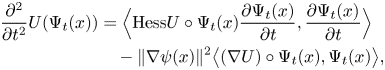
where the final term is zero since $\nabla U\circ \Psi _t(x)$ is in the tangent space at $\Psi _t(x)$
 , hence is perpendicular to $\Psi _t(x)$
 . We therefore have the crucial inequality

To simplify the function $K$ , we recall from [Reference Gradsteyn and Ryzhik9] 8.342 the Maclaurin series

where we have introduced Euler's $\Gamma$ function and Riemann's $\zeta$
 function, so

Now we consider (1.32) with the hypothesis (1.27) in force. The Carleman determinant contributes a nonnegative term as in (1.25), while the final integral in (1.32) combines with the integral of $K(\Vert \nabla \psi (x)\Vert )$ to give

When $\mu$ is normalized surface area, $U$
 is a constant and the hypothesis (1.27) holds with $\kappa _U=1$
 .
.
2. Transportation on compact Riemannian manifolds
Let $M$ be a connected, compact and $C^\infty$
 smooth Riemannian manifold of dimension $n$
 without boundary, and let $g$
 be the Riemannian metric tensor, giving metric $d$
 . Let $\mu ({\rm d}x)=e^{-U(x)}{\rm d}x$
 be a probability measure on $M$
 where ${\rm d}x$
 is Riemannian measure and $U\in C^2(M; {\bf R})$
 . Suppose that $\nu$
 is a probability measure on $M$
 that is of finite relative entropy with respect to $\mu$
 . Then by McCann's theory [Reference McCann12], there exists a Lipschitz function $\psi :M\rightarrow {\bf R}$
 such that $\Psi (x)=\exp _x(\nabla \psi (x))$
 induces $\nu$
 from $\mu$
 . then we let $\Psi _t(x)=\exp _x(t\nabla \psi (x))$
 . We proceed to compute quantities which we need for our extension of lemma 1.2.
Given distinct points $x,\,y\in M$ , we suppose that $x=\exp _y(\xi )$
 , and for $w\in T_yM$
 introduce
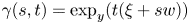
so that $t\mapsto \gamma (s,\,t)$ is a geodesic, and in particular $\gamma (0,\,t)$
 is the geodesic from $y=\gamma (0,\,0)$
 to $x=\gamma (0,\,1)$
 . When $y=\exp _x(\nabla \psi (x))$
 for a Lipschitz function $\psi :M\rightarrow {\bf R}$
 , we can determine $\xi$
 as follows. Let $\phi (z)=-\psi (z)$
 and introduce its infimal convolution

which is attained at $x$ since $y=\exp _x(\nabla \psi (x))=\exp _x(-\nabla \phi (x))$
 . Now $\phi ^{cc}(x)=\phi (x)$
 , so
, so

where the infimum is attained at $y$ since $\phi (x)+\phi ^c(y)=d(x,\,y)^2/2$
 . By lemma 2 of [Reference McCann12], $\phi ^c$
 is Lipschitz and

The speed of $\gamma (0,\,t)$ is given by

Let $R$ be the curvature of the Levi–Civita derivation $\nabla$
 so
so

Then by [Reference Pedersen13] p 36, for all $Y\in T_xM$ , the curvature operator $R_Y: X\mapsto R(X,\,Y)Y$
 is self-adjoint with respect to the scalar product on $T_xM$
 . Also

satisfies the initial conditions
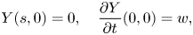
and Jacobi's differential equation [Reference Chavel4] (2.43)

By calculating the first variation of the length formula [Reference Pedersen13] p 161, one shows that
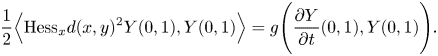
Assume that there are no conjugate points on $\gamma (s,\,t)$ . Then by varying $w$
 , we can make $Y(0,\,1)$
 cover a neighbourhood of $0$
 in $T_xM$
 . Let
. Let

and

Let $J_{\exp _x}(v)$ be the Jacobian of the map $T_xM\rightarrow M$
 given by $v\mapsto \exp _x(v)$
 , as in (3.4) of [Reference Cabre3].
Lemma 2.1 Suppose that $\Psi _t (x)=\exp _x(t \nabla \psi (x))$ , where $\Psi _1$
 induces the probability measure $\nu$
 from $\mu$
 and gives the optimal transport map for the $W_2$
 metric. Then the relative entropy satisfies

where $H$ is symmetric and $A+H$
 is also positive definite. If $\psi \in C^2(M; {\bf R})$
 , then equality holds in (2.12).
Proof. This is similar to lemma 1.2. As in (1.5), we have

and by standard calculations [Reference Pedersen13] p 32 we have

since $\Psi _t(x)$ is a geodesic.
The curvature operator is the symmetic operator $R_Z:Y\mapsto R(Z,\,Y)Z$ . If $M$
 has nonnegative Ricci curvature so that $R_Z\geq 0$
 as a matrix for all $Z$
 , then we have

by (3.4) of [Ca].
The following result recovers the Lichnérowicz integral, as in (4.16) of [Reference Blower1] and (1.1) of [Reference Deuschel and Stroock7]. This integral also appears implicitly in the Hessian calculations in appendix D of [Reference Lott and Villani11]. Let $\Vert H\Vert _{HS}$ be the Hilbert–Schmidt norm of $H$
 .
.
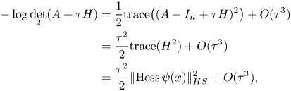
Proposition 2.2 Suppose that $\psi \in C^2(M; {\bf R})$ and $\Psi _\tau (x)=\exp _x(\tau \nabla \psi (x))$
 induces a probability measure $\nu _\tau$
 from $\mu$
 such that $\Psi _\tau$
 is the optimal transport map for the $W_2$
 metric. Then

Proof. For small $\tau >0$ , we rescale $\psi$
 to $\tau \psi$
 and consider $y=\exp _x(\tau \nabla \psi (x))$
 ; then we return to $x$
 along a geodesic $\gamma _\tau (t)=\exp _y(-t\nabla (-\tau \psi )^c(y))$
 for $0\leq t\leq 1$
 with constant speed $\tau \Vert \nabla \psi (x)\Vert$
 . Observe that $\tau \psi (x)=(-\tau \psi )^c(y)-\tau ^2\Vert \nabla \psi (x)\Vert ^2/2$
 , and $\nabla _xd(x,\,y)^2/2=-\exp _x^{-1}(y)=-\tau \nabla \psi (x)$
 and $\nabla _yd(x,\,y)^2/2=-\exp _y^{-1}(x)=\nabla (-\tau \psi )^c(y)$
 by Gauss's Lemma. Recalling that the curvature operator is self-adjoint by page 36 of [Reference Pedersen13], we choose the basis of $T_yM$
 so that the first basis vector points along the direction of the geodesic $\gamma _\tau (0)$
 . Hence Jacobi's equation (2.8) can be expressed as a second-order differential equation in block matrix form, with a symmetric matrix $S_{-\nabla (-\tau \psi )^c(y)}$
 given by components of the curvature tensor such that

as in (2.4) of [Reference Cordero-Erausquin, McCann and Schmuckensläger6]. Then the Jacobi equation reduces to a first-order block matrix equation with blocks of shape $(1+(n-1))\times (1+(n-1))$ in a $(2n)\times (2n)$
 matrix

To find the limit as $\tau \rightarrow 0$ , we can assume that $S_{-\nabla (-\tau \psi )^c (y)}$
 is constant on the geodesic, and may be expressed as $\tau ^2 S$
 where $\tau ^2 S=S_{\tau \nabla \psi (x)}$
 has shape ${(n-1)\times (n-1)}$
 . The functions $\cos \alpha$
 and $\sin \alpha /\alpha$
 are entire and even, so $\cos \sqrt {s}$
 and $\sin \sqrt {s}/\sqrt {s}$
 are entire functions, hence they operate on complex matrices. Note that the matrix

in the bottom left corner is symmetric, has rank less than or equal to $n-1$ , and does not depend upon $t$
 . Hence we consider the matrix

which has derivative

so we can use this formula to solve (2.18). So the approximate differential equation has solution

Hence by (2.9) we have

which gives rise to the approximation

and likewise we obtain

From (2.19), we have
so the result follows by lemma 2.1.
We conclude with a transportation inequality which generalizes proposition 1.3 to the unit spheres ${\bf S}^n$ . See [Reference Blower and Bolley2] for a discussion of measures on product spaces.
Theorem 2.3 Let $M={\bf S}^n$ for some $n\geq 2,$
 and suppose that

for some $\kappa _U>0$ . Then

Proof. In this case, the curvature operator is constant, so we have $S_{\nabla \psi (x)} Y=\Vert \nabla \psi (x)\Vert ^2Y$ , so
, so

Thus the result follows with a similar proof to proposition 1.3 using data from the proof of proposition 2.2.
Acknowledgments
I thank Graham Jameson for helpful remarks concerning inequalities which led to (1.34). I am also grateful to the referee, whose helpful comments improved the exposition.

 Open access