


1. Introduction
In a planetary system each orbiting body is deformed by the gravity of the massive central primary. For an orbiting body in the system, this deformation gives rise to a quadrupole moment in its mass distribution subject to periodic torques from the central body (Murray & Dermott Reference Murray and Dermott1999). The component of torque along the rotation axis of the orbiting body causes a periodic modulation to its rotation rate that is known as forced longitudinal libration (Comstock & Bills Reference Comstock and Bills2003). As a consequence of the quadrupole mass moment, there exist resonant configurations for certain orbits where the mean rotation rate, $\Omega _0$
, of the orbiting body is an integer or half-integer multiple of its mean motion,
$\Omega _0$
, of the orbiting body is an integer or half-integer multiple of its mean motion, $n$
(Murray & Dermott Reference Murray and Dermott1999). An orbiting body locked in a 1:1 spin-orbit resonance in a circular orbit has its equatorial long axis aligned with the direction of the central body in equilibrium; in this case, the orbiting body experiences no torque. However, for the same spin-orbit resonance, but in an elliptical orbit, the variation of the orbital velocity causes a periodic misalignment of the long axis which implies a torque with a leading-order frequency equal to the mean motion (Comstock & Bills Reference Comstock and Bills2003). For a spin-orbit configuration characterised by
$n$
(Murray & Dermott Reference Murray and Dermott1999). An orbiting body locked in a 1:1 spin-orbit resonance in a circular orbit has its equatorial long axis aligned with the direction of the central body in equilibrium; in this case, the orbiting body experiences no torque. However, for the same spin-orbit resonance, but in an elliptical orbit, the variation of the orbital velocity causes a periodic misalignment of the long axis which implies a torque with a leading-order frequency equal to the mean motion (Comstock & Bills Reference Comstock and Bills2003). For a spin-orbit configuration characterised by $p=\Omega _0/n$
not equal to unity, forced librations occur at the frequency
$p=\Omega _0/n$
not equal to unity, forced librations occur at the frequency $2(p-1)n$
even in a circular orbit (Comstock & Bills Reference Comstock and Bills2003); for Mercury
$2(p-1)n$
even in a circular orbit (Comstock & Bills Reference Comstock and Bills2003); for Mercury $(p=3/2)$
the leading-order forced longitudinal libration frequency is equal to the orbital mean motion.
$(p=3/2)$
the leading-order forced longitudinal libration frequency is equal to the orbital mean motion.
Some planetary bodies contain global fluid layers being either subsurface oceans encased in a shell of ice, as is the case for several outer solar system moons, or molten cores encased in rocky mantles. The solid shell librates alone on top of the internal fluid layer (e.g. Van Hoolst et al. Reference Van Hoolst, Rambaux, Kratekin and Baland2009), leading to a differential motion at the fluidsolid boundary. Drag forces cause the mechanical transfer of rotational energy from the mantle (ice shell) to the outer core (ocean) where it is dissipated. Broadly, the exchange of energy is mediated by three coupling mechanisms (e.g. Le Bars et al. Reference Le Bars, Cébron and Le Gal2015). Viscous coupling refers to the influence of friction at the fluidsolid boundary. Topographical coupling is the pressure interaction that results at points along the boundary where the latter is moving along its own local normal direction; for longitudinal libration topographical coupling only occurs in a non-axisymmetric container. Finally, magnetic coupling is also possible in cases when a magnetic field permeates an electrically conducting fluid core, and if the lowermost mantle is at least weakly electrically conducting.
In a fluid rotating with angular velocity $\Omega _0$
, the Coriolis acceleration acts as the restoring force for transverse ‘inertial’ waves with oscillation frequencies in the range
$\Omega _0$
, the Coriolis acceleration acts as the restoring force for transverse ‘inertial’ waves with oscillation frequencies in the range $(0,2\Omega _0)$
. Inertial waves exhibit a special dispersion relation that links their frequency to the direction of their wave vector (e.g. Greenspan Reference Greenspan1968; Le Bars et al. Reference Le Bars, Cébron and Le Gal2015; Tilgner Reference Tilgner2015). In a contained rotating fluid, inertial waves can coalesce to form normal modes that store energy in the constructive interference patterns formed by the waves at specific frequencies (Greenspan Reference Greenspan1968). The natural frequencies and distributions of the modal velocity and pressure fields are determined by the shape of the container. In a spherical domain the analytical form of these normal modes were first presented by Bryan (Reference Bryan1889); for discussions of the details of these structures see Kudlick (Reference Kudlick1966), Greenspan (Reference Greenspan1968), Zhang et al. (Reference Zhang, Liao and Earnshaw2004), Zhang & Liao (Reference Zhang and Liao2017) and Ivers et al. (Reference Ivers, Jackson and Winch2015).
$(0,2\Omega _0)$
. Inertial waves exhibit a special dispersion relation that links their frequency to the direction of their wave vector (e.g. Greenspan Reference Greenspan1968; Le Bars et al. Reference Le Bars, Cébron and Le Gal2015; Tilgner Reference Tilgner2015). In a contained rotating fluid, inertial waves can coalesce to form normal modes that store energy in the constructive interference patterns formed by the waves at specific frequencies (Greenspan Reference Greenspan1968). The natural frequencies and distributions of the modal velocity and pressure fields are determined by the shape of the container. In a spherical domain the analytical form of these normal modes were first presented by Bryan (Reference Bryan1889); for discussions of the details of these structures see Kudlick (Reference Kudlick1966), Greenspan (Reference Greenspan1968), Zhang et al. (Reference Zhang, Liao and Earnshaw2004), Zhang & Liao (Reference Zhang and Liao2017) and Ivers et al. (Reference Ivers, Jackson and Winch2015).
Longitudinal librations can excite inertial modes, as was studied experimentally by Aldridge & Toomre (Reference Aldridge and Toomre1969) and Aldridge (Reference Aldridge1972) and numerically by Rieutord (Reference Rieutord1991) in both rotating spheres and spherical shells. Although it is often the case that a spherical shell is more representative of the geometry of the fluid envelope of a planet, there is no known method to extend the analytical representations of the inertial modes in a full sphere to a spherical shell domain. A focusing effect occurs in certain geometries including the spherical shell (e.g. Maas & Lam Reference Maas and Lam1995; Rieutord & Valdettaro Reference Rieutord and Valdettaro1997; Tilgner Reference Tilgner1999) because the angle between the wave vector and the rotation axis is conserved when an inertial wave reflects at a boundary (Phillips Reference Phillips1963). Analytical forms of the inviscid inertial modes in the spherical domain are possible because of the ideal shape of the container while for more general geometries such as the spherical shell, inviscid solutions, aside from those purely toroidal fields, typically exhibit singular behaviour (Rieutord et al. Reference Rieutord, Georgeot and Valdettaro2001).
In the case of a longitudinally librating, electrically insulating spherical container, the mechanical forcing is communicated to the fluid exclusively by viscous coupling. In planetary applications the Ekman number $E$
, which characterises the strength of viscous forces relative to the Coriolis force, is of the order of
$E$
, which characterises the strength of viscous forces relative to the Coriolis force, is of the order of $10^{-10}$ $10^{-15}$
. The influence of viscosity can be taken into account asymptotically which leads to a boundary layer of thickness proportional to
$10^{-15}$
. The influence of viscosity can be taken into account asymptotically which leads to a boundary layer of thickness proportional to $E^{1/2}$
as described by Ekman (Reference Ekman1905). The boundary layer flow drives a mass flux in the direction normal to the boundary; the amplitude of this flux is also proportional to
$E^{1/2}$
as described by Ekman (Reference Ekman1905). The boundary layer flow drives a mass flux in the direction normal to the boundary; the amplitude of this flux is also proportional to $E^{1/2}$
and this radial forcing can excite the inertial modes in the bulk of the interior of the sphere when the system is driven at the appropriate frequency (Greenspan Reference Greenspan1968). The inertial mode flow in the bulk induces patterns of lateral fluid motion that modify the structure of the boundary layer from below, leading to an adjustment in the Ekman flux that effectively damps the mode (e.g. Zhang & Liao Reference Zhang and Liao2017; Lin et al. Reference Lin, Hollerbach, Noir and Vantieghem2023). Since the damping and forcing effects of the radial Ekman flux are both proportional to
$E^{1/2}$
and this radial forcing can excite the inertial modes in the bulk of the interior of the sphere when the system is driven at the appropriate frequency (Greenspan Reference Greenspan1968). The inertial mode flow in the bulk induces patterns of lateral fluid motion that modify the structure of the boundary layer from below, leading to an adjustment in the Ekman flux that effectively damps the mode (e.g. Zhang & Liao Reference Zhang and Liao2017; Lin et al. Reference Lin, Hollerbach, Noir and Vantieghem2023). Since the damping and forcing effects of the radial Ekman flux are both proportional to $E^{1/2}$
, the resulting excitation amplitude is independent of
$E^{1/2}$
, the resulting excitation amplitude is independent of $E$
in the limit
$E$
in the limit $E \rightarrow 0$
as was explained by Zhang et al. (Reference Zhang, Chan, Liao and Aurnou2013). This is in contrast to the case of topographic forcing where the modes receive direct pressure forcing from the boundary while the damping due to their Ekman layer is still proportional to
$E \rightarrow 0$
as was explained by Zhang et al. (Reference Zhang, Chan, Liao and Aurnou2013). This is in contrast to the case of topographic forcing where the modes receive direct pressure forcing from the boundary while the damping due to their Ekman layer is still proportional to $E^{1/2}$
. This leads to a resonant modal amplitude proportional to
$E^{1/2}$
. This leads to a resonant modal amplitude proportional to $E^{-1/2}$
as demonstrated by Zhang et al. (Reference Zhang, Chan and Liao2012) for the case of an oblate spheroid librating in latitude (see also Vantieghem et al. (Reference Vantieghem, Cébron and Noir2015)).
$E^{-1/2}$
as demonstrated by Zhang et al. (Reference Zhang, Chan and Liao2012) for the case of an oblate spheroid librating in latitude (see also Vantieghem et al. (Reference Vantieghem, Cébron and Noir2015)).
The existing studies of planetary flows forced by longitudinal libration are largely focused on identifying the conditions for turbulent instability (Noir et al. Reference Noir, Hemmerlin, Wicht, Baca and Aurnou2009; Calkins et al. Reference Calkins, Noir, Eldredge and Aurnou2010; Zhang et al. Reference Zhang, Chan and Liao2011; Cébron et al. Reference Cébron, Le Bars, Noir and Aurnou2012; Wu & Roberts Reference Wu and Roberts2013; Grannan et al. Reference Grannan, Lebars, Cébron and Aurnou2014; Favier et al. Reference Favier, Grannan, Le Bars and Aurnou2015; Lemasquerier et al. Reference Lemasquerier, Grannan, Vidal, Cébron, Favier, Le Bars and Aurnou2017; Le Reun et al. Reference Le Reun, Favier and Le Bars2019), the structure of the nonlinear mean zonal flow (Busse Reference Busse2010; Sauret et al. Reference Sauret, Cébron, Morize and Le Bars2010; Noir et al. Reference Noir, Cébron, Le Bars, Sauret and Aurnou2012; Sauret & Le Dizès Reference Sauret and Le Dizès2012; Cébron et al. Reference Cébron, Vidal, Schaeffer, Borderies and Sauret2021; Lin & Noir Reference Lin and Noir2021), computing the resonant amplitudes of the driven inertial modes (Zhang et al. Reference Zhang, Chan, Liao and Aurnou2013; Lin et al. Reference Lin, Hollerbach, Noir and Vantieghem2023), or scrutinising the structure of the wave attractors in a spherical shell (Rieutord & Valdettaro Reference Rieutord and Valdettaro2018; Lin & Noir Reference Lin and Noir2021; He et al. Reference He, Favier, Rieutord and Le Dizès2022, Reference He, Favier, Rieutord and Le Dizès2023). The flow driven by viscous coupling in a longitudinally librating planet is a mechanism for dissipation, it draws rotational energy from the mantle (ice shell) enclosing the outer core (ocean). This energy is dissipated as heat in the bulk fluid possibly helping to maintain a subsurface ocean in a liquid state. Furthermore, this dissipation will play a role in the evolution of planetary orbits through spin-orbit coupling (Murray & Dermott Reference Murray and Dermott1999; Le Bars et al. Reference Le Bars, Lacaze, Le Dizés, Le Gal and Rieutord2010; Cébron et al. Reference Cébron, Le Bars, Noir and Aurnou2012). If the fluid is conducting and the driven flow in the bulk is destabilised it can even contribute to dynamo action (Le Bars et al. Reference Le Bars, Wieczorek, Karatekin, Cébron and Laneuville2011; Wu & Roberts Reference Wu and Roberts2013; Le Bars et al. Reference Le Bars, Cébron and Le Gal2015).
The viscous dissipation associated with inertial modes is well understood in the context of the generic eigenvalue problem (e.g. Greenspan Reference Greenspan1968; Zhang et al. Reference Zhang, Liao and Earnshaw2004; Rieutord & Valdettaro Reference Rieutord and Valdettaro2018). However, their influence on the dissipation in forced longitudinal libration has yet to be extensively studied. Rekier et al. (Reference Rekier, Trinh, Triana and Dehant2019) presented numerical findings on the influence of inertial waves on dissipation in a longitudinally librating spherical shell, however, they only addressed a limited parameter range focused on the physical case of Enceladus. Cébron et al. (Reference Cébron, Laguerre, Noir and Schaeffer2019) studied dissipation in the flow forced by viscous coupling in a related problem, that of a precessing spherical shell, although they focused on the potential for dynamo action in the nonlinear regime. Likewise, dissipation has been studied in the case of flows driven by tidal forcing by Ogilvie (Reference Ogilvie2005, Reference Ogilvie2009), Rieutord & Valdettaro (Reference Rieutord and Valdettaro2010), Rovira-Navarro et al. (Reference Rovira-Navarro, Rieutord, Gerkema, Maas, van der Wal and Vermeersen2019) and Lin & Ogilvie (Reference Lin and Ogilvie2021) for example. All of these studies highlighted the role of inertial waves in enhancing diffusion. In particular, Lin & Ogilvie (Reference Lin and Ogilvie2021) showed that, although their presence may be obscured by the influence of wave attractors, global eigenmode structures can still be excited by tidal forcing in the spherical shell, as they are in a full sphere or spheroid. We therefore believe that insight can be gained into the role of inertial waves in dissipation by studying the case of the full sphere in detail through the use of the available explicit representations of the inertial modes. Another motivation for studying the general subject of resonating full sphere inertial modes is their detection in the convective cores of main sequence stars through resonances with gravito-inertial modes in the surrounding radiative envelope (Ouazzani et al. Reference Ouazzani, Lignières, Dupret, Salmon, Ballot, Christophe and Takata2020).
Here, we investigate the viscous dissipation in a fluid, rotating sphere that is induced by longitudinal libration of its surface. We examine the properties of the analytical and numerical solutions to the linearised fluid equations for this problem which is applicable to the case of weak amplitude libration. We limit our attention to solutions of the linearised problem. The nonlinear response of the rotating fluid sphere to longitudinal libration of its boundary surface is multifaceted. At larger forcing amplitude the Ekman layer becomes centrifugally unstable (e.g. Noir et al. Reference Noir, Hemmerlin, Wicht, Baca and Aurnou2009; Calkins et al. Reference Calkins, Noir, Eldredge and Aurnou2010). Moreover, it is well known (e.g. Busse Reference Busse2010; Sauret et al. Reference Sauret, Cébron, Morize and Le Bars2010; Noir et al. Reference Noir, Cébron, Le Bars, Sauret and Aurnou2012; Sauret & Le Dizès Reference Sauret and Le Dizès2012; Cébron et al. Reference Cébron, Vidal, Schaeffer, Borderies and Sauret2021; Lin & Noir Reference Lin and Noir2021) that nonlinear interactions can generate a mean flow, largely a differential rotation, as well as small oscillations at frequencies corresponding to the higher harmonics of the forcing frequency (Koch et al. Reference Koch, Harlander and Hollerbach2013). Furthermore, in a general geometry attractors and focusing can produce localised nonlinear effects (e.g. Le Dizès Reference Le Dizès2020; Boury et al. Reference Boury, Sibgatullin, Ermanyuk, Shmakova, Odier, Joubaud, Maas and Dauxois2021) in the limit $E \rightarrow 0$
. It is outside the scope of this work to explore how such nonlinear interactions contribute to a change in the dissipation. By focusing on the linear problem, we can establish a general lower bound on the viscous dissipation as a function of frequency. This should then assist future studies targeting dissipation in the nonlinear regime.
$E \rightarrow 0$
. It is outside the scope of this work to explore how such nonlinear interactions contribute to a change in the dissipation. By focusing on the linear problem, we can establish a general lower bound on the viscous dissipation as a function of frequency. This should then assist future studies targeting dissipation in the nonlinear regime.
In the linear regime the dissipation induced by the Ekman boundary layer flow scales as $E^{1/2}$
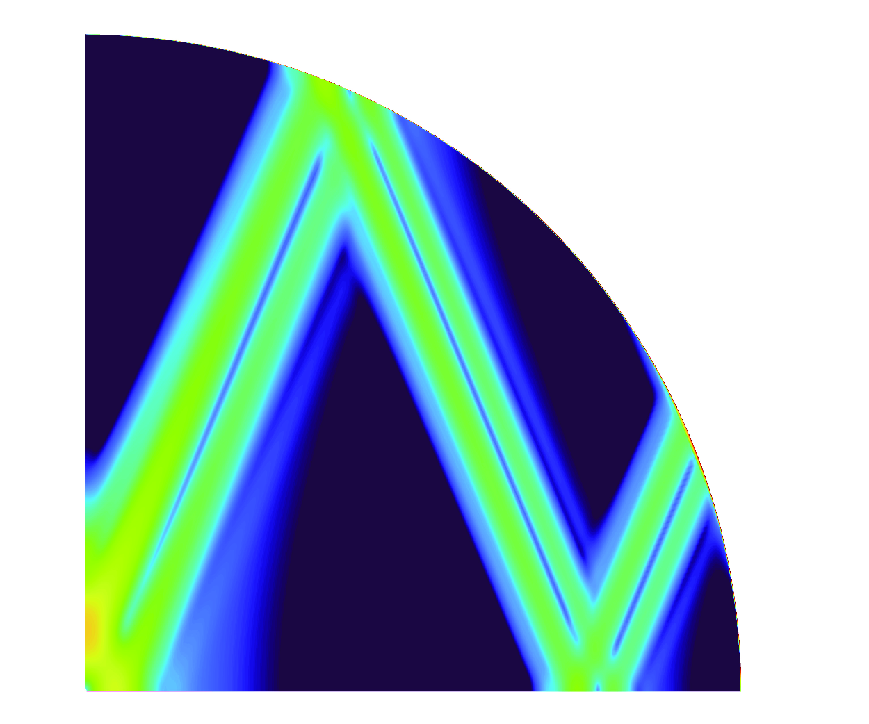
(Cébron et al. Reference Cébron, Laguerre, Noir and Schaeffer2019). As highlighted by the recent study of Lin et al. (Reference Lin, Hollerbach, Noir and Vantieghem2023), the kinetic energy of the flow in the interior peaks at discrete frequencies that match those of the inertial modes, but it is minimised at frequencies that match those of wave attractors focused in conic shear layers. The primary question we want to address is how these interior flows alter the global dissipation of energy in the context of the forced problem. To do so, we use both analytical and numerical methods.
$E^{1/2}$
(Cébron et al. Reference Cébron, Laguerre, Noir and Schaeffer2019). As highlighted by the recent study of Lin et al. (Reference Lin, Hollerbach, Noir and Vantieghem2023), the kinetic energy of the flow in the interior peaks at discrete frequencies that match those of the inertial modes, but it is minimised at frequencies that match those of wave attractors focused in conic shear layers. The primary question we want to address is how these interior flows alter the global dissipation of energy in the context of the forced problem. To do so, we use both analytical and numerical methods.
Our study is organised as follows. In § 2.1 we formulate the system of linear partial differential equations of the hydrodynamics problem and present the expressions of the kinetic energy and dissipation. In § 2.2 we provide an overview of the semi-spectral numerical method we use to compute our solutions. In § 2.3, we derive an analytical solution of the amplitude of a given inertial mode driven by longitudinal libration. The solution is based on a matched asymptotic approach. A similar approach was used by Zhang et al. (Reference Zhang, Chan, Liao and Aurnou2013); Lin et al. (Reference Lin, Hollerbach, Noir and Vantieghem2023) although their results are restricted to the resonant amplitude when the forcing frequency exactly matches the natural frequency of a mode. We extend this analytical solution to all frequencies in the range of $(0,2\Omega _0)$
. Furthermore we present expressions for the dissipation and kinetic energy of the boundary layer alone as a function of forcing frequency that are accurate to leading order in
$(0,2\Omega _0)$
. Furthermore we present expressions for the dissipation and kinetic energy of the boundary layer alone as a function of forcing frequency that are accurate to leading order in $E$
. This allows us to further understand theoretical aspects of the spectrum of kinetic energy and dissipation in the linear regime. In 2.4 we briefly review how shear layers can develop in the sphere volume at certain frequencies. Results are presented in § 3, followed by a discussion and a summary of conclusions (§ 4).
$E$
. This allows us to further understand theoretical aspects of the spectrum of kinetic energy and dissipation in the linear regime. In 2.4 we briefly review how shear layers can develop in the sphere volume at certain frequencies. Results are presented in § 3, followed by a discussion and a summary of conclusions (§ 4).
2. Theory
2.1. Formulation of the linearised libration forcing problem
Consider a sphere, $S$
, of radius
$S$
, of radius $R$
and volume
$R$
and volume $V$
, filled with an incompressible fluid of uniform density and temperature rotating with angular velocity
$V$
, filled with an incompressible fluid of uniform density and temperature rotating with angular velocity $\Omega _0$
about a fixed axis
$\Omega _0$
about a fixed axis $\boldsymbol {\hat {e}}_z$
. The rotation axis defines the pole of the spherical-polar coordinate system
$\boldsymbol {\hat {e}}_z$
. The rotation axis defines the pole of the spherical-polar coordinate system $(r,\theta ,\varphi )$
where
$(r,\theta ,\varphi )$
where $r$
is the radius, and
$r$
is the radius, and $\theta$
and
$\theta$
and $\varphi$
are colatitude and longitude, respectively. The amplitude of the angular velocity of the spherical container,
$\varphi$
are colatitude and longitude, respectively. The amplitude of the angular velocity of the spherical container, $\Omega _S$
, is perturbed by a harmonic oscillation about
$\Omega _S$
, is perturbed by a harmonic oscillation about $\Omega _0$
of the form
$\Omega _0$
of the form
 \begin{align} \Omega _S(t) &= \Omega _0(1+\varepsilon \cos (\Omega _0 \lambda t)), \end{align}
where $\varepsilon \ll 1$
and
$\varepsilon \ll 1$
and $0 \lt \lambda \lt 2$
are the amplitude and frequency of the oscillation, respectively, and
$0 \lt \lambda \lt 2$
are the amplitude and frequency of the oscillation, respectively, and $t$
is time. In what follows, all quantities are non-dimensionalised using the length scale
$t$
is time. In what follows, all quantities are non-dimensionalised using the length scale $R$
and the time scale
$R$
and the time scale $\Omega _0^{-1}$
.
$\Omega _0^{-1}$
.
In the reference frame rotating with (dimensional) angular velocity $\Omega _0\boldsymbol {\hat {e}}_z$
, the velocity of the fluid,
$\Omega _0\boldsymbol {\hat {e}}_z$
, the velocity of the fluid, $\boldsymbol {u}$
, obeys the momentum equation
$\boldsymbol {u}$
, obeys the momentum equation
 \begin{align} \frac {\partial \boldsymbol {u}}{\partial t} + \boldsymbol {u} \boldsymbol {\cdot } \boldsymbol {\nabla } \boldsymbol {u} + 2\boldsymbol {\hat {e}}_z \times \boldsymbol {u} + \boldsymbol {\nabla } P = E\boldsymbol {\nabla }^2\boldsymbol {u}, \end{align}
where $P$
is the reduced pressure that includes the centrifugal force, and the Ekman number
$P$
is the reduced pressure that includes the centrifugal force, and the Ekman number $E$
is given by
$E$
is given by
 \begin{align} E = \frac {\nu }{\Omega _0 R^2}, \end{align}
where $\nu$
is the kinematic viscosity of the fluid.
$\nu$
is the kinematic viscosity of the fluid.
The motion of the fluid is also subject to incompressible mass conservation
 \begin{align} \boldsymbol {\nabla }\boldsymbol {\cdot } \boldsymbol {u} = 0, \end{align}
and the following no-slip and non-penetration conditions at the surface, $S$
of the spherical container
$S$
of the spherical container
 \begin{align} \boldsymbol {\hat {e}}_\varphi \boldsymbol {\cdot } \boldsymbol {u}|_S &= \varepsilon \sin \theta \cos (\lambda t), \end{align}
 \begin{align} \boldsymbol {\hat {e}}_\theta \boldsymbol {\cdot } \boldsymbol {u}|_S &= 0, \end{align}
 \begin{align} \boldsymbol {\hat {e}}_r \boldsymbol {\cdot } \boldsymbol {u}|_S &= 0, \end{align}
where $\boldsymbol {\hat {e}}_r$
,
$\boldsymbol {\hat {e}}_r$
, $\boldsymbol {\hat {e}}_\theta$
and
$\boldsymbol {\hat {e}}_\theta$
and $\boldsymbol {\hat {e}}_\varphi$
are the unit vectors of the spherical coordinate system.
$\boldsymbol {\hat {e}}_\varphi$
are the unit vectors of the spherical coordinate system.
The nonlinear term in equation 2.2 is second order in $\varepsilon$
, which provides the basis for ignoring its effects in the limit of weak forcing. Admittedly, the nonlinear term may still become locally important even for quite weak forcing due, for example, to shear layers associated with inertial wave attractors in the limit
$\varepsilon$
, which provides the basis for ignoring its effects in the limit of weak forcing. Admittedly, the nonlinear term may still become locally important even for quite weak forcing due, for example, to shear layers associated with inertial wave attractors in the limit $E \rightarrow 0$
. Nonlinear effects contributing to enhanced dissipation in these regions could render the linear estimates invalid even for very weak forcing when the Ekman number is taken to be small enough. In all, determining a threshold forcing amplitude associated with the onset of nonlinearities in the these flows in the limit
$E \rightarrow 0$
. Nonlinear effects contributing to enhanced dissipation in these regions could render the linear estimates invalid even for very weak forcing when the Ekman number is taken to be small enough. In all, determining a threshold forcing amplitude associated with the onset of nonlinearities in the these flows in the limit $E \rightarrow 0$
is a formidable task which lies outside the scope of this work.
$E \rightarrow 0$
is a formidable task which lies outside the scope of this work.
Because of the harmonic time dependence of the boundary condition (equation 2.5), we restrict our attention to oscillatory solutions with harmonic periodicity and do not attempt to capture any transient fluid motions resulting from a particular set of initial conditions. In this limit, we seek solutions that have the form of complex phasors with frequency $\lambda$
 \begin{align} \boldsymbol {u}(\boldsymbol {r},t) &= \frac {1}{2} \left ( \boldsymbol {q}(\boldsymbol {r}) e^{\mathrm {i}\lambda t} + \boldsymbol {q}^\dagger (\boldsymbol {r}) e^{-\mathrm {i}\lambda t}\right ), \end{align}
 \begin{align} P(\boldsymbol {r},t) &= \frac {1}{2} \left ( \phi (\boldsymbol {r}) e^{\mathrm {i}\lambda t} + \phi ^\dagger (\boldsymbol {r}) e^{-\mathrm {i}\lambda t} \right ), \end{align}
where the spatial parts of the solution given by $\boldsymbol {q}$
and
$\boldsymbol {q}$
and $\phi$
may be complex valued and
$\phi$
may be complex valued and $\dagger$
represents complex conjugation. By substituting this ansatz into equations 2.2, 2.4, and 2.5 and neglecting the nonlinear term, we write the equivalent equations of motion in terms of spatial variables alone and parametrised by the forcing frequency,
$\dagger$
represents complex conjugation. By substituting this ansatz into equations 2.2, 2.4, and 2.5 and neglecting the nonlinear term, we write the equivalent equations of motion in terms of spatial variables alone and parametrised by the forcing frequency,
 \begin{align} \mathrm {i} \lambda \boldsymbol {q} + 2 \boldsymbol {\hat {e}}_z \times \boldsymbol {q} + \boldsymbol {\nabla } \phi &= E\boldsymbol {\nabla }^2 \boldsymbol {q}, \end{align}
 \begin{align} \boldsymbol {\nabla } \boldsymbol {\cdot } \boldsymbol {q} & = 0, \end{align}
subject to the following conditions at the surface of the spherical container:
 \begin{align} \boldsymbol {\hat {e}}_\varphi \boldsymbol {\cdot } \boldsymbol {q}|_S &= \varepsilon \sin \theta , \end{align}
 \begin{align} \boldsymbol {\hat {e}}_\theta \boldsymbol {\cdot } \boldsymbol {q}|_S &= 0, \end{align}
 \begin{align} \boldsymbol {\hat {e}}_r \boldsymbol {\cdot }\boldsymbol {q}|_S &= 0. \end{align}
To consider the energy budget of the linearised system, we take the scalar product of $\boldsymbol {u}$
with equation 2.2. Neglecting the nonlinear term, integrating over the volume
$\boldsymbol {u}$
with equation 2.2. Neglecting the nonlinear term, integrating over the volume $V$
of the fluid, using the divergence theorem and taking into account equations 2.4 and 2.5c
leads to the following power relation:
$V$
of the fluid, using the divergence theorem and taking into account equations 2.4 and 2.5c
leads to the following power relation:
 \begin{align} \frac {{\rm d}\mathcal {K}}{{\rm d}t} = \mathcal {P} - \mathcal {D}, \end{align}
where $\mathcal {K}$
is the net kinetic energy of the fluid,
$\mathcal {K}$
is the net kinetic energy of the fluid, $\mathcal {P}$
is the power transferred into the fluid region by viscous stresses at the librating boundary, and
$\mathcal {P}$
is the power transferred into the fluid region by viscous stresses at the librating boundary, and $\mathcal {D}$
is the dissipation in the bulk of the fluid. In terms of the velocity field, they are expressed as
$\mathcal {D}$
is the dissipation in the bulk of the fluid. In terms of the velocity field, they are expressed as
 \begin{align} \mathcal {K} &= \int _V \frac {1}{2} |\boldsymbol {u}|^2, \end{align}
 \begin{align} \mathcal {P} &= E\int _S (\boldsymbol {u} \boldsymbol {\otimes } \boldsymbol {\hat {e}}_r) \boldsymbol {:} ( \boldsymbol {\boldsymbol {\nabla } u} + \boldsymbol { \boldsymbol {\nabla } u}^T), \end{align}
 \begin{align} \mathcal {D} &= E\int _V \boldsymbol {\nabla } \boldsymbol {u} \boldsymbol {:} (\boldsymbol {\nabla } \boldsymbol {u} + \boldsymbol {\nabla } \boldsymbol {u}^T), \end{align}
where $\boldsymbol {\otimes }$
is the outer product and
$\boldsymbol {\otimes }$
is the outer product and $\boldsymbol {:}$
denotes the full contraction of two second rank tensors.
$\boldsymbol {:}$
denotes the full contraction of two second rank tensors.
Let us denote the integral time average of a quantity over a libration period, $2\pi/\lambda$
, that begins at an arbitrary time
$2\pi/\lambda$
, that begins at an arbitrary time $t_0$
by
$t_0$
by
 \begin{align} \langle \boldsymbol {\cdot } \rangle = \frac {\lambda }{2\pi} \int _{t_0}^{t_0+2\pi/\lambda }\, \boldsymbol {\cdot } \, {\rm d}t. \end{align}
Since we restrict our attention to perfectly oscillatory solutions, the left hand side of equation 2.9 vanishes under time averaging since
 \begin{align} \left \langle \frac {{\rm d} \mathcal {K}}{{\rm d}t}\right \rangle = \frac {\lambda }{2\pi} \int _{t_0}^{t_0+2\pi/\lambda } \frac {{\rm d}\mathcal {K}}{{\rm d}t}{\rm d}t = \frac {\lambda }{2\pi} \left [ \mathcal {K}|_{t_0+2\pi/\lambda } - \mathcal {K}|_{t_0}\right ] = 0. \end{align}
Then the time-average of equation 2.9 leads to the relation
 \begin{align} \langle \mathcal {P} \rangle = \langle \mathcal {D} \rangle , \end{align}
which states that for oscillatory solutions there must be equilibrium between the energy added into the system and the energy dissipated in the bulk over the course of a libration period. This assumes that the surface $S$
has been librating at the same amplitude and frequency for a sufficiently long time that any transient fluid motion due to different conditions in the past has attenuated.
$S$
has been librating at the same amplitude and frequency for a sufficiently long time that any transient fluid motion due to different conditions in the past has attenuated.
2.2. Numerical solution of the linear problem
To compute numerical solutions to equation 2.7, we use the following decomposition of the velocity field $\boldsymbol {q}$
(e.g. Tilgner Reference Tilgner1999):
$\boldsymbol {q}$
(e.g. Tilgner Reference Tilgner1999):
 \begin{equation} \boldsymbol {q} = \boldsymbol {\nabla } \times (\boldsymbol {\nabla } \times (W \boldsymbol {\hat {e}}_r)) + \boldsymbol {\nabla } \times (Z\boldsymbol {\hat {e}}_r), \end{equation}
where $W$
and
$W$
and $Z$
are the scalar poloidal and toroidal potential fields respectively; this expansion automatically ensures that
$Z$
are the scalar poloidal and toroidal potential fields respectively; this expansion automatically ensures that $\boldsymbol {q}$
satisfies mass conservation (equation 2.7b
). The scalar potentials are expanded as a summation of fully normalised surface spherical harmonics
$\boldsymbol {q}$
satisfies mass conservation (equation 2.7b
). The scalar potentials are expanded as a summation of fully normalised surface spherical harmonics $Y_\ell ^m$
of degree
$Y_\ell ^m$
of degree $\ell$
and order
$\ell$
and order $m$
$m$
 \begin{align} W(r) &= \sum _{\ell = 1}^{\ell _{\text {max.}}} \sum _{m=-\ell }^\ell W_{\ell }^m(r) Y_\ell ^m(\theta ,\varphi ), \end{align}
 \begin{align} Z(r) &= \sum _{\ell = 1}^{\ell _{\text {max.}}} \sum _{m=-\ell }^\ell Z_{\ell }^m(r) Y_\ell ^m(\theta ,\varphi ), \end{align}
where $W_\ell ^m(r)$
and
$W_\ell ^m(r)$
and $Z_\ell ^m(r)$
are numerical coefficient functions and where
$Z_\ell ^m(r)$
are numerical coefficient functions and where
 \begin{equation} \int _0^{2\pi} \int _0^{\pi} Y_\ell ^m(\theta ,\varphi ) Y_{\ell '}^{m'}(\theta ,\varphi )^\dagger \sin \theta \, d\theta \, d\varphi = \delta _{\ell \ell '}\delta _{mm'}. \end{equation}
By taking the operations $\boldsymbol {e}_r \boldsymbol {\cdot } \boldsymbol {\nabla } \times$
and
$\boldsymbol {e}_r \boldsymbol {\cdot } \boldsymbol {\nabla } \times$
and $\boldsymbol {e}_r \boldsymbol {\cdot } \boldsymbol {\nabla } \times (\boldsymbol {\nabla } \times )$
on equation 2.7a
, then substituting the decomposition (equation 2.14) into the resulting equations and making use of equation 2.16 we obtain at each radius
$\boldsymbol {e}_r \boldsymbol {\cdot } \boldsymbol {\nabla } \times (\boldsymbol {\nabla } \times )$
on equation 2.7a
, then substituting the decomposition (equation 2.14) into the resulting equations and making use of equation 2.16 we obtain at each radius $r$
and for each distinct pair
$r$
and for each distinct pair $(\ell ,m)$
(see Rieutord Reference Rieutord1987)
$(\ell ,m)$
(see Rieutord Reference Rieutord1987)
 \begin{align} A_\ell ^m Z_\ell ^m &= C_\ell ^m W_{\ell -1}^m + D_{\ell }^m W_{\ell +1}^m, \end{align}
 \begin{align} A_\ell ^m B_\ell ^m W_\ell ^m &= C_\ell ^m Z_{\ell -1}^m + D_{\ell }^m Z_{\ell +1}^m, \end{align}
where $A_\ell ^m$
,
$A_\ell ^m$
, $B_\ell ^m$
,
$B_\ell ^m$
, $C_\ell ^m$
and
$C_\ell ^m$
and $D_\ell ^m$
are operators defined by
$D_\ell ^m$
are operators defined by
 \begin{align} A_\ell ^m &= \mathrm {i}(\ell (\ell +1) \lambda - 2m) + \ell (\ell +1) E B_{\ell }^m, \end{align}
 \begin{align} B_\ell ^m &= \left ( \frac {\ell (\ell +1)}{r^2} - \frac {d^2}{{\rm d}r^2}\right ), \end{align}
 \begin{align} C_\ell ^m &= 2(\ell -1)(\ell +1) \sqrt {\frac {(\ell -m)(\ell +m)}{(2\ell - 1)(2\ell +1)}} \left [ \frac {d}{{\rm d}r} - \frac {\ell }{r}\right ] , \end{align}
 \begin{align} D_\ell ^m &= 2\ell (\ell +2) \sqrt {\frac {(\ell +1 -m)(\ell +1 +m)}{(2\ell +1)(2\ell +3)}} \left [ \frac {d}{{\rm d}r} + \frac {\ell +1}{r}\right ]. \end{align}
Written in terms of $W_\ell ^m$
and
$W_\ell ^m$
and $Z_\ell ^m$
, the boundary conditions (equation 2.8) on the spherical surface at
$Z_\ell ^m$
, the boundary conditions (equation 2.8) on the spherical surface at $r = 1$
are given by
$r = 1$
are given by
 \begin{align} \left . Z_\ell ^m \right |_S &= \varepsilon \sqrt {\frac {4\pi}{3}} \delta _{\ell 1}\delta _{m0}, \end{align}
 \begin{align} \left . W_\ell ^m \right |_S &= 0 \ \text {for all } \ell , m, \end{align}
 \begin{align} \left . \frac {{\rm d}W_\ell ^m}{{\rm d}r} \right |_S &= 0\ \text {for all } \ell , m. \end{align}
Due to symmetry the system of equations 2.17 decouples across spherical harmonic order. Since longitudinal libration involves a purely axisymmetric forcing, we restrict our attention to zonal coefficients with $m = 0$
. Upon close examination, the structure of the system of equations 2.17 implies that only those zonal toroidal coefficients
$m = 0$
. Upon close examination, the structure of the system of equations 2.17 implies that only those zonal toroidal coefficients $Z_\ell ^0$
of odd degree and poloidal coefficients
$Z_\ell ^0$
of odd degree and poloidal coefficients $W_\ell ^0$
of even degree are non-zero in the solution; these modes comprise the equatorially symmetric part of the field
$W_\ell ^0$
of even degree are non-zero in the solution; these modes comprise the equatorially symmetric part of the field $\boldsymbol {q}$
. The set of zonal coefficients of reverse symmetry comprise the equatorially anti-symmetric part of the solution which vanishes due to the equatorial symmetry of the forcing. Equations 2.17 can therefore be structured formally as the following tri-diagonal matrix system
$\boldsymbol {q}$
. The set of zonal coefficients of reverse symmetry comprise the equatorially anti-symmetric part of the solution which vanishes due to the equatorial symmetry of the forcing. Equations 2.17 can therefore be structured formally as the following tri-diagonal matrix system

where the symbol $\hat {Z}_1^0$
is a place holder for the term that arises due to the libration forcing boundary condition, the exact form of which is determined by the choice of radial discretisation.
$\hat {Z}_1^0$
is a place holder for the term that arises due to the libration forcing boundary condition, the exact form of which is determined by the choice of radial discretisation.
To solve the system of ordinary differential equations (ODEs), we use a second-order finite difference scheme on a radial grid of $N$
Chebyshev like points that are modified by the nonlinear scaling suggested by Lin et al. (Reference Lin, Hollerbach, Noir and Vantieghem2023)
$N$
Chebyshev like points that are modified by the nonlinear scaling suggested by Lin et al. (Reference Lin, Hollerbach, Noir and Vantieghem2023)
 \begin{equation} r_k = \cos \left ( \frac {\pi}{2} \frac {k}{N}\right ) \left [ 1 + 0.45 \sin ^2\left ( \frac {\pi}{2} \frac {k}{N}\right ) \right ] , k = 0,1,\dots ,N-1. \end{equation}
This choice of radial grid concentrates the points in the thin boundary layer. Once discretised, the system is solved directly by Gaussian elimination. Additional considerations are necessary to ensure regularity of the solution at the origin; although they use a spectral approach for the radial discretisation, Lin et al. (Reference Lin, Hollerbach, Noir and Vantieghem2023) provides relevant information on this subject as well as further references.
Let $N$
denote the number of radial grid points used in the discretisation, while
$N$
denote the number of radial grid points used in the discretisation, while $\ell _{max.}$
denotes the maximal spherical harmonic degree used in the solution. The resolution that is necessary to sufficiently converge the numerical solution depends strongly on
$\ell _{max.}$
denotes the maximal spherical harmonic degree used in the solution. The resolution that is necessary to sufficiently converge the numerical solution depends strongly on $E$
. Lower values of
$E$
. Lower values of $E$
demand that an increasingly small boundary layer be resolved. As such, in our calculations we found a resolution of
$E$
demand that an increasingly small boundary layer be resolved. As such, in our calculations we found a resolution of $N = 160$
,
$N = 160$
, $\ell _{max.} = 80$
was sufficient for
$\ell _{max.} = 80$
was sufficient for $E = 10^{-4}-10^{-5}$
, while
$E = 10^{-4}-10^{-5}$
, while $N = 250$
and
$N = 250$
and $\ell _{max.} = 180$
for
$\ell _{max.} = 180$
for $E = 10^{-6} - 10^{-7}$
, and finally
$E = 10^{-6} - 10^{-7}$
, and finally $N = 350$
,
$N = 350$
, $\ell _{max.} = 250$
was used for
$\ell _{max.} = 250$
was used for $E = 10^{-8}$
. At these resolutions all computations were practical on a regular PC, to access even lower values of
$E = 10^{-8}$
. At these resolutions all computations were practical on a regular PC, to access even lower values of $E$
numerically, the required resolution demands a larger amount of memory than is typical for a regular PC.
$E$
numerically, the required resolution demands a larger amount of memory than is typical for a regular PC.
The linearised approach is valid for $\varepsilon \ll 1$
. The nonlinear perturbations to the linearised solution that arise from its self interaction scale with
$\varepsilon \ll 1$
. The nonlinear perturbations to the linearised solution that arise from its self interaction scale with $\varepsilon ^2$
, but the dependence on
$\varepsilon ^2$
, but the dependence on $E$
has not been extensively explored. At larger forcing amplitude the Ekman layer becomes centrifugally unstable (e.g. Noir et al. Reference Noir, Hemmerlin, Wicht, Baca and Aurnou2009; Calkins et al. Reference Calkins, Noir, Eldredge and Aurnou2010). Numerical results reported by Calkins et al. (Reference Calkins, Noir, Eldredge and Aurnou2010) for libration with a rotating spherical shell show that Taylor–Görtler vortices form at first in the equatorial region when
$E$
has not been extensively explored. At larger forcing amplitude the Ekman layer becomes centrifugally unstable (e.g. Noir et al. Reference Noir, Hemmerlin, Wicht, Baca and Aurnou2009; Calkins et al. Reference Calkins, Noir, Eldredge and Aurnou2010). Numerical results reported by Calkins et al. (Reference Calkins, Noir, Eldredge and Aurnou2010) for libration with a rotating spherical shell show that Taylor–Görtler vortices form at first in the equatorial region when $\varepsilon \gt 46E^{1/2}$
, however, these results are not necessarily valid below
$\varepsilon \gt 46E^{1/2}$
, however, these results are not necessarily valid below $E = 10^{-6}$
. At lower Ekman numbers the influence of the nonlinearities may be significant in localised regions like those associated with attractors (Boury et al. Reference Boury, Sibgatullin, Ermanyuk, Shmakova, Odier, Joubaud, Maas and Dauxois2021) for weaker forcing than the boundary layer stability criterion of Calkins et al. (Reference Calkins, Noir, Eldredge and Aurnou2010) suggests. In particular, nonlinear production of vorticity in these localised regions could have a significant influence on total dissipation even at low forcing amplitudes.
$E = 10^{-6}$
. At lower Ekman numbers the influence of the nonlinearities may be significant in localised regions like those associated with attractors (Boury et al. Reference Boury, Sibgatullin, Ermanyuk, Shmakova, Odier, Joubaud, Maas and Dauxois2021) for weaker forcing than the boundary layer stability criterion of Calkins et al. (Reference Calkins, Noir, Eldredge and Aurnou2010) suggests. In particular, nonlinear production of vorticity in these localised regions could have a significant influence on total dissipation even at low forcing amplitudes.
2.3. Approximate solution by matched asymptotics
In this section we construct an approximate analytical solution to the linearised problem (equation 2.7). Motivated by the smallness of $E$
and following the general approach of Greenspan (Reference Greenspan1968), we seek an asymptotic solution to equation 2.7 that has the form
$E$
and following the general approach of Greenspan (Reference Greenspan1968), we seek an asymptotic solution to equation 2.7 that has the form
 \begin{align} \boldsymbol {q} &= \boldsymbol {q}_0 + \boldsymbol {q}_1 E^{1/2} + \boldsymbol {q}_2 E + \mathcal {O}(E^{3/2}), \end{align}
 \begin{align} \phi &= \phi _0 + \phi _1 E^{1/2} + \phi _2 E + \mathcal {O}(E^{3/2}). \end{align}
We then deal with the solution to each term separately. The leading-order terms, $\boldsymbol {q}_0$
,
$\boldsymbol {q}_0$
, $\phi _0$
as well as the first-order correction terms,
$\phi _0$
as well as the first-order correction terms, $\boldsymbol {q}_1$
,
$\boldsymbol {q}_1$
, $\phi _1$
satisfy the inviscid momentum equation asymptotically
$\phi _1$
satisfy the inviscid momentum equation asymptotically
 \begin{align} \mathrm {i} \lambda ( \boldsymbol {q}_0 +E^{1/2} \boldsymbol {q}_1) + 2 \boldsymbol {\hat {e}}_z \times (\boldsymbol {q}_0+E^{1/2} \boldsymbol {q}_1) + \boldsymbol {\nabla } (\phi _0 +E^{1/2} \phi _1)= \mathcal {O}(E). \end{align}
It is well known (e.g. Greenspan Reference Greenspan1968; Zhang et al. Reference Zhang, Liao and Earnshaw2004; Kida Reference Kida2011; Lin et al. Reference Lin, Hollerbach, Noir and Vantieghem2023) that equation 2.24 is an overdetermined problem when subject to both no-slip and non-penetration boundary conditions (equation 2.8). This necessitates the existence of a boundary layer solution that is introduced as follows:
 \begin{align} \boldsymbol {q} &= \boldsymbol {b}_0 +\boldsymbol {\psi }_0+ (\boldsymbol {b}_1+\boldsymbol {\psi }_1) E^{1/2} + (\boldsymbol {b}_2+\boldsymbol {\psi }_2) E+ \mathcal {O}(E^{3/2}), \end{align}
 \begin{align} \phi &= \phi _{b0}+\phi _{\psi 0} + (\phi _{b1}+\phi _{\psi 1})E^{1/2} + (\phi _{b2}+\phi _{\psi 2}) E + \mathcal {O}(E^{3/2}). \end{align}
The part denoted by $\boldsymbol {b}$
,
$\boldsymbol {b}$
, $\phi _b$
is the solution in the interior region which satisfies equation 2.24 and
$\phi _b$
is the solution in the interior region which satisfies equation 2.24 and $\boldsymbol {\psi }$
,
$\boldsymbol {\psi }$
, $\phi _\psi$
is the solution in the boundary layer.
$\phi _\psi$
is the solution in the boundary layer.
2.3.1. Ekman boundary layers
The boundary layer expansion is handled by the introduction of a stretched boundary layer coordinate (e.g. Zhang et al. Reference Zhang, Liao and Earnshaw2004)
 \begin{align} \xi = \frac {1-r}{E^{1/2}}. \end{align}
Furthermore, it is assumed that the gradients of boundary layer quantities are $\mathcal {O}(E^{-1/2})$
in the normal (radial) direction and
$\mathcal {O}(E^{-1/2})$
in the normal (radial) direction and $\mathcal {O}(1)$
in the lateral directions
$\mathcal {O}(1)$
in the lateral directions
 \begin{align} \frac {\partial \boldsymbol {\psi }}{\partial r} = - E^{-1/2} \frac {\partial \boldsymbol {\psi }}{\partial \xi } = \mathcal {O}(E^{-1/2}), \frac {\partial \boldsymbol {\psi }}{\partial \theta },\, \frac {\partial \boldsymbol {\psi }}{\partial \varphi } = \mathcal {O}(1). \end{align}
These assumptions lead to the following greatly simplified version of equation 2.7 that is accurate to leading order in the boundary layer (e.g. Ekman Reference Ekman1905)
 \begin{align} \mathrm {i} \lambda (\boldsymbol {\hat {e}}_\theta \boldsymbol {\cdot } \boldsymbol {\psi }_0) - 2 (\boldsymbol {\hat {e}}_\varphi \boldsymbol {\cdot } \boldsymbol {\psi }_0) \cos \theta &= \frac {\partial ^2(\boldsymbol {\hat {e}}_\theta \boldsymbol {\cdot } \boldsymbol {\psi }_0)}{\partial \xi ^2}, \end{align}
 \begin{align} \mathrm {i}\lambda (\boldsymbol {\hat {e}}_\varphi \boldsymbol {\cdot } \boldsymbol {\psi }_0) + 2 (\boldsymbol {\hat {e}}_\theta \boldsymbol {\cdot } \boldsymbol {\psi }_0) \cos \theta &= \frac {\partial ^2(\boldsymbol {\hat {e}}_\varphi \boldsymbol {\cdot } \boldsymbol {\psi }_0)}{\partial \xi ^2}. \end{align}
If the lateral motion of the boundary layer at the surface $S$
is specified by an arbitrary vector field
$S$
is specified by an arbitrary vector field $\boldsymbol {v}$
with
$\boldsymbol {v}$
with $\boldsymbol {\hat {e}}_r \boldsymbol {\cdot } \boldsymbol {v} \equiv 0$
, then the solution to equations 2.29 that satisfies the no-slip condition on
$\boldsymbol {\hat {e}}_r \boldsymbol {\cdot } \boldsymbol {v} \equiv 0$
, then the solution to equations 2.29 that satisfies the no-slip condition on $S$
with respect to this lateral motion is given by
$S$
with respect to this lateral motion is given by
 \begin{align} \begin{split} \boldsymbol {\Psi }_0\{\boldsymbol {v}\} &= \frac {1}{2} \left ( \mathcal {C}_+\{\boldsymbol {v}\} \exp (-\gamma _+ \xi ) + \mathcal {C}_-\{\boldsymbol {v}\} \exp (-\gamma _-\xi )\right ) \boldsymbol {\hat {e}}_\theta ,\\& + \frac {1}{2\mathrm {i}} \left ( \mathcal {C}_+\{\boldsymbol {v}\} \exp (-\gamma _+ \xi ) - \mathcal {C}_-\{\boldsymbol {v}\} \exp (-\gamma _-\xi )\right ) \boldsymbol {\hat {e}}_\varphi , \end{split} \end{align}
where
 \begin{align} \mathcal {C}_\pm \{\boldsymbol {v}\} &=( \boldsymbol {\hat {e}}_\theta \boldsymbol {\cdot } \boldsymbol {v})\pm \mathrm {i} (\boldsymbol {\hat {e}}_\varphi \boldsymbol {\cdot }\boldsymbol {v} ), \end{align}
 \begin{align} \gamma _\pm &= \sqrt {|\lambda \pm 2\cos \theta |} \exp \left ( \mathrm {i}\frac {\pi}{4} \text {sign}\{\lambda \pm 2 \cos \theta \}\right ). \end{align}
Moreover, the $\mathcal {O}(E^{1/2})$
radial Ekman pumping at the bottom of the boundary layer is derived from mass conservation (
$\mathcal {O}(E^{1/2})$
radial Ekman pumping at the bottom of the boundary layer is derived from mass conservation ( $\boldsymbol {\nabla } \boldsymbol {\cdot }( \boldsymbol {\psi }_0 +E^{1/2}\boldsymbol {\psi }_1)= 0$
)
$\boldsymbol {\nabla } \boldsymbol {\cdot }( \boldsymbol {\psi }_0 +E^{1/2}\boldsymbol {\psi }_1)= 0$
)
 \begin{align} \begin{split} &\Phi _1\{\boldsymbol {v}\}(\theta ,\varphi ) :=\lim _{\xi \rightarrow \infty } (\boldsymbol {\hat {e}}_r \boldsymbol {\cdot } \boldsymbol {\psi }_1(\xi ;\theta ,\varphi ))\\&= \frac {1}{\sin \theta }\int _0^\infty \left ( \frac {\partial (\boldsymbol {\hat {e}}_\theta \boldsymbol {\cdot } \boldsymbol {\Psi }_0\{\boldsymbol {v}\}(\xi ';\theta ,\varphi ) \sin \theta )}{\partial \theta } + \frac {\partial (\boldsymbol {\hat {e}}_\varphi \boldsymbol {\cdot } \boldsymbol {\Psi }_0\{\boldsymbol {v}\}(\xi ';\theta ,\varphi ))}{\partial \varphi }\right ) d \xi '. \end{split} \end{align}
The Ekman pumping is evaluated for the general solution (equation 2.30) for an arbitrary lateral forcing $\boldsymbol {v}$
to yield
$\boldsymbol {v}$
to yield
 \begin{align} \Phi _1\{\boldsymbol {v}\} = \frac {1}{2\sin \theta }\left [ \frac {\partial }{\partial \theta } \left ( \sin \theta \left ( \frac {\mathcal {C}_+\{\boldsymbol {v}\}}{\gamma _+} + \frac {\mathcal {C}_-\{\boldsymbol {v}\}}{\gamma _-}\right ) \right )-\mathrm {i}\frac {\partial }{\partial \varphi } \left ( \frac {\mathcal {C}_+\{\boldsymbol {v}\}}{\gamma _+} - \frac {\mathcal {C}_-\{\boldsymbol {v}\}}{\gamma _-}\right ) \right ]. \end{align}
For longitudinal librations, taking $\boldsymbol {v} = \sin \theta \boldsymbol {\hat {e}}_\varphi$
in equations 2.30 and 2.33 yields
$\boldsymbol {v} = \sin \theta \boldsymbol {\hat {e}}_\varphi$
in equations 2.30 and 2.33 yields
 \begin{align} \begin{split} \boldsymbol {\Psi }_0\{\sin \theta \boldsymbol {\hat {e}}_\varphi \} &= -\frac {\sin \theta }{2\mathrm {i}}\left ( \exp (-\gamma _+ \xi ) - \exp (-\gamma _- \xi )\right ) \boldsymbol {\hat {e}}_\theta \\& + \frac {\sin \theta }{2} \left ( \exp (-\gamma _+ \xi ) + \exp (-\gamma _-\xi )\right ) \boldsymbol {\hat {e}}_\varphi , \end{split} \end{align}
 \begin{align} \Phi _1\{ \sin \theta \boldsymbol {\hat {e}}_\varphi \} &= -\frac {1}{2 \mathrm {i}\sin \theta } \frac {\partial }{\partial \theta } \left ( \sin ^2\theta \left (\frac {1}{\gamma _+} -\frac {1}{\gamma _-}\right )\right ). \\[6pt] \nonumber \end{align}
Equations 2.34 comprise the leading-order response in the boundary layer to the longitudinal libration motion of the surface $S$
with
$S$
with $\varepsilon = 1$
.
$\varepsilon = 1$
.
2.3.2. The interior region
Now we are equipped to address the interior flow $\boldsymbol {b}$
,
$\boldsymbol {b}$
, $\phi _b$
. By equations 2.24–2.26, and since the boundary layer component of the solution vanishes in the interior region, the leading-order term in the interior solution satisfies
$\phi _b$
. By equations 2.24–2.26, and since the boundary layer component of the solution vanishes in the interior region, the leading-order term in the interior solution satisfies
 \begin{align} \mathrm {i}\lambda \boldsymbol {b}_0 + 2 \boldsymbol {\hat {e}}_z \times \boldsymbol {b}_0 + \boldsymbol {\nabla } \phi _{b0} &= \mathcal {O}(E^{1/2}), \end{align}
 \begin{align} \boldsymbol {\nabla } \boldsymbol {\cdot } \boldsymbol {b}_0 &= \mathcal {O}(E^{1/2}), \end{align}
and the non-penetration condition on the sphere surface $S$
$S$
 \begin{align} \left .\boldsymbol {\hat {e}}_r \boldsymbol {\cdot } \boldsymbol {b}_0\right |_S = 0 . \end{align}
The solution of this system is a superposition of the inviscid inertial modes of the sphere (see Greenspan (Reference Greenspan1964); Ivers et al. (Reference Ivers, Jackson and Winch2015); Zhang & Liao (Reference Zhang and Liao2017) for details)
 \begin{align} \boldsymbol {b}_0 &= \sum _{\ell , k, m} \mathcal {A}_{\ell ,k,m} \boldsymbol {q}_{\ell ,k,m}, \end{align}
 \begin{align} \phi _{b0} &= \sum _{\ell , k, m} \mathcal {A}_{\ell ,k,m} \phi _{\ell ,k,m}, \end{align}
where $\mathcal {A}_{\ell ,k,m}$
are the amplitude coefficients of the modes and
$\mathcal {A}_{\ell ,k,m}$
are the amplitude coefficients of the modes and $\ell , k,m$
are the wavenumber indices in the notation of Greenspan (Reference Greenspan1968) of the eigenfunction solutions. The wavenumbers broadly control the spatial scales of the modes such that their volumetric damping under the influence of viscosity is proportional to
$\ell , k,m$
are the wavenumber indices in the notation of Greenspan (Reference Greenspan1968) of the eigenfunction solutions. The wavenumbers broadly control the spatial scales of the modes such that their volumetric damping under the influence of viscosity is proportional to $\ell ^2$
,
$\ell ^2$
, $k^2$
and
$k^2$
and $m^2$
. For sufficiently large wavenumbers it is possible for the volumetric damping to become outsised, such that
$m^2$
. For sufficiently large wavenumbers it is possible for the volumetric damping to become outsised, such that $\|\boldsymbol {\nabla }^2\boldsymbol {q}_{\ell ,k,m}\| \geqslant \mathcal {O}(E^{-1/2})$
, violating the assumption of approximately inviscid dynamics for the first-order correction to the interior flow,
$\|\boldsymbol {\nabla }^2\boldsymbol {q}_{\ell ,k,m}\| \geqslant \mathcal {O}(E^{-1/2})$
, violating the assumption of approximately inviscid dynamics for the first-order correction to the interior flow, $\boldsymbol {b}_1,\phi _{b1}$
(see equation 2.24). To construct a solution that is consistent with the asymptotic expansion (equation 2.26) where the viscous term is neglected in the
$\boldsymbol {b}_1,\phi _{b1}$
(see equation 2.24). To construct a solution that is consistent with the asymptotic expansion (equation 2.26) where the viscous term is neglected in the $\mathcal {O}(E^{1/2})$
interior solution, it is necessary to restrict the expansion to those inertial modes with
$\mathcal {O}(E^{1/2})$
interior solution, it is necessary to restrict the expansion to those inertial modes with $\ell ,k,m \ll \mathcal {O}(E^{-1/4})$
(see Zhang et al. Reference Zhang, Liao and Earnshaw2004). The high wavenumber modes play a negligible role in the solution since they have overwhelming volumetric dissipation which prevents them from ever attaining significant amplitude.
$\ell ,k,m \ll \mathcal {O}(E^{-1/4})$
(see Zhang et al. Reference Zhang, Liao and Earnshaw2004). The high wavenumber modes play a negligible role in the solution since they have overwhelming volumetric dissipation which prevents them from ever attaining significant amplitude.
The eigenfunctions $\boldsymbol {q}_{\ell ,k,m}$
,
$\boldsymbol {q}_{\ell ,k,m}$
, $\phi _{\ell ,k,m}$
each satisfy the inviscid equations
$\phi _{\ell ,k,m}$
each satisfy the inviscid equations
 \begin{align} \mathrm {i}\lambda _{\ell ,k,m} \boldsymbol {q}_{\ell ,k,m} + 2 \boldsymbol {\hat {e}}_z \times \boldsymbol {q}_{\ell ,k,m} + \boldsymbol {\nabla } \phi _{\ell ,k,m} &= 0, \end{align}
 \begin{align} \boldsymbol {\nabla } \boldsymbol {\cdot } \boldsymbol {q}_{\ell ,k,m} &=0, \end{align}
subject to non-penetration on the surface $S$
of the sphere
$S$
of the sphere
 \begin{align} \left . \boldsymbol {\hat {e}}_r \boldsymbol {\cdot }\boldsymbol {q}_{\ell ,k,m}\right |_S = 0. \end{align}
Although the eigenvalues lie in the range $-2 \lt \lambda _{\ell ,k,m}\lt 2$
, the distribution is symmetrical for zonal modes (
$-2 \lt \lambda _{\ell ,k,m}\lt 2$
, the distribution is symmetrical for zonal modes ( $m = 0$
), the only modes excited by longitudinal libration; that is, for each eigenvalue
$m = 0$
), the only modes excited by longitudinal libration; that is, for each eigenvalue $\lambda _{\ell ,k,0}$
, the value
$\lambda _{\ell ,k,0}$
, the value $-\lambda _{\ell ,k,0}$
is also an eigenvalue (corresponding to inertial waves travelling in the opposite direction). Moreover, the eigenvalues are all real valued. It is useful to note (Greenspan Reference Greenspan1968) that the pressure eigenfunctions satisfy on the surface of the sphere (only at
$-\lambda _{\ell ,k,0}$
is also an eigenvalue (corresponding to inertial waves travelling in the opposite direction). Moreover, the eigenvalues are all real valued. It is useful to note (Greenspan Reference Greenspan1968) that the pressure eigenfunctions satisfy on the surface of the sphere (only at $r= 1$
)
$r= 1$
)
 \begin{equation} \phi _{\ell ,k,m}|_S(\theta ,\varphi ) = \mathcal {N}_{\ell ,k,m} Y_\ell ^m(\theta ,\varphi ), \end{equation}
where $\mathcal {N}_{\ell ,k,m}$
is an arbitrary constant that depends on the choice of normalisation, and
$\mathcal {N}_{\ell ,k,m}$
is an arbitrary constant that depends on the choice of normalisation, and $Y_\ell ^m$
is a degree
$Y_\ell ^m$
is a degree $\ell$
and order-
$\ell$
and order- $m$
surface spherical harmonic. The expression of the surface pressure distribution in terms of
$m$
surface spherical harmonic. The expression of the surface pressure distribution in terms of $Y_\ell ^m$
provides a clear interpretation of the mode indices
$Y_\ell ^m$
provides a clear interpretation of the mode indices $\ell$
,
$\ell$
, $m$
. The third index,
$m$
. The third index, $k$
, takes a finite number of values for each pair
$k$
, takes a finite number of values for each pair $(\ell ,m)$
and selects the internal structure of the mode. Finally, it will be necessary in the solution to use the orthogonality of the inertial modes (Greenspan Reference Greenspan1964; Ivers et al. Reference Ivers, Jackson and Winch2015)
$(\ell ,m)$
and selects the internal structure of the mode. Finally, it will be necessary in the solution to use the orthogonality of the inertial modes (Greenspan Reference Greenspan1964; Ivers et al. Reference Ivers, Jackson and Winch2015)
 \begin{align} \int _V \boldsymbol {q}_{\ell ,k,m}\boldsymbol {\cdot } \boldsymbol {q}_{\ell ',k',m'}^\dagger = \delta _{\ell \ell '} \delta _{kk'} \delta _{mm'}\int _V |\boldsymbol {q}_{\ell ,k,m}|^2. \end{align}
This orthogonality relation implies that the amplitude of each eigenmode that appears in equation 2.37 is determined by the Fourier type integral
 \begin{align} \mathcal {A}_{\ell ,k,m} = \frac {1}{\int _{V} |\boldsymbol {q}_{\ell ,k,m}|^2}\int _V \boldsymbol {b}_0 \boldsymbol {\cdot } \boldsymbol {q}_{\ell ,k,m}^\dagger . \end{align}
The numerical values of the coefficients $\mathcal {A}_{\ell ,k,m}$
depend on the choice of normalisation for the inertial modes. In this work we shall always use the same normalisation as Zhang et al. (Reference Zhang, Liao and Earnshaw2004, Reference Zhang, Chan, Liao and Aurnou2013); Zhang & Liao (Reference Zhang and Liao2017) in order to facilitate direct comparison between results when possible. The normalisation is arbitrary and is designed to allow the simplest form of the inertial modes in spherical-polar coordinates. It is defined as follows for the zonal
$\mathcal {A}_{\ell ,k,m}$
depend on the choice of normalisation for the inertial modes. In this work we shall always use the same normalisation as Zhang et al. (Reference Zhang, Liao and Earnshaw2004, Reference Zhang, Chan, Liao and Aurnou2013); Zhang & Liao (Reference Zhang and Liao2017) in order to facilitate direct comparison between results when possible. The normalisation is arbitrary and is designed to allow the simplest form of the inertial modes in spherical-polar coordinates. It is defined as follows for the zonal $(m=0)$
and equatorially symmetric (
$(m=0)$
and equatorially symmetric ( $\ell$
even) modes
$\ell$
even) modes
 \begin{align} \begin{split} \int _V &|\boldsymbol {q}_{\ell ,k,0}|^2 = \sum _{i = 0}^{\ell /2} \sum _{j=0}^{\ell /2-i} \sum _{q=0}^{\ell /2} \sum _{n = 0}^{\ell /2-q} \left [ \frac {(-1)^{i+j+q+n}\pi }{2(2(i+j+q+n)+1)!!}\right ] \\& \times \left [ \frac {8iq(2i+2q-3)!!(j+n)!}{\lambda _{\ell ,k,0}^2} + \frac {jn(1+\lambda _{\ell ,k,0}^2/4)(2i+2q-1)!!(j+n-1)!}{(1-\lambda _{\ell ,k,0}^2/4)^2}\right ]\\& \times \left [ \left (\frac {\lambda _{\ell ,k,0}}{2}\right )^{2(i+q)} \frac {(1-\lambda _{\ell ,k,0}^2/4)^{j+n}(2(\ell /2+i+j)-1)!!(2(\ell /2+q+n)-1)!!}{(2i-1)!!(2q-1)!!(\ell /2-i-j)!(\ell /2-q-n)!i!q!(j!)^2(n!)^2}\right ], \end{split} \end{align}
where $(2i-1)!! = (2i-1)(2i-3)\dots (3)(1)$
and
$(2i-1)!! = (2i-1)(2i-3)\dots (3)(1)$
and $(-1)!! = 1$
and
$(-1)!! = 1$
and $(0)! = 1$
.
$(0)! = 1$
.
Libration forcing only excites those zonal modes with equatorial symmetry (even $\ell$
).
$\ell$
). $\ell = 4$
is the lowest degree at which a mode exists. For such modes the number of values taken by the index
$\ell = 4$
is the lowest degree at which a mode exists. For such modes the number of values taken by the index $k$
is
$k$
is $\ell /2-1$
, that is, for
$\ell /2-1$
, that is, for $\ell = 4$
there is only one mode
$\ell = 4$
there is only one mode $(4,1,0)$
, while for
$(4,1,0)$
, while for $\ell = 6$
there are two,
$\ell = 6$
there are two, $(6,1,0)$
and
$(6,1,0)$
and $(6,2,0)$
and so on. Let
$(6,2,0)$
and so on. Let $\ell _{\text {max.}}$
be the maximal modal degree excited to leading order in the expansion of
$\ell _{\text {max.}}$
be the maximal modal degree excited to leading order in the expansion of $\boldsymbol {b}_0$
. The total number of modes excited to leading order is then
$\boldsymbol {b}_0$
. The total number of modes excited to leading order is then
 \begin{equation} \mathcal {N}_{\text {excited}}=\frac {\ell _{\text {max.}}}{4}\left ( \frac {\ell _{\text {max.}}}{2}-1\right ). \end{equation}
Respecting the restriction of the expansion to low wavenumber modes we have $\ell _{max.} \ll \mathcal {O}(E^{-1/4})$
which implies that
$\ell _{max.} \ll \mathcal {O}(E^{-1/4})$
which implies that $\mathcal {N}_{\text {excited}} \ll \mathcal {O}(E^{-1/2})$
.
$\mathcal {N}_{\text {excited}} \ll \mathcal {O}(E^{-1/2})$
.
The objective is now to determine an expression for the modal coefficients, $\mathcal {A}_{\ell ,k,m}$
. Previous studies (e.g. Greenspan Reference Greenspan1968; Zhang et al. Reference Zhang, Chan, Liao and Aurnou2013; Lin et al. Reference Lin, Hollerbach, Noir and Vantieghem2023) have derived analytical expressions for the amplitude
$\mathcal {A}_{\ell ,k,m}$
. Previous studies (e.g. Greenspan Reference Greenspan1968; Zhang et al. Reference Zhang, Chan, Liao and Aurnou2013; Lin et al. Reference Lin, Hollerbach, Noir and Vantieghem2023) have derived analytical expressions for the amplitude $\mathcal {A}_{\ell ,k,m}$
of an individual inertial mode when the system is forced at precisely the resonant frequency
$\mathcal {A}_{\ell ,k,m}$
of an individual inertial mode when the system is forced at precisely the resonant frequency $\lambda _{\ell ,k,m}$
of that mode. Under this resonance condition, the amplitude
$\lambda _{\ell ,k,m}$
of that mode. Under this resonance condition, the amplitude $\mathcal {A}_{\ell ,k,m}$
driven purely by the Ekman pumping is independent of
$\mathcal {A}_{\ell ,k,m}$
driven purely by the Ekman pumping is independent of $E$
. The explanation of this phenomenon is as follows. When an inertial mode is excited to resonance the boundary layer flow must adjust to ensure that the no-slip condition remains satisfied. The adjustment of the boundary layer leads to an additional
$E$
. The explanation of this phenomenon is as follows. When an inertial mode is excited to resonance the boundary layer flow must adjust to ensure that the no-slip condition remains satisfied. The adjustment of the boundary layer leads to an additional $\mathcal {O}(E^{1/2})$
Ekman pumping that acts like a drag force on the mode, opposing the Ekman pumping induced by the viscous coupling, and thus damping the excitation. Because the damping and forcing are each
$\mathcal {O}(E^{1/2})$
Ekman pumping that acts like a drag force on the mode, opposing the Ekman pumping induced by the viscous coupling, and thus damping the excitation. Because the damping and forcing are each $\mathcal {O}(E^{1/2})$
, the excitation amplitude is then
$\mathcal {O}(E^{1/2})$
, the excitation amplitude is then $\mathcal {O}(1)$
, that is, independent of
$\mathcal {O}(1)$
, that is, independent of $E$
in the asymptotic limit.
$E$
in the asymptotic limit.
In the theoretical development by Greenspan (Reference Greenspan1968) the viscous damping of the inertial mode is derived separately from the forcing problem as a $\mathcal {O}(E^{1/2})$
correction to the natural frequency of the mode. The correction to the frequency adds an imaginary part scaling with
$\mathcal {O}(E^{1/2})$
correction to the natural frequency of the mode. The correction to the frequency adds an imaginary part scaling with $E^{1/2}$
that captures the damping. Then, separately, Greenspan (Reference Greenspan1968) derives an expression for the amplitude
$E^{1/2}$
that captures the damping. Then, separately, Greenspan (Reference Greenspan1968) derives an expression for the amplitude $\mathcal {A}_{\ell ,k,m}$
in the context of the forcing problem. This expression involves a term
$\mathcal {A}_{\ell ,k,m}$
in the context of the forcing problem. This expression involves a term $(\lambda - \lambda _{\ell ,k,m})$
on the denominator which seemingly produces a divergent amplitude if
$(\lambda - \lambda _{\ell ,k,m})$
on the denominator which seemingly produces a divergent amplitude if $\lambda _{\ell ,k,m} = \lambda$
. However, instead of using the real eigenvalue
$\lambda _{\ell ,k,m} = \lambda$
. However, instead of using the real eigenvalue $\lambda _{\ell ,k,m}$
, it is the
$\lambda _{\ell ,k,m}$
, it is the $\mathcal {O}(E^{1/2})$
correction that is substituted and its imaginary part means that
$\mathcal {O}(E^{1/2})$
correction that is substituted and its imaginary part means that $(\lambda - \lambda _{\ell ,k,m}) \neq 0$
for any real valued forcing frequency
$(\lambda - \lambda _{\ell ,k,m}) \neq 0$
for any real valued forcing frequency $\lambda$
; this leads to a finite resonance that is damped by viscosity.
$\lambda$
; this leads to a finite resonance that is damped by viscosity.
The approach used by both Zhang et al. (Reference Zhang, Chan, Liao and Aurnou2013) and Lin et al. (Reference Lin, Hollerbach, Noir and Vantieghem2023) is to treat the correction to the boundary layer flow induced by an inertial mode simultaneously to that which is induced by the viscous coupling to the laterally moving surface. Ultimately, they find the same result as Greenspan (Reference Greenspan1968) for the resonant amplitude of the inertial mode when $\lambda _{\ell ,k,m} = \lambda$
but without the added step of separately deriving the damping factor as a correction to the natural frequency of the mode.
$\lambda _{\ell ,k,m} = \lambda$
but without the added step of separately deriving the damping factor as a correction to the natural frequency of the mode.
Here, we use an approach that extends the techniques used by Lin et al. (Reference Lin, Hollerbach, Noir and Vantieghem2023) and Zhang et al. (Reference Zhang, Chan, Liao and Aurnou2013) to determine the leading-order amplitude of all inertial modes not only for $\lambda = \lambda _{\ell ,k,m}$
, but for a range of forcing frequencies in a window around each resonant peak. The correction to the boundary layer flow that is induced by the excitement of inertial modes is taken into account simultaneously to the boundary layer that forms in response to the libration of
$\lambda = \lambda _{\ell ,k,m}$
, but for a range of forcing frequencies in a window around each resonant peak. The correction to the boundary layer flow that is induced by the excitement of inertial modes is taken into account simultaneously to the boundary layer that forms in response to the libration of $S$
. Since the inertial modes are excited by the radial Ekman pumping, we turn our attention to the first-order correction
$S$
. Since the inertial modes are excited by the radial Ekman pumping, we turn our attention to the first-order correction $\boldsymbol {b}_1$
,
$\boldsymbol {b}_1$
, $\phi _{b1}$
in the expansion of equations 2.24–2.26, this
$\phi _{b1}$
in the expansion of equations 2.24–2.26, this $\mathcal {O}(E^{1/2})$
flow must match the
$\mathcal {O}(E^{1/2})$
flow must match the $\mathcal {O}(E^{1/2})$
Ekman pumping from the full boundary layer solution. This first-order correction satisfies the inviscid equations in the bulk
$\mathcal {O}(E^{1/2})$
Ekman pumping from the full boundary layer solution. This first-order correction satisfies the inviscid equations in the bulk
 \begin{align} \mathrm {i} \lambda \boldsymbol {b}_1 + 2 \boldsymbol {\hat {e}}_z \times \boldsymbol {b}_1 + \boldsymbol {\nabla } \phi _{b1} &= \mathcal {O}(E^{1/2}), \end{align}
 \begin{align} \boldsymbol {\nabla } \boldsymbol {\cdot } \boldsymbol {b}_1 &= \mathcal {O}(E^{1/2}), \end{align}
and the matching condition implies an inhomogeneous boundary condition on the surface $S$
$S$
 \begin{align} \left .\boldsymbol {\hat {e}}_r \boldsymbol {\cdot } \boldsymbol {b}_1\right |_S = \lim _{\xi \rightarrow \infty } \boldsymbol {\hat {e}}_r \boldsymbol {\cdot } \boldsymbol {\psi }_{1} = \Phi _1\{\boldsymbol {\psi }_0|_S\} .\end{align}
From equations 2.24–2.26 we infer that together, the leading-order interior solution $\boldsymbol {b}_0$
,
$\boldsymbol {b}_0$
, $\phi _{b0}$
and the first-order correction
$\phi _{b0}$
and the first-order correction $\boldsymbol {b}_1$
,
$\boldsymbol {b}_1$
, $\phi _{b1}$
satisfy the following equation in the interior region:
$\phi _{b1}$
satisfy the following equation in the interior region:
 \begin{align} \mathrm {i}\lambda (\boldsymbol {b}_0 + E^{1/2} \boldsymbol {b}_1) + 2 \boldsymbol {\hat {e}}_z \times ( \boldsymbol {b}_0 + E^{1/2} \boldsymbol {b}_1) + \boldsymbol {\nabla } ( \phi _0 + E^{1/2} \phi _1) = \mathcal {O}(E). \end{align}
The inertial mode expansion (equation 2.37) is substituted to equation 2.48 and use is made of the orthogonality of the modes (equation 2.41), we obtain, after algebraic manipulations, the following expression:
 \begin{align} \mathrm {i} (\lambda - \lambda _{\ell ,k,m})\left [ \mathcal {A}_{\ell ,k,m} + E^{1/2} \frac {\int _V \boldsymbol {b}_{1} \cdot \boldsymbol {q}_{\ell ,k,m}^\dagger }{\int _V |\boldsymbol {q}_{\ell ,k,m}|^2}\right ]= -\frac {E^{1/2}}{\int _V |\boldsymbol {q}_{\ell ,k,m}|^2} \int _S \phi _{\ell ,k,m}^\dagger (\boldsymbol {\hat {e}}_r \boldsymbol {\cdot } \boldsymbol {b}_1) + \mathcal {O}(E). \end{align}
The details of the derivation of this expression are given in Appendix A. Note that equation 2.49 links the coefficients, $\mathcal {A}_{\ell ,k,m}$
of the inertial mode expansion of
$\mathcal {A}_{\ell ,k,m}$
of the inertial mode expansion of $\boldsymbol {b}_0$
(equation 2.37) to the matching condition (equation 2.47) involving the correction
$\boldsymbol {b}_0$
(equation 2.37) to the matching condition (equation 2.47) involving the correction $\boldsymbol {b}_1$
.
$\boldsymbol {b}_1$
.
Now that the link between the Ekman pumping and the modal coefficients of the leading-order solution is established, we turn our attention to the no-slip boundary condition and libration forcing that determine the Ekman pumping itself. The no-slip boundary condition on the surface $S$
(equation 2.8) for the leading-order terms implies
$S$
(equation 2.8) for the leading-order terms implies
 \begin{align} \left . \boldsymbol {b}_0\right |_S + \left .\boldsymbol {\psi _0} \right |_S = \varepsilon \sin \theta \boldsymbol {\hat {e}}_\varphi + \mathcal {O}(E^{1/2}). \end{align}
Substituting the inertial mode expansion of $\boldsymbol {b}_0$
(equation 2.37) the leading-order boundary layer solution
$\boldsymbol {b}_0$
(equation 2.37) the leading-order boundary layer solution $\boldsymbol {\psi }_0$
must obey the boundary condition
$\boldsymbol {\psi }_0$
must obey the boundary condition
 \begin{align} \left . \boldsymbol {\psi }_0\right |_S = \varepsilon \sin \theta \boldsymbol {\hat {e}}_\varphi - \sum _{\ell ,k,m} \mathcal {A}_{\ell ,k,m} \boldsymbol {q}_{\ell ,k,m}|_S. \end{align}
Because the governing equations 2.29 are linear, the solution can be written as follows:
 \begin{align} \boldsymbol {\psi }_0 = \varepsilon \boldsymbol {\Psi }_0\{ \sin \theta \boldsymbol {\hat {e}}_\varphi \} - \sum _{\ell ,k,m} \mathcal {A}_{\ell ,k,m} \boldsymbol {\Psi }_0\{\boldsymbol {q}_{\ell ,k,m}|_S\}, \end{align}
where $\boldsymbol {\Psi }_0\{\sin \theta \boldsymbol {\hat {e}}_\varphi \}$
is given by equation 2.34a
.
$\boldsymbol {\Psi }_0\{\sin \theta \boldsymbol {\hat {e}}_\varphi \}$
is given by equation 2.34a
.
Each part of the solution in equation 2.52 induces a radial Ekman pumping
 \begin{align} \Phi _1\{\boldsymbol {\psi }_0|_S\} = \lim _{\xi \rightarrow \infty } ( \boldsymbol {\hat {e}}_r \boldsymbol {\cdot } \boldsymbol {\psi }_1 )= \varepsilon \Phi _1\{\sin \theta \boldsymbol {\hat {e}}_\varphi \} - \sum _{\ell ,k,m} \mathcal {A}_{\ell ,k,m} \Phi _1\{\boldsymbol {q}_{\ell ,k,m}|_S\}, \end{align}
where $\Phi _1\{\sin \theta \boldsymbol {\hat {e}}_\varphi \}$
is given by equation 2.34b
. By substituting equation 2.53 into equation 2.49 using the matching condition (equation 2.47) we obtain
$\Phi _1\{\sin \theta \boldsymbol {\hat {e}}_\varphi \}$
is given by equation 2.34b
. By substituting equation 2.53 into equation 2.49 using the matching condition (equation 2.47) we obtain
 \begin{align} \begin{split} &\mathrm {i} (\lambda - \lambda _{\ell ,k,m})\left [ \mathcal {A}_{\ell ,k,m} + E^{1/2} \frac {\int _V \boldsymbol {b}_{1} \cdot \boldsymbol {q}_{\ell ,k,m}^\dagger }{\int _V |\boldsymbol {q}_{\ell ,k,m}|^2}\right ] - E^{1/2} \sum _{\ell ',k',m'} \mathcal {A}_{\ell ',k',m'}\mathcal {S}_{\ell ,k,m}^{(1)}\{ \boldsymbol {q}_{\ell ',k',m'}|_S\} \\& = -E^{1/2} \varepsilon \mathcal {S}_{\ell ,k,m}^{(1)} \{\sin \theta \boldsymbol {\hat {e}}_\varphi \}+\mathcal {O}(E), \end{split} \end{align}
where $\mathcal {S}^{(1)}_{\ell ,k,m}$
is defined by
$\mathcal {S}^{(1)}_{\ell ,k,m}$
is defined by
 \begin{align} \mathcal {S}_{\ell ,k,m}^{(1)}\{\boldsymbol {\cdot }\} = \frac {1}{\int _V |\boldsymbol {q}_{\ell ,k,m}|^2} \int _S \phi _{\ell ,k,m}^\dagger \Phi _1\{ \boldsymbol {\cdot }\}. \end{align}
When this integral is evaluated for the Ekman pumping that results from the mode itself, $\mathcal {S}_{\ell ,k,m}\{\boldsymbol {q}_{\ell ,k,m}\}$
, it is identical to the viscous damping correction (equation 2.9.12) of Greenspan (Reference Greenspan1968). On the other hand, when it is evaluated for the Ekman pumping that results from the lateral motion of the boundary,
$\mathcal {S}_{\ell ,k,m}\{\boldsymbol {q}_{\ell ,k,m}\}$
, it is identical to the viscous damping correction (equation 2.9.12) of Greenspan (Reference Greenspan1968). On the other hand, when it is evaluated for the Ekman pumping that results from the lateral motion of the boundary, $\mathcal {S}_{\ell ,k,m}\{\sin \theta \boldsymbol {e}_\varphi \}$
, it bears resemblance to the forcing integral (equation 2.13.17) of Greenspan (Reference Greenspan1968).
$\mathcal {S}_{\ell ,k,m}\{\sin \theta \boldsymbol {e}_\varphi \}$
, it bears resemblance to the forcing integral (equation 2.13.17) of Greenspan (Reference Greenspan1968).
By comparing the order of terms in equation 2.54 we must have
 \begin{align} \mathrm {i}(\lambda - \lambda _{\ell ,k,m}) \mathcal {A}_{\ell ,k,m} = \mathcal {O}(E^{1/2}), \end{align}
for each $(\ell ,k,m)$
. The set of all eigenvalues
$(\ell ,k,m)$
. The set of all eigenvalues $\lambda _{\ell ,k,0}$
is dense in
$\lambda _{\ell ,k,0}$
is dense in $[0,2]$
meaning that
$[0,2]$
meaning that $\lambda - \lambda _{\ell ,k,m} = \mathcal {O}(E^{1/2})$
may in principle be simultaneously true for multiple inviscid eigenvalues. However, modes of a sufficiently large wavenumber are never excited due to their volumetric damping so the total number of modes excited to leading order is
$\lambda - \lambda _{\ell ,k,m} = \mathcal {O}(E^{1/2})$
may in principle be simultaneously true for multiple inviscid eigenvalues. However, modes of a sufficiently large wavenumber are never excited due to their volumetric damping so the total number of modes excited to leading order is $ \mathcal {N}_{\text {excited}} \ll \mathcal {O}(E^{-1/2})$
(equation 2.44). The factor
$ \mathcal {N}_{\text {excited}} \ll \mathcal {O}(E^{-1/2})$
(equation 2.44). The factor $\delta \lambda =1/\mathcal {N}_{\text {excited}}$
serves as a heuristic for the typical spacing between low wavenumber eigenvalues in the frequency domain. Note that
$\delta \lambda =1/\mathcal {N}_{\text {excited}}$
serves as a heuristic for the typical spacing between low wavenumber eigenvalues in the frequency domain. Note that $\delta \lambda \gg \mathcal {O}(E^{1/2})$
This gives some basis for assuming that
$\delta \lambda \gg \mathcal {O}(E^{1/2})$
This gives some basis for assuming that $\lambda - \lambda _{\ell ,k,m} = \mathcal {O}(E^{1/2})$
can only be satisfied asymptotically for a single low wavenumber eigenvalue
$\lambda - \lambda _{\ell ,k,m} = \mathcal {O}(E^{1/2})$
can only be satisfied asymptotically for a single low wavenumber eigenvalue $\lambda _{\ell ,k,m}$
at a time. Our numerical results in figure 5 serve to validate this assumption, for example when
$\lambda _{\ell ,k,m}$
at a time. Our numerical results in figure 5 serve to validate this assumption, for example when $E = 10^{-4}$
, there are only
$E = 10^{-4}$
, there are only $\mathcal {N}_{\text {excited}} \sim 5$
prominently excited modes, while
$\mathcal {N}_{\text {excited}} \sim 5$
prominently excited modes, while $E^{-1/2} = 100$
.
$E^{-1/2} = 100$
.
We therefore assume that there is a $\mathcal {O}(E^{1/2})$
frequency window around each low wavenumber inertial mode eigenvalue. Then, for the other eigenvalues
$\mathcal {O}(E^{1/2})$
frequency window around each low wavenumber inertial mode eigenvalue. Then, for the other eigenvalues $\lambda _{\ell ',k',m'} \neq \lambda _{\ell ,k,m}$
we have that,
$\lambda _{\ell ',k',m'} \neq \lambda _{\ell ,k,m}$
we have that, $\lambda - \lambda _{\ell ',k',m'} = \mathcal {O}(1)$
, which implies
$\lambda - \lambda _{\ell ',k',m'} = \mathcal {O}(1)$
, which implies $\mathcal {A}_{\ell ',k',m'} = \mathcal {O}(E^{1/2})$
by equation 2.56 making all terms in the summation in equation 2.54
$\mathcal {A}_{\ell ',k',m'} = \mathcal {O}(E^{1/2})$
by equation 2.56 making all terms in the summation in equation 2.54 $\mathcal {O}(E)$
, except the term involving
$\mathcal {O}(E)$
, except the term involving $\mathcal {A}_{\ell ,k,m}$
. Additionally, due to the assumption that
$\mathcal {A}_{\ell ,k,m}$
. Additionally, due to the assumption that $\lambda - \lambda _{\ell ,k,m} = \mathcal {O}(E^{1/2})$
, the term involving the inner product
$\lambda - \lambda _{\ell ,k,m} = \mathcal {O}(E^{1/2})$
, the term involving the inner product $\int _V \boldsymbol {b}_1 \cdot \boldsymbol {q}_{\ell ,k,m}^\dagger$
becomes
$\int _V \boldsymbol {b}_1 \cdot \boldsymbol {q}_{\ell ,k,m}^\dagger$
becomes $\mathcal {O}(E)$
. Under these assumptions and only retaining the terms that are then
$\mathcal {O}(E)$
. Under these assumptions and only retaining the terms that are then $\mathcal {O}(E^{1/2})$
in equation 2.54 we obtain the following closed form solutions for the modal amplitudes as a function of forcing frequency
$\mathcal {O}(E^{1/2})$
in equation 2.54 we obtain the following closed form solutions for the modal amplitudes as a function of forcing frequency
 \begin{align} \mathcal {A}_{\ell ,k,m}(\lambda ) = -\frac {\varepsilon \mathcal {S}_{\ell ,k,m}^{(1)}\{\sin \theta \boldsymbol {\hat {e}}_\varphi \}}{\mathrm {i} (\lambda - \lambda _{\ell ,k,m})/E^{1/2} - \mathcal {S}_{\ell ,k,m}^{(1)}\{\boldsymbol {q}_{\ell ,k,m}|_S\}}+\mathcal {O}(E^{1/2}). \end{align}
By setting $\lambda = \lambda _{\ell ,k,m}$
equation 2.57 reduces to equation 30 of Lin et al. (Reference Lin, Hollerbach, Noir and Vantieghem2023). However, our solution for
$\lambda = \lambda _{\ell ,k,m}$
equation 2.57 reduces to equation 30 of Lin et al. (Reference Lin, Hollerbach, Noir and Vantieghem2023). However, our solution for $\mathcal {A}_{\ell ,k,m}$
is valid for a range of frequencies in the vicinity of
$\mathcal {A}_{\ell ,k,m}$
is valid for a range of frequencies in the vicinity of $\lambda _{\ell ,k,m}$
.
$\lambda _{\ell ,k,m}$
.
Consider the square modulus of the amplitude coefficient which is essentially a Cauchy–Lorentz distribution in frequency
 \begin{align} |\mathcal {A}_{\ell ,k,m}|^2(\lambda ) = \frac {\varepsilon ^2 \left |\mathcal {S}_{\ell ,k,m}^{(1)}\{\sin \theta \boldsymbol {\hat {e}}_\varphi \}\right |^2}{ E^{-1}\!\left [ \lambda - \left (\lambda _{\ell ,k,m} + E^{1/2} \text {Im}\!\left [\mathcal {S}_{\ell ,k,m}^{(1)}\{\boldsymbol {q}_{\ell ,k,m}|_S\} \right ]\right )\right ]^2\! +\text {Re}\!\left [\mathcal {S}_{\ell ,k,m}^{(1)}\{\boldsymbol {q}_{\ell ,k,m}|_S\}\right ]^2}. \end{align}
We then see that the imaginary part of $\mathcal {S}_{\ell ,k,m}^{(1)}\{\boldsymbol {q}_{\ell ,k,m}|_S\}$
induces a
$\mathcal {S}_{\ell ,k,m}^{(1)}\{\boldsymbol {q}_{\ell ,k,m}|_S\}$
induces a $\mathcal {O}(E^{1/2})$
shift of the frequency of the peak, while the real part of
$\mathcal {O}(E^{1/2})$
shift of the frequency of the peak, while the real part of $\mathcal {S}_{\ell ,k,m}^{(1)}\{\boldsymbol {q}_{\ell ,k,m}|_S\}$
represents damping and controls the maximal height of the resonance peak. It is worth emphasising that the compatibility integrals
$\mathcal {S}_{\ell ,k,m}^{(1)}\{\boldsymbol {q}_{\ell ,k,m}|_S\}$
represents damping and controls the maximal height of the resonance peak. It is worth emphasising that the compatibility integrals $\mathcal {S}_{\ell ,k,m}^{(1)}$
have their own implicit dependence on the forcing frequency
$\mathcal {S}_{\ell ,k,m}^{(1)}$
have their own implicit dependence on the forcing frequency $\lambda$
through equation 2.33 for the Ekman pumping, this feature is not retrieved when the damping factor is derived separately as a frequency correction as in Greenspan (Reference Greenspan1968). The frequency dependence arises due to the complex wave-numbers
$\lambda$
through equation 2.33 for the Ekman pumping, this feature is not retrieved when the damping factor is derived separately as a frequency correction as in Greenspan (Reference Greenspan1968). The frequency dependence arises due to the complex wave-numbers $\gamma _{\pm }$
(equation 2.31b
), which are independent of
$\gamma _{\pm }$
(equation 2.31b
), which are independent of $E$
. Due to this fact, the subtle frequency dependence of
$E$
. Due to this fact, the subtle frequency dependence of $\mathcal {S}_{\ell ,k,m}^{(1)}$
becomes less important as the frequency window
$\mathcal {S}_{\ell ,k,m}^{(1)}$
becomes less important as the frequency window $\lambda - \lambda _{\ell ,k,m} = \mathcal {O}(E^{1/2})$
is progressively narrower in the limit
$\lambda - \lambda _{\ell ,k,m} = \mathcal {O}(E^{1/2})$
is progressively narrower in the limit $E \rightarrow 0$
. This means that we can obtain asymptotically valid expressions related to the maximum of equation 2.58 by simply ignoring the frequency dependence of the compatibility integrals. With this in mind, the (asymptotically valid) maximal value of
$E \rightarrow 0$
. This means that we can obtain asymptotically valid expressions related to the maximum of equation 2.58 by simply ignoring the frequency dependence of the compatibility integrals. With this in mind, the (asymptotically valid) maximal value of $|\mathcal {A}_{\ell ,k,m}|^2$
is given by
$|\mathcal {A}_{\ell ,k,m}|^2$
is given by
 \begin{align} |\mathcal {A}_{\ell ,k,m}|^2 = \varepsilon ^2 \frac {\left |\mathcal {S}^{(1)}_{\ell ,k,m} \{\sin \theta \boldsymbol {\hat {e}}_\varphi \}\right |^2}{\text {Re}\left [ \mathcal {S}_{\ell ,k,m}^{(1)}\{\boldsymbol {q}_{\ell ,k,m}|_S\}\right ]^2}, \end{align}
which is achieved at the frequency
 \begin{align} \lambda _{\text {max.}}^{(\ell ,k,m)} = \lambda _{\ell ,k,m} + E^{1/2} \text {Imag}\left [\mathcal {S}_{\ell ,k,m}^{(1)}\{\boldsymbol {q}_{\ell ,k,m}|_S\} \right ]. \end{align}
The square modulus of the amplitude coefficient takes half of its maximal value when
 \begin{align} \lambda - \left (\lambda _{\ell ,k,m} + E^{1/2} \text {Im}\left [\mathcal {S}_{\ell ,k,m}^{(1)}\{\boldsymbol {q}_{\ell ,k,m}|_S\} \right ]\right ) = E^{1/2} \left |\text {Re}\left [ \mathcal {S}_{\ell ,k,m}^{(1)}\{\boldsymbol {q}_{\ell ,k,m}|_S\}\right ]\right |, \end{align}
which means that the frequency widths of the resonance peaks are $\mathcal {O}(E^{1/2})$
. Figure 1 shows a comparison between the frequency
$\mathcal {O}(E^{1/2})$
. Figure 1 shows a comparison between the frequency $\lambda _{\text {max.}}^{(\ell ,k,m)}$
(equation 2.60) and the frequency
$\lambda _{\text {max.}}^{(\ell ,k,m)}$
(equation 2.60) and the frequency $\lambda$
at which the true maximum (including the frequency dependence of
$\lambda$
at which the true maximum (including the frequency dependence of $\mathcal {S}_{\ell ,k,m}^{(1)}$
) of equation 2.58 is achieved for three fundamental inertial modes and as a function of
$\mathcal {S}_{\ell ,k,m}^{(1)}$
) of equation 2.58 is achieved for three fundamental inertial modes and as a function of $E$
. Indeed, in the limit
$E$
. Indeed, in the limit $E \rightarrow 0$
these quantities come into close correspondence with each other within a
$E \rightarrow 0$
these quantities come into close correspondence with each other within a $\mathcal {O}(E^{1/2})$
window about each natural frequency. Figure 1 also confirms that, as
$\mathcal {O}(E^{1/2})$
window about each natural frequency. Figure 1 also confirms that, as $E\rightarrow 0$
, the frequency dependence of
$E\rightarrow 0$
, the frequency dependence of $\mathcal {S}_{\ell ,k,m}^{(1)}$
becomes negligible and that equation 2.60 approximates well the viscous detuning of the frequency position of the resonance maximum.
$\mathcal {S}_{\ell ,k,m}^{(1)}$
becomes negligible and that equation 2.60 approximates well the viscous detuning of the frequency position of the resonance maximum.

Figure 1. Difference between the frequency $\lambda$
at which equation 2.58 achieves its maximum (solid lines) and the inviscid eigen-frequency for three modes (colour in legend) as a function of
$\lambda$
at which equation 2.58 achieves its maximum (solid lines) and the inviscid eigen-frequency for three modes (colour in legend) as a function of $E$
. The dashed lines show the
$E$
. The dashed lines show the $\mathcal {O}(E^{1/2})$
correction to the natural frequency
$\mathcal {O}(E^{1/2})$
correction to the natural frequency $\lambda _{\ell ,k,m}$
(equation 2.60) when ignoring the frequency dependence of
$\lambda _{\ell ,k,m}$
(equation 2.60) when ignoring the frequency dependence of $\mathcal {S}^{(1)}_{\ell ,k,m}$
for the same three modes.
$\mathcal {S}^{(1)}_{\ell ,k,m}$
for the same three modes.
With the expression for the modal amplitude coefficients in hand, we can now write down the leading-order solution for an arbitrary forcing frequency
 \begin{align} \boldsymbol {q}_0 = \varepsilon \boldsymbol {\Psi }_0\{ \sin \theta \boldsymbol {\hat {e}}_\varphi \} - \sum _{\ell ,k,m} \mathcal {A}_{\ell ,k,m} \boldsymbol {\Psi }_0\{\boldsymbol {q}_{\ell ,k,m}|_S\} + \sum _{\ell ,k,m} \mathcal {A}_{\ell ,k,m} \boldsymbol {q}_{\ell ,k,m}. \end{align}
This solution is referred to as the ‘matched asymptotic’ solution or simply by MA from this point onward. Figure 2 shows a comparison between the modal coefficients predicted by equation 2.57 and the linear numerical solution computed by the method in § 2.2 at $E = 10^{-7}$
. The modal amplitude coefficients of the numerical solution are approximated as follows:
$E = 10^{-7}$
. The modal amplitude coefficients of the numerical solution are approximated as follows:
 \begin{equation} \mathcal {A}_{\ell ,k,m}^{(\text {num.})} = \frac {1}{\int _V |\boldsymbol {q}_{\ell ,k,m}|^2} \int _V \boldsymbol {q}_{\text {num.}} \boldsymbol {\cdot } \boldsymbol {q}_{\ell ,k,m}^\dagger , \end{equation}
where $\boldsymbol {q}_{\text {num.}}$
denotes the velocity field of the numerical solution at a given frequency. The matched asymptotic solution agrees well with the numerical solution in the vicinity of resonance peaks, generally confirming the predicted amplitude and width. Away from resonant peaks (i.e. in the trough regions of the spectrum discussed by Lin et al. (Reference Lin, Hollerbach, Noir and Vantieghem2023)) the matched asymptotic solution is less accurate because features of the flow involving length scales other than
$\boldsymbol {q}_{\text {num.}}$
denotes the velocity field of the numerical solution at a given frequency. The matched asymptotic solution agrees well with the numerical solution in the vicinity of resonance peaks, generally confirming the predicted amplitude and width. Away from resonant peaks (i.e. in the trough regions of the spectrum discussed by Lin et al. (Reference Lin, Hollerbach, Noir and Vantieghem2023)) the matched asymptotic solution is less accurate because features of the flow involving length scales other than $E^{1/2}$
become relatively important in the absence of inertial mode excitations.
$E^{1/2}$
become relatively important in the absence of inertial mode excitations.

Figure 2. The (a) real and (b) imaginary parts of the inertial mode amplitude coefficients predicted by the matched asymptotic solution in equation 2.57 (dashed lines) and the inertial mode amplitude coefficients of the linear numerical solution computed by equation 2.63 (solid lines) as a function of libration frequency $\lambda$
in a small window around their eigenfrequency,
$\lambda$
in a small window around their eigenfrequency, $\lambda _{\ell ,k,m}$
for several choices of inertial mode indices
$\lambda _{\ell ,k,m}$
for several choices of inertial mode indices $(\ell ,k,m)$
(colour in legend). The frequency windows are renormalised by
$(\ell ,k,m)$
(colour in legend). The frequency windows are renormalised by $\sqrt {E}$
, where
$\sqrt {E}$
, where $E = 10^{-7}$
. These results have the forcing amplitude fixed at
$E = 10^{-7}$
. These results have the forcing amplitude fixed at $\varepsilon = 1$
.
$\varepsilon = 1$
.
2.3.3. Time-averaged dissipation and kinetic energy
Equation 2.13 is convenient since it allows us to evaluate the time-averaged dissipation in the fluid by a surface integral where the boundary layer approximation applies. Once again invoking the boundary layer scaling of equation 2.28, it follows that
 \begin{align} \langle \mathcal {D}\rangle = E\int _S \langle (\boldsymbol {u} \boldsymbol {\otimes } \boldsymbol {\hat {e}}_r) \boldsymbol {:} (\boldsymbol {\nabla } \boldsymbol {u} + \boldsymbol {\nabla } \boldsymbol {u}^T) \rangle = -E^{1/2} \int _S \frac {\partial }{\partial \xi } \left \langle \frac {1}{2} |\boldsymbol {u}|^2 \right \rangle + \mathcal {O}(E). \end{align}
By evaluating equation 2.64 for the leading-order asymptotic solution (equation 2.62) we obtain
 \begin{align}\begin{split} &\langle \mathcal {D} \rangle _{MA}(\lambda ) = \frac {\varepsilon ^2 E^{1/2} \pi }{2\sqrt {2}} \int _{0}^\pi \sin ^3 \theta \left [ |\lambda + 2\cos \theta |^{1/2} + |\lambda -2\cos \theta |^{1/2}\right ]{\rm d}\theta \\& - \frac {\varepsilon E^{1/2} \pi }{2} \sum _{\ell ,k,m} \text {Imag} \left \{ \mathcal {A}_{\ell ,k,m}(\lambda ) \int _0^\pi \sin ^2\theta \left [ \mathcal {C}_+\{\boldsymbol {q}_{\ell ,k,m}|_S\}\gamma _+-\mathcal {C}_-\{\boldsymbol {q}_{\ell ,k,m}|_S\}\gamma _-\right ]{\rm d}\theta \right \}\\& + \mathcal {O}(E) . \end{split}\end{align}
Note that this expression shows the dissipation of the MA solution is $\mathcal {O}(E^{1/2})$
and scales with
$\mathcal {O}(E^{1/2})$
and scales with $\varepsilon ^2$
(note the factor of
$\varepsilon ^2$
(note the factor of $\varepsilon$
contained by each
$\varepsilon$
contained by each $\mathcal {A}_{\ell ,k,m}$
, equation 2.57). The first term represents the dissipation contributed by the primary Ekman layer,
$\mathcal {A}_{\ell ,k,m}$
, equation 2.57). The first term represents the dissipation contributed by the primary Ekman layer, $\boldsymbol {\Psi }_0\{\sin \theta \boldsymbol {\hat {e}}_\varphi \}$
, associated with viscous coupling to the libration forcing. The remaining terms represent the interactions between the primary Ekman layer and the Ekman layers that form as viscous corrections to the inertial modes excited in the bulk. This term turns out to lead to reduced dissipation near inertial mode resonances. We also evaluate the (time-averaged) kinetic energy integral (equation 2.10a
) for the leading-order asymptotic solution (equation 2.62) to obtain
$\boldsymbol {\Psi }_0\{\sin \theta \boldsymbol {\hat {e}}_\varphi \}$
, associated with viscous coupling to the libration forcing. The remaining terms represent the interactions between the primary Ekman layer and the Ekman layers that form as viscous corrections to the inertial modes excited in the bulk. This term turns out to lead to reduced dissipation near inertial mode resonances. We also evaluate the (time-averaged) kinetic energy integral (equation 2.10a
) for the leading-order asymptotic solution (equation 2.62) to obtain
 \begin{align} \begin{split} \langle \mathcal {K} \rangle _{MA}(\lambda ) &= \frac {1}{4}\sum _{\ell ,k,m} |\mathcal {A}_{\ell ,k,m}|^2 \int _{V} |\boldsymbol {q}_{\ell ,k,m}|^2 \\& + \frac {\varepsilon ^2 E^{1/2}}{4} \int _S \left [ \int _0^\infty |\boldsymbol {\Psi }_0\{ \sin \theta \boldsymbol {\hat {e}}_\varphi \}|^2 d\xi \right ]\\& - \frac {\varepsilon E^{1/2}}{2} \sum _{\ell ,k,m} \text {Real}\left \{ \mathcal {A}_{\ell ,k,m}^\dagger \int _S \left [ \int _0^\infty \boldsymbol {\Psi }_0\{ \sin \theta \boldsymbol {\hat {e}}_\varphi \} \boldsymbol {\cdot } \boldsymbol {\Psi }_0\{\boldsymbol {q}_{\ell ,k,m}|_S\}^\dagger d\xi \right ]\right \}\\& + \frac {\varepsilon E^{1/2}}{2} \sum _{\ell ,k,m} \text {Real}\left \{ \mathcal {A}_{\ell ,k,m}^\dagger \int _S \left [ \int _0^\infty \boldsymbol {\Psi }_0\{ \sin \theta \boldsymbol {\hat {e}}_\varphi \} d\xi \boldsymbol {\cdot } \boldsymbol {q}_{\ell ,k,m}^\dagger \right ]\right \}\\& - \frac {E^{1/2}}{2} \sum _{\ell ,k,m} |\mathcal {A}_{\ell ,k,m}|^2 \text {Real}\left \{ \int _S \left [ \int _0^\infty \boldsymbol {\Psi }_0\{ \boldsymbol {q}_{\ell ,k,m}|_S\} d\xi \boldsymbol {\cdot } \boldsymbol {q}_{\ell ,k,m}^\dagger \right ]\right \} \\& + \frac {E^{1/2}}{4}\sum _{\ell ,k,m} |\mathcal {A}_{\ell ,k,m}|^2\int _S \left [ \int _0^\infty |\boldsymbol {\Psi }_0\{ \boldsymbol {q}_{\ell ,k,m}|_S\}|^2 d\xi \right ]+\mathcal {O}(E). \end{split} \end{align}
Note that the first term is $\mathcal {O}(1)$
and corresponds to the kinetic energy of the bulk inertial mode flows. We have also retained all the first-order corrections at
$\mathcal {O}(1)$
and corresponds to the kinetic energy of the bulk inertial mode flows. We have also retained all the first-order corrections at $\mathcal {O}(E^{1/2})$
which represent the (leading-order) kinetic energy stored in the boundary layer. Although these expressions are lengthy, the terms that solely involve the boundary layer response to the libration of
$\mathcal {O}(E^{1/2})$
which represent the (leading-order) kinetic energy stored in the boundary layer. Although these expressions are lengthy, the terms that solely involve the boundary layer response to the libration of $S$
itself,
$S$
itself, $\boldsymbol {\Psi }_0\{\sin \theta \boldsymbol {\hat {e}}_\varphi \}$
, can be evaluated explicitly yielding
$\boldsymbol {\Psi }_0\{\sin \theta \boldsymbol {\hat {e}}_\varphi \}$
, can be evaluated explicitly yielding
 \begin{align} \begin{split} \langle \mathcal {D} \rangle _{BL}(\lambda ) &= -\frac {\varepsilon ^2 E^{1/2}}{4} \int _S \frac {\partial }{\partial \xi }(|\boldsymbol {\Psi }_0\{ \sin \theta \boldsymbol {\hat {e}}_\varphi \}|^2)\\& = \frac {2\pi \varepsilon ^2 E^{1/2}}{15\sqrt {2}} \left [ (2-\lambda )^{5/2} + (2+\lambda )^{5/2} - \frac {1}{7} \left ( (2-\lambda )^{7/2} + (2+\lambda )^{7/2}\right ) \right ], \end{split} \end{align}
 \begin{align} \begin{split} \langle \mathcal {K} \rangle _{BL}(\lambda ) &= \frac {\varepsilon ^2 E^{1/2}}{4} \int _S \left [ \int _0^\infty |\boldsymbol {\Psi }_0\{ \sin \theta \boldsymbol {\hat {e}}_\varphi \}|^2 {\rm d}\xi \right ]\\& = \frac {\pi \varepsilon ^2 E^{1/2}}{3\sqrt {2}} \left [ (2-\lambda )^{3/2} + (2+\lambda )^{3/2} - \frac {1}{5} \left ( (2-\lambda )^{5/2} + (2+\lambda )^{5/2}\right ) \right ] , \end{split} \end{align}
valid only for $|\lambda | \leqslant 2$
. Equations 2.68 and 2.67 represent the time-averaged kinetic energy and dissipation that is due solely to the viscous coupling to the oscillating solid boundary; they express the baseline frequency dependence of the boundary layer response that is driven by the boundary motion before the influence of inertial mode excitation in the interior region is taken into account.
$|\lambda | \leqslant 2$
. Equations 2.68 and 2.67 represent the time-averaged kinetic energy and dissipation that is due solely to the viscous coupling to the oscillating solid boundary; they express the baseline frequency dependence of the boundary layer response that is driven by the boundary motion before the influence of inertial mode excitation in the interior region is taken into account.
As 2.67 shows, the dissipation caused by the flow adjustment in the viscous boundary layer to the librating boundary scales as $E^{1/2}$
. Because the amplitude of inertial modes in the interior region is (at most) independent of
$E^{1/2}$
. Because the amplitude of inertial modes in the interior region is (at most) independent of $E$
, the contribution of inertial modes to the dissipation also scales as
$E$
, the contribution of inertial modes to the dissipation also scales as $E^{1/2}$
(see equation 2.65). However, it is a priori unclear whether inertial modes lead to an enhancement or reduction of the overall dissipation, and whether this change is significant compared with
$E^{1/2}$
(see equation 2.65). However, it is a priori unclear whether inertial modes lead to an enhancement or reduction of the overall dissipation, and whether this change is significant compared with $\langle \mathcal {D}\rangle _{BL}$
. We will show in our results that, at frequencies matching inertial modes with the largest spatial scales (lowest wavenumbers), dissipation decreases by as much as approximately 10 %. This decrease is caused by the second term in equation 2.65.
$\langle \mathcal {D}\rangle _{BL}$
. We will show in our results that, at frequencies matching inertial modes with the largest spatial scales (lowest wavenumbers), dissipation decreases by as much as approximately 10 %. This decrease is caused by the second term in equation 2.65.
2.4. Critical latitude singularity and shear layers
One aspect of the linear response of the fluid is not addressed by the matched asymptotic analysis presented in §2.3. It has long been known that the boundary layer solution (equation 2.30) breaks down around certain ‘critical circles’ (e.g. Proudman Reference Proudman1956; Roberts & Stewardson Reference Roberts and Stewardson1963; Stewartson Reference Stewartson1966) of constant latitude. This occurs when $\gamma _\pm = 0$
in equation 2.31b
, i.e. for the latitude angles
$\gamma _\pm = 0$
in equation 2.31b
, i.e. for the latitude angles $\alpha _\pm$
such that
$\alpha _\pm$
such that
 \begin{align} \sin {\alpha _\pm } = \pm \frac {\lambda }{2}. \end{align}
The apparent singularity in the Ekman pumping at the critical latitude is an artefact of the chosen boundary layer scaling. Roberts & Stewardson (Reference Roberts and Stewardson1963) showed that the singularity can be removed by a different choice of scaling, where the boundary layer thickens to a depth scaling with $E^{2/5}$
over an angular size scaling with
$E^{2/5}$
over an angular size scaling with $E^{1/5}$
centred on the critical latitudes; these scalings have been confirmed by the recent theoretical and numerical work of Kida (Reference Kida2011) and Lin & Noir (Reference Lin and Noir2021).
$E^{1/5}$
centred on the critical latitudes; these scalings have been confirmed by the recent theoretical and numerical work of Kida (Reference Kida2011) and Lin & Noir (Reference Lin and Noir2021).
The modification to the boundary layer scalings near the critical latitudes leads to an additional localised Ekman pumping with modified asymptotic scaling. The influence of these bands of locally intensified Ekman pumping is propagated around the interior region by inertial waves that roughly satisfy the inviscid equation 2.24. For an incompressible fluid, the velocity field can be eliminated from the momentum equation (e.g. Kerswell Reference Kerswell1995) which leads to the Poincaré equation for an inviscid pressure field $\phi$
in the interior region
$\phi$
in the interior region
 \begin{equation} \boldsymbol {\nabla }^2 \phi = \frac {4}{\lambda ^2} \frac {\partial ^2\phi }{\partial z}, \end{equation}
where $z$
is the coordinate along the rotation axis. When
$z$
is the coordinate along the rotation axis. When $ |\lambda |\lt 2$
, the Poincaré equation is hyperbolic (Kerswell Reference Kerswell1995; Le Bars et al. Reference Le Bars, Cébron and Le Gal2015) and supports inertial wave solutions. Such solutions propagate along special surfaces called characteristics. The characteristic surfaces are cones co-axial with the rotation axis with the half-apex angle
$ |\lambda |\lt 2$
, the Poincaré equation is hyperbolic (Kerswell Reference Kerswell1995; Le Bars et al. Reference Le Bars, Cébron and Le Gal2015) and supports inertial wave solutions. Such solutions propagate along special surfaces called characteristics. The characteristic surfaces are cones co-axial with the rotation axis with the half-apex angle $\alpha$
(Rieutord et al. Reference Rieutord, Georgeot and Valdettaro2001). The transport of the localised critical latitude Ekman suction along the conical characteristic surfaces leads to a pattern of shear layers in the bulk which has been explicitly computed by Kida (Reference Kida2011). These shear layers inherit the width scaling with
$\alpha$
(Rieutord et al. Reference Rieutord, Georgeot and Valdettaro2001). The transport of the localised critical latitude Ekman suction along the conical characteristic surfaces leads to a pattern of shear layers in the bulk which has been explicitly computed by Kida (Reference Kida2011). These shear layers inherit the width scaling with $E^{1/5}$
and have an amplitude that also scales as
$E^{1/5}$
and have an amplitude that also scales as $E^{1/5}$
(Lin & Noir Reference Lin and Noir2021). Figure 3 provides a schematic illustration of the propagation of the shear layers from the critical latitude in a meridional plane.
$E^{1/5}$
(Lin & Noir Reference Lin and Noir2021). Figure 3 provides a schematic illustration of the propagation of the shear layers from the critical latitude in a meridional plane.

Figure 3. Diagram after Kerswell (Reference Kerswell1995) that illustrates the viscous response in a meridional plane of the full sphere to longitudinal libration forcing of its outer boundary. The path of the shear layer spawned from the critical latitude, $\alpha$
, is shown in red, the boundary layer in grey and the asymptotic scalings with
$\alpha$
, is shown in red, the boundary layer in grey and the asymptotic scalings with $E$
of several aspects of the solution are indicated.
$E$
of several aspects of the solution are indicated.
The path followed by the shear layers as they reflect off of the boundaries of the container has been studied by Maas & Lam (Reference Maas and Lam1995), Rieutord & Valdettaro (Reference Rieutord and Valdettaro1997) and Rieutord et al. (Reference Rieutord, Georgeot and Valdettaro2001, Reference Rieutord, Valdettaro and Georgeot2002) where the mapping that represents successive reflections of the characteristics is treated as a discrete-time dynamical system. For the full sphere the situation is straightforward, as Rieutord et al. (Reference Rieutord, Georgeot and Valdettaro2001) have shown that when the critical latitude $\alpha$
satisfies for some integers
$\alpha$
satisfies for some integers $p,q$
$p,q$
 \begin{align} \alpha = \frac {\pi}{2} \frac {p}{q}, \end{align}
then the characteristics form closed periodic orbits that return to their initial point after a finite number of reflections. Conversely, for all $\alpha$
that are not rational multiples of
$\alpha$
that are not rational multiples of $\pi/2$
, the characteristics never return to their initial point. At these frequencies the mapping is ergodic meaning that the characteristics eventually touch all points in the spherical volume. Rieutord et al. (Reference Rieutord, Georgeot and Valdettaro2001) connect these ergodic frequencies to the eigenfrequencies,
$\pi/2$
, the characteristics never return to their initial point. At these frequencies the mapping is ergodic meaning that the characteristics eventually touch all points in the spherical volume. Rieutord et al. (Reference Rieutord, Georgeot and Valdettaro2001) connect these ergodic frequencies to the eigenfrequencies, $\lambda _{\ell ,k,m}$
, of the inviscid inertial modes. Readers are directed to Rieutord et al. (Reference Rieutord, Georgeot and Valdettaro2000) for a comprehensive discussion of the dynamics of the characteristics of the inviscid system in a general container.
$\lambda _{\ell ,k,m}$
, of the inviscid inertial modes. Readers are directed to Rieutord et al. (Reference Rieutord, Georgeot and Valdettaro2000) for a comprehensive discussion of the dynamics of the characteristics of the inviscid system in a general container.
From equations 2.10a
and 2.10c
and the geometric properties outlined in figure 3 we can build expected scaling laws for the dissipation and kinetic energy contributions of the critical latitude shear layers when they lie on closed periodic orbits. The contribution of the shear layers to the kinetic energy, $\langle \mathcal {K}\rangle _{SL}$
, is
$\langle \mathcal {K}\rangle _{SL}$
, is $\mathcal {O}(E^{3/5})$
, while their contribution to the dissipation,
$\mathcal {O}(E^{3/5})$
, while their contribution to the dissipation, $\langle \mathcal {D}\rangle _{SL}$
, is
$\langle \mathcal {D}\rangle _{SL}$
, is $\mathcal {O}(E^{6/5})$
. This implies that for small values of
$\mathcal {O}(E^{6/5})$
. This implies that for small values of $E$
,
$E$
, $\langle \mathcal {D}\rangle _{SL} \ll \langle \mathcal {D}\rangle _{BL}$
. In addition to the shear layers in the bulk, we may also consider the contribution of the critical latitude bulges to the dissipation and kinetic energy. Let
$\langle \mathcal {D}\rangle _{SL} \ll \langle \mathcal {D}\rangle _{BL}$
. In addition to the shear layers in the bulk, we may also consider the contribution of the critical latitude bulges to the dissipation and kinetic energy. Let $|\boldsymbol {q}|_{CL}$
denote the amplitude of the velocity field within the critical latitude bulges, then their contribution to the dissipation,
$|\boldsymbol {q}|_{CL}$
denote the amplitude of the velocity field within the critical latitude bulges, then their contribution to the dissipation, $\langle \mathcal {D}\rangle _{CL}$
, is
$\langle \mathcal {D}\rangle _{CL}$
, is $\mathcal {O}(|\boldsymbol {q}|^2_{CL} E^{4/5})$
, while their contribution to the kinetic energy,
$\mathcal {O}(|\boldsymbol {q}|^2_{CL} E^{4/5})$
, while their contribution to the kinetic energy, $\langle \mathcal {K}\rangle _{CL}$
, is
$\langle \mathcal {K}\rangle _{CL}$
, is $\mathcal {O}(|\boldsymbol {q}|^2_{CL}E^{3/5})$
. We are not aware of an established scaling law for
$\mathcal {O}(|\boldsymbol {q}|^2_{CL}E^{3/5})$
. We are not aware of an established scaling law for $|\boldsymbol {q}|_{CL}$
, although the results shown in Lin & Noir (Reference Lin and Noir2021) appear to suggest that
$|\boldsymbol {q}|_{CL}$
, although the results shown in Lin & Noir (Reference Lin and Noir2021) appear to suggest that $|\boldsymbol {q}|_{CL}$
should depend only very weakly on
$|\boldsymbol {q}|_{CL}$
should depend only very weakly on $E$
. Ultimately the scaling with
$E$
. Ultimately the scaling with $E$
of the velocity field in the critical latitude bulge will determine whether the contribution of the bulge to dissipation and kinetic energy dominates over that of the bulk shear layers in the limit
$E$
of the velocity field in the critical latitude bulge will determine whether the contribution of the bulge to dissipation and kinetic energy dominates over that of the bulk shear layers in the limit $E \rightarrow 0$
. Certainly we can expect that
$E \rightarrow 0$
. Certainly we can expect that $|\boldsymbol {q}|_{CL} \leqslant \mathcal {O}(1)$
so that we at least know a priori that
$|\boldsymbol {q}|_{CL} \leqslant \mathcal {O}(1)$
so that we at least know a priori that $ \mathcal {O}(\langle \mathcal {D}\rangle _{CL}) \lt \mathcal {O}(\langle \mathcal {D} \rangle _{BL})$
. In our results we seek to resolve this question, and to investigate the validity of these expected scaling laws.
$ \mathcal {O}(\langle \mathcal {D}\rangle _{CL}) \lt \mathcal {O}(\langle \mathcal {D} \rangle _{BL})$
. In our results we seek to resolve this question, and to investigate the validity of these expected scaling laws.
3. Results

Figure 4. The time-averaged dissipation, $\langle \mathcal {D}\rangle$
(blue, left axis) and the kinetic energy,
$\langle \mathcal {D}\rangle$
(blue, left axis) and the kinetic energy, $ \langle \mathcal {K}\rangle$
(red, right axis) as a function of the libration frequency,
$ \langle \mathcal {K}\rangle$
(red, right axis) as a function of the libration frequency, $\lambda$
. The solid curves show the results from the linear numerical (LN) model and the dashed curves are for the pure boundary layer (BL) approximation (equation 2.68 and 2.67). The Ekman number is fixed at
$\lambda$
. The solid curves show the results from the linear numerical (LN) model and the dashed curves are for the pure boundary layer (BL) approximation (equation 2.68 and 2.67). The Ekman number is fixed at $E = 10^{-6}$
. The kinetic energy peaks and dissipation troughs associated with some of the lower-order inertial modes are indicated by the labels
$E = 10^{-6}$
. The kinetic energy peaks and dissipation troughs associated with some of the lower-order inertial modes are indicated by the labels $(\ell , k, m)$
.
$(\ell , k, m)$
.
For all our numerical results the amplitude of the libration is fixed as $\varepsilon = 1$
. The velocity field scales linearly with
$\varepsilon = 1$
. The velocity field scales linearly with $\varepsilon$
so it is straightforward to scale all results to any choice of
$\varepsilon$
so it is straightforward to scale all results to any choice of $\varepsilon$
. Figure 4 shows the time-averaged dissipation,
$\varepsilon$
. Figure 4 shows the time-averaged dissipation, $\left \langle \mathcal {D}\right \rangle _{LN}$
, and kinetic energy,
$\left \langle \mathcal {D}\right \rangle _{LN}$
, and kinetic energy, $\left \langle \mathcal {K}\right \rangle _{LN}$
, computed with the linear numerical (LN) model as a function of the longitudinal libration frequency,
$\left \langle \mathcal {K}\right \rangle _{LN}$
, computed with the linear numerical (LN) model as a function of the longitudinal libration frequency, $\lambda$
. The frequency range is restricted to
$\lambda$
. The frequency range is restricted to $0 \lt \lambda \lt 2$
and we have chosen the moderate value
$0 \lt \lambda \lt 2$
and we have chosen the moderate value $E = 10^{-6}$
to demonstrate the general features of the spectrum. This kinetic energy spectrum has already been computed by Lin et al. (Reference Lin, Hollerbach, Noir and Vantieghem2023) but, here, we also show the associated dissipation. The boundary layer estimates
$E = 10^{-6}$
to demonstrate the general features of the spectrum. This kinetic energy spectrum has already been computed by Lin et al. (Reference Lin, Hollerbach, Noir and Vantieghem2023) but, here, we also show the associated dissipation. The boundary layer estimates $\left \langle \mathcal {D}\right \rangle _{BL}$
and
$\left \langle \mathcal {D}\right \rangle _{BL}$
and $\left \langle \mathcal {K}\right \rangle _{BL}$
from equations 2.67 and 2.68, which only takes into account the direct boundary layer response to viscous coupling, captures the broad trend of the frequency dependence of the dissipation and kinetic energy. However, in the vicinity of inertial mode eigenvalues, the dissipation spectrum features narrow valleys that mirror the resonance peaks in the kinetic energy spectrum. In these regions the dissipation is reduced by as much as approximately 10 % from the estimate in equation 2.67. To provide a sense of how the features of the dissipation spectrum depend on
$\left \langle \mathcal {K}\right \rangle _{BL}$
from equations 2.67 and 2.68, which only takes into account the direct boundary layer response to viscous coupling, captures the broad trend of the frequency dependence of the dissipation and kinetic energy. However, in the vicinity of inertial mode eigenvalues, the dissipation spectrum features narrow valleys that mirror the resonance peaks in the kinetic energy spectrum. In these regions the dissipation is reduced by as much as approximately 10 % from the estimate in equation 2.67. To provide a sense of how the features of the dissipation spectrum depend on $E$
, figure 5 shows the ratio
$E$
, figure 5 shows the ratio $\left \langle \mathcal {D}\right \rangle _{LN}/\left \langle \mathcal {D}\right \rangle _{BL}$
for several choices of
$\left \langle \mathcal {D}\right \rangle _{LN}/\left \langle \mathcal {D}\right \rangle _{BL}$
for several choices of $E$
. This reveals that as
$E$
. This reveals that as $E$
is reduced (moving toward the planetary regime) the valley regions associated with inertial mode excitations become increasingly narrow. Furthermore, for progressively smaller values of
$E$
is reduced (moving toward the planetary regime) the valley regions associated with inertial mode excitations become increasingly narrow. Furthermore, for progressively smaller values of $E$
the percentage-wise reduction of
$E$
the percentage-wise reduction of $\langle \mathcal {D}\rangle _{LN}/\langle \mathcal {D}\rangle _{BL}$
associated with each inertial mode frequency remains fixed.
$\langle \mathcal {D}\rangle _{LN}/\langle \mathcal {D}\rangle _{BL}$
associated with each inertial mode frequency remains fixed.

Figure 5. The ratio of the time-averaged dissipation from the LN model, $\langle \mathcal {D}\rangle _{LN}$
, to the time-averaged dissipation of the boundary layer approximation,
$\langle \mathcal {D}\rangle _{LN}$
, to the time-averaged dissipation of the boundary layer approximation, $\langle \mathcal {D}\rangle _{BL}$
, as a function of the libration frequency,
$\langle \mathcal {D}\rangle _{BL}$
, as a function of the libration frequency, $\lambda$
, and for several choices of the Ekman number,
$\lambda$
, and for several choices of the Ekman number, $E$
, indicated in the legend. The valleys associated with the four lowest-order inertial modes are indicated by the labels,
$E$
, indicated in the legend. The valleys associated with the four lowest-order inertial modes are indicated by the labels, $(\ell , k, m)$
, and four particular frequencies associated with periodic characteristic orbits are illustrated by dashed vertical lines. The time-averaged dissipation at a limited choice of frequencies from the direct numerical simulations at
$(\ell , k, m)$
, and four particular frequencies associated with periodic characteristic orbits are illustrated by dashed vertical lines. The time-averaged dissipation at a limited choice of frequencies from the direct numerical simulations at $E=10^{-4}$
and
$E=10^{-4}$
and $\varepsilon = 10^{-3}$
are shown with open red squares.
$\varepsilon = 10^{-3}$
are shown with open red squares.
Figures 4 and 5 both show the solution’s extreme behaviour as $\lambda$
approaches zero. In this limit, the oscillation period of the boundary motion is long compared with the rotation period. Hence, the flow is nearly geostrophic and is well approximated by a uniform axial vorticity flow, that is an oscillating solid body rotation. For
$\lambda$
approaches zero. In this limit, the oscillation period of the boundary motion is long compared with the rotation period. Hence, the flow is nearly geostrophic and is well approximated by a uniform axial vorticity flow, that is an oscillating solid body rotation. For $\lambda = 0$
, the exact solution is simply given by
$\lambda = 0$
, the exact solution is simply given by $\boldsymbol {u} = \varepsilon r\sin \theta \boldsymbol {\hat {e}}_{\varphi }$
. The time-averaged kinetic energy of this flow is
$\boldsymbol {u} = \varepsilon r\sin \theta \boldsymbol {\hat {e}}_{\varphi }$
. The time-averaged kinetic energy of this flow is $4\pi/15\varepsilon ^2$
and it is completely non-dissipative: there is no velocity differential between the boundary motion and the interior region flow so there is no boundary layer, and the rigid body rotation flow features no shear. Figure 5 shows that the influence of this geostrophic flow regime on dissipation is restricted to ever smaller values of
$4\pi/15\varepsilon ^2$
and it is completely non-dissipative: there is no velocity differential between the boundary motion and the interior region flow so there is no boundary layer, and the rigid body rotation flow features no shear. Figure 5 shows that the influence of this geostrophic flow regime on dissipation is restricted to ever smaller values of $\lambda$
as
$\lambda$
as $E$
is reduced.
$E$
is reduced.
Figure 5 also shows the time-averaged dissipation computed using a three dimensional, nonlinear time domain direct numerical simulation (DNS) of the libration forcing problem at selected frequencies. The DNS were computed with the open source code MagIC (Christensen et al. Reference Christensen2001; Wicht Reference Wicht2002; Schaeffer Reference Schaeffer2013). Because of the increased computational intensity of the direct numerical simulations, result were obtained only for $E = 10^{-4}$
. The amplitude of the libration forcing was set to
$E = 10^{-4}$
. The amplitude of the libration forcing was set to $\varepsilon = 10^{-3}$
so that the resulting flow occupies the linear regime. Time-averaged dissipations were computed from the direct numerical simulations with the omission of the initial
$\varepsilon = 10^{-3}$
so that the resulting flow occupies the linear regime. Time-averaged dissipations were computed from the direct numerical simulations with the omission of the initial $\sim 10-30$
libration periods where the transient flow is developing into the harmonic oscillatory state. The results of the DNS match well with those of the linear theory, validating our omission of the nonlinear term in the governing equations for small-amplitude forcing,
$\sim 10-30$
libration periods where the transient flow is developing into the harmonic oscillatory state. The results of the DNS match well with those of the linear theory, validating our omission of the nonlinear term in the governing equations for small-amplitude forcing, $\varepsilon \ll 1$
at least for the Ekman number
$\varepsilon \ll 1$
at least for the Ekman number $E = 10^{-4}$
. It is important to note that, although the forcing amplitude may be small, it is possible for the boundary layer Reynolds number,
$E = 10^{-4}$
. It is important to note that, although the forcing amplitude may be small, it is possible for the boundary layer Reynolds number, $Re = \varepsilon E^{-1/2}$
, to still be large enough that the boundary layer is centrifugally unstable (Noir et al. Reference Noir, Hemmerlin, Wicht, Baca and Aurnou2009; Calkins et al. Reference Calkins, Noir, Eldredge and Aurnou2010). For
$Re = \varepsilon E^{-1/2}$
, to still be large enough that the boundary layer is centrifugally unstable (Noir et al. Reference Noir, Hemmerlin, Wicht, Baca and Aurnou2009; Calkins et al. Reference Calkins, Noir, Eldredge and Aurnou2010). For $\varepsilon = 10^{-3}$
and
$\varepsilon = 10^{-3}$
and $E = 10^{-4}$
,
$E = 10^{-4}$
, $Re = 0.1$
which remains well below the estimated
$Re = 0.1$
which remains well below the estimated $Re \sim 50$
required to trigger instability. However, this should not be misconstrued as evidence for the validity of this assumption at lower values of
$Re \sim 50$
required to trigger instability. However, this should not be misconstrued as evidence for the validity of this assumption at lower values of $E$
, where the amplitude of the forcing, even at
$E$
, where the amplitude of the forcing, even at $Re = 0.1$
, may be large enough to support significant localised nonlinearities.
$Re = 0.1$
, may be large enough to support significant localised nonlinearities.
Figure 6 focuses on narrow frequency windows of the time-averaged dissipation spectrum centred on the excitation frequencies of the four lowest-order equatorially symmetric, zonal inertial modes, $\lambda _{4,1,0}$
,
$\lambda _{4,1,0}$
, $\lambda _{6,1,0}$
,
$\lambda _{6,1,0}$
, $\lambda _{6,2,0}$
,
$\lambda _{6,2,0}$
, $\lambda _{8,1,0}$
that are labelled in figure 5. The dissipation curves predicted by the asymptotic analysis (equation 2.65) are overlaid on the results of the LN model. This reveals significant disagreements outside the asymptotic regime when
$\lambda _{8,1,0}$
that are labelled in figure 5. The dissipation curves predicted by the asymptotic analysis (equation 2.65) are overlaid on the results of the LN model. This reveals significant disagreements outside the asymptotic regime when $E = 10^{-4},10^{-5}$
. However, at
$E = 10^{-4},10^{-5}$
. However, at $E=10^{-8}$
the discrepancies between the numerical solution and the asymptotic solution become very small within the narrow excitation windows of each eigenmode. The error between the numerical solution and the asymptotic solution decreases as
$E=10^{-8}$
the discrepancies between the numerical solution and the asymptotic solution become very small within the narrow excitation windows of each eigenmode. The error between the numerical solution and the asymptotic solution decreases as $E$
is reduced, as is expected due to the assumptions underlying the asymptotic approximation. The agreement between the curves at
$E$
is reduced, as is expected due to the assumptions underlying the asymptotic approximation. The agreement between the curves at $E=10^{-8}$
indicates that the reduction of the time-averaged dissipation in the valleys is primarily explained by the excitation of the inertial modes since they are the only flow structure in the interior region taken into account by the asymptotic analysis. The asymptotic solution for the amplitude coefficient of a given inertial mode near resonance (equation 2.57) predicts that the resonance frequency width should scale with
$E=10^{-8}$
indicates that the reduction of the time-averaged dissipation in the valleys is primarily explained by the excitation of the inertial modes since they are the only flow structure in the interior region taken into account by the asymptotic analysis. The asymptotic solution for the amplitude coefficient of a given inertial mode near resonance (equation 2.57) predicts that the resonance frequency width should scale with $E^{1/2}$
, and the widths of the reduction valleys in the time-averaged dissipation spectrum inherit this scaling. The disagreements between the numerical and asymptotic solutions when
$E^{1/2}$
, and the widths of the reduction valleys in the time-averaged dissipation spectrum inherit this scaling. The disagreements between the numerical and asymptotic solutions when $E$
is still relatively large can be a result of the truncation of the series representation of the solution (equations 2.24–2.26); near those frequencies associated with periodic orbits of characteristics, the matched asymptotic solution fails to converge or converges more slowly than expected to the numerical solution due to the influence of conic shear layers. Table 1 gives the normalised dissipation and modal coefficients based on the MA solution at the natural frequencies of several of the fundamental inertial modes for
$E$
is still relatively large can be a result of the truncation of the series representation of the solution (equations 2.24–2.26); near those frequencies associated with periodic orbits of characteristics, the matched asymptotic solution fails to converge or converges more slowly than expected to the numerical solution due to the influence of conic shear layers. Table 1 gives the normalised dissipation and modal coefficients based on the MA solution at the natural frequencies of several of the fundamental inertial modes for $E = 10^{-15}$
. The inertial modes that are excited to larger amplitudes lead to a greater reduction in the dissipation.
$E = 10^{-15}$
. The inertial modes that are excited to larger amplitudes lead to a greater reduction in the dissipation.

Figure 6. The ratios of the time-averaged dissipation from the LN model, $\langle \mathcal {D}\rangle _{LN}$
(solid lines), and the matched asymptotic model,
$\langle \mathcal {D}\rangle _{LN}$
(solid lines), and the matched asymptotic model, $\langle \mathcal {D}\rangle _{MA}$
(dashed lines), to the time-averaged dissipation of the boundary layer,
$\langle \mathcal {D}\rangle _{MA}$
(dashed lines), to the time-averaged dissipation of the boundary layer, $\langle \mathcal {D} \rangle _{BL}$
, as a function of libration frequency,
$\langle \mathcal {D} \rangle _{BL}$
, as a function of libration frequency, $\lambda$
, in small windows around the inertial mode frequencies (a)
$\lambda$
, in small windows around the inertial mode frequencies (a) $\lambda _{4,1,0}$
, (b)
$\lambda _{4,1,0}$
, (b) $\lambda _{6,1,0}$
, (c)
$\lambda _{6,1,0}$
, (c) $\lambda _{6,2,0}$
, (d)
$\lambda _{6,2,0}$
, (d) $\lambda _{8,1,0}$
. Results are shown for several Ekman numbers,
$\lambda _{8,1,0}$
. Results are shown for several Ekman numbers, $E$
, as indicated in the legend, and the frequency windows have been renormalised by a factor
$E$
, as indicated in the legend, and the frequency windows have been renormalised by a factor $E^{1/2}$
.
$E^{1/2}$
.
Table 1. Amplitude coefficients of the zonal, equatorially symmetric inertial modes up to degree $\ell = 10$
and normalised dissipation fractions evaluated with the matched asymptotic solution (2.57 and 2.65) at their natural frequencies
$\ell = 10$
and normalised dissipation fractions evaluated with the matched asymptotic solution (2.57 and 2.65) at their natural frequencies $\lambda _{\ell ,k,m}$
and the corresponding asymptotic maximal frequencies (2.60). The Ekman number is fixed at
$\lambda _{\ell ,k,m}$
and the corresponding asymptotic maximal frequencies (2.60). The Ekman number is fixed at $E = 10^{-15}$
for these calculations. The amplitude coefficients are calculated based on the normalisation used by Zhang & Liao (Reference Zhang and Liao2017).
$E = 10^{-15}$
for these calculations. The amplitude coefficients are calculated based on the normalisation used by Zhang & Liao (Reference Zhang and Liao2017).

As $E$
is reduced, figure 5 also shows that an increasing number of progressively weaker reduction valleys appear in the spectrum, illustrating the density of the inviscid eigenvalues in
$E$
is reduced, figure 5 also shows that an increasing number of progressively weaker reduction valleys appear in the spectrum, illustrating the density of the inviscid eigenvalues in $[0,2]$
. These correspond to the excitations of progressively higher-order inertial modes that are comparatively more strongly damped, so their influence on the dissipation is weaker. At larger values of
$[0,2]$
. These correspond to the excitations of progressively higher-order inertial modes that are comparatively more strongly damped, so their influence on the dissipation is weaker. At larger values of $E$
the influence of these more highly damped modes is drowned out by the wide and overlapping resonance windows of the least damped inertial modes and probably also by the influence of the thick critical latitude shear layers. But as
$E$
the influence of these more highly damped modes is drowned out by the wide and overlapping resonance windows of the least damped inertial modes and probably also by the influence of the thick critical latitude shear layers. But as $E$
is reduced the resonance windows and shear layers become increasingly narrow so that for forcing frequencies close to their eigenfrequencies, the more highly damped modes reveal themselves. A similar behaviour was observed in the kinetic energy spectrum by Lin et al. (Reference Lin, Hollerbach, Noir and Vantieghem2023).
$E$
is reduced the resonance windows and shear layers become increasingly narrow so that for forcing frequencies close to their eigenfrequencies, the more highly damped modes reveal themselves. A similar behaviour was observed in the kinetic energy spectrum by Lin et al. (Reference Lin, Hollerbach, Noir and Vantieghem2023).

Figure 7. The distribution of time-averaged kinetic energy density, $\langle {1}/{2}|\boldsymbol {u}|^2\rangle _{LN}$
from the LN model in a meridional plane at libration frequencies (a)
$\langle {1}/{2}|\boldsymbol {u}|^2\rangle _{LN}$
from the LN model in a meridional plane at libration frequencies (a) $\lambda = \lambda _{4,1,0} = \sqrt {12/7}$
, and (b)
$\lambda = \lambda _{4,1,0} = \sqrt {12/7}$
, and (b) $\lambda = 1$
. The ticks at the outer boundary indicate the position of the critical latitudes. In (b), the characteristic paths originating from the critical latitudes are overlaid as white dashed lines, the solid line indicates the position of the cross-layer cut used in figure 10. The Ekman number is
$\lambda = 1$
. The ticks at the outer boundary indicate the position of the critical latitudes. In (b), the characteristic paths originating from the critical latitudes are overlaid as white dashed lines, the solid line indicates the position of the cross-layer cut used in figure 10. The Ekman number is $E = 10^{-8}$
.
$E = 10^{-8}$
.
In order to understand the reason why, on the one hand, dissipation is reduced when $\lambda = \lambda _{\ell ,k,m}$
for some inertial mode frequency and why, on the other hand, it converges toward
$\lambda = \lambda _{\ell ,k,m}$
for some inertial mode frequency and why, on the other hand, it converges toward $\langle \mathcal {D}\rangle _{BL}$
when the forcing frequency is associated with periodic characteristic orbits (as is illustrated in figure 5), it is informative to look at the time-averaged kinetic energy. Figure 7 shows the distribution in a meridional plane of the time-averaged kinetic energy density of the LN solutions for
$\langle \mathcal {D}\rangle _{BL}$
when the forcing frequency is associated with periodic characteristic orbits (as is illustrated in figure 5), it is informative to look at the time-averaged kinetic energy. Figure 7 shows the distribution in a meridional plane of the time-averaged kinetic energy density of the LN solutions for $\lambda = \lambda _{4,1,0}$
and when
$\lambda = \lambda _{4,1,0}$
and when $\lambda = 1$
. When the forcing frequency matches the frequency of an inertial mode, an
$\lambda = 1$
. When the forcing frequency matches the frequency of an inertial mode, an $\mathcal {O}(1)$
velocity field fills the entire spherical volume, the time-averaged kinetic energy density below the Ekman layer is uniformly non-zero and persists as
$\mathcal {O}(1)$
velocity field fills the entire spherical volume, the time-averaged kinetic energy density below the Ekman layer is uniformly non-zero and persists as $E$
is reduced. Conversely, when the forcing frequency is near a frequency for which the characteristic paths form closed periodic orbits (such as for
$E$
is reduced. Conversely, when the forcing frequency is near a frequency for which the characteristic paths form closed periodic orbits (such as for $\lambda = 1$
), then the time-averaged kinetic energy density in the interior region is negligible for small values of
$\lambda = 1$
), then the time-averaged kinetic energy density in the interior region is negligible for small values of $E$
since the most significant contributions are localised to shear layers spawned from the critical latitudes that have asymptotically vanishing width and amplitude. The presence of significant kinetic energy density at the bottom of the Ekman layer in the former case is fundamentally what causes the reduction in dissipation near inertial mode resonances. It is useful to define
$E$
since the most significant contributions are localised to shear layers spawned from the critical latitudes that have asymptotically vanishing width and amplitude. The presence of significant kinetic energy density at the bottom of the Ekman layer in the former case is fundamentally what causes the reduction in dissipation near inertial mode resonances. It is useful to define $\mathcal {P}_r$
, the power transferred by viscous stresses across a spherical surface of radius
$\mathcal {P}_r$
, the power transferred by viscous stresses across a spherical surface of radius $r \leqslant 1$
which is given by
$r \leqslant 1$
which is given by
 \begin{align} \mathcal {P}_r = E r^2\int _0^{2\pi} \int _0^{\pi} (\boldsymbol {u} \otimes \boldsymbol {\hat {e}}_r) : (\boldsymbol {\nabla } \boldsymbol {u} + \boldsymbol {\nabla } \boldsymbol {u}^T) \sin \theta {\rm d}\theta {\rm d}\varphi , \end{align}
as well as $\mathcal {K}_r$
, the kinetic energy on the same spherical surface, given by
$\mathcal {K}_r$
, the kinetic energy on the same spherical surface, given by
 \begin{align} \mathcal {K}_r = \frac {r^2}{2} \int _0^{2\pi} \int _0^{\pi} |\boldsymbol {u}|^2 \sin \theta {\rm d}\theta {\rm d}\varphi . \end{align}
Within the boundary layer ( $1-r = \mathcal {O}(E^{1/2})$
), using equation 2.28 we can expect that
$1-r = \mathcal {O}(E^{1/2})$
), using equation 2.28 we can expect that
 \begin{align} \mathcal {P}_r = E \frac {{\rm d}\mathcal {K}_r}{{\rm d}r} + \mathcal {O}(E^{3/2}). \end{align}
This is useful since, averaged over one libration period, we have that $\langle \mathcal {P}_{r = 1} \rangle = \langle \mathcal {D} \rangle$
(equation 2.13). Figure 8(a) shows the radial profiles of
$\langle \mathcal {P}_{r = 1} \rangle = \langle \mathcal {D} \rangle$
(equation 2.13). Figure 8(a) shows the radial profiles of $\langle \mathcal {K}_r\rangle$
from the LN model within the boundary layer for two choices of forcing frequency,
$\langle \mathcal {K}_r\rangle$
from the LN model within the boundary layer for two choices of forcing frequency, $\lambda = \lambda _{4,1,0}$
and
$\lambda = \lambda _{4,1,0}$
and $\lambda = 1$
. The significant kinetic energy offset that is present at the bottom of the boundary layer in the case of
$\lambda = 1$
. The significant kinetic energy offset that is present at the bottom of the boundary layer in the case of $\lambda = \lambda _{4,1,0}$
is readily observed. This situation is characteristic of the flow whenever
$\lambda = \lambda _{4,1,0}$
is readily observed. This situation is characteristic of the flow whenever $\lambda = \lambda _{\ell ,k,m}$
for an inertial mode that is excited by the boundary forcing. In contrast, the results for
$\lambda = \lambda _{\ell ,k,m}$
for an inertial mode that is excited by the boundary forcing. In contrast, the results for $\lambda = 1$
demonstrate the lack of any significant kinetic energy density at the base of the boundary layer, which is the general condition for all frequencies
$\lambda = 1$
demonstrate the lack of any significant kinetic energy density at the base of the boundary layer, which is the general condition for all frequencies $\lambda$
that are associated with closed periodic characteristic orbits. Figure 8(b) shows the radial profiles in the boundary layer of the quantities
$\lambda$
that are associated with closed periodic characteristic orbits. Figure 8(b) shows the radial profiles in the boundary layer of the quantities $\langle \mathcal {P}_r\rangle$
and
$\langle \mathcal {P}_r\rangle$
and $E ( {d\langle {\mathcal {K}_r}\rangle }/{dr})$
from the LN model at
$E ( {d\langle {\mathcal {K}_r}\rangle }/{dr})$
from the LN model at $E = 10^{-8}$
for both
$E = 10^{-8}$
for both $\lambda = \lambda _{4,1,0}$
and
$\lambda = \lambda _{4,1,0}$
and $\lambda = 1$
. In each case, the profiles are markedly similar, as is expected from equation 3.3. The reduction of both
$\lambda = 1$
. In each case, the profiles are markedly similar, as is expected from equation 3.3. The reduction of both $\langle \mathcal {P}_r\rangle$
and
$\langle \mathcal {P}_r\rangle$
and $E({d\langle \mathcal {K}_r\rangle }/{dr})$
for
$E({d\langle \mathcal {K}_r\rangle }/{dr})$
for $\lambda = \lambda _{4,1,0}$
is readily observed. The suppression of the radial derivative of
$\lambda = \lambda _{4,1,0}$
is readily observed. The suppression of the radial derivative of $ \langle {\mathcal {K}_r}\rangle$
near the boundary is connected to a reduction in dissipation through
$ \langle {\mathcal {K}_r}\rangle$
near the boundary is connected to a reduction in dissipation through $\langle \mathcal {P}_{r = 1} \rangle = \langle \mathcal {D} \rangle$
.
$\langle \mathcal {P}_{r = 1} \rangle = \langle \mathcal {D} \rangle$
.

Figure 8. (a) The time-averaged kinetic energy density, $\langle \mathcal {K}_r\rangle$
, as a function of radius,
$\langle \mathcal {K}_r\rangle$
, as a function of radius, $r$
, in the vicinity of the boundary (
$r$
, in the vicinity of the boundary ( $r=1$
) for several choices of the Ekman number,
$r=1$
) for several choices of the Ekman number, $E$
(colour in legend). (b) The radial derivative of the time-averaged kinetic energy density (red) and the time-averaged radial power transfer by viscous stresses (blue) as a function of radius in the vicinity of the boundary for
$E$
(colour in legend). (b) The radial derivative of the time-averaged kinetic energy density (red) and the time-averaged radial power transfer by viscous stresses (blue) as a function of radius in the vicinity of the boundary for $E = 10^{-8}$
. In both (a) and (b) solid and dashed lines respectively correspond to results where
$E = 10^{-8}$
. In both (a) and (b) solid and dashed lines respectively correspond to results where $\lambda = \lambda _{4,1,0}$
and
$\lambda = \lambda _{4,1,0}$
and $\lambda = 1$
.
$\lambda = 1$
.

Figure 9. (a) The ratio of the time-averaged dissipation of the LN model $\langle \mathcal {D} \rangle _{LN}$
to the time-averaged dissipation of the boundary layer
$\langle \mathcal {D} \rangle _{LN}$
to the time-averaged dissipation of the boundary layer $\langle \mathcal {D}\rangle _{BL}$
(solid lines, left-hand axis) and the time-averaged kinetic energy of the LN model,
$\langle \mathcal {D}\rangle _{BL}$
(solid lines, left-hand axis) and the time-averaged kinetic energy of the LN model, $\langle \mathcal {K} \rangle _{LN}$
(dashed lines, right-hand axis) for several choices of the Ekman number,
$\langle \mathcal {K} \rangle _{LN}$
(dashed lines, right-hand axis) for several choices of the Ekman number, $E$
(colour in legend), in a small frequency window near
$E$
(colour in legend), in a small frequency window near $\lambda = 1$
renormalised with the scaling
$\lambda = 1$
renormalised with the scaling $E^{0.23}$
. Results from the DNS with
$E^{0.23}$
. Results from the DNS with $E = 10^{-4}$
are plotted as open squares with the associated legend colour. (b) The frequency offsets from
$E = 10^{-4}$
are plotted as open squares with the associated legend colour. (b) The frequency offsets from $\lambda = 1$
at which the time-average dissipation (kinetic energy) value is maximal (minimal) in (a) shown as triangles (diamonds) as a function of the Ekman number,
$\lambda = 1$
at which the time-average dissipation (kinetic energy) value is maximal (minimal) in (a) shown as triangles (diamonds) as a function of the Ekman number, $E$
. The best fit power laws are indicated in the legend and overlaid in (a) as vertical solid and dashed lines.
$E$
. The best fit power laws are indicated in the legend and overlaid in (a) as vertical solid and dashed lines.
The results in figure 5 generally show that near libration frequencies $\lambda$
that are associated with periodic characteristic orbits, the time-averaged dissipation of the numerical solution asymptotically approaches the boundary layer prediction,
$\lambda$
that are associated with periodic characteristic orbits, the time-averaged dissipation of the numerical solution asymptotically approaches the boundary layer prediction, $\left \langle \mathcal {D}\right \rangle _{BL}$
, as
$\left \langle \mathcal {D}\right \rangle _{BL}$
, as $E$
is reduced. In their study of the kinetic energy spectrum, Lin et al. (Reference Lin, Hollerbach, Noir and Vantieghem2023) found that these frequencies are associated with troughs of low kinetic energy that have a frequency width scaling of
$E$
is reduced. In their study of the kinetic energy spectrum, Lin et al. (Reference Lin, Hollerbach, Noir and Vantieghem2023) found that these frequencies are associated with troughs of low kinetic energy that have a frequency width scaling of $E^{0.23}$
. Moreover, the actual frequency
$E^{0.23}$
. Moreover, the actual frequency $\lambda$
associated with the centre of the trough is always slightly larger than the expected periodic frequency and the offset scales also as
$\lambda$
associated with the centre of the trough is always slightly larger than the expected periodic frequency and the offset scales also as $E^{0.23}$
. Figure 9(a) focuses on a narrow frequency window around the frequency
$E^{0.23}$
. Figure 9(a) focuses on a narrow frequency window around the frequency $\lambda = 1$
(associated with the periodic characteristic orbits and shear layers shown in figure 7
b). We observe the same frequency offset of the kinetic energy minimum as Lin et al. (Reference Lin, Hollerbach, Noir and Vantieghem2023), and furthermore we show that the normalised dissipation,
$\lambda = 1$
(associated with the periodic characteristic orbits and shear layers shown in figure 7
b). We observe the same frequency offset of the kinetic energy minimum as Lin et al. (Reference Lin, Hollerbach, Noir and Vantieghem2023), and furthermore we show that the normalised dissipation, $\left \langle \mathcal {D}\right \rangle _{LN}/\left \langle \mathcal {D}\right \rangle _{BL}$
, is maximised at a similarly offset frequency. Figure 9(b) shows the best fit power laws for the scaling of these frequency offsets with
$\left \langle \mathcal {D}\right \rangle _{LN}/\left \langle \mathcal {D}\right \rangle _{BL}$
, is maximised at a similarly offset frequency. Figure 9(b) shows the best fit power laws for the scaling of these frequency offsets with $E$
. For the kinetic energy, the minimum is achieved with
$E$
. For the kinetic energy, the minimum is achieved with $\lambda = 1 + 0.789 E^{0.231 \pm 0.002}$
, while for the normalised dissipation the local maximum is achieved with
$\lambda = 1 + 0.789 E^{0.231 \pm 0.002}$
, while for the normalised dissipation the local maximum is achieved with $\lambda = 1 + 0.718 E^{0.230 \pm 0.002}$
. The offsets do not precisely coincide with each other. We do not have, and are not aware of a theoretical explanation of this effect, nor of the
$\lambda = 1 + 0.718 E^{0.230 \pm 0.002}$
. The offsets do not precisely coincide with each other. We do not have, and are not aware of a theoretical explanation of this effect, nor of the $E^{0.23}$
scaling of the offsets. The maximum value achieved by the normalised dissipation at the frequency
$E^{0.23}$
scaling of the offsets. The maximum value achieved by the normalised dissipation at the frequency $\lambda = 1 + 0.718E^{0.23}$
exceeds unity. This implies a small enhancement of the dissipation of the flow associated with this frequency as compared with
$\lambda = 1 + 0.718E^{0.23}$
exceeds unity. This implies a small enhancement of the dissipation of the flow associated with this frequency as compared with $\left \langle \mathcal {D}\right \rangle _{BL}$
. This effect can be explained by the contribution to the dissipation of the shear layers along the conic surfaces that emerge from the critical latitudes. The contribution to the overall dissipation by the flow in the conic shear layers is expected to scale with
$\left \langle \mathcal {D}\right \rangle _{BL}$
. This effect can be explained by the contribution to the dissipation of the shear layers along the conic surfaces that emerge from the critical latitudes. The contribution to the overall dissipation by the flow in the conic shear layers is expected to scale with $E^{6/5}$
, which implies that this contribution vanishes faster than
$E^{6/5}$
, which implies that this contribution vanishes faster than $E^{1/2}$
. This explains why, in the limit
$E^{1/2}$
. This explains why, in the limit $E \rightarrow 0$
, the normalised dissipation converges to unity at the local maximum in figure 9. Table 2 gives numerical values of the dissipation fraction evaluated at
$E \rightarrow 0$
, the normalised dissipation converges to unity at the local maximum in figure 9. Table 2 gives numerical values of the dissipation fraction evaluated at $\lambda = 1$
and
$\lambda = 1$
and $\lambda = 1 + 0.718E^{0.23}$
for
$\lambda = 1 + 0.718E^{0.23}$
for $E = 10^{-4} - 10^{-8}$
. These results indicate that the normalised dissipation initially increases with decreasing
$E = 10^{-4} - 10^{-8}$
. These results indicate that the normalised dissipation initially increases with decreasing $E$
for large to moderate values of
$E$
for large to moderate values of $E$
, but then begins to decrease as
$E$
, but then begins to decrease as $E$
is further reduced. For
$E$
is further reduced. For $E = 10^{-4},10^{-5}$
the shear layers spawned from the critical latitude are geometrically thick compared with the radius of the sphere, hence in this regime the shear layer structures can act similarly to the sphere-filling inertial mode velocity fields in suppressing the boundary layer shear and reducing dissipation.
$E = 10^{-4},10^{-5}$
the shear layers spawned from the critical latitude are geometrically thick compared with the radius of the sphere, hence in this regime the shear layer structures can act similarly to the sphere-filling inertial mode velocity fields in suppressing the boundary layer shear and reducing dissipation.
Table 2. The ratio of the dissipation of the LN model to the pure boundary layer prediction, $ ({\langle \mathcal {D}\rangle _{LN}})/({\langle \mathcal {D}\rangle _{BL}})$
, evaluated at
$ ({\langle \mathcal {D}\rangle _{LN}})/({\langle \mathcal {D}\rangle _{BL}})$
, evaluated at $\lambda = 1$
and
$\lambda = 1$
and $\lambda = 1 + 0.718E^{0.23}$
(corresponding to the offset found in figure 9) for several choices of the Ekman number,
$\lambda = 1 + 0.718E^{0.23}$
(corresponding to the offset found in figure 9) for several choices of the Ekman number, $E$
.
$E$
.

Figure 10(a) examines the distribution of time-averaged kinetic energy along the solid white line perpendicular to the shear layer beam displayed in figure 7. The profile of the time-averaged kinetic energy density of the shear layer is shown for the solution with $\lambda = 1$
, and with
$\lambda = 1$
, and with $\lambda = 1 + 0.789E^{0.23}$
, the offset of the energy minimum found in figure 9. The amplitude of the time-average kinetic energy density is rescaled by
$\lambda = 1 + 0.789E^{0.23}$
, the offset of the energy minimum found in figure 9. The amplitude of the time-average kinetic energy density is rescaled by $E^{2/5}$
, while the width of the cut is rescaled by
$E^{2/5}$
, while the width of the cut is rescaled by $E^{1/5}$
to show that the results agree with the
$E^{1/5}$
to show that the results agree with the $\mathcal {O}(E^{1/5})$
scaling for the width and amplitude of the shear layer velocity field found by Lin & Noir (Reference Lin and Noir2021). In both cases the distribution of kinetic energy density across the shear layer features two peaks circumscribing the centre of layer. The peak on the side of the shear layer that is farthest from the equator has a larger amplitude. For
$\mathcal {O}(E^{1/5})$
scaling for the width and amplitude of the shear layer velocity field found by Lin & Noir (Reference Lin and Noir2021). In both cases the distribution of kinetic energy density across the shear layer features two peaks circumscribing the centre of layer. The peak on the side of the shear layer that is farthest from the equator has a larger amplitude. For $\lambda = 1$
this larger peak is offset considerably from the centre of the shear layer which is defined as the characteristic surface connected to the critical latitude, while for
$\lambda = 1$
this larger peak is offset considerably from the centre of the shear layer which is defined as the characteristic surface connected to the critical latitude, while for $\lambda = 1+ 0.789E^{0.23}$
the centre of the larger peaks tends asymptotically toward the centre of the shear layer.
$\lambda = 1+ 0.789E^{0.23}$
the centre of the larger peaks tends asymptotically toward the centre of the shear layer.

Figure 10. (a) The time-averaged kinetic energy density of the LN mode scaled by $E^{2/5}$
along a segment perpendicular to, and centred on, the critical latitude shear layer (indicated by the solid white line in figure 7). The solid (dashed) curves correspond to a libration frequency of
$E^{2/5}$
along a segment perpendicular to, and centred on, the critical latitude shear layer (indicated by the solid white line in figure 7). The solid (dashed) curves correspond to a libration frequency of $\lambda = 1$
(
$\lambda = 1$
( $\lambda =1 + 0.789E^{0.23}$
). (b) The time-averaged dissipation density of the LN model scaled by
$\lambda =1 + 0.789E^{0.23}$
). (b) The time-averaged dissipation density of the LN model scaled by $E$
(i.e.
$E$
(i.e. $\langle {\tau }\rangle$
) along a segment perpendicular to, and centred on, the critical latitude shear layer (indicated by the solid white line in figure 7) the solid (dashed) curves correspond to a libration frequency of
$\langle {\tau }\rangle$
) along a segment perpendicular to, and centred on, the critical latitude shear layer (indicated by the solid white line in figure 7) the solid (dashed) curves correspond to a libration frequency of $\lambda = 1$
(
$\lambda = 1$
( $\lambda =1 + 0.718E^{0.23}$
). Negative values of
$\lambda =1 + 0.718E^{0.23}$
). Negative values of $x_c$
correspond to the ‘upper’ side of shear layer that is farthest from the equator. It is worth noting that the position and the orientation of the centre line are slightly shifted in physical space with respect to
$x_c$
correspond to the ‘upper’ side of shear layer that is farthest from the equator. It is worth noting that the position and the orientation of the centre line are slightly shifted in physical space with respect to $\lambda = 1$
to account for the change in critical latitude and characteristic cone angle at the shifted frequency values. Results are shown for several choices of the Ekman number,
$\lambda = 1$
to account for the change in critical latitude and characteristic cone angle at the shifted frequency values. Results are shown for several choices of the Ekman number, $E$
(colour in legend).
$E$
(colour in legend).
To consider dissipation in the shear layers it is useful to define the symbol
 \begin{align} \tau = \boldsymbol {\nabla } \boldsymbol {u} : (\boldsymbol {\nabla } \boldsymbol {u} + \boldsymbol {\nabla } \boldsymbol {u}^T), \end{align}
such that the expression $E\tau$
gives the viscous dissipation per unit volume in the bulk of the fluid. Figure 10(b) shows the profile of
$E\tau$
gives the viscous dissipation per unit volume in the bulk of the fluid. Figure 10(b) shows the profile of $\left \langle {\tau }\right \rangle$
along the solid white line perpendicular to and centred on the shear layer beam in figure 7 for
$\left \langle {\tau }\right \rangle$
along the solid white line perpendicular to and centred on the shear layer beam in figure 7 for $\lambda = 1$
and with
$\lambda = 1$
and with $\lambda = 1 + 0.718E^{0.23}$
, the offset of the dissipation local maximum found in figure 9. Since the gradient across the shear layer profile (in the direction perpendicular to the characteristic surface) scales with
$\lambda = 1 + 0.718E^{0.23}$
, the offset of the dissipation local maximum found in figure 9. Since the gradient across the shear layer profile (in the direction perpendicular to the characteristic surface) scales with $E^{-1/5}$
and the amplitude of the velocity field with
$E^{-1/5}$
and the amplitude of the velocity field with $E^{1/5}$
,
$E^{1/5}$
, $\tau$
is expected to be independent of
$\tau$
is expected to be independent of $E$
. The results in figure 10(b) confirm this leading-order scaling, showing that
$E$
. The results in figure 10(b) confirm this leading-order scaling, showing that $\left \langle {\tau }\right \rangle$
is nearly independent of
$\left \langle {\tau }\right \rangle$
is nearly independent of $E$
across the shear layer profile. Similarly to the case of the kinetic energy density profile across the shear layer, for the
$E$
across the shear layer profile. Similarly to the case of the kinetic energy density profile across the shear layer, for the $E^{0.23}$
offset forcing frequency the dissipation profile becomes aligned with the characteristic surface that emerges directly from the critical latitude (i.e. the centre of the shear layer).
$E^{0.23}$
offset forcing frequency the dissipation profile becomes aligned with the characteristic surface that emerges directly from the critical latitude (i.e. the centre of the shear layer).
To examine the scaling of the velocity field within the critical latitude bulge, it is useful to introduce the following auxiliary velocity field
 \begin{align} \boldsymbol {\tilde {q}} &= \boldsymbol {q}_{LN} - \boldsymbol {\Psi }_0\{\sin \theta \boldsymbol {\hat {e}}_\varphi \}, \end{align}
 \begin{align} \boldsymbol {\tilde {u}} &= \frac {1}{2} \boldsymbol {\tilde {q}} e^{\mathrm {i}\lambda t} + \text {c.c.}. \end{align}
That is, the velocity field computed by the LN model that remains after the boundary layer flow, $\boldsymbol {\Psi }_0\{\sin \theta \boldsymbol {\hat {e}}_\varphi \}$
, is removed (see equation 2.34a
). Figure 11 shows profiles of the time-averaged kinetic energy of the auxiliary velocity field,
$\boldsymbol {\Psi }_0\{\sin \theta \boldsymbol {\hat {e}}_\varphi \}$
, is removed (see equation 2.34a
). Figure 11 shows profiles of the time-averaged kinetic energy of the auxiliary velocity field, $(){1}/{2}) \langle |\boldsymbol {\tilde {u}}|^2\rangle$
, in the vicinity of the critical latitude for
$(){1}/{2}) \langle |\boldsymbol {\tilde {u}}|^2\rangle$
, in the vicinity of the critical latitude for $\lambda = 1$
and for several choices of the Ekman number,
$\lambda = 1$
and for several choices of the Ekman number, $E$
. Panel (a) displays the radial profile of the auxiliary kinetic energy at the critical latitude, the radial coordinate renormalised to reflect the expected length scale,
$E$
. Panel (a) displays the radial profile of the auxiliary kinetic energy at the critical latitude, the radial coordinate renormalised to reflect the expected length scale, $E^{2/5}$
, of the critical latitude bulge. The distribution of kinetic energy is peaked near
$E^{2/5}$
, of the critical latitude bulge. The distribution of kinetic energy is peaked near $r = 1 - 2E^{2/5}$
, with the position of the peak in terms of the renormalised radial coordinate is nearly independent of
$r = 1 - 2E^{2/5}$
, with the position of the peak in terms of the renormalised radial coordinate is nearly independent of $E$
, aligning with the expected radial length scaling of the bulge. Furthermore, the height of the kinetic energy peak depends very weakly on
$E$
, aligning with the expected radial length scaling of the bulge. Furthermore, the height of the kinetic energy peak depends very weakly on $E$
(there is slight decrease with
$E$
(there is slight decrease with $E$
), it does not follow any significant power law and hence it appears that this quantity is roughly
$E$
), it does not follow any significant power law and hence it appears that this quantity is roughly $\mathcal {O}(1)$
. Figure 11(b) shows the angular profile of the auxiliary kinetic energy as a function of colatitude about the critical latitude and at the depth of the peak in the radial distribution. The angular variable is renormalised by
$\mathcal {O}(1)$
. Figure 11(b) shows the angular profile of the auxiliary kinetic energy as a function of colatitude about the critical latitude and at the depth of the peak in the radial distribution. The angular variable is renormalised by $E^{1/5}$
, causing the curves at varying
$E^{1/5}$
, causing the curves at varying $E$
to overlap which reveals good agreement with the expected angular length scale. Overall, figure 11 confirms the expected length scalings of the critical latitude bulge, at least for
$E$
to overlap which reveals good agreement with the expected angular length scale. Overall, figure 11 confirms the expected length scalings of the critical latitude bulge, at least for $\lambda = 1$
, and suggests that
$\lambda = 1$
, and suggests that $|\boldsymbol {q}|_{CL} \sim \mathcal {O}(1)$
. Recalling the discussion in § 2.4, this implies that we can expect the contribution of the critical latitude bulge to dissipation and kinetic energy to be
$|\boldsymbol {q}|_{CL} \sim \mathcal {O}(1)$
. Recalling the discussion in § 2.4, this implies that we can expect the contribution of the critical latitude bulge to dissipation and kinetic energy to be $\mathcal {O}(E^{4/5})$
and
$\mathcal {O}(E^{4/5})$
and $\mathcal {O}(E^{3/5})$
, respectively, at least for
$\mathcal {O}(E^{3/5})$
, respectively, at least for $\lambda = 1$
. In particular this means that the contribution to dissipation by the critical latitude bulge flow will be greater than the contribution of the internal shear layers in the asymptotic limit.
$\lambda = 1$
. In particular this means that the contribution to dissipation by the critical latitude bulge flow will be greater than the contribution of the internal shear layers in the asymptotic limit.

Figure 11. Profiles of the time-averaged auxiliary kinetic energy (see equation 3.5) at the critical latitude for the forcing frequency $\lambda = 1$
as a function of radius renormalised by
$\lambda = 1$
as a function of radius renormalised by $E^{2/5}$
(left panel), and colatitude renormalised by
$E^{2/5}$
(left panel), and colatitude renormalised by $E^{1/5}$
(right panel). Results are shown for several choices of the Ekman number (colour in legend).
$E^{1/5}$
(right panel). Results are shown for several choices of the Ekman number (colour in legend).

Figure 12. The sub-boundary layer time-averaged kinetic energy, $\langle \mathcal {K}\rangle _{LN} - \langle \mathcal {K}\rangle _{BL}$
, (a) and dissipation,
$\langle \mathcal {K}\rangle _{LN} - \langle \mathcal {K}\rangle _{BL}$
, (a) and dissipation, $\langle \mathcal {D}\rangle _{LN} - \langle \mathcal {D}\rangle _{BL}$
, (b) as a function of the Ekman number
$\langle \mathcal {D}\rangle _{LN} - \langle \mathcal {D}\rangle _{BL}$
, (b) as a function of the Ekman number $E$
, for several choices of forcing frequency,
$E$
, for several choices of forcing frequency, $\lambda$
, corresponding to periodic characteristic orbits (colour in legend).
$\lambda$
, corresponding to periodic characteristic orbits (colour in legend).
Figure 12 shows the scaling of the time-averaged dissipation and kinetic energy computed by the LN model after removing the boundary layer approximations $\langle \mathcal {D}\rangle _{BL}$
and
$\langle \mathcal {D}\rangle _{BL}$
and $\langle \mathcal {K} \rangle _{BL}$
, respectively. The four periodic orbit frequencies labelled in figure 5 that correspond to the critical latitudes
$\langle \mathcal {K} \rangle _{BL}$
, respectively. The four periodic orbit frequencies labelled in figure 5 that correspond to the critical latitudes $\alpha = \pi/4,\, \pi/6,\,\pi/8, \,\pi/10$
and forcing frequencies
$\alpha = \pi/4,\, \pi/6,\,\pi/8, \,\pi/10$
and forcing frequencies $\lambda = \sqrt {2},1,\sqrt {2-\sqrt {2}},(\sqrt {5}-2)/2$
are chosen to evaluate these quantities. The purpose of this computation is to isolate the weaker scaling of the kinetic energy of the internal shear layers alone. At these frequencies there is no significant excitation of inertial modes so that the flow is limited to the boundary layer flow and the flow in the shear layers. The kinetic energy of the boundary layer solution scales with
$\lambda = \sqrt {2},1,\sqrt {2-\sqrt {2}},(\sqrt {5}-2)/2$
are chosen to evaluate these quantities. The purpose of this computation is to isolate the weaker scaling of the kinetic energy of the internal shear layers alone. At these frequencies there is no significant excitation of inertial modes so that the flow is limited to the boundary layer flow and the flow in the shear layers. The kinetic energy of the boundary layer solution scales with $E^{1/2}$
(equation 2.68). The shear layer have a kinetic energy density that scales with
$E^{1/2}$
(equation 2.68). The shear layer have a kinetic energy density that scales with $E^{2/5}$
. Because the thickness of the shear layers scales as
$E^{2/5}$
. Because the thickness of the shear layers scales as $E^{1/5}$
, and because the shear layers only form on those characteristic surfaces that emerge from the critical latitudes, the volumetric weighting of the shear layers is
$E^{1/5}$
, and because the shear layers only form on those characteristic surfaces that emerge from the critical latitudes, the volumetric weighting of the shear layers is $E^{1/5}$
. Overall this implies an expected
$E^{1/5}$
. Overall this implies an expected $E^{3/5}$
contribution of the shear layers to the kinetic energy integral, smaller than the total kinetic energy of the boundary layer. Similarly, the critical latitude bulge is expected to contribute kinetic energy that scales the same way. Hence, by subtracting out the kinetic energy of the boundary layer response (2.68), we expect to observe the
$E^{3/5}$
contribution of the shear layers to the kinetic energy integral, smaller than the total kinetic energy of the boundary layer. Similarly, the critical latitude bulge is expected to contribute kinetic energy that scales the same way. Hence, by subtracting out the kinetic energy of the boundary layer response (2.68), we expect to observe the $E^{3/5}$
scaling of the kinetic energy of the bulk shear layers and critical latitude bulge in these cases. Panel (a) of figure 12 shows the sub-boundary layer kinetic energy. For
$E^{3/5}$
scaling of the kinetic energy of the bulk shear layers and critical latitude bulge in these cases. Panel (a) of figure 12 shows the sub-boundary layer kinetic energy. For $\lambda = 1, \sqrt {2 - \sqrt {2}}$
, and
$\lambda = 1, \sqrt {2 - \sqrt {2}}$
, and $(\sqrt {5}-1)/2$
, the
$(\sqrt {5}-1)/2$
, the $E^{3/5}$
scaling is roughly observed in the LN results, however, when
$E^{3/5}$
scaling is roughly observed in the LN results, however, when $\lambda = \sqrt {2}$
, the observed scaling is considerably steeper, nearer to
$\lambda = \sqrt {2}$
, the observed scaling is considerably steeper, nearer to $E^{0.7}$
. Panel (b) of figure 12 shows the sub-boundary layer dissipation. For this quantity, at all four values of
$E^{0.7}$
. Panel (b) of figure 12 shows the sub-boundary layer dissipation. For this quantity, at all four values of $\lambda$
, the scaling eventually approaches the expected
$\lambda$
, the scaling eventually approaches the expected $E^{4/5}$
scaling when the Ekman number is sufficiently low. This indicates the dominance of the critical latitude bulge’s contribution to dissipation over that of the shear layers, which are expected to have the much smaller
$E^{4/5}$
scaling when the Ekman number is sufficiently low. This indicates the dominance of the critical latitude bulge’s contribution to dissipation over that of the shear layers, which are expected to have the much smaller $\mathcal {O}(E^{6/5})$
contribution.
$\mathcal {O}(E^{6/5})$
contribution.

Figure 13. The time-averaged dissipation per unit volume in a quarter meridional plane computed numerically at frequencies $\lambda = \lambda _{4,1,0}$
(upper row) and
$\lambda = \lambda _{4,1,0}$
(upper row) and $\lambda = 1$
(lower row), at
$\lambda = 1$
(lower row), at $E = 10^{-6}$
(left column),
$E = 10^{-6}$
(left column), $E = 10^{-7}$
(centre column) and
$E = 10^{-7}$
(centre column) and $E = 10^{-8}$
(right column).
$E = 10^{-8}$
(right column).
Figure 13 shows the distribution of time-averaged dissipation per unit volume, $E\langle {\tau }\rangle$
, in a meridional plane for two selected choices of
$E\langle {\tau }\rangle$
, in a meridional plane for two selected choices of $\lambda$
and varying
$\lambda$
and varying $E$
. In the upper row, the system is driven at the frequency
$E$
. In the upper row, the system is driven at the frequency $\lambda = \lambda _{4,1,0}$
of one fundamental inertial mode. When
$\lambda = \lambda _{4,1,0}$
of one fundamental inertial mode. When $E= 10^{-6}$
, the dissipation per unit volume in the interior is of order
$E= 10^{-6}$
, the dissipation per unit volume in the interior is of order $10^{-6}$
while that of the boundary layer is near unity. Furthermore, the distribution of dissipation in the plane is marked by the structure of the inertial mode flow. When
$10^{-6}$
while that of the boundary layer is near unity. Furthermore, the distribution of dissipation in the plane is marked by the structure of the inertial mode flow. When $E = 10^{-8}$
, the dissipation per unit volume in the interior is generally below
$E = 10^{-8}$
, the dissipation per unit volume in the interior is generally below $10^{-8}$
while that of the boundary layer remains near unity, although the layer is now much thinner than it is for
$10^{-8}$
while that of the boundary layer remains near unity, although the layer is now much thinner than it is for $E = 10^{-6}$
, and invisible at the scale of figure 13. In the lower row, results with the same range of
$E = 10^{-6}$
, and invisible at the scale of figure 13. In the lower row, results with the same range of $E$
values is shown now for
$E$
values is shown now for $\lambda = 1$
where periodic characteristic orbits dominate the interior flow. The dissipation scaling on the shear layers is numerically similar to the results in the upper row. This agrees with our expectations, since
$\lambda = 1$
where periodic characteristic orbits dominate the interior flow. The dissipation scaling on the shear layers is numerically similar to the results in the upper row. This agrees with our expectations, since $\tau$
in the shear layers is expected to be independent of
$\tau$
in the shear layers is expected to be independent of $E$
. However, since the shear layers occupy only a fraction of the volume, the total dissipation in the interior region is lower than in the inertial mode case by a factor
$E$
. However, since the shear layers occupy only a fraction of the volume, the total dissipation in the interior region is lower than in the inertial mode case by a factor $E^{1/5}$
.
$E^{1/5}$
.
Examining the dissipation on the shear layers in the lower panels of figure 13, it is largest at the point where the shear layer touches the axis, in this case ( $\lambda = 1$
) occurring at the pole of the sphere. The dissipation per unit volume in this region does scale slightly differently than elsewhere on the shear layers due to a focusing effect somewhat similar to that found by Le Dizès (Reference Le Dizès2015); Le Dizès & Le Bars (Reference Le Dizès and Le Bars2017) for the shear layers emitted from the surface of a librating inner sphere. In this case where we have the shear layers emitted from the outer boundary, in the focusing region near the axis, the amplitude of the velocity field is
$\lambda = 1$
) occurring at the pole of the sphere. The dissipation per unit volume in this region does scale slightly differently than elsewhere on the shear layers due to a focusing effect somewhat similar to that found by Le Dizès (Reference Le Dizès2015); Le Dizès & Le Bars (Reference Le Dizès and Le Bars2017) for the shear layers emitted from the surface of a librating inner sphere. In this case where we have the shear layers emitted from the outer boundary, in the focusing region near the axis, the amplitude of the velocity field is $\mathcal {O}(E^{1/10})$
, whereas it is
$\mathcal {O}(E^{1/10})$
, whereas it is $\mathcal {O}(E^{1/5})$
in the main part of the shear layers. This leads the dissipation per unit volume to be
$\mathcal {O}(E^{1/5})$
in the main part of the shear layers. This leads the dissipation per unit volume to be $\mathcal {O}(E^{4/5})$
within the axis focusing region. However, since the volume of the focusing region near the axis scales with
$\mathcal {O}(E^{4/5})$
within the axis focusing region. However, since the volume of the focusing region near the axis scales with $E^{3/5}$
, the contribution of the focused region to the overall dissipation is
$E^{3/5}$
, the contribution of the focused region to the overall dissipation is $\mathcal {O}(E^{7/5})$
, which is ultimately less than the
$\mathcal {O}(E^{7/5})$
, which is ultimately less than the $\mathcal {O}(E^{6/5})$
contribution of the main part of the shear layers in the bulk which has already been discussed.
$\mathcal {O}(E^{6/5})$
contribution of the main part of the shear layers in the bulk which has already been discussed.
4. Discussion and conclusions
Our results confirm that the dissipation in a rotating fluid sphere caused by weak longitudinal libration dominantly scales as $E^{1/2}$
in the limit
$E^{1/2}$
in the limit $E \rightarrow 0$
. Furthermore, we thoroughly investigated the resulting flow to show that the dominant contribution to the viscous dissipation always occurs within the Ekman layer and documented the influence on dissipation from other features of the flow including inertial modes and conic shear layers. The Ekman pumping that results from this boundary layer can interact resonantly with a given inviscid inertial mode of the sphere when the frequency of the longitudinal libration is near to the natural frequency of the mode. The viscous damping of the mode at the surface of the sphere also provides a contribution to the dissipation rate that scales as
$E \rightarrow 0$
. Furthermore, we thoroughly investigated the resulting flow to show that the dominant contribution to the viscous dissipation always occurs within the Ekman layer and documented the influence on dissipation from other features of the flow including inertial modes and conic shear layers. The Ekman pumping that results from this boundary layer can interact resonantly with a given inviscid inertial mode of the sphere when the frequency of the longitudinal libration is near to the natural frequency of the mode. The viscous damping of the mode at the surface of the sphere also provides a contribution to the dissipation rate that scales as $E^{1/2}$
. Moreover, the scaling of the damping rate of the modes cause the frequency widths of the resonance windows to scale with
$E^{1/2}$
. Moreover, the scaling of the damping rate of the modes cause the frequency widths of the resonance windows to scale with $E^{1/2}$
; that is, the range of forcing frequencies around a given inviscid eigenvalue for which the corresponding mode will be significantly excited decreases with decreasing viscosity. We showed that when the forcing frequency is within the resonance window of a given inertial mode, the dissipation is reduced since the interior flow of the mode reduces the magnitude of the required radial gradient between the solid boundary and the interior. Modes with the largest spatial scale are the least damped, leading them to be excited to the largest amplitude, and therefore reduce the dissipation the most. When the fundamental modes
$E^{1/2}$
; that is, the range of forcing frequencies around a given inviscid eigenvalue for which the corresponding mode will be significantly excited decreases with decreasing viscosity. We showed that when the forcing frequency is within the resonance window of a given inertial mode, the dissipation is reduced since the interior flow of the mode reduces the magnitude of the required radial gradient between the solid boundary and the interior. Modes with the largest spatial scale are the least damped, leading them to be excited to the largest amplitude, and therefore reduce the dissipation the most. When the fundamental modes $(4,1,0)$
and
$(4,1,0)$
and $(6,1,0)$
are excited, dissipation is reduced by as much as 9 %. The percentage-wise reduction is independent of
$(6,1,0)$
are excited, dissipation is reduced by as much as 9 %. The percentage-wise reduction is independent of $E$
in the limit
$E$
in the limit $E\rightarrow 0$
. For the vast majority of the modes, however, the reduction is limited to less than 1 %.
$E\rightarrow 0$
. For the vast majority of the modes, however, the reduction is limited to less than 1 %.
The areas of the inertial wave band of the frequency spectrum where inviscid inertial modes do not occur correspond to periodic orbits of the conical characteristic surfaces of the inviscid system (Rieutord et al. Reference Rieutord, Georgeot and Valdettaro2001). When the longitudinal libration forcing is applied at these frequencies, the interior flow is dominated by shear layers that form on the characteristic surfaces that emerge from the critical latitudes. Viscous dissipation within the shear layers is relatively intense and can contribute to an enhancement of the total dissipation. However, in the limit $E \rightarrow 0$
, the contribution of the conical shear layers to the total dissipation is negligible in comparison with the contribution of the boundary layer flow. The shear layers are associated with the critical latitude of the Ekman layer, where the length scale of the boundary layer increases from
$E \rightarrow 0$
, the contribution of the conical shear layers to the total dissipation is negligible in comparison with the contribution of the boundary layer flow. The shear layers are associated with the critical latitude of the Ekman layer, where the length scale of the boundary layer increases from $E^{1/2}$
to
$E^{1/2}$
to $E^{2/5}$
. The boundary layer exhibits a thickened ‘bulge’ around the critical latitude that has an angular length scale of
$E^{2/5}$
. The boundary layer exhibits a thickened ‘bulge’ around the critical latitude that has an angular length scale of $E^{1/5}$
. Our results demonstrate that the contribution to the overall dissipation due to the flow in this bulge exceeds the contribution of the internal shear layers when
$E^{1/5}$
. Our results demonstrate that the contribution to the overall dissipation due to the flow in this bulge exceeds the contribution of the internal shear layers when $E \rightarrow 0$
. The bulge contributes a term scaling with
$E \rightarrow 0$
. The bulge contributes a term scaling with $E^{4/5}$
to the overall dissipation, while the contribution of the internal shear layers is merely
$E^{4/5}$
to the overall dissipation, while the contribution of the internal shear layers is merely $E^{6/5}$
. However, neither of these contributions are significant in comparison with the dissipation in the main boundary layer that scales with
$E^{6/5}$
. However, neither of these contributions are significant in comparison with the dissipation in the main boundary layer that scales with $E^{1/2}$
.
$E^{1/2}$
.
In most planetary applications, $E \lt 10^{-10}$
, so the forcing frequency would need to coincide to order
$E \lt 10^{-10}$
, so the forcing frequency would need to coincide to order $10^{-5}$
with the inviscid eigenfrequency of a given fundamental inertial mode for any significant dissipation reduction to be realised. Therefore, the dissipation rate that ignores the influence of the modes,
$10^{-5}$
with the inviscid eigenfrequency of a given fundamental inertial mode for any significant dissipation reduction to be realised. Therefore, the dissipation rate that ignores the influence of the modes, $\left \langle \mathcal {D}\right \rangle _{BL}$
, remains a very good approximation. For a synchonised orbit, which is the most common case, the forcing frequency is
$\left \langle \mathcal {D}\right \rangle _{BL}$
, remains a very good approximation. For a synchonised orbit, which is the most common case, the forcing frequency is $\lambda = 1$
which corresponds to periodic characteristic orbits in the full sphere. The dissipation contribution of the critical latitude bulge and in the shear layers along these orbits does slightly enhance the overall dissipation rate but the enhancement is negligible for small
$\lambda = 1$
which corresponds to periodic characteristic orbits in the full sphere. The dissipation contribution of the critical latitude bulge and in the shear layers along these orbits does slightly enhance the overall dissipation rate but the enhancement is negligible for small $E$
.
$E$
.
Our results (restricted to $\lambda = 1$
) suggest that the contribution of the critical latitude shear layers and bulge is maximised for a forcing frequency that is offset from the exact inviscid periodic orbit frequency by an amount that scales with
$\lambda = 1$
) suggest that the contribution of the critical latitude shear layers and bulge is maximised for a forcing frequency that is offset from the exact inviscid periodic orbit frequency by an amount that scales with $E^{0.23}$
. This effect is undoubtedly correlated with the kinetic energy trough regions that Lin et al. (Reference Lin, Hollerbach, Noir and Vantieghem2023) generally observed to scale with the same peculiar factor, although we have not been able to identify the underlying cause of this scaling. We may not have accessed sufficiently small values of
$E^{0.23}$
. This effect is undoubtedly correlated with the kinetic energy trough regions that Lin et al. (Reference Lin, Hollerbach, Noir and Vantieghem2023) generally observed to scale with the same peculiar factor, although we have not been able to identify the underlying cause of this scaling. We may not have accessed sufficiently small values of $E$
to reach the actual asymptotic scaling of the offset so the true scaling can be
$E$
to reach the actual asymptotic scaling of the offset so the true scaling can be $E^{1/4}$
as was observed by Lin et al. (Reference Lin, Hollerbach, Noir and Vantieghem2023) when using
$E^{1/4}$
as was observed by Lin et al. (Reference Lin, Hollerbach, Noir and Vantieghem2023) when using $E = 10^{-9}-10^{-10}$
. It is therefore worth noting that this scaling appears in the asymptotic theory of forced shear layers although it is not clear if this scaling is present in the full sphere (e.g. He et al. Reference He, Favier, Rieutord and Le Dizès2022).
$E = 10^{-9}-10^{-10}$
. It is therefore worth noting that this scaling appears in the asymptotic theory of forced shear layers although it is not clear if this scaling is present in the full sphere (e.g. He et al. Reference He, Favier, Rieutord and Le Dizès2022).
Rieutord & Valdettaro (Reference Rieutord and Valdettaro2010) found that there was an ‘anti-resonant’ response to tidal forcing in a spherical shell when the frequency corresponded to periodic orbits. This effect is explained in Rieutord & Valdettaro (Reference Rieutord and Valdettaro2018), who show numerically that there is an accumulation of ‘quasi-regular’ viscous eigenmodes near a periodic orbit frequency. Since the path is converging to a closed orbit, the distance between two adjacent and parallel characteristics on the same path vanishes as the frequency approaches a periodic orbit frequency. The characteristics can be interpreted as the equiphase lines of a given quasi-regular mode, so the wavenumber of the quasi-regular modes grows to infinity which leads to a lack of response at the periodic frequency (Rieutord & Valdettaro Reference Rieutord and Valdettaro2018). A similar effect is likely responsible for the kinetic energy trough regions observed by Lin et al. (Reference Lin, Hollerbach, Noir and Vantieghem2023) and the associated dissipation peaks found in this work for periodic orbit frequencies.
Our results pertain to a full sphere, although we may possibly anticipate similar results for the flow driven in a spherical shell by the longitudinal libration of its outer boundary. In the spherical shell the only pure inertial modes that remain are entirely toroidal (e.g. Rieutord et al. Reference Rieutord, Georgeot and Valdettaro2000) yet the global modes hidden beneath localised wave beams that are observed by Lin & Ogilvie (Reference Lin and Ogilvie2021) may behave similarly to pure inertial modes in the sphere, reducing the dissipation when resonance occurs. Furthermore, the natural frequencies of the global modes are modified by the inner core (see Lin & Ogilvie Reference Lin and Ogilvie2021). Because of this, it is possible that for some particular size of inner core there is a global mode with natural frequency near $\lambda = 1$
in which case a dissipation reduction of a few per cent is possible, assuming effects of the localised wave beams from the inner core do not fundamentally alter the behaviour of the fluid. In the spherical shell, unlike the full sphere, only a finite number frequencies corresponding to periodic characteristic orbits exist and they are progressively eliminated as the size of the inner core is increased (e.g. Rieutord et al. Reference Rieutord, Georgeot and Valdettaro2000, Reference Rieutord, Georgeot and Valdettaro2001). The shear layers emitted from the critical latitude on the inner sphere are much stronger than those associated with the outer sphere (e.g. Kerswell Reference Kerswell1995; He et al. Reference He, Favier, Rieutord and Le Dizès2023). These differences and the presence of attractors and focusing in the spherical shell (Rieutord et al. Reference Rieutord, Georgeot and Valdettaro2000) will undoubtedly give rise to dissipation scalings and effects that are not observed in the full sphere. The behaviour of the quasi-regular modes near periodic orbit frequencies is changed fundamentally by the presence of the inner core (Rieutord & Valdettaro Reference Rieutord and Valdettaro2018). When
$\lambda = 1$
in which case a dissipation reduction of a few per cent is possible, assuming effects of the localised wave beams from the inner core do not fundamentally alter the behaviour of the fluid. In the spherical shell, unlike the full sphere, only a finite number frequencies corresponding to periodic characteristic orbits exist and they are progressively eliminated as the size of the inner core is increased (e.g. Rieutord et al. Reference Rieutord, Georgeot and Valdettaro2000, Reference Rieutord, Georgeot and Valdettaro2001). The shear layers emitted from the critical latitude on the inner sphere are much stronger than those associated with the outer sphere (e.g. Kerswell Reference Kerswell1995; He et al. Reference He, Favier, Rieutord and Le Dizès2023). These differences and the presence of attractors and focusing in the spherical shell (Rieutord et al. Reference Rieutord, Georgeot and Valdettaro2000) will undoubtedly give rise to dissipation scalings and effects that are not observed in the full sphere. The behaviour of the quasi-regular modes near periodic orbit frequencies is changed fundamentally by the presence of the inner core (Rieutord & Valdettaro Reference Rieutord and Valdettaro2018). When $E$
is taken small enough the inertial waves propagating from the outer surface are able to reach the inner core without being completely damped. The convex shape of the inner core modifies the scale of the inertial wave, giving it small scale structure resulting in the collapse of the regular nature of the mode (Rieutord et al. Reference Rieutord, Georgeot and Valdettaro2000; Rieutord & Valdettaro Reference Rieutord and Valdettaro2018).
$E$
is taken small enough the inertial waves propagating from the outer surface are able to reach the inner core without being completely damped. The convex shape of the inner core modifies the scale of the inertial wave, giving it small scale structure resulting in the collapse of the regular nature of the mode (Rieutord et al. Reference Rieutord, Georgeot and Valdettaro2000; Rieutord & Valdettaro Reference Rieutord and Valdettaro2018).
For a planet to enter synchronised rotation, or more generally a spin-orbit resonance, one possible scenario involves its spin rate being damped by internal friction from an initial rate that is larger than its orbital mean motion. Over the course of this migration, the frequency of forced longitudinal librations experienced by the planet will scan down through a range of frequencies within the band $1 \lt \lambda \lt 2$
where it will pass through every inertial mode resonance in that range. According to our results, this implies that there may be periods of reduced dissipation. Overall, the influence of inertial modes would then increase the time required to reach the synchronised state, although likely not significantly.
$1 \lt \lambda \lt 2$
where it will pass through every inertial mode resonance in that range. According to our results, this implies that there may be periods of reduced dissipation. Overall, the influence of inertial modes would then increase the time required to reach the synchronised state, although likely not significantly.
Aside from the lack of an inner core, the present approach using linearised equations with an unflattened spherical outer boundary neglects the influences of topographic coupling and of course all nonlinear effects. Longitudinal libration of an equatorially flattened container causes a degree two order-two topographic forcing that scales linearly with the equatorial flattening (e.g. Rekier et al. Reference Rekier, Trinh, Triana and Dehant2019). Computationally, this forcing is similar to the degree two order-two tidal forcing studied by Ogilvie (Reference Ogilvie2005, Reference Ogilvie2009), Rieutord & Valdettaro (Reference Rieutord and Valdettaro2010) and Lin & Ogilvie (Reference Lin and Ogilvie2021). In particular, Lin & Ogilvie (Reference Lin and Ogilvie2021) have found that the degree two order-two tidal forcing in a spherical shell can excite large scale flows similar to the inertial eigenmodes of a sphere at certain forcing frequencies. Furthermore, when these structures are excited by the tidal forcing, Lin & Ogilvie (Reference Lin and Ogilvie2021) showed that the overall dissipation of the flow scales as $E^{-1/2}$
. This effect can be anticipated by an argument based on the results we have presented here for dissipation in a flow driven by viscous coupling alone. The key difference in the topographic coupling case is that the radial forcing that excites the inertial modes in the interior region is now
$E^{-1/2}$
. This effect can be anticipated by an argument based on the results we have presented here for dissipation in a flow driven by viscous coupling alone. The key difference in the topographic coupling case is that the radial forcing that excites the inertial modes in the interior region is now $\mathcal {O}(1)$
, whereas in our viscous coupling case this role is played by the
$\mathcal {O}(1)$
, whereas in our viscous coupling case this role is played by the $\mathcal {O}(E^{1/2})$
Ekman pumping. In the case of topographic coupling where the radial forcing is independent of
$\mathcal {O}(E^{1/2})$
Ekman pumping. In the case of topographic coupling where the radial forcing is independent of $E$
, the inertial modes will still only be damped by an amount that scales with
$E$
, the inertial modes will still only be damped by an amount that scales with $E^{1/2}$
, which leads to a resonant amplitude scaling with
$E^{1/2}$
, which leads to a resonant amplitude scaling with $E^{-1/2}$
. Furthermore, this implies that the radial gradient between the flow at the solid outer boundary and in the interior region scales as
$E^{-1/2}$
. Furthermore, this implies that the radial gradient between the flow at the solid outer boundary and in the interior region scales as $E^{-1}$
in the case of inertial mode resonance with topographic forcing. This gradient implies that the dissipation within the boundary layer shear contributes to a dissipation that scales with
$E^{-1}$
in the case of inertial mode resonance with topographic forcing. This gradient implies that the dissipation within the boundary layer shear contributes to a dissipation that scales with $E^{-1/2}$
. On the other hand, when no mode is excited by the topographic forcing then the flow driven in the interior region is dominantly a result of the
$E^{-1/2}$
. On the other hand, when no mode is excited by the topographic forcing then the flow driven in the interior region is dominantly a result of the $\mathcal {O}(1)$
forcing, leading to the formation of an Ekman layer more reminiscent of those in this paper such that the total dissipation scales as
$\mathcal {O}(1)$
forcing, leading to the formation of an Ekman layer more reminiscent of those in this paper such that the total dissipation scales as $E^{1/2}$
, but that is neglecting any shear layer effects resulting from the convex shape of the inner core, so this estimate may only be applicable to the full sphere. In the spherical shell an example of this situation is the anti-resonance phenomenon observed by Rieutord & Valdettaro (Reference Rieutord and Valdettaro2010) for tidal forcing at periodic orbit frequencies, the dissipation scales as
$E^{1/2}$
, but that is neglecting any shear layer effects resulting from the convex shape of the inner core, so this estimate may only be applicable to the full sphere. In the spherical shell an example of this situation is the anti-resonance phenomenon observed by Rieutord & Valdettaro (Reference Rieutord and Valdettaro2010) for tidal forcing at periodic orbit frequencies, the dissipation scales as $E^{2/5}$
due to the dominance of contribution of the critical latitude bulge. It is difficult to judge whether an
$E^{2/5}$
due to the dominance of contribution of the critical latitude bulge. It is difficult to judge whether an $E^{1/2}$
or
$E^{1/2}$
or $E^{2/5}$
scaling is present in the anti-resonant parts of the dissipation spectra presented by Rekier et al. (Reference Rekier, Trinh, Triana and Dehant2019) and Lin & Ogilvie (Reference Lin and Ogilvie2021) and the situation is complicated compared with the full sphere by the influence of attractors and focusing.
$E^{2/5}$
scaling is present in the anti-resonant parts of the dissipation spectra presented by Rekier et al. (Reference Rekier, Trinh, Triana and Dehant2019) and Lin & Ogilvie (Reference Lin and Ogilvie2021) and the situation is complicated compared with the full sphere by the influence of attractors and focusing.
Although the $E^{-1/2}$
scaling associated with mode excitations due to topographic forcing appears to imply the possibility of extreme amplification of dissipation in the planetary limit, the effect is tempered by two factors. First, the driven flow is proportional to the product of the libration velocity amplitude with the equatorial flattening (see equation 18 of Rekier et al. (Reference Rekier, Trinh, Triana and Dehant2019)) both of which are small quantities. Second the resonant amplification only occurs when the forcing frequency matches the natural frequency of an inertial mode. Ultimately this is what led Rekier et al. (Reference Rekier, Trinh, Triana and Dehant2019) to conclude that the magnitude of the contributions to dissipation of the topographic coupling component of the flow, and that from viscous coupling alone are likely to be similar in the limit of small
$E^{-1/2}$
scaling associated with mode excitations due to topographic forcing appears to imply the possibility of extreme amplification of dissipation in the planetary limit, the effect is tempered by two factors. First, the driven flow is proportional to the product of the libration velocity amplitude with the equatorial flattening (see equation 18 of Rekier et al. (Reference Rekier, Trinh, Triana and Dehant2019)) both of which are small quantities. Second the resonant amplification only occurs when the forcing frequency matches the natural frequency of an inertial mode. Ultimately this is what led Rekier et al. (Reference Rekier, Trinh, Triana and Dehant2019) to conclude that the magnitude of the contributions to dissipation of the topographic coupling component of the flow, and that from viscous coupling alone are likely to be similar in the limit of small $E$
.
$E$
.
Our study focused on longitudinal libration forcing, but many of our results also apply to the case of latitudinal libration forcing. As computed by Lin et al. (Reference Lin, Hollerbach, Noir and Vantieghem2023) for a full sphere, the linear flow induced by viscous coupling from latitudinal libration of the outer boundary is exactly analogous to the flow driven by longitudinal libration with respect to dissipation. The dissipation associated with latitudinal libration should occur dominantly in the Ekman layer and scale with $E^{1/2}$
. We expect a similar reduction of the dissipation rate near inertial mode resonances, although the inertial mode frequencies are different since the azimuthal symmetry order of the flow is different (
$E^{1/2}$
. We expect a similar reduction of the dissipation rate near inertial mode resonances, although the inertial mode frequencies are different since the azimuthal symmetry order of the flow is different ( $m=1$
). Without carrying out the actual calculation, we cannot, however, quantitatively predict the magnitude of the reductions in this case, and they may exceed 9 %, particularly for the spin-over mode since it is excited to the largest amplitude of all modes (see Lin et al. Reference Lin, Hollerbach, Noir and Vantieghem2023). Notably, the spin-over mode is an example of the purely toroidal modes that survive the introduction of an inner core (see Rieutord & Valdettaro Reference Rieutord and Valdettaro1997), this fact may allow the matched asymptotic results derived here to be applied to this mode, and other such purely toroidal modes in the spherical shell. For instance, the boundary layer corrections associated with the toroidal modes in a spherical shell have been derived by Rieutord (Reference Rieutord2001). Since the spin-over mode has the natural frequency
$m=1$
). Without carrying out the actual calculation, we cannot, however, quantitatively predict the magnitude of the reductions in this case, and they may exceed 9 %, particularly for the spin-over mode since it is excited to the largest amplitude of all modes (see Lin et al. Reference Lin, Hollerbach, Noir and Vantieghem2023). Notably, the spin-over mode is an example of the purely toroidal modes that survive the introduction of an inner core (see Rieutord & Valdettaro Reference Rieutord and Valdettaro1997), this fact may allow the matched asymptotic results derived here to be applied to this mode, and other such purely toroidal modes in the spherical shell. For instance, the boundary layer corrections associated with the toroidal modes in a spherical shell have been derived by Rieutord (Reference Rieutord2001). Since the spin-over mode has the natural frequency $\lambda = 1$
, the consequence of this reduced dissipation can be physically significant for synchronised bodies as it could potentially increase the time scale of obliquity damping. Note also that topographic coupling with the spin-over mode in an oblate spheroid (e.g. Zhang et al. Reference Zhang, Chan and Liao2011) could intensify dissipation as
$\lambda = 1$
, the consequence of this reduced dissipation can be physically significant for synchronised bodies as it could potentially increase the time scale of obliquity damping. Note also that topographic coupling with the spin-over mode in an oblate spheroid (e.g. Zhang et al. Reference Zhang, Chan and Liao2011) could intensify dissipation as $E^{-1/2}$
leading to an amplification of the dissipation proportional to the polar flattening.
$E^{-1/2}$
leading to an amplification of the dissipation proportional to the polar flattening.
The numerical method presented in this paper can be readily extended to examine the viscous dissipation in the linear regime for general harmonic forcing including topographic coupling in the limit of small flattenings. Furthermore, dissipation in spherical shells can also be addressed using the present numerical method. Extending the asymptotic analysis to assess inertial mode excitations by weak topographic forcing in spheres will be the subject of future work. However, it is important to bear in mind that although the nonlinear term associated with the forced flow scales with the second power of the libration amplitude, it may still become non-negligible in the presence of attractors and focusing for very small values of $E$
even while the forced flow remains stable at a weak forcing amplitude. Localised contributions to dissipation due to nonlinearities (e.g. Le Dizès Reference Le Dizès2020; Boury et al. Reference Boury, Sibgatullin, Ermanyuk, Shmakova, Odier, Joubaud, Maas and Dauxois2021) associated with inertial wave attractors or focusing could come to dominate in the limit of small
$E$
even while the forced flow remains stable at a weak forcing amplitude. Localised contributions to dissipation due to nonlinearities (e.g. Le Dizès Reference Le Dizès2020; Boury et al. Reference Boury, Sibgatullin, Ermanyuk, Shmakova, Odier, Joubaud, Maas and Dauxois2021) associated with inertial wave attractors or focusing could come to dominate in the limit of small $E$
, even for very small-amplitude libration forcing. The linear estimate of dissipation therefore may not remain valid, even for weak forcing, in the limit of small
$E$
, even for very small-amplitude libration forcing. The linear estimate of dissipation therefore may not remain valid, even for weak forcing, in the limit of small $E$
especially in the spherical shell with attractors and focusing associated with the inner sphere. Nonetheless, more detailed theoretical understanding of the linear response of rotating fluid spheres and spherical shells will inform future studies of the perturbatively nonlinear, and eventually the fully nonlinear regimes by allowing deviations from the linearised solutions in the simultaneous limit of
$E$
especially in the spherical shell with attractors and focusing associated with the inner sphere. Nonetheless, more detailed theoretical understanding of the linear response of rotating fluid spheres and spherical shells will inform future studies of the perturbatively nonlinear, and eventually the fully nonlinear regimes by allowing deviations from the linearised solutions in the simultaneous limit of $\varepsilon , E \rightarrow 0$
to be more easily detected and isolated.
$\varepsilon , E \rightarrow 0$
to be more easily detected and isolated.
Acknowledgements.
Computational resources for the direct numerical simulations were provided by the Digital Research Alliance of Canada’s Niagara cluster located at the University of Toronto. The comments and suggestions of four reviewers enriched this work.
Funding.
I.M. was supported by the Natural Sciences and Engineering Research Council (NSERC) of Canada with an Undergraduate Student Research Award and a Canada Graduate Scholarship: Master’s. This work is supported by NSERC Discovery Grant RGPIN-2018-05796.
Declaration of interests.
The authors report no conflict of interest.
Data availability statement.
The data that support the findings of this study are openly available in the Borealis research data repository at https://doi.org/10.5683/SP3/O8TBDT.
Appendix A.
Together, the leading-order interior region solution $\boldsymbol {b}_0$
,
$\boldsymbol {b}_0$
, $\phi _{b0}$
and the first-order correction
$\phi _{b0}$
and the first-order correction $\boldsymbol {b}_1$
,
$\boldsymbol {b}_1$
, $\phi _{b1}$
satisfy the following equation:
$\phi _{b1}$
satisfy the following equation:
 \begin{align} \mathrm {i}\lambda (\boldsymbol {b}_0 + E^{1/2} \boldsymbol {b}_1) + 2 \boldsymbol {\hat {e}}_z \times ( \boldsymbol {b}_0 + E^{1/2} \boldsymbol {b}_1) + \boldsymbol {\nabla } ( \phi _0 + E^{1/2} \phi _1) = O(E). \end{align}
The inertial mode expansion of $\boldsymbol {b}_0$
,
$\boldsymbol {b}_0$
, $\phi _{b0}$
( 2.37) is substituted into A1, which leads to
$\phi _{b0}$
( 2.37) is substituted into A1, which leads to
 \begin{align} E^{1/2} (\mathrm {i} \lambda \boldsymbol {b}_1 + 2\boldsymbol {\hat {e}}_z \times \boldsymbol {b}_1 + \boldsymbol {\nabla } \phi _{b1}) +\! \sum _{\ell ,k,m} \!\mathcal {A}_{\ell ,k,m} (\mathrm {i}\lambda \boldsymbol {q}_{\ell ,k,m} \!+\! 2 \boldsymbol {\hat {e}}_z \times \boldsymbol {q}_{\ell ,k,m} \!+\! \boldsymbol {\nabla } \phi _{\ell ,k,m}) = O(E). \end{align}
Using the fact that the eigenfunctions $\boldsymbol {q}_{\ell ,k,m}$
,
$\boldsymbol {q}_{\ell ,k,m}$
, $\phi _{\ell ,k,m}$
each individually satisfy 2.24 with
$\phi _{\ell ,k,m}$
each individually satisfy 2.24 with $\lambda = \lambda _{\ell ,k,m}$
, this becomes
$\lambda = \lambda _{\ell ,k,m}$
, this becomes
 \begin{align} E^{1/2} (\mathrm {i}\lambda \boldsymbol {b}_1 + 2\boldsymbol {\hat {e}}_z \times \boldsymbol {b}_1 + \boldsymbol {\nabla } \phi _{b1}) + \sum _{\ell ,k,m}\mathrm {i}(\lambda - \lambda _{\ell ,k,m} )\mathcal {A}_{\ell ,k,m} \boldsymbol {q}_{\ell ,k,m} = O(E). \end{align}
Projecting this equation on an arbitrary mode, $\boldsymbol {q}_{\ell ,k,m}$
, and making use of the orthogonality ( 2.41) of the modes we get
$\boldsymbol {q}_{\ell ,k,m}$
, and making use of the orthogonality ( 2.41) of the modes we get
 \begin{align} \mathrm {i} (\lambda - \lambda _{\ell ,k,m}) \mathcal {A}_{\ell ,k,m} \int _V |\boldsymbol {q}_{\ell ,k,m}|^2 = - E^{1/2} \int _V (\mathrm {i} \lambda \boldsymbol {b}_1 + 2\boldsymbol {\hat {e}}_z \times \boldsymbol {b}_1 + \boldsymbol {\nabla } \phi _{b1}) \boldsymbol {\cdot } \boldsymbol {q}_{\ell ,k,m}^\dagger . \end{align}
The steps to reduce the volume integral on the right hand side to its form shown in 2.49 are now given
 \begin{align} \begin{split} 2(\boldsymbol {\hat {e}}_z \times \boldsymbol {b}_1 )\boldsymbol {\cdot } \boldsymbol {q}_{\ell ,k,m}^\dagger = - 2(\boldsymbol {\hat {e}}_z \times \boldsymbol {q}_{\ell ,k,m}^\dagger )\boldsymbol {\cdot } \boldsymbol {b}_1, \end{split} \end{align}
and by 2.38a
 \begin{align} - 2\boldsymbol {\hat {e}}_z \times \boldsymbol {q}_{\ell ,k,m}^\dagger = -\mathrm {i}\lambda _{\ell ,k,m} \boldsymbol {q}_{\ell ,k,m}^\dagger + \boldsymbol {\nabla } \phi _{\ell ,k,m}^\dagger , \end{align}
this implies that
 \begin{align} \int _V ( 2\boldsymbol {\hat {e}}_z \times \boldsymbol {b}_1 + \boldsymbol {\nabla } \phi _{b1}) \boldsymbol {\cdot } \boldsymbol {q}_{\ell ,k,m}^\dagger = \int _V \left [ \boldsymbol {b}_1\boldsymbol {\cdot } ( -\mathrm {i}\lambda _{\ell ,k,m} \boldsymbol {q}_{\ell ,k,m}^\dagger + \boldsymbol {\nabla } \phi _{\ell ,k,m}^\dagger ) + \boldsymbol {q}_{\ell ,k,m}^\dagger \boldsymbol {\cdot } \boldsymbol {\nabla } \phi _{b1}\right ]. \end{align}
Substituting this result to A4, we obtain
 \begin{align} \begin{split} &\mathrm {i}(\lambda - \lambda _{\ell ,k,m}) \left [ \mathcal {A}_{\ell ,k,m} \int _V |\boldsymbol {q}_{\ell ,k,m}|^2 + E^{1/2} \int _V \boldsymbol {b}_1 \cdot \boldsymbol {q}_{\ell ,k,m}^\dagger \right ]\\&\quad = -E^{1/2} \int _V \left [\boldsymbol {b}_1 \cdot \boldsymbol {\nabla } \phi _{\ell ,k,m}^\dagger + \boldsymbol {\nabla } \phi _{b1} \cdot \boldsymbol {q}_{\ell ,k,m}^\dagger \right ] .\end{split} \end{align}
Finally, since $\boldsymbol {\nabla } \boldsymbol {\cdot } \boldsymbol {b}_1 =\boldsymbol {\nabla } \boldsymbol {\cdot } \boldsymbol {q}_{\ell ,k,m}^\dagger = 0$
, it follows that
$\boldsymbol {\nabla } \boldsymbol {\cdot } \boldsymbol {b}_1 =\boldsymbol {\nabla } \boldsymbol {\cdot } \boldsymbol {q}_{\ell ,k,m}^\dagger = 0$
, it follows that
 \begin{align} \boldsymbol {b}_1 \boldsymbol {\cdot } \boldsymbol {\nabla } \phi _{\ell ,k,m}^\dagger + \boldsymbol {q}_{\ell ,k,m}^\dagger \boldsymbol {\cdot } \boldsymbol {\nabla } \phi _{b1} = \boldsymbol {\nabla } \boldsymbol {\cdot } \left ( \boldsymbol {b}_1 \phi _{\ell ,k,m}^\dagger + \boldsymbol {q}_{\ell ,k,m}^\dagger \phi _{b1}\right ). \end{align}
Then using the divergence theorem, the right hand side of A8 can be transformed to
 \begin{align} \int _V \left [ \boldsymbol {b}_1 \boldsymbol {\cdot } \boldsymbol {\nabla } \phi _{\ell ,k,m}^\dagger + \boldsymbol {q}_{\ell ,k,m}^\dagger \boldsymbol {\cdot } \boldsymbol {\nabla } \phi _{b1}\right ] = \int _S \left ( \boldsymbol {b}_1 \phi _{\ell ,k,m}^\dagger + \boldsymbol {q}_{\ell ,k,m}^\dagger \phi _{b1}\right ) \boldsymbol {\cdot } \boldsymbol {\hat {e}}_r, \end{align}
and since $\boldsymbol {q}_{\ell ,k,m}^\dagger \boldsymbol {\cdot }\hat {\boldsymbol {e}}_r = 0$
, then
$\boldsymbol {q}_{\ell ,k,m}^\dagger \boldsymbol {\cdot }\hat {\boldsymbol {e}}_r = 0$
, then
 \begin{align} \int _S \left ( \boldsymbol {b}_1 \phi _{\ell ,k,m}^\dagger + \boldsymbol {q}_{\ell ,k,m}^\dagger \phi _{b1}\right ) \boldsymbol {\cdot } \boldsymbol {\hat {e}}_r = \int _S \phi _{\ell ,k,m}^\dagger (\boldsymbol {b}_1 \boldsymbol {\cdot } \boldsymbol {\hat {e}}_r). \end{align}
From this series of steps, A4 can now be written as
 \begin{align} \mathrm {i}(\lambda - \lambda _{\ell ,k,m}) \left [ \mathcal {A}_{\ell ,k,m} \int _V |\boldsymbol {q}_{\ell ,k,m}|^2 + E^{1/2} \int _V \boldsymbol {b}_1 \cdot \boldsymbol {q}_{\ell ,k,m}^\dagger \right ] = -E^{1/2} \int _S \phi _{\ell ,k,m}^\dagger (\boldsymbol {b}_1 \boldsymbol {\cdot } \boldsymbol {\hat {e}}_r). \end{align}


 Open access