


1. Introduction
Time delays can induce periodic solutions through Hopf bifurcations, and this phenomenon can explain population oscillations in the natural world. Take the following $n$
-patch single population model
$n$
-patch single population model
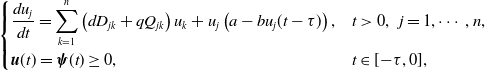
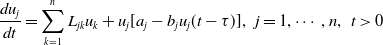 \begin{equation} \displaystyle \frac{du_j}{dt}=\sum _{k=1}^nL_{jk}u_k+u_j[a_j-b_ju_j(t-\tau )],\;\;j=1,\cdots, n, \;\;t\gt 0 \end{equation}
for instance. Here, $u_j$
denotes the population density in patch
$u_j$
denotes the population density in patch $j$
,
$j$
, $(L_{jk})$
is the dispersion matrix,
$(L_{jk})$
is the dispersion matrix, $\tau$
is the time delay and represents the maturation time, and
$\tau$
is the time delay and represents the maturation time, and $a_j$
and
$a_j$
and $b_j$
represent the intrinsic growth rate and intraspecific competition of the species in patch
$b_j$
represent the intrinsic growth rate and intraspecific competition of the species in patch $j$
, respectively. It was shown that time delay can induce Hopf bifurcations for model (1.1) when the dispersion matrix
$j$
, respectively. It was shown that time delay can induce Hopf bifurcations for model (1.1) when the dispersion matrix $(L_{jk})=\epsilon (\hat L_{jk})$
with
$(L_{jk})=\epsilon (\hat L_{jk})$
with $0\lt \epsilon \ll 1$
or
$0\lt \epsilon \ll 1$
or $\epsilon \gg 1$
[Reference Chen, Shen and Wei8, Reference Huang, Chen and Zou24]. Especially, if
$\epsilon \gg 1$
[Reference Chen, Shen and Wei8, Reference Huang, Chen and Zou24]. Especially, if $n=2$
, delay-induced Hopf bifurcations can occur for a wider range of parameters [Reference Liao and Lou31].
$n=2$
, delay-induced Hopf bifurcations can occur for a wider range of parameters [Reference Liao and Lou31].
The species in streams are subject to both random and directed movements. For example, the following Figure 1 represents stream to a lake, and the diffusive flux into and from the lake balances. Therefore, the flux into the lake at the downstream end is only the advective flux, and one can refer to [Reference Lou34, Reference Lou and Lutscher35, Reference Vasilyeva and Lutscher49] for more biological explanation. For the river network illustrated in Figure 1, the dispersion matrix $ (L_{jk})$
in model (1.1) takes the following form:
$ (L_{jk})$
in model (1.1) takes the following form:
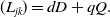 \begin{equation} (L_{jk})=dD+qQ. \end{equation}
Here, $d$
and
$d$
and $q$
are the random diffusion rate and drift rate, respectively; and
$q$
are the random diffusion rate and drift rate, respectively; and $D=(D_{ij})$
and
$D=(D_{ij})$
and $Q=(Q_{ij})$
represent the diffusion pattern and directed movement pattern of individuals, respectively, where
$Q=(Q_{ij})$
represent the diffusion pattern and directed movement pattern of individuals, respectively, where
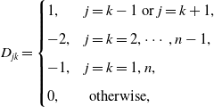 \begin{equation} D_{jk}= \begin{cases} 1, & j=k-1 \text{ or } j=k+1, \\[5pt] -2, & j=k=2,\cdots, n-1, \\[5pt] -1, & j=k=1, n, \\[5pt] 0, & \text{ otherwise, } \end{cases} \end{equation}
and
 \begin{equation} Q_{jk}= \begin{cases} 1, & j=k+1, \\[5pt] -1, & j=k=1,\cdots, n, \\[5pt] 0, & \text{ otherwise. } \end{cases} \end{equation}
The population dynamics in streams have been studied extensively, and it can be modelled by discrete patch models or partial differential equations (PDE) models. It is well known that the stream flow takes individuals to the downstream locations, which is unfavourable for their persistence, see, for example, [Reference Lou and Lutscher35, Reference Lou and Zhou36, Reference Speirs and Gurney45, Reference Vasilyeva and Lutscher49] for PDE models. The directed drift is also a disadvantage for two competing species, and to win the competition, the species need a faster random movement rate to compensate the net loss induced by directed movements, see, for example, [Reference Cantrell, Cosner and Lou3, Reference Chen, Lam and Lou13, Reference Lou and Lutscher35, Reference Lou and Zhou36, Reference Zhou53] for PDE models and, for example, [Reference Chen, Liu and Wu6, Reference Hamida22, Reference Jiang, Lam and Lou25, Reference Jiang, Lam and Lou26, Reference Noble42] for discrete patch models. A natural question is:
-
(Q1) Whether model (1.1) undergoes Hopf bifurcations with $(L_{jk})$
defined in (1.2) and how directed movements of individuals affect Hopf bifurcations?
$(L_{jk})$
defined in (1.2) and how directed movements of individuals affect Hopf bifurcations?

We remark that $d$
and
$d$
and $q$
are normally not proportional, and consequently results in [Reference Chen, Shen and Wei8, Reference Huang, Chen and Zou24] cannot apply to this type of dispersion matrix.
$q$
are normally not proportional, and consequently results in [Reference Chen, Shen and Wei8, Reference Huang, Chen and Zou24] cannot apply to this type of dispersion matrix.

Figure 1. A sample river network.
In this paper, we aim to answer question $(\text{Q}_1)$
and consider the river network illustrated in Figure 1. To emphasise the effect of directed drift, we exclude the effect of spatial heterogeneity, and let
$(\text{Q}_1)$
and consider the river network illustrated in Figure 1. To emphasise the effect of directed drift, we exclude the effect of spatial heterogeneity, and let $a_1=\cdots =a_n=a$
and
$a_1=\cdots =a_n=a$
and $b_1=\cdots =b_n=b$
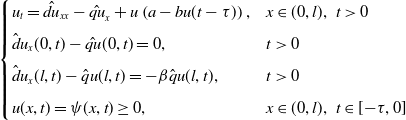
in model (1.1). Then model (1.1) is reduced to the following form:
$b_1=\cdots =b_n=b$
in model (1.1). Then model (1.1) is reduced to the following form:
 \begin{equation} \begin{cases} \displaystyle \frac{d u_j}{d t}=\sum _{k=1}^{n}\left (d D_{jk}+ q Q_{jk}\right )u_k + u_j\left (a- b u_j(t-\tau )\right ),&t\gt 0,\;\;j=1,\cdots, n,\\[9pt] \displaystyle {\boldsymbol{u}}(t)=\boldsymbol{\psi }(t)\geq 0,&t\in [\!-\!\tau, 0], \end{cases} \end{equation}
where $n\geq 2$
is the number of patches,
$n\geq 2$
is the number of patches, $d$
and
$d$
and $q$
are the random diffusion rate and drift rate, respectively,
$q$
are the random diffusion rate and drift rate, respectively, $D=(D_{jk})$
and
$D=(D_{jk})$
and $Q=(Q_{jk})$
are defined in (1.3) and (1.4), respectively, and parameters
$Q=(Q_{jk})$
are defined in (1.3) and (1.4), respectively, and parameters $a,b,\tau \gt 0$
have the same meanings as the above model (1.1).
$a,b,\tau \gt 0$
have the same meanings as the above model (1.1).
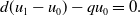
Our study is also motivated by some researches on reaction–diffusion models with time delay. One can refer to [Reference An, Wang and Wang1, Reference Busenberg and Huang2, Reference Chen and Shi9, Reference Chen and Yu12, Reference Guo19, Reference Guo and Yan20, Reference Hu and Yuan23, Reference Su, Wei and Shi46, Reference Yan and Li50, Reference Yan and Li51] and [Reference Chen, Lou and Wei7, Reference Chen, Wei and Zhang11, Reference Jin and Yuan27, Reference Li and Dai30, Reference Liu and Chen33, Reference Ma and Feng38, Reference Meng, Liu and Jin41, Reference Sun and Yuan47] for reaction–diffusion models without and with advection term, respectively. The following reaction–diffusion model with time delay
 \begin{equation} \begin{cases} u_t=\hat{du}_{xx}-\hat{qu}_x + u\left (a- b u(t-\tau )\right ),&x\in (0,l),\;\;t\gt 0\\[5pt] \hat du_x(0,t)-\hat{qu}(0,t)=0,& t\gt 0\\[5pt] \hat du_x(l,t)-\hat q u(l,t)=-\beta \hat q u(l,t),& t\gt 0\\[5pt] u(x,t)=\psi (x,t)\geq 0,&x\in (0,l),\;\;t\in [\!-\!\tau, 0] \end{cases} \end{equation}
models population dynamics in streams, where $\beta \ge 0$
represents the loss of individuals at the downstream end. Actually, model (1.5) can be viewed as a discrete version of model (1.6) with
$\beta \ge 0$
represents the loss of individuals at the downstream end. Actually, model (1.5) can be viewed as a discrete version of model (1.6) with $\beta =1$
, which describes streams into a lake at the downstream end. Divide the interval
$\beta =1$
, which describes streams into a lake at the downstream end. Divide the interval $[0, l]$
into
$[0, l]$
into $n+1$
sub-intervals with equal length
$n+1$
sub-intervals with equal length $\Delta x=l/(n+1)$
, and denote the endpoints by
$\Delta x=l/(n+1)$
, and denote the endpoints by $0, 1,\cdots, n+1$
. Discretising the spatial variable of the first equation of (1.6) at endpoints
$0, 1,\cdots, n+1$
. Discretising the spatial variable of the first equation of (1.6) at endpoints $j=1,\cdots, n$
, we obtain the following equation:
$j=1,\cdots, n$
, we obtain the following equation:
 \begin{equation} \frac{ d u_j}{dt}=\hat{d}\frac{u_{j+1}-2u_j+u_{j-1}}{(\Delta x)^2}-\hat{q}\frac{u_j-u_{j-1}}{\Delta x}+u_j(a-bu_j(t-\tau )), \ \ j=1,\cdots, n, \end{equation}
where $u_j(t)$
is the population density at endpoint
$u_j(t)$
is the population density at endpoint $j$
. Let
$j$
. Let $d=\hat{d}/(\Delta x)^2$
and
$d=\hat{d}/(\Delta x)^2$
and $q=\hat{q}/\Delta x$
. Then we obtain (1.5) from (1.7) for
$q=\hat{q}/\Delta x$
. Then we obtain (1.5) from (1.7) for $j=2,\cdots, n-1$
. At the upstream end, we discretise the no-flux boundary condition and obtain that
$j=2,\cdots, n-1$
. At the upstream end, we discretise the no-flux boundary condition and obtain that
 \begin{equation} d(u_1-u_0)-qu_0=0. \end{equation}
Plugging (1.8) into (1.7) with $j=1$
, we obtain (1.5) for
$j=1$
, we obtain (1.5) for $j=1$
. Similarly, discretising the boundary condition at the downstream end with
$j=1$
. Similarly, discretising the boundary condition at the downstream end with $\beta =1$
, we have
$\beta =1$
, we have $u_{n}=u_{n+1}$
. Plugging it into (1.7), we obtain (1.5) for
$u_{n}=u_{n+1}$
. Plugging it into (1.7), we obtain (1.5) for $j=n$
. The above discretisation for model (1.6) with
$j=n$
. The above discretisation for model (1.6) with $\tau =0$
can be found in [Reference Chen, Shi, Shuai and Wu10, Reference Lou34], and here we include it for the sake of completeness.
$\tau =0$
can be found in [Reference Chen, Shi, Shuai and Wu10, Reference Lou34], and here we include it for the sake of completeness.
For the non-advective case ( $\hat q=0$
), model (1.6) admits a unique positive steady state
$\hat q=0$
), model (1.6) admits a unique positive steady state $u=a/b$
, and it was shown in [Reference Memory40, Reference Yoshida52] that large delay can make such a constant steady state unstable and induce Hopf bifurcations. If
$u=a/b$
, and it was shown in [Reference Memory40, Reference Yoshida52] that large delay can make such a constant steady state unstable and induce Hopf bifurcations. If $\hat d$
and
$\hat d$
and $\hat q$
are proportional with
$\hat q$
are proportional with $\hat q\ne 0$
, delay-induced Hopf bifurcations can also be investigated. Letting
$\hat q\ne 0$
, delay-induced Hopf bifurcations can also be investigated. Letting $\tilde u=e^{-(\hat q/\hat d)x}u$
and
$\tilde u=e^{-(\hat q/\hat d)x}u$
and $\tilde t=dt$
, model (1.6) can be transformed as follows:
$\tilde t=dt$
, model (1.6) can be transformed as follows:
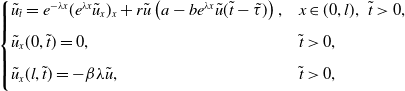 \begin{equation} \begin{cases} \tilde u_{\tilde t}=e^{-\lambda x}(e^{\lambda x}\tilde u_{x})_x+r \tilde u\left (a- be^{\lambda x} \tilde u(\tilde t-\tilde \tau )\right ),&x\in (0,l),\;\;\tilde t\gt 0,\\[5pt] \tilde u_x(0,\tilde t)=0,& \tilde t\gt 0,\\[5pt] \tilde u_x(l,\tilde t)=-\beta \lambda \tilde u,& \tilde t\gt 0,\\[5pt] \end{cases} \end{equation}
where $\lambda =\hat d/\hat q$
,
$\lambda =\hat d/\hat q$
, $r=1/\hat d$
and
$r=1/\hat d$
and $\tilde \tau =\hat d\tau$
. For the case of
$\tilde \tau =\hat d\tau$
. For the case of $\beta =0$
, it was shown in [Reference Chen, Wei and Zhang11] that delay can induce Hopf bifurcations for model (1.9) if
$\beta =0$
, it was shown in [Reference Chen, Wei and Zhang11] that delay can induce Hopf bifurcations for model (1.9) if $r\ll 1$
, which implies that delay-induced Hopf bifurcations can occur if
$r\ll 1$
, which implies that delay-induced Hopf bifurcations can occur if $\hat d$
and
$\hat d$
and $\hat q$
are proportional and both large for the original model (1.6). To our knowledge, the case that
$\hat q$
are proportional and both large for the original model (1.6). To our knowledge, the case that $\hat d$
and
$\hat d$
and $\hat q$
are not proportional is also unknown for model (1.6). Our study on question
$\hat q$
are not proportional is also unknown for model (1.6). Our study on question $(\text{Q}_1)$
also solves this problem in a discrete setting.
$(\text{Q}_1)$
also solves this problem in a discrete setting.
The main results of the paper are summarised as follows. It is well known that large delay can induce Hopf bifurcations for model (1.5) if the directed drift rate $q=0$
(the non-advective case), and the first Hopf bifurcation value is
$q=0$
(the non-advective case), and the first Hopf bifurcation value is $\displaystyle \tau _{non}=\pi /2a$
, which is independent of the random diffusion rate
$\displaystyle \tau _{non}=\pi /2a$
, which is independent of the random diffusion rate $d$
(Proposition 5.1). In contrast, if
$d$
(Proposition 5.1). In contrast, if $q\ne 0$
(the advection case), the first Hopf bifurcation value
$q\ne 0$
(the advection case), the first Hopf bifurcation value $\tau _{adv}$
depends on
$\tau _{adv}$
depends on $d$
and is strictly monotone decreasing in
$d$
and is strictly monotone decreasing in $d\in (\hat d_3,\infty )$
with
$d\in (\hat d_3,\infty )$
with $\hat d_{3}\gg 1$
(Proposition 5.2). Moreover, we show that
$\hat d_{3}\gg 1$
(Proposition 5.2). Moreover, we show that $\tau _{adv}\gt \tau _{non}$
for
$\tau _{adv}\gt \tau _{non}$
for $d\gg 1$
or
$d\gg 1$
or $d\ll 1$
(Propositions 5.2 and 5.3), which suggests that directed movements of the individuals inhibit the occurrence of Hopf bifurcations. The comparison of Hopf bifurcation values between non-advective and advective cases is illustrated in Figure 2. Moreover, we obtain that the total population size is strictly increasing in
$d\ll 1$
(Propositions 5.2 and 5.3), which suggests that directed movements of the individuals inhibit the occurrence of Hopf bifurcations. The comparison of Hopf bifurcation values between non-advective and advective cases is illustrated in Figure 2. Moreover, we obtain that the total population size is strictly increasing in $d\in [\delta, \infty )$
with
$d\in [\delta, \infty )$
with $\delta \gg 1$
(Proposition 2.6 and remark 2.7).
$\delta \gg 1$
(Proposition 2.6 and remark 2.7).
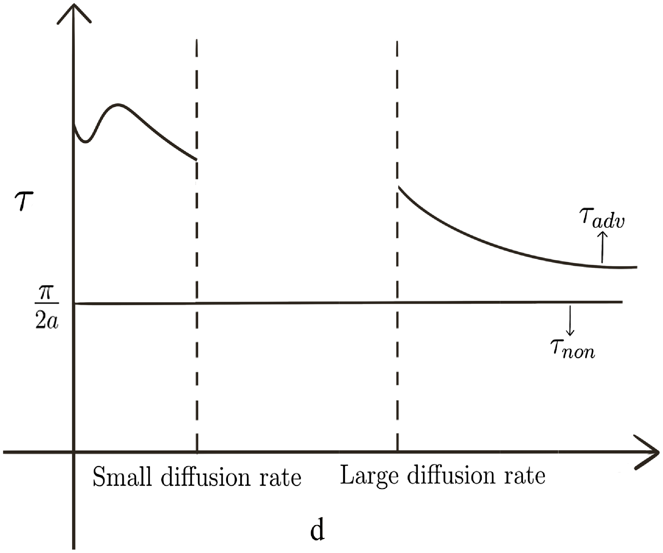
Figure 2. The comparison of Hopf bifurcation values.
For patch models in homogeneous non-advective environments, one can refer to [Reference Fernandes and Aguiar16–Reference Gou, Song and Jin18] for the framework of Turing and Hopf bifurcations, see also [Reference Chang, Duan, Sun and Jin4, Reference Duan, Chang and Jin15] for cross diffusion-induced Turing bifurcations and [Reference Chang, Liu, Sun, Wang and Jin5, Reference Liu, Cong and Su32, Reference Madras, Wu and Zou39, Reference Petit, Asllani, Fanelli, Lauwens and Carletti43, Reference So, Wu and Zou44, Reference Tian and Ruan48] for delay-induced Hopf bifurcations. For homogeneous advective environments, one cannot obtain the explicit expressions for the positive equilibria. This brings some difficulties in bifurcation analysis, and we overcome them by constructing equivalent eigenvalue problems in this paper.
The rest of the paper is organised as follows. In Section 2, we give some preliminaries and obtain some properties for the unique positive equilibrium ${\boldsymbol{u}}_d$
of model (1.5). In Section 3, we study the eigenvalue problem associated with the positive equilibrium
${\boldsymbol{u}}_d$
of model (1.5). In Section 3, we study the eigenvalue problem associated with the positive equilibrium ${\boldsymbol{u}}_d$
for three cases. In Section 4, we obtain the local dynamics and the existence of Hopf bifurcations for model (1.5). Finally, we show the effect of drift rate on Hopf bifurcation values and give some numerical simulations in Section 5.
${\boldsymbol{u}}_d$
for three cases. In Section 4, we obtain the local dynamics and the existence of Hopf bifurcations for model (1.5). Finally, we show the effect of drift rate on Hopf bifurcation values and give some numerical simulations in Section 5.
2. Preliminary
We first list some notations for later use. Denote $\textbf{1}=(1,\cdots, 1)^T$
and define the real and imaginary parts of
$\textbf{1}=(1,\cdots, 1)^T$
and define the real and imaginary parts of $\mu \in \mathbb{C}$
by
$\mu \in \mathbb{C}$
by $\mathcal{R}e \mu$
and
$\mathcal{R}e \mu$
and $\mathcal{I}m \mu$
, respectively. For a space
$\mathcal{I}m \mu$
, respectively. For a space $Z$
, we denote complexification of
$Z$
, we denote complexification of $Z$
to be
$Z$
to be $Z_{\mathbb{C}}\;:\!=\;\{x_1+\mathrm{i}x_2|x_1,x_2\in Z\}$
. For a linear operator
$Z_{\mathbb{C}}\;:\!=\;\{x_1+\mathrm{i}x_2|x_1,x_2\in Z\}$
. For a linear operator $T$
, we define the domain, the range and the kernel of
$T$
, we define the domain, the range and the kernel of $T$
by
$T$
by $\mathscr{D}(T)$
,
$\mathscr{D}(T)$
, $\mathscr{R}(T)$
and
$\mathscr{R}(T)$
and $\mathscr{N}(T)$
, respectively. For
$\mathscr{N}(T)$
, respectively. For $\mathbb{C}^n$
, we choose the inner product
$\mathbb{C}^n$
, we choose the inner product ${\langle {\boldsymbol{u}},{{\boldsymbol{v}}}\rangle }=\sum _{j=1}^{n}\overline{u}_j v_j$
for
${\langle {\boldsymbol{u}},{{\boldsymbol{v}}}\rangle }=\sum _{j=1}^{n}\overline{u}_j v_j$
for ${\boldsymbol{u}},{{\boldsymbol{v}}}\in \mathbb{C}^n$
and denote
${\boldsymbol{u}},{{\boldsymbol{v}}}\in \mathbb{C}^n$
and denote
 \begin{equation*} \begin{split} \|{\boldsymbol{u}}\|_\infty =\max _{j=1,\cdots, n}|u_j|,\ \|{\boldsymbol{u}}\|_2=\left (\sum _{j=1}^{n}|u_j|^2 \right )^{1/2}. \end{split} \end{equation*}
For ${\boldsymbol{u}}=(u_1,\cdots, u_n)^T\in \mathbb{R}^n$
, we write
${\boldsymbol{u}}=(u_1,\cdots, u_n)^T\in \mathbb{R}^n$
, we write ${\boldsymbol{u}}\gg \textbf{0}$
if
${\boldsymbol{u}}\gg \textbf{0}$
if $u_j\gt 0$
for all
$u_j\gt 0$
for all $j=1,\cdots, n$
. For an
$j=1,\cdots, n$
. For an $n\times n$
real-valued matrix
$n\times n$
real-valued matrix $M$
, we denote the spectral bound of
$M$
, we denote the spectral bound of $M$
by:
$M$
by:
 \begin{equation*} \begin{split} s(M)\;:\!=\;\max \{\mathcal{R}e \mu \;:\;\mu \ \text{is an eigenvalue of } M\}, \end{split} \end{equation*}
and the spectral radius of $M$
by:
$M$
by:
 \begin{equation*} \begin{split} \rho (M)\;:\!=\;\max \{|\mu | \;:\;\mu \ \text{is an eigenvalue of } M \}. \end{split} \end{equation*}
An eigenvalue of $M$
with a positive eigenvector is called the principal eigenvalue of
$M$
with a positive eigenvector is called the principal eigenvalue of $M$
. A real-valued square matrix
$M$
. A real-valued square matrix $M$
with non-negative off-diagonal entries is referred to as the essentially non-negative matrix. If
$M$
with non-negative off-diagonal entries is referred to as the essentially non-negative matrix. If $M$
is an irreducible essentially non-negative matrix, then there exists
$M$
is an irreducible essentially non-negative matrix, then there exists $c\gt 0$
such that
$c\gt 0$
such that $M+c I$
is an irreducible non-negative matrix. It follows from [Reference Li and Schneider28, Theorem 2.1] that
$M+c I$
is an irreducible non-negative matrix. It follows from [Reference Li and Schneider28, Theorem 2.1] that
-
(i)
$\rho (M+c I)$
is positive and is an algebraically simple eigenvalue of
$M+cI$
with a positive eigenvector. -
(ii)
$\rho (M+c I)$
is the unique eigenvalue with a non-negative eigenvector.


By (i), we have $s(M)+c=s(M+cI)=\rho (M+cI)$
, and consequently,
$s(M)+c=s(M+cI)=\rho (M+cI)$
, and consequently, $s(M)$
is an algebraically simple eigenvalue of
$s(M)$
is an algebraically simple eigenvalue of $M$
with a positive eigenvector. By (ii), we see that
$M$
with a positive eigenvector. By (ii), we see that $s(M)$
is the unique principal eigenvalue of
$s(M)$
is the unique principal eigenvalue of $M$
.
$M$
.
Consider the following eigenvalue problem:
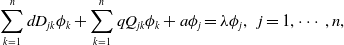 \begin{equation} \sum _{k=1}^{n} d D_{jk} \phi _k+\sum _{k=1}^{n} q Q_{jk}\phi _k + a \phi _j=\lambda \phi _j, \ \ j=1,\cdots, n,\\[5pt] \end{equation}
where $(D_{jk})$
and
$(D_{jk})$
and $(Q_{jk})$
are defined in (1.3) and (1.4), respectively. Since
$(Q_{jk})$
are defined in (1.3) and (1.4), respectively. Since $dD+qQ+aI$
is an irreducible and essentially non-negative matrix, it follows that (2.1) admits a unique principal eigenvalue
$dD+qQ+aI$
is an irreducible and essentially non-negative matrix, it follows that (2.1) admits a unique principal eigenvalue $\lambda _1(d,q)$
with
$\lambda _1(d,q)$
with
 \begin{equation*}\lambda _1(d,q)=s\left (dD+qQ+aI\right ).\end{equation*}
The global dynamics of model (1.5) for $\tau =0$
is determined by the sign of
$\tau =0$
is determined by the sign of $\lambda _1(d,q)$
(see [Reference Cosner14, Reference Li and Shuai29, Reference Lu and Takeuchi37] for the proof).
$\lambda _1(d,q)$
(see [Reference Cosner14, Reference Li and Shuai29, Reference Lu and Takeuchi37] for the proof).
Lemma 2.1.
Suppose that $\tau =0$
. If
$\tau =0$
. If $\lambda _1(d,q)\leq 0$
, then the trivial equilibrium
$\lambda _1(d,q)\leq 0$
, then the trivial equilibrium $\textbf{0}$
of model
(1.5) is globally asymptotically stable; if
$\textbf{0}$
of model
(1.5) is globally asymptotically stable; if $\lambda _1(d,q)\gt 0$
, then model
(1.5) admits a unique positive equilibrium, which is globally asymptotically stable.
$\lambda _1(d,q)\gt 0$
, then model
(1.5) admits a unique positive equilibrium, which is globally asymptotically stable.
For later use, we cite the following result from [Reference Chen, Shi, Shuai and Wu10].
Lemma 2.2.
Let $\lambda _1(d,q)$
be the principal eigenvalue of
(2.1). Then the following statements hold:
$\lambda _1(d,q)$
be the principal eigenvalue of
(2.1). Then the following statements hold:
-
(i) For fixed
$d\gt 0$
,
$\lambda _1(d,q)$
is strictly decreasing with respect to
$q$
in
$[0,\infty )$
, and there exists
$q^*_d\gt 0$
such that
$\lambda _1(d,q^*_d)=0$
,
$\lambda _1(d,q)\lt 0$
for
$q\gt q^*_d$
, and
$\lambda _1(d,q)\gt 0$
for
$q\lt q^*_d$
; -
(ii)
$q^*_d$
is strictly increasing in
$d\in (0,\infty )$
with
$\lim _{d\to 0}q^*_d=a$
and
$\lim _{d\to \infty }q^*_d=na$
.


Here, we remark that Lemma 2.2 (i) follows from [Reference Chen, Shi, Shuai and Wu10, Lemma 3.1 and Proposition 3.2 (i)], and Lemma 2.2 (ii) follows from [Reference Chen, Shi, Shuai and Wu10, Lemma 3.7]. The following result is deduced directly from Lemma 2.2.
Lemma 2.3.
Let $\lambda _1(d,q)$
be the principal eigenvalue of
(2.1). Then the following statements hold:
$\lambda _1(d,q)$
be the principal eigenvalue of
(2.1). Then the following statements hold:
-
(i) If
$q\in (0,a]$
, then
$\lambda _1(d,q)\gt 0$
for all
$d\gt 0$
; -
(ii) If
$q\in (a,na)$
, then there exists
$d^*_q\gt 0$
such that
$\lambda _1(d^*_q,q)=0$
,
$\lambda _1(d,q)\lt 0$
for
$0\lt d\lt d^*_q$
and
$\lambda _1(d,q)\gt 0$
for
$d\gt d^*_q$
; -
(iii) If
$q\in [na,\infty )$
, then
$\lambda _1(d,q)\lt 0$
for all
$d\gt 0$
.


By Lemmas 2.1 and 2.3, we obtain the global dynamics of model (1.5) for $\tau =0$
.
$\tau =0$
.
Proposition 2.4.
Suppose that $d,q,a,b\gt 0$
and
$d,q,a,b\gt 0$
and $\tau =0$
. Then the following statements hold:
$\tau =0$
. Then the following statements hold:
-
(i) If
$q\in (0,a]$
, then model
(1.5) admits a unique positive equilibrium
${\boldsymbol{u}}_{d}\gg \textbf{0}$
for all
$d\gt 0$
, which is globally asymptotically stable;
-
(ii) If
$q\in (a,na)$
, then the trivial equilibrium
$\textbf{0}$
of model
(1.5) is globally asymptotically stable for
$d\in (0,d_q^*]$
; and for
$d\in (d_q^*,\infty )$
, model
(1.5) admits a unique positive equilibrium
${\boldsymbol{u}}_{d}\gg \textbf{0}$
, which is globally asymptotically stable;
-
(iii) If
$q\in [na,\infty )$
, then the trivial equilibrium
$\textbf{0}$
of model
(1.5) is globally asymptotically stable.


Clearly, ${\boldsymbol{u}}_d$
satisfies
${\boldsymbol{u}}_d$
satisfies
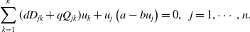 \begin{equation} \displaystyle \sum _{k=1}^{n} (dD_{jk} + q Q_{jk})u_k+u_j\left (a- b u_j\right )=0,\ \ j=1,\cdots, n.\\[5pt] \end{equation}
For simplicity, we first list some notations. Define
 \begin{equation} \mathcal L=(\mathcal L_{jk})\;:\!=\;d_q^*D+qQ+aI, \end{equation}
where $d_q^*$
is defined in Lemma 2.3. It follow from Lemma 2.3 (ii) that
$d_q^*$
is defined in Lemma 2.3. It follow from Lemma 2.3 (ii) that $0$
is the principal eigenvalue of
$0$
is the principal eigenvalue of $\mathcal L$
and a corresponding eigenvector is
$\mathcal L$
and a corresponding eigenvector is
 \begin{equation} \boldsymbol{\eta }=(\eta _1,\cdots, \eta _n)^T\gg 0\;\;\text{with}\;\;\sum _{i=1}^n\eta _i=1. \end{equation}
Clearly, $0$
is also the principal eigenvalue of
$0$
is also the principal eigenvalue of $\mathcal L^T$
and a corresponding eigenvector is
$\mathcal L^T$
and a corresponding eigenvector is
 \begin{equation} \hat{\boldsymbol{\eta }}=(\hat \eta _1,\cdots, \hat \eta _n)^T\gg 0\;\;\text{with}\;\;\sum _{i=1}^n\hat \eta _i=1. \end{equation}
Here, we remark that $0$
is an algebraically simple eigenvalue of
$0$
is an algebraically simple eigenvalue of $\mathcal L$
and
$\mathcal L$
and $\mathcal L^T$
, and the corresponding eigenvector is unique up to multiplying by a scalar. Then, we have the following decompositions:
$\mathcal L^T$
, and the corresponding eigenvector is unique up to multiplying by a scalar. Then, we have the following decompositions:
 \begin{equation} \mathbb{R}^{n}=\textrm{span}\{{\boldsymbol{\eta }}\} \oplus{X}_{1}=\textrm{span}\{{\textbf{1}}\} \oplus{X}_{1}, \end{equation}
where
 \begin{equation} \begin{split}{X}_{1}&\;:\!=\;\left \{\left (x_{1}, \cdots, x_{n}\right )^{T} \in \mathbb{R}^{n} \;:\; \sum _{i=1}^{n}{\hat \eta }_{i} x_{i}=0\right \}.\\[5pt] \end{split} \end{equation}
In fact, for any ${{\boldsymbol{y}}}=(y_1,\cdots, y_n)^T\in \mathbb{R}^n$
,
${{\boldsymbol{y}}}=(y_1,\cdots, y_n)^T\in \mathbb{R}^n$
, ${{\boldsymbol{y}}}=c_1\textbf{1}+\boldsymbol{\xi }_1=c_2\boldsymbol{\eta }+\boldsymbol{\xi }_2$
, where
${{\boldsymbol{y}}}=c_1\textbf{1}+\boldsymbol{\xi }_1=c_2\boldsymbol{\eta }+\boldsymbol{\xi }_2$
, where
 \begin{equation*} c_1=\sum _{i=1}^n\hat \eta _iy_i,\;\;\boldsymbol {\xi }_1={{\boldsymbol{y}}}-c_1\textbf{1}\in X_1,\;\;c_2=\displaystyle \frac {\sum _{i=1}^n\hat \eta _iy_i}{\sum _{i=1}^n\eta _i\hat \eta _i},\;\;\boldsymbol {\xi }_2={{\boldsymbol{y}}}-c_2\boldsymbol {\eta }\in X_1.\\[5pt] \end{equation*}
Now, we explore further properties on the positive equilibrium ${\boldsymbol{u}}_d$
.
${\boldsymbol{u}}_d$
.
Proposition 2.5.
Let $\boldsymbol{\eta }$
,
$\boldsymbol{\eta }$
, $\hat{\boldsymbol{\eta }}$
and
$\hat{\boldsymbol{\eta }}$
and $X_1$
be defined in
(2.4),
(2.5) and
(2.7), respectively. Then the following statements hold:
$X_1$
be defined in
(2.4),
(2.5) and
(2.7), respectively. Then the following statements hold:
-
(i) For fixed
$q\in (0,a)$
,
${\boldsymbol{u}}_{d}$
is continuously differentiable with respect to
$d\in [0,\infty )$
, where
${\boldsymbol{u}}_d={\boldsymbol{u}}_{0}$
for
$d=0$
, and
${\boldsymbol{u}}_{0}$
is the unique solution of
(2.8)Moreover,
\begin{equation} \begin{cases} u_{0,1}=\displaystyle \frac{a-q}{b},\;\;qu_{0,j-1}=-u_{0,j}\left (a-q-bu_{0,j}\right )\;\;\text{for}\;\;j=2,\cdots, n,\\[5pt] u_{0,j}\gt 0\;\;\text{for}\;\;j=1,\cdots, n. \end{cases} \end{equation}
(2.9)
\begin{equation} u_{0,1}\lt \dots \lt u_{0,n} ; \end{equation}
-
(ii) For fixed
$q\in (a,na)$
,
${\boldsymbol{u}}_d$
can be represented as follows:
(2.10)Here,
\begin{equation} {\boldsymbol{u}}_d=(d-d_q^*)(\alpha _d\boldsymbol{\eta }+\boldsymbol{\xi }_d)\;\;\text{for}\;\;d\gt d^*_q. \end{equation}
$(\alpha _d,\boldsymbol{\xi }_d)\in \mathbb{R}\times X_1$
is continuously differentiable with respect to
$d\in [d^*_q,\infty )$
, and for
$d=d^*_q$
,
$(\alpha _d,\boldsymbol{\xi }_d)=\left (\alpha ^*,\textbf{0}\right )$
with
(2.11)
\begin{equation} \alpha ^*=\frac{\sum _{j,k=1}^nD_{jk}\eta _k\hat \eta _j}{b\sum _{j=1}^n\eta _j^2\hat \eta _j}\gt 0. \end{equation}


Proof. (i) It follows from Proposition 2.4 that ${\boldsymbol{u}}_d$
is the unique positive equilibrium of (1.5), which is stable (non-degenerate). Therefore, by the implicit function theorem, we obtain that
${\boldsymbol{u}}_d$
is the unique positive equilibrium of (1.5), which is stable (non-degenerate). Therefore, by the implicit function theorem, we obtain that ${\boldsymbol{u}}_d$
is continuously differentiable for
${\boldsymbol{u}}_d$
is continuously differentiable for $d\in (0,\infty )$
. Then we need to show that
$d\in (0,\infty )$
. Then we need to show that ${\boldsymbol{u}}_d$
is continuously differentiable for
${\boldsymbol{u}}_d$
is continuously differentiable for $d\in [0,d_1]$
with
$d\in [0,d_1]$
with $0\lt d_1\ll 1$
.
$0\lt d_1\ll 1$
.
Define
 \begin{eqnarray*}{{\boldsymbol{H}}}(d,{\boldsymbol{u}})= \begin{pmatrix} \displaystyle d\sum _{k=1}^{n} D_{1k} u_k-qu_{1}+u_{1}\left (a-bu_{1}\right ) \\[5pt] \displaystyle d\sum _{k=1}^{n} D_{2k} u_k+q\left (u_{1}-u_{2}\right )+u_{2}\left (a-bu_{2}\right ) \\[5pt] \displaystyle \vdots \\[5pt] \displaystyle d\sum _{k=1}^{n} D_{nk} u_k+q\left (u_{n-1}-u_{n}\right )+u_{n}\left (a-bu_{n}\right ) \end{pmatrix}. \end{eqnarray*}
Clearly, ${{\boldsymbol{H}}}(0,{\boldsymbol{u}}_0)=\textbf{0}$
, where
${{\boldsymbol{H}}}(0,{\boldsymbol{u}}_0)=\textbf{0}$
, where ${\boldsymbol{u}}_{0}$
is defined by (2.8). Let
${\boldsymbol{u}}_{0}$
is defined by (2.8). Let $D_{{\boldsymbol{u}}}{{\boldsymbol{H}}}(0,{\boldsymbol{u}}_0)$
be the Jacobian matrix of
$D_{{\boldsymbol{u}}}{{\boldsymbol{H}}}(0,{\boldsymbol{u}}_0)$
be the Jacobian matrix of ${{\boldsymbol{H}}}(d,{\boldsymbol{u}})$
with respect to
${{\boldsymbol{H}}}(d,{\boldsymbol{u}})$
with respect to ${\boldsymbol{u}}$
at
${\boldsymbol{u}}$
at $(0,{\boldsymbol{u}}_0)$
. A direct computation implies that
$(0,{\boldsymbol{u}}_0)$
. A direct computation implies that $D_{{\boldsymbol{u}}}{{\boldsymbol{H}}}(0,{\boldsymbol{u}}_0)=(h_{j,k})$
with
$D_{{\boldsymbol{u}}}{{\boldsymbol{H}}}(0,{\boldsymbol{u}}_0)=(h_{j,k})$
with
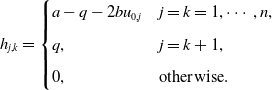 \begin{eqnarray*} h_{j,k}= \begin{cases} a-q-2bu_{0,j} & j=k=1,\cdots, n,\\[5pt] q, &j=k+1,\\[5pt] 0, &\text{otherwise}. \end{cases} \end{eqnarray*}
By (2.8), we have $\displaystyle \frac{a-q}{b}=u_{0,1}\lt \dots \lt u_{0,n}$
, which implies that
$\displaystyle \frac{a-q}{b}=u_{0,1}\lt \dots \lt u_{0,n}$
, which implies that $D_{{\boldsymbol{u}}}{{\boldsymbol{H}}}(0,{\boldsymbol{u}}_0)$
is invertible. Then we see from the implicit function theorem that there exist
$D_{{\boldsymbol{u}}}{{\boldsymbol{H}}}(0,{\boldsymbol{u}}_0)$
is invertible. Then we see from the implicit function theorem that there exist $d_{1}\gt 0$
, and a continuously differentiable mapping
$d_{1}\gt 0$
, and a continuously differentiable mapping
 \begin{equation*}d \in [0,d_{1}]\mapsto {\boldsymbol{u}}(d) =\left (u_{1}(d),\cdots, u_{n}(d)\right )^{T} \in \mathbb {R}^n\end{equation*}
such that ${{\boldsymbol{H}}}(d,{\boldsymbol{u}}(d))=0$
,
${{\boldsymbol{H}}}(d,{\boldsymbol{u}}(d))=0$
, ${\boldsymbol{u}}(d)\gg \textbf{0}$
, and
${\boldsymbol{u}}(d)\gg \textbf{0}$
, and ${\boldsymbol{u}}(0)={\boldsymbol{u}}_0$
. Therefore,
${\boldsymbol{u}}(0)={\boldsymbol{u}}_0$
. Therefore, ${\boldsymbol{u}}(d)$
is the positive equilibrium of model (1.5) for small
${\boldsymbol{u}}(d)$
is the positive equilibrium of model (1.5) for small $d$
. This combined with Proposition 2.4 implies that
$d$
. This combined with Proposition 2.4 implies that ${\boldsymbol{u}}(d)= {\boldsymbol{u}}_{d}$
. Consequently,
${\boldsymbol{u}}(d)= {\boldsymbol{u}}_{d}$
. Consequently, ${\boldsymbol{u}}_{d}$
is continuously differentiable for
${\boldsymbol{u}}_{d}$
is continuously differentiable for $d \in [0,\infty )$
.
$d \in [0,\infty )$
.
(ii) Using similar arguments as in (i), we see that ${\boldsymbol{u}}_d$
is continuously differentiable for
${\boldsymbol{u}}_d$
is continuously differentiable for $d\in (d_q^*,\infty )$
. By the first decomposition in (2.6), we see that
$d\in (d_q^*,\infty )$
. By the first decomposition in (2.6), we see that ${\boldsymbol{u}}_d$
can be represented as in (2.10), where
${\boldsymbol{u}}_d$
can be represented as in (2.10), where $\alpha _d$
and
$\alpha _d$
and $\boldsymbol{\xi }_d$
are also continuously differentiable for
$\boldsymbol{\xi }_d$
are also continuously differentiable for $d\in (d_q^*,\infty )$
. Then we need to show that
$d\in (d_q^*,\infty )$
. Then we need to show that $\alpha _d$
and
$\alpha _d$
and $\boldsymbol{\xi }_d$
are also continuously differentiable for
$\boldsymbol{\xi }_d$
are also continuously differentiable for $d\in [d_q^*,\tilde d_1)$
with
$d\in [d_q^*,\tilde d_1)$
with $0\lt \tilde d_1-d_q^*\ll 1$
.
$0\lt \tilde d_1-d_q^*\ll 1$
.
We first show that $ \alpha ^*\gt 0$
. A direct computation yields
$ \alpha ^*\gt 0$
. A direct computation yields
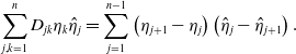 \begin{equation} \sum _{j,k=1}^nD_{jk}\eta _k\hat \eta _j =\sum _{j=1}^{n-1}\left (\eta _{j+1}-\eta _j\right )\left (\hat{\eta }_j-\hat{\eta }_{j+1}\right ). \end{equation}
Noticing that $\boldsymbol{\eta }$
(respectively,
$\boldsymbol{\eta }$
(respectively, $\hat{\boldsymbol{\eta }}$
) is an eigenvector of
$\hat{\boldsymbol{\eta }}$
) is an eigenvector of $\mathcal L$
(respectively,
$\mathcal L$
(respectively, $\mathcal L^T$
) corresponding to eigenvalue
$\mathcal L^T$
) corresponding to eigenvalue $0$
, we have
$0$
, we have
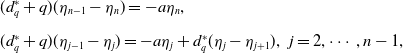 \begin{equation*} \begin{split} &(d^*_q+q)(\eta _{n-1}-\eta _n)=-a \eta _n,\\[5pt] &(d^*_q+q)(\eta _{j-1}-\eta _j)=-a\eta _j+d^*_q(\eta _{j}-\eta _{j+1}),\;\;j=2,\cdots, n-1, \end{split} \end{equation*}
and
 \begin{equation*} \begin{split} &(d^*_q+q)(\hat{\eta }_{2}-\hat{\eta }_1)=-a\hat{\eta }_1,\\[5pt] &(d^*_q+q)(\hat{\eta }_{j+1}-\hat{\eta }_{j})=-a\eta _j+d^*_q(\hat{\eta }_{j}-\hat{\eta }_{j-1}),\;\;j=2,\cdots, n-1, \end{split} \end{equation*}
which implies that $\eta _1\lt \eta _2\lt \dots \lt \eta _n$
and
$\eta _1\lt \eta _2\lt \dots \lt \eta _n$
and $\hat{\eta }_1\gt \hat{\eta }_2\gt \dots \gt \hat{\eta }_n$
. This combined with (2.11) and (2.12) yields
$\hat{\eta }_1\gt \hat{\eta }_2\gt \dots \gt \hat{\eta }_n$
. This combined with (2.11) and (2.12) yields $\alpha ^*\gt 0$
.
$\alpha ^*\gt 0$
.
By the definition of $\mathcal L$
, we rewrite (2.2) as follows:
$\mathcal L$
, we rewrite (2.2) as follows:
 \begin{equation} \sum _{k=1}^n \mathcal L_{jk}u_k+(d-d^*_q)\sum _{j=1}^nD_{jk}u_k-bu_j^2=0. \end{equation}
From the first decomposition in (2.6), we see that ${\boldsymbol{u}}$
in (2.13) can be represented as follows:
${\boldsymbol{u}}$
in (2.13) can be represented as follows:
 \begin{equation} {\boldsymbol{u}}=(d-d^*_q)(\alpha \boldsymbol{\eta } +\boldsymbol{\xi })\;\; \text{for}\;\;d\gt d_q^*. \end{equation}
Plugging (2.14) into (2.13), we have
 \begin{equation} \sum _{k=1}^n \mathcal L_{jk}\xi _{k}+(d-d^*_q)\left [\sum _{j=1}^nD_{jk}(\alpha \eta _k+\xi _{k})-b(\alpha \eta _j+\xi _{j})^2\right ]=0,\;\;\;\;j=1,\cdots, n. \end{equation}
Denoting the left side of (2.15) by $y_j$
, we see from the second decomposition in (2.6) that
$y_j$
, we see from the second decomposition in (2.6) that
 \begin{equation*} \begin{split} &{{\boldsymbol{y}}}=(y_1,\cdots, y_n)^T=c\textbf{1}+{{\boldsymbol{z}}}\;\;\text{with}\;\; c=\sum _{j=1}^n\hat \eta _jy_j\;\;\text{and}\;\;{{\boldsymbol{z}}}\in X_1.\\[5pt] \end{split} \end{equation*}
Therefore, ${{\boldsymbol{y}}}=\textbf{0}$
if and only if
${{\boldsymbol{y}}}=\textbf{0}$
if and only if $c=0$
and
$c=0$
and ${{\boldsymbol{z}}}=\textbf{0}$
. Since
${{\boldsymbol{z}}}=\textbf{0}$
. Since $\mathcal L\boldsymbol{\xi }\in X_1$
, it follows that
$\mathcal L\boldsymbol{\xi }\in X_1$
, it follows that
 \begin{equation*} c=(d-d_q^*)G_2\;\;\text {and}\;\;{{\boldsymbol{z}}}=\left (G_{1,1},\cdots, G_{1,n}\right )^T, \end{equation*}
where
 \begin{equation*} \begin{split} &G_{1,j}(d,\alpha, \boldsymbol{\xi })=\sum _{k=1}^n \mathcal L_{jk}\xi _{k}+(d-d^*_q)\left [\sum _{j=1}^nD_{jk}(\alpha \eta _k+\xi _{k})-b(\alpha \eta _j+\xi _{j})^2\right ]\\[5pt] &-(d-d^*_q)G_2(d,\alpha, \boldsymbol{\xi }),\;\;\;\;j=1,\cdots, n,\\[5pt] &G_2(d,\alpha, \boldsymbol{\xi })=\sum _{j=1}^n\hat \eta _j\left [\sum _{k=1}^nD_{jk}(\alpha \eta _k+\xi _k)-b(\alpha \eta _j+\xi _j)^2\right ]. \end{split} \end{equation*}
Define ${{\boldsymbol{G}}}(d,\alpha, \boldsymbol{\xi }) \;:\; \mathbb{R}^2\times X_1\to X_1\times \mathbb{R}$
by
${{\boldsymbol{G}}}(d,\alpha, \boldsymbol{\xi }) \;:\; \mathbb{R}^2\times X_1\to X_1\times \mathbb{R}$
by ${{\boldsymbol{G}}}\;:\!=\;(G_{1,1},\cdots, G_{1,n},G_2)^T$
. It follows that, for
${{\boldsymbol{G}}}\;:\!=\;(G_{1,1},\cdots, G_{1,n},G_2)^T$
. It follows that, for $d\gt d_q^*$
,
$d\gt d_q^*$
, ${\boldsymbol{u}}$
(represented in (2.14)) is a solution of (2.13) if and only if
${\boldsymbol{u}}$
(represented in (2.14)) is a solution of (2.13) if and only if $(\alpha, \boldsymbol{\xi })\in \mathbb{R}\times X_1$
is a solution of
$(\alpha, \boldsymbol{\xi })\in \mathbb{R}\times X_1$
is a solution of ${{\boldsymbol{G}}}(d,\alpha, \boldsymbol{\xi })=\textbf{0}$
.
${{\boldsymbol{G}}}(d,\alpha, \boldsymbol{\xi })=\textbf{0}$
.
Now we consider the equivalent problem ${{\boldsymbol{G}}}(d,\alpha, \boldsymbol{\xi })=\textbf{0}$
. Clearly,
${{\boldsymbol{G}}}(d,\alpha, \boldsymbol{\xi })=\textbf{0}$
. Clearly, ${{\boldsymbol{G}}}(d_q^*,\alpha ^*,\textbf{0})=\textbf{0}$
. Let
${{\boldsymbol{G}}}(d_q^*,\alpha ^*,\textbf{0})=\textbf{0}$
. Let ${{\boldsymbol{T}}}\left (\check{\alpha },\check{\boldsymbol{\xi }}\right )=(T_{1,1}, \cdots, T_{1,n},T_2)^T \;:\; \mathbb{R}\times X_1 \mapsto X_1\times \mathbb{R}$
be the Fréchet derivative of
${{\boldsymbol{T}}}\left (\check{\alpha },\check{\boldsymbol{\xi }}\right )=(T_{1,1}, \cdots, T_{1,n},T_2)^T \;:\; \mathbb{R}\times X_1 \mapsto X_1\times \mathbb{R}$
be the Fréchet derivative of ${\boldsymbol{G}}$
with respect to
${\boldsymbol{G}}$
with respect to $(\alpha, \boldsymbol{\xi })$
at
$(\alpha, \boldsymbol{\xi })$
at $(d^*_q,\alpha ^*,\textbf{0})$
. Then we compute that
$(d^*_q,\alpha ^*,\textbf{0})$
. Then we compute that
 \begin{equation*} \begin{split} T_{1,j}\left (\check{\alpha }, \check{\boldsymbol{\xi }}\right )=&\sum _{k=1}^{n} \mathcal L_{jk} \check{\xi }_{k},\;\;j=1,\cdots, n,\\[5pt] T_{2}\left (\check{\alpha }, \check{\boldsymbol{\xi }}\right )=&\sum _{j=1}^{n}\hat{\eta }_j\left (\sum _{k=1}^{n}D_{jk}\eta _k-2b\alpha ^*\eta ^2_j\right )\check{\alpha }+ \sum _{j=1}^{n}\hat{\eta }_j\left (\sum _{k=1}^{n}D_{jk}\check{\xi }_{k}-2b\alpha ^*\eta _j\check \xi _j\right ).\\[5pt] \end{split} \end{equation*}
By (2.11), we see that ${\boldsymbol{T}}$
is a bijection from
${\boldsymbol{T}}$
is a bijection from $\mathbb{R} \times X_1$
to
$\mathbb{R} \times X_1$
to $X_1\times \mathbb{R}$
. Then it follows from the implicit function theorem that there exists
$X_1\times \mathbb{R}$
. Then it follows from the implicit function theorem that there exists $\tilde{d}_1\gt d^*_q$
and a continuously differentiable mapping
$\tilde{d}_1\gt d^*_q$
and a continuously differentiable mapping $d\in \left [d^*_q,\tilde{d}_1\right ] \mapsto \left (\tilde{\alpha }_d, \tilde{\boldsymbol{\xi }}_d\right )\in \mathbb{R}\times X_1$
such that
$d\in \left [d^*_q,\tilde{d}_1\right ] \mapsto \left (\tilde{\alpha }_d, \tilde{\boldsymbol{\xi }}_d\right )\in \mathbb{R}\times X_1$
such that ${{\boldsymbol{G}}}(d,\tilde{\alpha }_d,\tilde{\boldsymbol{\xi }}_d)=\textbf{0}$
, and
${{\boldsymbol{G}}}(d,\tilde{\alpha }_d,\tilde{\boldsymbol{\xi }}_d)=\textbf{0}$
, and $\tilde{\alpha }_d=\alpha ^*$
and
$\tilde{\alpha }_d=\alpha ^*$
and $\tilde{\boldsymbol{\xi }}_d=\textbf{0}$
for
$\tilde{\boldsymbol{\xi }}_d=\textbf{0}$
for $d=d^*_q$
. It follows from Proposition 2.4 and Eq. (2.6) that the unique positive equilibrium
$d=d^*_q$
. It follows from Proposition 2.4 and Eq. (2.6) that the unique positive equilibrium ${\boldsymbol{u}}_d$
can be represented as (2.10) for
${\boldsymbol{u}}_d$
can be represented as (2.10) for $d\gt d_q^*$
. Then we obtain that
$d\gt d_q^*$
. Then we obtain that $\alpha _d=\tilde{\alpha }_d$
,
$\alpha _d=\tilde{\alpha }_d$
, ${\boldsymbol{\xi }}_d=\tilde{\boldsymbol{\xi }}_d$
for
${\boldsymbol{\xi }}_d=\tilde{\boldsymbol{\xi }}_d$
for $d\in \left (d^*_q,\tilde{d}_1\right ]$
. Therefore,
$d\in \left (d^*_q,\tilde{d}_1\right ]$
. Therefore, $\alpha _d$
and
$\alpha _d$
and ${\boldsymbol{\xi }}_d$
are continuously differentiable for
${\boldsymbol{\xi }}_d$
are continuously differentiable for $d\in \left [d^*_q,\infty \right )$
if we define
$d\in \left [d^*_q,\infty \right )$
if we define $(\alpha _d,\boldsymbol{\xi }_d)=\left (\alpha ^*,\textbf{0}\right )$
for
$(\alpha _d,\boldsymbol{\xi }_d)=\left (\alpha ^*,\textbf{0}\right )$
for $d=d^*_q$
.
$d=d^*_q$
.
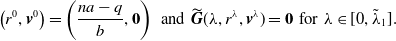
Now, we consider the case $d\gg 1$
. Clearly,
$d\gg 1$
. Clearly, ${\boldsymbol{u}}_d$
satisfies
${\boldsymbol{u}}_d$
satisfies
 \begin{equation} \displaystyle \ \sum _{k=1}^{n} D_{jk} u_k+ \lambda \left [q\sum _{k=1}^{n} Q_{jk}u_k+u_j\left (a- b u_j\right )\right ]=0,\;\;j=1,\cdots, n\\[5pt] \end{equation}
with $d=1/\lambda$
. To avoid confusion, we denote
$d=1/\lambda$
. To avoid confusion, we denote ${\boldsymbol{u}}_d$
by
${\boldsymbol{u}}_d$
by ${\boldsymbol{u}}^\lambda$
for the case
${\boldsymbol{u}}^\lambda$
for the case $d\gg 1$
. Then the properties of
$d\gg 1$
. Then the properties of ${\boldsymbol{u}}_d$
for
${\boldsymbol{u}}_d$
for $d\gg 1$
is equivalent to
$d\gg 1$
is equivalent to ${\boldsymbol{u}}^\lambda$
for
${\boldsymbol{u}}^\lambda$
for $0\lt \lambda \ll 1$
. Clearly,
$0\lt \lambda \ll 1$
. Clearly, $s(D)=0$
is the principal eigenvalue of
$s(D)=0$
is the principal eigenvalue of $D$
, and a corresponding eigenvector is
$D$
, and a corresponding eigenvector is
 \begin{equation} \begin{split} \boldsymbol{\varsigma }=(\varsigma _1,\cdots, \varsigma _n)^T \;\;\text{with} \;\;\varsigma _j=\frac{1}{n}\;\;\text{for all} \; \;j=1,\cdots, n. \end{split} \end{equation}
Define
 \begin{equation} \begin{split} \displaystyle \widetilde{X}_1=\left \{(x_1,\cdots, x_n)^T \in \mathbb{R}^n\;:\;\sum _{j=1}^{n}x_j=0\right \}, \end{split} \end{equation}
and $\mathbb{R}^n$
also has the following decomposition:
$\mathbb{R}^n$
also has the following decomposition:
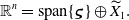 \begin{equation} \mathbb{R}^n=\text{span}\{\boldsymbol{\varsigma }\}\oplus \widetilde{X}_1. \end{equation}
Proposition 2.6.
Suppose that $q\in (0,na)$
, let
$q\in (0,na)$
, let ${\boldsymbol{u}}^\lambda$
be the unique positive solution of
(2.16), and define
${\boldsymbol{u}}^\lambda$
be the unique positive solution of
(2.16), and define ${\boldsymbol{u}}^0=(u^{0}_1,\cdots, u^{0}_1)^T$
, where
${\boldsymbol{u}}^0=(u^{0}_1,\cdots, u^{0}_1)^T$
, where
 \begin{equation*}\displaystyle u^0_{j}=\frac {na-q}{nb} \;\;\text {for all}\;\; j=1,\cdots, n.\end{equation*}
Then the following statements hold:
-
(i)
${\boldsymbol{u}}^{\lambda }=\left (u^\lambda _1,u^\lambda _2,\cdots, u^\lambda _n\right )$
is continuously differentiable for
$\lambda \in [0,\lambda _q^*)$
; -
(ii)
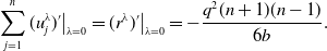
(2.20)
\begin{equation} \sum _{j=1}^{n}\left (u^{\lambda }_j\right )'\big |_{\lambda =0}=-\frac{q^2(n+1)(n-1)}{6b}\lt 0, \end{equation}
and the total population size
$\sum _{j=1}^n u^{\lambda }_j$
is strictly decreasing in
$\lambda \in (0,\epsilon )$
with
$\epsilon \ll 1$
.


Here, $'$
is the derivative with respect to
$'$
is the derivative with respect to $\lambda$
and
$\lambda$
and
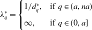 \begin{equation*} \lambda _q^*=\begin{cases} 1/d_q^*,&\text{if}\;\; q\in (a,na)\\[5pt] \infty, &\text{if}\;\; q\in (0,a] \end{cases} \end{equation*}
with $d_q^*$
defined in Proposition 2.5
.
$d_q^*$
defined in Proposition 2.5
.
Proof. (i) By Proposition 2.5, we see that ${\boldsymbol{u}}^{\lambda }$
is continuously differentiable for
${\boldsymbol{u}}^{\lambda }$
is continuously differentiable for $\lambda \in (0,\lambda _q^*)$
. Then we need to show that
$\lambda \in (0,\lambda _q^*)$
. Then we need to show that ${\boldsymbol{u}}^{\lambda }$
is continuously differentiable for
${\boldsymbol{u}}^{\lambda }$
is continuously differentiable for $\lambda \in [0,\tilde \lambda _1)$
with
$\lambda \in [0,\tilde \lambda _1)$
with $0\lt \tilde \lambda _1\ll 1$
. From the decomposition in (2.19), we see that
$0\lt \tilde \lambda _1\ll 1$
. From the decomposition in (2.19), we see that ${\boldsymbol{u}}=(u_1,\cdots, u_n)^T$
in (2.16) can be represented as follows:
${\boldsymbol{u}}=(u_1,\cdots, u_n)^T$
in (2.16) can be represented as follows:
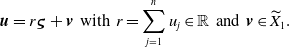 \begin{equation} {\boldsymbol{u}}=r\boldsymbol{\varsigma } +{{{\boldsymbol{v}}}}\;\;\text{with}\;\; r=\sum _{j=1}^nu_j\in \mathbb{R}\;\;\text{and}\;\;{{\boldsymbol{v}}}\in \widetilde{X}_1. \end{equation}
Plugging (2.21) into (2.16), we have
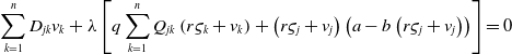 \begin{equation} \displaystyle \sum _{k=1}^{n} D_{jk} v_k+ \lambda \left [q\sum _{k=1}^{n} Q_{jk}\left (r \varsigma _k + v_k\right )+\left (r \varsigma _j + v_j\right )\left (a- b \left (r\varsigma _j + v_j\right )\right )\right ]=0 \end{equation}
for $j=1,\cdots, n$
. Denoting the left side of (2.22) by
$j=1,\cdots, n$
. Denoting the left side of (2.22) by $\widetilde y_j$
, we see from (2.19) that
$\widetilde y_j$
, we see from (2.19) that
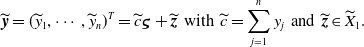 \begin{equation*} \begin{split} &\widetilde{{{\boldsymbol{y}}}}=(\widetilde y_1,\cdots, \widetilde y_n)^T=\widetilde c\boldsymbol{\varsigma }+\widetilde{{{\boldsymbol{z}}}}\;\;\text{with}\;\; \widetilde{c}=\sum _{j=1}^ny_j\;\;\text{and}\;\;\widetilde{{{\boldsymbol{z}}}}\in \widetilde{X}_1.\\[5pt] \end{split} \end{equation*}
Therefore, $\widetilde{{{\boldsymbol{y}}}}=\textbf{0}$
if and only if
$\widetilde{{{\boldsymbol{y}}}}=\textbf{0}$
if and only if $\widetilde c=0$
and
$\widetilde c=0$
and $\widetilde{{{\boldsymbol{z}}}}=\textbf{0}$
. This combined with (2.22) implies that
$\widetilde{{{\boldsymbol{z}}}}=\textbf{0}$
. This combined with (2.22) implies that
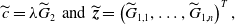 \begin{equation*} \widetilde c=\lambda \widetilde {G}_2\;\;\text {and}\;\;\widetilde {{{\boldsymbol{z}}}}=\left (\widetilde {G}_{1,1},\dots, \widetilde {G}_{1,n}\right )^T, \end{equation*}
where
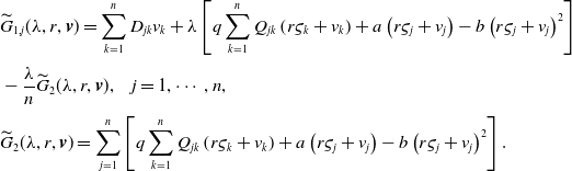 \begin{equation*} \begin{split} &\widetilde{G}_{1,j}(\lambda, r,{{\boldsymbol{v}}})=\sum _{k=1}^n D_{jk}v_{k}+ \lambda \left [q\sum _{k=1}^{n} Q_{jk}\left (r\varsigma _k + v_k\right )+a\left (r \varsigma _j +v_j\right )- b \left (r\varsigma _j + v_j\right )^2\right ]\\[3pt] &-\frac{\lambda }{n}\widetilde{G}_2(\lambda, r,{{\boldsymbol{v}}}),\;\;\;\;j=1,\cdots, n,\\[3pt] &\widetilde{G}_2(\lambda, r,{{\boldsymbol{v}}})=\sum _{j=1}^n\left [q\sum _{k=1}^{n} Q_{jk}\left (r\varsigma _k + v_k\right )+a\left (r\varsigma _j + v_j\right )- b \left (r\varsigma _j + v_j\right )^2\right ]. \end{split} \end{equation*}
Define $ \widetilde{{{\boldsymbol{G}}}}(\lambda, r,{{\boldsymbol{v}}}) \;:\; \mathbb{R}^2\times \widetilde{X}_1\to \widetilde{X}_1\times \mathbb{R}$
by
$ \widetilde{{{\boldsymbol{G}}}}(\lambda, r,{{\boldsymbol{v}}}) \;:\; \mathbb{R}^2\times \widetilde{X}_1\to \widetilde{X}_1\times \mathbb{R}$
by $ \widetilde{{{\boldsymbol{G}}}}\;:\!=\;(\widetilde{G}_{1,1},\cdots, \widetilde{G}_{1,n},G_2)^T$
. It follows that, for
$ \widetilde{{{\boldsymbol{G}}}}\;:\!=\;(\widetilde{G}_{1,1},\cdots, \widetilde{G}_{1,n},G_2)^T$
. It follows that, for $\lambda \in [0,\lambda _q^*)$
,
$\lambda \in [0,\lambda _q^*)$
, ${\boldsymbol{u}}$
(represented in (2.21)) is a solution of (2.16) if and only if
${\boldsymbol{u}}$
(represented in (2.21)) is a solution of (2.16) if and only if $(r,{{\boldsymbol{v}}})\in \mathbb{R}\times \widetilde{X}_1$
is a solution of
$(r,{{\boldsymbol{v}}})\in \mathbb{R}\times \widetilde{X}_1$
is a solution of $\widetilde{{{\boldsymbol{G}}}}(\lambda, r,{{\boldsymbol{v}}})=\textbf{0}$
. Then using similar arguments as in the proof of Proposition 2.5, we can show that there exists
$\widetilde{{{\boldsymbol{G}}}}(\lambda, r,{{\boldsymbol{v}}})=\textbf{0}$
. Then using similar arguments as in the proof of Proposition 2.5, we can show that there exists $\tilde{\lambda }_1\gt 0$
and a continuously differentiable mapping
$\tilde{\lambda }_1\gt 0$
and a continuously differentiable mapping $\lambda \in \left [0,\tilde{\lambda }_1\right ] \mapsto \left (r^\lambda, {{\boldsymbol{v}}}^\lambda \right )\in \mathbb{R}\times \widetilde X_1$
such that
$\lambda \in \left [0,\tilde{\lambda }_1\right ] \mapsto \left (r^\lambda, {{\boldsymbol{v}}}^\lambda \right )\in \mathbb{R}\times \widetilde X_1$
such that
 \begin{equation} \left (r^0,{{\boldsymbol{v}}}^0\right )=\left (\frac{na-q}{b},\textbf{0}\right )\;\;\text{and}\;\;\widetilde{{{\boldsymbol{G}}}}(\lambda, r^\lambda, {{\boldsymbol{v}}}^\lambda )=\textbf{0}\;\;\text{for}\;\;\lambda \in [0,\tilde{\lambda }_1]. \end{equation}
This combined with (2.21) implies that, for $\lambda \in (0,\tilde \lambda _1)$
,
$\lambda \in (0,\tilde \lambda _1)$
,
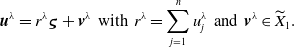 \begin{equation} {\boldsymbol{u}}^\lambda =r^\lambda \boldsymbol \varsigma +{{\boldsymbol{v}}}^\lambda \;\;\text{with}\;\;r^\lambda =\sum _{j=1}^n u_j^\lambda \;\;\text{and}\;\;{{\boldsymbol{v}}}^\lambda \in \widetilde{X}_1. \end{equation}
Therefore, ${\boldsymbol{u}}^{\lambda }$
is continuously differentiable for
${\boldsymbol{u}}^{\lambda }$
is continuously differentiable for $\lambda \in [0,\tilde \lambda _1]$
if we defined
$\lambda \in [0,\tilde \lambda _1]$
if we defined ${\boldsymbol{u}}^0=r^0\boldsymbol \varsigma$
.
${\boldsymbol{u}}^0=r^0\boldsymbol \varsigma$
.
(ii) Now we compute $\sum _{j=1}^n\left ( u^{\lambda }_j\right )'\big |_{\lambda =0}$
. Differentiating (2.23) with respect to
$\sum _{j=1}^n\left ( u^{\lambda }_j\right )'\big |_{\lambda =0}$
. Differentiating (2.23) with respect to $\lambda$
at
$\lambda$
at $\lambda =0$
and noticing that
$\lambda =0$
and noticing that ${{\boldsymbol{v}}}^0=\textbf{0}$
, we have
${{\boldsymbol{v}}}^0=\textbf{0}$
, we have
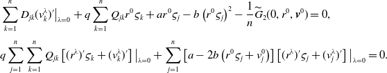 \begin{equation*} \begin{split} &\displaystyle \sum _{k=1}^n D_{jk}(v^\lambda _{k})'\big |_{\lambda =0}+q\sum _{k=1}^{n} Q_{jk}r^0\varsigma _k+ar^0 \varsigma _j - b \left (r^0\varsigma _j \right )^2-\frac{1}{n}\widetilde{G}_2(0,r^0,{{\boldsymbol{v}}}^0)=0,\\[3pt] &\displaystyle q\sum _{j=1}^n \sum _{k=1}^n Q_{jk}\left [(r^\lambda )'\varsigma _k+(v_k^\lambda )'\right ]\big |_{\lambda =0}+ \sum _{j=1}^n\left [a-2b\left (r^0\varsigma _j+v^0_j\right )\right ]\left [(r^\lambda )'\varsigma _j+(v_j^\lambda )'\right ]\big |_{\lambda =0}=0. \end{split} \end{equation*}
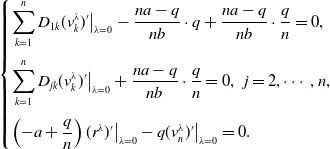
Noting that $r^0=\frac{na-q}{b}$
,
$r^0=\frac{na-q}{b}$
, $({{\boldsymbol{v}}}^\lambda )'\in \widetilde{X}_1$
and
$({{\boldsymbol{v}}}^\lambda )'\in \widetilde{X}_1$
and $\widetilde{G}_2(0,r^0,{{\boldsymbol{v}}}^0)=0$
, we have
$\widetilde{G}_2(0,r^0,{{\boldsymbol{v}}}^0)=0$
, we have
 \begin{equation*} \begin{cases} \displaystyle \sum _{k=1}^n D_{1k}(v^\lambda _{k})'\big |_{\lambda =0}-\frac{na-q}{nb}\cdot q+\frac{na-q}{nb}\cdot \frac{q}{n}=0,\\[15pt] \displaystyle \sum _{k=1}^n D_{jk}(v^\lambda _{k})'\big |_{\lambda =0}+\frac{na-q}{nb}\cdot \frac{q}{n}=0,\;\;j=2,\cdots, n,\\[15pt] \displaystyle \left (-a+\frac{q}{n}\right )(r^\lambda )'\big |_{\lambda =0}-q(v^\lambda _{n})'\big |_{\lambda =0}=0. \end{cases} \end{equation*}
By a tedious computation (see Proposition 5.4 in the appendix), we obtain that
 \begin{equation*} ( v^\lambda _n)'\big |_{\lambda =0}=\frac {q(na-q)(n+1)(n-1)}{6nb},\;\;(r^\lambda )'\big |_{\lambda =0}=-\frac {q^2(n+1)(n-1)}{6b}. \end{equation*}
This, combined with (2.24), implies that
 \begin{equation*} \displaystyle \sum _{j=1}^n (u^\lambda _j)'\big |_{\lambda =0}= (r^\lambda )'\big |_{\lambda =0}=-\frac {q^2(n+1)(n-1)}{6b}. \end{equation*}
This completes the proof.
Remark 2.7.
Note that $\lambda =1/d$
. Then the total population size
$\lambda =1/d$
. Then the total population size $\sum _{j=1}^n u_{d,j}$
for
(2.2) is strictly increasing in
$\sum _{j=1}^n u_{d,j}$
for
(2.2) is strictly increasing in $d\in [\delta, \infty )$
with
$d\in [\delta, \infty )$
with $\delta \gg 1$
.
$\delta \gg 1$
.
3. Eigenvalue problem
Linearising model (1.5) at ${\boldsymbol{u}}_d$
, we have
${\boldsymbol{u}}_d$
, we have
 \begin{equation} \displaystyle \frac{d{{\boldsymbol{v}}}}{d t}=dD{{\boldsymbol{v}}}+ q Q{{\boldsymbol{v}}}+\mathrm{diag}\left (a- b u_{d,j}\right ){{\boldsymbol{v}}}- \mathrm{diag}\left (b u_{d,j}\right ){{\boldsymbol{v}}}(t-\tau ).\\[5pt] \end{equation}
It follows from [Reference Hale21, Chapter 7] that the infinitesimal generator $A_{\tau }(d)$
of the solution semigroup of (3.1) is defined by:
$A_{\tau }(d)$
of the solution semigroup of (3.1) is defined by:
 \begin{equation} \begin{split} A_\tau (d)\boldsymbol{\Psi }=\dot{\boldsymbol{\Psi }} \end{split} \end{equation}
with the domain
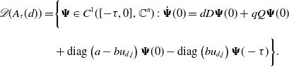 \begin{equation} {\begin{aligned} \mathscr{D}(A_\tau (d)) =&\bigg \{\boldsymbol{\Psi }\in C^1([\!-\!\tau, 0],\mathbb{C}^n)\;:\;\dot{\boldsymbol{\Psi }}(0)=dD \boldsymbol{\Psi }(0)+ q Q \boldsymbol{\Psi }(0)\\[5pt] &+\text{diag}\left (a- b u_{d,j}\right )\boldsymbol{\Psi }(0)- \text{diag}\left ( b u_{d,j}\right )\boldsymbol{\Psi }(-\tau )\bigg \}. \end{aligned}} \end{equation}
Then $\mu \in \sigma _p(A_\tau (d))$
(resp.,
$\mu \in \sigma _p(A_\tau (d))$
(resp., $\mu$
is an eigenvalue of
$\mu$
is an eigenvalue of $A_\tau (d)$
) if and only if there exists
$A_\tau (d)$
) if and only if there exists $\boldsymbol{\psi }=(\psi _1,\cdots, \psi _n)^T(\neq \textbf{0}) \in \mathbb{C}^n$
such that
$\boldsymbol{\psi }=(\psi _1,\cdots, \psi _n)^T(\neq \textbf{0}) \in \mathbb{C}^n$
such that $\triangle (d,\mu, \tau )\boldsymbol{\psi }=0$
, where matrix
$\triangle (d,\mu, \tau )\boldsymbol{\psi }=0$
, where matrix
 \begin{equation} \begin{split} \displaystyle \triangle (d,\mu, \tau )\;:\!=\;dD + q Q + \mathrm{diag}\left (a- b u_{d,j}\right )- e^{-\mu \tau }\mathrm{diag}\left ( b u_{d,j}\right )-\mu I. \end{split} \end{equation}
To determine the distribution of the eigenvalues of $A_\tau (d)$
, one need to consider whether
$A_\tau (d)$
, one need to consider whether
 \begin{equation*} \sigma _p(A_\tau (d))\cap \{x+\textrm {i} y:x=0\}\ne \emptyset . \end{equation*}
By Proposition 2.4, we have
 \begin{equation*} \begin{split} &0\not \in \sigma _p(A_\tau (d)) \;\;\text{for all}\;\;\tau \ge 0,\\[5pt] &\sigma _p(A_\tau (d))\subset \{x+\textrm{i} y:x\lt 0\}\;\; \text{for}\;\; \tau =0. \end{split} \end{equation*}
In fact, if $0\in \sigma _p(A_{\tau _0}(d))$
for some
$0\in \sigma _p(A_{\tau _0}(d))$
for some $\tau _0\ge 0$
, then
$\tau _0\ge 0$
, then $0$
is an eigenvalue of matrix
$0$
is an eigenvalue of matrix
 \begin{equation*}dD + q Q + \mathrm {diag}\left (a- 2b u_{d,j}\right ),\end{equation*}
which contradicts Proposition 2.4. By (3.4), we see that $\textrm{i}\nu (\nu \gt 0)\in \sigma _p(A_\tau (d))$
for some
$\textrm{i}\nu (\nu \gt 0)\in \sigma _p(A_\tau (d))$
for some $\tau \gt 0$
if and only if
$\tau \gt 0$
if and only if
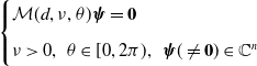 \begin{equation} \begin{cases} \mathcal M(d,\nu, \theta )\boldsymbol{\psi }=\textbf{0}\\[5pt] \nu \gt 0,\;\;\theta \in [0,2\pi ),\;\;\boldsymbol{\psi }(\neq \textbf{0}) \in \mathbb{C}^n \end{cases} \end{equation}
admits a solution $(\nu, \theta, \boldsymbol{\psi })$
, where matrix
$(\nu, \theta, \boldsymbol{\psi })$
, where matrix
 \begin{equation} \mathcal M(d,\nu, \theta )=d\displaystyle D + q Q +\mathrm{diag}\left (a- b u_{d,j}\right )- e^{-\textrm{i}\theta }\mathrm{diag}\left (b u_{d,j}\right )-\textrm{i}\nu I. \end{equation}
It follows from Proposition 2.5 that the properties of ${\boldsymbol{u}}_d$
are different for the following three cases (see Figure 3):
${\boldsymbol{u}}_d$
are different for the following three cases (see Figure 3):
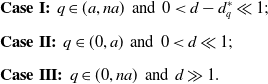 \begin{equation*} \begin{split} &{\textbf{Case I:}}\;\;q\in (a,na)\;\;\text{and}\;\;0\lt d-d_q^*\ll 1;\\[5pt] &{\textbf{Case II:}}\;\;q\in (0,a)\;\;\text{and}\;\;0\lt d\ll 1;\\[5pt] &{\textbf{Case III:}}\;\;q\in (0,na)\;\;\text{and}\;\;d\gg 1. \end{split} \end{equation*}
Therefore, the following analysis on eigenvalue problem (3.5) is divided into three cases.
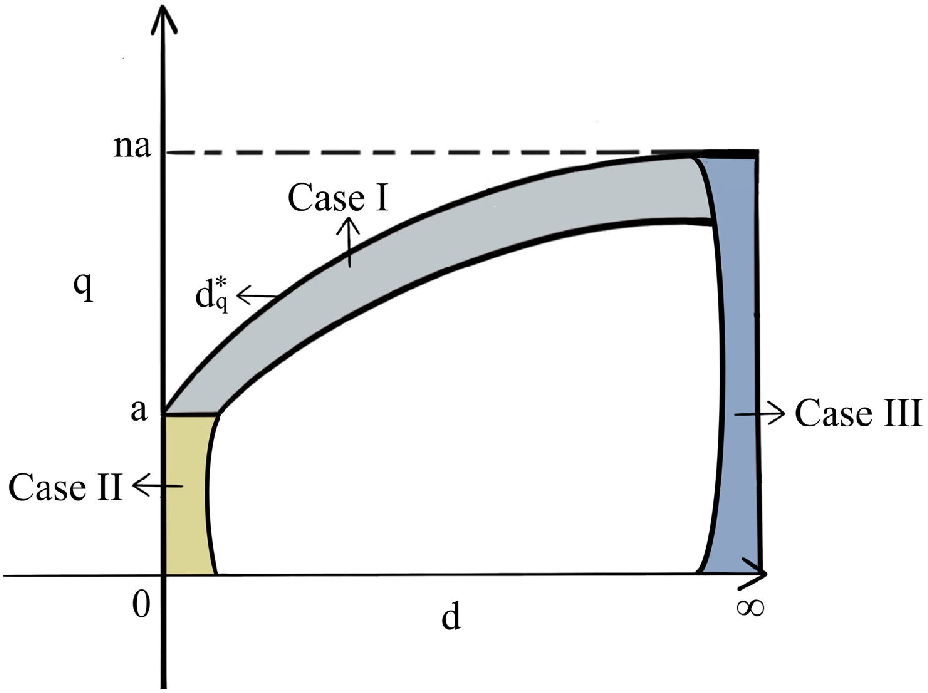
Figure 3. Diagram for parameter ranges of Cases I–III.
3.1. A priori estimates
In this subsection, we give a priori estimates for solutions of (3.5).
Lemma 3.1.
Let $\left (\nu ^{d}, \theta ^{d}, \boldsymbol{\psi }^{d}\right )$
be a solution of
(3.5). Then the following statements hold:
$\left (\nu ^{d}, \theta ^{d}, \boldsymbol{\psi }^{d}\right )$
be a solution of
(3.5). Then the following statements hold:
-
(i) For fixed
$q\in (a,na)$
,
$\left |\displaystyle \frac{\nu ^{d}}{d-d^*_q}\right |$
is bounded for
$d\in (d_q^*,\tilde d_1]$
with
$0\lt \tilde d_1-d_q^*\ll 1$
; -
(ii) For fixed
$q\in (0,a)$
,
$|\nu ^{d}|$
is bounded for
$d \in (0,\tilde d_2)$
with
$0\lt \tilde d_2\ll 1$
; -
(iii) For fixed
$q\in (0,na)$
,
$|\nu ^{d}|$
is bounded for
$d\in (\tilde d_3,\infty )$
with
$\tilde d_3\gg 1$
.


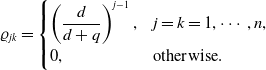
Proof. We only prove (i), and (ii)–(iii) can be proved similarly. Define matrix $\varrho \;:\!=\;\left (\varrho _{jk}\right )$
with
$\varrho \;:\!=\;\left (\varrho _{jk}\right )$
with
 \begin{eqnarray*} \varrho _{jk}= \begin{cases} \left (\displaystyle \frac{d}{d+q}\right )^{j-1}, & j=k=1,\cdots, n,\\[5pt] 0, &\text{otherwise}. \end{cases} \end{eqnarray*}
Substituting $(\nu, \theta, \boldsymbol \psi )=\left (\nu ^{d}, \theta ^{d}, \boldsymbol{\psi }^{d}\right )$
into (3.5), and multiplying both sides of (3.5) by
$(\nu, \theta, \boldsymbol \psi )=\left (\nu ^{d}, \theta ^{d}, \boldsymbol{\psi }^{d}\right )$
into (3.5), and multiplying both sides of (3.5) by $\left (\overline{\psi ^d_1},\overline{\psi ^d_2},\dots, \overline{\psi ^d_n}\right )\varrho$
to the left, we have
$\left (\overline{\psi ^d_1},\overline{\psi ^d_2},\dots, \overline{\psi ^d_n}\right )\varrho$
to the left, we have
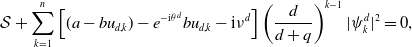 \begin{equation} \mathcal S+\sum _{k=1}^n\left [(a-bu_{d,k})-e^{-\textrm{i} \theta ^d}bu_{d,k}-\textrm{i}\nu ^d\right ]\left (\frac{d}{d+q}\right )^{k-1}|\psi ^d_k|^2=0, \end{equation}
where
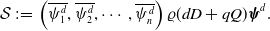 \begin{equation*} \mathcal S\;:\!=\;\left (\overline {\psi ^d_1},\overline {\psi ^d_2},\cdots, \overline {\psi ^d_n}\right )\varrho (dD+qQ)\boldsymbol \psi ^d. \end{equation*}
Since $\varrho (dD+qQ)$
is symmetric, we see that
$\varrho (dD+qQ)$
is symmetric, we see that $\mathcal S\in \mathbb{R}$
. This combined with (3.7) yields
$\mathcal S\in \mathbb{R}$
. This combined with (3.7) yields
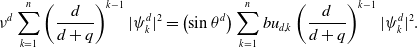 \begin{equation} \nu ^d\sum _{k=1}^{n}\left (\frac{d}{d+q}\right )^{k-1}|\psi ^d_k|^2=\left (\sin \theta ^d\right )\sum _{k=1}^{n}bu_{d,k}\left (\frac{d}{d+q}\right )^{k-1}|\psi ^d_k|^2. \end{equation}
By Proposition 2.5 (ii), we see that there exists $ M\gt 0$
such that
$ M\gt 0$
such that $\displaystyle \frac{\|{\boldsymbol{u}}_d\|_\infty }{d-d^*_q}\lt M$
for
$\displaystyle \frac{\|{\boldsymbol{u}}_d\|_\infty }{d-d^*_q}\lt M$
for $d\in (d^*_q,\tilde d_1]$
with
$d\in (d^*_q,\tilde d_1]$
with $0\lt \tilde d_1-d_q^*\ll 1$
. This combined with (3.8) implies that
$0\lt \tilde d_1-d_q^*\ll 1$
. This combined with (3.8) implies that
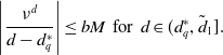 \begin{equation*} \left |\frac {\nu ^d}{d-d^*_q}\right |\le bM\;\;\text {for}\;\;d\in (d^{\ast}_q,\tilde d_1]. \end{equation*}
This completes the proof.
3.2. Case I
For this case, the positive equilibrium ${\boldsymbol{u}}_d$
can be represented as (2.10). Plugging (2.10) into (3.5), we rewrite the eigenvalue problem (3.5) as follows:
${\boldsymbol{u}}_d$
can be represented as (2.10). Plugging (2.10) into (3.5), we rewrite the eigenvalue problem (3.5) as follows:
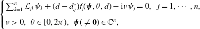 \begin{equation} \begin{cases} \sum _{k=1}^n \mathcal L_{jk}\psi _k+ (d-d_q^*)f_j(\boldsymbol{\psi },\theta, d)-\textrm{i}\nu \psi _j=0,\;\;\;j=1,\cdots, n,\\[5pt] \nu \gt 0,\;\;\theta \in [0,2\pi ),\;\;\boldsymbol{\psi }(\neq \textbf{0}) \in \mathbb{C}^n, \end{cases} \end{equation}
where $\mathcal L$
is defined in (2.3), and
$\mathcal L$
is defined in (2.3), and
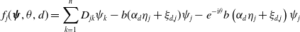 \begin{equation} f_j(\boldsymbol \psi, \theta, d)=\sum _{k=1}^n D_{jk}\psi _k-b( \alpha _d\eta _j+\xi _{d,j})\psi _j- e^{-\textrm{i}\theta }b\left (\alpha _d\eta _j+\xi _{d,j}\right )\psi _j \end{equation}
with $\alpha _d$
and
$\alpha _d$
and $\boldsymbol{\xi }_d$
defined in (2.10). By (2.6), we see that, ignoring a scalar factor,
$\boldsymbol{\xi }_d$
defined in (2.10). By (2.6), we see that, ignoring a scalar factor, $\boldsymbol{\psi } (\ne \textbf{0})\in \mathbb{C}^n$
in (3.9) can be represented as follows:
$\boldsymbol{\psi } (\ne \textbf{0})\in \mathbb{C}^n$
in (3.9) can be represented as follows:
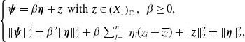 \begin{equation} \begin{cases} \boldsymbol{\psi }=\beta \boldsymbol{\eta }+{{\boldsymbol{z}}} \;\;\text{with}\;\;{{\boldsymbol{z}}} \in \left (X_{1}\right )_{\mathbb{C}}, \;\; \beta \geq 0, \\[5pt] \|\boldsymbol{\psi }\|_2^{2}=\beta ^2\|\boldsymbol{\eta }\|_2^2+\beta \sum _{j=1}^n\eta _i(z_i+\overline{z_i})+ \|{{\boldsymbol{z}}}\|_2^2=\|\boldsymbol{\eta }\|_2^2, \end{cases} \end{equation}
where $\boldsymbol{\eta }$
is defined in (2.4). Then we obtain an equivalent problem of (3.9) in the following.
$\boldsymbol{\eta }$
is defined in (2.4). Then we obtain an equivalent problem of (3.9) in the following.
Lemma 3.2.
Assume that $d\gt d_q^*$
and
$d\gt d_q^*$
and $q\in (a,na)$
. Then
$q\in (a,na)$
. Then $(\boldsymbol{\psi },\nu, \theta )$
solves
(3.9), where
$(\boldsymbol{\psi },\nu, \theta )$
solves
(3.9), where $\boldsymbol{\psi }$
is defined in
(3.11) and
$\boldsymbol{\psi }$
is defined in
(3.11) and $\nu =(d-d^*_q)\varpi$
, if and only if
$\nu =(d-d^*_q)\varpi$
, if and only if $(\beta, \varpi, \theta, {{\boldsymbol{z}}})$
solves
$(\beta, \varpi, \theta, {{\boldsymbol{z}}})$
solves
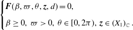 \begin{equation} \begin{cases}{{\boldsymbol{F}}}(\beta, \varpi, \theta, {{\boldsymbol{z}}},d)= 0,\\[5pt] \beta \ge 0,\;\varpi \gt 0,\;\theta \in [0,2\pi ),\;{{\boldsymbol{z}}}\in \left (X_{1}\right )_{\mathbb{C}}. \end{cases} \end{equation}
Here
 \begin{equation*} {{\boldsymbol{F}}}(\beta, \varpi, \theta, {{\boldsymbol{z}}},d)=( F_{1,1},\cdots, F_{1,n},F_2,F_3)^T\end{equation*}
is a continuously differentiable mapping from $\mathbb{R}^3\times \left (X_{1}\right )_{\mathbb{C}}\times [d^*_q,\infty ]$
to
$\mathbb{R}^3\times \left (X_{1}\right )_{\mathbb{C}}\times [d^*_q,\infty ]$
to $( X_{1})_{\mathbb{C}}\times \mathbb{C}\times \mathbb{R}$
, and
$( X_{1})_{\mathbb{C}}\times \mathbb{C}\times \mathbb{R}$
, and
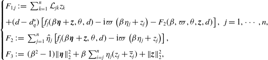 \begin{equation} \begin{cases} F_{1,j}\;:\!=\;\sum _{k=1}^n\mathcal L_{jk}z_k\\[5pt] +(d-d^*_q)\left [f_j(\beta \boldsymbol{\eta }+{{\boldsymbol{z}}},\theta, d)-\textrm{i}\varpi \left (\beta \eta _j+ z_j\right )-F_2(\beta, \varpi, \theta, {{{\boldsymbol{z}}}},d)\right ],\;\;j=1,\cdots, n,\\[5pt] F_2\;:\!=\;\sum _{j=1}^n\hat \eta _j\left [f_j(\beta \boldsymbol{\eta }+{{\boldsymbol{z}}},\theta, d)-\textrm{i}\varpi \left (\beta \eta _j+ z_j\right )\right ],\\[5pt] F_3\;:\!=\;(\beta ^2-1)\|\boldsymbol{\eta }\|_2^2+\beta \sum _{i=j}^n\eta _j(z_j+\overline z_j)+ \|{{\boldsymbol{z}}}\|_2^2, \end{cases} \end{equation}
where $f_j\;(j=1,\cdots, n)$
are defined in
(3.10).
$f_j\;(j=1,\cdots, n)$
are defined in
(3.10).
Proof. Clearly, $F_3=0$
is equivalent to second equation of (3.11). Substituting (3.11) and
$F_3=0$
is equivalent to second equation of (3.11). Substituting (3.11) and $\nu =(d-d^*_q)\varpi$
into (3.9), we see that
$\nu =(d-d^*_q)\varpi$
into (3.9), we see that
 \begin{equation} \sum _{k=1}^n \mathcal L_{jk}z_k+ (d-d^*_q)\left [f_j(\beta \boldsymbol{\eta }+{{\boldsymbol{z}}},\theta, d)-\textrm{i}\varpi \left (\beta \eta _j+ z_j\right )\right ]=0,\;\;\;j=1,\cdots, n. \end{equation}
Denote the left side of (3.14) by $y_j$
and let
$y_j$
and let ${{\boldsymbol{y}}}=(y_1,\cdots, y_n)^T$
. Using similar arguments as in the proof of Proposition 2.5 (ii), we see that
${{\boldsymbol{y}}}=(y_1,\cdots, y_n)^T$
. Using similar arguments as in the proof of Proposition 2.5 (ii), we see that ${{\boldsymbol{y}}}=\textbf{0}$
if and only
${{\boldsymbol{y}}}=\textbf{0}$
if and only $F_2=0$
and
$F_2=0$
and $\displaystyle F_{1,j}=0$
for all
$\displaystyle F_{1,j}=0$
for all $j=1,\cdots, n$
. This completes the proof.
$j=1,\cdots, n$
. This completes the proof.
We first show that the equivalent problem (3.12) has a unique solution for $d=d^*_q$
.
$d=d^*_q$
.
Lemma 3.3. The following equation
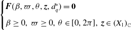 \begin{equation*} \begin{cases}{{\boldsymbol{F}}}(\beta, \varpi, \theta, {{{\boldsymbol{z}}}},d^*_q)=\textbf{0} \\[5pt] \beta \ge 0,\;\varpi \geq 0,\;\theta \in [0,2\pi ],\;{{\boldsymbol{z}}}\in \left (X_{1}\right )_{\mathbb{C}} \end{cases} \end{equation*}
has a unique solution $\left (\beta ^*, \varpi ^*,\theta ^*,{{\boldsymbol{z}}}^*\right )$
. Here
$\left (\beta ^*, \varpi ^*,\theta ^*,{{\boldsymbol{z}}}^*\right )$
. Here
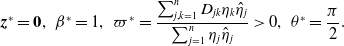 \begin{equation*} \begin{aligned}{{\boldsymbol{z}}}^*=\textbf{0},\;\; \beta ^*=1,\;\;\varpi ^*=\frac{\sum _{j,k=1}^nD_{jk}\eta _k\hat \eta _j}{\sum _{j=1}^n\eta _j\hat \eta _j}\gt 0,\;\;\theta ^*=\frac{\pi }{2}. \end{aligned} \end{equation*}
Proof. Clearly,
 \begin{equation*}F_{1,j}(\beta, \varpi, \theta, {{{\boldsymbol{z}}}},d^*_q)= 0\;\;\text {for all}\;\;j=1,\cdots, n\end{equation*}
if and only if ${{\boldsymbol{z}}}={{\boldsymbol{z}}}^*=\textbf{0}$
. Substituting
${{\boldsymbol{z}}}={{\boldsymbol{z}}}^*=\textbf{0}$
. Substituting ${{\boldsymbol{z}}}=\textbf{0}$
into
${{\boldsymbol{z}}}=\textbf{0}$
into $F_3(\beta, \varpi, \theta, {{{\boldsymbol{z}}}},d^*_q)= 0$
, we have
$F_3(\beta, \varpi, \theta, {{{\boldsymbol{z}}}},d^*_q)= 0$
, we have $\beta =\beta ^*=1$
. Then plugging
$\beta =\beta ^*=1$
. Then plugging ${{\boldsymbol{z}}}=\textbf{0}$
and
${{\boldsymbol{z}}}=\textbf{0}$
and $\beta =1$
into
$\beta =1$
into $F_2(\beta, \varpi, \theta, {{{\boldsymbol{z}}}},d^*_q)= 0$
, we have
$F_2(\beta, \varpi, \theta, {{{\boldsymbol{z}}}},d^*_q)= 0$
, we have
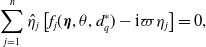 \begin{equation} \sum _{j=1}^n\hat \eta _j\left [f_j( \boldsymbol{\eta },\theta, d_q^*)-\textrm{i} \varpi \eta _j\right ]=0, \end{equation}
where $f_j\;(j=1,\cdots, n)$
are defined in (3.10). By Proposition 2.5 (ii), we have
$f_j\;(j=1,\cdots, n)$
are defined in (3.10). By Proposition 2.5 (ii), we have
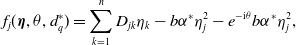 \begin{equation*}f_j( \boldsymbol {\eta },\theta, d_q^*)=\sum _{k=1}^n D_{jk}\eta _k-b\alpha ^*\eta ^2_j- e^{-\textrm {i}\theta }b\alpha ^*\eta ^2_j,\end{equation*}
where $\alpha ^*$
is defined in (2.11). Then we see from (3.15) that
$\alpha ^*$
is defined in (2.11). Then we see from (3.15) that
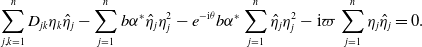 \begin{equation*} \sum _{j,k=1}^n D_{jk}\eta _k\hat \eta _j-\sum _{j=1}^n b\alpha ^*\hat \eta _{j}\eta _j^2-e^{-\textrm {i}\theta }b\alpha ^*\sum _{j=1}^n\hat \eta _{j}\eta _j^2-\textrm {i}\varpi \sum _{j=1}^n\eta _j\hat \eta _{j}=0. \end{equation*}
This combined with (2.11) yields
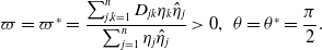 \begin{equation*}\varpi =\varpi ^*=\frac {\sum _{j,k=1}^nD_{jk}\eta _k\hat \eta _j}{\sum _{j=1}^n\eta _j\hat \eta _j}\gt 0, \;\;\theta =\theta ^*=\frac {\pi }{2}.\end{equation*}
This completes the proof.
Then we solve the equivalent problem (3.12) for $0\lt d-d^*_q\ll 1$
.
$0\lt d-d^*_q\ll 1$
.
Lemma 3.4.
Assume that $d\gt d_q^*$
and
$d\gt d_q^*$
and $q\in (a,na)$
. Then there exists
$q\in (a,na)$
. Then there exists $\tilde d_1$
with
$\tilde d_1$
with $0\lt \tilde d_1-d^*_q\ll 1$
and a continuously differentiable mapping
$0\lt \tilde d_1-d^*_q\ll 1$
and a continuously differentiable mapping $d\mapsto \left (\beta _d,\varpi _d,\theta _d,{{\boldsymbol{z}}}_d\right )$
from
$d\mapsto \left (\beta _d,\varpi _d,\theta _d,{{\boldsymbol{z}}}_d\right )$
from $[d^*_q,\tilde d_1]$
to
$[d^*_q,\tilde d_1]$
to $\mathbb{R}^{3}\times ({X}_{1})_{\mathbb{C}}$
such that
$\mathbb{R}^{3}\times ({X}_{1})_{\mathbb{C}}$
such that $(\beta _d,\varpi _d,\theta _d,{{\boldsymbol{z}}}_d)$
is the unique solution of the following problem:
$(\beta _d,\varpi _d,\theta _d,{{\boldsymbol{z}}}_d)$
is the unique solution of the following problem:
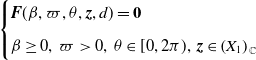 \begin{equation} \begin{cases}{{\boldsymbol{F}}}(\beta, \varpi, \theta, {{{\boldsymbol{z}}}},d)=\textbf{0} \\[5pt] \beta \ge 0,\;\varpi \gt 0,\;\theta \in [0,2\pi ),\;{{\boldsymbol{z}}}\in \left (X_{1}\right )_{\mathbb{C}} \end{cases} \end{equation}
for $d\in \left (d^*_q,\tilde d_1\right ]$
.
$d\in \left (d^*_q,\tilde d_1\right ]$
.
Proof. Let ${{\boldsymbol{P}}}\left (\check{\beta },\check{\varpi },\check{\theta },{\check{{{\boldsymbol{z}}}}}\right )=(P_{1,1}, \cdots, P_{1,n},P_2,P_3)^T \;:\; \mathbb{R}^3 \times (X_{1})_{\mathbb{C}} \mapsto (X_{1})_{\mathbb{C}}\times \mathbb{C}\times \mathbb{R}$
be the Fréchet derivative of
${{\boldsymbol{P}}}\left (\check{\beta },\check{\varpi },\check{\theta },{\check{{{\boldsymbol{z}}}}}\right )=(P_{1,1}, \cdots, P_{1,n},P_2,P_3)^T \;:\; \mathbb{R}^3 \times (X_{1})_{\mathbb{C}} \mapsto (X_{1})_{\mathbb{C}}\times \mathbb{C}\times \mathbb{R}$
be the Fréchet derivative of ${\boldsymbol{F}}$
with respect to
${\boldsymbol{F}}$
with respect to $(\beta, \varpi, \theta, {{{\boldsymbol{z}}}})$
at
$(\beta, \varpi, \theta, {{{\boldsymbol{z}}}})$
at $\left (\beta ^*, \varpi ^*,\theta ^*,{{\boldsymbol{z}}}^*,d^*_q\right )$
. It follows from (3.12) and (3.13) that
$\left (\beta ^*, \varpi ^*,\theta ^*,{{\boldsymbol{z}}}^*,d^*_q\right )$
. It follows from (3.12) and (3.13) that
 \begin{equation*} \begin{split} &P_{1,j}\left (\check{\beta },\check{\varpi },\check{\theta },{\check{{{\boldsymbol{z}}}}}\right )=\sum _{k=1}^{n} \mathcal L_{jk} \check{z}_{k},\;\;j=1,\cdots, n,\\[5pt] &P_{2}\left (\check{\beta },\check{\varpi },\check{\theta },{\check{{{\boldsymbol{z}}}}}\right )=\sum _{j=1}^{n}\hat \eta _j\left (\sum _{k=1}^{n}D_{jk}\check{z}_k -b\alpha ^*\eta _j\check{z}_j+\textrm{i}b\alpha ^*\eta _j\check{z}_j-\textrm{i}\varpi ^*\check{z}_j+b\alpha ^*\eta _j^2\check{\theta } - \mathrm{i}\eta _j\check{\varpi }\right )\\[5pt] & +\sum _{j=1}^{n}\hat \eta _j(\textrm{i}b\alpha ^*\eta _j^2\check \beta -\textrm{i}\varpi ^*\eta _j\check \beta ),\\[5pt] &P_{3}\left (\check{\beta },\check{\varpi },\check{\theta },{\check{{{\boldsymbol{z}}}}}\right )=2\|\eta \|^2_2\check{\beta }+\sum _{j=1}^{n}\eta _j\left (\check{z}_j+ \overline{\check{z}_j}\right ), \end{split} \end{equation*}
where we have used (2.11) to obtain $P_2$
. A direct computation implies that
$P_2$
. A direct computation implies that ${\boldsymbol{P}}$
is a bijection from
${\boldsymbol{P}}$
is a bijection from $\mathbb{R}^3 \times (X_{1})_{\mathbb{C}}$
to
$\mathbb{R}^3 \times (X_{1})_{\mathbb{C}}$
to $(X_{1})_{\mathbb{C}}\times \mathbb{C}\times \mathbb{R}$
. It follows from the implicit function theorem that there exists
$(X_{1})_{\mathbb{C}}\times \mathbb{C}\times \mathbb{R}$
. It follows from the implicit function theorem that there exists $\hat d\gt d^*_q$
and a continuously differentiable mapping
$\hat d\gt d^*_q$
and a continuously differentiable mapping $d\mapsto \left (\beta _d,\varpi _d,\theta _d,{{\boldsymbol{z}}}_d\right )$
from
$d\mapsto \left (\beta _d,\varpi _d,\theta _d,{{\boldsymbol{z}}}_d\right )$
from $\left [d^*_q,\hat d\right ]$
to
$\left [d^*_q,\hat d\right ]$
to $\mathbb{R}^3 \times (X_{1})_{\mathbb{C}}$
such that
$\mathbb{R}^3 \times (X_{1})_{\mathbb{C}}$
such that $\left (\beta _d,\varpi _d,\theta _d,{{\boldsymbol{z}}}_d\right )$
solves (3.16).
$\left (\beta _d,\varpi _d,\theta _d,{{\boldsymbol{z}}}_d\right )$
solves (3.16).
Then we prove the uniqueness for $d\in [d^*_q,\tilde d_1]$
with
$d\in [d^*_q,\tilde d_1]$
with $0\lt \tilde d_1-d^*_q\ll 1$
. We only need to verify that if
$0\lt \tilde d_1-d^*_q\ll 1$
. We only need to verify that if $\left (\beta ^d,\varpi ^d,\theta ^d,{{\boldsymbol{z}}}^d\right )$
satisfies (3.16), then
$\left (\beta ^d,\varpi ^d,\theta ^d,{{\boldsymbol{z}}}^d\right )$
satisfies (3.16), then $\lim _{d\rightarrow d^*_q}\left (\beta ^d,\varpi ^d,\theta ^d,{{\boldsymbol{z}}}^d\right )=\left (\beta ^*, \varpi ^*,\theta ^*,{{\boldsymbol{z}}}^*\right )$
, where
$\lim _{d\rightarrow d^*_q}\left (\beta ^d,\varpi ^d,\theta ^d,{{\boldsymbol{z}}}^d\right )=\left (\beta ^*, \varpi ^*,\theta ^*,{{\boldsymbol{z}}}^*\right )$
, where $\left (\beta ^*, \varpi ^*,\theta ^*,{{\boldsymbol{z}}}^*\right )$
is defined in Lemma 3.3. Since
$\left (\beta ^*, \varpi ^*,\theta ^*,{{\boldsymbol{z}}}^*\right )$
is defined in Lemma 3.3. Since
 \begin{equation*}F_3\left (\beta ^d,\varpi ^d,\theta ^d, {{\boldsymbol{z}}}^d,d\right )=0,\end{equation*}
we have
 \begin{equation} \| \beta ^d\boldsymbol{\eta }+{{\boldsymbol{z}}}^d\|_2^{2}=\|\boldsymbol{\eta }\|_2^2. \end{equation}
Note from Lemma 3.1 (i) that $\varpi ^d$
is bounded for
$\varpi ^d$
is bounded for $d\in \left [d^*_q,\tilde d_1\right ]$
. This combined with (3.17) and the first equation of (3.13) implies that
$d\in \left [d^*_q,\tilde d_1\right ]$
. This combined with (3.17) and the first equation of (3.13) implies that $\displaystyle \lim _{d\to d_q^*}\mathcal L{{\boldsymbol{z}}}=\textbf{0}$
, and consequently,
$\displaystyle \lim _{d\to d_q^*}\mathcal L{{\boldsymbol{z}}}=\textbf{0}$
, and consequently, $\displaystyle \lim _{d\to d_q^*}{{\boldsymbol{z}}}^d={{\boldsymbol{z}}}^*=\textbf{0}$
. By the third equation of (3.13), we obtain that
$\displaystyle \lim _{d\to d_q^*}{{\boldsymbol{z}}}^d={{\boldsymbol{z}}}^*=\textbf{0}$
. By the third equation of (3.13), we obtain that $\displaystyle \lim _{d\to d_q^*}\beta ^d=\beta ^*=1$
. Then, it follows from the second equation of (3.13) that
$\displaystyle \lim _{d\to d_q^*}\beta ^d=\beta ^*=1$
. Then, it follows from the second equation of (3.13) that $\displaystyle \lim _{d\to d_q^*}\theta ^d=\theta ^*$
and
$\displaystyle \lim _{d\to d_q^*}\theta ^d=\theta ^*$
and $\displaystyle \lim _{d\to d_q^*}\varpi ^d=\varpi ^*$
. This completes the proof.
$\displaystyle \lim _{d\to d_q^*}\varpi ^d=\varpi ^*$
. This completes the proof.
By Lemma 3.4, we obtain the following result.
Theorem 3.5.
Assume that $q\in (a,na)$
. Then for
$q\in (a,na)$
. Then for $d\in \left (d^*_q,\tilde d_1\right ]$
with
$d\in \left (d^*_q,\tilde d_1\right ]$
with $0\lt \tilde d_1-d^*_q\ll 1$
,
$0\lt \tilde d_1-d^*_q\ll 1$
, $\left (\nu, \tau, \boldsymbol{\psi }\right )$
satisfies the following equation:
$\left (\nu, \tau, \boldsymbol{\psi }\right )$
satisfies the following equation:
 \begin{equation} \begin{cases} \Delta (d,\mathrm{i}\nu, \tau )\boldsymbol{\psi }=\textbf{0}\\[5pt] \nu \gt 0, \;\;\tau \geq 0, \;\; \boldsymbol{\psi }(\neq \textbf{0}) \in \mathbb{C}^n \end{cases} \end{equation}
if and only if
 \begin{equation*} \nu =\nu _d=(d-d^*_q)\varpi _d,\;\;\boldsymbol \psi =c_1 \boldsymbol \psi _d,\;\;\tau =\tau _{d,l}=\frac {\theta _d+2l\pi }{\nu _d},\;\;l=0,1,2,\cdots, \end{equation*}
where $\boldsymbol \psi _d=\beta _d\boldsymbol{\eta }+{{\boldsymbol{z}}}_d$
,
$\boldsymbol \psi _d=\beta _d\boldsymbol{\eta }+{{\boldsymbol{z}}}_d$
, $c_1\in \mathbb{C}$
is a non-zero constant, and
$c_1\in \mathbb{C}$
is a non-zero constant, and $\beta _d$
,
$\beta _d$
, $\varpi _d$
,
$\varpi _d$
, $\theta _d$
and
$\theta _d$
and ${{\boldsymbol{z}}}_d$
are defined in Lemma 3.4
.
${{\boldsymbol{z}}}_d$
are defined in Lemma 3.4
.
3.3. Case II
For this case, the positive equilibrium ${\boldsymbol{u}}_d$
is continuously differentiable for
${\boldsymbol{u}}_d$
is continuously differentiable for $d\in [0,\infty )$
. We first solve the eigenvalue problem (3.5) for
$d\in [0,\infty )$
. We first solve the eigenvalue problem (3.5) for $d=0$
.
$d=0$
.
Lemma 3.6.
Let $\mathcal M(d,\nu, \theta )$
be defined in
(3.6), and let
$\mathcal M(d,\nu, \theta )$
be defined in
(3.6), and let
 \begin{equation*} \textrm {Ker} (\mathcal M(0,\nu, \theta ))\;:\!=\;\left \{\boldsymbol {\psi }\in \mathbb {C}^n\;:\;\mathcal M(0,\nu, \theta )\boldsymbol {\psi }=\textbf{0}\right \}. \end{equation*}
Assume that $q\in (0,a)$
. Then
$q\in (0,a)$
. Then
 \begin{equation} \left \{(\nu, \theta )\;:\;\nu \ge 0,\;\theta \in [0,2\pi ], \;\textrm{Ker} (\mathcal M(0,\nu, \theta ))\ne \{\textbf{0}\}\right \}=\left \{(\nu _p^0,\theta _p^0)\right \}_{p=1}^n, \end{equation}
where
 \begin{equation} \begin{split} \theta ^{0}_{p}=\displaystyle \arccos \frac{a-q-bu_{0,p}}{bu_{0,p}},\;\;\nu ^{0}_{p}=\sqrt{\left (bu_{0,p}\right )^{2}-\left (a-q-bu_{0,p}\right )^{2}} \end{split} \end{equation}
with
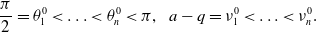 \begin{equation} \begin{split} \frac{\pi }{2}=\theta _1^0\lt \dots \lt \theta _n^0\lt \pi, \;\;\;a-q=\nu _1^0\lt \dots \lt \nu _n^0. \end{split} \end{equation}
Moreover, for each $p=1,2,\cdots, n$
,
$p=1,2,\cdots, n$
, $\textrm{Ker} (\mathcal M(0,\nu _p^0,\theta _p^0))=\left \{c\boldsymbol{\psi }^{0}_{p} \;:\; c\in \mathbb{C}\right \}$
, where
$\textrm{Ker} (\mathcal M(0,\nu _p^0,\theta _p^0))=\left \{c\boldsymbol{\psi }^{0}_{p} \;:\; c\in \mathbb{C}\right \}$
, where $\boldsymbol{\psi }^{0}_{p}=\left ({\psi }^{0}_{p,1},\cdots, {\psi }^{0}_{p,n}\right )^T$
, and
$\boldsymbol{\psi }^{0}_{p}=\left ({\psi }^{0}_{p,1},\cdots, {\psi }^{0}_{p,n}\right )^T$
, and
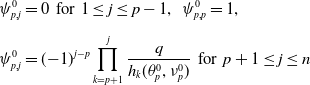 \begin{equation} \begin{split} &\psi ^{0}_{p,j}=0\;\;\text{for}\;\;1\le j\le p-1,\;\;\psi ^{0}_{p,p}=1,\\[5pt] &\psi ^{0}_{p,j}=(\!-\!1)^{j-p}\prod ^{j}_{k=p+1}\frac{q}{{h}_{k}(\theta ^{0}_{p},\nu ^0_{p})}\;\;\text{for}\;\;p+1\le j\le n \end{split} \end{equation}
with
 \begin{equation} h_k(\theta, \nu )=\left (a-q-bu_{0,k}\right ) -bu_{0,k}e^{-\textrm{i}\theta }-\textrm{i}\nu, \;\;k=1,\cdots, n. \end{equation}
Proof. Clearly, $\text{det}[M(d,\nu, \theta )]=\prod ^{n}_{p=1} h_p(\theta, \nu )$
. For each
$\text{det}[M(d,\nu, \theta )]=\prod ^{n}_{p=1} h_p(\theta, \nu )$
. For each $p=1,\cdots, n$
, we compute that
$p=1,\cdots, n$
, we compute that
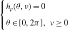 \begin{equation*} \begin{cases} h_p(\theta, \nu )=0\\[5pt] \theta \in [0,2\pi ],\;\;\nu \ge 0 \end{cases} \end{equation*}
admits a unique solution $(\nu _{p}^0,\theta _p^0)$
, which yields (3.19) holds. By (2.8) and (2.9), we see that (3.21) holds, and consequently,
$(\nu _{p}^0,\theta _p^0)$
, which yields (3.19) holds. By (2.8) and (2.9), we see that (3.21) holds, and consequently, ${h}_{k}(\theta ^{0}_{p},\nu ^0_{p})\ne 0$
for
${h}_{k}(\theta ^{0}_{p},\nu ^0_{p})\ne 0$
for $k\ne p$
, which implies that
$k\ne p$
, which implies that $\boldsymbol{\psi }^{0}_{p}$
is well defined for
$\boldsymbol{\psi }^{0}_{p}$
is well defined for $p=1,\cdots, n$
. A direct computation implies that
$p=1,\cdots, n$
. A direct computation implies that $\textrm{Ker} (\mathcal M(0,\nu _p^0,\theta _p^0))=\left \{c\boldsymbol{\psi }^{0}_{p}\;:\;c\in \mathbb{C}\right \}$
for
$\textrm{Ker} (\mathcal M(0,\nu _p^0,\theta _p^0))=\left \{c\boldsymbol{\psi }^{0}_{p}\;:\;c\in \mathbb{C}\right \}$
for $p=1,\cdots, n$
. This completes the proof.
$p=1,\cdots, n$
. This completes the proof.
The following result explores further properties of $(\nu ^{0}_{p},\theta ^{0}_{p})\;(p=1,\cdots, n)$
.
$(\nu ^{0}_{p},\theta ^{0}_{p})\;(p=1,\cdots, n)$
.
Lemma 3.7.
Assume that $q\in (0,a)$
, and let
$q\in (0,a)$
, and let $(\nu ^{0}_{p},\theta ^{0}_{p})\;(p=1,\cdots, n)$
be defined in
(3.20). Then the following statements hold:
$(\nu ^{0}_{p},\theta ^{0}_{p})\;(p=1,\cdots, n)$
be defined in
(3.20). Then the following statements hold:
-
(i)
$\displaystyle \frac{\theta ^{0}_{1}}{\nu ^{0}_{1}}\gt \displaystyle \frac{\theta ^{0}_{2}}{\nu ^{0}_{2}}\gt \dots \gt \displaystyle \frac{\theta ^{0}_{n}}{\nu ^{0}_{n}}$
; -
(ii) For all
$p=1,\cdots, n$
,
$\displaystyle \frac{\theta ^{0}_{p}}{\nu ^{0}_{p}}$
is strictly monotone increasing in
$q\in (0,a)$
and satisfies
$\displaystyle \lim _{q\to 0}\displaystyle \frac{\theta ^{0}_{p}}{\nu ^{0}_{p}}=\frac{\pi }{2a}$
.


Proof. By (3.20), we have
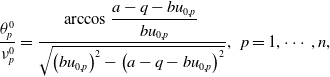 \begin{equation} \frac{\theta ^0_p}{\nu ^0_p}=\displaystyle \frac{\arccos \displaystyle \frac{a-q-bu_{0,p}}{bu_{0,p}}}{\sqrt{\left (bu_{0,p}\right )^{2} -\left (a-q-bu_{0,p}\right )^{2}}},\;\; p=1,\cdots, n, \end{equation}
where $u_{0,p}\ge (a-q)/b$
is defined in (2.8) and depends on
$u_{0,p}\ge (a-q)/b$
is defined in (2.8) and depends on $q$
for
$q$
for $p=1,\cdots, n$
. Then we denote
$p=1,\cdots, n$
. Then we denote $u_{0,p}$
by
$u_{0,p}$
by $u_{0,p}(q)$
throughout the proof. We define an auxiliary function
$u_{0,p}(q)$
throughout the proof. We define an auxiliary function
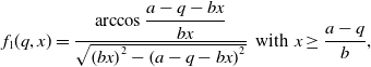 \begin{equation*} \displaystyle f_{1}(q,x)=\displaystyle \frac {\arccos \displaystyle \frac {a-q-bx}{bx}} {\sqrt {\left (bx\right )^{2}-\left (a-q-bx\right )^{2}}}\;\;\text {with}\;\;x\geq \frac {a-q}{b}, \end{equation*}
and consequently,
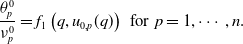 \begin{equation} \displaystyle \frac{\theta _{p}^0}{\nu _p^0}=f_1\left (q,u_{0,p}(q)\right ) \;\;\text{for}\;\; p=1,\cdots, n. \end{equation}
Let
 \begin{equation*}\displaystyle A_{1}=\arccos \frac {a-q-bx}{bx} \;\;\text {and}\;\;B_{1}=\sqrt {(bx)^{2}-\left (a-q-bx\right )^{2}}.\end{equation*}
Noticing that $q\in (0,a)$
, we compute that, for
$q\in (0,a)$
, we compute that, for $x\ge \displaystyle \frac{a-q}{b}$
,
$x\ge \displaystyle \frac{a-q}{b}$
,
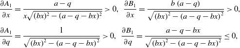 \begin{equation*} \begin{split} &\displaystyle \frac{\partial A_{1}}{\partial x}=\frac{a-q}{x\sqrt{(bx)^2-(a-q-bx)^2}}\gt 0,\;\; \displaystyle \frac{\partial B_{1}}{\partial x}=\frac{b\left (a-q\right )}{\sqrt{\left (bx\right )^{2}-\left (a-q-bx\right )^{2}}}\gt 0,\\[5pt] &\displaystyle \frac{\partial A_{1}}{\partial q}=\frac{1}{\sqrt{\left (bx\right )^{2}-\left (a-q-bx\right )^{2}}}\gt 0,\;\; \displaystyle \frac{\partial B_{1}}{\partial q}=\frac{a-q-bx}{\sqrt{\left (bx\right )^{2}-\left (a-q-bx\right )^{2}}}\le 0, \end{split} \end{equation*}
which yields
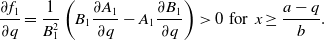 \begin{equation} \displaystyle \frac{\partial f_{1}}{\partial q}=\frac{1}{B_1^2}\left (B_{1}\displaystyle \frac{\partial A_{1}}{\partial q}-A_{1}\displaystyle \frac{\partial B_{1}}{\partial q}\right )\gt 0\;\;\text{for}\;\;x\geq \displaystyle \frac{a-q}{b}. \end{equation}
By $x\ge (a-q)/b$
and
$x\ge (a-q)/b$
and $q\in (0,a)$
again, we have
$q\in (0,a)$
again, we have
 \begin{equation*} 0\lt \frac {\sqrt {\left (bx\right )^{2}-\left (a-q-bx\right )^{2}}}{bx}\le 1\;\;\text {and}\;\;\arccos \frac {a-q-bx}{bx}\geq \frac {\pi }{2}, \end{equation*}
which yields
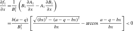 \begin{equation} \begin{split} \displaystyle \frac{\partial f_{1}}{\partial x}=&\frac{1}{B_1^2}\left (B_{1}\displaystyle \frac{\partial A_{1}}{\partial x}-A_{1}\displaystyle \frac{\partial B_{1}}{\partial x}\right )\\[5pt] =&\displaystyle \frac{b(a-q)}{B_1^3}\left [\frac{\sqrt{\left (bx\right )^{2}-\left (a-q-bx\right )^{2}}}{bx}-\arccos \frac{a-q-bx}{bx}\right ]\lt 0 \end{split} \end{equation}
for $x\geq (a-q)/b$
.
$x\geq (a-q)/b$
.
Now we prove (i). By Proposition 2.5, we have $u_{0,1}\lt \cdots \lt u_{0,n}$
. This combined with (3.25) and (3.27) implies that (i) holds. Then we consider (ii). We first show that
$u_{0,1}\lt \cdots \lt u_{0,n}$
. This combined with (3.25) and (3.27) implies that (i) holds. Then we consider (ii). We first show that $u_{0,p}'(q)\lt 0$
for
$u_{0,p}'(q)\lt 0$
for $q\gt 0$
and
$q\gt 0$
and $p=1,\cdots, n$
. Here,
$p=1,\cdots, n$
. Here, $'$
is the derivative with respect to
$'$
is the derivative with respect to $q$
. Differentiating (2.8) with respect to
$q$
. Differentiating (2.8) with respect to $q$
yields
$q$
yields
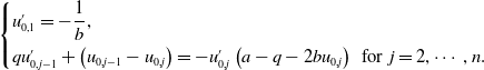 \begin{equation*} \begin{cases} u'_{0,1}=\displaystyle -\frac{1}{b},\\[5pt] qu'_{0,j-1}+\left (u_{0,j-1}-u_{0,j}\right )=-u'_{0,j}\left (a-q-2bu_{0,j}\right )\;\;\text{for}\;\;j=2,\cdots, n. \end{cases} \end{equation*}
This combined with the fact that
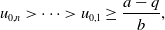 \begin{equation*}u_{0,n}\gt \cdots \gt u_{0,1}\ge \frac {a-q}{b},\end{equation*}
yields $u_{0,p}'(q)\lt 0$
for
$u_{0,p}'(q)\lt 0$
for $q\gt 0$
and
$q\gt 0$
and $p=1,\cdots, n$
. Then, by (3.25)–(3.27), we obtain that, for each
$p=1,\cdots, n$
. Then, by (3.25)–(3.27), we obtain that, for each $p=1,\cdots, n$
,
$p=1,\cdots, n$
,
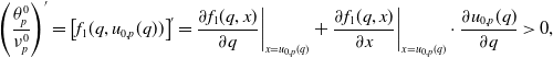 \begin{equation*} \left (\frac {\theta ^{0}_{p}}{\nu ^{0}_{p}}\right )'=\left [f_{1}(q,u_{0,p}(q))\right ]'=\frac {\partial f_{1}(q,x)}{\partial q}\bigg |_{x=u_{0,p}(q)}+\frac {\partial f_{1}(q,x)}{\partial x}\bigg |_{x=u_{0,p}(q)}\cdot \frac {\partial u_{0,p}(q)}{\partial q}\gt 0, \end{equation*}
where $'$
is the derivative with respect to
$'$
is the derivative with respect to $q$
. Note that
$q$
. Note that $\displaystyle \lim _{q\to 0}u_{0,p}(q)=a/b$
for
$\displaystyle \lim _{q\to 0}u_{0,p}(q)=a/b$
for $p=1,\cdots, n$
. Then, by (3.24), we have
$p=1,\cdots, n$
. Then, by (3.24), we have $\displaystyle \lim _{q\to 0}\displaystyle \frac{\theta ^{0}_{p}}{\nu ^{0}_{p}}=\frac{\pi }{2a}$
for
$\displaystyle \lim _{q\to 0}\displaystyle \frac{\theta ^{0}_{p}}{\nu ^{0}_{p}}=\frac{\pi }{2a}$
for $p=1,\cdots, n$
. This completes the proof.
$p=1,\cdots, n$
. This completes the proof.
Then we consider the solutions of (3.5) for $d\ne 0$
.
$d\ne 0$
.
Lemma 3.8.
Let $\mathcal M(d,\nu, \theta )$
be defined in
(3.6), and let
$\mathcal M(d,\nu, \theta )$
be defined in
(3.6), and let
 \begin{equation*} \textrm {Ker}(\mathcal M(d,\nu, \theta ))\;:\!=\;\left \{\boldsymbol {\psi }\in \mathbb {C}^n\;:\;\mathcal M(d,\nu, \theta )\boldsymbol {\psi }=\textbf{0}\right \}. \end{equation*}
Then there exists $\tilde{d}_2\gt 0$
such that, for
$\tilde{d}_2\gt 0$
such that, for $d\in (0,\tilde{d}_2]$
,
$d\in (0,\tilde{d}_2]$
,
 \begin{equation} W\;:\!=\;\left \{(\nu, \theta )\;:\;\nu \gt 0,\;\theta \in [0,2\pi ), \;\textrm{Ker}(\mathcal M(d,\nu, \theta ))\ne \{\textbf{0}\}\right \}=\left \{(\nu _p^d,\theta _p^d)\right \}_{p=1}^n, \end{equation}
where $(\nu ^{d}_{p},\theta ^{d}_{p}) \in (0,\infty )\times (0,\pi )$
for each
$(\nu ^{d}_{p},\theta ^{d}_{p}) \in (0,\infty )\times (0,\pi )$
for each $p=1,\cdots, n$
. Moreover, for each
$p=1,\cdots, n$
. Moreover, for each $p=1,\cdots, n$
,
$p=1,\cdots, n$
,
 \begin{equation} \textrm{Ker}(\mathcal M(d,\nu _p^d,\theta _p^d))=\left \{c\boldsymbol{\psi }^{d}_{p}\;:\;c\in \mathbb{C}\right \}, \end{equation}
where $(\nu ^{d}_{p},\theta ^{d}_{p},\boldsymbol{\psi }^{d}_{p})$
satisfies
$(\nu ^{d}_{p},\theta ^{d}_{p},\boldsymbol{\psi }^{d}_{p})$
satisfies $\lim _{d\to 0}(\nu ^{d}_{p},\theta ^{d}_{p},\boldsymbol{\psi }^{d}_{p})=\left (\nu ^{0}_{p},\theta ^{0}_{p},\boldsymbol{\psi }^{0}_{p}\right )$
, and
$\lim _{d\to 0}(\nu ^{d}_{p},\theta ^{d}_{p},\boldsymbol{\psi }^{d}_{p})=\left (\nu ^{0}_{p},\theta ^{0}_{p},\boldsymbol{\psi }^{0}_{p}\right )$
, and $\left (\nu ^{0}_{p},\theta ^{0}_{p},\boldsymbol{\psi }^{0}_{p}\right )$
is defined in Lemma 3.6
.
$\left (\nu ^{0}_{p},\theta ^{0}_{p},\boldsymbol{\psi }^{0}_{p}\right )$
is defined in Lemma 3.6
.
Proof.
Step 1. We show the existence of $\left \{(\nu _p^d,\theta _p^d)\right \}_{p=1}^n$
such that
$\left \{(\nu _p^d,\theta _p^d)\right \}_{p=1}^n$
such that $\left \{(\nu _p^d,\theta _p^d)\right \}_{p=1}^n\subset W$
.
$\left \{(\nu _p^d,\theta _p^d)\right \}_{p=1}^n\subset W$
.
We only consider the existence of $(\nu _2^d,\theta _2^d)$
, and
$(\nu _2^d,\theta _2^d)$
, and $\{(\nu ^{d}_{p},\theta ^{d}_{p})\}_{p\ne 2}$
can be obtained similarly. Letting
$\{(\nu ^{d}_{p},\theta ^{d}_{p})\}_{p\ne 2}$
can be obtained similarly. Letting $\mathcal M^H(d,\nu, \theta )$
be the conjugate transpose of
$\mathcal M^H(d,\nu, \theta )$
be the conjugate transpose of $\mathcal M(d,\nu, \theta )$
, we compute that
$\mathcal M(d,\nu, \theta )$
, we compute that
 \begin{equation*} \textrm {Ker}\left (\mathcal M^H(0,\nu _2^0,\theta _2^0)\right )\;:\!=\;\{\boldsymbol {\psi }\in \mathbb {C}^n\;:\;\mathcal M^H(0,\nu _2^0,\theta _2^0)\boldsymbol {\psi }=\textbf{0}\}=\left \{c {\boldsymbol {\varphi }}_2^0\;:\;c\in \mathbb {C}\right \}, \end{equation*}
where ${\boldsymbol{\varphi }}_2^0=\left (\varphi _{2,1}^0,\cdots, \varphi _{2,n}^0\right )^T$
with
${\boldsymbol{\varphi }}_2^0=\left (\varphi _{2,1}^0,\cdots, \varphi _{2,n}^0\right )^T$
with
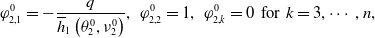 \begin{equation} \varphi _{2,1}^0=-\frac{q}{\overline{{h}}_1\left (\theta ^0_2,\nu ^0_2\right )}, \;\;\varphi _{2,2}^0=1,\;\;\varphi _{2,k}^0=0\;\;\text{for}\;\; k=3,\cdots, n, \end{equation}
and $\overline{{h}}_1\left (\theta ^0_2,\nu ^0_2\right )$
is the conjugate of
$\overline{{h}}_1\left (\theta ^0_2,\nu ^0_2\right )$
is the conjugate of $h_1\left (\theta ^0_2,\nu ^0_2\right )$
. By Lemma 3.6, we see that
$h_1\left (\theta ^0_2,\nu ^0_2\right )$
. By Lemma 3.6, we see that
 \begin{equation*}\textrm {Ker} (\mathcal M(0,\nu _2^0,\theta _2^0))=\left \{c\boldsymbol {\psi }^{0}_{2}\;:\;c\in \mathbb {C}\right \}.\end{equation*}
By (3.22) and (3.30), we see that
 \begin{equation} \langle{\boldsymbol{\varphi }}_2^0,\boldsymbol \psi _2^0\rangle =1, \end{equation}
and consequently
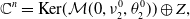 \begin{equation} \mathbb{C}^n=\textrm{Ker}(\mathcal M(0,\nu _2^0,\theta _2^0))\oplus Z, \end{equation}
where
 \begin{equation*} Z\;:\!=\;\left \{{{{\boldsymbol{z}}}}=(z_1,\cdots, z_n)^T \in \mathbb {C}^n\;:\;\langle {\boldsymbol \varphi }^{0}_{2},{{{\boldsymbol{z}}}}\rangle =0\right \}. \end{equation*}
Then by (3.30), (3.31) and (3.32), we see that, for any ${{\boldsymbol{y}}}\in \mathbb{C}^n$
,
${{\boldsymbol{y}}}\in \mathbb{C}^n$
,
 \begin{equation} {{\boldsymbol{y}}}=\widehat{c}{\boldsymbol{\psi }}_2^0+{{\boldsymbol{z}}}\;\; \text{with}\;\; \widehat{c}={\langle \boldsymbol{\varphi }^{0}_{2},{{\boldsymbol{y}}}\rangle }=\overline{\varphi }^{0}_{2,1}y_1+y_2 \;\;\text{and}\;\;{{\boldsymbol{z}}}\in Z, \end{equation}
where $\overline{\varphi }^{0}_{2,1}$
is the conjugate of
$\overline{\varphi }^{0}_{2,1}$
is the conjugate of $\varphi ^{0}_{2,1}$
.
$\varphi ^{0}_{2,1}$
.
Let
 \begin{equation} {{\boldsymbol{H}}}\left (d,\nu, \theta, {\boldsymbol{z}}\right )=(H_{1},\cdots, H_{n})^T\;:\!=\;\mathcal M\left (d,\nu, \theta \right )\left (\boldsymbol{\psi }^{0}_{2}+{\boldsymbol{z}}\right )\;:\;\mathbb{R}^{3}\times Z\rightarrow \mathbb{C}^n, \end{equation}
where matrix $\mathcal M\left (d,\nu, \theta \right )$
is defined in (3.6). By Lemma 3.6, we have
$\mathcal M\left (d,\nu, \theta \right )$
is defined in (3.6). By Lemma 3.6, we have ${{\boldsymbol{H}}}\left (0,\nu ^{0}_{2},\theta ^{0}_{2},\textbf{0}\right )=\textbf{0}$
, and then we solve
${{\boldsymbol{H}}}\left (0,\nu ^{0}_{2},\theta ^{0}_{2},\textbf{0}\right )=\textbf{0}$
, and then we solve ${{\boldsymbol{H}}}\left (d,\nu, \theta, {\boldsymbol{z}}\right )=\textbf{0}$
for
${{\boldsymbol{H}}}\left (d,\nu, \theta, {\boldsymbol{z}}\right )=\textbf{0}$
for $d\ne 0$
. By (3.32) and (3.33), we see that
$d\ne 0$
. By (3.32) and (3.33), we see that ${{\boldsymbol{H}}}\left (d,\nu, \theta, {\boldsymbol{z}}\right )=\textbf{0}$
if and only if
${{\boldsymbol{H}}}\left (d,\nu, \theta, {\boldsymbol{z}}\right )=\textbf{0}$
if and only if $\widetilde{{{\boldsymbol{H}}}}\left (d,\nu, \theta, {\boldsymbol{z}}\right )=\textbf{0}$
, where
$\widetilde{{{\boldsymbol{H}}}}\left (d,\nu, \theta, {\boldsymbol{z}}\right )=\textbf{0}$
, where
 \begin{equation*} \widetilde {{{\boldsymbol{H}}}}\left (d,\nu, \theta, \textbf{0}\right )=(\widetilde {H}_0,\widetilde H_{1,1},\cdots, \widetilde H_{1,n})^T \;:\; \mathbb {R}^{3}\times Z\rightarrow \mathbb {C}\times Z, \end{equation*}
and
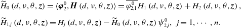 \begin{equation} \begin{split} &\widetilde H_{0}\left (d,\nu, \theta, {\boldsymbol{z}}\right )=\langle \boldsymbol \varphi ^{0}_{2},{{\boldsymbol{H}}}\left (d,\nu, \theta, {\boldsymbol{z}}\right )\rangle =\overline{\varphi ^{0}_{2,1}}H_1\left (d,\nu, \theta, {\boldsymbol{z}} \right )+H_2\left (d,\nu, \theta, {\boldsymbol{z}}\right ),\\[5pt] &\widetilde H_{1,j}\left (d,\nu, \theta, {\boldsymbol{z}}\right )=H_{j}\left (d,\nu, \theta, {\boldsymbol{z}}\right )-\widetilde H_0\left (d,\nu, \theta, {\boldsymbol{z}}\right )\psi _{2,j}^0,\;\;j=1,\cdots, n.\\[5pt] \end{split} \end{equation}
Let
 \begin{equation*}{{\boldsymbol{P}}}\left (\check {\nu },\check {\theta },\check {{\boldsymbol{z}}}\right )=(P_0,P_{1,1},\cdots, P_{1,n})^T\;:\;\mathbb {R}^2\times Z\to \mathbb {C}\times Z\end{equation*}
be the Fréchet derivative of $\widetilde{{{\boldsymbol{H}}}}$
with respect to
$\widetilde{{{\boldsymbol{H}}}}$
with respect to $\left (\nu, \theta, {\boldsymbol{z}}\right )$
at
$\left (\nu, \theta, {\boldsymbol{z}}\right )$
at $\left (0,\nu ^{0}_{2},\theta ^{0}_{2},\textbf{0}\right )$
. By (3.23) and the first equation of (3.35), we have
$\left (0,\nu ^{0}_{2},\theta ^{0}_{2},\textbf{0}\right )$
. By (3.23) and the first equation of (3.35), we have
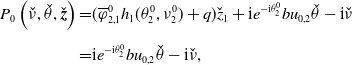 \begin{equation*} \begin{split} P_0\left (\check{\nu },\check{\theta },\check{{\boldsymbol{z}}}\right )=&(\overline{\varphi }^{0}_{2,1}h_1(\theta _2^0,\nu _2^0)+q)\check z_1+\textrm{i}e^{-\textrm{i}\theta ^0_2}bu_{0,2}\check{\theta }-\textrm{i}\check{\nu }\\[5pt] =&\textrm{i}e^{-\textrm{i}\theta ^0_2}bu_{0,2}\check{\theta }-\textrm{i}\check{\nu }, \end{split} \end{equation*}
where we have used (3.30) in the last step. By (3.23) and the second equation of (3.35), we have
 \begin{eqnarray*} \begin{aligned} &(P_{1,1},\cdots, P_{1,n})^T\left (\check{\nu },\check{\theta },\check{{\boldsymbol{z}}}\right )\\[5pt] =&\mathcal M(0,\theta _2^0,\nu _2^0)\check{{{\boldsymbol{z}}}}\\[5pt] &+\left (0,0,\left (\textrm{i}e^{-\textrm{i}\theta ^0_2} bu_{0,3}\check{\theta }-\textrm{i}e^{-\textrm{i}\theta ^0_2}bu_{0,2}\check{\theta }\right )\psi ^0_{2,3},\cdots, \left (\textrm{i}e^{-\textrm{i}\theta ^0_2} bu_{0,n}\check{\theta }-\textrm{i}e^{-\textrm{i}\theta ^0_2}bu_{0,2}\check{\theta }\right )\psi ^0_{2,n}\right )^T. \end{aligned} \end{eqnarray*}
Since $\mathcal M(0,\theta _2^0,\nu _2^0)$
is a bijection from
$\mathcal M(0,\theta _2^0,\nu _2^0)$
is a bijection from $Z$
to
$Z$
to $Z$
, it follows that
$Z$
, it follows that ${\boldsymbol{P}}$
is a bijection. Then we see from the implicit function theorem that there exists a constant
${\boldsymbol{P}}$
is a bijection. Then we see from the implicit function theorem that there exists a constant $\tilde d\gt 0$
, a neighbourhood
$\tilde d\gt 0$
, a neighbourhood $N_{2}$
of
$N_{2}$
of $\left (\nu ^{0}_{2},\theta ^{0}_{2},\textbf{0}\right )$
and a continuously differentiable function:
$\left (\nu ^{0}_{2},\theta ^{0}_{2},\textbf{0}\right )$
and a continuously differentiable function:
 \begin{equation*} \left (\nu ^{d}_{2},\theta ^{d}_{2},{\boldsymbol{z}}_2^{d}\right ):[0,\tilde d )\mapsto N_{2} \end{equation*}
such that for any $d\in [0,\tilde d)$
,
$d\in [0,\tilde d)$
, $\left (\nu ^{d}_{2},\theta ^{d}_{2},{\boldsymbol{z}}_2^{d}\right )$
is the unique solution of
$\left (\nu ^{d}_{2},\theta ^{d}_{2},{\boldsymbol{z}}_2^{d}\right )$
is the unique solution of $\widetilde{{{\boldsymbol{H}}}}\left (d,\nu, \theta, {\boldsymbol{z}}\right )=\textbf{0}$
in
$\widetilde{{{\boldsymbol{H}}}}\left (d,\nu, \theta, {\boldsymbol{z}}\right )=\textbf{0}$
in $N_{2}$
. Therefore,
$N_{2}$
. Therefore, $\left (\nu ^{d}_{2},\theta ^{d}_{2},{\boldsymbol{z}}_2^{d}\right )$
is also the unique solution of
$\left (\nu ^{d}_{2},\theta ^{d}_{2},{\boldsymbol{z}}_2^{d}\right )$
is also the unique solution of ${{\boldsymbol{H}}}\left (d,\nu, \theta, {\boldsymbol{z}}\right )=\textbf{0}$
in
${{\boldsymbol{H}}}\left (d,\nu, \theta, {\boldsymbol{z}}\right )=\textbf{0}$
in $N_{2}$
for
$N_{2}$
for $d\in [0,\tilde d)$
. This combined with (3.34) implies that
$d\in [0,\tilde d)$
. This combined with (3.34) implies that
 \begin{equation} \textrm{span}(\boldsymbol{\psi }^{d}_{2})\subset \textrm{Ker}(\mathcal M(d,\nu _2^d,\theta _2^d ))\;\;\text{for} \;\;d\in [0,\tilde d), \end{equation}
where $\boldsymbol{\psi }^{d}_{2}=\boldsymbol{\psi }^{0}_{2}+{\boldsymbol{z}}_2^{d}$
. Note that the rank of
$\boldsymbol{\psi }^{d}_{2}=\boldsymbol{\psi }^{0}_{2}+{\boldsymbol{z}}_2^{d}$
. Note that the rank of $\mathcal M(d,\nu _2^d,\theta _2^d)$
is
$\mathcal M(d,\nu _2^d,\theta _2^d)$
is $n-1$
. This combined with (3.36) implies that (3.29) holds. Therefore, we show the existence of
$n-1$
. This combined with (3.36) implies that (3.29) holds. Therefore, we show the existence of $(\nu ^{d}_{2},\theta ^{d}_{2})$
. Moreover,
$(\nu ^{d}_{2},\theta ^{d}_{2})$
. Moreover, $\displaystyle \lim _{d\to 0}(\nu ^{d}_{2},\theta ^{d}_{2},\boldsymbol{\psi }^{d}_{2})=\left (\nu ^{0}_{2},\theta ^{0}_{2},\boldsymbol{\psi }^{0}_{2}\right )$
. This combined with (3.21) implies that
$\displaystyle \lim _{d\to 0}(\nu ^{d}_{2},\theta ^{d}_{2},\boldsymbol{\psi }^{d}_{2})=\left (\nu ^{0}_{2},\theta ^{0}_{2},\boldsymbol{\psi }^{0}_{2}\right )$
. This combined with (3.21) implies that $(\nu ^{d}_{2},\theta ^{d}_{2}) \in (0,\infty )\times (0,\pi )$
.
$(\nu ^{d}_{2},\theta ^{d}_{2}) \in (0,\infty )\times (0,\pi )$
.
Step 2. We show that there exists $\tilde d_2$
such that (3.28) holds for
$\tilde d_2$
such that (3.28) holds for $d\in (0,\tilde d_2]$
.
$d\in (0,\tilde d_2]$
.
If it is not true, then there exist sequences $\left \{d_{j}\right \}^{\infty }_{j=1}$
and
$\left \{d_{j}\right \}^{\infty }_{j=1}$
and $\left \{\left (\nu ^{d_{j}},\theta ^{d_{j}}, \boldsymbol{\psi }^{d_{j}}\right )\right \}^{\infty }_{j=1}$
such that
$\left \{\left (\nu ^{d_{j}},\theta ^{d_{j}}, \boldsymbol{\psi }^{d_{j}}\right )\right \}^{\infty }_{j=1}$
such that $\displaystyle \lim _{j\rightarrow \infty }d_{j}=0$
, and for each
$\displaystyle \lim _{j\rightarrow \infty }d_{j}=0$
, and for each $j$
,
$j$
,
 \begin{equation*}\left (\nu ^{d_{j}},\theta ^{d_{j}}\right )\not \in \left \{\left (\nu ^{d_{j}}_{p},\theta ^{d_{j}}_{p}\right )\right \}_{p=1}^n,\;\; \|\boldsymbol {\psi }^{d_{j}}\|_{2}=1,\;\; \nu ^{d_{j}}\gt 0,\;\; \theta ^{d_{j}}\in \left [0,2\pi \right ),\end{equation*}
and
 \begin{equation} \mathcal M\left (d_{j},\nu ^{d_{j}},\theta ^{d_{j}}\right )\boldsymbol{\psi }^{d_{j}}=\textbf{0}. \end{equation}
It follows from Lemma 3.1 (ii) that $\nu ^{d_{j}}$
is bounded. Then, up to a subsequence, we have
$\nu ^{d_{j}}$
is bounded. Then, up to a subsequence, we have
 \begin{equation*} \lim _{j \rightarrow \infty }\theta ^{d_{j}}=\theta ^{*},\;\;\lim _{j\rightarrow \infty }\nu ^{d_{j}}=\nu ^{*}, \;\;\lim _{j\rightarrow \infty }\boldsymbol {\psi }^{d_{j}}=\boldsymbol {\psi }^{*} \end{equation*}
with $\theta ^*\in [0,2\pi ]$
,
$\theta ^*\in [0,2\pi ]$
, $\nu ^{*}\ge 0$
and
$\nu ^{*}\ge 0$
and $\|\boldsymbol{\psi }^{*}\|_2=1$
. Taking
$\|\boldsymbol{\psi }^{*}\|_2=1$
. Taking $j\to \infty$
on both sides of (3.37), we have
$j\to \infty$
on both sides of (3.37), we have $\mathcal M\left (0,\nu ^{*},\theta ^{*}\right )\boldsymbol{\psi }^{*}=\textbf{0}$
. This combined with Lemma 3.6 implies that there exists
$\mathcal M\left (0,\nu ^{*},\theta ^{*}\right )\boldsymbol{\psi }^{*}=\textbf{0}$
. This combined with Lemma 3.6 implies that there exists $1\leq p_{0}\leq n$
and a constant
$1\leq p_{0}\leq n$
and a constant $c_{p_{0}}\ne 0$
such that
$c_{p_{0}}\ne 0$
such that $\nu ^{*}=\nu ^{0}_{p_{0}}$
and
$\nu ^{*}=\nu ^{0}_{p_{0}}$
and $\theta ^{*}=\theta ^{0}_{p_{0}}$
,
$\theta ^{*}=\theta ^{0}_{p_{0}}$
, $\boldsymbol{\psi }^{*}=c_{p_{0}}\boldsymbol{\psi }^{0}_{p_{0}}$
. Without loss of generality, we assume that
$\boldsymbol{\psi }^{*}=c_{p_{0}}\boldsymbol{\psi }^{0}_{p_{0}}$
. Without loss of generality, we assume that $p_0=2$
. Then, for sufficiently large
$p_0=2$
. Then, for sufficiently large $j$
,
$j$
,
 \begin{equation*} \left (\nu ^{d_{j}},\theta ^{d_{j}},\frac {1}{c_{2}}\boldsymbol {\psi }^{d_{j}}-\boldsymbol {\psi }^{0}_{2}\right )\in N_{2}, \end{equation*}
where $N_{2}$
(defined in step 1) is a neighbourhood of
$N_{2}$
(defined in step 1) is a neighbourhood of $\left (\nu ^{0}_{2},\theta ^{0}_{2},\textbf{0}\right )$
. By (3.34) and (3.37), we see that
$\left (\nu ^{0}_{2},\theta ^{0}_{2},\textbf{0}\right )$
. By (3.34) and (3.37), we see that
 \begin{equation*}{{\boldsymbol{H}}}\left (d_j,\nu ^{d_{j}},\theta ^{d_{j}},\frac {1}{c_{2}}\boldsymbol {\psi }^{d_{j}}-\boldsymbol {\psi }^{0}_{2}\right )=\textbf{0}.\end{equation*}
Note from the proof of step 1 that $\left (\nu ^{d}_{2},\theta ^{d}_{2},{\boldsymbol{z}}_2^{d}\right )$
is the unique solution of
$\left (\nu ^{d}_{2},\theta ^{d}_{2},{\boldsymbol{z}}_2^{d}\right )$
is the unique solution of ${{\boldsymbol{H}}}\left (d,\nu, \theta, {\boldsymbol{z}}\right )=\textbf{0}$
in
${{\boldsymbol{H}}}\left (d,\nu, \theta, {\boldsymbol{z}}\right )=\textbf{0}$
in $N_{2}$
for
$N_{2}$
for $d\in [0,\tilde d)$
. This implies that, for sufficiently large
$d\in [0,\tilde d)$
. This implies that, for sufficiently large $j$
,
$j$
,
 \begin{equation*}\left (\nu ^{d_{j}},\theta ^{d_{j}}\right )=\left (\nu ^{d_{j}}_{2},\theta ^{d_{j}}_{2}\right ),\end{equation*}
which is a contradiction. Therefore, (3.28) holds.
By Lemmas 3.7 and 3.8, we obtain the following result.
Theorem 3.9.
Suppose that $q\in (0,a)$
. Then for
$q\in (0,a)$
. Then for $d\in (0,\tilde{d_2}]$
with
$d\in (0,\tilde{d_2}]$
with $0\lt \tilde{d_2}\ll 1$
,
$0\lt \tilde{d_2}\ll 1$
, $(\nu, \tau, \boldsymbol{\psi })$
solves
(3.18) if and only if there exists
$(\nu, \tau, \boldsymbol{\psi })$
solves
(3.18) if and only if there exists $1\le p\le n$
such that
$1\le p\le n$
such that
 \begin{equation*} \nu =\nu ^{d}_{p},\;\;\boldsymbol {\psi }=c_2\boldsymbol {\psi }^{d}_{p},\;\;\tau =\tau ^d_{p,l} =\frac {\theta ^{d}_{p}+2l\pi }{\nu ^{d}_{p}},\ \ l=0,1,2,\cdots, \end{equation*}
where $c_2\in \mathbb{C}$
is a non-zero constant, and
$c_2\in \mathbb{C}$
is a non-zero constant, and $\left (\nu ^{d}_{p},\theta ^{d}_{p},\boldsymbol{\psi }^{d}_{p}\right )$
is defined in Lemma 3.8
. Moreover,
$\left (\nu ^{d}_{p},\theta ^{d}_{p},\boldsymbol{\psi }^{d}_{p}\right )$
is defined in Lemma 3.8
. Moreover,
 \begin{equation} \tau ^d_{1,0}\gt \tau ^d_{2,0}\gt \cdots \gt \tau ^d_{n,0}. \end{equation}
Proof. We only need to show that (3.38) holds, and other conclusions are direct results of Lemma 3.8. By Lemma 3.7 (i), we have
 \begin{equation} \lim _{d\to 0}\tau ^d_{1,0}\gt \lim _{d\to 0}\tau ^d_{2,0}\gt \cdots \gt \lim _{d\to 0}\tau ^d_{n,0}, \end{equation}
which implies that (3.38) holds for $d\in (0,\tilde{d_2}]$
with
$d\in (0,\tilde{d_2}]$
with $0\lt \tilde{d_2}\ll 1$
. This completes the proof.
$0\lt \tilde{d_2}\ll 1$
. This completes the proof.
3.4. Case III
For this case, we also need to find the equivalent problem of (3.5). Throughout this subsection, we let $\lambda =1/d$
and denote
$\lambda =1/d$
and denote ${\boldsymbol{u}}_d$
by
${\boldsymbol{u}}_d$
by ${\boldsymbol{u}}^\lambda$
. Then we rewrite (3.5) as follows:
${\boldsymbol{u}}^\lambda$
. Then we rewrite (3.5) as follows:
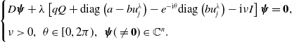 \begin{equation} \begin{cases} \displaystyle D \boldsymbol{\psi }+ \lambda \left [ q Q +\mathrm{diag}\left (a- b u_{j}^\lambda \right )- e^{-\textrm{i}\theta }\mathrm{diag}\left (b u_{j}^\lambda \right )-\textrm{i}\nu I\right ]\boldsymbol{\psi }=\textbf{0},\\[5pt] \nu \gt 0,\;\;\theta \in [0,2\pi ),\;\;\boldsymbol{\psi }(\neq \textbf{0}) \in \mathbb{C}^n. \end{cases} \end{equation}
By (2.17) and (2.18), we see that
 \begin{equation*} \mathbb {C}^n=\text {span}\{\boldsymbol {\varsigma }\}\oplus (\widetilde {X}_{1})_{\mathbb {C}}, \end{equation*}
where $\boldsymbol{\varsigma }$
and
$\boldsymbol{\varsigma }$
and $\widetilde{X}_1$
are defined in (2.17) and (2.18), respectively. Ignoring a scalar factor,
$\widetilde{X}_1$
are defined in (2.17) and (2.18), respectively. Ignoring a scalar factor, $\boldsymbol{\psi } (\neq \textbf{0}) \in \mathbb{C}^n$
in (3.40) can be represented as follows:
$\boldsymbol{\psi } (\neq \textbf{0}) \in \mathbb{C}^n$
in (3.40) can be represented as follows:
 \begin{equation} \begin{cases} \boldsymbol{\psi }=\gamma \boldsymbol{\varsigma }+{\boldsymbol{z}},\;\;{\boldsymbol{z}}\in (\widetilde{X}_{1})_{\mathbb{C}},\;\;\gamma \geq 0, \\[5pt] \|\boldsymbol{\psi }\|^{2}_{2}=\gamma ^2\|\boldsymbol{\varsigma }\|^{2}_{2}+\|{\boldsymbol{z}}\|^{2}_{2}=\|\boldsymbol{\varsigma }\|^{2}_{2}. \end{cases} \end{equation}
Then we obtain the equivalent problem of (3.40) in the following.
Lemma 3.10.
Assume that $\lambda \in (0,\lambda ^*_q)$
and
$\lambda \in (0,\lambda ^*_q)$
and $q\in (0,na)$
. Then
$q\in (0,na)$
. Then $(\boldsymbol{\psi },\nu, \theta )$
solves
(3.40), where
$(\boldsymbol{\psi },\nu, \theta )$
solves
(3.40), where $ \boldsymbol{\psi }$
is defined in
(3.41), if and only if
$ \boldsymbol{\psi }$
is defined in
(3.41), if and only if $(\gamma, \nu, \theta, {{\boldsymbol{z}}})$
solves
$(\gamma, \nu, \theta, {{\boldsymbol{z}}})$
solves
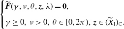 \begin{equation} \begin{cases} \widetilde{{{\boldsymbol{F}}}}(\gamma, \nu, \theta, {{\boldsymbol{z}}},\lambda )= \textbf{0},\\[5pt] \gamma \ge 0,\;\nu \gt 0,\;\theta \in [0,2\pi ),\;{{\boldsymbol{z}}}\in (\widetilde{X}_{1})_{\mathbb{C}}. \end{cases} \end{equation}
Here
 \begin{equation*} \widetilde {{{\boldsymbol{F}}}}(\gamma, \nu, \theta, {{\boldsymbol{z}}},\lambda )=( \widetilde {F}_{1,1},\cdots, \widetilde {F}_{1,n},\widetilde {F}_2,\widetilde {F}_3)^T\end{equation*}
is a continuously differentiable mapping from $\mathbb{R}^3\times (\widetilde{X}_{1})_{\mathbb{C}}\times \left [0,\lambda ^*_q\right )$
to
$\mathbb{R}^3\times (\widetilde{X}_{1})_{\mathbb{C}}\times \left [0,\lambda ^*_q\right )$
to $ (\widetilde{X}_{1})_{\mathbb{C}}\times \mathbb{C}\times \mathbb{R}$
, and
$ (\widetilde{X}_{1})_{\mathbb{C}}\times \mathbb{C}\times \mathbb{R}$
, and
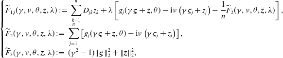 \begin{equation} \begin{cases} \displaystyle \widetilde{F}_{1,j}(\gamma, \nu, \theta, {{\boldsymbol{z}}},\lambda )\;:\!=\;\sum _{k=1}^nD_{jk}z_k+\lambda \left [g_j(\gamma \boldsymbol{\varsigma }+{{\boldsymbol{z}}},\theta )-\textrm{i}\nu \left (\gamma \varsigma _j+ z_j\right )-\frac{1}{n}\widetilde{F}_2(\gamma, \nu, \theta, {{\boldsymbol{z}}},\lambda )\right ],\\[5pt] \displaystyle \widetilde{F}_2(\gamma, \nu, \theta, {{\boldsymbol{z}}},\lambda )\;:\!=\;\sum _{j=1}^n\left [g_j(\gamma \boldsymbol{\varsigma }+{{\boldsymbol{z}}},\theta )-\textrm{i}\nu \left (\gamma \varsigma _j+ z_j\right )\right ],\\[5pt] \displaystyle \widetilde{F}_3(\gamma, \nu, \theta, {{\boldsymbol{z}}},\lambda )\;:\!=\;(\gamma ^2-1)\|\boldsymbol{\varsigma }\|_2^2+ \|{{\boldsymbol{z}}}\|_2^2, \end{cases} \end{equation}
where
 \begin{equation*} g_j(\gamma \boldsymbol {\varsigma }+{{\boldsymbol{z}}},\theta )=q\sum _{k=1}^n Q_{jk}\left (\gamma \varsigma _k+ z_k\right )+(a-bu^\lambda _j)\left (\gamma \varsigma _j+ z_j\right )- e^{-\textrm {i}\theta }bu^\lambda _j\left (\gamma \varsigma _j+ z_j\right ). \end{equation*}
Proof. Plugging (3.41) into (3.40), we see that
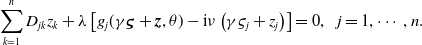 \begin{equation} \sum _{k=1}^nD_{jk}z_k+\lambda \left [g_j(\gamma \boldsymbol{\varsigma }+{{\boldsymbol{z}}},\theta )-\textrm{i}\nu \left (\gamma \varsigma _j+ z_j\right )\right ]=0,\;\;\;j=1,\cdots, n. \end{equation}
Denote the left side of (3.44) by $\tilde y_j$
and let
$\tilde y_j$
and let $\tilde{{{\boldsymbol{y}}}}=(\tilde y_1,\cdots, \tilde y_n)^T$
. Using similar arguments as in the proof of Proposition 2.5 (ii), we see that
$\tilde{{{\boldsymbol{y}}}}=(\tilde y_1,\cdots, \tilde y_n)^T$
. Using similar arguments as in the proof of Proposition 2.5 (ii), we see that $\tilde{{{\boldsymbol{y}}}}=\textbf{0}$
if and only
$\tilde{{{\boldsymbol{y}}}}=\textbf{0}$
if and only $\widetilde F_2=0$
and
$\widetilde F_2=0$
and $ \widetilde F_{1,j}=0$
for all
$ \widetilde F_{1,j}=0$
for all $j=1,\cdots, n$
. This completes the proof.
$j=1,\cdots, n$
. This completes the proof.
We first solve the equivalent problem $\widetilde{{\boldsymbol{F}}}(\gamma, \nu, \theta, {{\boldsymbol{z}}},\lambda )=\textbf{0}$
for
$\widetilde{{\boldsymbol{F}}}(\gamma, \nu, \theta, {{\boldsymbol{z}}},\lambda )=\textbf{0}$
for $\lambda =0$
.
$\lambda =0$
.
Lemma 3.11. The following equation
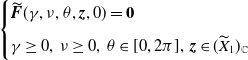 \begin{equation*} \begin{cases} \widetilde{{{\boldsymbol{F}}}}(\gamma, \nu, \theta, {{{\boldsymbol{z}}}},0)=\textbf{0} \\[5pt] \gamma \ge 0,\;\nu \ge 0,\;\theta \in [0,2\pi ],\;{{\boldsymbol{z}}}\in (\widetilde{X}_{1})_{\mathbb{C}} \end{cases} \end{equation*}
has a unique solution $\left (\gamma _*, \nu _*,\theta _*,{{\boldsymbol{z}}}_*\right )$
, where
$\left (\gamma _*, \nu _*,\theta _*,{{\boldsymbol{z}}}_*\right )$
, where
 \begin{equation*}{{\boldsymbol{z}}}_*=\textbf{0},\;\; \gamma _*=1,\;\;\nu _*=a-\frac {q}{n},\;\;\theta _*=\frac {\pi }{2}. \end{equation*}
Proof. Clearly,
 \begin{equation*}\left (\widetilde {F}_{1,1}(\gamma, \nu, \theta, {{{\boldsymbol{z}}}},0),\cdots, \widetilde {F}_{1,n}(\gamma, \nu, \theta, {{{\boldsymbol{z}}}},0)\right )=\textbf{0},\end{equation*}
if and only if ${{\boldsymbol{z}}}={{\boldsymbol{z}}}_*=\textbf{0}$
. Plugging
${{\boldsymbol{z}}}={{\boldsymbol{z}}}_*=\textbf{0}$
. Plugging ${{\boldsymbol{z}}}=\textbf{0}$
into
${{\boldsymbol{z}}}=\textbf{0}$
into $\widetilde{F}_3(\gamma, \nu, \theta, {{{\boldsymbol{z}}}},0)= 0$
, we have
$\widetilde{F}_3(\gamma, \nu, \theta, {{{\boldsymbol{z}}}},0)= 0$
, we have $\gamma =\gamma _*=1$
. Note from Proposition 2.6 that
$\gamma =\gamma _*=1$
. Note from Proposition 2.6 that $\displaystyle u^0_{j}=\frac{na-q}{nb}$
for
$\displaystyle u^0_{j}=\frac{na-q}{nb}$
for $j=1,\cdots, n$
. Then plugging
$j=1,\cdots, n$
. Then plugging ${{\boldsymbol{z}}}=\textbf{0}$
and
${{\boldsymbol{z}}}=\textbf{0}$
and $\gamma =1$
into
$\gamma =1$
into $\widetilde{F}_2(\gamma, \nu, \theta, {{{\boldsymbol{z}}}},0)= 0$
, we have
$\widetilde{F}_2(\gamma, \nu, \theta, {{{\boldsymbol{z}}}},0)= 0$
, we have
 \begin{equation*} \sum _{j=1}^n\left [q\sum _{k=1}^nQ_{jk}\varsigma _k+\displaystyle \frac {q}{n}\varsigma _j-e^{-\textrm {i}\theta }\varsigma _j\displaystyle \frac {na-q}{n}\right ]-\textrm {i}\nu =0, \end{equation*}
which yields
 \begin{equation*}\nu =\nu _*=a-\frac {q}{n}, \;\;\theta =\theta _*=\frac {\pi }{2}.\end{equation*}
This completes the proof.
Now we solve $\widetilde{{{\boldsymbol{F}}}}(\gamma, \nu, \theta, {\boldsymbol{z}},\lambda )=\textbf{0}$
for
$\widetilde{{{\boldsymbol{F}}}}(\gamma, \nu, \theta, {\boldsymbol{z}},\lambda )=\textbf{0}$
for $0\lt \lambda \ll 1$
.
$0\lt \lambda \ll 1$
.
Lemma 3.12.
There exists $\tilde \lambda$
with
$\tilde \lambda$
with $0\lt \tilde \lambda \ll 1$
and a continuously differentiable mapping
$0\lt \tilde \lambda \ll 1$
and a continuously differentiable mapping $\lambda \mapsto \left (\gamma ^\lambda, \nu ^\lambda, \theta ^\lambda, {{\boldsymbol{z}}}^\lambda \right )$
from
$\lambda \mapsto \left (\gamma ^\lambda, \nu ^\lambda, \theta ^\lambda, {{\boldsymbol{z}}}^\lambda \right )$
from $[0,\tilde \lambda ]$
to
$[0,\tilde \lambda ]$
to $\mathbb{R}^{3}\times (\widetilde{X}_{1})_{\mathbb{C}}$
such that
$\mathbb{R}^{3}\times (\widetilde{X}_{1})_{\mathbb{C}}$
such that $(\gamma ^\lambda, \nu ^\lambda, \theta ^\lambda, {{\boldsymbol{z}}}^\lambda )$
is the unique solution of the following problem:
$(\gamma ^\lambda, \nu ^\lambda, \theta ^\lambda, {{\boldsymbol{z}}}^\lambda )$
is the unique solution of the following problem:
 \begin{equation} \begin{cases} \widetilde{{{\boldsymbol{F}}}}\left (\gamma, \nu, \theta, {{{\boldsymbol{z}}}},\lambda \right )=\textbf{0} \\[5pt] \gamma \ge 0,\;\nu \gt 0,\;\theta \in [0,2\pi ),\;{{\boldsymbol{z}}}\in (\widetilde{X}_{1})_{\mathbb{C}} \end{cases} \end{equation}
for $\lambda \in [0,\tilde \lambda ]$
.
$\lambda \in [0,\tilde \lambda ]$
.
Proof. Let $\widetilde{{{\boldsymbol{P}}}}\left (\check{\gamma },\check{\nu },\check{\theta },\check{{{{\boldsymbol{z}}}}}\right )=\left (\widetilde{P}_{1,1}, \cdots, \widetilde{P}_{1,n},\widetilde{P}_2,\widetilde{P}_3\right )^T \;:\; \mathbb{R}^3 \times (\widetilde{X}_{1})_{\mathbb{C}} \to (\widetilde{X}_{1})_{\mathbb{C}}\times \mathbb{C}\times \mathbb{R}$
be the Fréchet derivative of
$\widetilde{{{\boldsymbol{P}}}}\left (\check{\gamma },\check{\nu },\check{\theta },\check{{{{\boldsymbol{z}}}}}\right )=\left (\widetilde{P}_{1,1}, \cdots, \widetilde{P}_{1,n},\widetilde{P}_2,\widetilde{P}_3\right )^T \;:\; \mathbb{R}^3 \times (\widetilde{X}_{1})_{\mathbb{C}} \to (\widetilde{X}_{1})_{\mathbb{C}}\times \mathbb{C}\times \mathbb{R}$
be the Fréchet derivative of $\widetilde{{{\boldsymbol{F}}}}$
with respect to
$\widetilde{{{\boldsymbol{F}}}}$
with respect to $(\gamma, \nu, \theta, {{{\boldsymbol{z}}}})$
at
$(\gamma, \nu, \theta, {{{\boldsymbol{z}}}})$
at $\left (\gamma _*, \nu _*,\theta _*,{{\boldsymbol{z}}}_*,0\right )$
. Then we compute that
$\left (\gamma _*, \nu _*,\theta _*,{{\boldsymbol{z}}}_*,0\right )$
. Then we compute that
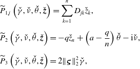 \begin{equation*} \begin{split} &\widetilde{P}_{1,j}\left (\check{\gamma },\check{\nu },\check{\theta },\check{{{{\boldsymbol{z}}}}}\right )=\sum _{k=1}^{n}D_{jk} \check{z}_{k},\\[5pt] &\widetilde{P}_{2}\left (\check{\gamma },\check{\nu },\check{\theta },\check{{{{\boldsymbol{z}}}}}\right )=-q\check{z}_n+\left (a-\frac{q}{n}\right )\check{\theta } - \mathrm{i}\check{\nu },\\[5pt] &\widetilde{P}_{3}\left (\check{\gamma },\check{\nu },\check{\theta },\check{{{{\boldsymbol{z}}}}}\right )=2\|\boldsymbol{\varsigma }\|^2_2\check{\gamma }, \end{split} \end{equation*}
where we have used $\sum _{j=1}^n \check z_j=0$
to obtain
$\sum _{j=1}^n \check z_j=0$
to obtain $\widetilde P_2$
. Clearly,
$\widetilde P_2$
. Clearly, $\widetilde{{{\boldsymbol{P}}}}$
is a bijection from
$\widetilde{{{\boldsymbol{P}}}}$
is a bijection from $\mathbb{R}^3 \times (\widetilde{X}_{1})_{\mathbb{C}}$
to
$\mathbb{R}^3 \times (\widetilde{X}_{1})_{\mathbb{C}}$
to $\mathbb{R}\times \mathbb{C} \times (\widetilde{X}_{1})_{\mathbb{C}}$
. It follows from the implicit function theorem that there exists
$\mathbb{R}\times \mathbb{C} \times (\widetilde{X}_{1})_{\mathbb{C}}$
. It follows from the implicit function theorem that there exists $\tilde \lambda \gt 0$
with
$\tilde \lambda \gt 0$
with $0\lt \tilde \lambda \ll 1$
and a continuously differentiable mapping
$0\lt \tilde \lambda \ll 1$
and a continuously differentiable mapping $\lambda \mapsto \left (\gamma ^\lambda, \nu ^\lambda, \theta ^\lambda, {{\boldsymbol{z}}}^\lambda \right )$
from
$\lambda \mapsto \left (\gamma ^\lambda, \nu ^\lambda, \theta ^\lambda, {{\boldsymbol{z}}}^\lambda \right )$
from $[0,\tilde \lambda ]$
to
$[0,\tilde \lambda ]$
to $\mathbb{R}^3 \times (\widetilde{X}_{1})_{\mathbb{C}}$
such that
$\mathbb{R}^3 \times (\widetilde{X}_{1})_{\mathbb{C}}$
such that $\left (\gamma ^\lambda, \nu ^\lambda, \theta ^\lambda, {{\boldsymbol{z}}}^\lambda \right )$
satisfies (3.45).
$\left (\gamma ^\lambda, \nu ^\lambda, \theta ^\lambda, {{\boldsymbol{z}}}^\lambda \right )$
satisfies (3.45).
Then we prove the uniqueness of the solution of (3.45). Actually, we only need to verify that if $\left (\gamma _\lambda, \nu _\lambda, \theta _\lambda, {{\boldsymbol{z}}}_\lambda \right )$
satisfies (3.45), then
$\left (\gamma _\lambda, \nu _\lambda, \theta _\lambda, {{\boldsymbol{z}}}_\lambda \right )$
satisfies (3.45), then $\displaystyle \lim _{\lambda \to 0}\left (\gamma _\lambda, \nu _\lambda, \theta _\lambda, {{\boldsymbol{z}}}_\lambda \right )=\left (\gamma _*, \nu _*,\theta _*,{{\boldsymbol{z}}}_*\right )$
. Since
$\displaystyle \lim _{\lambda \to 0}\left (\gamma _\lambda, \nu _\lambda, \theta _\lambda, {{\boldsymbol{z}}}_\lambda \right )=\left (\gamma _*, \nu _*,\theta _*,{{\boldsymbol{z}}}_*\right )$
. Since $\widetilde F_3\left (\gamma _\lambda, \nu _\lambda, \theta _\lambda, {{\boldsymbol{z}}}_\lambda, \lambda \right )=0$
, we see that
$\widetilde F_3\left (\gamma _\lambda, \nu _\lambda, \theta _\lambda, {{\boldsymbol{z}}}_\lambda, \lambda \right )=0$
, we see that
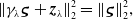 \begin{equation} \| \gamma _\lambda \boldsymbol{\varsigma }+{{\boldsymbol{z}}}_\lambda \|_2^{2}=\|\boldsymbol{\varsigma }\|_2^2, \end{equation}
which implies that $\gamma _\lambda$
is bounded for
$\gamma _\lambda$
is bounded for $\lambda \in (0,\tilde \lambda )$
. Note from Lemma 3.1 (iii) that
$\lambda \in (0,\tilde \lambda )$
. Note from Lemma 3.1 (iii) that $\nu _\lambda$
is bounded for
$\nu _\lambda$
is bounded for $\lambda \in (0,\tilde \lambda ]$
. This combined with (3.46) and the first equation of (3.43) implies that
$\lambda \in (0,\tilde \lambda ]$
. This combined with (3.46) and the first equation of (3.43) implies that $\displaystyle \lim _{\lambda \to 0}D{{\boldsymbol{z}}}_\lambda =\textbf{0}$
, and consequently,
$\displaystyle \lim _{\lambda \to 0}D{{\boldsymbol{z}}}_\lambda =\textbf{0}$
, and consequently, $\displaystyle \lim _{\lambda \to 0}{{\boldsymbol{z}}}_\lambda =\textbf{0}$
. By the third equation of (3.43), we obtain that
$\displaystyle \lim _{\lambda \to 0}{{\boldsymbol{z}}}_\lambda =\textbf{0}$
. By the third equation of (3.43), we obtain that $\displaystyle \lim _{\lambda \to 0}\gamma _\lambda =1$
. Then, it follows the second equation of (3.43) that
$\displaystyle \lim _{\lambda \to 0}\gamma _\lambda =1$
. Then, it follows the second equation of (3.43) that $\displaystyle \lim _{\lambda \to 0}\theta _\lambda =\theta _*$
and
$\displaystyle \lim _{\lambda \to 0}\theta _\lambda =\theta _*$
and $\displaystyle \lim _{\lambda \to 0}\nu _\lambda =\nu _*$
. Therefore,
$\displaystyle \lim _{\lambda \to 0}\nu _\lambda =\nu _*$
. Therefore, $\left (\beta _\lambda, \nu _\lambda, \theta _\lambda, {{\boldsymbol{z}}}_\lambda \right )\rightarrow \left (\gamma _*, \nu _*,\theta _*,{{\boldsymbol{z}}}_*\right )$
as
$\left (\beta _\lambda, \nu _\lambda, \theta _\lambda, {{\boldsymbol{z}}}_\lambda \right )\rightarrow \left (\gamma _*, \nu _*,\theta _*,{{\boldsymbol{z}}}_*\right )$
as $\lambda \rightarrow 0$
. This completes the proof.
$\lambda \rightarrow 0$
. This completes the proof.
By Lemma 3.12, we obtain the following result.
Theorem 3.13.
Assume that $q\in (0,na)$
and let
$q\in (0,na)$
and let $\lambda =1/d$
. Then for
$\lambda =1/d$
. Then for $d\in \left [\tilde d_3,\infty \right )$
with
$d\in \left [\tilde d_3,\infty \right )$
with $\tilde d_3\gg 1$
,
$\tilde d_3\gg 1$
, $\left (\nu, \tau, \boldsymbol{\psi }\right )$
satisfies
(3.18) if and only if
$\left (\nu, \tau, \boldsymbol{\psi }\right )$
satisfies
(3.18) if and only if
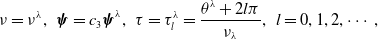 \begin{equation*} \nu =\nu ^\lambda, \;\;\boldsymbol \psi =c_3 \boldsymbol \psi ^\lambda, \;\;\tau =\tau ^\lambda _{l}=\frac {\theta ^\lambda +2l\pi }{\nu _\lambda },\;\;l=0,1,2,\cdots, \end{equation*}
where $\boldsymbol \psi ^\lambda =\gamma ^\lambda \boldsymbol \varsigma +{{\boldsymbol{z}}}^\lambda$
,
$\boldsymbol \psi ^\lambda =\gamma ^\lambda \boldsymbol \varsigma +{{\boldsymbol{z}}}^\lambda$
, $c_3\in \mathbb{C}$
is a non-zero constant, and
$c_3\in \mathbb{C}$
is a non-zero constant, and $\left (\gamma ^\lambda, \nu ^\lambda, \theta ^\lambda, {{\boldsymbol{z}}}^\lambda \right )$
is defined in Lemma 3.12
.
$\left (\gamma ^\lambda, \nu ^\lambda, \theta ^\lambda, {{\boldsymbol{z}}}^\lambda \right )$
is defined in Lemma 3.12
.
4. Local dynamics
In this section, we obtain the local dynamics of model (1.5) and show the existence of Hopf bifurcations. We first show that the purely imaginary eigenvalues obtained in Theorems 3.5, 3.9 and 3.13 are simple.
Lemma 4.1.
Let $\lambda =1/d$
, and define
$\lambda =1/d$
, and define
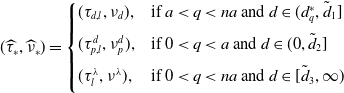 \begin{equation*} (\widehat \tau _*,\widehat \nu _*)=\begin {cases} (\tau _{d,l},\nu _d),&\text {if } a\lt q\lt na \text { and } d\in (d_q^*,\tilde d_1]\\[5pt] (\tau _{p,l}^d,\nu _p^d),&\text {if } 0\lt q\lt a \text { and } d\in (0,\tilde d_2]\\[5pt] (\tau ^\lambda _l,\nu ^\lambda ),&\text {if } 0\lt q\lt na \text { and } d\in [\tilde d_3,\infty )\\[5pt] \end {cases} \end{equation*}
with $p=1,\cdots, n$
and
$p=1,\cdots, n$
and $l=1,2,\cdots$
, where
$l=1,2,\cdots$
, where $(\tau _{d,l},\nu _d,\tilde d_1)$
,
$(\tau _{d,l},\nu _d,\tilde d_1)$
, $(\tau _{p,l}^d,\nu _p^d,\tilde d_2)$
and
$(\tau _{p,l}^d,\nu _p^d,\tilde d_2)$
and $(\tau ^\lambda _l,\nu ^\lambda, \tilde d_3)$
are defined in Theorems
3.5,
3.9 and
3.13, respectively. Then,
$(\tau ^\lambda _l,\nu ^\lambda, \tilde d_3)$
are defined in Theorems
3.5,
3.9 and
3.13, respectively. Then, $\mu =\rm{i}\widehat \nu _*$
is an algebraically simple eigenvalue of
$\mu =\rm{i}\widehat \nu _*$
is an algebraically simple eigenvalue of $A_{\widehat \tau _{*}}(d)$
.
$A_{\widehat \tau _{*}}(d)$
.
Proof. For simplicity, we only consider the case that $0\lt q\lt a$
and
$0\lt q\lt a$
and $d\in (0,\tilde d_2]$
, and other cases can be proved similarly. For this case,
$d\in (0,\tilde d_2]$
, and other cases can be proved similarly. For this case, $\widehat \tau _*=\tau ^d_{p,l}$
and
$\widehat \tau _*=\tau ^d_{p,l}$
and $\widehat \nu _*=\nu ^d_p$
with
$\widehat \nu _*=\nu ^d_p$
with $l=0,1,\cdots$
and
$l=0,1,\cdots$
and $p=1,\cdots, n$
. It from Theorem 3.9 that
$p=1,\cdots, n$
. It from Theorem 3.9 that $\mathscr{N}\left [A_{\tau ^d_{p,l}}(d)-\textrm{i} \nu ^d_p\right ]=\textrm{span}\left [e^{\textrm{i} \nu ^d_p \theta }\boldsymbol{\psi }_p^d\right ]$
, where
$\mathscr{N}\left [A_{\tau ^d_{p,l}}(d)-\textrm{i} \nu ^d_p\right ]=\textrm{span}\left [e^{\textrm{i} \nu ^d_p \theta }\boldsymbol{\psi }_p^d\right ]$
, where $\theta \in [- \tau ^d_{p,l},0]$
and
$\theta \in [- \tau ^d_{p,l},0]$
and $\boldsymbol{\psi }^d_p$
is defined in Theorem 3.9. Now we show that
$\boldsymbol{\psi }^d_p$
is defined in Theorem 3.9. Now we show that
 \begin{equation*}\mathscr {N}\left [A_{\tau ^d_{p,l}}(d)-\textrm {i} \nu ^d_p\right ]^{2}=\mathscr {N}\left [A_{\tau ^d_{p,l}}(d)-\textrm {i} \nu ^d_p\right ].\end{equation*}
If $\boldsymbol{\phi } \in \mathscr{N}\left [A_{\tau ^d_{p,l}}(d)-\textrm{i} \nu ^d_p\right ]^2$
, then
$\boldsymbol{\phi } \in \mathscr{N}\left [A_{\tau ^d_{p,l}}(d)-\textrm{i} \nu ^d_p\right ]^2$
, then
 \begin{equation*} \left [A_{\tau ^d_{p,l}}(d)-\textrm {i} \nu ^d_p\right ]\boldsymbol {\phi } \in \mathscr {N}\left [A_{\tau ^d_{p,l}}(d)-\textrm {i} \nu ^d_p\right ]=\textrm {span}\left [e^{\textrm {i} \nu ^d_p\theta }\boldsymbol {\psi }^d_p\right ], \end{equation*}
and consequently, there is a constant $\sigma$
such that
$\sigma$
such that
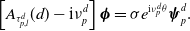 \begin{equation*} \left [A_{\tau ^d_{p,l}}(d)-\textrm {i} \nu ^d_p\right ]\boldsymbol {\phi }=\sigma e^{\textrm {i} \nu ^d_p \theta }\boldsymbol {\psi }^d_p. \end{equation*}
This together with (3.2) and (3.3) yields
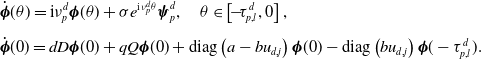 \begin{equation} \begin{split} &\dot{\boldsymbol{\phi }}(\theta ) =\textrm{i} \nu ^d_p\boldsymbol{\phi }(\theta )+\sigma e^{\textrm{i}\nu ^d_p \theta }\boldsymbol{\psi }^d_p, \quad \theta \in \left [\!-\!\tau ^d_{p,l}, 0\right ], \\[5pt] &\dot{\boldsymbol{\phi }}(0)=dD \boldsymbol{\phi }(0)+ qQ\boldsymbol{\phi }(0)+\textrm{diag}\left (a- bu_{d,j}\right )\boldsymbol{\phi }(0)-\textrm{diag}\left (bu_{d,j}\right )\boldsymbol{\phi }(-\tau ^d_{p,l}). \end{split} \end{equation}
By the first equation of (4.1), we have
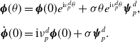 \begin{equation} \begin{split} \boldsymbol{\phi }(\theta ) &=\boldsymbol{\phi }(0) e^{\textrm{i} \nu ^d_p \theta }+\sigma \theta e^{\textrm{i} \nu ^d_p\theta }\boldsymbol{\psi }^d_p, \\[5pt] \dot{\boldsymbol{\phi }}(0) &=\textrm{i} \nu ^d_p\boldsymbol{\phi }(0)+\sigma \boldsymbol{\psi }^d_p. \end{split} \end{equation}
Note from Theorem 3.9 that $e^{-\textrm{i}\tau ^d_{p,l}\nu ^d_p}=e^{-\textrm{i}\theta ^d_p}$
with
$e^{-\textrm{i}\tau ^d_{p,l}\nu ^d_p}=e^{-\textrm{i}\theta ^d_p}$
with $\theta ^d_p$
defined in Lemma 3.8. Then, substituting (4.2) into the second equation of (4.1), we have
$\theta ^d_p$
defined in Lemma 3.8. Then, substituting (4.2) into the second equation of (4.1), we have
 \begin{equation} \mathcal M\left (d,\theta ^d_p,\nu ^d_p\right )\boldsymbol \phi (0)\\[5pt] = \sigma \left (\boldsymbol \psi ^d_p- \tau ^d_{p,l} e^{{-\textrm{i}} \theta ^d_p}\textrm{diag}\left (bu_{d,j}\right )\boldsymbol{\psi }^d_p\right ), \end{equation}
where $\mathcal M(d,\nu, \theta )$
is defined in (3.6).
$\mathcal M(d,\nu, \theta )$
is defined in (3.6).
Let $\mathcal M^H(d,\nu, \theta )$
be the conjugate transpose of
$\mathcal M^H(d,\nu, \theta )$
be the conjugate transpose of $\mathcal M(d,\nu, \theta )$
. Using similar arguments as in the proof of Lemma 3.8, we obtain that for
$\mathcal M(d,\nu, \theta )$
. Using similar arguments as in the proof of Lemma 3.8, we obtain that for $d\in (0,\tilde d_2]$
,
$d\in (0,\tilde d_2]$
,
 \begin{equation*} \left \{\boldsymbol {\varphi }\in \mathbb {C}^n\;:\;\mathcal M^H(d,\nu ^d_p,\theta ^d_p)\boldsymbol {\varphi }=\textbf{0}\right \}=\{c{\boldsymbol \varphi }_p^d\;:\;c\in \mathbb {C}\}, \end{equation*}
and $\displaystyle \lim _{d\to 0}{\boldsymbol \varphi }_p^d={\boldsymbol \varphi }_p^0$
. Here,
$\displaystyle \lim _{d\to 0}{\boldsymbol \varphi }_p^d={\boldsymbol \varphi }_p^0$
. Here, ${\boldsymbol \varphi }_p^0=\left ({\varphi }_{p,1}^0,\cdots, \varphi _{p,n}^0\right )^T$
satisfies
${\boldsymbol \varphi }_p^0=\left ({\varphi }_{p,1}^0,\cdots, \varphi _{p,n}^0\right )^T$
satisfies
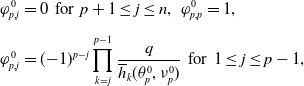 \begin{equation*} \begin{split} &\varphi ^{0}_{p,j}=0\;\;\text{for}\;\;p+1\le j\le n,\;\;\varphi ^{0}_{p,p}=1,\\[5pt] &\varphi ^{0}_{p,j}=(\!-\!1)^{p-j}\prod ^{p-1}_{k=j}\frac{q}{{\overline h}_{k}(\theta ^{0}_{p},\nu ^0_{p})}\;\;\text{for}\;\;1\le j\le p-1, \end{split} \end{equation*}
where $\overline{{h}}_k\left (\theta ^0_p,\nu ^0_p\right )$
is the conjugate of
$\overline{{h}}_k\left (\theta ^0_p,\nu ^0_p\right )$
is the conjugate of ${h}_k\left (\theta ^0_p,\nu ^0_p\right )$
, and
${h}_k\left (\theta ^0_p,\nu ^0_p\right )$
, and $h_k(\theta, \nu )$
is defined in (3.23). One can also refer to (3.30) for
$h_k(\theta, \nu )$
is defined in (3.23). One can also refer to (3.30) for $p=2$
. Then by (4.3), we have
$p=2$
. Then by (4.3), we have
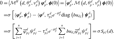 \begin{equation*} \begin{split} 0=&\left \langle \mathcal M^H\left (d,\theta ^d_p,\nu ^d_p\right )\boldsymbol{\varphi }^d_p,\boldsymbol \phi (0)\right \rangle =\left \langle \boldsymbol{\varphi }^d_p,\mathcal M\left (d,\theta ^d_p,\nu ^d_p\right )\boldsymbol \phi (0)\right \rangle \\[5pt] =&\sigma \left [{\langle \boldsymbol{\varphi }^d_p,\boldsymbol{\psi }^d_p \rangle }-{\langle \boldsymbol{\varphi }^d, \tau ^d_{p,l} e^{{-\textrm{i}} \theta ^d_p}\textrm{diag}\left (bu_{d,j}\right )\boldsymbol{\psi }^d_p\rangle }\right ]\\[5pt] =&\sigma \left [\sum _{j=1}^n \overline{\varphi }^d_{p,j}\psi ^d_{p,j}- \tau ^d_{p,l} e^{{-\textrm{i}} \theta ^d_p}\sum _{j=1}^n bu_{d,j}\overline{\varphi }^d_{p,j}\psi ^d_{p,j}\right ] =\sigma S_{p,l}(d). \end{split} \end{equation*}
where
 \begin{equation*} S_{p,l}(d)\;:\!=\;\sum _{j=1}^n \overline {\varphi }^d_{p,j}\psi ^d_{p,j}- \tau ^d_{p,l} e^{{-\textrm {i}} \theta ^d_p}\sum _{j=1}^n bu_{d,j}\overline {\varphi }^d_{p,j}\psi ^d_{p,j}\;\;\text {for}\;\;p=1,\cdots, n\;\;\text {and}\;\;l=0,1,\cdots . \end{equation*}
By Lemmas 3.6, 3.8 and Theorem 3.9, we obtain that
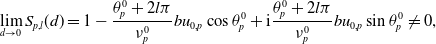 \begin{equation*} \begin{aligned} \lim _{d \rightarrow 0} S_{p,l}(d) &=1-\frac{\theta ^0_p+2l\pi }{\nu ^0_p}bu_{0,p}\cos \theta ^0_p+\mathrm{i}\frac{\theta ^0_p+2l\pi }{\nu ^0_p} bu_{0,p}\sin \theta ^0_p\neq 0, \end{aligned} \end{equation*}
which implies $\sigma = 0$
. Therefore, for any
$\sigma = 0$
. Therefore, for any $l=1,2,\cdots$
,
$l=1,2,\cdots$
,
 \begin{equation*}\mathscr {N}\left [A_{\tau ^d_{p,l}}(d)-\textrm {i} \nu ^d_p\right ]^{2}=\mathscr {N}\left [{A}_{\tau ^d_{p,l}}(d)-\textrm {i} \nu ^d_p\right ],\end{equation*}
and consequently, $\textrm{i} \nu ^d_p$
is a simple eigenvalue of
$\textrm{i} \nu ^d_p$
is a simple eigenvalue of $A_{\tau ^d_{p,l}}$
for
$A_{\tau ^d_{p,l}}$
for $l=0,1,2, \cdots$
.
$l=0,1,2, \cdots$
.
It follows from Lemma 4.1 that $\mu =\textrm{i} \widehat \nu _*$
is an algebraically simple eigenvalue of
$\mu =\textrm{i} \widehat \nu _*$
is an algebraically simple eigenvalue of $A_{\widehat \tau _*}$
. Then, by the implicit function theorem, we see that there exists a neighbourhood
$A_{\widehat \tau _*}$
. Then, by the implicit function theorem, we see that there exists a neighbourhood $\widehat{O}_{*} \times \widehat{D}_{*} \times \widehat{H}_{*}$
of
$\widehat{O}_{*} \times \widehat{D}_{*} \times \widehat{H}_{*}$
of $\left (\widehat \tau _*,\textrm{i} \widehat \nu _*, \widehat{\boldsymbol \psi }_*\right )$
and a continuously differentiable function
$\left (\widehat \tau _*,\textrm{i} \widehat \nu _*, \widehat{\boldsymbol \psi }_*\right )$
and a continuously differentiable function $\left (\mu (\tau ), \boldsymbol{\psi }(\tau )\right ) \;:\; \widehat{O}_{*} \rightarrow \widehat{D}_{*} \times \widehat{H}_{*}$
such that
$\left (\mu (\tau ), \boldsymbol{\psi }(\tau )\right ) \;:\; \widehat{O}_{*} \rightarrow \widehat{D}_{*} \times \widehat{H}_{*}$
such that $\mu (\widehat \tau _*)=\textrm{i} \widehat \nu _*$
,
$\mu (\widehat \tau _*)=\textrm{i} \widehat \nu _*$
, $\boldsymbol{\psi }(\widehat \tau _*)=\widehat{\boldsymbol \psi }_*$
, and for
$\boldsymbol{\psi }(\widehat \tau _*)=\widehat{\boldsymbol \psi }_*$
, and for $\tau \in \widehat{O}_{*}$
,
$\tau \in \widehat{O}_{*}$
,
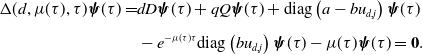 \begin{equation} \begin{aligned} \Delta (d, \mu (\tau ), \tau )\boldsymbol{\psi }(\tau ) =&dD\boldsymbol{\psi }(\tau )+ qQ\boldsymbol{\psi }(\tau )+ \textrm{diag}\left (a-bu_{d,j}\right )\boldsymbol{\psi }(\tau )\\[5pt] &- e^{-\mu (\tau ) \tau } \textrm{diag}\left (bu_{d,j}\right )\boldsymbol{\psi }(\tau )-\mu (\tau ) \boldsymbol{\psi }(\tau )=\textbf{0}. \end{aligned} \end{equation}
Here
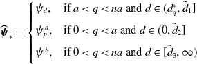 \begin{equation*} \widehat{\boldsymbol \psi }_*=\begin{cases} \psi _d,&\text{if } a\lt q\lt na \text{ and } d\in (d_q^*,\tilde d_1]\\[5pt] \psi _p^d,&\text{if } 0\lt q\lt a \text{ and } d\in (0,\tilde d_2]\\[5pt] \psi ^\lambda, &\text{if } 0\lt q\lt na \text{ and } d\in [\tilde d_3,\infty )\\[5pt] \end{cases} \end{equation*}
with $\lambda =1/d$
and
$\lambda =1/d$
and $p=1,\cdots, n$
, where
$p=1,\cdots, n$
, where $(\psi _d,\tilde d_1)$
,
$(\psi _d,\tilde d_1)$
, $(\psi _p^d,\tilde d_2)$
and
$(\psi _p^d,\tilde d_2)$
and $(\psi ^\lambda, \tilde d_3)$
are defined in Theorems 3.5, 3.9 and 3.13, respectively. By a direct calculation, we obtain the following transversality condition.
$(\psi ^\lambda, \tilde d_3)$
are defined in Theorems 3.5, 3.9 and 3.13, respectively. By a direct calculation, we obtain the following transversality condition.
Lemma 4.2.
Let $\widehat \tau _*$
be defined in Lemma 4.1
. Then
$\widehat \tau _*$
be defined in Lemma 4.1
. Then
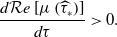 \begin{equation*} \frac {d \mathcal {R} e\left [\mu \left (\widehat \tau _*\right )\right ]}{d \tau }\gt 0. \end{equation*}
Proof. Similar to Lemma 4.1, we only consider the case that $0\lt q\lt a$
and
$0\lt q\lt a$
and $d\in (0,\tilde d_2]$
, and other cases can be proved similarly. For this case,
$d\in (0,\tilde d_2]$
, and other cases can be proved similarly. For this case, $\widehat \tau _*=\tau ^d_{p,l}$
,
$\widehat \tau _*=\tau ^d_{p,l}$
, $\widehat \nu _*=\nu ^d_p$
and
$\widehat \nu _*=\nu ^d_p$
and $\widehat{\boldsymbol \psi }_*=\boldsymbol \psi ^d_p$
with
$\widehat{\boldsymbol \psi }_*=\boldsymbol \psi ^d_p$
with $p=1,\cdots, n$
and
$p=1,\cdots, n$
and $l=0,1,\cdots$
. Differentiating (4.4) with respect to
$l=0,1,\cdots$
. Differentiating (4.4) with respect to $\tau$
at
$\tau$
at $\tau =\tau ^d_{p,l}$
, we have
$\tau =\tau ^d_{p,l}$
, we have
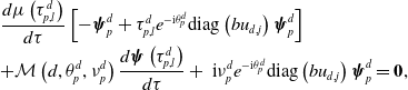 \begin{equation} \begin{array}{l} \displaystyle{\frac{d \mu \left (\tau ^d_{p,l}\right )}{d \tau }\left [-\boldsymbol{\psi }^d_p+ \tau ^d_{p,l}e^{-\textrm{i}\theta ^d_p}\textrm{diag}\left ( bu_{d,j}\right )\boldsymbol{\psi }^d_p \right ]} \\[5pt] \displaystyle{+\mathcal M\left (d,\theta ^d_p,\nu ^d_p\right ) \frac{d\boldsymbol{\psi } \left (\tau ^d_{p,l}\right )}{d \tau } + \textrm{ i} \nu ^d_p e^{-\textrm{i}\theta ^d_p} \textrm{diag}\left ( bu_{d,j}\right )\boldsymbol \psi ^d_p }=\textbf{0}, \end{array} \end{equation}
where $\mathcal M(d,\nu, \theta )$
is defined in (3.6). Note that, for
$\mathcal M(d,\nu, \theta )$
is defined in (3.6). Note that, for $l=0,1,\cdots$
,
$l=0,1,\cdots$
,
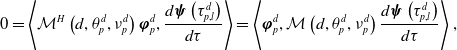 \begin{equation*} 0=\left \langle \mathcal M^H\left (d,\theta ^d_p,\nu ^d_p\right )\boldsymbol {\varphi }^d_p,\frac {d\boldsymbol {\psi }\left (\tau ^d_{p,l}\right ) }{d \tau }\right \rangle =\left \langle \boldsymbol {\varphi }^d_p,\mathcal M\left (d,\theta ^d_p,\nu ^d_p\right )\frac {d\boldsymbol {\psi } \left (\tau ^d_{p,l}\right )}{d \tau }\right \rangle, \end{equation*}
where $\mathcal M^H(d,\nu, \theta )$
and
$\mathcal M^H(d,\nu, \theta )$
and $\boldsymbol{\varphi }^d_p$
are defined in the proof of Lemma 4.1. This combined with (4.5) implies that
$\boldsymbol{\varphi }^d_p$
are defined in the proof of Lemma 4.1. This combined with (4.5) implies that
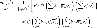 \begin{equation*} \begin{aligned} \frac{d \mu \left (\tau ^d_{p,l}\right )}{d \tau } =&\frac{1}{\left |S_{l}(d)\right |^{2}}\left [\mathrm{i} \nu ^d_p e^{-\mathrm{i}\theta ^d_p }\left ( \sum _{j=1}^{n}bu_{d,j}\overline{\varphi }^d_{p,j}\psi ^d_{p,j}\right )\left (\sum _{j=1}^{n}\varphi ^d_{p,j} \overline{\psi }^d_{p,j} \right )\right .\\[5pt] &\left .-\textrm{i}\nu ^d_p\tau ^d_{p,l}\left (\sum _{j=1}^{n} bu_{d,j}\varphi ^d_{p,j}\overline{\psi }^d_{p,j} \right )\left (\sum _{j=1}^{n} bu_{d,j}\overline{\varphi }^d_{p,j}\psi ^d_{p,j}\right )\right ]. \end{aligned} \end{equation*}
By Lemmas 3.6 and 3.8 and Theorem 3.9, we obtain that
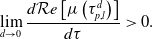 \begin{equation*} \lim _{d \rightarrow 0} \frac {d \mathcal {R} e\left [\mu \left (\tau ^d_{p,l}\right )\right ]}{d \tau }\gt 0. \end{equation*}
This completes the proof.
By Theorems 3.5, 3.9 and 3.13 and Lemmas 4.1 and 4.2, we obtain the following result.
Theorem 4.3.
Let ${\boldsymbol{u}}_d$
be the unique positive equilibrium of model
(1.5) obtained in Proposition 2.4
. Then the following statements hold:
${\boldsymbol{u}}_d$
be the unique positive equilibrium of model
(1.5) obtained in Proposition 2.4
. Then the following statements hold:
-
(i) For
$q\in (a,na)$
and
$d\in (d^*_q,\tilde d_1]$
with
$0\lt \tilde d_1-d^*_q\ll 1$
,
${\boldsymbol{u}}_d$
is locally asymptotically stable for
$\tau \in [0, \tau _{d,0})$
and unstable for
$\tau \in ( \tau _{d,0},\infty )$
. Moreover, model
(1.5) undergoes a Hopf bifurcation when
$\tau =\tau _{d,0}$
. -
(ii) For
$q\in (0,a)$
and
$d\in (0,\tilde d_2]$
with
$0\lt \tilde d_2\ll 1$
,
${\boldsymbol{u}}_d$
is locally asymptotically stable for
$\tau \in [0, \tau ^d_{n,0})$
and unstable for
$\tau \in ( \tau ^d_{n,0},\infty )$
. Moreover, model
(1.5) undergoes a Hopf bifurcation when
$\tau =\tau ^d_{n,0}$
. -
(iii) For
$q\in (0,na)$
and
$d\in [\tilde d_3,\infty )$
with
$\tilde d_3\gg 1$
,
${\boldsymbol{u}}_d$
is locally asymptotically stable for
$\tau \in [0, \tau ^\lambda _0)$
and unstable for
$\tau \in ( \tau ^\lambda _0,\infty )$
with
$\lambda =1/d$
. Moreover, model
(1.5) undergoes a Hopf bifurcation when
$\tau =\tau ^\lambda _0$
.


Here $\tau _{d,0}$
,
$\tau _{d,0}$
, $ \tau ^d_{n,0}$
and
$ \tau ^d_{n,0}$
and $\tau =\tau ^\lambda _0$
are defined in Theorems
3.5,
3.9 and
3.13, respectively.
$\tau =\tau ^\lambda _0$
are defined in Theorems
3.5,
3.9 and
3.13, respectively.
5. The effect of drift rate and numerical simulations
In this section, we show the effect of drift rate and give some numerical simulations. Throughout this section, we define the minimum Hopf bifurcation value by the first Hopf bifurcation value.
If the directed drift rate $q=0$
(non-advective case), then model (1.5) admits a unique positive equilibrium
$q=0$
(non-advective case), then model (1.5) admits a unique positive equilibrium ${\boldsymbol{u}}_d=(a/b,\cdots, a/b)^T$
for all
${\boldsymbol{u}}_d=(a/b,\cdots, a/b)^T$
for all $d\gt 0$
. By the framework of [Reference Petit, Asllani, Fanelli, Lauwens and Carletti43, Reference Tian and Ruan48], we can show the existence of a Hopf bifurcation as follows. Here, we omit the proof.
$d\gt 0$
. By the framework of [Reference Petit, Asllani, Fanelli, Lauwens and Carletti43, Reference Tian and Ruan48], we can show the existence of a Hopf bifurcation as follows. Here, we omit the proof.
Proposition 5.1.
Let $q=0$
. Then the first Hopf bifurcation value of model
(1.5) is
$q=0$
. Then the first Hopf bifurcation value of model
(1.5) is $\tau _{non}=\pi /2a$
. Moreover, the unique positive equilibrium
$\tau _{non}=\pi /2a$
. Moreover, the unique positive equilibrium ${\boldsymbol{u}}_d$
of model
(1.5) is stable for
${\boldsymbol{u}}_d$
of model
(1.5) is stable for $\tau \lt \tau _{non}$
and unstable for
$\tau \lt \tau _{non}$
and unstable for $\tau \gt \tau _{non}$
, and model
(1.5) undergoes a Hopf bifurcation when
$\tau \gt \tau _{non}$
, and model
(1.5) undergoes a Hopf bifurcation when $\tau =\tau _{non}$
.
$\tau =\tau _{non}$
.
Therefore, the first Hopf bifurcation value $\displaystyle \tau _{non}$
for
$\displaystyle \tau _{non}$
for $q=0$
is independent of the random diffusion rate
$q=0$
is independent of the random diffusion rate $d$
. By Theorems 3.5, 3.9, 3.13 and 4.3, we see that the first Hopf bifurcation value
$d$
. By Theorems 3.5, 3.9, 3.13 and 4.3, we see that the first Hopf bifurcation value $\tau _{adv}$
depends on the diffusion rate
$\tau _{adv}$
depends on the diffusion rate $d$
for
$d$
for $q\ne 0$
. Actually, we show that it can be strictly monotone decreasing in
$q\ne 0$
. Actually, we show that it can be strictly monotone decreasing in $d$
when
$d$
when $d$
is large.
$d$
is large.
Proposition 5.2.
Assume that $q\in (0,na)$
, and let
$q\in (0,na)$
, and let $\lambda =1/d$
. Then, for
$\lambda =1/d$
. Then, for $d\in [\tilde d_3,\infty )$
with
$d\in [\tilde d_3,\infty )$
with $\tilde d_3\gg 1$
, the first Hopf bifurcation value of model
(1.5) is
$\tilde d_3\gg 1$
, the first Hopf bifurcation value of model
(1.5) is $\tau _{adv}=\tau ^\lambda _0$
, where
$\tau _{adv}=\tau ^\lambda _0$
, where $\tau ^\lambda _0$
and
$\tau ^\lambda _0$
and $\tilde d_3$
are defined in Theorem
3.13. Moreover, the following statements hold:
$\tilde d_3$
are defined in Theorem
3.13. Moreover, the following statements hold:
-
(i)
(5.1)
\begin{equation} \left ( \tau ^{\lambda }_0\right )'\big |_{\lambda =0}=\frac{\pi q^2(n+1)(n-1)}{12(na-q)^2}\gt 0, \end{equation}
where
$'$
is the derivative with respect to
$\lambda$
; -
(ii) There exists
$\hat d_3\gt \tilde d_3$
such that
$\tau _{adv}\gt \tau _{non}$
for
$d\in [\hat d_3,\infty )$
, and
$\tau _{adv}$
is strictly monotone decreasing in
$d\in [\hat d_3,\infty )$
.


Proof. By Theorems 3.13 and 4.3, we see that for $d\in [\tilde d_3,\infty )$
with
$d\in [\tilde d_3,\infty )$
with $\tilde d_3\gg 1$
, the first Hopf bifurcation value of model (1.5) is
$\tilde d_3\gg 1$
, the first Hopf bifurcation value of model (1.5) is $\tau _{adv}=\tau ^\lambda _0$
. We first show that (i) holds. Note from Lemmas 3.11 and 3.12 that
$\tau _{adv}=\tau ^\lambda _0$
. We first show that (i) holds. Note from Lemmas 3.11 and 3.12 that $\left (\gamma ^\lambda, \nu ^\lambda, \theta ^\lambda, {{\boldsymbol{z}}}^\lambda \right )$
is the unique solution of (3.42) and
$\left (\gamma ^\lambda, \nu ^\lambda, \theta ^\lambda, {{\boldsymbol{z}}}^\lambda \right )$
is the unique solution of (3.42) and $\left (\gamma ^0,\nu ^0,\theta ^0,{{\boldsymbol{z}}}^0\right )=\left (1,a-\displaystyle \frac{q}{n},\displaystyle \frac{\pi }{2}, \textbf{0}\right )$
. Differentiating the first equation of (3.42) with respect to
$\left (\gamma ^0,\nu ^0,\theta ^0,{{\boldsymbol{z}}}^0\right )=\left (1,a-\displaystyle \frac{q}{n},\displaystyle \frac{\pi }{2}, \textbf{0}\right )$
. Differentiating the first equation of (3.42) with respect to $\lambda$
at
$\lambda$
at $\lambda =0$
and noticing that
$\lambda =0$
and noticing that ${{\boldsymbol{z}}}^0=\textbf{0}$
, we have
${{\boldsymbol{z}}}^0=\textbf{0}$
, we have
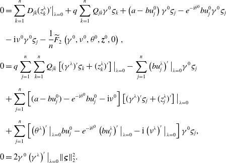 \begin{equation} \begin{split} \displaystyle 0&=\sum _{k=1}^n D_{jk}(z^\lambda _{k})'\big |_{\lambda =0}+q\sum _{k=1}^{n}Q_{jk}\gamma ^0 \varsigma _k +\left (a-bu^0_j\right )\gamma ^0 \varsigma _j - e^{{-\textrm{i}}\theta ^0}bu^0_j\gamma ^0 \varsigma _j\\[5pt] \displaystyle &-\textrm{i}\nu ^0\gamma ^0 \varsigma _j-\frac{1}{n}\widetilde{F}_2\left (\gamma ^0,\nu ^0,\theta ^0,{{\boldsymbol{z}}}^0,0\right ),\\[5pt] \displaystyle 0&=q \sum _{j=1}^n\sum _{k=1}^n Q_{jk}\left [(\gamma ^\lambda )'\varsigma _k+(z^\lambda _{k})'\right ]\big |_{\lambda =0}- \sum _{j=1}^n\left (bu^\lambda _j\right )'\big |_{\lambda =0}\gamma ^0 \varsigma _j \\[5pt] \displaystyle &+ \sum _{j=1}^n\left [(a-bu^0_j)-e^{{-\textrm{i}}\theta ^0}bu^0_j-\textrm{i}\nu ^0\right ]\left [(\gamma ^\lambda )'\varsigma _j +(z^\lambda _{j})'\right ]\big |_{\lambda =0}\\[5pt] \displaystyle &+ \sum _{j=1}^n\left [ \left (\theta ^\lambda \right )'\big |_{\lambda =0}bu^0_j- e^{{-\textrm{i}}\theta ^0}\left (bu^\lambda _j\right )'\big |_{\lambda =0}-\textrm{i}\left (\nu ^\lambda \right )'\big |_{\lambda =0}\right ]\gamma ^0 \varsigma _j, \\[5pt] \displaystyle 0&=2\gamma ^0\left (\gamma ^\lambda \right )'\big |_{\lambda =0}\|\boldsymbol{\varsigma }\|^2_2. \end{split} \end{equation}
By the third equation of (5.2), we have $\left (\gamma ^\lambda \right )'\big |_{\lambda =0}=0$
. Then plugging
$\left (\gamma ^\lambda \right )'\big |_{\lambda =0}=0$
. Then plugging $\left (\gamma ^\lambda \right )'\big |_{\lambda =0}=0$
into the first and second equations of (5.2), and noticing that
$\left (\gamma ^\lambda \right )'\big |_{\lambda =0}=0$
into the first and second equations of (5.2), and noticing that $\left (\gamma ^0,\nu ^0,\theta ^0\right )=\left (1,a-\displaystyle \frac{q}{n},\displaystyle \frac{\pi }{2}\right )$
,
$\left (\gamma ^0,\nu ^0,\theta ^0\right )=\left (1,a-\displaystyle \frac{q}{n},\displaystyle \frac{\pi }{2}\right )$
, ${{\boldsymbol{z}}}'\in (\widetilde{X}_1)_{\mathbb{C}}$
and
${{\boldsymbol{z}}}'\in (\widetilde{X}_1)_{\mathbb{C}}$
and $\widetilde{F}_2\left (\gamma ^0,\nu ^0,\theta ^0,{{\boldsymbol{z}}}^0,0\right )=0$
, we have
$\widetilde{F}_2\left (\gamma ^0,\nu ^0,\theta ^0,{{\boldsymbol{z}}}^0,0\right )=0$
, we have
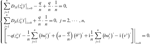 \begin{equation*} \begin{cases} \displaystyle \sum _{j=1}^n D_{1k}(z^\lambda _{k})'\big |_{\lambda =0}-\frac{q}{n}+\frac{q}{n}\cdot \frac{1}{n}=0,\\[5pt] \displaystyle \sum _{j=1}^n D_{jk}(z^\lambda _{k})'\big |_{\lambda =0}+\frac{q}{n}\cdot \frac{1}{n}=0,\;\;j=2,\cdots, n,\\[5pt] \displaystyle \left . \left [-q(z^\lambda _{n})'-\frac{1}{n}\sum _{j=1}^n\left (bu^\lambda _j\right )'+ \left (a-\frac{q}{n}\right )\left (\theta ^\lambda \right )'+ \displaystyle \textrm{i}\frac{1}{n}\sum _{j=1}^n \left (bu^\lambda _j\right )'-\textrm{i}\left (\nu ^\lambda \right )'\right ]\right |_{\lambda =0}=0. \end{cases} \end{equation*}
This combined with (2.20) and Proposition 5.4 in the appendix implies that
 \begin{equation*} \displaystyle \left (z^\lambda _n\right )'\big |_{\lambda =0}=\frac {q(n+1)(n-1)}{6n},\;\;\left (\nu ^\lambda \right )'\big |_{\lambda =0}=-\frac {q^2(n+1)(n-1)}{6n},\;\; \left (\theta ^\lambda \right )'\big |_{\lambda =0}=0. \end{equation*}
Then, by Theorem 3.13, we have
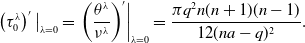 \begin{equation*} \displaystyle \left (\tau ^\lambda _0\right )'\big |_{\lambda =0}=\left .\left (\frac {\theta ^{\lambda }}{\nu ^{\lambda }}\right )'\right |_{\lambda =0} =\frac {\pi q^2n(n+1)(n-1)}{12(na-q)^2}. \end{equation*}
Now we consider (ii). By Lemmas 3.11, 3.12 and Theorem 3.13, we see that
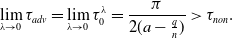 \begin{equation*}\displaystyle \lim _{\lambda \to 0}\tau _{adv}=\displaystyle \lim _{\lambda \to 0}\tau _0^\lambda =\displaystyle \frac {\pi }{2(a-\frac {q}{n})}\gt \tau _{non}.\end{equation*}
This, combined with (i), implies that (ii) holds. This completes the proof.
Then we consider the case of small diffusion rate.
Proposition 5.3.
Assume that $q\in (0,a)$
. Then, for
$q\in (0,a)$
. Then, for $d\in (0,\tilde d_2]$
with
$d\in (0,\tilde d_2]$
with $\tilde d_2\ll 1$
, the first Hopf bifurcation value of model
(1.5) is
$\tilde d_2\ll 1$
, the first Hopf bifurcation value of model
(1.5) is $\tau _{adv}=\tau ^d_{n,0}$
, where
$\tau _{adv}=\tau ^d_{n,0}$
, where $\tau ^d_{n,0}$
and
$\tau ^d_{n,0}$
and $\tilde d_2$
are defined in Theorem
3.9. Moreover, there exists
$\tilde d_2$
are defined in Theorem
3.9. Moreover, there exists $ \hat d_2\in (0,\tilde d_2]$
such that
$ \hat d_2\in (0,\tilde d_2]$
such that $\tau _{adv}\gt \tau _{non}$
for
$\tau _{adv}\gt \tau _{non}$
for $d\in (0,\hat d_2]$
.
$d\in (0,\hat d_2]$
.
Proof. By Theorems 3.9 and 4.3, we see that the first Hopf bifurcation value is $\tau _{adv}=\tau ^d_{n,0}$
, and
$\tau _{adv}=\tau ^d_{n,0}$
, and
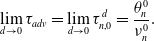 \begin{equation} \displaystyle \lim _{d\to 0}\tau _{adv}=\displaystyle \lim _{d\to 0}\tau ^d_{n,0}=\displaystyle \frac{\theta ^{0}_{n}}{\nu ^{0}_{n}}. \end{equation}
By Lemma 3.7 (ii), we see that $\displaystyle \frac{\theta ^{0}_{n}}{\nu ^{0}_{n}}\gt \frac{\pi }{2a}$
. This, combined with (5.3), implies that there exists
$\displaystyle \frac{\theta ^{0}_{n}}{\nu ^{0}_{n}}\gt \frac{\pi }{2a}$
. This, combined with (5.3), implies that there exists $ \hat d_2\in (0,\tilde d_2]$
such that
$ \hat d_2\in (0,\tilde d_2]$
such that $\tau _{adv}\gt \tau _{non}$
for
$\tau _{adv}\gt \tau _{non}$
for $d\in (0,\hat d_2]$
.
$d\in (0,\hat d_2]$
.
It follows from Propositions 5.2 and 5.3 that the first Hopf bifurcation value in advective environments is larger than that in non-advective environments if $d\gg 1$
or
$d\gg 1$
or $d\ll 1$
, see Figure 2. This result suggests that directed movements of the individuals inhibit the occurrence of Hopf bifurcation.
$d\ll 1$
, see Figure 2. This result suggests that directed movements of the individuals inhibit the occurrence of Hopf bifurcation.
Now we give some numerical simulations. We choose three patches, that is, $n=3$
, and set
$n=3$
, and set $a=1$
and
$a=1$
and $b=1$
. Then we can numerically compute the first Hopf bifurcation
$b=1$
. Then we can numerically compute the first Hopf bifurcation $\tau _{adv}$
for a wider range of parameters. For the case
$\tau _{adv}$
for a wider range of parameters. For the case $q\in (0,a)$
, we prove that large delay can also induce Hopf bifurcations for model (1.5) if
$q\in (0,a)$
, we prove that large delay can also induce Hopf bifurcations for model (1.5) if $0\lt d\ll 1$
or
$0\lt d\ll 1$
or $d\gg 1$
(Theorem 4.3 (ii) and (iii)). Then we compute that there exist three families of Hopf bifurcation curves
$d\gg 1$
(Theorem 4.3 (ii) and (iii)). Then we compute that there exist three families of Hopf bifurcation curves $\left \{\tau _{j,l}^d\right \}_{l=1}^\infty (j=1,2,3)$
. For simplicity, we only plot the first one for each family
$\left \{\tau _{j,l}^d\right \}_{l=1}^\infty (j=1,2,3)$
. For simplicity, we only plot the first one for each family $\left \{\tau _{j,l}^d\right \}_{l=1}^\infty (j=1,2,3)$
in Figure 4.
$\left \{\tau _{j,l}^d\right \}_{l=1}^\infty (j=1,2,3)$
in Figure 4.
Then $\tau _{adv}=\displaystyle \min _{1\le j\le 3}{\tau _{j,0}^d}$
, and it exists for
$\tau _{adv}=\displaystyle \min _{1\le j\le 3}{\tau _{j,0}^d}$
, and it exists for $d\in (0,\infty )$
, which implies that delay-induced Hopf bifurcation may occur for
$d\in (0,\infty )$
, which implies that delay-induced Hopf bifurcation may occur for $d\in (0,\infty )$
. Actually, we choose
$d\in (0,\infty )$
. Actually, we choose $d=0.06,1.5,20,150$
and numerically show that there exist periodic solutions; see Figure 5.
$d=0.06,1.5,20,150$
and numerically show that there exist periodic solutions; see Figure 5.
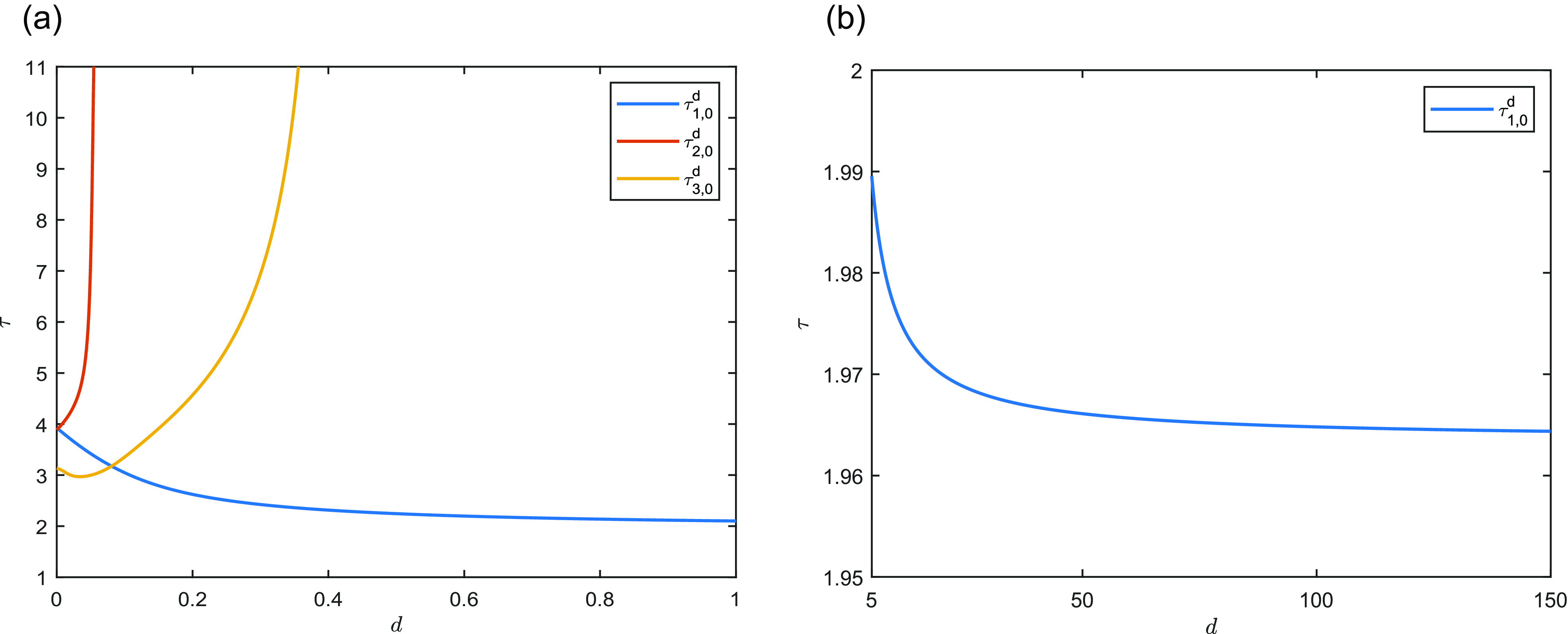
Figure 4. The relation between Hopf bifurcation values and dispersal rate $d$
for the case
$d$
for the case $q\in (0,a)$
with
$q\in (0,a)$
with $a=1$
,
$a=1$
, $b=1$
and
$b=1$
and $q=0.6$
. (a)
$q=0.6$
. (a) $d\in (0,1]$
; (b)
$d\in (0,1]$
; (b) $d\in [5,150]$
.
$d\in [5,150]$
.
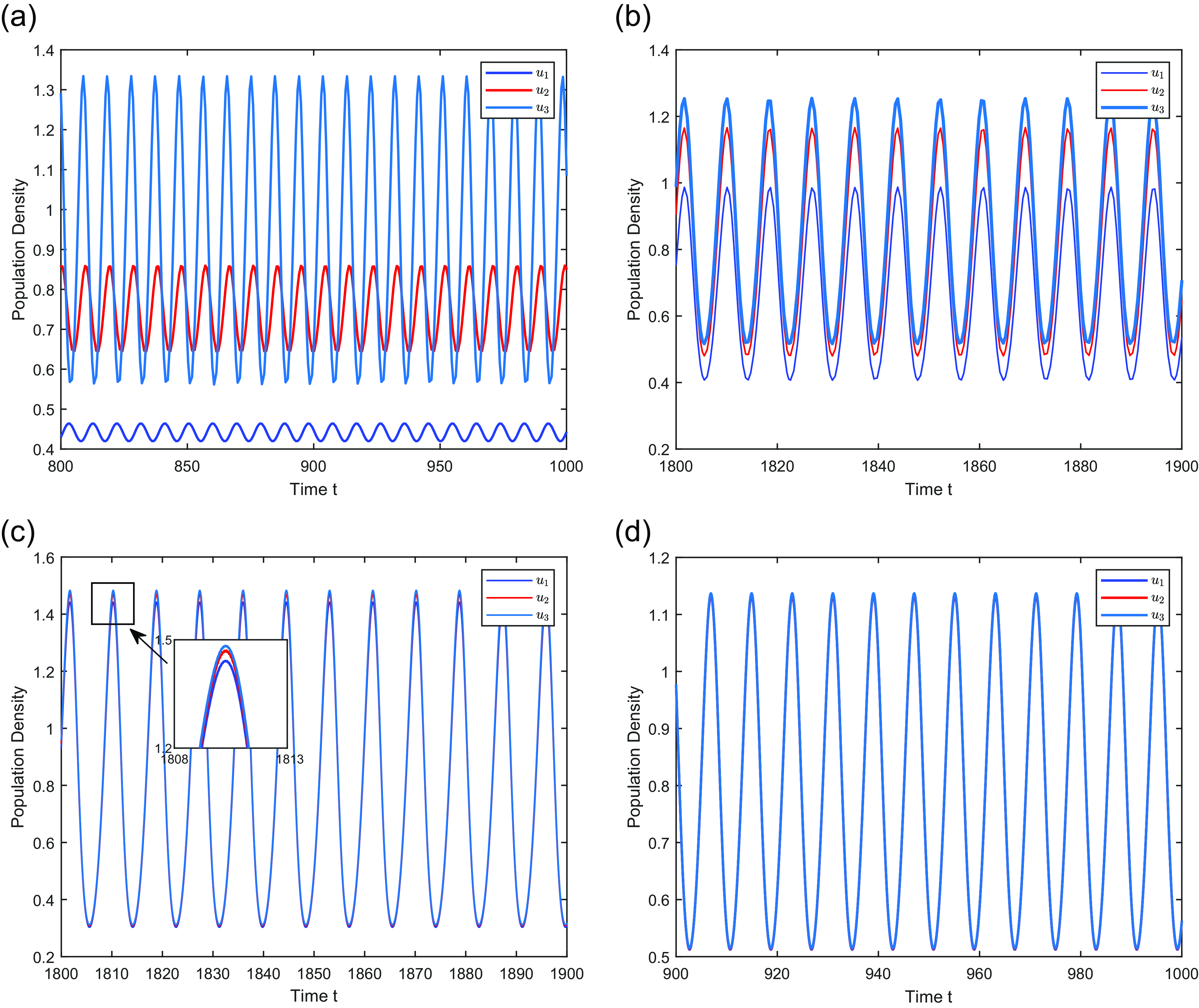
Figure 5. Periodic solutions induced by a Hopf bifurcation with $a=1$
,
$a=1$
, $b=1$
and
$b=1$
and $q=0.6$
. (a)
$q=0.6$
. (a) $d=0.06$
and
$d=0.06$
and $\tau =3.1$
; (b)
$\tau =3.1$
; (b) $d=1.5$
and
$d=1.5$
and $\tau =2.1$
; (c)
$\tau =2.1$
; (c) $d=20$
and
$d=20$
and $\tau =2.1$
; (d)
$\tau =2.1$
; (d) $d=150$
and
$d=150$
and $\tau =2.0$
.
$\tau =2.0$
.
For the case $q\in (a,na)$
, we prove that large delay can induce Hopf bifurcations for model (1.5) if
$q\in (a,na)$
, we prove that large delay can induce Hopf bifurcations for model (1.5) if $0\lt d-d_q^*\ll 1$
or
$0\lt d-d_q^*\ll 1$
or $d\gg 1$
(Theorem 4.3 (i) and (iii)). In Figure 6, we plot
$d\gg 1$
(Theorem 4.3 (i) and (iii)). In Figure 6, we plot $\tau _{adv}$
for this case, and it exists for
$\tau _{adv}$
for this case, and it exists for $d\in (d_q^*,\infty )$
, which implies that delay-induced Hopf bifurcation may occur for
$d\in (d_q^*,\infty )$
, which implies that delay-induced Hopf bifurcation may occur for $d\in (d_q^*,\infty )$
.
$d\in (d_q^*,\infty )$
.
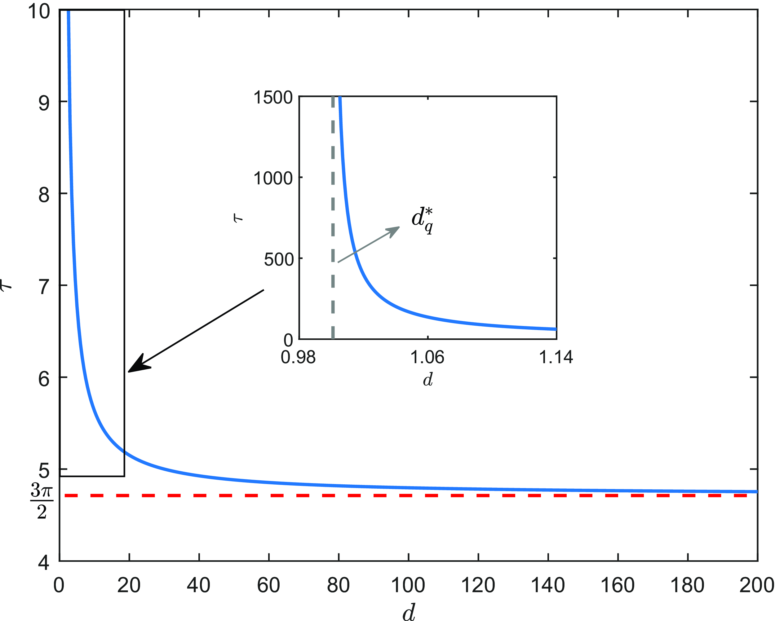
Figure 6. The relation between Hopf bifurcation value and dispersal rate $d$
for the case
$d$
for the case $q\in (a,na)$
with
$q\in (a,na)$
with $a=1$
,
$a=1$
, $b=1$
and
$b=1$
and $q=2$
.
$q=2$
.
By Figures 4 and 6, we conjecture that $\tau _{adv}$
change monotonicity once with respect to
$\tau _{adv}$
change monotonicity once with respect to $d$
. In fact, by Proposition 5.2,
$d$
. In fact, by Proposition 5.2, $\tau _{adv}$
is decreasing in
$\tau _{adv}$
is decreasing in $d$
when
$d$
when $d$
is sufficiently large. Moreover, in Propositions 5.2 and 5.3, we show that
$d$
is sufficiently large. Moreover, in Propositions 5.2 and 5.3, we show that $\tau _{adv}\gt \tau _{non}$
, which suggests that directed movements of the individuals inhibit the occurrence of Hopf bifurcation. To illustrate this phenomenon, we fix
$\tau _{adv}\gt \tau _{non}$
, which suggests that directed movements of the individuals inhibit the occurrence of Hopf bifurcation. To illustrate this phenomenon, we fix $\tau =1.6$
,
$\tau =1.6$
, $d=1.14$
and choose the same initial values for
$d=1.14$
and choose the same initial values for $q=0$
and
$q=0$
and $q=2$
. As is shown in Figure 7, periodic oscillations disappear for
$q=2$
. As is shown in Figure 7, periodic oscillations disappear for $q\ne 0$
.
$q\ne 0$
.
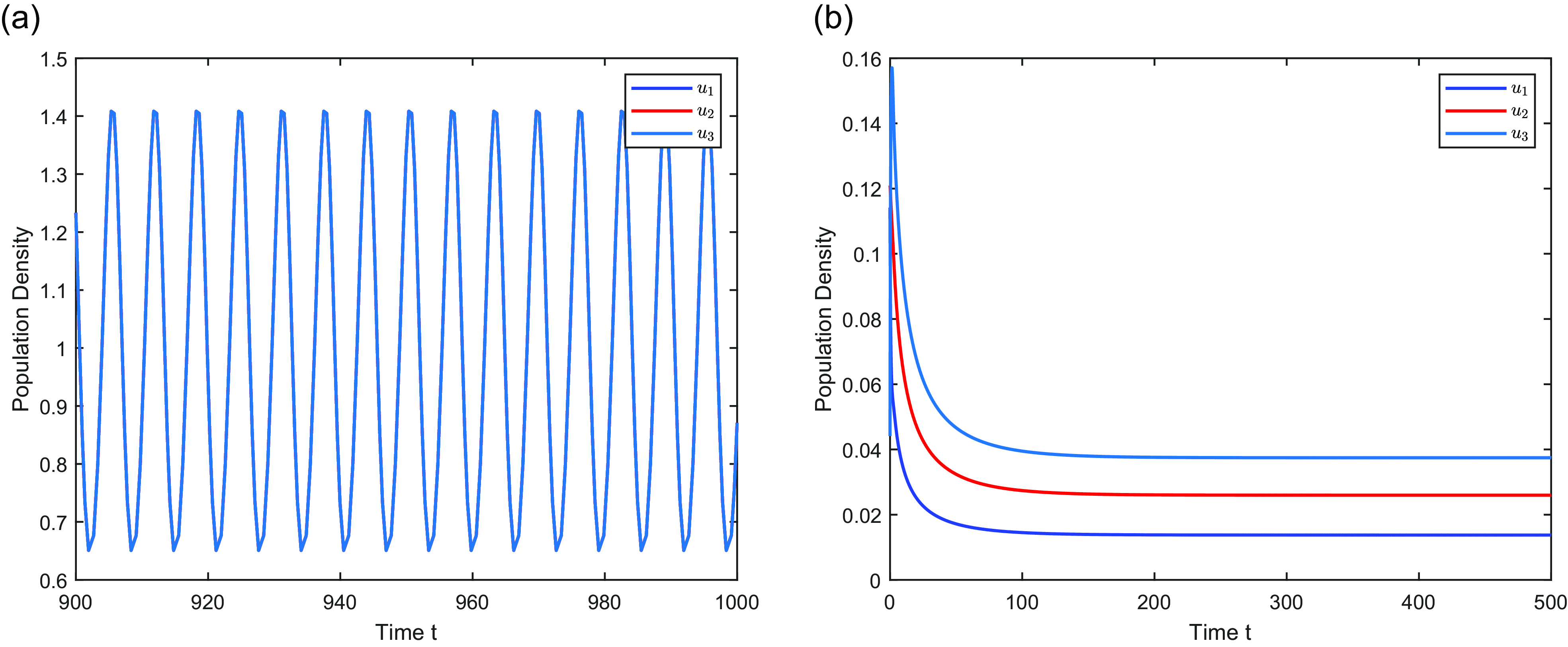
Figure 7.
Directed drift rate $q$
inhibit the occurrence of Hopf bifurcation. Here,
$q$
inhibit the occurrence of Hopf bifurcation. Here, $a=1$
,
$a=1$
, $b=1$
,
$b=1$
, $d=1.14$
and
$d=1.14$
and $\tau =1.6$
. (a)
$\tau =1.6$
. (a) $ q=0$
; (b)
$ q=0$
; (b) $q=2$
.
$q=2$
.
We remark that model (1.5) is a discrete form of model (1.6), where $D_{jk}$
is defined in (1.3) and
$D_{jk}$
is defined in (1.3) and
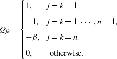 \begin{equation} Q_{jk}= \begin{cases} 1, & j=k+1, \\[5pt] -1, & j=k=1,\cdots, n-1, \\[5pt] -\beta, &j=k=n,\\[5pt] 0, & \text{ otherwise. } \end{cases} \end{equation}
In this paper, we consider the case $\beta =1$
, and it is natural to ask whether
$\beta =1$
, and it is natural to ask whether $\beta$
(the population loss rate at the downstream end) affects Hopf bifurcations. Then we consider this problem from the point view of numerical simulations and choose
$\beta$
(the population loss rate at the downstream end) affects Hopf bifurcations. Then we consider this problem from the point view of numerical simulations and choose
 \begin{equation*}n=3 \;\;\text {(three patches)},\;\;a=1,\;\; b=1,\;\;q=0.6,\;\;d=2.\end{equation*}
If $\beta =1$
, we compute that
$\beta =1$
, we compute that $\tau _{adv}\approx 2.03$
. Then set
$\tau _{adv}\approx 2.03$
. Then set $\tau =2.1$
, we show that there also exists periodic solutions for
$\tau =2.1$
, we show that there also exists periodic solutions for $\beta =0.9$
, and periodic oscillations disappear for
$\beta =0.9$
, and periodic oscillations disappear for $\beta =1.5$
, see Figure 8. Then, we conjecture that if the positive equilibrium of (1.5) exists, the minimum Hopf bifurcation value for the case
$\beta =1.5$
, see Figure 8. Then, we conjecture that if the positive equilibrium of (1.5) exists, the minimum Hopf bifurcation value for the case $\beta \gt 1$
(resp.
$\beta \gt 1$
(resp. $\beta \lt 1$
) is larger (resp. smaller) than that for the case
$\beta \lt 1$
) is larger (resp. smaller) than that for the case $\beta =1$
.
$\beta =1$
.


Ethical standards
Not applicable.
Competing interests
The authors declare that they have no conflict of interest.
Author contributions
All authors contributed to the study conception and design. SC developed the idea for the study. The manuscript was written by LW, SZ and SC, and LW and SZ prepared Figures 1 –7. All authors read and approved the final manuscript.
Financial support
This research is Taishan Scholars Program of Shandong Province (No. tsqn 202306137), National Natural Science Foundation of China (Nos. 12171117 and 12101161) and Heilongjiang Provincial Natural Science Foundation of China (No. YQ2021A007).
Data availability statement
All data generated or analysed during this study are included in this published article.
Appendix
In the appendix, we show the following result by linear algebraic techniques.
Proposition 5.4.
Let $D=(D_{jk})$
with
$D=(D_{jk})$
with $D_{jk}$
defined in
(1.3), and let
$D_{jk}$
defined in
(1.3), and let $\widetilde{X}_1$
be defined in
(2.18). Assume that
$\widetilde{X}_1$
be defined in
(2.18). Assume that $D{{\boldsymbol{y}}}={\boldsymbol{a}}$
with
$D{{\boldsymbol{y}}}={\boldsymbol{a}}$
with ${{\boldsymbol{a}}},{{\boldsymbol{y}}}\in \widetilde{X}_1$
. Then
${{\boldsymbol{a}}},{{\boldsymbol{y}}}\in \widetilde{X}_1$
. Then
 \begin{equation} y_n=\frac{1}{n}\sum _{k=1}^{n-1}k\left (\sum _{j=1}^k a_j\right ). \end{equation}
Especially, if $a_2=\cdots =a_n$
, then
$a_2=\cdots =a_n$
, then
 \begin{equation} y_n=\frac{n(n-1)}{2}a_1+\frac{(n-2)(n-1)n}{3}a_2 \end{equation}
Proof. Since $D{{\boldsymbol{y}}}={\boldsymbol{a}}$
and
$D{{\boldsymbol{y}}}={\boldsymbol{a}}$
and ${{\boldsymbol{y}}}\in \widetilde{X}_1$
, we have
${{\boldsymbol{y}}}\in \widetilde{X}_1$
, we have
 \begin{equation} -y_1+y_2=a_1, \end{equation}
 \begin{equation}y_{j-1}-2y_{j}+y_{j+1}=a_j,\;\;j=2,\cdots, n-1, \end{equation}
and
 \begin{equation} \sum _{j=1}^ny_j=0. \end{equation}
Summing the first $k$
equations in (5.7), we find
$k$
equations in (5.7), we find
 \begin{equation} -y_k+y_{k+1}=\sum _{j=1}^{k}a_j, \;\;k=1,\cdots, n-1. \end{equation}
Multiplying (5.9) by $k$
and summing these over all
$k$
and summing these over all $k$
yields
$k$
yields
 \begin{equation*} -\sum _{j=1}^{n-1}y_j+(n-1)y_n=\sum _{k=1}^{n-1}k\left (\sum _{j=1}^k a_j\right ). \end{equation*}
This combined with (5.8) implies that (5.5) holds.
Now we consider (5.6). A direct computation yields
 \begin{equation*} \begin{split} y_n=&\left (\sum _{j=1}^{n-1}j\right )a_1+\left (\sum _{j=1}^{n-2} j(j+1)\right )a_2\\[5pt] =&\frac{n(n-1)}{2}a_1+\frac{(n-2)(n-1)n}{3}a_2, \end{split} \end{equation*}
where we have used $\sum _{j=1}^{n} j(j+1)=\frac{n(n+1)(n+2)}{3}$
in the last step. This completes the proof.
$\sum _{j=1}^{n} j(j+1)=\frac{n(n+1)(n+2)}{3}$
in the last step. This completes the proof.


 Open access