1. Introduction
Let
![]() $X=\{X_t,t \in \mathbb{R}_+\}$
be an irreducible continuous-time Markov chain (CTMC) on state space
$X=\{X_t,t \in \mathbb{R}_+\}$
be an irreducible continuous-time Markov chain (CTMC) on state space
![]() $E=\mathbb{Z}_+$
with transition function
$E=\mathbb{Z}_+$
with transition function
![]() $P^t(i,j)$
and regular q-matrix
$P^t(i,j)$
and regular q-matrix
![]() $Q=(q(i,j))$
. Let X be positive recurrent with the unique invariant distribution
$Q=(q(i,j))$
. Let X be positive recurrent with the unique invariant distribution
![]() $\pi$
. Suppose that X is perturbed to another irreducible and regular CTMC
$\pi$
. Suppose that X is perturbed to another irreducible and regular CTMC
![]() $\tilde{X}=\{\tilde{X}_t,t \in \mathbb{R}_+\}$
with transition function
$\tilde{X}=\{\tilde{X}_t,t \in \mathbb{R}_+\}$
with transition function
![]() $\tilde{P}^t(i,j)$
and q-matrix
$\tilde{P}^t(i,j)$
and q-matrix
![]() $\tilde{Q}=(\tilde{q}(i,j))$
. Denote by
$\tilde{Q}=(\tilde{q}(i,j))$
. Denote by
![]() $p^t$
and
$p^t$
and
![]() $\tilde{p}^t$
the state probability vectors of
$\tilde{p}^t$
the state probability vectors of
![]() $X_t$
and
$X_t$
and
![]() $\tilde{X}_t$
, respectively. In particular, when
$\tilde{X}_t$
, respectively. In particular, when
![]() $t=0$
, they represent the initial distributions. Let
$t=0$
, they represent the initial distributions. Let
![]() $\Delta=\tilde{Q}-Q$
be the perturbation of the q-matrix. As is shown in [Reference Liu14], a small perturbation may result in a big change in the stability. Hence, it is meaningful to find sufficient conditions that guarantee the stability and, moreover, obtain quantitative bounds on the difference between two chains when the stability is robust.
$\Delta=\tilde{Q}-Q$
be the perturbation of the q-matrix. As is shown in [Reference Liu14], a small perturbation may result in a big change in the stability. Hence, it is meaningful to find sufficient conditions that guarantee the stability and, moreover, obtain quantitative bounds on the difference between two chains when the stability is robust.
For discrete-time Markov chains (DTMCs), perturbation bounds with respect to the V-norms (as defined in Section 2) were developed in the seminal work of [Reference Kartashov10, Reference Kartashov11]. Recent advances in this direction can be found in [Reference Abbas, Berkhout and Heidergott1, Reference Liu13, Reference Mouhoubi23, Reference Mouhoubi and Aissani24]. For CTMCs, the V-normwise perturbation bounds have also received recent attention, see [Reference Heidergott, Hordijk and Leder5, Reference Jiang, Liu and Tang9, Reference Liu14, Reference Liu and Li15, Reference Masuyama19]. However, as we will see, we have to be careful to deal with a CTMC with an unbounded generator for which the V-normwise results might be invalid. For instance, consider the following linear birth and death process with catastrophes (see [Reference Pollett, Zhang and Cairns25]) on state space
![]() $E=\mathbb{Z}_+$
, whose q-matrix is given by
$E=\mathbb{Z}_+$
, whose q-matrix is given by
 \begin{equation}Q=\left(\begin{array}{c@{\quad}c@{\quad}c@{\quad}c@{\quad}c}-b & b & 0 & 0 & \cdots\\[5pt] a & -(a+b) & b & 0 & \cdots\\[5pt] d_2 & 2a & -2(a+b)-d_2 & 2b & \cdots\\[5pt] d_3 & 0 & 3a & -3(a+b)-d_3 & \cdots\\[5pt] \vdots & \vdots & \vdots & \vdots & \ddots\end{array}\right).\end{equation}
The model parameters are usually estimated based on statistical data, which naturally causes a small deviation from the true value. Hence, it is reasonable to assume that there exist perturbations imposed on the parameters. Specifically, we assume that the parameters
![]() $d_i$
, a, and b in (1) are perturbed to be
$d_i$
, a, and b in (1) are perturbed to be
![]() $d_i+\varepsilon$
,
$d_i+\varepsilon$
,
![]() $a+\varepsilon$
, and
$a+\varepsilon$
, and
![]() $b+\varepsilon$
, respectively. As a consequence, the perturbation matrix
$b+\varepsilon$
, respectively. As a consequence, the perturbation matrix
![]() $\Delta(\varepsilon)$
, given by
$\Delta(\varepsilon)$
, given by
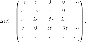 \begin{equation}\Delta(\varepsilon)=\left(\begin{array}{c@{\quad}c@{\quad}c@{\quad}c@{\quad}c}-\varepsilon & \varepsilon & 0 & 0 & \cdots\\[5pt] \varepsilon & -2\varepsilon & \varepsilon & 0 & \cdots\\[5pt] \varepsilon & 2\varepsilon & -5\varepsilon & 2\varepsilon & \cdots\\[5pt] \varepsilon & 0 & 3\varepsilon & -7\varepsilon & \cdots\\[5pt] \vdots & \vdots & \vdots & \vdots & \ddots\end{array}\right),\end{equation}
is unbounded. Observe that, for any finite function
![]() $V\colon E\rightarrow [1,\infty)$
,
$V\colon E\rightarrow [1,\infty)$
,
This shows that the V-normwise perturbation bound (see [Reference Liu14])
where
![]() $C(Q,\tilde{Q})$
is known as a positive condition number, becomes uninformative since its upper bound is always
$C(Q,\tilde{Q})$
is known as a positive condition number, becomes uninformative since its upper bound is always
![]() $\infty$
. From this example, we see that the V-norm may be too restrictive to characterize unbounded perturbation problems.
$\infty$
. From this example, we see that the V-norm may be too restrictive to characterize unbounded perturbation problems.
For perturbation analysis of DTMCs in a weak sense, [Reference Shardlow and Stuart27] first developed a perturbation theory for geometrically ergodic Markov chains which requires controlling perturbations of iterated transition kernels in a weak 1,V-norm (see Section 2 for the detailed definition). Subsequently, [Reference Herve and Ledoux6] obtained explicit bounds on the stationary distributions between two Markov chains via weak perturbation theory. [Reference Rudolf and Schweizer26] derived the bounds on finite-step state distributions by using an approach based on drift conditions and ergodic convergence rate. [Reference Medina-Aguayo, Rudolf and Schweizer20] further refined and extended this result and applied it to the Monte Carlo within Metropolis algorithms. We aim to develop perturbation bounds on
![]() $\|\tilde{p}^t-p^t\|_1$
in terms of the perturbation
$\|\tilde{p}^t-p^t\|_1$
in terms of the perturbation
![]() $\Delta$
in the weak 1, V-norm for CTMCs.
$\Delta$
in the weak 1, V-norm for CTMCs.
It is worth noting that the generators of CTMCs can be unbounded, like (1) mentioned above, for which it is usually infeasible to extend the results of DTMCs to the continuous-time case by the technique of uniformized chains or h-skeleton chains. Using a uniformized chain introduces the quantity
![]() $\sup_{i}|q(i,i)|$
which is infinite for unbounded CTMCs, while using h-skeleton chains will involve a relation between
$\sup_{i}|q(i,i)|$
which is infinite for unbounded CTMCs, while using h-skeleton chains will involve a relation between
![]() $\tilde{P}^h-{P}^h$
and
$\tilde{P}^h-{P}^h$
and
![]() $\tilde{Q}-Q$
which cannot be determined explicitly. In this paper, we develop an approach that combines the ergodicity coefficients, drift functions, and the technique of augmented truncations to investigate the perturbation in the weak sense.
$\tilde{Q}-Q$
which cannot be determined explicitly. In this paper, we develop an approach that combines the ergodicity coefficients, drift functions, and the technique of augmented truncations to investigate the perturbation in the weak sense.
This paper is organized as follows. Section 2 contains some preliminaries, such as the definitions of V-norms and 1,V-norms, and the properties of ergodicity coefficients. In Section 3, we obtain the perturbation bounds for strongly ergodic CTMCs, in particular for those satisfying Doeblin or stochastically monotone conditions. In Section 4, we present the estimates for exponentially ergodic CTMCs, and further apply our results to stochastically monotone CTMCs. Finally, some conclusions are listed in Section 5.
2. Preliminaries
For a finite measure
![]() $\mu$
and
$\mu$
and
![]() $V\colon E \rightarrow [1,\infty)$
, let
$V\colon E \rightarrow [1,\infty)$
, let
![]() $\mu(V)=\sum_{i\in E}\mu(i)V(i)$
and define its V-norm to be
$\mu(V)=\sum_{i\in E}\mu(i)V(i)$
and define its V-norm to be
![]() $\|\mu\|_V=\sum_{i\in E}|\mu(i)|V(i)$
. The V-norm for any matrix
$\|\mu\|_V=\sum_{i\in E}|\mu(i)|V(i)$
. The V-norm for any matrix
![]() $R=(R(i,j))$
on
$R=(R(i,j))$
on
![]() $E\times E$
is given by
$E\times E$
is given by
When
![]() $V\equiv 1$
, we replace the subscript V in
$V\equiv 1$
, we replace the subscript V in
![]() $\|\mu\|_V$
and
$\|\mu\|_V$
and
![]() $\|R\|_V$
by 1. Note that
$\|R\|_V$
by 1. Note that
![]() $\|\mu R\|_V\leq \|\mu\|_V \|R\|_V$
and
$\|\mu R\|_V\leq \|\mu\|_V \|R\|_V$
and
![]() $\|AB\|_V\leq \|A\|_V \|B\|_V$
for any pair of matrices A and B on
$\|AB\|_V\leq \|A\|_V \|B\|_V$
for any pair of matrices A and B on
![]() $E\times E$
. In addition, we define the weak 1,V-norm (see [Reference Ferre, Herve and Ledoux3]) for any matrix R by
$E\times E$
. In addition, we define the weak 1,V-norm (see [Reference Ferre, Herve and Ledoux3]) for any matrix R by
The V-norm ergodicity coefficient of the transition matrix
![]() $P^t$
is defined by
$P^t$
is defined by
see [Reference Ipsen and Selee7, Reference Kartashov12, Reference Mao, Zhang and Zhang18]. When
![]() $V\equiv 1$
,
$V\equiv 1$
,
![]() $\tau_1(P^t)$
is the classical Dobrushin coefficient. [Reference Mao, Zhang and Zhang18, Proposition 2.1] gives some properties of V-norm ergodicity coefficients. Based on their results, we can easily obtain the following lemma on the contractivity of V-norm ergodicity coefficients.
$\tau_1(P^t)$
is the classical Dobrushin coefficient. [Reference Mao, Zhang and Zhang18, Proposition 2.1] gives some properties of V-norm ergodicity coefficients. Based on their results, we can easily obtain the following lemma on the contractivity of V-norm ergodicity coefficients.
Lemma 1. Let
![]() $\mu$
,
$\mu$
,
![]() $\nu$
be two measures on E satisfying
$\nu$
be two measures on E satisfying
![]() $(\mu-\nu)\mathbf{1}=0$
and
$(\mu-\nu)\mathbf{1}=0$
and
![]() $\|\mu-\nu\|_V<\infty$
, where
$\|\mu-\nu\|_V<\infty$
, where
![]() $\mathbf{1}$
is a column vector of 1s. For the transition matrix
$\mathbf{1}$
is a column vector of 1s. For the transition matrix
![]() $P^t$
,
$P^t$
,
Proof. Let
![]() $R=\mathbf{1}(\mu-\nu)$
. Since
$R=\mathbf{1}(\mu-\nu)$
. Since
![]() $(\mu-\nu)\mathbf{1}=0$
and
$(\mu-\nu)\mathbf{1}=0$
and
![]() $\|\mu-\nu\|_V<\infty$
, we have
$\|\mu-\nu\|_V<\infty$
, we have
and
It follows from [Reference Mao, Zhang and Zhang18, Proposition 2.1(iii)] that
The assertion follows immediately by the fact that
![]() $\inf_{i\in E}V(i)>0$
.
$\inf_{i\in E}V(i)>0$
.
In the following, we present the definitions of strong and exponential ergodicity.
Definition 1.
![]() $P^t$
is called strongly ergodic if there exist positive constants
$P^t$
is called strongly ergodic if there exist positive constants
![]() $\rho <1$
and
$\rho <1$
and
![]() $C<\infty$
such that, for any i and t,
$C<\infty$
such that, for any i and t,
Definition 2.
![]() $P^t$
is called exponentially ergodic if there exists a positive constant
$P^t$
is called exponentially ergodic if there exists a positive constant
![]() $\rho <1$
and a finite function
$\rho <1$
and a finite function
![]() $C\colon E\rightarrow (0, \infty)$
such that, for any i and t,
$C\colon E\rightarrow (0, \infty)$
such that, for any i and t,
Definition 3.
![]() $P^t$
is called V-uniformly ergodic if there exist positive constants
$P^t$
is called V-uniformly ergodic if there exist positive constants
![]() $\rho <1$
,
$\rho <1$
,
![]() $C < \infty$
and a finite function
$C < \infty$
and a finite function
![]() $V\colon E\rightarrow [1, \infty)$
such that, for any i and t,
$V\colon E\rightarrow [1, \infty)$
such that, for any i and t,
For irreducible CTMCs, it is well known that exponential ergodicity is equivalent to V-uniform ergodicity [Reference Hart and Tweedie4, Theorem 3.2]. Observe that the V-uniform ergodicity of
![]() $P^t$
implies a suitable upper bound on its V-norm ergodicity coefficient
$P^t$
implies a suitable upper bound on its V-norm ergodicity coefficient
![]() $\tau_V(P^t)$
. Applying arguments similar to [Reference Rudolf and Schweizer26, Lemma 3.2], we have the following statement.
$\tau_V(P^t)$
. Applying arguments similar to [Reference Rudolf and Schweizer26, Lemma 3.2], we have the following statement.
Lemma 2. If
![]() $P^t$
is V-uniformly ergodic, then
$P^t$
is V-uniformly ergodic, then
![]() $\tau_V(P^t)\leq C \rho^t$
.
$\tau_V(P^t)\leq C \rho^t$
.
When
![]() $V \equiv 1$
,
$V \equiv 1$
,
![]() $\tau_V(P^t)=\tau_1(P^t)$
and hence Lemma 2 generalizes the classical Dobrushin coefficient. That is, if
$\tau_V(P^t)=\tau_1(P^t)$
and hence Lemma 2 generalizes the classical Dobrushin coefficient. That is, if
![]() $P^t$
is strongly ergodic, then
$P^t$
is strongly ergodic, then
![]() $\tau_1(P^t)\leq C \rho^t$
.
$\tau_1(P^t)\leq C \rho^t$
.
3. Perturbation analysis for strongly ergodic CTMCs
In this section, we obtain perturbation bounds for strongly ergodic CTMCs by the technique of augmented truncations. First, we obtain the results for finite state spaces with an approach based on ergodicity coefficients and drift functions. Then we derive those of infinitely countable state spaces by letting the truncation size tend to infinity. In particular, the results are applied to get the explicit perturbation bounds for CTMCs satisfying Doeblin or stochastically monotone conditions. Some examples are presented to illustrate our results.
Our results in this section mainly rely on the following two assumptions.
Assumption 1.
![]() $P^t$
is strongly ergodic with positive constants
$P^t$
is strongly ergodic with positive constants
![]() $\rho <1$
and
$\rho <1$
and
![]() $C<\infty$
.
$C<\infty$
.
Assumption 2. There exists a finite function
![]() $V\colon E \rightarrow [1, \infty)$
and positive constants
$V\colon E \rightarrow [1, \infty)$
and positive constants
![]() $\delta$
and
$\delta$
and
![]() $L <\infty$
such that
$L <\infty$
such that
![]() $(\tilde{Q}V)(i)\leq -\delta V(i)+L$
.
$(\tilde{Q}V)(i)\leq -\delta V(i)+L$
.
3.1. Finite state spaces
Let
![]() $E_n=\{0,1,2,\ldots,n\}$
,
$E_n=\{0,1,2,\ldots,n\}$
,
![]() $n\geq 0$
. We are now in a position to present the perturbation bounds for CTMCs on finite state space
$n\geq 0$
. We are now in a position to present the perturbation bounds for CTMCs on finite state space
![]() $E_n$
.
$E_n$
.
Proposition 1. Let X be an irreducible CTMC on finite state space
![]() $E_n$
. Suppose that Assumptions 1 and 2 hold. Then we have
$E_n$
. Suppose that Assumptions 1 and 2 hold. Then we have
where
![]() $\kappa = \max\{\tilde{p}^0(V),{L}/{\delta}\}$
.
$\kappa = \max\{\tilde{p}^0(V),{L}/{\delta}\}$
.
Proof. The vectors
![]() $\tilde{p}^t$
and
$\tilde{p}^t$
and
![]() $p^t$
satisfy the forward Kolmogorov equations
$p^t$
satisfy the forward Kolmogorov equations
Therefore, the vector
![]() $z_t=\tilde{p}^t-p^t$
is the solution to the initial-value problem
$z_t=\tilde{p}^t-p^t$
is the solution to the initial-value problem
which implies that
![]() $\tilde{p}^t - p^t = (\tilde{p}^0-p^0)P^t + \int_0^t\tilde{p}^{t-u}(\tilde{Q}-Q)P^u\,{\mathrm{d}} u$
, and
$\tilde{p}^t - p^t = (\tilde{p}^0-p^0)P^t + \int_0^t\tilde{p}^{t-u}(\tilde{Q}-Q)P^u\,{\mathrm{d}} u$
, and
see also the proof of [Reference Mitrophanov22, Theorem 2.1]. Since the state space
![]() $E_n$
is finite and
$E_n$
is finite and
![]() $(\tilde{p}^0-p^0)\mathbf{1}=0$
,
$(\tilde{p}^0-p^0)\mathbf{1}=0$
,
![]() $\tilde{p}^{t-u}(\tilde{Q}-Q)\mathbf{1}=0$
, it follows from Lemmas 1 and 2 that
$\tilde{p}^{t-u}(\tilde{Q}-Q)\mathbf{1}=0$
, it follows from Lemmas 1 and 2 that
 \begin{align*} \|(\tilde{p}^0-p^0)P^t\|_1 & \leq \|\tilde{p}^0-p^0\|_1 \cdot \tau_1(P^t) \leq C\rho^t\|\tilde{p}^0-p^0\|_1, \\[5pt] \|\tilde{p}^{t-u}(\tilde{Q}-Q)P^u\|_1 & \leq \|\tilde{p}^{t-u}(\tilde{Q}-Q)\|_1 \tau_1(P^u) . \end{align*}
We also have
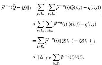 \begin{align*} \|\tilde{p}^{t-u}(\tilde{Q}-Q)\|_1 & = \sum_{j\in E_n}\Bigg|\sum_{i\in E_n}\tilde{p}^{t-u}(i)(\tilde{q}(i,j)-q(i,j))\Bigg| \\[5pt] & \leq \sum_{i\in E_n}\sum_{j\in E_n}\tilde{p}^{t-u}(i)|\tilde{q}(i,j)-q(i,j)| \\[5pt] & = \sum_{i\in E_n}\tilde{p}^{t-u}(i)\|\tilde{Q}(i,\cdot)-Q(i,\cdot)\|_1 \\[5pt] & \leq \|\Delta\|_{1,V}\sum_{i\in E_n} \tilde{p}^{t-u}(i)V(i). \end{align*}
Moreover, since
![]() $\tilde{Q}$
satisfies the drift condition
$\tilde{Q}$
satisfies the drift condition
![]() $\tilde{Q}V \leq -\delta V + L\mathbf{1}$
, we have
$\tilde{Q}V \leq -\delta V + L\mathbf{1}$
, we have
Using an induction argument yields
From this inequality, for
![]() $t-u\geq 0$
we can obtain
$t-u\geq 0$
we can obtain
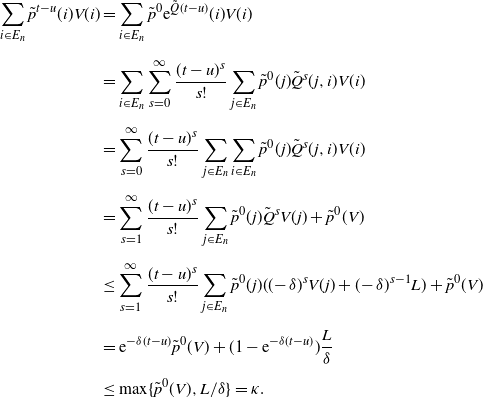 \begin{align} \sum_{i\in E_n}\tilde{p}^{t-u}(i)V(i) & = \sum_{i\in E_n}\tilde{p}^0{\mathrm{e}}^{\tilde{Q}(t-u)}(i)V(i) \nonumber \\[5pt] & = \sum_{i\in E_n}\sum_{s=0}^\infty\frac{(t-u)^s}{s!}\sum_{j\in E_n}\tilde{p}^0(j)\tilde{Q}^s(j,i)V(i) \nonumber \\[5pt] & = \sum_{s=0}^\infty\frac{(t-u)^s}{s!}\sum_{j\in E_n}\sum_{i\in E_n}\tilde{p}^0(j)\tilde{Q}^s(j,i)V(i) \nonumber \\[5pt] & = \sum_{s=1}^\infty\frac{(t-u)^s}{s!}\sum_{j\in E_n}\tilde{p}^0(j)\tilde{Q}^s V(j) + \tilde{p}^0(V) \nonumber \\[5pt] & \leq \sum_{s=1}^\infty\frac{(t-u)^s}{s!}\sum_{j\in E_n}\tilde{p}^0(j)((\!-\delta)^sV(j)+(\!-\delta)^{s-1}L) + \tilde{p}^0(V) \nonumber \\[5pt] & = {\mathrm{e}}^{-\delta(t-u)}\tilde{p}^0(V) + (1-{\mathrm{e}}^{-\delta(t-u)})\frac{L}{\delta} \nonumber \\[5pt] & \leq \max\{\tilde{p}^0(V),{L}/{\delta}\} = \kappa. \end{align}
Based on these analyses,
![]() $\|\tilde{p}^t-p^t\|_1 \leq C\rho^t\|\tilde{p}^0-p^0\|_1 + \kappa\|\Delta\|_{1,V}\int_0^t\tau_1(P^u)\,{\mathrm{d}} u$
. By Lemma 2 we have
$\|\tilde{p}^t-p^t\|_1 \leq C\rho^t\|\tilde{p}^0-p^0\|_1 + \kappa\|\Delta\|_{1,V}\int_0^t\tau_1(P^u)\,{\mathrm{d}} u$
. By Lemma 2 we have
from which we can finally obtain
Thus, the proof is finished.
Remark 1. This result is parallel to [Reference Rudolf and Schweizer26, Theorem 3.1] for DTMCs in the case of degenerating the Wasserstein distance to the total variation norm, which can also be derived by the technique of uniformization.
3.2. Infinitely countable state spaces
In the following we are going to obtain the bounds for strongly ergodic CTMCs on infinitely countable state spaces
![]() $E=\mathbb{Z}_+$
by the technique of augmented truncations. For any
$E=\mathbb{Z}_+$
by the technique of augmented truncations. For any
![]() $n\geq 1$
, let
$n\geq 1$
, let
![]() $_{(n)}{Q}$
be the
$_{(n)}{Q}$
be the
![]() $(n+1)\times (n+1)$
northwest corner truncation of Q. For any
$(n+1)\times (n+1)$
northwest corner truncation of Q. For any
![]() $0\leq h \leq n$
, we denote the
$0\leq h \leq n$
, we denote the
![]() $(h+1)$
th-column augmentation of
$(h+1)$
th-column augmentation of
![]() $_{(n)}{Q}$
by
$_{(n)}{Q}$
by
![]() ${}_{(n,h)}Q=\big({}_{(n,h)}{q}(i,j),i,j\in E_n\big)$
, where
${}_{(n,h)}Q=\big({}_{(n,h)}{q}(i,j),i,j\in E_n\big)$
, where
with the indicator function
 \[ I_{\{h\}}(j) = \left\{ \begin{array}{l@{\quad}l} 1 & \mbox{if $j=h$}, \\[5pt] 0 & \mbox{otherwise}. \end{array}\right.\]
Let
![]() ${}_{(n,h)}P^t(i,j)$
be the minimal transition function of
${}_{(n,h)}P^t(i,j)$
be the minimal transition function of
![]() ${}_{(n,h)}Q$
. From the special construction, the state h can be reached from every other state in
${}_{(n,h)}Q$
. From the special construction, the state h can be reached from every other state in
![]() $E_n$
. Hence,
$E_n$
. Hence,
![]() ${}_{(n,h)}Q$
has a unique invariant distribution
${}_{(n,h)}Q$
has a unique invariant distribution
![]() ${}_{(n,h)}\pi$
. Let
${}_{(n,h)}\pi$
. Let
![]() $_{(n)}p^0=\big(_{(n)}p^0(i),i\in E_n\big)$
, where
$_{(n)}p^0=\big(_{(n)}p^0(i),i\in E_n\big)$
, where
be the initial distribution of
![]() ${}_{(n,h)}Q$
, then the state probability vector
${}_{(n,h)}Q$
, then the state probability vector
![]() ${}_{(n,h)}p^t={}_{(n)}p^0{}{}_{(n,h)}P^t$
.
${}_{(n,h)}p^t={}_{(n)}p^0{}{}_{(n,h)}P^t$
.
To present Theorem 1, we need the following lemma, which includes a simple fact about the augmented truncation. For a function V on E, let
![]() $V_n\;:\!=\;(V(i),i\in E_n)$
be its corresponding function on
$V_n\;:\!=\;(V(i),i\in E_n)$
be its corresponding function on
![]() $E_n$
.
$E_n$
.
Lemma 3. If
![]() $\tilde{Q}$
satisfies Assumption 2 with a nondecreasing function V, then its augmented truncation
$\tilde{Q}$
satisfies Assumption 2 with a nondecreasing function V, then its augmented truncation
![]() ${}_{(n,h)}\tilde{Q}$
also satisfies it with function
${}_{(n,h)}\tilde{Q}$
also satisfies it with function
![]() $V_n$
for any n.
$V_n$
for any n.
Proof. Since V is nondecreasing, we have
 \begin{align*} \sum_{j\in E_n}{}{}_{(n,h)}\tilde{q}(i,j)V_n(j) & = \sum_{j\leq n, j\neq h}\tilde{q}(i,j)V(j) + \Bigg(\tilde{q}(i,h)+\sum_{j>n}\tilde{q}(i,j)\Bigg)V(h) \\[5pt] & \leq \sum_{j\in E}\tilde{q}(i,j)V(j) \qquad \mbox{for any $n\geq 1$ and $i\in E_n$}, \end{align*}
which yields the assertion immediately.
Theorem 1. Let X be an irreducible CTMC on state space
![]() $E=\mathbb{Z}_+$
. For a large enough integer N such that
$E=\mathbb{Z}_+$
. For a large enough integer N such that
![]() $N\geq h$
, assume that
$N\geq h$
, assume that
![]() $\{{}_{(n,h)}P^t,n\geq N\}$
uniformly satisfies Assumption 1, i.e. there exist positive constants
$\{{}_{(n,h)}P^t,n\geq N\}$
uniformly satisfies Assumption 1, i.e. there exist positive constants
![]() $\rho <1$
and
$\rho <1$
and
![]() $C < \infty$
such that, for any i, t, and
$C < \infty$
such that, for any i, t, and
![]() $n\geq N$
,
$n\geq N$
,
![]() $\|{}_{(n,h)}P^t(i,\cdot)-{}{}_{(n,h)}\pi\|_1 \leq C\rho^{t}$
. Moreover, suppose that Assumption 2 holds for a nondecreasing function V. Then we have
$\|{}_{(n,h)}P^t(i,\cdot)-{}{}_{(n,h)}\pi\|_1 \leq C\rho^{t}$
. Moreover, suppose that Assumption 2 holds for a nondecreasing function V. Then we have
where
![]() $\kappa=\max\{\tilde{p}^0(V),{L}/{\delta}\}$
.
$\kappa=\max\{\tilde{p}^0(V),{L}/{\delta}\}$
.
Proof. Denote by
![]() ${}_{(n,h)}Q_{\ast}=\big({}_{(n,h)}q_{\ast}(i,j),i,j\in E\big)$
the zero-padded matrix of
${}_{(n,h)}Q_{\ast}=\big({}_{(n,h)}q_{\ast}(i,j),i,j\in E\big)$
the zero-padded matrix of
![]() ${}_{(n,h)}Q$
. That is,
${}_{(n,h)}Q$
. That is,
 \[ {}_{(n,h)}q_{\ast}(i,j)=\left\{ \begin{array}{l@{\quad}l} {}_{(n,h)}q(i,j) & \mbox{if $i,j\in E_n$}, \\[5pt] 0 & \mbox{otherwise}. \end{array} \right. \]
Let
![]() ${}_{(n,h)}P_{\ast}^t(i,j)$
be its minimal transition function and
${}_{(n,h)}P_{\ast}^t(i,j)$
be its minimal transition function and
![]() ${}_{(n,h)}p_{\ast}^t={}_{(n)}p_{\ast}^0{}{}_{(n,h)}P_{\ast}^t$
, where
${}_{(n,h)}p_{\ast}^t={}_{(n)}p_{\ast}^0{}{}_{(n,h)}P_{\ast}^t$
, where
![]() ${}_{(n)}p_{\ast}^0$
is the zero-padded vector of
${}_{(n)}p_{\ast}^0$
is the zero-padded vector of
![]() ${}_{(n)}p^0$
. Similarly, we denote by
${}_{(n)}p^0$
. Similarly, we denote by
![]() $_{(n)}{Q}_\ast$
the zero-padded matrix of
$_{(n)}{Q}_\ast$
the zero-padded matrix of
![]() $_{(n)}{Q}$
. Let
$_{(n)}{Q}$
. Let
![]() $_{(n)}P^t_\ast$
be the transition function of
$_{(n)}P^t_\ast$
be the transition function of
![]() $_{(n)}{Q}_\ast$
and
$_{(n)}{Q}_\ast$
and
![]() ${}_{(n)}p_{\ast}^t={}_{(n)}p_{\ast}^0{}{}_{(n)}P_{\ast}^t$
. By the triangle inequality, for any n,
${}_{(n)}p_{\ast}^t={}_{(n)}p_{\ast}^0{}{}_{(n)}P_{\ast}^t$
. By the triangle inequality, for any n,
The following argument parallels the proof of [Reference Hart and Tweedie4, Theorem 2.1], which states that
with
![]() $f_n^t(i)=1-\sum_{k=0}^n{}_{(n)}P^t_{\ast}(i,k)$
. It follows that
$f_n^t(i)=1-\sum_{k=0}^n{}_{(n)}P^t_{\ast}(i,k)$
. It follows that
From [Reference Anderson2, Proposition 2.2.14], we know that
![]() ${}_{(n)}P^t_{\ast}(i,j)\uparrow P^t(i,j)$
as
${}_{(n)}P^t_{\ast}(i,j)\uparrow P^t(i,j)$
as
![]() $n\rightarrow \infty$
for all
$n\rightarrow \infty$
for all
![]() $i,j\in E$
and
$i,j\in E$
and
![]() $t\geq 0$
. Applying the monotone convergence theorem shows that
$t\geq 0$
. Applying the monotone convergence theorem shows that
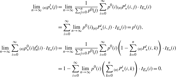 \begin{align*} \lim_{n\rightarrow \infty}{}_{(n)}p^t_{\ast}(j) & = \lim_{n\rightarrow\infty}\frac{1}{\sum_{j=0}^n p^0(j)}\sum_{i=0}^\infty p^0(i){}_{(n)}P^t_{\ast}(i,j)\cdot I_{E_n}(i) \\[5pt] & = \sum_{i=0}^\infty\lim_{n\rightarrow\infty}p^0(i){}_{(n)}P^t_{\ast}(i,j)\cdot I_{E_n}(i)=p^t(j), \\[5pt] \lim_{n\rightarrow\infty}\sum_{i=0}^\infty{}_{(n)}p^0_\ast(i)f_n^t(i)\cdot I_{E_n}(i) & = \lim_{n\rightarrow\infty}\frac{1}{\sum_{j=0}^n p^0(j)}\sum_{i=0}^\infty p^0(i) \Bigg(1-\sum_{k=0}^n{}_{(n)}P^t_{\ast}(i,k)\Bigg)\cdot I_{E_n}(i) \\[5pt] & = 1-\sum_{i=0}^\infty\lim_{n\rightarrow\infty}p^0(i)\Bigg(\sum_{k=0}^n{}_{(n)}P^t_{\ast}(i,k)\Bigg)\cdot I_{E_n}(i)=0. \end{align*}
Taking limits in n on both sides of (6), we obtain
![]() $\lim_{n\rightarrow \infty}{}_{(n,h)}p^t_{\ast}(j)=p^t(j)$
. This, together with the fact that
$\lim_{n\rightarrow \infty}{}_{(n,h)}p^t_{\ast}(j)=p^t(j)$
. This, together with the fact that
![]() $|a|=2a^+-a$
, where
$|a|=2a^+-a$
, where
![]() $a^+$
is the positive part of a, yields
$a^+$
is the positive part of a, yields
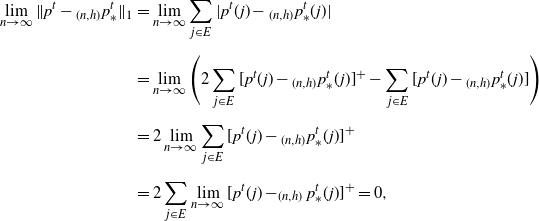 \begin{align*} \lim_{n\rightarrow\infty}\|p^t-{}_{(n,h)}p^t_{\ast}\|_1 & = \lim_{n\rightarrow\infty} \sum_{j\in E}|p^t(j)-{}{}_{(n,h)}p^t_{\ast}(j)| \\[5pt] & = \lim_{n\rightarrow\infty}\Bigg(2\sum_{j\in E}[p^t(j)-{}{}_{(n,h)}p^t_{\ast}(j)]^+ - \sum_{j\in E}[p^t(j)-{}{}_{(n,h)}p^t_{\ast}(j)]\Bigg) \\[5pt] & = 2\lim_{n\rightarrow \infty}\sum_{j\in E}[p^t(j)-{}{}_{(n,h)}p^t_{\ast}(j)]^+ \\[5pt] & = 2\sum_{j\in E}\lim_{n\rightarrow \infty}[p^t(j)-_{(n,h)}p^t_{\ast}(j)]^+=0, \end{align*}
where the penultimate equality follows from the dominated convergence theorem and the fact that
![]() $[p^t(j)-{}_{(n,h)}p^t_{\ast}(j)]^+ \leq p^t(j)$
and
$[p^t(j)-{}_{(n,h)}p^t_{\ast}(j)]^+ \leq p^t(j)$
and
![]() $\sum_{j\in E}p^t(j)=1$
. Using similar arguments also gives
$\sum_{j\in E}p^t(j)=1$
. Using similar arguments also gives
The next step is to figure out the limit of
![]() $\|{}_{(n,h)}\tilde{p}^t_{\ast}-{}{}_{(n,h)}p^t_{\ast}\|_1$
. Observe that
$\|{}_{(n,h)}\tilde{p}^t_{\ast}-{}{}_{(n,h)}p^t_{\ast}\|_1$
. Observe that
Let
Since
![]() ${}_{(n,h)}P^t$
is strongly ergodic for any n and Assumption 2 holds, it follows from Proposition 1 and Lemma 3 that
${}_{(n,h)}P^t$
is strongly ergodic for any n and Assumption 2 holds, it follows from Proposition 1 and Lemma 3 that
Note that we have, for
![]() $i\neq h$
,
$i\neq h$
,
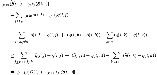 \begin{align*} & \|{}_{(n,h)}\tilde{Q}(i,\cdot) - {}_{(n,h)}Q(i,\cdot)\|_1 \\[5pt] & \qquad = \sum_{j\in E_n}|{}_{(n,h)}\tilde{q}(i,j)-{}_{(n,h)}q(i,j)| \\[5pt] & \qquad = \sum_{j\leq n,j\neq h}|\tilde{q}(i,j) - q(i,j)| + \Bigg|(\tilde{q}(i,h)-q(i,h)) + \sum_{k> n}(\tilde{q}(i,k)-q(i,k))\Bigg| \\[5pt] & \qquad \leq \sum_{j\leq n+1,j\neq h}|\tilde{q}(i,j)-q(i,j)| + \Bigg|(\tilde{q}(i,h)-q(i,h))+\sum_{k> n+1}(\tilde{q}(i,k)-q(i,k))\Bigg| \\[5pt] & \qquad = \|_{(n+1,h)}\tilde{Q}(i,\cdot) - _{(n+1,h)}Q(i,\cdot)\|_1, \end{align*}
and for
![]() $i=h$
,
$i=h$
,
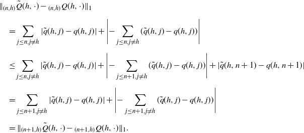 \begin{align*} & \|{}_{(n,h)}\tilde{Q}(h,\cdot) - {}_{(n,h)}Q(h,\cdot)\|_1 \\[5pt] & \quad = \sum_{j\leq n,j\neq h}|\tilde{q}(h,j)-q(h,j)| + \Bigg|{-}\sum_{j\leq n,j\neq h}(\tilde{q}(h,j)-q(h,j))\Bigg| \\[5pt] & \quad \leq \sum_{j\leq n,j\neq h}|\tilde{q}(h,j)-q(h,j)| + \Bigg|{-}\sum_{j\leq n+1,j\neq h}(\tilde{q}(h,j)-q(h,j))\Bigg| + |\tilde{q}(h,n+1)-q(h,n+1)| \\[5pt] & \quad = \sum_{j\leq n+1,j\neq h}|\tilde{q}(h,j)-q(h,j)| + \Bigg|{-}\sum_{j\leq n+1,j\neq h}(\tilde{q}(h,j)-q(h,j))\Bigg| \\[5pt] & \quad = \|_{(n+1,h)}\tilde{Q}(h,\cdot)-{}_{(n+1,h)}Q(h,\cdot)\|_1. \end{align*}
This, together with the assumption that V is nondecreasing, implies that both
![]() $\|{}_{(n)}\Delta\|_{1,V}$
and
$\|{}_{(n)}\Delta\|_{1,V}$
and
![]() $_{(n)}\tilde{p}^0(V_n)$
increase monotonously with n and
$_{(n)}\tilde{p}^0(V_n)$
increase monotonously with n and
![]() $\|_{(n)}\Delta\|_{1,V}\leq \|\Delta\|_{1,V}$
,
$\|_{(n)}\Delta\|_{1,V}\leq \|\Delta\|_{1,V}$
,
![]() $_{(n)}\kappa \leq \kappa$
. Applying the monotone convergence theorem gives
$_{(n)}\kappa \leq \kappa$
. Applying the monotone convergence theorem gives
![]() $\lim_{n\rightarrow \infty}\|_{(n)}\Delta\|_{1,V}=\|\Delta\|_{1,V}$
and
$\lim_{n\rightarrow \infty}\|_{(n)}\Delta\|_{1,V}=\|\Delta\|_{1,V}$
and
![]() $\lim_{n\rightarrow \infty}{}_{(n)}\kappa=\kappa$
. By this fact and (7), we have
$\lim_{n\rightarrow \infty}{}_{(n)}\kappa=\kappa$
. By this fact and (7), we have
Finally, we complete the proof by taking the limit of both sides of (5).
If
![]() $\tilde{P}$
has a stationary distribution, say
$\tilde{P}$
has a stationary distribution, say
![]() $\tilde{\pi}$
, as a consequence of the previous theorem, we can easily obtain a bound on the difference between
$\tilde{\pi}$
, as a consequence of the previous theorem, we can easily obtain a bound on the difference between
![]() $\pi$
and
$\pi$
and
![]() $\tilde{\pi}$
.
$\tilde{\pi}$
.
Corollary 1. Assume that the conditions in Theorem 1 hold. Then we have
where
![]() $\kappa'= \max\{\tilde{\pi}(V),{L}/{\delta}\}$
.
$\kappa'= \max\{\tilde{\pi}(V),{L}/{\delta}\}$
.
Proof. With
![]() $p^0=\pi$
,
$p^0=\pi$
,
![]() $\tilde{p}^0=\tilde{\pi}$
, and by letting
$\tilde{p}^0=\tilde{\pi}$
, and by letting
![]() $t\rightarrow \infty$
, we obtain the statement immediately by Theorem 1.
$t\rightarrow \infty$
, we obtain the statement immediately by Theorem 1.
3.3. Explicit results for particular CTMCs
Based on the technique of augmented truncations, our arguments inevitably require that
![]() ${}_{(n,h)}P^t$
uniformly satisfies Assumption 1, i.e. for any
${}_{(n,h)}P^t$
uniformly satisfies Assumption 1, i.e. for any
![]() $n\geq 1$
,
$n\geq 1$
,
![]() ${}_{(n,h)}P^t$
satisfies (3) for the same constants C and
${}_{(n,h)}P^t$
satisfies (3) for the same constants C and
![]() $\rho$
. There are two cases where we can easily verify this condition: CTMCs satisfying Doeblin conditions and stochastically monotone CTMCs. Explicit results for these two cases are given below.
$\rho$
. There are two cases where we can easily verify this condition: CTMCs satisfying Doeblin conditions and stochastically monotone CTMCs. Explicit results for these two cases are given below.
3.3.1. CTMCs satisfying Doeblin conditions
One of the most significant conditions for ergodicity of Markov chains is Doeblin’s condition. Q is said to satisfy the Doeblin condition if there exists a finite set
![]() $D \subseteq E$
satisfying
$D \subseteq E$
satisfying
![]() $\sum_{j\in D} q(i,j) \geq \alpha>0$
for all
$\sum_{j\in D} q(i,j) \geq \alpha>0$
for all
![]() $i \in T \;:\!=\; E \backslash D$
. It is worth noting that we can estimate the strongly ergodic rate if D is a single-point set [Reference Jacka and Roberts8, p. 913]. Here we give our proof.
$i \in T \;:\!=\; E \backslash D$
. It is worth noting that we can estimate the strongly ergodic rate if D is a single-point set [Reference Jacka and Roberts8, p. 913]. Here we give our proof.
Lemma 4. Suppose Q satisfies the Doeblin condition with single-point set
![]() $D=\{m\}$
and
$D=\{m\}$
and
![]() $\alpha>0$
. Then the CTMC X is strongly ergodic and
$\alpha>0$
. Then the CTMC X is strongly ergodic and
![]() $\|P^t(i,\cdot)-\pi\|_1\leq 2{\mathrm{e}}^{-\alpha t}$
.
$\|P^t(i,\cdot)-\pi\|_1\leq 2{\mathrm{e}}^{-\alpha t}$
.
Proof. Since
![]() $x > 1-{\mathrm{e}}^{-x}$
for any
$x > 1-{\mathrm{e}}^{-x}$
for any
![]() $x>0$
and
$x>0$
and
![]() $P^t(i,m)=q(i,m)t + o_i(t)$
, we have
$P^t(i,m)=q(i,m)t + o_i(t)$
, we have
For any
![]() $\varepsilon>0$
, there exists
$\varepsilon>0$
, there exists
![]() $t_0$
such that when
$t_0$
such that when
![]() $t<t_0$
,
$t<t_0$
,
![]() $|\inf_{i\neq m}o_i(t)|<\varepsilon$
and
$|\inf_{i\neq m}o_i(t)|<\varepsilon$
and
from which we can get
![]() $\inf_{i\neq m}P^t(i,m)\geq 1-{\mathrm{e}}^{-\alpha t}$
. In addition, we have
$\inf_{i\neq m}P^t(i,m)\geq 1-{\mathrm{e}}^{-\alpha t}$
. In addition, we have
![]() $P^t(m,m)\geq {\mathrm{e}}^{-q_i t}$
. Thus, we can choose small enough h such that
$P^t(m,m)\geq {\mathrm{e}}^{-q_i t}$
. Thus, we can choose small enough h such that
![]() $P^h(i,m)\geq 1-{\mathrm{e}}^{-\alpha h}$
for all
$P^h(i,m)\geq 1-{\mathrm{e}}^{-\alpha h}$
for all
![]() $i\in E$
. Then, for the h-skeleton chain with transition probabilities
$i\in E$
. Then, for the h-skeleton chain with transition probabilities
![]() $P^h(i,j)$
, we know from [Reference Meyn and Tweedie21, Theorem 16.2.4] that it is strongly ergodic and
$P^h(i,j)$
, we know from [Reference Meyn and Tweedie21, Theorem 16.2.4] that it is strongly ergodic and
For any
![]() $t \in \mathbb{R}_+$
with t of the form
$t \in \mathbb{R}_+$
with t of the form
![]() $t = nh + s$
for some
$t = nh + s$
for some
![]() $s \in [0, h)$
, we have
$s \in [0, h)$
, we have
Letting
![]() $h\rightarrow 0$
, the assertion follows immediately from the previous inequality and the fact that
$h\rightarrow 0$
, the assertion follows immediately from the previous inequality and the fact that
![]() $s\rightarrow 0$
as
$s\rightarrow 0$
as
![]() $h\rightarrow 0$
.
$h\rightarrow 0$
.
Theorem 1 and Lemma 4 lead to the following perturbation bounds for CTMCs satisfying Doeblin conditions.
Theorem 2. Let X be an irreducible CTMC on state space
![]() $E=\mathbb{Z}_+$
. Assume that Q satisfies the Doeblin condition with single-point set
$E=\mathbb{Z}_+$
. Assume that Q satisfies the Doeblin condition with single-point set
![]() $D=\{m\}$
and
$D=\{m\}$
and
![]() $\alpha>0$
. Suppose that Assumption 2 holds true for a nondecreasing function V. Then we have
$\alpha>0$
. Suppose that Assumption 2 holds true for a nondecreasing function V. Then we have
where
![]() $\kappa=\max\{\tilde{p}^0(V),{L}/{\delta}\}$
.
$\kappa=\max\{\tilde{p}^0(V),{L}/{\delta}\}$
.
Proof. Observe that if Q satisfies the Doeblin condition, then so does its augmented truncation
![]() ${}_{(n,h)}Q$
for any n such that
${}_{(n,h)}Q$
for any n such that
![]() $m\in E_n$
and
$m\in E_n$
and
![]() ${}{}_{(n,h)}q(i,m) \geq q(i,m) \geq \alpha$
for
${}{}_{(n,h)}q(i,m) \geq q(i,m) \geq \alpha$
for
![]() $i\in E_n$
and
$i\in E_n$
and
![]() $i\neq m$
. Due to this fact and Lemma 4, we can obtain the uniform convergence rate of
$i\neq m$
. Due to this fact and Lemma 4, we can obtain the uniform convergence rate of
![]() ${}_{(n,h)}Q$
, which is not smaller than
${}_{(n,h)}Q$
, which is not smaller than
![]() $\alpha$
. That is, we have
$\alpha$
. That is, we have
![]() $\|{}_{(n,h)}P^t(i,\cdot)-{}_{(n,h)}\pi\|_1\leq 2{\mathrm{e}}^{-\alpha t}$
. Then the assertion follows by Theorem 1 immediately.
$\|{}_{(n,h)}P^t(i,\cdot)-{}_{(n,h)}\pi\|_1\leq 2{\mathrm{e}}^{-\alpha t}$
. Then the assertion follows by Theorem 1 immediately.
We are now in a position to deal with our example of a linear birth and death process with catastrophes as described in Section 1. Note that Q, written as (1), evidently satisfies the Doeblin condition. For such a model, we will make a comparison of feasibility between the bounds in the V-norm and the weak norm, and show the quality of the latter.
Example 1. Consider a linear birth–death process with catastrophes on state space
![]() $E=\mathbb{Z}_+$
with q-matrix given by (1). Let
$E=\mathbb{Z}_+$
with q-matrix given by (1). Let
![]() $d=\inf_{i\geq 2} \{d_i,a\}>0$
. Now suppose that all the parameters are perturbed by the same amount
$d=\inf_{i\geq 2} \{d_i,a\}>0$
. Now suppose that all the parameters are perturbed by the same amount
![]() $\varepsilon$
, which implies Q is perturbed to be
$\varepsilon$
, which implies Q is perturbed to be
 \[ \tilde{Q}=\left( \begin{array}{c@{\quad}c@{\quad}c@{\quad}c@{\quad}c} -b-\varepsilon & b+\varepsilon & 0 & \cdots\\[5pt] a+\varepsilon & -(a+b+2\varepsilon) & b+\varepsilon & \cdots\\[5pt] d_2+\varepsilon & 2(a+\varepsilon) & -2(a+b+2\varepsilon)-d_2-\varepsilon & \cdots\\[5pt] \vdots & \vdots & \vdots & \ddots \end{array} \right), \]
and the perturbation matrix is given by (2).
Observe that
![]() $\inf_{i\geq 1}q_{i0}=d>0$
, which implies Q satisfies the Doeblin condition with single-point set
$\inf_{i\geq 1}q_{i0}=d>0$
, which implies Q satisfies the Doeblin condition with single-point set
![]() $D=\{0\}$
and
$D=\{0\}$
and
![]() $\alpha=d$
. Let
$\alpha=d$
. Let
![]() $\delta=({a-b})/{2}$
and
$\delta=({a-b})/{2}$
and
![]() $L=({a+b})/{2}+\varepsilon$
. Define the function V by
$L=({a+b})/{2}+\varepsilon$
. Define the function V by
![]() $V(i)=i+1$
,
$V(i)=i+1$
,
![]() $i\geq 0$
. It is easy to verify that
$i\geq 0$
. It is easy to verify that
![]() $\tilde{Q}V(i) \leq -\delta V(i)+L$
,
$\tilde{Q}V(i) \leq -\delta V(i)+L$
,
![]() $i \in E$
. From
$i \in E$
. From
 \[ \frac{\sum_{j}|\Delta(i,j)|}{V(i)} = \begin{cases} 2\varepsilon, & i=0,1, \\[5pt] \dfrac{4i+2}{i+1}\varepsilon, & i\geq 2, \end{cases} \qquad \frac{\sum_{j}|\Delta(i,j)|V(j)}{V(i)} = \begin{cases} 3\varepsilon, & i=0, \\[5pt] 4\varepsilon, & i=1, \\[5pt] \dfrac{4i^2+5i+2}{i+1}\varepsilon, & i \geq 2, \end{cases} \]
it follows that
This shows that the V-norm cannot be used to analyze this perturbation because
![]() $\|\Delta\|_V$
is always
$\|\Delta\|_V$
is always
![]() $\infty$
as the perturbation parameter
$\infty$
as the perturbation parameter
![]() $\varepsilon \rightarrow 0$
. However, letting
$\varepsilon \rightarrow 0$
. However, letting
by our Theorem 2 we have
![]() $\|\tilde{p}^t-p^t\|_1<2{\mathrm{e}}^{-dt}\|\tilde{p}^0-p^0\|_1+{8\kappa\varepsilon}/{d}$
.
$\|\tilde{p}^t-p^t\|_1<2{\mathrm{e}}^{-dt}\|\tilde{p}^0-p^0\|_1+{8\kappa\varepsilon}/{d}$
.
In addition, we give an simple example of a queuing model to demonstrate the applicability of our results.
Example 2. Consider an open Jackson network with two servers. We restrict ourselves here to the simplest assumptions: independent Poisson inputs with parameter
![]() $\lambda_i>0$
for
$\lambda_i>0$
for
![]() $i=1$
or 2, exponential service times with parameter
$i=1$
or 2, exponential service times with parameter
![]() $\mu_i>0$
, and first-in-first-out service discipline. Once a customer is served by server 1, they then join the queue at server 2. After they complete service at server 2, they are transferred with probability p to the end of the queue at server 1, and with probability
$\mu_i>0$
, and first-in-first-out service discipline. Once a customer is served by server 1, they then join the queue at server 2. After they complete service at server 2, they are transferred with probability p to the end of the queue at server 1, and with probability
![]() $1-p$
they leave the system. The whole system may experience a breakdown with exponential rate
$1-p$
they leave the system. The whole system may experience a breakdown with exponential rate
![]() $\mu_\mathrm{b}$
. If a breakdown occurs, all customers leave and the system immediately goes into repair. The repair time is also exponentially distributed with parameter
$\mu_\mathrm{b}$
. If a breakdown occurs, all customers leave and the system immediately goes into repair. The repair time is also exponentially distributed with parameter
![]() $\lambda_\mathrm{r}$
.
$\lambda_\mathrm{r}$
.
Denote by N the total number of customers in the system and by L the number of customers at server 1. Let us define the state by the pair (N, L). When the system is empty, it would not be enough to specify that there is no customer in the system (and hence at server 1) as we would also have to know whether the system is broken. So we introduce another state
![]() $(0,0,\mathrm{b})$
to indicate ‘empty due to breakdown’ and retain (0, 0) to represent ‘temporarily empty’ while the system is working. Let
$(0,0,\mathrm{b})$
to indicate ‘empty due to breakdown’ and retain (0, 0) to represent ‘temporarily empty’ while the system is working. Let
![]() $E^{k}=\{(k,i),0\leq i\leq k\}$
; then we are able to arrange the state space as
$E^{k}=\{(k,i),0\leq i\leq k\}$
; then we are able to arrange the state space as
![]() $E=\{(0,0,\mathrm{b}),E^{0},E^{1},\ldots\}$
. The generator Q can be expressed as
$E=\{(0,0,\mathrm{b}),E^{0},E^{1},\ldots\}$
. The generator Q can be expressed as
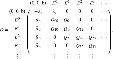
where
![]() $\vec{\mu}_\mathrm{b}$
is a column vector of all
$\vec{\mu}_\mathrm{b}$
is a column vector of all
![]() $\mu_\mathrm{b}$
s with appropriate length,
$\mu_\mathrm{b}$
s with appropriate length,
![]() $Q_{00}=-\lambda_1-\lambda_2-\mu_\mathrm{b}$
,
$Q_{00}=-\lambda_1-\lambda_2-\mu_\mathrm{b}$
,
![]() $Q_{01}=(\lambda_2,\lambda_1)$
, and, for
$Q_{01}=(\lambda_2,\lambda_1)$
, and, for
![]() $k\geq 1$
,
$k\geq 1$
,
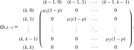
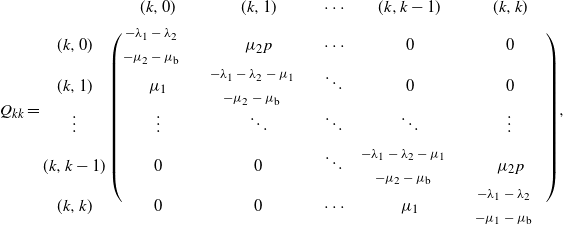
and

It is evident that Q satisfies the Doeblin condition with single-point set
![]() $D=\{0\}$
and
$D=\{0\}$
and
![]() $\alpha=\mu_\mathrm{b}$
. Suppose that the breakdown rate
$\alpha=\mu_\mathrm{b}$
. Suppose that the breakdown rate
![]() $\mu_\mathrm{b}$
is perturbed to be
$\mu_\mathrm{b}$
is perturbed to be
![]() $\mu_\mathrm{b}+\varepsilon$
and assume that
$\mu_\mathrm{b}+\varepsilon$
and assume that
Define a nondecreasing function V by
![]() $V(i,j)=\max\{s^{i+j},s^{2i-2}\}$
, where
$V(i,j)=\max\{s^{i+j},s^{2i-2}\}$
, where
We can check after some calculations that the perturbed continuous-time Markov chain satisfies the drift condition
![]() $\tilde{Q}V \leq -\delta V +L$
with
$\tilde{Q}V \leq -\delta V +L$
with
 \begin{align*} \delta & = (\lambda_1+\lambda_2+\mu_2 p)(1-s^2)+\omega (1-s^{-1})>0, \\[5pt] L & = c + \mu_\mathrm{b} + \varepsilon + \lambda_1(s^2-1)+\lambda_2(s-1). \end{align*}
Then it follows from Theorem 2 that
where
![]() $\kappa=\max\{\tilde{p}^0(V),{L}/{\delta}\}$
.
$\kappa=\max\{\tilde{p}^0(V),{L}/{\delta}\}$
.
3.3.2. CTMCs with monotone q-matrix
The chain X is said to be stochastically monotone if
![]() $\sum_{j\geq k}P^t(i,j)$
is a nondecreasing function of i for every fixed k and t. For an irreducible CTMC with regular q-matrix Q, the chain X is stochastically monotone if and only if Q is (stochastically) monotone, i.e.
$\sum_{j\geq k}P^t(i,j)$
is a nondecreasing function of i for every fixed k and t. For an irreducible CTMC with regular q-matrix Q, the chain X is stochastically monotone if and only if Q is (stochastically) monotone, i.e.
![]() $\sum_{j\geq k}q(i,j)\leq \sum_{j\geq k}q(m,j)$
, whenever
$\sum_{j\geq k}q(i,j)\leq \sum_{j\geq k}q(m,j)$
, whenever
![]() $i\leq m$
, and k is such that either
$i\leq m$
, and k is such that either
![]() $k\leq i$
or
$k\leq i$
or
![]() $k>m$
[Reference Anderson2]. Note that if Q is stochastically monotone, so is its last-column-augmented truncation
$k>m$
[Reference Anderson2]. Note that if Q is stochastically monotone, so is its last-column-augmented truncation
![]() $_{(n,n)}Q$
.
$_{(n,n)}Q$
.
We now introduce a drift condition that will be used frequently later.
Assumption 3. There exists a fixed state
![]() $m\in E$
and a bounded nonnegative function x such that
$m\in E$
and a bounded nonnegative function x such that
 \[ \left\{ \begin{array}{l@{\quad}l} Qx(i)\leq -1, & i\neq m,\\[5pt] x(i)=0, & i=m. \end{array} \right. \]
Considering the equivalence between the drift conditions, the following lemma is essentially the same as [Reference Liu, Zhang and Zhao16, Lemma 2.2], which presents the explicit uniform convergence rate for stochastically monotone CTMCs.
Lemma 5. If Q is monotone and satisfies Assumption 3, then, for any
![]() $t\geq 0$
,
$t\geq 0$
,
where
![]() $0<\beta\leq 1/(\sup_{i\in E}x(i)+1)$
.
$0<\beta\leq 1/(\sup_{i\in E}x(i)+1)$
.
Based on Theorem 1, Lemma 5, and the proof of Lemma 3, we can refine the perturbation bounds for stochastically monotone CTMCs.
Theorem 3. Let X be an irreducible and stochastically monotone CTMC on state space
![]() $E=\mathbb{Z}_+$
satisfying Assumption 3. Suppose that Assumption 2 holds true for a nondecreasing function V. Let
$E=\mathbb{Z}_+$
satisfying Assumption 3. Suppose that Assumption 2 holds true for a nondecreasing function V. Let
![]() $\kappa=\max\{\tilde{p}^0(V),{L}/{\delta}\}$
. Then
$\kappa=\max\{\tilde{p}^0(V),{L}/{\delta}\}$
. Then
 \begin{align*} \|\tilde{p}^t-p^t\|_{1} & \leq 4\bigg(\sup_{i\in E}x(i)+1\bigg)\exp\bigg\{{-}\bigg(\sup_{i\in E}x(i)+1\bigg)^{-1}t\bigg\} \|\tilde{p}^0-p^0\|_1 \\[5pt] & \quad + 4\bigg(\sup_{i\in E}x(i)+1\bigg)^2\kappa\|\Delta\|_{1,V}. \end{align*}
As an application, we adopt Theorem 3 to obtain the perturbation bounds for general birth and death processes. In particular instances, we further provide numerical analyses in terms of the relative errors.
Example 3. Let X be a birth–death process with q-matrix Q which is given by
![]() $q_{i,i+1}=b_i$
,
$q_{i,i+1}=b_i$
,
![]() $i\in \mathbb{Z}_+$
;
$i\in \mathbb{Z}_+$
;
![]() $q_{i,i-1}=a_i$
,
$q_{i,i-1}=a_i$
,
![]() $i\in \mathbb{N}$
;
$i\in \mathbb{N}$
;
![]() $q_{ij}=0$
,
$q_{ij}=0$
,
![]() $|i-j|\geq 2$
, where
$|i-j|\geq 2$
, where
![]() $a_i>0$
for
$a_i>0$
for
![]() $i\in \mathbb{N}$
and
$i\in \mathbb{N}$
and
![]() $b_i>0$
for
$b_i>0$
for
![]() $i\in \mathbb{Z}_+$
. It is well known that Q is regular if and only if Q is conservative and
$i\in \mathbb{Z}_+$
. It is well known that Q is regular if and only if Q is conservative and
It is easy to check that Q is stochastically monotone and so is X. From [Reference Zhang28], we know that the function x defined by
 \begin{equation*} x(0) = 0, \qquad x(i) = \sum_{k=0}^{i-1}\Bigg(\frac{1}{a_{k+1}}+\sum_{j=k+1}^\infty\frac{b_{k+1}\cdots b_j}{a_{k+1}\cdots a_{j+1}}\Bigg), \quad i\geq 1, \end{equation*}
satisfies Assumption 3 with equality. Obviously, x(i) is strictly increasing and
 \[ \sup_{i\in E}x(i) = \sum_{k=0}^\infty\Bigg(\frac{1}{a_{k+1}} + \sum_{j=k+1}^\infty\frac{b_{k+1}\cdots b_j}{a_{k+1}\cdots a_{j+1}}\Bigg) \;:\!=\; A. \]
Then from Theorem 3 we have the following statement.
Let X be a birth–death process with regular q-matrix Q. Suppose that
![]() $A<\infty$
and Assumption 2 holds for a nondecreasing function V. Then
$A<\infty$
and Assumption 2 holds for a nondecreasing function V. Then
where
![]() $\kappa=\max\{\tilde{p}^0(V),{L}/{\delta}\}$
.
$\kappa=\max\{\tilde{p}^0(V),{L}/{\delta}\}$
.
To present a numerical illustration of our results, we further consider the special case
![]() $b_0=1$
and
$b_0=1$
and
![]() $a_i=b_i=s^i$
,
$a_i=b_i=s^i$
,
![]() $i\geq 1$
. Suppose that the birth and death rates are perturbed to be
$i\geq 1$
. Suppose that the birth and death rates are perturbed to be
![]() $b_0=1+\varepsilon$
and
$b_0=1+\varepsilon$
and
![]() $a_i=b_i=s^i+\varepsilon$
for
$a_i=b_i=s^i+\varepsilon$
for
![]() $i\geq 1$
. By simple calculations, we have
$i\geq 1$
. By simple calculations, we have
![]() $A={s}/{(s-1)^2}$
,
$A={s}/{(s-1)^2}$
,
 \[ \pi(i) = \pi(0)\frac{1}{s^i}, \qquad \tilde{\pi}(i) = \pi(0)\prod_{k=1}^i\frac{s^{k-1}+\varepsilon}{s^k+\varepsilon}. \]
Take
![]() $V\equiv 1$
and note that Assumption 2 is satisfied with
$V\equiv 1$
and note that Assumption 2 is satisfied with
![]() $L=\delta>0$
. In view of (8), we can bound
$L=\delta>0$
. In view of (8), we can bound
![]() $\|\tilde{\pi}-\pi\|_1$
with
$\|\tilde{\pi}-\pi\|_1$
with
![]() $\tilde{p}^0=p^0$
and by letting
$\tilde{p}^0=p^0$
and by letting
![]() $t\rightarrow \infty$
. It follows that
$t\rightarrow \infty$
. It follows that
For
![]() $U(\epsilon)$
to become informative,
$U(\epsilon)$
to become informative,
![]() $\varepsilon$
has to be smaller than
$\varepsilon$
has to be smaller than
![]() $0.0599$
for
$0.0599$
for
![]() $s = 4$
, as otherwise
$s = 4$
, as otherwise
![]() $U(\varepsilon)$
becomes larger than 2. It can be seen that the perturbation bound
$U(\varepsilon)$
becomes larger than 2. It can be seen that the perturbation bound
![]() $U(\varepsilon)$
diminishes linearly as
$U(\varepsilon)$
diminishes linearly as
![]() $\varepsilon$
tends to 0.
$\varepsilon$
tends to 0.
To test the performance of
![]() $U(\varepsilon)$
, we investigate the relative error of the perturbation bound, which was first introduced and discussed in [Reference Abbas, Berkhout and Heidergott1] and is given by
$U(\varepsilon)$
, we investigate the relative error of the perturbation bound, which was first introduced and discussed in [Reference Abbas, Berkhout and Heidergott1] and is given by
Clearly, a smaller relative error means a sharper bound. In the setting of
![]() $s=4$
, the relative errors of
$s=4$
, the relative errors of
![]() $U(\varepsilon)$
are plotted in Figure 1, which shows that the relative error of the condition number bound
$U(\varepsilon)$
are plotted in Figure 1, which shows that the relative error of the condition number bound
![]() $U(\varepsilon)$
converges to a finite non-zero value as
$U(\varepsilon)$
converges to a finite non-zero value as
![]() $\varepsilon \rightarrow 0$
, which is consistent with the findings of [Reference Abbas, Berkhout and Heidergott1]. Hence, we have to acknowledge that our results might not be that sharp due to the limitations inherent in the arguments of condition number bounds.
$\varepsilon \rightarrow 0$
, which is consistent with the findings of [Reference Abbas, Berkhout and Heidergott1]. Hence, we have to acknowledge that our results might not be that sharp due to the limitations inherent in the arguments of condition number bounds.
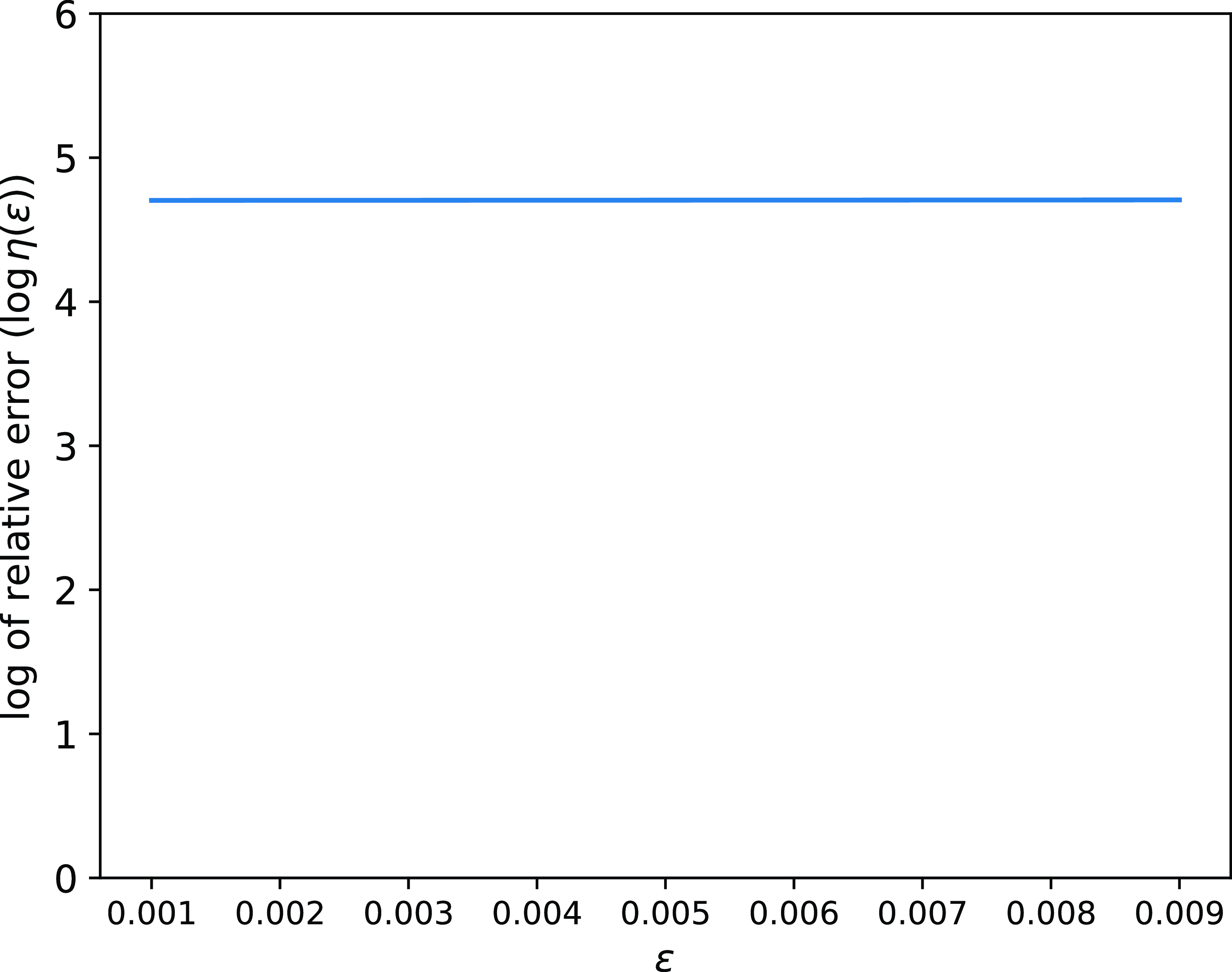
Figure 1. Log relative errors
![]() $\log(\eta(\varepsilon))$
for
$\log(\eta(\varepsilon))$
for
![]() $\|\tilde{\pi}-\pi\|_1$
with
$\|\tilde{\pi}-\pi\|_1$
with
![]() $\varepsilon \in (0,0.01]$
in the case of
$\varepsilon \in (0,0.01]$
in the case of
![]() $s=4$
.
$s=4$
.
4. Perturbation analysis for exponentially ergodic CTMCs
By using similar arguments to Section 3 but with the introduction of multiplicative decomposition, we derive perturbation bounds for exponentially ergodic CTMCs. In particular, estimates for stochastically monotone CTMCs are proposed.
In this part, the following assumptions are considered.
Assumption 4.
![]() $P^t$
is V-uniformly ergodic with positive constants
$P^t$
is V-uniformly ergodic with positive constants
![]() $\rho <1$
and
$\rho <1$
and
![]() $C < \infty$
and finite function V.
$C < \infty$
and finite function V.
Assumption 5. There is a constant
![]() $M<\infty$
such that
$M<\infty$
such that
4.1. Finite state spaces
First, we have the following perturbation bounds for exponentially ergodic CTMCs on a finite state space
![]() $E_n$
.
$E_n$
.
Proposition 2. Let X be an irreducible CTMC on finite state space
![]() $E_n$
. Suppose that Assumptions 2, 4, and 5 hold for the same function V. Then, for
$E_n$
. Suppose that Assumptions 2, 4, and 5 hold for the same function V. Then, for
![]() $\|\Delta\|_{1,V}\in(0,1/{\mathrm{e}})$
we have
$\|\Delta\|_{1,V}\in(0,1/{\mathrm{e}})$
we have
where
![]() $\kappa=\max\{\tilde{p}^0(V),{L}/{\delta}\}$
.
$\kappa=\max\{\tilde{p}^0(V),{L}/{\delta}\}$
.
Proof. In the proof of Proposition 1, we obtained
 \begin{align*} \|(\tilde{p}^0-p^0)P^t\|_1 & \leq \|(\tilde{p}^0-p^0)P^t\|_V \leq \|\tilde{p}^0-p^0\|_V\cdot\tau_V(P^t) \leq C\rho^t\|\tilde{p}^0-p^0\|_V, \\[5pt] \|\tilde{p}^{t-u}(\tilde{Q}-Q)P^u\|_{V} & \leq \|\tilde{p}^{t-u}(\tilde{Q}-Q)\|_{V}\tau_{V}(P^u). \end{align*}
Fix a real number
![]() $r\in (0,1)$
and let
$r\in (0,1)$
and let
![]() $s=1-r$
. By considering the definition of
$s=1-r$
. By considering the definition of
![]() $\tau_1(P^u)$
, we can see that
$\tau_1(P^u)$
, we can see that
![]() $\tau_1(P^u)\leq 1$
. These lead to
$\tau_1(P^u)\leq 1$
. These lead to
 \begin{align*} \|\tilde{p}^{t-u}(\tilde{Q}-Q)P^u\|_1 & \leq \big\|\tilde{p}^{t-u}(\tilde{Q}-Q)P^u\big\|_1^r\big\|\tilde{p}^{t-u}(\tilde{Q}-Q)P^u\big\|_{V}^s \\[5pt] & \leq \big\|\tilde{p}^{t-u}(\tilde{Q}-Q)\big\|_1^r(\tau_1(P^u))^r \big\|\tilde{p}^{t-u}(\tilde{Q}-Q)\big\|_{V}^s(\tau_{V}(P^u))^s \\[5pt] & \leq \big\|\tilde{p}^{t-u}(\tilde{Q}-Q)\big\|_1^r\big\|\tilde{p}^{t-u}(\tilde{Q}-Q)\big\|_{V}^s(\tau_{V}(P^u))^s. \end{align*}
Further, we also have
 \begin{align*} \|\tilde{p}^{t-u}(\tilde{Q}-Q)\|_1 & \leq \sum_{i\in E_n}\tilde{p}^{t-u}(i)\|\tilde{Q}(i,\cdot)-Q(i,\cdot)\|_1 \leq \|\Delta\|_{1,V}\sum_{i\in E_n} \tilde{p}^{t-u}(i)V(i), \\[5pt] \|\tilde{p}^{t-u}(\tilde{Q}-Q)\|_{V} & \leq \sum_{i\in E_n}\tilde{p}^{t-u}(i)\|\tilde{Q}(i,\cdot)-Q(i,\cdot)\|_{V} \leq M\sum_{i\in E_n} \tilde{p}^{t-u}(i)V(i). \end{align*}
From the proof of the inequality (4) and the drift condition in Assumption 2, we have, for
![]() $t-u\geq 0$
,
$t-u\geq 0$
,
Then we get
Finally, it follows from Lemma 2 that
and hence
For
![]() $\|\Delta\|_{1,V}\in (0,1/{\mathrm{e}})$
, we can choose the numbers
$\|\Delta\|_{1,V}\in (0,1/{\mathrm{e}})$
, we can choose the numbers
![]() $r=1+(\log\|\Delta\|_{1,V})^{-1}$
and
$r=1+(\log\|\Delta\|_{1,V})^{-1}$
and
![]() $s=-(\log\|\Delta\|_{1,V})^{-1}$
, which leads to
$s=-(\log\|\Delta\|_{1,V})^{-1}$
, which leads to
![]() $\big\|\Delta\big\|_{1,V}^r={\mathrm{e}}\|\Delta\|_{1,V}$
and allows us to complete the proof.
$\big\|\Delta\big\|_{1,V}^r={\mathrm{e}}\|\Delta\|_{1,V}$
and allows us to complete the proof.
Remark 2. This result parallels [Reference Rudolf and Schweizer26, Theorem 3.2] for DTMCs, which can also be derived through the uniformization technique.
4.2. Infinitely countable state spaces
By the technique of augmented truncations used in Section 3, we can get our results for exponentially ergodic CTMCs on an infinitely countable state space.
Theorem 4. Let X be an irreducible CTMC on state space
![]() $E=\mathbb{Z}_+$
, and
$E=\mathbb{Z}_+$
, and
![]() $V\colon E\rightarrow[1,\infty)$
a nondecreasing function. For a large enough integer N such that
$V\colon E\rightarrow[1,\infty)$
a nondecreasing function. For a large enough integer N such that
![]() $N\geq h$
, assume that
$N\geq h$
, assume that
![]() $\{{}_{(n,h)}P^t,n\geq N\}$
uniformly satisfies Assumption 4 with
$\{{}_{(n,h)}P^t,n\geq N\}$
uniformly satisfies Assumption 4 with
![]() $V_n$
, i.e. there exist positive constants
$V_n$
, i.e. there exist positive constants
![]() $\rho <1$
and
$\rho <1$
and
![]() $C < \infty$
such that, for any i, t, and
$C < \infty$
such that, for any i, t, and
![]() $n\geq N$
,
$n\geq N$
,
Moreover, suppose that Assumptions 2 and 5 hold for V. Then, for
![]() $\|\Delta\|_{1,V} \in (0,1/{\mathrm{e}})$
,
$\|\Delta\|_{1,V} \in (0,1/{\mathrm{e}})$
,
where
![]() $\kappa=\max\{\tilde{p}^0(V),{L}/{\delta}\}$
.
$\kappa=\max\{\tilde{p}^0(V),{L}/{\delta}\}$
.
Proof. Referring to the proof of Theorem 1, we know that
and
![]() $\lim_{n\rightarrow\infty}\|p^t-{}_{(n,h)}p_{\ast}^t\|_1=0$
,
$\lim_{n\rightarrow\infty}\|p^t-{}_{(n,h)}p_{\ast}^t\|_1=0$
,
![]() $\lim_{n\rightarrow\infty}\|\tilde{p}^t-{}_{(n,h)}\tilde{p}_{\ast}^t\|_1=0$
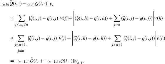
. Since V is nondecreasing, we can see that, for
$\lim_{n\rightarrow\infty}\|\tilde{p}^t-{}_{(n,h)}\tilde{p}_{\ast}^t\|_1=0$
. Since V is nondecreasing, we can see that, for
![]() $i\neq h$
,
$i\neq h$
,
 \begin{align*} \|{}_{(n,h)} &\tilde{Q}(i,\cdot)-{}_{(n,h)}Q(i,\cdot)\|_{V_n} \\[5pt] & = \sum_{j\leq n,j\neq h}|\tilde{q}(i,j)-q(i,j)|V(j) + \Bigg|(\tilde{q}(i,h)-q(i,h))+\sum_{j>n}(\tilde{q}(i,j)-q(i,j))\Bigg|V(h) \\[5pt] & \leq \sum_{\substack{j\leq n+1,\\[5pt] j\neq h}}|\tilde{q}(i,j)-q(i,j)|V(j) + \Bigg|(\tilde{q}(i,h)-q(i,h))+\sum_{j>n+1}(\tilde{q}(i,j)-q(i,j))\Bigg|V(h) \\[5pt] & = \|_{(n+1,h)}\tilde{Q}(i,\cdot)-{}_{(n+1,h)}Q(i,\cdot)\|_{V_{n+1}}, \end{align*}
and for
![]() $i=h$
,
$i=h$
,
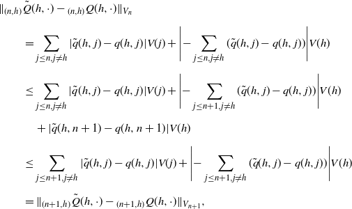 \begin{align*} \|{}_{(n,h)} &\tilde{Q}(h,\cdot)-{}_{(n,h)}Q(h,\cdot)\| _{V_n} \\[5pt] & = \sum_{j\leq n,j\neq h}|\tilde{q}(h,j)-q(h,j)|V(j) + \Bigg|{-}\sum_{j\leq n,j\neq h}(\tilde{q}(h,j)-q(h,j))\Bigg|V(h) \\[5pt] & \leq \sum_{j\leq n,j\neq h}|\tilde{q}(h,j)-q(h,j)|V(j) + \Bigg|{-}\sum_{j\leq n+1, j\neq h}(\tilde{q}(h,j)-q(h,j))\Bigg|V(h) \\[5pt] & \quad + |\tilde{q}(h,n+1)-q(h,n+1)|V(h) \\[5pt] & \leq \sum_{j\leq n+1,j\neq h}|\tilde{q}(h,j)-q(h,j)|V(j) + \Bigg|{-}\sum_{j\leq n+1,j\neq h}(\tilde{q}(h,j)-q(h,j))\Bigg|V(h) \\[5pt] & = \|_{(n+1,h)}\tilde{Q}(h,\cdot)-{}_{(n+1,h)}Q(h,\cdot)\|_{V_{n+1}}, \end{align*}
which implies
Let
![]() $\|_{(n)}\Delta\|_{1,V}=\sup_{i\in E_n}{\|{}_{(n,h)}\tilde{Q}(i,\cdot)-{}_{(n,h)}Q(i,\cdot)\|_{1}}/{V(i)}$
and
$\|_{(n)}\Delta\|_{1,V}=\sup_{i\in E_n}{\|{}_{(n,h)}\tilde{Q}(i,\cdot)-{}_{(n,h)}Q(i,\cdot)\|_{1}}/{V(i)}$
and
![]() $_{(n)}\kappa=\max\{{}_{(n)}\tilde{p}^0(V_n),{L}/{\delta}\}$
. Since
$_{(n)}\kappa=\max\{{}_{(n)}\tilde{p}^0(V_n),{L}/{\delta}\}$
. Since
![]() ${}_{(n,h)}P^t$
uniformly satisfies V-uniform ergodicity and Assumption 2 holds true for V, it follows from Lemma 3 and Proposition 2 that, for
${}_{(n,h)}P^t$
uniformly satisfies V-uniform ergodicity and Assumption 2 holds true for V, it follows from Lemma 3 and Proposition 2 that, for
![]() $\|_{(n)}\Delta\|_{1,V} \in (0,1/{\mathrm{e}})$
,
$\|_{(n)}\Delta\|_{1,V} \in (0,1/{\mathrm{e}})$
,
 \begin{align*} \|{}_{(n,h)}\tilde{p}^t-{}_{(n,h)}p^t\|_{1} &\leq C\rho^t\|_{(n)}\tilde{p}^0-{}_{(n)}p^0\|_{V_n} \\[5pt] &\quad + \frac{{\mathrm{e}}{}_{(n)}\kappa \|{}_{(n)}\Delta\|_{1,V} }{\log\rho}(CM)^{-(\log\|{}_{(n)}\Delta\|_{1,V})^{-1}} \log\|{}_{(n)}\Delta\|_{1,V}. \end{align*}
Using similar arguments to the proof of Theorem 1 gives
![]() $\lim_{n\rightarrow\infty}\|{}_{(n)}\Delta\|_{1,V}=\|\Delta\|_{1,V}$
,
$\lim_{n\rightarrow\infty}\|{}_{(n)}\Delta\|_{1,V}=\|\Delta\|_{1,V}$
,
![]() $\lim_{n\rightarrow \infty}{}_{(n)}\kappa=\kappa$
, and
$\lim_{n\rightarrow \infty}{}_{(n)}\kappa=\kappa$
, and
![]() $\lim_{n\rightarrow \infty}\|_{(n)}\tilde{p}^0-_{(n)}p^0\|_{V_n}=\|\tilde{p}^0-p^0\|_V$
. Hence, for
$\lim_{n\rightarrow \infty}\|_{(n)}\tilde{p}^0-_{(n)}p^0\|_{V_n}=\|\tilde{p}^0-p^0\|_V$
. Hence, for
![]() $\|\Delta\|_{1,V} \in (0,1/{\mathrm{e}})$
we have
$\|\Delta\|_{1,V} \in (0,1/{\mathrm{e}})$
we have
By taking the limit of both sides of (9), we obtain the assertion immediately.
As a consequence of the previous theorem, we have the following results on the distance between the two stationary distributions
![]() $\tilde{\pi}$
and
$\tilde{\pi}$
and
![]() $\pi$
.
$\pi$
.
Corollary 2. Assume that the conditions in Theorem 4 hold. Then, for
![]() $\|\Delta\|_{1,V} \in (0,1/{\mathrm{e}})$
,
$\|\Delta\|_{1,V} \in (0,1/{\mathrm{e}})$
,
where
![]() $\kappa'=\max\{\tilde{\pi}(V),{L}/{\delta}\}$
.
$\kappa'=\max\{\tilde{\pi}(V),{L}/{\delta}\}$
.
4.3. Explicit results for CTMCs with monotone q-matrix
For a class of exponentially ergodic CTMCs, the condition in Theorem 4 that
![]() ${}_{(n,h)}P^t$
uniformly satisfies Assumption 4 is easy to verify. In the remainder of this part, we give explicit results for stochastically monotone CTMCs that satisfy the following drift condition.
${}_{(n,h)}P^t$
uniformly satisfies Assumption 4 is easy to verify. In the remainder of this part, we give explicit results for stochastically monotone CTMCs that satisfy the following drift condition.
Assumption 6. There exists a nondecreasing function
![]() $V\colon E\rightarrow [1,\infty)$
and positive constants c and
$V\colon E\rightarrow [1,\infty)$
and positive constants c and
![]() $K<\infty$
such that
$K<\infty$
such that
![]() $QV(i) \leq -cV(i)+K\cdot I_{\{0\}}(i)$
.
$QV(i) \leq -cV(i)+K\cdot I_{\{0\}}(i)$
.
Based on this drift condition, [Reference Lund, Meyn and Tweedie17] proposed an exponential convergence rate for stochastically monotone CTMCs.
Lemma 6. Suppose that X is an irreducible and stochastically monotone CTMC on the state space
![]() $E=\mathbb{Z}_+$
satisfying Assumption 6. Then
$E=\mathbb{Z}_+$
satisfying Assumption 6. Then
As an immediate consequence of Lemma 6 and Theorem 4, we obtain the following theorem.
Theorem 5. Let X be an irreducible and stochastically monotone CTMC on the state space
![]() $E=\mathbb{Z}_+$
satisfying Assumption 6. Moreover, suppose that Assumptions 2 and 5 hold for the nondecreasing function V. Then, for
$E=\mathbb{Z}_+$
satisfying Assumption 6. Moreover, suppose that Assumptions 2 and 5 hold for the nondecreasing function V. Then, for
![]() $\|\Delta\|_{1,V} \in (0,1/{\mathrm{e}})$
,
$\|\Delta\|_{1,V} \in (0,1/{\mathrm{e}})$
,
 \begin{multline*} \|\tilde{p}^t-p^t\|_{1} \leq 2\bigg(1+\frac{K}{c}\cdot\frac{1}{\inf_{i\in E}V(i)}\bigg){\mathrm{e}}^{-ct} \|\tilde{p}^0-p^0\|_V \\ + \frac{{\mathrm{e}}\kappa\|\Delta\|_{1,V}}{-c} \bigg[2M\bigg(1+\frac{K}{c}\cdot\frac{1}{\inf_{i\in E}V(i)}\bigg)\bigg]^{-(\log\|\Delta\|_{1,V})^{-1}} \log\|\Delta\|_{1,V}, \end{multline*}
where
![]() $\kappa=\max\{\tilde{p}^0(V),{L}/{\delta}\}$
.
$\kappa=\max\{\tilde{p}^0(V),{L}/{\delta}\}$
.
Proof. Note that if Q is stochastically monotone, so is its
![]() $(n+1)\times(n+1)$
northwest corner truncation
$(n+1)\times(n+1)$
northwest corner truncation
![]() $_{(n,n)}Q$
augmented in the last column. Since V is nondecreasing, it follows from the proof of Lemma 3 that
$_{(n,n)}Q$
augmented in the last column. Since V is nondecreasing, it follows from the proof of Lemma 3 that
![]() $_{(n,n)}Q$
uniformly satisfies the conditions of Lemma 6 with
$_{(n,n)}Q$
uniformly satisfies the conditions of Lemma 6 with
![]() $V_n$
, and
$V_n$
, and
 \begin{align*} \|_{(n,n)}P^t(i,\cdot)-{}_{(n,n)}\pi\|_{V_n} & \leq 2{\mathrm{e}}^{-ct}\bigg[V_n(i)(1-I_{\{0\}}(i))+\frac{K}{c}\bigg] \\[5pt] & \leq 2\bigg(1+\frac{K}{c}\cdot\frac{1}{\inf_{i\in E}V(i)}\bigg)V_n(i){\mathrm{e}}^{-ct}. \end{align*}
By taking
![]() $h=n$
and using similar arguments to the proof of Theorem 4, we can obtain the statement immediately.
$h=n$
and using similar arguments to the proof of Theorem 4, we can obtain the statement immediately.
In the following, we show, through an example of birth and death processes with catastrophes, that our results in the weak sense are more feasible than V-normwise bounds in some cases.
Example 4. Consider a birth–death process with catastrophes on the state space
![]() $E=\mathbb{Z}_+$
with q-matrix
$E=\mathbb{Z}_+$
with q-matrix
 \[ Q=\left( \begin{array}{c@{\quad}c@{\quad}c@{\quad}c@{\quad}c} -b & b & 0 &0 & \cdots\\[5pt] a+\varepsilon & -(a+b+\varepsilon) & b & 0 & \cdots\\[5pt] d_2+\varepsilon & 2a & -2(a+b)-d_2-\varepsilon & 2b & \cdots\\[5pt] d_3+\varepsilon & 0 & 3a & -3(a+b)-d_3-\varepsilon & \cdots\\[5pt] \vdots & \vdots & \vdots & \vdots & \ddots \end{array} \right), \]
where
![]() $d_i$
,
$d_i$
,
![]() $i\geq 2$
, is a nonnegative decreasing sequence and a, b,
$i\geq 2$
, is a nonnegative decreasing sequence and a, b,
![]() $\varepsilon$
are positive constants such that
$\varepsilon$
are positive constants such that
![]() $a>\max\{b,d_2\}$
. Suppose the q-matrix is perturbed to be
$a>\max\{b,d_2\}$
. Suppose the q-matrix is perturbed to be
 \[ \tilde{Q}= \left( \begin{array}{c@{\quad}c@{\quad}c@{\quad}c@{\quad}c} -b & b & 0 & 0 & \cdots\\[5pt] a & -(a+b) & b & 0 & \cdots\\[5pt] d_2 & 2a & -2(a+b)-d_2 & 2b & \cdots\\[5pt] d_3 & 0 & 3a & -3(a+b)-d_3 & \cdots\\[5pt] \vdots & \vdots & \vdots & \vdots & \ddots \end{array} \right). \]
It is obvious that Q is monotone. Define the function V by
![]() $V(i)=1+({i+1})/{\varepsilon}$
,
$V(i)=1+({i+1})/{\varepsilon}$
,
![]() $i\geq 0$
. Then we can easily verify that
$i\geq 0$
. Then we can easily verify that
Let
To use [Reference Liu14, Theorem 3.3], we only need to check that
![]() $\|\Delta\|_V<{c}/({1+\pi(V)})$
or
$\|\Delta\|_V<{c}/({1+\pi(V)})$
or
![]() $\|\Delta\|_V<{c^2}/({K+c})$
. Observe that
$\|\Delta\|_V<{c^2}/({K+c})$
. Observe that
![]() $M=\|\Delta\|_V=({2\varepsilon^2+3\varepsilon})/({\varepsilon+2}) \rightarrow 0$
as
$M=\|\Delta\|_V=({2\varepsilon^2+3\varepsilon})/({\varepsilon+2}) \rightarrow 0$
as
![]() $\varepsilon \rightarrow 0$
. Unfortunately, when
$\varepsilon \rightarrow 0$
. Unfortunately, when
![]() $a-b<\min\{3,\sqrt{3(a+b)}\}$
, we can get
$a-b<\min\{3,\sqrt{3(a+b)}\}$
, we can get
 \begin{align*} \frac{c}{1+\pi(V)} < \frac{c}{1+(1+{1}/{\varepsilon})} = \frac{1}{\varepsilon+2}\cdot\frac{(a-b)\varepsilon}{2\varepsilon+1} < \frac{2\varepsilon^2+3\varepsilon}{\varepsilon+2} & = \|\Delta\|_V, \\[5pt] \frac{c^2}{K+c} = \frac{c}{({K}/{c})+1} = \frac{1}{\varepsilon+2}\cdot\frac{a-b}{({K}/{c})+1} < \frac{2\varepsilon^2+3\varepsilon}{\varepsilon+2} & = \|\Delta\|_V. \end{align*}
Hence, in the case where
![]() $a-b<\min\{3,\sqrt{3(a+b)}\}$
, the condition cannot be satisfied and the results of [Reference Liu14, Theorem 3.3] fail.
$a-b<\min\{3,\sqrt{3(a+b)}\}$
, the condition cannot be satisfied and the results of [Reference Liu14, Theorem 3.3] fail.
However, our results in the weak sense are still valid for such a case. For the same function V, we can also see that
![]() $\tilde{Q} V(i) \leq -c V(i) + K$
,
$\tilde{Q} V(i) \leq -c V(i) + K$
,
![]() $i\in E$
. To use our Theorem 5, we only require that
$i\in E$
. To use our Theorem 5, we only require that
Therefore, if
![]() $\varepsilon$
is small enough, the condition will be satisfied and we can obtain
$\varepsilon$
is small enough, the condition will be satisfied and we can obtain
 \begin{align} \|\tilde{p}^t-p^t\|_1 & \leq 2\bigg(1+\frac{a\varepsilon+a+b}{(a-b)(\varepsilon+1)}\bigg) \exp\bigg\{{-}\frac{a-b}{\varepsilon+2}t\bigg\} \nonumber \\[5pt] & \quad - \frac{2\varepsilon^2{\mathrm{e}}\kappa'}{a-b}\log\bigg[\frac{2\varepsilon^2}{\varepsilon+2}\bigg] \bigg\{\frac{4\varepsilon^2+6\varepsilon}{\varepsilon+2} \bigg(1+\frac{a\varepsilon+a+b}{(a-b)(\varepsilon+1)}\bigg)\bigg\}^{-(\log({2\varepsilon^2}/({\varepsilon+2})))^{-1}}, \end{align}
where
Obviously, the second term on the right-hand side of (10) is
This shows that the weak norm is a better choice than the V-norm to analyze the perturbation for this example, and our bounds are more feasible than the bounds in [Reference Liu14].
5. Conclusion
By the technique of augmented truncations, we obtained accurate bounds on
![]() $\|\tilde{p}^t-p^t\|_1$
in terms of the convergence rate and drift condition for strongly and exponentially ergodic CTMCs, respectively. In particular, the explicit results were derived for CTMCs satisfying Doeblin or stochastically monotone conditions. Through some examples, we showed that when the perturbation matrices are unbounded, the V-normwise bounds may fail while our bounds in the weak norm still hold. We now discuss possible extensions and improvements of the results in this paper.
$\|\tilde{p}^t-p^t\|_1$
in terms of the convergence rate and drift condition for strongly and exponentially ergodic CTMCs, respectively. In particular, the explicit results were derived for CTMCs satisfying Doeblin or stochastically monotone conditions. Through some examples, we showed that when the perturbation matrices are unbounded, the V-normwise bounds may fail while our bounds in the weak norm still hold. We now discuss possible extensions and improvements of the results in this paper.
In Theorems 1 and 4, it is required that
![]() $_{(n,h)}P^t$
has a uniform convergence rate, which may be difficult to verify for general CTMCs. We may expect a more straightforward condition on
$_{(n,h)}P^t$
has a uniform convergence rate, which may be difficult to verify for general CTMCs. We may expect a more straightforward condition on
![]() $P^t$
rather than
$P^t$
rather than
![]() $_{(n,h)}P^t$
. However, our arguments with the approach of augmented truncations fail to do that. It may be interesting to investigate this in different ways.
$_{(n,h)}P^t$
. However, our arguments with the approach of augmented truncations fail to do that. It may be interesting to investigate this in different ways.
Observe that for exponentially ergodic CTMCs, our bounds rely on the boundedness of
![]() $\|\Delta\|_V$
. When the perturbation matrix is unbounded, this condition cannot be satisfied and the bounds given in Section 4 may fail to hold. To investigate this issue requires some different methods, which is a topic for future research.
$\|\Delta\|_V$
. When the perturbation matrix is unbounded, this condition cannot be satisfied and the bounds given in Section 4 may fail to hold. To investigate this issue requires some different methods, which is a topic for future research.
Following [Reference Abbas, Berkhout and Heidergott1], the perturbation bounds we presented are condition number bounds. Example 3 illustrates that the relative error of our bound converges to a finite non-zero value as the perturbation size
![]() $\varepsilon \rightarrow 0$
. It is open to find a good way to derive bounds in the weak sense whose relative error vanishes.
$\varepsilon \rightarrow 0$
. It is open to find a good way to derive bounds in the weak sense whose relative error vanishes.
One possible extension is to consider a perturbation for a continuous-time Markov process on a continuous state space, say
![]() $[0,\infty)$
. To the best of our knowledge, this is a quite new topic which is worthy of further research. However, working with the extended generator may require different arguments.
$[0,\infty)$
. To the best of our knowledge, this is a quite new topic which is worthy of further research. However, working with the extended generator may require different arguments.
Funding information
This work was supported in part by the National Natural Science Foundation of China (Grant No. 11971486), Natural Science Foundation of Hunan (Grant No. 2020JJ4674), and the Innovation Program of Hunan Province (Grant No. CX20220259).
Competing interests
There were no competing interests to declare which arose during the preparation or publication process of this article.


