Critical scaling profile for trees and connected subgraphs on the complete graph

Abstract

We analyze generating functions for trees and for connected subgraphs on the complete graph, and identify a single scaling profile which applies for both generating functions in a critical window. Our motivation comes from the analysis of the finite-size scaling of lattice trees and lattice animals on a high-dimensional discrete torus, for which we conjecture that the identical profile applies in dimensions $d \ge 8$.

1 Main results

1.1 Results

The enumeration of trees and connected graphs has a long history. We are motivated by problems arising in the critical behavior of branched polymers in equilibrium statistical mechanics, to consider certain generating functions for the number of trees and connected subgraphs in the complete graph $\mathbb {K}_V$ on V labeled vertices. The vertices are labeled as $\mathbb V = \{ 0, \dots , V-1 \}$ and the edge set is $\mathbb E = \{ \{ x,y \}: x,y \in \mathbb V ,\ x\neq y\}$ . Our interest is in the asymptotic behaviour as $V \to \infty $ .

We define one-point functions

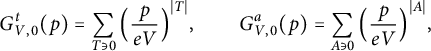(1.1) $$ \begin{align} G_{V,0}^t(p) = \sum_{T \ni 0} \Big(\frac{p}{eV} \Big)^{{\lvert T \rvert}} , \qquad G_{V,0}^a(p) = \sum_{A \ni 0} \Big(\frac{p}{eV} \Big)^{{\lvert A \rvert}} , \end{align} $$

where the first sum is over all labeled trees T in $\mathbb {K}_V$ containing the vertex $0$ , the second sum is over all labeled connected subgraphs A containing $0$ , and $|T|$ and $|A|$ denote the number of edges in T and A. The division of p by $eV$ is a normalisation to make $p=1$ correspond to a critical value. We also study the two-point functions

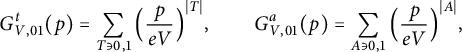(1.2) $$ \begin{align} G_{V,01}^t(p) = \sum_{T \ni 0,1} \Big(\frac{p}{eV} \Big)^{{\lvert T \rvert}} , \qquad G_{V,01}^a(p) = \sum_{A \ni 0,1} \Big(\frac{p}{eV} \Big)^{{\lvert A \rvert}} , \end{align} $$

where the sums now run over trees or connected subgraphs containing the distinct vertices $0,1$ . To avoid repetition, when a formula applies to both trees and connected subgraphs we often omit the superscripts $t,a$ . With this convention, we define the susceptibility

(1.3) $$ \begin{align} \chi_V(p) = G_{V,0}(p)+(V-1)G_{V,01}(p). \end{align} $$

We are particularly interested in values of p in a critical window $p=1+sV^{-1/2}$ around the critical point, with $s \in \mathbb {R}$ .

We define the profile

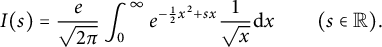(1.4) $$ \begin{align} I(s) = \frac{e}{\sqrt{2\pi}}\int_0^\infty e^{-\frac 12 x^2+sx}\frac{1}{\sqrt{x}} \mathrm d x \qquad (s \in \mathbb{R}). \end{align} $$

The profile can be rewritten in terms of a Faxén integral [25, p. 332] as $I (s) = e\pi ^{-1/2}2^{-5/4} \mathrm {Fi} ( \frac {1}{2}, \frac {1}{4}; \sqrt {2} s )$ , and its asymptotic behavior is given by [25, Example 7.3, p. 84] to be

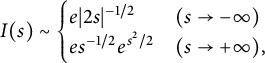(1.5) $$ \begin{align} I (s) \sim \begin{cases} e |2s|^{-1/2} & (s \to -\infty) \\ e s^{-1/2}e^{s^2/2} & (s \to +\infty) , \end{cases} \end{align} $$

where $f \sim g$ means $\lim f/g = 1$ . Our main result is the following theorem.

Theorem 1.1 For both trees and connected subgraphs, and for all $s \in \mathbb {R}$ , as $V \to \infty $ we have

(1.6) $$ \begin{align} G_{V,01}(1 + sV^{-1/2}) & \sim V^{-3/4} I(s) , \end{align} $$

(1.7) $$ \begin{align} \chi_V(1 + sV^{-1/2}) &\sim V^{1/4} I(s). \end{align} $$

The proof of Theorem 1.1 uses a uniform bound on the one-point function. The following theorem gives a statement that is more precise than a bound. It involves the principal branch $W_0$ of the Lambert function [5], which solves $W_0e^{W_0} =z$ and has power series

(1.8) $$ \begin{align} W_0(z) = \sum_{n=1}^\infty \frac{(-n)^{n-1}}{n!}z^n. \end{align} $$

The solution to $W_0e^{W_0} = -1/e$ is achieved by the particular value $W_0(-1/e)=-1$ .

Theorem 1.2 For both trees and connected subgraphs, for all $s \ge 0$ , and for all sequences $p_V$ with $p_V \le 1+sV^{-1/2}$ and $\lim _{V\to \infty }p_V=p\in [0,1]$ ,

(1.9) $$ \begin{align} \lim_{V\to\infty} G_{V,0}(p_V) &= \sum_{n=1}^\infty \frac{ n^{n-1} }{n!} \Big( \frac{p}{e} \Big)^{n-1} = -\frac{e}{p}W_0\Big(\!\!-\frac{p}{e} \Big). \end{align} $$

In particular, if $p=1$ then $\lim _{V\to \infty } G_{V,0}(p_V) = e$ .

Notation: We write $f \lesssim g$ if there is a $C>0$ such that $f(x) \le C g(x)$ for all x of interest.

1.2 Method of proof

To prove (1.6), it suffices to prove (1.7) and (1.9), since when $p=1+sV^{-1/2}$ , by definition of $\chi _V$ we then have

(1.10) $$ \begin{align} G_{V,01} = \frac{ \chi_V - G_{V,0} } {V - 1 } \sim \frac {\chi_V} V. \end{align} $$

1.2.1 Trees

By Cayley’s formula, the number of trees on n labeled vertices is $n^{n-2}$ . By decomposing the sum defining $G_{V,0}^t(p)$ according to the number n of vertices in the tree, and by counting the number of ways to choose $n-1$ vertices other than $0$ , we have

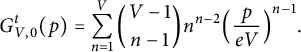(1.11) $$ \begin{align} G_{V,0}^t(p) &= \sum_{n=1}^{V} \binom{V-1}{n-1} n^{n-2} \Big(\frac{p}{eV} \Big)^{n-1}. \end{align} $$

Similarly, by counting the number of ways to choose $n-2$ vertices other than $0$ and  $1$ , we have

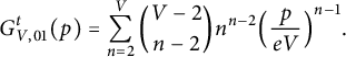(1.12) $$ \begin{align} G_{V,01}^t(p) = \sum_{n=2}^{V} \binom{V-2}{n-2} n^{n-2} \Big(\frac{p}{eV} \Big)^{n-1}. \end{align} $$

Since

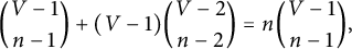(1.13) $$ \begin{align} \binom{V-1}{n-1} + (V-1) \binom{V-2}{n-2} = n\binom{V-1}{n-1}, \end{align} $$

it follows from (1.3) that the susceptibility is given by

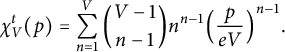(1.14) $$ \begin{align} \chi_{V}^t(p) &= \sum_{n=1}^{V} \binom{V-1}{n-1} n^{n-1} \Big(\frac{p}{eV} \Big)^{n-1}. \end{align} $$

For trees, we prove Theorems 1.1 and 1.2 by directly analyzing the above series for $\chi _V^t$ and $G_{V,0}^t$ . The profile $I(s)$ for $\chi _V^t(1 + sV^{-1/2})$ arises from a Riemann sum limit.

1.2.2 Connected subgraphs

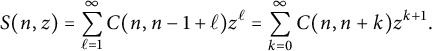
For connected subgraphs, we will show that the contribution to $\chi _V^a, G_{V,01}^a$ from connected subgraphs with cycles is much smaller than the contribution from trees. Let $C(n,n-1+\ell )$ denote the number of connected graphs on n labeled vertices with exactly $n-1+\ell $ edges, i.e., with $\ell $ surplus edges. The surplus must be zero for $n=1,2$ . For $n\ge 3$ , we define the surplus generating function

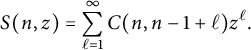(1.15) $$ \begin{align} S(n,z) = \sum_{\ell= 1}^\infty C(n,n-1+\ell) z^{\ell}. \end{align} $$

Note that terms in the above sum are zero unless $\ell \le \binom {n} 2 - (n-1)$ , and that the tree term ( $\ell =0$ ) is absent.

We decompose the sums defining $G_{V,0}^a$ and $G_{V,01}^a$ according to the number n of vertices in the connected subgraph, and we further distinguish whether or not the subgraph contains surplus edges. This leads to the decomposition

(1.16) $$ \begin{align} G_{V,0}^a(p) &= G_{V,0}^t(p) + \Delta_{V,0}(p), \end{align} $$

(1.17) $$ \begin{align} \chi_{V}^a(p) &= \chi_{V}^t(p) + \Delta_{V}(p), \end{align} $$

with

(1.18) $$ \begin{align} \Delta_{V,0}(p) &= \sum_{n=3}^{V} \binom{V-1}{n-1} S\Big(n,\frac p {eV}\Big) \Big(\frac{p}{eV} \Big)^{n-1} , \end{align} $$

(1.19) $$ \begin{align} \Delta_{V}(p) & = \sum_{n=3}^{V} \binom{V-1}{n-1} n S\Big(n,\frac p {eV}\Big) \Big(\frac{p}{eV} \Big)^{n-1}. \end{align} $$

Given Theorems 1.1 and 1.2 for trees, we prove Theorems 1.1 and 1.2 for connected subgraphs by showing that, for all $s\in \mathbb {R}$ ,

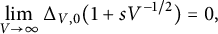(1.20) $$ \begin{align} \lim_{V\to\infty} \Delta_{V,0}(1+sV^{-1/2}) & =0, \end{align} $$

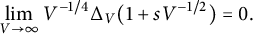(1.21) $$ \begin{align} \lim_{V\to\infty} V^{-1/4}\Delta_V(1 + sV^{-1/2}) &= 0. \end{align} $$

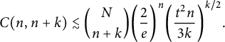
The proof is more subtle than for trees and requires estimates on the surplus generating function. As we discuss later, a precise but cumbrous asymptotic formula for $C(n,n+k)$ is given in [3, Corollary 1]. We use that formula to prove the following useful explicit bound. By convention, $k^k = 1$ when $k=0$ .

Proposition 1.3 Let $n \ge 3$ and $N = \binom n 2$ . For $0 \le k \le n$ , we have

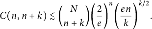(1.22) $$ \begin{align} C(n, n+k) \lesssim \binom N {n+k} \bigg( \frac 2 e \bigg)^n \bigg( \frac{ e n }{ k }\bigg)^{k/2}. \end{align} $$

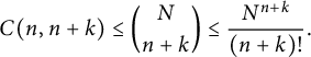
Proposition 1.3 is most useful when the surplus $\ell = k+1$ is small but of order n. This is a delicate region when controlling the surplus generating function, and the precise constant e in the last factor of (1.22) is important. For a larger surplus, we simply bound $C(n,n+k)$ by the total number of graphs (connected or not) on n vertices with $n+k$ edges, which is $\binom {N}{n+k}$ . Together, these bounds provide enough control on $S(n,p/(eV))$ to prove (1.20) and (1.21).

1.3 Motivation

Theorem 1.1 is motivated by a broader emerging theory of finite-size scaling in statistical mechanical models above their upper critical dimensions. The theory involves a family of profiles expressed in terms of the functions

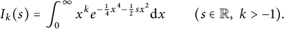(1.23) $$ \begin{align} I_k(s) = \int_0^\infty x^{k} e^{-\frac 14 x^4 - \frac 12 s x^2} \mathrm dx \qquad (s\in \mathbb{R}, \; k>-1). \end{align} $$

A change of variables transforms the profile I of (1.4) into $I(s)= e 2^{1/4}\pi ^{-1/2} I_0(-\sqrt {2}s)$ . The general theory is described in [21] with references to the extensive physics and mathematics literature.

Given an integer $d \ge 2$ , infinite-volume models can be formulated on a transitive graph $\mathbb {G}=(\mathbb {Z}^d,\mathbb {E})$ , whose edge set $\mathbb {E}$ has a finite number of edges containing the origin and is invariant under the symmetries of $\mathbb {Z}^d$ . Above an upper critical dimension $d_{\mathrm {c}}$ , for many models it has been proven that the critical exponents that describe the critical behavior are the same as the corresponding exponents when the model is formulated on a regular tree or on the complete graph. The tree and complete graph settings are easy to analyze. Finite-volume models (with periodic boundary conditions) can instead be formulated on a discrete torus $\mathbb {G}_r = (\mathbb {T}_r^d,\mathbb {E}_r)$ of period r. At and above the upper critical dimension, the torus models are known or conjectured to have critical behavior analogous to that seen on the complete graph, with an interesting “plateau” phenomenon involving a universal profile which is often expressed in terms of $I_k$ . The value of k depends on the model. Dimensions $d<d_{\mathrm {c}}$ are conjectured to exhibit different scaling, with no plateau or profile.

Lattice trees and lattice animals: A lattice animal is a finite connected subgraph of $\mathbb {G}$ , and a lattice tree is an acyclic lattice animal. The critical behavior of lattice trees and lattice animals is at least as difficult as is the case for the notoriously difficult self-avoiding walk. Despite significant interest from chemists and physicists for over half a century, due to applications to branched polymers [15], the critical behavior is understood mathematically only in dimensions $d>d_{\mathrm {c}} = 8$ . For $d>8$ , it has been proved using the lace expansion that for sufficiently large edge sets $\mathbb {E}$ (or for nearest-neighbor edges with d sufficiently large), lattice trees and lattice animals at the critical point both have the same behavior as a critical branching process [4, 6, 12, 13].

For $x\in \mathbb {Z}^d$ , let $c_m(x)$ denote the number of lattice trees or lattice animals containing $0,x$ and having exactly m bonds. The one-point functions, two-point functions, and susceptibilities are defined by

(1.24) $$ \begin{align} g(z) = \sum_{m=0}^\infty c_m(0)z^m, \quad G_z(x) = \sum_{m=0}^\infty c_m(x)z^m, \quad \chi(z) = \sum_{x\in \mathbb{Z}^d} G_z(x). \end{align} $$

The radius of convergence $z_{\mathrm {c}}$ (the critical point) of these series is finite and positive, and is strictly smaller for animals than for trees [7]. High-dimensional versions and extensions of Theorem 1.2 for $g(z_c)$ are proved in [19, 23]. The analogous quantities for trees and animals on the torus $\mathbb {T}_r^d$ are denoted $g_r(z)$ , $G_{r,z}(x)$ , $\chi _r(z)$ . These are polynomials in z, so they define entire functions of z. Nevertheless, for large r the infinite-volume critical point $z_c$ plays a role in the scaling. We denote the volume of the torus by $V=r^d$ .

Our computation of the profile I for the two-point function and susceptibility in Theorem 1.1 supports the following conjecture from [22] that the profile $I_0$ (just a rescaled I) occurs for both lattice trees and lattice animals on the torus, above the upper critical dimension.

Conjecture 1.4 For lattice trees and lattice animals on $\mathbb {T}_r^d$ with $d>8$ , there are constants $a_d<0$ and $b_d>0$ (different constants for trees and animals) such that, as $V=r^d \to \infty $ ,

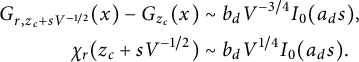(1.25) $$ \begin{align}\begin{aligned} G_{r,z_c+sV^{-1/2}}(x) -G_{z_c}(x) &\sim b_d V^{-3/4} I_0(a_d s), \\ \chi_r(z_c+sV^{-1/2}) &\sim b_d V^{1/4} I_0(a_d s). \end{aligned}\end{align} $$

In (1.25), the torus point x is identified with its representative in $\mathbb {Z}^d \cap (-\frac r2,\frac r2]^d$ in the evaluation of $G_{z_c}(x)$ . For $d>8$ , $G_{z_c}(x)$ decays as $|x|^{-(d-2)}$ [10, 11], and the constant term of order $V^{-3/4}= r^{-3d/4}$ dominates the Gaussian decay over most of the torus. This is the “plateau” phenomenon. On the complete graph, the decaying term ${\lvert x\rvert }^{-(d-2)}$ is absent, and only the constant term occurs for $G_{V,01}$ , as in (1.6). For ${d=d_{\mathrm {c}}=8}$ , the conjecture is modified to include logarithmic corrections to the window scale $V^{-1/2}$ , the plateau scale $V^{-3/4}$ , and the susceptibility scale $V^{1/4}$ , but with the identical profile $I_0$ .

Self-avoiding walk: Self-avoiding walk on the complete graph $\mathbb {K}_V$ is exactly solvable [27]. For $1 \le n \le V-1$ , let $c_{V,n}(0,1) = \prod _{j=2}^n (V-j)$ denote the number of n-step self-avoiding walks from $0$ to $1$ on $\mathbb {K}_V$ . Let $S_{V,01}(p) = \sum _{n=1}^{V-1} c_{V,n}(0,1)(p/V)^n$ and let $\chi _V^{\mathrm {SAW}}(p) = 1+(V-1)S_{V,01}(p)$ . It is proved in [27] (see also [24, Appendix B]) that, as $V \to \infty $ ,

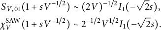(1.26) $$ \begin{align}\begin{aligned} S_{V,01}(1 + sV^{-1/2}) & \sim (2V)^{-1/2} I_1(-\sqrt{2} s) , \\ \chi_V^{\mathrm{SAW}}(1 + sV^{-1/2}) &\sim 2^{-1/2}V^{1/2} I_1(-\sqrt{2}s). \end{aligned}\end{align} $$

In [24, 26], the same profile $I_1$ is conjectured to apply to the self-avoiding walk on $\mathbb {T}_r^d$ for $d \ge 4$ , in the sense that the two-point function and susceptibility obey the analog of (1.25) with the right-hand sides replaced respectively by $b_d V^{-1/2} I_1(a_d s)$ and $ b_d V^{1/2} I_1(a_d s)$ . The conjectured log corrections for $d=4$ are indicated in [24, Section 1.6.3].

Spin systems: The plateau for spin systems in dimensions $d \ge d_{\mathrm {c}}=4$ is discussed in [20, 21, 26], including rigorous results for a hierarchical $|\varphi |^4$ model and conjectures for spin systems on the torus. The relevant profile for n-component spin systems is

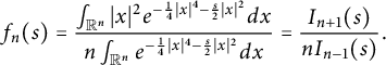(1.27) $$ \begin{align} f_n(s) = \frac{\int_{\mathbb{R}^n} |x|^2 e^{-\frac 14 |x|^4 - \frac s2 |x|^2} dx} {n\int_{\mathbb{R}^n} e^{-\frac 14 |x|^4 - \frac s2 |x|^2} dx} = \frac{ I_{n+1} (s)}{n I_{n-1} (s)}. \end{align} $$

The profile $f_1$ has been proven to occur for the Ising model on the complete graph (Curie–Weiss model); a recent reference is [2]. As $n \to 0$ , the profile $f_n(s)$ converges to $I_1(s)$ , which is consistent with the conventional wisdom that the spin model with $n=0$ corresponds to the self-avoiding walk.

Percolation: Percolation has been extensively studied both on infinite lattices [9] and on the complete graph (the Erdős–Rényi random graph) [17]. This is a probabilistic model in which the cluster containing $0$ is a connected subgraph $A \ni 0$ with weight $p^{{\lvert A \rvert }} (1-p)^{{\lvert {\partial A}\rvert }}$ , where ${\lvert A \rvert }$ denotes the number of edges in A, and $\partial A$ denotes the set of edges which are not in A but are incident to one or two vertices in A. On the complete graph, we divide p by V (not by $eV$ as in (1.2)) to make the critical value $p=1$ . Thus we define the two-point function

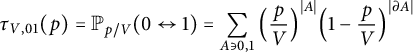(1.28) $$ \begin{align} \tau_{V,01}(p) = \mathbb{P}_{p/V}(0 \leftrightarrow 1) = \sum_{A \ni 0,1} \Big(\frac{p}{V} \Big)^{{\lvert A \rvert}} \Big(1-\frac{p}{V} \Big)^{{\lvert{\partial A} \rvert}} \end{align} $$

and the susceptibility (expected cluster size) $\chi _V ^{\mathrm {{perc}}}(p) = 1 +(V-1)\tau _{V,01}(p)$ . Our conjecture for an analog of Theorem 1.1 for percolation on the complete graph is as follows. It involves the Brownian excursion $W^*$ of length $1$ , and the moment generating function $\Psi (x) = \mathbb {E} \exp [ x\int _0^1 W^*(t)\mathrm dt] $ for the Brownian excursion area.

Conjecture 1.5 For $s\in \mathbb {R}$ , let

(1.29) $$ \begin{align} f_{\mathrm{perc}}(s) = \int_0^\infty x^2 \mathrm d\sigma_s, \qquad \mathrm d \sigma_s = \frac 1 { \sqrt{2\pi} } x^{-5/2} \Psi(x^{3/2}) e^{-\frac 1 6 x^3 + \frac s 2 x^2 - \frac{ s^2} 2 x} \mathrm dx. \end{align} $$

Then, for some $a,b>0$ , as $V\to \infty $ we have

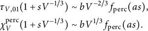(1.30) $$ \begin{align} \begin{aligned} \tau_{V,01}(1+sV^{-1/3}) & \sim b V^{-2/3} f_{\mathrm{perc}}(as), \\ \chi_{V} ^{\mathrm{{perc}}}(1+sV^{-1/3}) & \sim b V^{1/3} f_{\mathrm{perc}}(as). \end{aligned} \end{align} $$

Note the different powers of V in (1.30) compared to (1.25) and (1.6)–(1.7). The powers of V in (1.30) are well-known, but to our knowledge the occurrence of the profile has not been proved. On the torus $\mathbb {T}_r^d$ with $d>6$ , the powers $V^{-1/3}, V^{-2/3}, V^{1/3}$ are proved in [14], and the role of $f_{\mathrm {perc}}$ was first conjectured in [20, Appendix C].

The origin of the conjecture is as follows. The properly rescaled cluster size (without expectation) is known to converge in distribution to a random variable described by the Brownian excursion [1], and the limiting random variable is characterized by a point process [18]. The measure $\sigma _s$ is the intensity of the point process and is found in [18, Theorem 4.1]. The point process describes cluster sizes, in the sense that

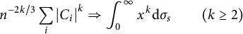(1.31) $$ \begin{align} n^{-2k/3} \sum_i {\lvert { C_i } \rvert}^k \Rightarrow \int_0^\infty x^k \mathrm d\sigma_s \qquad (k \ge 2) \end{align} $$

in distribution [1]. The $k=2$ case corresponds to $\chi _V^{\mathrm {{perc}}}$ and identifies $f_{\mathrm {perc}}(s)$ .

2 Proof for trees

We begin with an elementary lemma.

Lemma 2.1 Let $\gamma \ge 0$ , $\kappa> 0$ , and $\lambda \in \mathbb {R}$ . There is a constant $C_{\kappa , \lambda }>0$ such that

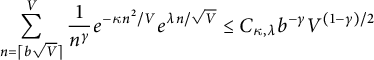(2.1) $$ \begin{align} \sum_{n=\lceil b \sqrt V \rceil}^{V} \frac{ 1 }{n^\gamma} e^{- \kappa n^2/V} e^{\lambda n/\sqrt{V}} \le C_{\kappa,\lambda} b^{-\gamma} V^{ (1 - \gamma) /2} \end{align} $$

for all V and for all b sufficiently large (depending on $\kappa ,\lambda $ ).

Proof Since $n \ge b\sqrt V$ and $\gamma \ge 0$ , the left-hand side of (2.1) is bounded by

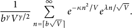(2.2) $$ \begin{align} \frac{1}{b^\gamma V^{\gamma / 2}} \sum_{n=\lceil b \sqrt V \rceil}^{\infty} e^{- \kappa n^2/V} e^{\lambda n/\sqrt{V}}. \end{align} $$

For b sufficiently large (depending on $\kappa ,\lambda $ ), the summand above is monotone decreasing in n, so we can bound the sum by the integral

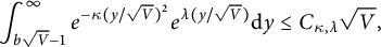(2.3) $$ \begin{align} \int_{b \sqrt V - 1}^\infty e^{- \kappa ( y / \sqrt V )^2} e^{\lambda( y/\sqrt{V}) } \mathrm dy \le C_{\kappa, \lambda} \sqrt V , \end{align} $$

and the desired result follows.

Proof of Theorem 1.1 for trees

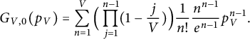
We use (1.14) and drop the superscript t. Fix $s\in \mathbb {R}$ . For $p = 1 + s V^{-1/2}$ , by combining $V^{-(n-1)}$ with the binomial coefficient, we have

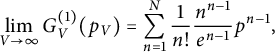
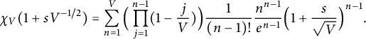(2.4) $$ \begin{align} \chi_V(1+sV^{-1/2}) = \sum_{n=1}^{V} \Big(\prod_{j=1}^{n-1}( 1 - \frac jV )\Big) \frac 1 {(n-1)!} \frac{n^{n-1}}{e^{n-1}} \Big(1+\frac s {\sqrt{V}} \Big)^{n-1}. \end{align} $$

Let $0 < a < 1 < b < \infty $ . We divide the sum over n into three parts $\chi _V ^{(1)}, \chi _V ^{(2)}, \chi _V ^{(3)}$ , which respectively sum over n in the intervals $[1, a \sqrt V)$ , $[ a \sqrt V, b \sqrt V]$ , $(b \sqrt V , V]$ . We will prove that

(2.5) $$ \begin{align} \chi_V ^{(1)} \lesssim e^{a{\lvert s\rvert}} ( 1 + a^{1/2} V^{1/4}), \qquad \chi_V ^{(3)} \le C_{{\lvert s\rvert}} b^{-1/2} V^{1/4} \end{align} $$

for all $a>0$ and all b sufficiently large, and that

(2.6) $$ \begin{align} \lim_{V\to \infty} V^{-1/4} \chi_V^{(2)} = \int_a^b f(x) \mathrm d x , \qquad f(x) = \frac{e}{\sqrt{2\pi}}e^{-x^2/2}\frac{1}{\sqrt{x}} e^{sx} \end{align} $$

for all $a,b$ . These claims imply that

(2.7) $$ \begin{align} \int_a^b f(x) \mathrm d x \le \liminf_{V\to \infty} \frac{ \chi_V }{V^{1/4}} \le \limsup_{V\to \infty} \frac{ \chi_V }{V^{1/4}} \le C e^{a{\lvert s\rvert}}a^{1/2}+ \int_a^b f(x) \mathrm d x + C_{|s|} b^{-1/2} \end{align} $$

for all $a> 0$ and all b sufficiently large. Since $\chi _V$ does not depend on a or b, by taking the limits $a\to 0$ , $b\to \infty $ , we obtain $\lim _{V\to \infty } V^{-1/4} \chi _V = \int _0^\infty f$ , which is the desired result (1.7).

It remains to prove the claims (2.5) and (2.6). Let

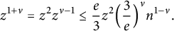
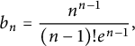(2.8) $$ \begin{align} b_{n} = \frac{n^{n-1}}{(n-1)!e^{n-1}} , \end{align} $$

which obeys $b_{n} \lesssim 1/\sqrt {n}$ , by Stirling’s formula. Using this in the sum for $\chi _V ^{(1)}$ , and using $1 + s/\sqrt V \le e^{ {\lvert s\rvert } / \sqrt V}$ , we get

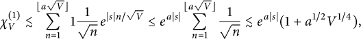(2.9) $$ \begin{align} \chi_V^{(1)} \lesssim \sum_{n=1}^{\lfloor a \sqrt V \rfloor} 1 \frac{1}{\sqrt {n} } e^{ |s| n / \sqrt V} \le e^{a{\lvert s\rvert}} \sum_{n=1}^{\lfloor a \sqrt V \rfloor} \frac{1}{\sqrt {n} } \lesssim e^{a{\lvert s\rvert}} ( 1 + a^{1/2} V^{1/4} ) , \end{align} $$

as claimed. For $\chi _V ^{(3)}$ , we also need a bound on the product over j. Using $1-x \le e^{-x}$ , we have

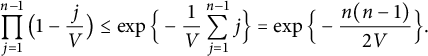(2.10) $$ \begin{align} \prod_{j=1}^{n-1}\big( 1 - \frac jV \big) \le \exp\Big\{ - \frac 1 V \sum_{j=1}^{n-1} j \Big\} = \exp \Big\{ - \frac { n (n-1)} {2V} \Big\}. \end{align} $$

By Lemma 2.1 with $\gamma = \kappa = \frac {1}{2}$ and $\lambda =|s|$ , this implies that, for all b sufficiently large,

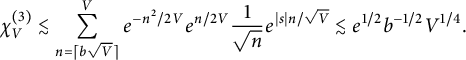(2.11) $$ \begin{align} \chi_V^{(3)} \lesssim \sum_{n= \lceil b \sqrt V \rceil}^{V} e^{-n^2/2V} e^{n/2V} \frac{1}{\sqrt{ n}} e^{|s|n/\sqrt{V}} \lesssim e^{1/2} b^{-1/2} V^{1/4}. \end{align} $$

Finally, for $\chi _V ^{(2)}$ we fix $a,b$ and use the asymptotic formulas

(2.12) $$ \begin{align} \Big( 1 + \frac s {\sqrt V} \Big)^{n-1} &= \exp \Big\{ (n-1) \log( 1 + \frac s {\sqrt V} ) \Big\} = e^{s n/ \sqrt V} \Big[ 1 + O\Big(\frac 1 { \sqrt V }\Big) + O\Big(\frac n V\Big) \Big] , \end{align} $$

(2.13) $$ \begin{align} \prod_{j=1}^{n-1}\big( 1 - \frac jV \big) &= \exp\Big\{\sum_{j=1}^{n-1} \log(1-\frac j V)\Big\} = e^{-n^2/2V} \Big[ 1 +O\Big(\frac n V\Big) + O\Big(\frac {n^3} {V^2}\Big)\Big] , \end{align} $$

which follow from Taylor expansion of the logarithm (the constants here depend on s). Since $n \in [a\sqrt V, b\sqrt V]$ , the above, together with the fact that $b_{n} = \frac { e }{\sqrt {2\pi n}}[1+O(1/n)]$ by Stirling’s formula, give

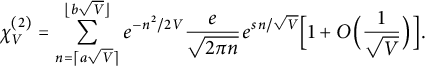(2.14) $$ \begin{align} \chi_V^{(2)} & = \sum_{n= \lceil a \sqrt V \rceil}^{ \lfloor b \sqrt V \rfloor} e^{-n^2 / 2V} \frac{e}{\sqrt{2\pi n}} e^{sn/\sqrt{V}} \Big[ 1 + O\Big(\frac 1 {\sqrt V}\Big) \Big]. \end{align} $$

The desired limit then follows from the observations that the leading term of $V^{-1/4} \chi _V ^{(2)}$ is a Riemann sum for the integral $\int _a^b f$ with mesh size $V^{-1/2}$ .

Proof of Theorem 1.2 for trees

We use (1.11) and again drop the superscript t. Fix $s\ge 0$ . Let $p_V$ be a sequence with $p_V \le 1 + s V^{-1/2}$ and $p_V \to p \in [0,1]$ . Similarly to (2.4) and with an additional factor of n in the denominator,

(2.15) $$ \begin{align} G_{V,0}(p_V) = \sum_{n=1}^{V} \Big(\prod_{j=1}^{n-1}( 1 - \frac jV )\Big) \frac 1 {n!} \frac{n^{n-1}}{e^{n-1}} p_V^{n-1}. \end{align} $$

Let $N, b\ge 1$ . We divide the sum over n into three parts $G_V ^{(1)}, G_V ^{(2)}, G_V ^{(3)}$ , which respectively sum over n in the intervals $[1, N]$ , $( N, b \sqrt V]$ , $(b \sqrt V , V]$ . For a fixed N, we immediately get

(2.16) $$ \begin{align} \lim_{V\to \infty} G^{(1)}_{V}(p_V) = \sum_{n=1}^N \frac{1}{n!} \frac{n^{n-1}}{e^{n-1}}p^{n-1}, \end{align} $$

which dominates the sum. Indeed, using monotonicity of the generating function, for $G_V ^{(2)}$ we can proceed as in (2.9) to bound

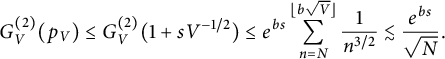(2.17) $$ \begin{align} G_V ^{(2)} (p_V) \le G_V ^{(2)} (1 + s V^{-1/2}) \le e^{bs} \sum_{n=N}^{ \lfloor b\sqrt V \rfloor} \frac 1 {n^{3/2}} \lesssim \frac{ e^{bs} } { \sqrt N}. \end{align} $$

For $G_V ^{(3)}$ , we can argue as in (2.11) but with an additional factor n in the denominator, and use Lemma 2.1 with $\gamma = \frac 3 2$ to get $G_V ^{(3)} (p_V) \lesssim b^{-3/2}V^{-1/4}$ for b sufficiently large. Together, we obtain

(2.18) $$ \begin{align} \sum_{n=1}^N \frac{1}{n!} \frac{n^{n-1}}{e^{n-1}}p^{n-1} \le \liminf_{V\to \infty} G_{V,0} \le \limsup_{V\to \infty} G_{V,0} \le \sum_{n=1}^N \frac{1}{n!} \frac{n^{n-1}}{e^{n-1}}p^{n-1} + \frac{ C e^{bs} } { \sqrt N} \end{align} $$

for all $N \ge 1$ and all b sufficiently large. Since $G_{V,0}$ does not depend on N, we can take the limit $N \to \infty $ to conclude the desired result (1.9).

3 Proof for connected subgraphs

3.1 Bound on $C(n,n+k)$

We use the asymptotic formula for $C(n,n+k)$ proved in [3]. We follow the notation in [3] and write

(3.1) $$ \begin{align} x = 1 + \frac k n. \end{align} $$

For $x> 1$ , we define the function $y = y(x) \in (0,1)$ implicitly by

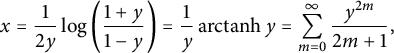(3.2) $$ \begin{align} x = \frac{1}{2y} \log \bigg( \frac { 1+ y } { 1 - y } \bigg) = \frac{1}{y}\operatorname{\mathrm{arctanh}} y = \sum_{m = 0}^\infty \frac{ y^{2m} } { 2m+1 } , \end{align} $$

and we define the functions $\varphi (x)$ , $a(x)$ by

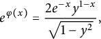(3.3) $$ \begin{align} e^{\varphi(x)} = \frac{ 2 e^{-x} y^{1-x} }{ \sqrt{ 1 - y^2} } , \end{align} $$

(3.4) $$ \begin{align} a(x) = x(x+1)(1-y) + \log( 1 - x + xy) - \frac{1}{2} \log( 1 - x + x y^2 ). \end{align} $$

Both $\varphi $ and a extend continuously to $x=1$ by defining $y^{1-x} = 1$ at $x=1$ and defining $a(1) = 2 + \frac {1}{2} \log \frac 3 2$ .

Let $N = \binom n 2$ . It is proved in [3, Corollary 1] that there are constants $w_k = 1 + O(1/k)$ for which

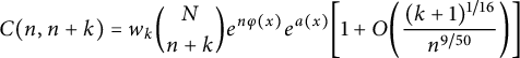(3.5) $$ \begin{align} C(n,n+k) = w_k \binom N {n+k} e^{n \varphi(x)} e^{a(x)} \bigg[ 1 + O\bigg( \frac { (k+1)^{1/16} }{ n^{9/50} } \bigg) \bigg] \end{align} $$

uniformly in $0 \le k \le N - n$ . The constants $w_k$ are related to Wright’s constants for the asymptotics of $C(n,n+k)$ with k fixed [29], and they are related to the Brownian excursion area [28]. We will simply bound $w_k$ by a constant. The next lemma gives estimates for $\varphi (x)$ and $a(x)$ .

Lemma 3.1 Let $x\ge 1$ .

1. (i) The function $a(x)$ is bounded.

2. (ii) Let $t = \sqrt {3e}$ and $y = y(x)$ . Then

   (3.6) $$ \begin{align} e^{\varphi(x) } \le \frac 2 e \exp\Big\{ - \frac 1 3 y^2 \log \frac y t \Big\} , \end{align} $$
   and the right-hand side is monotonically increasing for $0 < y \le t/\sqrt e$ .

By considering the limit $x\to \infty $ ( $y\to 1$ ), we expect that the inequality (3.6) becomes optimal with $t = (e/2)^3 \approx 2.51$ , but we do not pursue this. The weaker version with $t= \sqrt {3e}$ is sufficient for our purposes, but to show the role of t we keep it in our formulas.

Proof (i) The function $a(x)$ is continuous on $[1,\infty )$ by definition, and it satisfies ${\lvert a(x)\rvert } \lesssim x^2 (1-y) \sim 2x^2 e^{-2x}$ as $x\to \infty $ by [3, Lemma 3.2], so it is bounded.

(ii) By the definitions of $\varphi (x)$ and x, and by the Taylor series for $\log (1-y^2)$ ,

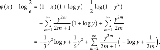(3.7) $$ \begin{align} \varphi(x) - \log \frac 2 e &= (1-x) ( 1 + \log y ) - \frac{1}{2} \log ( 1 - y^2 ) \nonumber \\ &= - \sum_{m=1}^\infty \frac{ y^{2m} } { 2m+1 } ( 1 + \log y ) + \sum_{m=1}^\infty \frac{ y^{2m} } { 2m } \nonumber \\ &= - \frac 1 3 y^2 \log y + \frac 1 6 y^2 + \sum_{m=2}^\infty \frac{ y^{2m} }{2m+1} \Big(-\log y + \frac 1 {2m} \Big). \end{align} $$

We bound the series in the last line by a quadratic function, term by term. For any $m\ge 2$ , by calculus,

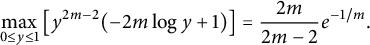(3.8) $$ \begin{align} \max_{0 \le y \le 1} \big[ y^{2m-2} (-2m \log y + 1) \big] = \frac{2m}{2m-2} e^{-1/m}. \end{align} $$

Then, with $K = \max _{m\ge 2} \{ \frac {2m}{2m-2} e^{-1/m} \} = 2 e^{-1/2}$ , by [8, 0.234.8] we have

(3.9) $$ \begin{align} \sum_{m=2}^\infty \frac{ y^{2m} }{2m+1} \Big(-\log y + \frac 1 {2m} \Big) \le \sum_{m=2}^\infty \frac{ K y^2 }{(2m+1)(2m)} = (1 - \log 2 - \frac 1 6) K y^2. \end{align} $$

Therefore,

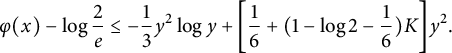(3.10) $$ \begin{align} \varphi(x) - \log \frac 2 e \le - \frac 1 3 y^2 \log y + \bigg[ \frac 1 6 + (1 - \log 2 - \frac 1 6)K \bigg] y^2. \end{align} $$

This implies (3.6) with any t that obeys $ \frac 1 3 \log t \ge \frac 1 6 + (1 - \log 2 - \frac 1 6)K \approx 0.3367$ . In particular, we can take any $t \ge 2.75$ , including $t = \sqrt {3e} \approx 2.85$ . Monotonicity of the upper bound in $0 < y \le t/\sqrt e$ is another calculus exercise.

We now restate and prove Proposition 1.3.

Proposition 3.2 Let $n \ge 3$ , $N = \binom n 2$ , and $t=\sqrt {3e}$ . For $0 \le \frac k n \le \frac {t^2}{3e}$ , we have

(3.11) $$ \begin{align} C(n, n+k) \lesssim \binom N {n+k} \bigg( \frac 2 e \bigg)^n \bigg( \frac{ t^2 n }{ 3 k }\bigg)^{k/2}. \end{align} $$

Proof We use the asymptotic formula (3.5), and use that $w_k = 1 + O(1/k)$ is bounded. The error term in (3.5) is bounded by a constant since k is at most linear in n. The factor $e^{a(x)}$ is also bounded by a constant, by Lemma 3.1(i). We therefore only need to estimate $e^{n\varphi (x)}$ . Since $0 \le \frac k n \le \frac {t^2}{3e}$ and $x = 1 + \frac k n$ , by (3.2) we have $y(x) \le \sqrt {3(x-1)} = \sqrt { 3k / n } \le t / \sqrt e$ , so Lemma 3.1(ii) gives

(3.12) $$ \begin{align} e^{\varphi(x)} \le \frac 2 e \exp\Big\{ - \frac 1 3 y^2 \log \frac y t \Big\} \le \frac 2 e \exp\Big\{ - \frac {x-1}2 \log \frac {3(x-1)} {t^2} \Big\} = \frac 2 e \bigg( \frac {t^2 n}{3k} \bigg)^{k/2n}. \end{align} $$

The desired result then follows by inserting the above into (3.5).

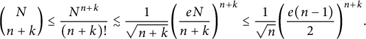
For larger $\frac kn$ we simply use the fact that $C(n,n+k)$ is less than the total number of graphs (connected or not) on n vertices with $n+k$ edges, which is $\binom {N}{n+k}$ . For all $n \ge 2$ and $k \ge -1$ , we have

(3.13) $$ \begin{align} C(n,n+k) \le \binom{N}{n+k} \le \frac{N^{n+k}}{(n+k)!}. \end{align} $$

3.2 Bound on the surplus generating function

We now prove useful bounds on the surplus generating function defined in (1.15):

(3.14) $$ \begin{align} S(n,z) & = \sum_{\ell= 1}^\infty C(n,n-1+\ell) z^{\ell} = \sum_{k=0}^\infty C(n,n+k) z^{k+1}. \end{align} $$

The terms in the series are zero unless $k \le \binom {n} 2 - n$ . The goal is to prove that $S(n,z)$ is small relative to the number of trees $C(n,n-1) = n^{n-2}$ . We do this by decomposing the series into two parts corresponding to sparse and dense graphs. We define

(3.15) $$ \begin{align} A(n,z) = \frac 1 { n^{n-2} } \sum_{k=0}^{n} C(n,n+k) z^{k+1} , \quad B(n,z) = \frac 1 { n^{n-2} } \sum_{k= \lfloor \frac 12 n \rfloor}^\infty C(n,n+k) z^{k+1} , \end{align} $$

so that

(3.16) $$ \begin{align} S(n,z) \le n^{n-2} \big( A(n,z) + B(n,z) \big). \end{align} $$

Lemma 3.3 (Sparse connected graphs)

Let $n \ge 3$ , $z \ge 0$ , and $t=\sqrt {3e}$ .

1. (i) If $n^{3/2} z \le b$ , then $A(n,z) \le C_b n^{3/2} z$ for some $C_b> 0$ .

2. (ii) If $\varepsilon> 0$ , then

   (3.17) $$ \begin{align} A(n,z) \le C_\varepsilon \exp\Big\{ \big(\frac{1}{24}+\varepsilon \big) e t^2 z^2 n^3 \Big\} \end{align} $$
   for some $C_\varepsilon> 0$ .

Proof Since $\frac {t^2}{3e} = 1$ , we can apply Proposition 3.2 to estimate $C(n,n+k)$ . For the binomial coefficient in (3.11), we use Stirling’s formula, $n+k \ge n$ , and $N = \binom n 2 = \frac {1}{2} n(n-1)$ to see that

(3.18) $$ \begin{align} \binom N {n+k} \le \frac{ N^{n+k} }{ (n+k)! } \lesssim \frac 1 { \sqrt{n+k} } \bigg( \frac {eN}{n+k} \bigg)^{n+k} \le \frac{1}{\sqrt{n}} \bigg( \frac {e (n-1) }{2} \bigg)^{n+k}. \end{align} $$

Then, by extending the sum to run over all $k \ge 0$ , we obtain

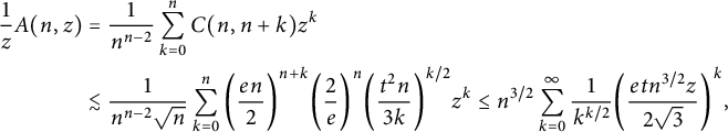(3.19) $$ \begin{align} \frac 1 z A(n,z) &= \frac 1 {n^{n-2}} \sum_{k=0}^{n} C(n,n+k) z^{k}\nonumber \\ &\lesssim \frac{1}{n^{n-2}\sqrt n} \sum_{k=0}^{n} \bigg( \frac {e n }{2} \bigg)^{n+k} \bigg( \frac 2 e \bigg)^n \bigg( \frac{ t^2 n }{ 3 k }\bigg)^{k/2} z^k \le n^{3/2} \sum_{k=0}^{\infty} \frac 1 {k^{k/2}} \bigg( \frac{etn^{3/2}z}{2\sqrt{3}} \bigg)^k , \end{align} $$

which converges for all $z>0$ .

(i) If $n^{3/2}z \le b$ then the series on the right-hand side is bounded by a constant $C_b$ , as required.

(ii) We set $x = \frac {etn^{3/2}z}{2\sqrt {3}}$ and use the asymptotic formula [16, Lemma 4.1(i)]

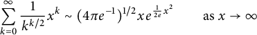(3.20) $$ \begin{align} \sum_{k=0}^{\infty} \frac{1}{k^{k/2}} x^k \sim (4\pi e^{-1})^{1/2} x e^{\frac{1}{2e}x^2} \qquad \text{as } x \to\infty \end{align} $$

to get a bound for large x. For smaller $x\ge 0$ , we simply bound by a constant. The desired result then follows by absorbing the prefactor of (3.20) and another factor of $n^{3/2}z = \mathrm {const}\,x$ into the exponential. This completes the proof.

Lemma 3.4 (Dense connected graphs)

Let $n\ge 3$ and $z\le \frac {3}{en}$ . Then $B(n,z)\lesssim z^2$ .

Proof Let $\nu = \lfloor n/2 \rfloor \ge 1$ . The crude bound (3.13) gives

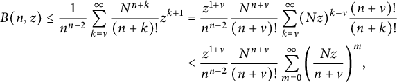(3.21) $$ \begin{align} B(n,z) \le \frac 1 {n^{n-2}} \sum_{k = \nu}^{\infty} \frac{N^{n+k}}{(n+k)!} z^{k+1} & = \frac {z^{1+\nu}} {n^{n-2}} \frac{N^{n+\nu}}{(n+\nu)!} \sum_{k = \nu}^{\infty} (Nz)^{k-\nu}\frac{(n+\nu)!}{(n+k)!} \nonumber\\ & \le \frac {z^{1+\nu}} {n^{n-2}} \frac{N^{n+\nu}}{(n+\nu)!} \sum_{m=0}^{\infty} \bigg( \frac{Nz}{n+\nu} \bigg)^{m} , \end{align} $$

since $(n+k)! \ge (n+\nu )! (n+ \nu )^{k - \nu }$ . Note that by our hypothesis

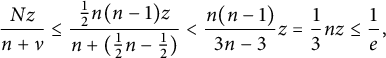(3.22) $$ \begin{align} \frac { Nz } { n+ \nu } \le \frac { \frac{1}{2} n (n-1) z } { n + (\frac{1}{2} n - \frac{1}{2})} < \frac { n (n-1)}{3n-3} z = \frac 1 3 {nz} \le \frac 1 e , \end{align} $$

so the geometric series in (3.21) is bounded by a constant. For the prefactor in (3.21), since $1+\nu \ge 2$ and $z\le \frac {3}{en}$ by hypothesis, we have

(3.23) $$ \begin{align} z^{1+\nu} = z^2 z^{ \nu - 1} \le \frac e 3 z^2 \Big( \frac{3}{e}\Big)^{\nu } n^{1 - \nu}. \end{align} $$

Also, using $N = \frac {1}{2} n(n-1)$ and Stirling’s formula,

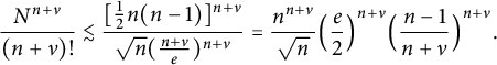(3.24) $$ \begin{align} \frac{ N^{n+\nu} }{(n+\nu)!} \lesssim \frac{ [\frac{1}{2} n (n-1) ]^{n+\nu} } { \sqrt n ( \frac{n+\nu}e )^{n+\nu} } = \frac {n^{n+\nu} } {\sqrt n } \Big( \frac{e}{2}\Big)^{n+\nu} \Big( \frac{n-1}{n+\nu} \Big)^{n+\nu}. \end{align} $$

Since $\frac {n-1}{n+\nu } \le \frac 2 3$ , together we obtain

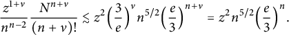(3.25) $$ \begin{align} \frac {z^{1+\nu}} {n^{n-2}} \frac{N^{n+\nu}}{(n+\nu)!} \lesssim z^2 \Big( \frac{3}{e}\Big)^{\nu } n^{5/2} \Big( \frac{e}{3}\Big)^{n+\nu} = z^2 n^{5/2} \Big( \frac{e}{3}\Big)^{n}. \end{align} $$

It follows that $B(n,z) \lesssim z^2 \sup _{n \ge 3} \{ n^{5/2} (e/3)^n \} , $ and the proof is complete since $e < 3$ .

3.3 Proof for connected subgraphs

Proof of Theorem 1.1 for connected subgraphs

Fix $s\in \mathbb {R}$ and let $p = 1 + sV^{-1/2}$ . We assume V is large enough so that $p \le 3$ . As discussed around (1.21), it suffices to prove

(3.26) $$ \begin{align} \lim_{V\to\infty} V^{-1/4}\Delta_V(1 + sV^{-1/2}) &= 0. \end{align} $$

By the definition of $\Delta _V$ in (1.19) and by (3.16),

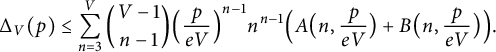(3.27) $$ \begin{align} \Delta_{V}(p) &\le \sum_{n=3}^{V} \binom{V-1}{n-1} \Big( \frac{p}{eV} \Big)^{n-1}n^{n-1} \Big( A \big(n, \frac{p}{eV} \big) + B\big(n, \frac{p}{eV}\big) \Big). \end{align} $$

We write the part of the upper bound (3.27) that contains $A,B$ as $\Delta _V ^{(A)}, \Delta _V ^{(B)}$ respectively.

We start with $\Delta _V ^{(B)}$ and use Lemma 3.4 to bound B. Let $z = p/(eV)$ . Since $n \le V$ and $p \le 3$ (for large V), we have $nz \le p / e \le 3/e$ , so Lemma 3.4 applies and gives $B(n,z) \lesssim V^{-2}$ . Then, by comparing to $\chi _V^t$ in (1.14), we find that

(3.28) $$ \begin{align} \Delta_V ^{(B)}(p) \lesssim V^{-2} \chi_V^t(p). \end{align} $$

For $\Delta _V ^{(A)}$ , we claim that if both $b \ge 1$ and V are sufficiently large, then

(3.29) $$ \begin{align} \Delta_V ^{(A)}(p) \le C_{b} V^{-1/4} \chi_V^t(p) + C_s b^{-1/2} V^{1/4}. \end{align} $$

Since we already know that $V^{-1/4} \chi _V^t$ converges, (3.29) implies that

(3.30) $$ \begin{align} 0 \le \limsup_{V\to \infty} \frac{ \Delta_V}{V^{1/4}} \le \limsup_{V\to \infty} \frac{ \Delta_V ^{(A)} + \Delta_V ^{(B)} }{V^{1/4}} \le C_{s} b^{-1/2} \end{align} $$

for all b sufficiently large. But $\Delta _V$ does not depend on b, so by taking the limit $b\to \infty $ , we obtain (3.26), as desired.

It remains to prove (3.29). We divide the sum defining $\Delta _V^{(A)}$ into two parts $\Delta _V ^{(1)}, \Delta _V ^{(2)}$ , which sum over n in the intervals $[3, b \sqrt V ]$ , $(b \sqrt V , V]$ respectively.

For $\Delta _V ^{(1)}$ , we have $n \le bV^{1/2}$ so $n^{3/2} z = n^{3/2}p/(eV) \le c_{b} V^{-1/4}$ , so we can apply Lemma 3.3(i) to obtain $A(n,z) \le C_b' n^{3/2} z \le C_b V^{-1/4}$ . With the formula for $\chi ^t_V$ in (1.14), this gives

(3.31) $$ \begin{align} \Delta_V ^{(1)} \le C_b V^{-1/4}\sum_{n=3}^{\lfloor b\sqrt V \rfloor} \binom{V-1}{n-1} \Big( \frac{p}{eV} \Big)^{n-1}n^{n-1} \le C_b V^{-1/4}\chi_V^t(p). \end{align} $$

This provides the first term on the right-hand side of (3.29).

For $\Delta _V ^{(2)}$ , we use $z=p/(eV)$ and Lemma 3.3(ii) to see that

(3.32) $$ \begin{align} A(n,z) \le C_\varepsilon \exp\Big\{ \big(\frac{1}{24}+\varepsilon \big) e^{-1} t^2 p^2 n^{3} / V^2 \Big\}. \end{align} $$

Since $t = \sqrt {3e}$ , we have $\frac 1 {24} e^{-1} t^2 = \frac 1 8$ . By choosing $\varepsilon $ small, and by using $p = 1 + s V^{-1/2} \to 1$ as $V\to \infty $ , for V sufficiently large (depending only on $\varepsilon ,s$ ) we have

(3.33) $$ \begin{align} A(n,z) \le C_\varepsilon \exp \Big\{ \frac 1 5 \frac { n^3 }{V^2 } \Big\}. \end{align} $$

For these values of V, we thus have

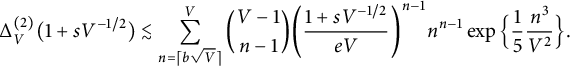(3.34) $$ \begin{align} \Delta_V ^{(2)}(1 + s V^{-1/2}) \lesssim \sum_{n=\lceil b\sqrt V \rceil}^{V} \binom{V-1}{n-1} \bigg( \frac{1 + s V^{-1/2}}{eV} \bigg)^{n-1} n^{n-1} \exp \Big\{ \frac 1 5 \frac { n^3 }{V^2 } \Big\}. \end{align} $$

We now follow the argument used for $\chi _V^{(3)}$ of trees in the paragraph containing (2.11). Using $\frac { n^3 }{V^2 } \le \frac { n^2 }{V }$ and Lemma 2.1 with $\gamma = \frac {1}{2}$ and $\kappa = \frac {1}{2} - \frac 15> 0$ , we find that if b is sufficiently large then

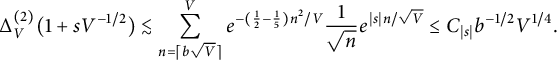(3.35) $$ \begin{align} \Delta_V ^{(2)}(1 + s V^{-1/2}) \lesssim \sum_{n=\lceil b \sqrt V \rceil}^{V} e^{- (\frac 1 2 - \frac 1 5) n^2 / V} \frac{1}{\sqrt{ n}} e^{|s|n/\sqrt{V}} \le C_{{\lvert s\rvert}} b^{-1/2} V^{1/4}. \end{align} $$

This gives the second term on the right-hand side of (3.29) and concludes the proof.

Proof of Theorem 1.2 for connected subgraphs

As noted at (1.20), it suffices to prove that $\Delta _{V,0}(1+sV^{-1/2}) \to 0$ for all $s \ge 0$ . We write $p = 1 + sV^{-1/2}$ and follow the proof of Theorem 1.1. Compared to $\Delta _V$ for the susceptibility, there is one less factor n in $\Delta _{V,0}$ , so instead of (3.27) we now have

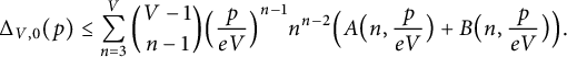(3.36) $$ \begin{align} \Delta_{V,0}(p) \le \sum_{n=3}^{V} \binom{V-1}{n-1} \Big( \frac{p}{eV} \Big)^{n-1}n^{n-2} \Big( A \big(n, \frac{p}{eV} \big) + B\big(n, \frac{p}{eV}\big) \Big). \end{align} $$

As in (3.28), the contribution from B obeys

(3.37) $$ \begin{align} \Delta_{V,0}^{(B)}(p) \lesssim V^{-2}G_{V,0}^t(p) \lesssim V^{-2}, \end{align} $$

so it vanishes in the limit. For $\Delta _{V,0}^{(1)}(p)$ , the same bound on A that was used in (3.31) now gives $\Delta _{V,0}^{(1)}(p) \le C_b V^{-1/4} G_{V,0}(p)$ . For $\Delta _{V,0}^{(2)}(p)$ , in (3.35) we now have an extra factor n in the denominator, so Lemma 2.1 with $\gamma = \frac 3 2$ gives

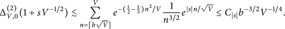(3.38) $$ \begin{align} \Delta_{V,0} ^{(2)}(1 + s V^{-1/2}) \lesssim \sum_{n= \lceil b \sqrt V \rceil}^{V} e^{- (\frac 1 2 - \frac 1 5) n^2 / V} \frac{1}{n^{3/2}} e^{|s|n/\sqrt{V}} \le C_{{\lvert s \rvert}} b^{-3/2} V^{-1/4}. \end{align} $$

Altogether, we have $\Delta _{V,0}(p) \lesssim V^{-1/4} \to 0$ , and the proof is complete.